
Database and Math Relations
31
For more Https://www.ThesisScientist.com Unit 4 Database and Math Relations Database and Math Relations A math relation is a Cartesian product of two sets. So if we change the order of theses two sets then the outcome of both will not be same. Therefore, the math relation changes by changing the order of columns. For Example , if there is a set A and a set B if we take Cartesian product of A and B then we take Cartesian product of B and A they will not be equal , so A x B = B x A Rests of the properties between them are same. Degree of a Relation We will now discuss the degree of a relation not to be confused with the degree of a relationship. You would be definitely remembering that the relationship is a link or association between one or more entity types and we discussed it in E-R data model. However the degree of a relation is the number of columns in that relation. For Example consider the table given below : STUDENT StID stName clName Sex S001 ajay MCS M S002 narendra BCS M S003 mohan MCS F S004 ritu MBA F S005 naveen BBA M Table 1: The STUDENT table Now in this example the relation STUDENT has four columns, so this relation has degree four. Cardinality of a Relation
-
Upload
prof-ansari -
Category
Engineering
-
view
136 -
download
0
Transcript of Database and Math Relations
For more Https://www.ThesisScientist.com
Unit 4
Database and Math Relations
Database and Math Relations
A math relation is a Cartesian product of two sets. So if we change the order of theses two sets then
the outcome of both will not be same. Therefore, the math relation changes by changing the order of
columns. For Example , if there is a set A and a set B if we take Cartesian product of A and B then
we take Cartesian product of B and A they will not be equal , so
A x B = B x A
Rests of the properties between them are same.
Degree of a Relation
We will now discuss the degree of a relation not to be confused with the degree of a relationship.
You would be definitely remembering that the relationship is a link or association between one or
more entity types and we discussed it in E-R data model.
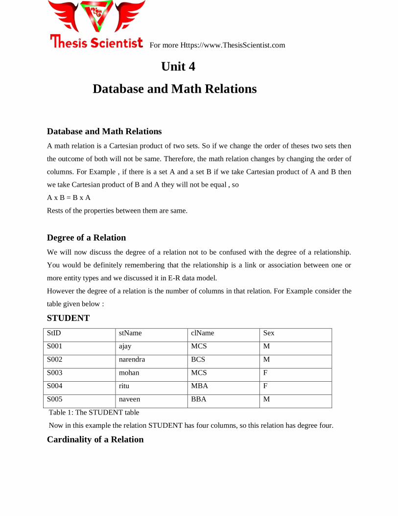
However the degree of a relation is the number of columns in that relation. For Example consider the
table given below :
STUDENT
StID stName clName Sex
S001 ajay MCS M
S002 narendra BCS M
S003 mohan MCS F
S004 ritu MBA F
S005 naveen BBA M
Table 1: The STUDENT table
Now in this example the relation STUDENT has four columns, so this relation has degree four.
Cardinality of a Relation

For more Https://www.ThesisScientist.com
The number of rows present in a relation is called as cardinality of that relation. For example, in
STUDENT table above, the number of rows is five, so the cardinality of the relation is five.
Foreign Key
An attribute of a table B that is primary key in another table A is called as foreign key. For Example,
consider the following two tables EM and DET :
EMP (ipDwd, empName, qual, depId)
DET cdiDwd, depName, numEmp)
In this example there are two relations; EM is having record of employees, whereas DET is having
record of different departments of an organization. Now in EM the primary key is empId, whereas in
DET the primary key is depId. The depId which is primary key of DET is also present in EMP so this
is a foreign key.
Requirements/Constraints of Foreign Key
Following are some requirements / constraints of foreign key :
There can be more than zero, one or multiple foreign keys in a table, depending on how many tables
a particular table is related with. For example in the above example the EMP table is related with the
DET table, so there is one foreign key depId, whereas DET table does not contain any foreign key.
Similarly, the EM table may also be linked with DESIG table storing designations, in that case EM
will have another foreign key and alike.
The foreign key attribute, which is present as a primary key in another relation is called as home
relation of foreign key attribute, so in EM table the depId is foreign key and its home relation is DET.
The foreign key attribute and the one present in another relation as primary key can have different
names, but both must have same domains. In DET, EM example, both the K and FK have the same
name; they could have been different, it would not have made any difference however they must
have the same domain.
The primary key is represented by underlining with a solid line, whereas foreign key is underlined by
dashed or dotted line.
Primary Key P :
Foreign Key P :
Integrity Constraints

For more Https://www.ThesisScientist.com
Integrity constraints are very important and they play a vital role in relational data model. They are
one of the three components of relational data model. These constraints are basic form of constraints,
so basic that they are a part of the data model, due to this fact every DBMS that is based on the RDM
must support them.
Entity Integrity Constraint :
It states that in a relation no attribute of a primary key (K) can have null value. If a K consists of
single attribute, this constraint obviously applies on this attribute, so it cannot have the Null value.
However, if a K consists of multiple attributes, then none of the attributes of this K can have the Null
value in any of the instances.
Referential Integrity Constraint :
This constraint is applied to foreign keys. Foreign key is an attribute or attribute combination of a
relation that is the primary key of another relation. This constraint states that if a foreign key exists in
a relation, either the foreign key value must match the primary key value of some tuple in its home
relation or the foreign key value must be completely null.
Null Constraints :
A Null value of an attribute means that the value of attribute is not yet given, not defined yet. It can
be assigned or defined later however. Through Null constraint we can monitor whether an attribute
can have Null value or not.
This is important and we have to make careful use of this constraint. This constraint is included in
the definition of a table (or an attribute more precisely). By default a non-key attribute can have Null
value, however, if we declare an attribute as Not Null, then this attribute must be assigned value
while entering a record/tuple into the table containing that attribute. The question is, how do we
apply or when do we apply this constraint, or why and when, on what basis we declare an attribute
Null or Not Null. The answer is, from the system for which we are developing the database; it is
generally an organizational constraint.
For example, in a bank, a potential customer has to fill in a form that may comprise of many entries,
but some of them would be necessary to fill in, like, the residential address, or the national Id card
number. There may be some entries that may be optional, like fax number. When defining a database
system for such a bank, if we create a CLIENT table then we will declare the must attributes as Not
Null, so that a record cannot be successfully entered into the table until at least those attributes are
not specified.

For more Https://www.ThesisScientist.com
Default Value :
This constraint means that if we do not give any value to any particular attribute, it will be given a
certain (default) value. This constraint is generally used for the efficiency purpose in the data entry
process. Sometimes an attribute has a certain value that is assigned to it in most of the cases.
For example, while entering data for the students, one attribute holds the current semester of the
student. The value of this attribute is changed as a students passes through different exams or
semesters during its degree. However, when a student is registered for the first time, it is generally
registered in the first semesters. So in the new records the value of current semester attribute is
generally 1. Rather than expecting the person entering the data to enter 1 in every record, we can
place a default value of 1 for this attribute. So the person can
simply skip the attribute and the attribute will automatically assume its default value.
Domain Constraint :
This is an essential constraint that is applied on every attribute, that is, every attribute has got a
domain. Domain means the possible set of values that an attribute can have. For example, some
attributes may have numeric values, like salary, age, marks etc. Some attributes may possess text or
character values, like, name and address. Yet some others may have the date type value, like date of
birth, joining date. Domain specification limits an attribute the nature of values that it can have.
Domain is specified by associating a data type to an attribute while defining it. Exact data type name
or specification depends on the particular tool that is being used. Domain helps to maintain the
integrity of the data by allowing only legal type of values to an attribute.
For example, if the age attribute has been assigned a numeric data type then it will not be possible to
assign a text or date value to it. As a database designer, this is your job to assign an appropriate data
type to an attribute. Another perspective that needs to be considered is that the value assigned to
attributes should be stored efficiently. That is, domain should not allocate unnecessary large space
for the attribute. For example, age has to be numeric, but then there are different types of numeric
data types supported by different tools that permit different range of values and hence require
different storage space. Some of more frequently supported numeric data types include Byte, Integer,
and Long Integer. Each of these types supports different range of numeric values and takes 1, 4 or 8
bytes to store. Now, if we declare the age attribute as Long Integer, it will definitely serve the
purpose, but we will be allocating unnecessarily large space for each attribute. A Byte type would
have been sufficient for this purpose since you won‟t find students or employees of age more than
For more Https://www.ThesisScientist.com
255, the upper limit supported by Byte data type. Rather we can further restrict the domain of an
attribute by applying a check constraint on the attribute. For example, the age attribute although
assigned type Byte, still if a person by mistake enters the age of a student as 200, if this is year then it
is not a legal age from today‟s age, yet it is legal from the domain constraint perspective. So we can
limit the range supported by a domain by applying the check constraint by limiting it up to say 30 or
40, whatever is the rule of the organization. At the same time, don‟t be too sensitive about storage
efficiency, since attribute domains should be large enough to cater the future enhancement in the
possible set of values. So domain should be a bit larger than that is required today. In short, domain
is also a very useful constraint and we should use it carefully as per the situation and requirements in
the organization.
Designing Logical Database
Logical data base design is obtained from conceptual database design. We have seen that initially we
studied the whole system through different means. Then we identified different entities, their
attributes and relationship in between them. Then with the help of E-R data model we achieved an E-
R diagram through different tools available in this model. This model is semantically rich. This is our
conceptual database design.
Then as we had to use relational data model so then we came to implementation phase for designing
logical database through relational data model.
The process of converting conceptual database into logical database involves transformation of E-R
data model into relational data model. We have studied both the data models, now we will see how to
perform this transformation.
Transforming Rules
Following are the transforming rules for converting conceptual database into logical database design
:
The rules are straightforward , which means that we just have to follow the rules mentioned and the
required logical database design would be achieved.
There are two ways of transforming first one is manually that is we analyze and evaluate and then
transform. Second is that we have CASE tools available with us which can automatically convert
conceptual database into required logical database design If we are using CASE tools for

For more Https://www.ThesisScientist.com
transforming then we must evaluate it as there are multiple options available and we must make
necessary changes if required.
Mapping Entity Types
Following are the rules for mapping entity types :
Each regular entity type (ET) is transformed straightaway into a relation. It means that whatever
entities we had identified they would simply be converted into a relation and will have the same
name of relation as kept earlier. primary key of the entity is declared as Primary key of relation and
underlined. Simple attributes of ET are included into the relation.
For Example, figure 1 below shows the conversion of a strong entity type into equivalent relation :
STUDENT
STUDENT (_v_E, stName, stDoB)
StId StName StDoB
Composite Attributes
These are those attributes which are a combination of two or more than two attributes. For address
can be a composite attribute as it can have house no, street no, city code and country , similarly name
can be a combination of first and last names. Now in relational data model composite attributes are
treated differently. Since tables can contain only atomic values composite attributes need to be
represented as a separate relation.
For Example in student entity type there is a composite attribute Address, now in E-R model it can be
represented with simple attributes but here in relational data model, there is a requirement of another
relation like following :

For more Https://www.ThesisScientist.com
St NameSt Id St DoB
House No.
Street No.
Country
City CodeCityArea Code
STUDENT (sv_E, stName, stDoB)
STDADRES (_v_E, hNo, strNo, country, cityCode, city, areaCode)
STUDENT
St Add.
Figure 2 above presents an example of transforming a composite attribute into RDM,
where it is transformed into a table that is linked with the STUDENT table with the primary key
Multi-valued Attributes
These are those attributes which can have more than one value against an attribute. For Example a
student can have more than one hobby like riding, reading listening to music etc. So these attributes
are treated differently in relational data model.
Following are the rules for multi-valued attributes:-
An Entity type with a multi-valued attribute is transformed into two relations One contains the entity
type and other simple attributes whereas the second one has the multi-valued attribute. In this way
only single atomic value is stored against every attribute.
The Primary key of the second relation is the primary key of first relation and the attribute value
itself. So in the second relation the primary key is the combination of two attributes.
All values are accessed through reference of the primary key that also serves as foreign key.

For more Https://www.ThesisScientist.com
St NameSt Id
St Hobby
St DoB
House No.
Street No.
Country
City CodeCityArea Code
STUDENT (sv_E, stName, stDoB)
STDADRES (_v_E, hNo, strNo, country, cityCode, city, areaCode)STHOBBY(_v_E2S_v@c__&)
STUDENT
St Add.
Fig. 3: Transformation of multi-valued attribute
Mapping Relationships
There is a difference in between relation and relationship. Relation is a structure, which is obtained
by converting an entity type in E-R model into a relation, whereas a relationship is in between two
relations of relational data model. Relationships in relational data model are mapped according to
their degree and cardinalities. It means before establishing a relationship there cardinality and degree
is important.
Binary Relationships
Binary relationships are those, which are established between two entity type. Following are the three
types o cardinalities or binary relationships :
One to One
One to Many
Many to Many
In the following treatment in each of these situations is discussed.
One to Many :

For more Https://www.ThesisScientist.com
In this type of cardinality one instance of a relation or entity type is mapped with many instances of
second entity type, and inversely one instance of second entity type is mapped with one instance of
first entity type. The participating entity types will be transformed into relations as has been already
discussed. The relationship in this particular case will be implemented by placing the PK of the entity
type (or corresponding relation) against one side of relationship will be included in the entity type (or
corresponding relation) on the many side of the relationship as foreign key (FK). By declaring the
PK-FK link between the two relations the referential integrity constraint is implemented
automatically, which means that value of foreign key is either null or matches with its value in the
home relation.
For Example, consider the binary relationship given in the figure 1 involving two entity types
PROJET and EMPLOYEE. Now there is a one to many relationships between these two. On any one
project many employees can work and one employee can work on only one project.
prIdn prDuratio
PROJECT EMPLOYEE
prCost empIdnempNamem
empSal
Fig. 1: A one to many relationship
The two participating entity types are transformed into relations and the relationship is implemented
by including the PK of PROJECT (prId) into the EMPLOYEE as FK. So the transformation will be :
ROJECT (DNwd, prDura, prCost)
EMPLOYEE (ipDwd, empName, empSal, prId)
The PK of the PROJECT has been included in EMLOYEE as FK; both keys do not need to have
same name, but they must have the same domain.
Minimum Cardinality :
This is a very important point, as minimum cardinality on one side needs special attention. Like in
previous example an employee cannot exist if project is not assigned. So in that case the minimum
cardinality has to be one. On the other hand if an instance of EMPLOYEE can exist with out being
linked with an instance of the PROJECT then the minimum cardinality has to be zero. If the

For more Https://www.ThesisScientist.com
minimum cardinality is zero, then the FK is defined as normal and it can have the Null value, on the
other hand if it is one then we have to declare the FK attribute(s) as Not Null. The Not Null
constraint makes it a must to enter the value in the attribute(s) whereas the FK constraint will enforce
the value to be a legal one. So you have to see the minimum cardinality while implementing a one to
many relationship.
Many to Many Relationship :
In this type of relationship one instance of first entity can be mapped with many instances of second
entity. Similarly one instance of second entity can be mapped with many instances of first entity
type. In many to many relationship a third table is created for the relationship, which is also called as
associative entity type. Generally, the primary keys of the participating entity types are used as
primary key of the third table.
For Example, there are two entity types BOOK and STD (student). Now many students can borrow a
book and similarly many books can be issued to a student, so in this manner there is a many to many
relationship. Now there would be a third relation as well which will have its primary key after
combining primary keys of BOOK and STD. We have named that as transaction TRANS. Following
are the attributes of these relations: -
STD ctlwd, sName, sFname)
BOOKocaMwd, bkTitle, bkAuth)
TRANS (stwd.aMwd, isDate,rtDate)
Now here the third relation TRANS has four attributes first two are the primary keys of two entities
whereas the last two are issue date and return date .
One to One Relationship :
This is a special form of one to many relationship, in which one instance of first entity type is
mapped with one instance of second entity type and also the other way round. In this relationship
primary key of one entity type has to be included on other as foreign key. Normally primary key of
compulsory side is included in the optional side.
For example, there are two entities STD and STALE (student application for scholarship). Now the
relationship from STD to STALE is optional whereas STALE to STD is compulsory. That means
every instance of STAPLE must be related with one instance of STD, whereas it is not a must for an
instance of STD to be related to an instance of STAPLE, however, if it is related then it will be
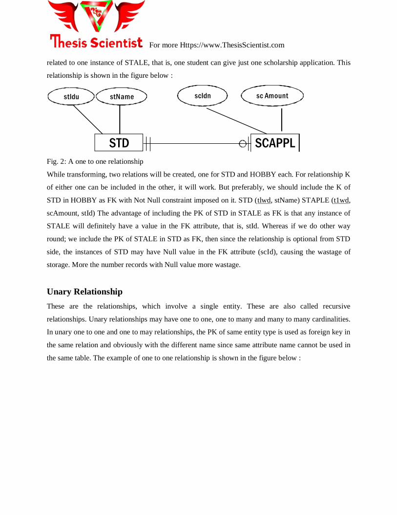
For more Https://www.ThesisScientist.com
related to one instance of STALE, that is, one student can give just one scholarship application. This
relationship is shown in the figure below :
stIdu stName scIdn
STD SCAPPL
sc Amount
Fig. 2: A one to one relationship
While transforming, two relations will be created, one for STD and HOBBY each. For relationship K
of either one can be included in the other, it will work. But preferably, we should include the K of
STD in HOBBY as FK with Not Null constraint imposed on it. STD (tlwd, stName) STAPLE (t1wd,
scAmount, stId) The advantage of including the PK of STD in STALE as FK is that any instance of
STALE will definitely have a value in the FK attribute, that is, stId. Whereas if we do other way
round; we include the PK of STALE in STD as FK, then since the relationship is optional from STD
side, the instances of STD may have Null value in the FK attribute (scId), causing the wastage of
storage. More the number records with Null value more wastage.
Unary Relationship
These are the relationships, which involve a single entity. These are also called recursive
relationships. Unary relationships may have one to one, one to many and many to many cardinalities.
In unary one to one and one to may relationships, the PK of same entity type is used as foreign key in
the same relation and obviously with the different name since same attribute name cannot be used in
the same table. The example of one to one relationship is shown in the figure below :

For more Https://www.ThesisScientist.com
empld empName
MANAGES
ROOMMATE
empAdr
stId stName
EMPLOYEE
STUDENT
STUDENT ( , stName, roommate) _v_E
Fig. 3:One to one relationships (a) one to many (b) one to one and their transformation
In many to many relationships another relation is created with composite key. For example there is
an entity type PART may have many to many recursive relationships, meaning one part consists of
many parts and one part may be used in many parts. So in this case this is a many to many
relationship. The treatment of such a relationship is shown in the figure below :
artId artName
MANAGEPART
PART (pDev_E, partName)SUB-PART (pDev_E2S_c_ c U v)
Super/Subtype Relationship :
Separate relations are created for each super type and subtypes. It means if there is one super type
and there are three subtypes, so then four relations are to be created. After creating these relations
then attributes are assigned. Common attributes are assigned to super type and specialized attributes
are assigned to concerned subtypes. primary key of super type is included in all relations that work
for both link and identity. Now to link the super type with concerned subtype there is a requirement
of descriptive attribute, which is called as discriminator. It is used to identify which subtype is to be
linked. For Example there is an entity type EM which is a super type, now there are three subtypes,
which are salaried, hourly and consultants. So now there is a requirement of a determinant, which can
For more Https://www.ThesisScientist.com
identify that which subtypes to be consulted, so with empId a special character can be added which
can be used to identify the concerned subtype.
Data Manipulation Languages
This is the third component of relational data model. We have studied structure, which is the relation,
integrity constraints both referential and entity integrity constraint. Data manipulation languages are
used to carry out different operations like insertion, deletion or creation of database. Following are
the two types of languages :
Procedural Languages :
These are those languages in which what to do and how to do on the database is required. It means
whatever operation is to be done on the database that has to be told that how to perform.
Non -Procedural Languages :
These are those languages in which only what to do is required, rest how to do is done by the
manipulation language itself.
Structured query language (SQL) is the most widely language used for manipulation of data. But we
will first study Relational Algebra and Relational Calculus, which are procedural and non –
procedural respectively.
Relational Algebra
Following are few major properties of relational algebra :
Relational algebra operations work on one or more relations to deine another relation leaving
the original intact. It means that the input or relational algebra can be one or more relations
and the output would be another relation, but the original participating relations will remain
unchanged and intact. Both operands and results are relations, so output from one operation
can become input to another operation. It means that the input and output both are relations
so they can be used iteratively in different requirements.
Allows expressions to be nested, just as in arithmetic. This property is called closure.
There are five basic operations in relational algebra: Selection, Projection, Cartesian product,
Union, and Set Difference.
These perform most of the data retrieval operations needed.

For more Https://www.ThesisScientist.com
It also has Join, Intersection, and Division operations, which can be expressed in terms of 5
basic operations.
Five Basic Operators of Relational Algebra
In the previous lecture we discussed about the transformation of conceptual database design into
relational database. In E-R data model we had number of constructs but in relational data model it
was only a relation or a table. We started discussion on data manipulation languages (DML) of
relational data model (SDM). We will now study in detail the different operators being used in
relational algebra.
The relational algebra is a procedural query language. It consists of a set of operations that take one
or two relations as input and produce a new relation as their result. There are five basic operations of
relational algebra. They are broadly divided into two categories:
Unary Operations :
These are those operations, which involve only one relation or table. These are Select and project
Binary Operations :
These are those operations, which involve pairs of relations and are, therefore called as binary
operations. The input for these operations is two relations and they produce a new relation without
changing the original relations. These operations are :
Union
Set Difference
Cartesian product
The Select Operation :
The select operation is performed to select certain rows or tuples of a table, so it performs its action
on the table horizontally. The tuples are selected through this operation using a predicate or
condition. This command works on a single table and takes rows that meet a specified condition,
copying them into a new table. Lower Greek letter sigma (σσσσ) is used to denote the selection. The
predicate appears as subscript to P. The argument relation is given in parenthesis following theP. As
a σσresult of this operation a new table is formed, without changing the original table. As a result of
this operation all the attributes of the resulting table are same, which means that degree of the new

For more Https://www.ThesisScientist.com
and old tables are same. Only selected rows / tuples are picked up by the given condition. While
processing a selection all the tuples of a table are looked up and those tuples, which match a
particular condition, are picked up for the new table. The degree of the resulting relation will be the
same as of the relation itself.
| σ | = | r(R) |
The select operation is commutative, which is as under :-
σf (σf(R)) = σf (σf(R))
If a condition 2 (c2) is applied on a relation R and then c1 is applied, the resulting table would be
equivalent even if this condition is reversed that is first c1 is applied and then c2 is applied.
For example there is a table STUDENT with five attributes.
STUDENT
stId stName stAdr prName fcurSem
S1020 Sonam H#14, F/8-4,palwal MCS 4
S1038 narendra H#99, Lala hodal BCS 3
S1015 Tarun H#10, E-8, palwal MCS 5
S1018 ajay E- 2 palwal BIT 5
Fig. 1: An example STDUDENT table
The following is an example of select operation on the table STUDENT :
σnCurr_Sem > 3 (STUDENT)
The components of the select operations are clear from the above example; σ is the symbol being
used (operato), “curr_sem > 3” written in the subscript is the predicate and STUDENT given in
parentheses is the table name. The resulting relation of this command would contain record of those
students whose semester is greater than three as under:
σnCurr_Sem > 3 (STUDENT)
stId stName stAdr prName fcurSem
S1020 Sonam H#14, F/8-4,palwal MCS 4
S1015 narendra H#99, Lala hodal MCS 5
S1018 Tarun H#10, E-8, palwal BIT 5

For more Https://www.ThesisScientist.com
Fig. 2: Output relation of a select operation
In selection operation the comparison operators like <, >, =, <=, >=, <> can be used in the predicate.
Similarly, we can also combine several simple predicates into a larger predicate using the
connectives and (P) and or (P). Some other examples of select operation on the STUDENT table are
given below :
σnstId = „S1015‟ (STUDENT)
σnprName <> „MCS‟ (STUDENT)
The Project Operator
The Select operation works horizontally on the table on the other hand the Project operator operates
on a single table vertically, that is, it produces a vertical subset of the table, extracting the values of
specified columns, eliminating duplicates, and placing the values in a new table. It is unary operation
that returns its argument relation, with certain attributes left out. Since relation is a set any duplicate
rows are eliminated. Projection is denoted by a Greek letter (P). While using this operator all ∏ the
rows of selected attributes of a relation are part of new relation. For example consider a relation
FACULTY with five attributes and certain number of rows.
FACULTY
FacId acName Dept Salary Rank
F2345 Sonam CSE 21000 lecturer
F3456 narendra CSE 23000 Asst Prof
F4567 Tarun ENG 27000 Asst Prof
F5678 Ajay Alhawat MATH 32000 professor
Fig. 3: An example FACULY table
If we apply the projection operator on the table for the following commands all the rows of selected
attributes will be shown, for example :
(FACULTY)
FacId Salary
F2345 21000
F3456 23000
F4567 27000

For more Https://www.ThesisScientist.com
F5678 32000
Fig. 4: Output relation of a project operation on table of figure 3
Some other examples of project operation on the same table can be :
Fname, Rank (Faculty)
Facid, Salary,Rank (Faculty)
Composition of Relational Operators :
The relational operators like select and project can also be used in nested forms iteratively. As the
result of an operation is a relation so this result can be used as an input for other operation. For
Example if we want the names of faculty members along with departments, who are assistant
professors then we have to perform both the select and project operations on the FACULTY table of
figure 3. First selection operator is applied for selecting the associate professors, the operation
outputs a relation that is given as input to the projection operation for the required attributes.
The output of this command will be
acName Dept
NARENDRA CSE
AJAY ENG
Fig. 5: Output relation of nested operations‟ command
We have to be careful about the nested command sequence. For example in the above nested
operations example, if we change the sequence of operations and bring the projection first then the
relation provided to select operation as input will not have the attribute of rank and so then selection
operator can‟t be applied, so there would be an error. So although the sequence can be changed, but
the required attributes should be there either for selection or projection.
The Union Operation :
We will now study the binary operations, which are also called as set operations. The first
requirement for union operator is that the both the relations should be union compatible. It means that
relations must meet the following two conditions:
Both the relations should be of same degree, which means that the number of attributes in
both relations should be exactly same
The domains of corresponding attributes in both the relations should be same. Corresponding
attributes means first attributes of both relations, then second and so on.

For more Https://www.ThesisScientist.com
It is denoted by U. If R and S are two relations, which are union compatible, if we take union of these
two relations then the resulting relation would be the set of tuples either in R or S or both. Since it is
set so there are no duplicate tuples. The union operator is commutative which means :-
R U S = S U R
For Example there are two relations COURSE1 and COURSE2 denoting the two tables storing the
courses being offered at different campuses of an institute? Now if we want to know exactly what
courses are being offered at both the campuses then we will take the union of two tables :
COURSE1
crId C2345 progId 1245 credHrs 3 course Title
C3456 1245 4 Operating Systems Database Systems
C4567 9873 4 Financial Management
C5678 9873 3 Money & Capital Market
COURSE2
crI progId credHrs course Title
C4567 9873 4 Financial Management
C8944 4567 4 Electronics
COURSE1 U COURSE2
crId progId credHrs course Title
C2345 1245 3 Operating Sytems
C3456 1245 4 Database Systems
C4567 9873 4 Financial Management
C5678 9873 3 Money & Capital Market
C8944 4567 4 Electronics
Fig. 5: Two tables and output of union operation on those tables
So in the union of above two courses there are no repeated tuples and they are union compatible as
well.
The Intersection Operation :
The intersection operation also has the requirement that both the relations should be union
compatible, which means they are of same degree and same domains. It is represented byP. If R and

For more Https://www.ThesisScientist.com
S are two relations and we take intersection of these two ∩ relations then the resulting relation would
be the set of tuples, which are in both R and S.
For Example, if we take intersection of COURSE1 and COURSE2 of figure 5 then the resulting
relation would be set of tuples, which are common in both.
COURSE1 )) COURSE2
crId progId credHrs course Title
C4567 9873 4 Financial Management
Fig. 6: Output of intersection operation on COURSE1 and COURSE 2 tables of figure 5
The union and intersection operators are used less as compared to selection and projection operators.
The Set Diference Operator :
If R and S are two relations which are union compatible then difference of these two relations will be
set of tuples that appear in R but do not appear in S. It is denoted by (-) for example if we apply
difference operator on Course1 and Course2 then the resulting relation would be as under :
COURSE1 – COURSE2
CID ProgID Cred_Hrs Course Title
C2345 1245 3 Operating Systems
C3456 1245 4 Database Systems
C5678 9873 3 Money & Capital Market
Fig. 7: Output of difference operation on COURSE1 and COURSE 2 tables of figure 5
Cartesian product :
The Cartesian product needs not to be union compatible. It means they can be of different degree. It
is denoted by X. suppose there is a relation R with attributes (A1, A2,...An) and S with attributes
(B1, B2……B). The Cartesian product will be :
R X S
The resulting relation will be containing all the attributes of R and all of S. Moreover, all the rows of
R will be merged with all the rows of S. So if there are m attributes and C rows in R and n attributes
and D rows in S then the relations R x S will contain m + n columns and C * D rows. It is also called
as cross product. The Cartesian product is also commutative and associative. For Example there are
two relations COURSE and

For more Https://www.ThesisScientist.com
COURSE X STUDENT
crId course Title stId stName
C3456 Database Systems S101 ajay
C4567 Financial Management S101 ajay
C5678 Money & Capital Market S101 ajay
C3456 Database Systems S103 narendra
C4567 Financial Management S103 narendra
C5678 Money & Capital Market S103 narendra
Fig. 7: Input tables and output of Cartesian product
Join Operation :
Join is a special form of cross product of two tables. In Cartesian product we join a tuple of one table
with the tuples of the second table. But in join there is a special requirement of relationship between
tuples. For example if there is a relation STUDENT and a relation BOOK then it may be required to
know that how many books have been issued to any particular student. Now in this case the primary
key of STUDENT that is stId is a foreign key in BOOK table through which the join can be made.
Types of Joins
Join is a special form of cross product of two tables. It is a binary operation that allows combining
certain selections and a Cartesian product into one operation. The join operation forms a Cartesian
product of its two arguments, performs a selection forcing equality on those attributes that appear in
both relation schemas, and finally removes duplicate attributes. Following are the different types of
joins :
1. Theta Join
2. PEqui Join
3. PSemi Join
4. PNatural Join
5. POuter Joins
We will now discuss them one by one
Theta Join :

For more Https://www.ThesisScientist.com
In theta join we apply the condition on input relation(s) and then only those selected rows are used in
the cross product to be merged and included in the output. It means that in normal cross product all
the rows of one relation are mapped/merged with all the rows of second relation, but here only
selected rows of a relation are made cross product with second relation. It is denoted as under :-
If R and S are two relations then Pis the condition, which is applied for select operation on one
relation and then only selected rows are cross product with all the rows of second relation. For
Example there are two relations of FACULTY and COURSE, now we will first apply select
operation on the FACULTY relation for selection certain specific rows then these rows will have
across product with COURSE relation, so this is the difference in between cross product and theta
join. We will now see first both the relation their different attributes and then finally the cross
product after carrying out select operation on relation.
From this example the difference in between cross product and theta join becomes clear.
FACULTY
acid acName dept salary rank
F234 Sonam CSE 21000 lecturer
F235 narendra CSE 23000 Asso rof
F236 Tarun ENG 27000 Asso Prof
F237 Ajay Alhawat ENG 32000 Professor
COURSE
crCode crTitle Id
C3456 Database Systems F234
C3457 Financial Management
C3458 Money & Capital Market F236
C3459 Introduction to Accounting F237
(σ rank = „Asso Prof‟(FACULTY)) X COURSE
acId ac Name f dept f salary rank cr Code fcr Title Id
F235 Tahir CSE 23000 Assorof C3456 Database Systems F234
F235 Tahir CSE 23000 Assorof C3457 Financial Management
F235 Tahir CSE 23000 Assorof C3458 Money & Capital Market P F236
F235 Tahir CSE 23000 Assorof C3459 Introduction to Accounting F237
F236 Ayesha ENG P27000 Assorof C3456 Database Systems F234
F236 Ayesha ENG P 27000 Assorof C3457 Financial Management
F236 Ayesha ENG P 27000 Assorof C3458 Money & Capital Market P F236

For more Https://www.ThesisScientist.com
F236 Ayesha ENG P 27000 Assorof C3459 Introduction to Accounting F237
Fig. 1: Two tables with an example of theta join In this example after fulfilling the select condition of
Associate professor on faculty relation then it is cross product with course relation
Equi–Join :
This is the most used type of join. In equi–join rows are joined on the basis of values of a common
attribute between the two relations. It means relations are joined on the basis of common attributes
between them; which are meaningful. This means on the basis of primary key, which is a foreign key
in another relation. Rows having the same value in the common attributes are joined. Common
attributes appear twice in the output. It means that the attributes, which are common in both relations,
appear twice, but only those rows, which are selected. Common attribute with the same name is
qualified with the relation name in the output. It means that if primary and foreign keys of two
relations are having the same names and if we take the equi – join of both then in the output relation
the relation name will precede the attribute name. For Example, if we take the equi – join of faculty
and course relations then the output would be as under :-
FACULTY
COURSE
acid ac Name f dept Salary
f
rank cr Code fcr Title ID
F234 Sonam CSE 21000 lecturer C3456 Database Systems F234
F236 narendra ENG 27000 Asso Prof P C3458 Money & Capital
Market
F236
F237 Tarun ENG 32000 Professor C3459 Introduction to A/c F237
Fig. 2: Equi-join on tables of figure 1
In the above example the name of common attribute between the two tables is different, that is, it is
facId in FACULTY and fId in COURSE, so it is not required to qualify; however there is no harm
doing it still. Now in this example after taking equi–join only those tuples are selected in the output
whose values are common in both the relations.
Natural Join :

For more Https://www.ThesisScientist.com
This is the most common and general form of join. If we simply say join, it means the natural join. It
is same as equi–join but the difference is that in natural join, the common attribute appears only once.
Now, it does not matter which common attribute should be part of the output relation as the values in
both are same. For Example if we take the natural join of faculty and course the output would be as
under :-
FACULTY COURSE
acid ac Name f dept salary rank cr Code fcr Title
F234 Sonam CSE 21000 Lecturer C3456 Database Systems
F236 narendra ENG 27000 Asso Prof C3458 Money & Capital Market
F237 Tarun ENG 32000 Professor C3459 Introduction to Accounting
Fig. 4: Natural join o FACULTY and COURSE tables of figure 1
In this example the common attribute appears only once, rest the behavior is same. Following are the
different types of natural join:-
Left Outer Join :
In left outer join all the tuples of left relation remain part of the output. The tuples that have a
matching tuple in the second relation do have the corresponding tuple from the second relation.
However, for the tuples of the left relation, which do not have a matching record in the right tuple
have Null values against the attributes of the right relation. The example is given in figure 5 below. It
can be described in another way. Left outer join is the equi-join plus the non matching rows of the
left side relation having Null against the attributes of right side relation.
Right Outer Join :
In right outer join all the tuples of right relation remain part of the output relation, whereas on the left
side the tuples, which do not match with the right relation, are left as null. It means that right outer
join will always have all the tuples of right relation and those tuples of left relation which are not
matched are left as Null.

For more Https://www.ThesisScientist.com
Fig. 5: Input tables and left outer join and right outer join
Outer Join :
In outer join all the tuples of left and right relations are part of the output. It means that all those
tuples of left relation which are not matched with right relation are left as Null. Similarly all those
tuples of right relation which are not matched with left relation are left as Null.
Fig. 6: outer join operation on tables of figure 5
Semi Join :
In semi join, first we take the natural join of two relations then we project the attributes of first table
only. So after join and matching the common attribute of both relations only attributes of first
relation are projected. For Example if we take the semi join of two relations faculty and course then
the resulting relation would be as under:-
FACULTY COURSE

For more Https://www.ThesisScientist.com
acid ac Name f Dept Salary Rank
F234 Sonam CSE 21000 lecturer
F236 narendra ENG 27000 Asso Prof
F237 Tarun ENG 32000 Professor
Fig. 7: Semi-join operation on tables of figure 1
Now the resulting relation has attributes of first relation only after taking the natural join of both
relations.
Relational Calculus
Relational Calculus is a nonprocedural formal relational data manipulation language in which the
user simply specifies what data should be retrieved, but not how to retrieve it. It is an alternative
standard for relational data manipulation languages. The relational calculus is not related to the
familiar differential and integral calculus in mathematics, but takes its name from a branch of
symbolic logic called the predicate calculus. It has two following two forms :-
Tuple Oriented Relational Calculus
Domain Oriented Relational Calculus
Tuple Oriented Relational Calculus :
In tuple oriented relational calculus we are interested primarily in finding relation tuples for which a
predicate is true. To do so we need tuple variables. A tuple variable is a variable that takes on only
the tuples of some relation or relations as its range of values. It actually corresponds to a
mathematical domain. We specify the range of a tuple variable by a statement such as :-
RANGE OF S IS STUDENT
Here, S is the tuple variable and STUDENT is the range, so that S always represents a tuple of
STUDENT. It is expressed as {S | (S)} We will read it as find the set of all tuples S such that P(S) is
true, where P implies the predicate condition now suppose range of R is STUDENT {R | R.Credits >
50} We will say like find the stuId, stuName, majors etc of all students having more than 50 credits.
Domain Oriented Relational Calculus :
Normalization
For more Https://www.ThesisScientist.com
There are four types of anomalies, which are of concern, redundancy, insertion, deletion and
updation. Normalization is not compulsory, but it is strongly recommended that normalization must
be done. Because normalized design makes the maintenance of database much easier. While carrying
out the process of normalization, it should be applied on each table of database. It is performed after
the logical database design. This process is also being followed informally during conceptual
database design as well.
Normalization Process
There are different forms or levels of normalization. They are called as first, second and so on. Each
normalized form has certain requirements or conditions, which must be fulfilled. If a table or relation
fulfills any particular form then it is said to be in that normal form. The process is applied on each
relation of the database. The minimum form in which all the tables are in is called the normal form of
entire database. The main objective of normalization is to place the database in highest form of
normalization.
Functional Dependency
Normalization is based on the concept of functional dependency. A functional dependency is a type
of relationship between attributes.
Definition o Functional Dependency
If A and B are attributes or sets of attributes of relation R, we say that B is functionally dependent on
A if each value of A in R has associated with it exactly one value of B in R. W
e write this as A B, read as “A functionally determines B” or “ A determines B”. This does not
mean that A causes B or that the value of B can be calculated from the value of A by a formula,
although sometimes that is the case. It simply means that if we know the value of A and we examine
the table of relation R, we will find only one value of B in all the rows that have the given value of A
at any one time. Thus then the two rows have the same A value, they must also have the same B
value. However, for a given B value, there may be several different A values. When a functional
dependency exits, the attributes or set of attributes on the left side of the arrow is called a
determinant. Attribute of set of attributes on left side are called determinant and on right are called
dependants. If there is a relation R with attributes (a,b,c,d,e) a, b, c, d, e)

For more Https://www.ThesisScientist.com
For Example there is a relation of student with following attributes. We will establish the functional
dependency of different attributes :-
Now in this example if we know the stID we can tell the complete information about that student.
Similarly if we know the prName , we can tell the credit hours for any particular subject.
Functional Dependencies and Keys :
We can determine the keys of a relation after seeing its functional dependencies. The determinant of
functional dependency that determines all attributes of that table is the super key. Super key is an
attribute or a set of attributes that identifies an entity uniquely. In a table, a super key is any column
or set of columns whose values can be used to distinguish one row from another. A minimal super
key is the candidate key, so if a determinant of functional ependency determines all attributes of that
relation then it is definitely a super key and if there is no other functional dependency whereas a
subset of this determinant is a super key then it is a candidate key. So the functional dependencies
help to identify keys. We have an example as under :-
EMP (eId,eName,eAdr,eDept,prId,prSal)
eId (eName,eAdr,eDept)
eId,prId prSal
Now in this example in the employee relation eId is the key from which we can uniquely determine
the employee name address and department . Similarly if we know the employee ID and project ID
we can find the project salary as well. So FDs help in finding out the keys and their relation as well.
Normal Forms
Normalization is basically; a process of efficiently organizing data in a database. There are two goals
of the normalization process: eliminate redundant data (for example, storing the same data in more
than one table) and ensure data dependencies make sense (only storing related data in a table). Both
of these are worthy goals as they reduce the amount of space a database consumes and ensure that
data is logically stored. We will now study the first normal.

For more Https://www.ThesisScientist.com
First Normal Form :
A relation is in first normal form if and only if every attribute is single valued for each tuple. This
means that each attribute in each row , or each cell of the table, contains only one value. No repeating
fields or groups are allowed. An alternative way of describing first normal form is to say that the
domains of attributes of a relation are atomic, that is they consist of single units that cannot be broken
down further. There is no multivalued (repeating group) in the relation multiple values create
problems in performing operations like select or join. For Example there is a relation of Student
STD(stIdstName,stAdr,prName,bkId)
stId stName stAdr prName bkId
S1020 Sonam I-8 palwal Mcs B00129
S1038 narendra G-6 faridabad PBCS B00327
S1015 Tarun L hodal MCS B08945, B06352
S1018 Ajay
Alhawat
E-8, palwal BIT B08474
Now in this table there is no unique value for every tuple, like for S1015 there are two values for
bookId. So to bring it in the first normal form.
stId stName stAdr prName bkId
S1020 Sonam I-8 palwal MCS B00129
S1038 narendra G-6 faridabad PBCS B00327
S1015 Tarun L hodal MCS B08945
S1015 Ajay Alhawat E-8, palwal MCS B06352
S1018 ritu palwal BIT B08474
Now this table is in first normal form and for every tuple there is a unique value. Second Normal
Form :
A relation is in second normal form (2NF) if and only if it is in first normal form and all the nonkey
attributes are fully functionally dependent on the key. Clearly, if a relation is in 1NF and the key
consists of a single attribute, the relation is automatically in 2NF. The only time we have to be
concerned about 2NF is when the key is composite. Second normal form (2NF) addresses the
concept of removing duplicative data. It remove subsets of data that apply to multiple rows of a table

For more Https://www.ThesisScientist.com
and place them in separate tables. It creates relationships between these new tables and their
predecessors through the use of foreign keys.
Second Normal Form
A relation is in second normal form if and only if it is in first normal form and all nonkey attributes
are fully functionally dependent on the key. Clearly if a relation is in 1NF and the key consists of a
single attribute, the relation is automatically 2NF.
The only time we have to be concerned 2NF is when the key is composite. A relation that is not in
2NF exhibits the update, insertion and deletion anomalies we will now see it with an example.
Consider the following relation.
Now in this relation the key is course ID and student ID. The requirement of 2NF is that all non-key
attributes should be fully dependent on the key there should be no partial dependency of the
attributes. But in this relation student ID is dependent on student name and similarly course ID is
partially dependent on faculty ID and room, so it is not in second normal form. At this level of
normalization, each column in a table that is not a determiner of the contents of another column must
itself be a function of the other columns in the table. For example, in a table with three columns
containing customer ID, product sold, and price of the product when sold, the price would be a
function of the customer ID (entitled to a discount) and the specific product. If a relation is not in
2NF then there are some anomalies, which are as under:
Redundancy
Insertion Anomaly
Deletion Anomaly
Updation Anomaly
The general requirements of 2NF are:-
Remove subsets of data that apply to multiple rows of a table and place them in separate
rows.
Create relationships between these new tables and their predecessors through the use of
foreign keys.
Consider the following table which has the anomalies :-
crId StId stName Id room grade
C3456 S1020 Sonam F2345 104 B

For more Https://www.ThesisScientist.com
C5678 S1020 narendra F4567 106
C3456 S1038 Tarun F2345 104 A
C5678 S1015 Ajay
Alhawat
F4567 106 B
Now the first thing is that the table is in 1NF because there are no duplicate values in any tuple and
all cells contain atomic value. The first thing is the redundancy. Like in this table of CLASS the
course ID C3456 is being repeated for faculty ID F2345 and similarly the room no 104 is being
repeated twice. Second is the insertion anomaly. Suppose we want to insert a course in the table, but
this course has not been registered to any student. But we cannot enter the student ID, because no
student has registered this course yet. So we can also not insert this course. This is called as insertion
anomaly which is wrong state of database. Next is the deletion anomaly. Suppose there is a course
which has been enrolled by one student only. Now due to some reason, we want to delete the record
of student. But here the information about the course will also be deleted, so in this way this is the
incorrect state of database in which infact we want to delete the information about the student record
but along with this the course information has also been deleted. So it is not reflecting the actual
system.
Now the next is updation anomaly. Suppose a course has been registered by 50 students and now we
want to change the class rooms of all the students. So in this case we will have to change the records
of all the 50 students. So this is again a deletion anomaly.The process for transforming a 1NF table to
2NF is:
Identify any determinants other than the composite key, and the columns they determine.
Create and name a new table for each determinant and the unique columns it determines.
Move the determined columns from the original table to the new table. The determinate
becomes the primary key of the new table.
Delete the columns you just moved from the original table except for the determinant which
will serve as a foreign key.
The original table may be renamed to maintain semantic meaning.
Third Normal Form

For more Https://www.ThesisScientist.com
A relational table is in third normal form (3NF) if it is already in 2NF and every non-key column is
non-transitively dependent upon its primary key. In other words, all nonkey attributes are
functionally dependent only upon the primary key.
The process of transforming a table into 3NF is:
Identify any determinants, other the primary key, and the columns they determine.
Create and name a new table for each determinant and the unique columns it determines.
Move the determined columns from the original table to the new table. The determinate
becomes the primary key of the new table.
Delete the columns you just moved from the original table except for the determinate which
will serve as a foreign key.
The original table may be renamed to maintain semantic meaning.
Higher Normal Forms
After BCNF are the fourth, a fifth and domain key normal form exists. Although till BCNF normal
form tables are in required form, but if we want we can move on to fourth and fifth normal forms as
well. 4NF deals with multivalued dependency, fifth deals with possible loss less decompositions;
DKNF reduces further chances of any possible inconsistency.


![MATH-8 Exam [E-1HYETD] Relations and Functions](https://static.fdocuments.net/doc/165x107/61d898b62edf8e458c39ac87/math-8-exam-e-1hyetd-relations-and-functions.jpg)
