Data Mining with R Regression models

Hamideh Iraj

Hamideh.iraj@ut.ac.ir

Slides Reference

This a curation from:

Data Analysis Course

Weeks 4-5-6

https://www.coursera.org/course/dataanalysis

Galton Data – Introduction

library(UsingR)data(galton)

----------------------------------Head(galton)Tail(galton)

----------------------------------Dim(galton)Str(galton)summary(galton)summary(galton$child)

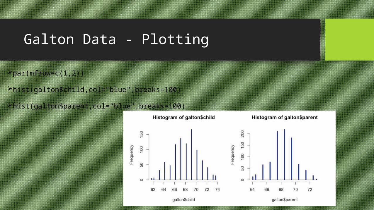
Galton Data - Plotting

par(mfrow=c(1,2))

hist(galton$child,col="blue",breaks=100)

hist(galton$parent,col="blue",breaks=100)

Galton Data – Plotting - cont.

pairs(galton)

What is Regression Analysis?

regression analysis is a statistical process for estimating the relationships among variables. It includes many techniques for modeling and analyzing several variables, when the focus is on the relationship between a dependent variable and one or more independent variables.

http://en.wikipedia.org/wiki/Regression_analysis

Fitting a line

plot(galton$child, galton$parent,

pch=19,col="blue")

lm1 <- lm(child ~ parent, data=galton)

lines(galton$parent,lm1$fitted,col="red",

lwd=3)

The line width

Plot Residuals

plot(galton$parent,lm1$residuals,col="blue",pch=19)Abline (c(0,0),col="red",lwd=3)

Linear Model Coefficients

>Summary(lm1) lm1$coeff

Why care about model Accuracy?

http://en.wikipedia.org/wiki/Linear_regression

Model Accuracy Measures

P-value

Confidence Interval

R2

Adjusted R2

P-value

Most Common Measure of Statistical Significance

Idea: Suppose nothing is going on - how unusual is it to see the estimate we

got?

Some typical values (single test)

P < 0.05 (significant)

P < 0.01 (strongly significant)

P < 0.001 (very significant)

Confidence intervals

A confidence interval is a type of interval estimate of a population parameter and is used to indicate the reliability of an estimate

confint(lm1,level=0.95)

http://en.wikipedia.org/wiki/Confidence_interval

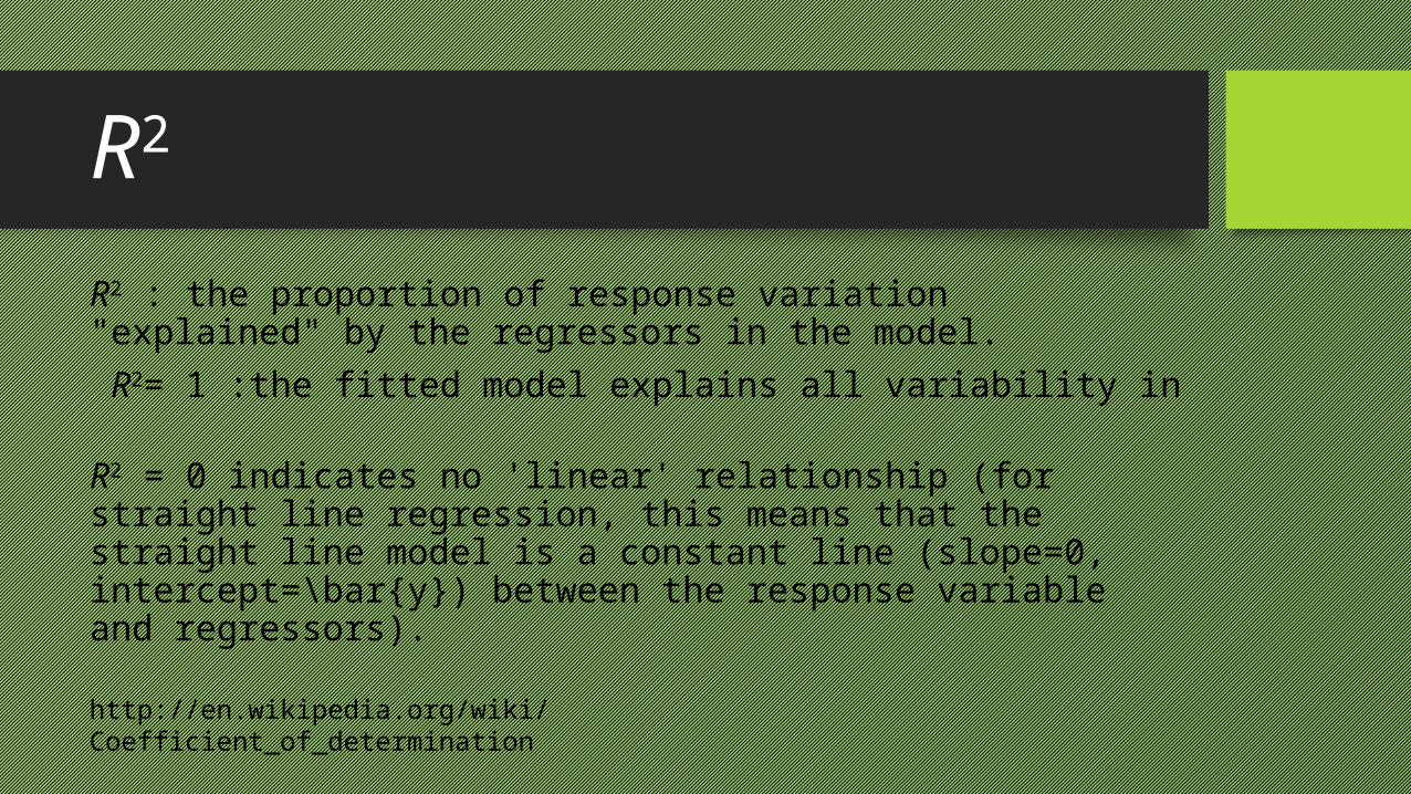
R2

R2 : the proportion of response variation "explained" by the regressors in the model.

R2= 1 :the fitted model explains all variability in

R2 = 0 indicates no 'linear' relationship (for straight line regression, this means that the straight line model is a constant line (slope=0, intercept=\bar{y}) between the response variable and regressors).

http://en.wikipedia.org/wiki/Coefficient_of_determination

Adjusted R2

The use of an adjusted R2 (often written as \bar R^2 and

pronounced "R bar squared") is an attempt to take account

of the phenomenon of the R2 automatically and spuriously

increasing when extra explanatory variables are added to

the model.

http://en.wikipedia.org/wiki/Coefficient_of_determination

Predicting with Linear Regression

coef(lm1)[1] + coef(lm1)[2]*80

newdata <- data.frame(parent=80)

predict(lm1,newdata)

Multivariate Linear Regression

WHO childhood hunger data

Dataset: http://apps.who.int/gho/athena/data/GHO/WHOSIS_000008.csv?profile=text&filter=COUNTRY:*

hunger <- read.csv("./hunger.csv")

hunger <- hunger[hunger$Sex!="Both sexes", ]

Multivariate Linear Regression – cont.

lmBoth <- lm(hunger$Numeric ~ hunger$Year + hunger$Sex)

lmBoth2 <- lm(hunger$Numeric ~ hunger$Year + hunger$Sex + hunger$Sex*hunger$Year)

Same slopes

Different slopes

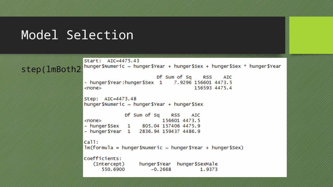
Model Selection

step(lmBoth2)

Regression with Factor Variables

Outcome is still quantitative Covariate(s) are factor variables Fitting lines = fitting means Want to evaluate contribution of all factor levels at once

Regression with Factor Variables – cont.

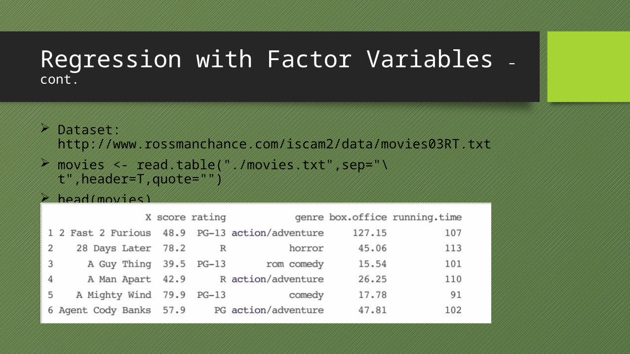
Dataset: http://www.rossmanchance.com/iscam2/data/movies03RT.txt movies <- read.table("./movies.txt",sep="\t",header=T,quote="") head(movies)

Regression with Factor Variables – cont.

lm2 <- lm(movies$score ~ as.factor(movies$rating)) summary(lm2)