Data Mining:5. Algoritma Klastering

Romi Satria Wahonoromi@romisatriawahono.net

http://romisatriawahono.net/dmWA/SMS: +6281586220090

1

Romi Satria Wahono

• SD Sompok Semarang (1987)• SMPN 8 Semarang (1990)• SMA Taruna Nusantara Magelang (1993)• B.Eng, M.Eng and Ph.D in Software Engineering from

Saitama University Japan (1994-2004)Universiti Teknikal Malaysia Melaka (2014)

• Research Interests: Software Engineering,Machine Learning

• Founder dan Koordinator IlmuKomputer.Com• Peneliti LIPI (2004-2007)• Founder dan CEO PT Brainmatics Cipta Informatika

2

Course Outline

1. Pengantar Data Mining

2. Proses Data Mining

3. Persiapan Data

4. Algoritma Klasifikasi

5. Algoritma Klastering

6. Algoritma Asosiasi

7. Algoritma Estimasi

3

5. Algoritma Klastering5.1 Cluster Analysis: Basic Concepts

5.2 Partitioning Methods

5.3 Hierarchical Methods

5.4 Density-Based Methods

5.5 Grid-Based Methods

5.6 Evaluation of Clustering4

5.1 Cluster Analysis: Basic Concepts

5

What is Cluster Analysis?

• Cluster: A collection of data objects• similar (or related) to one another within the same group• dissimilar (or unrelated) to the objects in other groups

• Cluster analysis (or clustering, data segmentation, …)• Finding similarities between data according to the

characteristics found in the data and grouping similar data objects into clusters

• Unsupervised learning: no predefined classes (i.e., learning by observations vs. learning by examples: supervised)

• Typical applications• As a stand-alone tool to get insight into data distribution • As a preprocessing step for other algorithms

6

Applications of Cluster Analysis• Data reduction

• Summarization: Preprocessing for regression, PCA, classification, and association analysis

• Compression: Image processing: vector quantization• Hypothesis generation and testing• Prediction based on groups

• Cluster & find characteristics/patterns for each group

• Finding K-nearest Neighbors• Localizing search to one or a small number of clusters

• Outlier detection: Outliers are often viewed as those “far away” from any cluster

7

Clustering: Application Examples• Biology: taxonomy of living things: kingdom, phylum, class,

order, family, genus and species• Information retrieval: document clustering• Land use: Identification of areas of similar land use in an earth

observation database• Marketing: Help marketers discover distinct groups in their

customer bases, and then use this knowledge to develop targeted marketing programs

• City-planning: Identifying groups of houses according to their house type, value, and geographical location

• Earth-quake studies: Observed earth quake epicenters should be clustered along continent faults

• Climate: understanding earth climate, find patterns of atmospheric and ocean

• Economic Science: market research8

Basic Steps to Develop a Clustering Task• Feature selection

• Select info concerning the task of interest• Minimal information redundancy

• Proximity measure• Similarity of two feature vectors

• Clustering criterion• Expressed via a cost function or some rules

• Clustering algorithms• Choice of algorithms

• Validation of the results• Validation test (also, clustering tendency test)

• Interpretation of the results• Integration with applications

9

Quality: What Is Good Clustering?• A good clustering method will produce high quality

clusters• high intra-class similarity: cohesive within clusters• low inter-class similarity: distinctive between clusters

• The quality of a clustering method depends on• the similarity measure used by the method • its implementation, and• Its ability to discover some or all of the hidden patterns

10

Measure the Quality of Clustering• Dissimilarity/Similarity metric

• Similarity is expressed in terms of a distance function, typically metric: d(i, j)

• The definitions of distance functions are usually rather different for interval-scaled, boolean, categorical, ordinal ratio, and vector variables

• Weights should be associated with different variables based on applications and data semantics

• Quality of clustering:• There is usually a separate “quality” function that

measures the “goodness” of a cluster.• It is hard to define “similar enough” or “good enough”

• The answer is typically highly subjective

11

Considerations for Cluster Analysis• Partitioning criteria

• Single level vs. hierarchical partitioning (often, multi-level hierarchical partitioning is desirable)

• Separation of clusters• Exclusive (e.g., one customer belongs to only one region) vs. non-

exclusive (e.g., one document may belong to more than one class)

• Similarity measure• Distance-based (e.g., Euclidian, road network, vector) vs.

connectivity-based (e.g., density or contiguity)

• Clustering space• Full space (often when low dimensional) vs. subspaces (often in

high-dimensional clustering)

12

Requirements and Challenges• Scalability

• Clustering all the data instead of only on samples

• Ability to deal with different types of attributes• Numerical, binary, categorical, ordinal, linked, and mixture of these

• Constraint-based clustering• User may give inputs on constraints• Use domain knowledge to determine input parameters

• Interpretability and usability• Others

• Discovery of clusters with arbitrary shape• Ability to deal with noisy data• Incremental clustering and insensitivity to input order• High dimensionality

13

Major Clustering Approaches 1• Partitioning approach:

• Construct various partitions and then evaluate them by some criterion, e.g., minimizing the sum of square errors

• Typical methods: k-means, k-medoids, CLARANS

• Hierarchical approach: • Create a hierarchical decomposition of the set of data (or

objects) using some criterion• Typical methods: Diana, Agnes, BIRCH, CAMELEON

• Density-based approach: • Based on connectivity and density functions• Typical methods: DBSACN, OPTICS, DenClue

• Grid-based approach: • based on a multiple-level granularity structure• Typical methods: STING, WaveCluster, CLIQUE

14

Major Clustering Approaches 2• Model-based:

• A model is hypothesized for each of the clusters and tries to find the best fit of that model to each other

• Typical methods: EM, SOM, COBWEB

• Frequent pattern-based:• Based on the analysis of frequent patterns• Typical methods: p-Cluster

• User-guided or constraint-based: • Clustering by considering user-specified or application-specific

constraints• Typical methods: COD (obstacles), constrained clustering

• Link-based clustering:• Objects are often linked together in various ways• Massive links can be used to cluster objects: SimRank, LinkClus

15

5.2 Partitioning Methods

16

Partitioning Algorithms: Basic Concept• Partitioning method: Partitioning a database D of n objects

into a set of k clusters, such that the sum of squared distances is minimized (where ci is the centroid or medoid of cluster Ci)

• Given k, find a partition of k clusters that optimizes the chosen partitioning criterion

• Global optimal: exhaustively enumerate all partitions• Heuristic methods: k-means and k-medoids algorithms• k-means (MacQueen’67, Lloyd’57/’82): Each cluster is represented by the

center of the cluster• k-medoids or PAM (Partition around medoids) (Kaufman & Rousseeuw’87):

Each cluster is represented by one of the objects in the cluster

17

21 )),(( iCp

ki cpdE

i

The K-Means Clustering Method

• Given k, the k-means algorithm is implemented in four steps:

1. Partition objects into k nonempty subsets

2. Compute seed points as the centroids of the clusters of the current partitioning (the centroid is the center, i.e., mean point, of the cluster)

3. Assign each object to the cluster with the nearest seed point

4. Go back to Step 2, stop when the assignment does not change

18

An Example of K-Means Clustering

19

K=2

Arbitrarily partition objects into k groups

Update the cluster centroids

Update the cluster centroids

Reassign objectsLoop if needed

The initial data set

Partition objects into k nonempty subsets

Repeat Compute centroid (i.e., mean

point) for each partition Assign each object to the

cluster of its nearest centroid Until no change

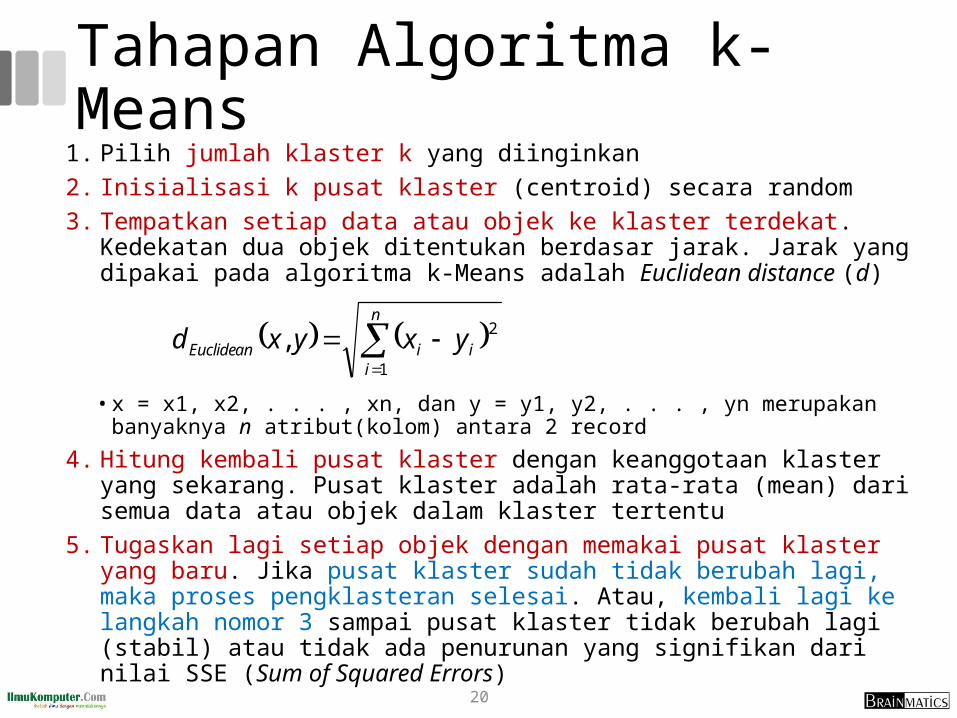
Tahapan Algoritma k-Means

1. Pilih jumlah klaster k yang diinginkan 2. Inisialisasi k pusat klaster (centroid) secara random3. Tempatkan setiap data atau objek ke klaster terdekat. Kedekatan dua objek

ditentukan berdasar jarak. Jarak yang dipakai pada algoritma k-Means adalah Euclidean distance (d)

• x = x1, x2, . . . , xn, dan y = y1, y2, . . . , yn merupakan banyaknya n atribut(kolom) antara 2 record

4. Hitung kembali pusat klaster dengan keanggotaan klaster yang sekarang. Pusat klaster adalah rata-rata (mean) dari semua data atau objek dalam klaster tertentu

5. Tugaskan lagi setiap objek dengan memakai pusat klaster yang baru. Jika pusat klaster sudah tidak berubah lagi, maka proses pengklasteran selesai. Atau, kembali lagi ke langkah nomor 3 sampai pusat klaster tidak berubah lagi (stabil) atau tidak ada penurunan yang signifikan dari nilai SSE (Sum of Squared Errors) 20

n

iiiEuclidean yxyxd

1

2,

Contoh Kasus – Iterasi 1

1. Tentukan jumlah klaster k=2

2. Tentukan centroid awal secara acak misal dari data disamping m1 =(1,1), m2=(2,1)

3. Tempatkan tiap objek ke klaster terdekat berdasarkan nilai centroid yang paling dekat selisihnya (jaraknya). Didapatkan hasil, anggota cluster1 = {A,E,G}, cluster2={B,C,D,F,H}

Nilai SSE yaitu:

21

2

1

,

k

i Cpi

i

mpdSSE

Interasi 2

22

2,13/123,3/1111 m

4,2;6,35/12333,5/245432 m

4. Menghitung nilai centroid yang baru

5. Tugaskan lagi setiap objek dengan memakai pusat klaster yang baru.

Nilai SSE yang baru:

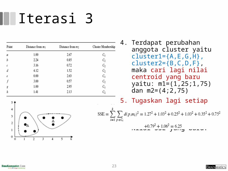
Iterasi 3

4. Terdapat perubahan anggota cluster yaitu cluster1={A,E,G,H}, cluster2={B,C,D,F}, maka cari lagi nilai centroid yang baru yaitu: m1=(1,25;1,75) dan m2=(4;2,75)

5. Tugaskan lagi setiap objek dengan memakai pusat klaster yang baruNilai SSE yang baru:

23

Hasil Akhir

• Dapat dilihat pada tabel. Tidak ada perubahan anggota lagi pada masing-masing cluster

• Hasil akhir yaitu: cluster1={A,E,G,H}, dan cluster2={B,C,D,F}Dengan nilai SSE = 6,25 dan jumlah iterasi 3

24

Comments on the K-Means Method• Strength:

• Efficient: O(tkn), where n is # objects, k is # clusters, and t is # iterations. Normally, k, t << n.

• Comparing: PAM: O(k(n-k)2 ), CLARA: O(ks2 + k(n-k))

• Comment: Often terminates at a local optimal

• Weakness• Applicable only to objects in a continuous n-dimensional space

• Using the k-modes method for categorical data

• In comparison, k-medoids can be applied to a wide range of data

• Need to specify k, the number of clusters, in advance (there are ways to automatically determine the best k (see Hastie et al., 2009)

• Sensitive to noisy data and outliers

• Not suitable to discover clusters with non-convex shapes

25

Variations of the K-Means Method• Most of the variants of the k-means which differ in

• Selection of the initial k means• Dissimilarity calculations• Strategies to calculate cluster means

• Handling categorical data: k-modes• Replacing means of clusters with modes• Using new dissimilarity measures to deal with categorical

objects• Using a frequency-based method to update modes of

clusters• A mixture of categorical and numerical data: k-prototype

method26

What Is the Problem of the K-Means Method?• The k-means algorithm is sensitive to outliers!

• Since an object with an extremely large value may substantially distort the distribution of the data

• K-Medoids: • Instead of taking the mean value of the object in a cluster as a

reference point, medoids can be used, which is the most centrally located object in a cluster

27

0

1

2

3

4

5

6

7

8

9

10

0 1 2 3 4 5 6 7 8 9 10

0

1

2

3

4

5

6

7

8

9

10

0 1 2 3 4 5 6 7 8 9 10

28

PAM: A Typical K-Medoids Algorithm

0

1

2

3

4

5

6

7

8

9

10

0 1 2 3 4 5 6 7 8 9 10

Total Cost = 20

0

1

2

3

4

5

6

7

8

9

10

0 1 2 3 4 5 6 7 8 9 10

K=2

Arbitrary choose k object as initial medoids

0

1

2

3

4

5

6

7

8

9

10

0 1 2 3 4 5 6 7 8 9 10

Assign each remaining object to nearest medoids Randomly select a

nonmedoid object,Oramdom

Compute total cost of swapping

0

1

2

3

4

5

6

7

8

9

10

0 1 2 3 4 5 6 7 8 9 10

Total Cost = 26

Swapping O and Oramdom

If quality is improved.

Do loop

Until no change

0

1

2

3

4

5

6

7

8

9

10

0 1 2 3 4 5 6 7 8 9 10

The K-Medoid Clustering Method• K-Medoids Clustering: Find representative objects

(medoids) in clusters• PAM (Partitioning Around Medoids, Kaufmann &

Rousseeuw 1987)• Starts from an initial set of medoids and iteratively replaces

one of the medoids by one of the non-medoids if it improves the total distance of the resulting clustering

• PAM works effectively for small data sets, but does not scale well for large data sets (due to the computational complexity)

• Efficiency improvement on PAM• CLARA (Kaufmann & Rousseeuw, 1990): PAM on samples• CLARANS (Ng & Han, 1994): Randomized re-sampling

29

5.3 Hierarchical Methods

30

Hierarchical Clustering• Use distance matrix as clustering criteria• This method does not require the number of clusters k as an

input, but needs a termination condition

31

Step 0 Step 1 Step 2 Step 3 Step 4

b

d

c

e

aa b

d e

c d e

a b c d e

Step 4 Step 3 Step 2 Step 1 Step 0

agglomerative(AGNES)

divisive(DIANA)

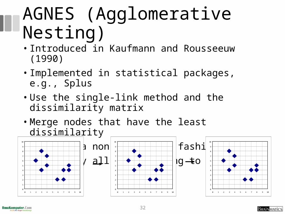
AGNES (Agglomerative Nesting)• Introduced in Kaufmann and Rousseeuw (1990)• Implemented in statistical packages, e.g., Splus• Use the single-link method and the dissimilarity matrix • Merge nodes that have the least dissimilarity• Go on in a non-descending fashion• Eventually all nodes belong to the same cluster

32

0

1

2

3

4

5

6

7

8

9

10

0 1 2 3 4 5 6 7 8 9 10

0

1

2

3

4

5

6

7

8

9

10

0 1 2 3 4 5 6 7 8 9 10

0

1

2

3

4

5

6

7

8

9

10

0 1 2 3 4 5 6 7 8 9 10

Dendrogram: Shows How Clusters are Merged

33

Decompose data objects into a several levels of nested partitioning (tree of clusters), called a dendrogram

A clustering of the data objects is obtained by cutting the dendrogram at the desired level, then each connected component forms a cluster

DIANA (Divisive Analysis)

• Introduced in Kaufmann and Rousseeuw (1990)• Implemented in statistical analysis packages, e.g.,

Splus• Inverse order of AGNES• Eventually each node forms a cluster on its own

34

0

1

2

3

4

5

6

7

8

9

10

0 1 2 3 4 5 6 7 8 9 100

1

2

3

4

5

6

7

8

9

10

0 1 2 3 4 5 6 7 8 9 10

0

1

2

3

4

5

6

7

8

9

10

0 1 2 3 4 5 6 7 8 9 10

Distance between Clusters

• Single link: smallest distance between an element in one cluster and an

element in the other, i.e., dist(Ki, Kj) = min(tip, tjq)

• Complete link: largest distance between an element in one cluster and an

element in the other, i.e., dist(Ki, Kj) = max(tip, tjq)

• Average: avg distance between an element in one cluster and an element in the

other, i.e., dist(Ki, Kj) = avg(tip, tjq)

• Centroid: distance between the centroids of two clusters, i.e., dist(Ki, Kj) =

dist(Ci, Cj)

• Medoid: distance between the medoids of two clusters, i.e., dist(Ki, Kj) =

dist(Mi, Mj)

• Medoid: a chosen, centrally located object in the cluster35

X X

Centroid, Radius and Diameter of a Cluster (for numerical data sets)

• Centroid: the “middle” of a cluster

• Radius: square root of average distance from any point of the cluster to its centroid

• Diameter: square root of average mean squared distance between all pairs of points in the cluster

36

N

tNi ip

mC)(

1

N

mciptN

imR

2)(1

)1(

2)(11

NNiqt

iptN

iNi

mD

Extensions to Hierarchical Clustering

• Major weakness of agglomerative clustering methods

• Can never undo what was done previously

• Do not scale well: time complexity of at least O(n2), where n is

the number of total objects

• Integration of hierarchical & distance-based clustering

• BIRCH (1996): uses CF-tree and incrementally adjusts the

quality of sub-clusters

• CHAMELEON (1999): hierarchical clustering using dynamic

modeling

37

BIRCH (Balanced Iterative Reducing and Clustering Using Hierarchies)

• Zhang, Ramakrishnan & Livny, SIGMOD’96

• Incrementally construct a CF (Clustering Feature) tree, a hierarchical data structure for multiphase clustering

• Phase 1: scan DB to build an initial in-memory CF tree (a multi-level compression of the data that tries to preserve the inherent clustering structure of the data)

• Phase 2: use an arbitrary clustering algorithm to cluster the leaf nodes of the CF-tree

• Scales linearly: finds a good clustering with a single scan and improves the quality with a few additional scans

• Weakness: handles only numeric data, and sensitive to the order of the data record

38

Clustering Feature Vector in BIRCH• Clustering Feature (CF): CF = (N, LS, SS)• N: Number of data points• LS: linear sum of N points:

• SS: square sum of N points

39

0

1

2

3

4

5

6

7

8

9

10

0 1 2 3 4 5 6 7 8 9 10

CF = (5, (16,30),(54,190))

(3,4)(2,6)(4,5)(4,7)(3,8)

N

iiX

1

2

1

N

iiX

CF-Tree in BIRCH

• Clustering feature: • Summary of the statistics for a given subcluster: the 0-th,

1st, and 2nd moments of the subcluster from the statistical point of view

• Registers crucial measurements for computing cluster and utilizes storage efficiently

• A CF tree is a height-balanced tree that stores the clustering features for a hierarchical clustering

• A nonleaf node in a tree has descendants or “children”• The nonleaf nodes store sums of the CFs of their children

• A CF tree has two parameters• Branching factor: max # of children• Threshold: max diameter of sub-clusters stored at the leaf

nodes40

The CF Tree Structure

41

CF1

child1

CF3

child3

CF2

child2

CF6

child6

CF1

child1

CF3

child3

CF2

child2

CF5

child5

CF1 CF2 CF6prev next CF1 CF2 CF4

prev next

B = 7

L = 6

Non-leaf node

Leaf node Leaf node

The Birch Algorithm

• Cluster Diameter

• For each point in the input• Find closest leaf entry• Add point to leaf entry and update CF • If entry diameter > max_diameter, then split leaf, and possibly parents

• Algorithm is O(n)

• Concerns• Sensitive to insertion order of data points• Since we fix the size of leaf nodes, so clusters may not be so natural• Clusters tend to be spherical given the radius and diameter measures

2)()1(

1jx

ix

nn

42

CHAMELEON: Hierarchical Clustering Using Dynamic Modeling (1999)

• CHAMELEON: G. Karypis, E. H. Han, and V. Kumar, 1999

• Measures the similarity based on a dynamic model• Two clusters are merged only if the interconnectivity and

closeness (proximity) between two clusters are high relative to the internal interconnectivity of the clusters and closeness of items within the clusters

• Graph-based, and a two-phase algorithm

1. Use a graph-partitioning algorithm: cluster objects into a large number of relatively small sub-clusters

2. Use an agglomerative hierarchical clustering algorithm: find the genuine clusters by repeatedly combining these sub-clusters

43

KNN Graphs & Interconnectivity• k-nearest graphs from an original data in 2D:

• EC{Ci ,Cj } :The absolute inter-connectivity between Ci and Cj: the sum of the weight of the edges that connect vertices in Ci to vertices in Cj

• Internal inter-connectivity of a cluster Ci : the size of its min-cut bisector ECCi (i.e., the weighted sum of edges that partition the graph into two roughly equal parts)

• Relative Inter-connectivity (RI): 44

Relative Closeness & Merge of Sub-Clusters• Relative closeness between a pair of clusters Ci and Cj :

the absolute closeness between Ci and Cj normalized w.r.t. the internal closeness of the two clusters Ci and Cj

• and are the average weights of the edges that belong in the min-cut bisector of clusters Ci and Cj , respectively, and is the average weight of the edges that connect vertices in Ci to vertices in Cj

• Merge Sub-Clusters: • Merges only those pairs of clusters whose RI and RC are both

above some user-specified thresholds • Merge those maximizing the function that combines RI and RC

45

Overall Framework of CHAMELEON

46

Construct (K-NN)

Sparse Graph Partition the Graph

Merge Partition

Final Clusters

Data Set

K-NN Graph

P and q are connected if q is among the top k closest neighbors of p

Relative interconnectivity: connectivity of c1 and c2 over internal connectivity

Relative closeness: closeness of c1 and c2 over internal closeness

CHAMELEON (Clustering Complex Objects)

47

Probabilistic Hierarchical Clustering• Algorithmic hierarchical clustering

• Nontrivial to choose a good distance measure • Hard to handle missing attribute values• Optimization goal not clear: heuristic, local search

• Probabilistic hierarchical clustering• Use probabilistic models to measure distances between clusters• Generative model: Regard the set of data objects to be clustered

as a sample of the underlying data generation mechanism to be analyzed

• Easy to understand, same efficiency as algorithmic agglomerative clustering method, can handle partially observed data

• In practice, assume the generative models adopt common distributions functions, e.g., Gaussian distribution or Bernoulli distribution, governed by parameters

48

Generative Model

49

the maximum likelihood

• Given a set of 1-D points X = {x1, …, xn} for clustering analysis & assuming they are generated by a Gaussian distribution:

• The probability that a point xi ∈ X is generated by the model

• The likelihood that X is generated by the model:

• The task of learning the generative model: find the parameters μ and σ2 such that

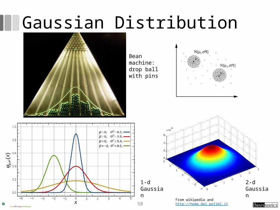
Gaussian Distribution

50From wikipedia and http://home.dei.polimi.it

Bean machine: drop ball with pins

1-d Gaussian

2-d Gaussian

A Probabilistic Hierarchical Clustering Algorithm• For a set of objects partitioned into m clusters C1, . . . ,Cm, the quality can

be measured by,

where P() is the maximum likelihood

• If we merge two clusters Cj1 and Cj2 into a cluster Cj1 C∪ j2, then, the change in quality of the overall clustering is

• Distance between clusters C1 and C2:

51

5.4 Density-Based Methods

52

Density-Based Clustering Methods• Clustering based on density (local cluster criterion), such as

density-connected points• Major features:

• Discover clusters of arbitrary shape• Handle noise• One scan• Need density parameters as termination condition

• Several interesting studies:• DBSCAN: Ester, et al. (KDD’96)• OPTICS: Ankerst, et al (SIGMOD’99).• DENCLUE: Hinneburg & D. Keim (KDD’98)• CLIQUE: Agrawal, et al. (SIGMOD’98) (more grid-based)

53

Density-Based Clustering: Basic Concepts• Two parameters:

• Eps: Maximum radius of the neighbourhood

• MinPts: Minimum number of points in an Eps-neighbourhood of that point

• NEps(q): {p belongs to D | dist(p,q) ≤ Eps}

• Directly density-reachable: A point p is directly density-reachable from a point q w.r.t. Eps, MinPts if

• p belongs to NEps(q)

• core point condition:

|NEps (q)| ≥ MinPts

54

MinPts = 5

Eps = 1 cm

p

q

Density-Reachable and Density-Connected• Density-reachable:

• A point p is density-reachable from a point q w.r.t. Eps, MinPts if there is a chain of points p1, …, pn, p1 = q, pn = p such that pi+1 is directly density-reachable from pi

• Density-connected

• A point p is density-connected to a point q w.r.t. Eps, MinPts if there is a point o such that both, p and q are density-reachable from o w.r.t. Eps and MinPts

55

p

qp1

p q

o

DBSCAN: Density-Based Spatial Clustering of Applications with Noise

• Relies on a density-based notion of cluster: A cluster is defined as a maximal set of density-connected points

• Discovers clusters of arbitrary shape in spatial databases with noise

56

Core

Border

Outlier

Eps = 1cm

MinPts = 5

DBSCAN: The Algorithm

1. Arbitrary select a point p

2. Retrieve all points density-reachable from p w.r.t. Eps and MinPts

3. If p is a core point, a cluster is formed

4. If p is a border point, no points are density-reachable from p and DBSCAN visits the next point of the database

5. Continue the process until all of the points have been processed

If a spatial index is used, the computational complexity of DBSCAN is O(nlogn), where n is the number of database objects. Otherwise, the complexity is O(n2) 57

DBSCAN: Sensitive to Parameters

58

http://webdocs.cs.ualberta.ca/~yaling/Cluster/Applet/Code/Cluster.html

OPTICS: A Cluster-Ordering Method (1999)• OPTICS: Ordering Points To Identify the Clustering Structure

• Ankerst, Breunig, Kriegel, and Sander (SIGMOD’99)• Produces a special order of the database wrt its density-

based clustering structure • This cluster-ordering contains info equiv to the density-

based clusterings corresponding to a broad range of parameter settings

• Good for both automatic and interactive cluster analysis, including finding intrinsic clustering structure

• Can be represented graphically or using visualization techniques

59

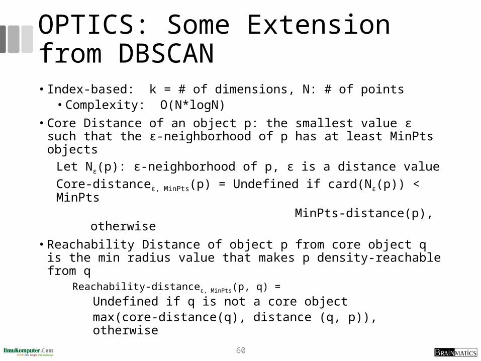
OPTICS: Some Extension from DBSCAN• Index-based: k = # of dimensions, N: # of points

• Complexity: O(N*logN)• Core Distance of an object p: the smallest value ε such that

the ε-neighborhood of p has at least MinPts objectsLet Nε(p): ε-neighborhood of p, ε is a distance valueCore-distanceε, MinPts(p) = Undefined if card(Nε(p)) < MinPts

MinPts-distance(p), otherwise• Reachability Distance of object p from core object q is the

min radius value that makes p density-reachable from qReachability-distanceε, MinPts(p, q) =

Undefined if q is not a core objectmax(core-distance(q), distance (q, p)), otherwise

60

Core Distance & Reachability Distance

61

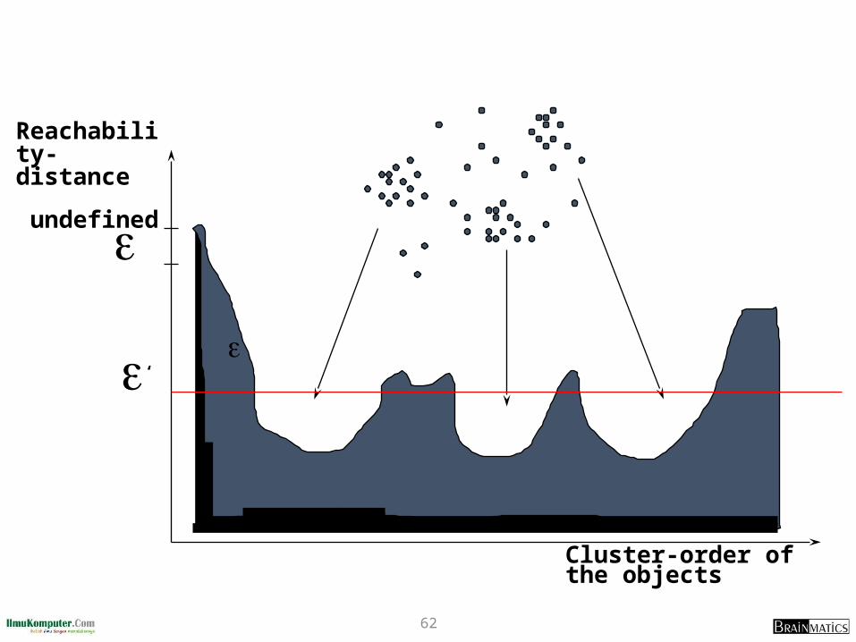
62

Reachability-distance

Cluster-order of the objects

undefined

‘

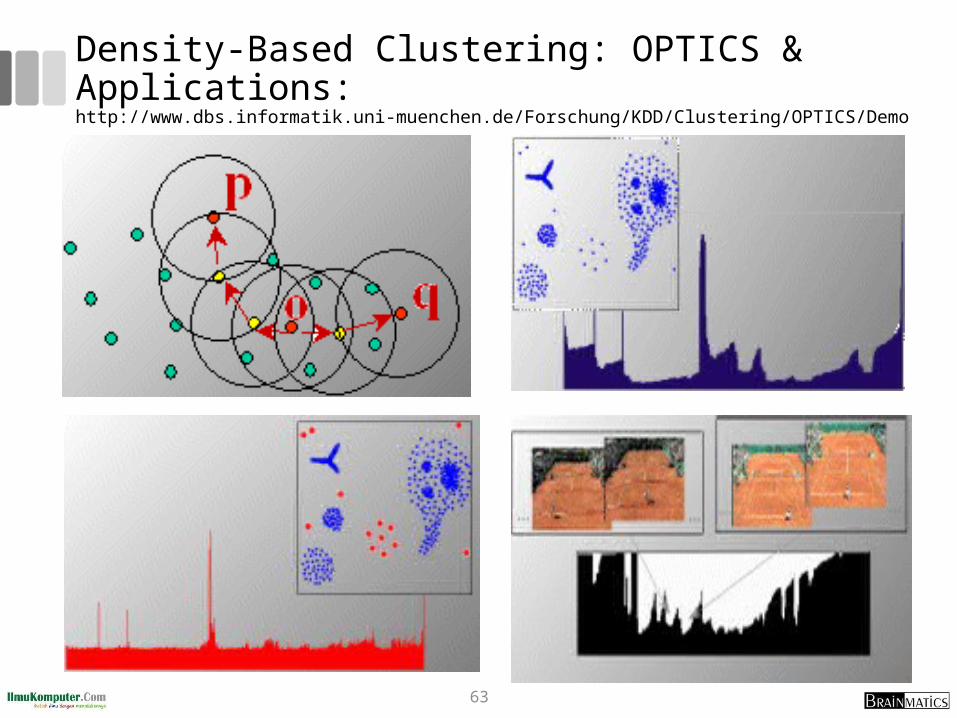
Density-Based Clustering: OPTICS & Applications:http://www.dbs.informatik.uni-muenchen.de/Forschung/KDD/Clustering/OPTICS/Demo

63

DENCLUE: Using Statistical Density Functions• DENsity-based CLUstEring by Hinneburg & Keim (KDD’98)

• Using statistical density functions:

• Major features

• Solid mathematical foundation

• Good for data sets with large amounts of noise

• Allows a compact mathematical description of arbitrarily shaped clusters in high-dimensional data sets

• Significant faster than existing algorithm (e.g., DBSCAN)

• But needs a large number of parameters

64

f x y eGaussian

d x y

( , )( , )

2

22

N

i

xxdDGaussian

i

exf1

2

),(2

2

)(

N

i

xxd

iiDGaussian

i

exxxxf1

2

),(2

2

)(),( influence of y on x

total influence on x

gradient of x in the direction of xi

Denclue: Technical Essence

• Uses grid cells but only keeps information about grid cells that do actually contain data points and manages these cells in a tree-based access structure

• Influence function: describes the impact of a data point within its neighborhood

• Overall density of the data space can be calculated as the sum of the influence function of all data points

• Clusters can be determined mathematically by identifying density attractors

• Density attractors are local maximal of the overall density function• Center defined clusters: assign to each density attractor the points

density attracted to it• Arbitrary shaped cluster: merge density attractors that are

connected through paths of high density (> threshold)65

Density Attractor

66

Center-Defined and Arbitrary

67

5.5 Grid-Based Methods

68

Grid-Based Clustering Method • Using multi-resolution grid data structure• Several interesting methods

• STING (a STatistical INformation Grid approach) by Wang, Yang and Muntz (1997)

• WaveCluster by Sheikholeslami, Chatterjee, and Zhang (VLDB’98)

• A multi-resolution clustering approach using wavelet method

• CLIQUE: Agrawal, et al. (SIGMOD’98)

• Both grid-based and subspace clustering

69

STING: A Statistical Information Grid Approach• Wang, Yang and Muntz (VLDB’97)• The spatial area is divided into rectangular cells• There are several levels of cells corresponding to

different levels of resolution

70

i-th layer

(i-1)st layer

1st layer

The STING Clustering Method• Each cell at a high level is partitioned into a number of smaller

cells in the next lower level• Statistical info of each cell is calculated and stored beforehand

and is used to answer queries• Parameters of higher level cells can be easily calculated from

parameters of lower level cell• count, mean, s, min, max • type of distribution—normal, uniform, etc.

• Use a top-down approach to answer spatial data queries• Start from a pre-selected layer—typically with a small number of

cells• For each cell in the current level compute the confidence interval

71

STING Algorithm and Its Analysis• Remove the irrelevant cells from further consideration• When finish examining the current layer, proceed to the

next lower level • Repeat this process until the bottom layer is reached• Advantages:

• Query-independent, easy to parallelize, incremental update

• O(K), where K is the number of grid cells at the lowest level

• Disadvantages:• All the cluster boundaries are either horizontal or

vertical, and no diagonal boundary is detected

72

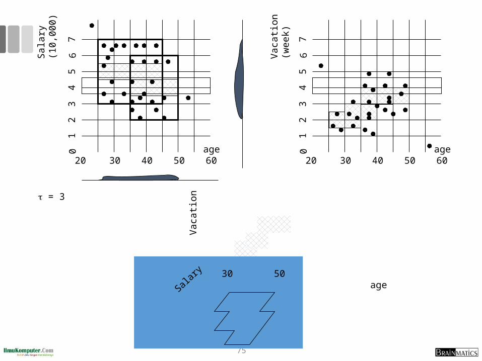
CLIQUE (Clustering In QUEst) • Agrawal, Gehrke, Gunopulos, Raghavan (SIGMOD’98)• Automatically identifying subspaces of a high

dimensional data space that allow better clustering than original space

• CLIQUE can be considered as both density-based and grid-based

• It partitions each dimension into the same number of equal length interval

• It partitions an m-dimensional data space into non-overlapping rectangular units

• A unit is dense if the fraction of total data points contained in the unit exceeds the input model parameter

• A cluster is a maximal set of connected dense units within a subspace

73

CLIQUE: The Major Steps

1. Partition the data space and find the number of points that lie inside each cell of the partition.

2. Identify the subspaces that contain clusters using the Apriori principle

3. Identify clusters1. Determine dense units in all subspaces of interests2. Determine connected dense units in all subspaces of

interests.

4. Generate minimal description for the clusters1. Determine maximal regions that cover a cluster of

connected dense units for each cluster2. Determination of minimal cover for each cluster

74

75

Sala

ry

(10,

000)

20 30 40 50 60age

54

31

26

70

20 30 40 50 60age

54

31

26

70

Vaca

tion(

wee

k)age

Vaca

tion

Salary 30 50

= 3

Strength and Weakness of CLIQUE• Strength

• automatically finds subspaces of the highest dimensionality such that high density clusters exist in those subspaces

• insensitive to the order of records in input and does not presume some canonical data distribution

• scales linearly with the size of input and has good scalability as the number of dimensions in the data increases

• Weakness• The accuracy of the clustering result may be degraded at

the expense of simplicity of the method

76

5.6 Evaluation of Clustering

77

Assessing Clustering Tendency• Assess if non-random structure exists in the data by

measuring the probability that the data is generated by a uniform data distribution

• Test spatial randomness by statistic test: Hopkins Static• Given a dataset D regarded as a sample of a random variable o,

determine how far away o is from being uniformly distributed in the data space

• Sample n points, p1, …, pn, uniformly from D. For each pi, find its nearest neighbor in D: xi = min{dist (pi, v)} where v in D

• Sample n points, q1, …, qn, uniformly from D. For each qi, find its nearest neighbor in D – {qi}: yi = min{dist (qi, v)} where v in D and v ≠ qi

• Calculate the Hopkins Statistic:

• If D is uniformly distributed, ∑ xi and ∑ yi will be close to each other and H is close to 0.5. If D is clustered, H is close to 1

78

Determine the Number of Clusters• Empirical method

• # of clusters ≈√n/2 for a dataset of n points

• Elbow method• Use the turning point in the curve of sum of within cluster variance

w.r.t the # of clusters

• Cross validation method• Divide a given data set into m parts• Use m – 1 parts to obtain a clustering model• Use the remaining part to test the quality of the clustering

• E.g., For each point in the test set, find the closest centroid, and use the sum of squared distance between all points in the test set and the closest centroids to measure how well the model fits the test set

• For any k > 0, repeat it m times, compare the overall quality measure w.r.t. different k’s, and find # of clusters that fits the data the best

79

Measuring Clustering Quality• Two methods: extrinsic vs. intrinsic

• Extrinsic: supervised, i.e., the ground truth is available

• Compare a clustering against the ground truth using certain clustering quality measure

• Ex. BCubed precision and recall metrics

• Intrinsic: unsupervised, i.e., the ground truth is unavailable

• Evaluate the goodness of a clustering by considering how well the clusters are separated, and how compact the clusters are

• Ex. Silhouette coefficient

80

Measuring Clustering Quality: Extrinsic Methods • Clustering quality measure: Q(C, Cg), for a clustering C given

the ground truth Cg. • Q is good if it satisfies the following 4 essential criteria

• Cluster homogeneity: the purer, the better• Cluster completeness: should assign objects belong to

the same category in the ground truth to the same cluster

• Rag bag: putting a heterogeneous object into a pure cluster should be penalized more than putting it into a rag bag (i.e., “miscellaneous” or “other” category)

• Small cluster preservation: splitting a small category into pieces is more harmful than splitting a large category into pieces

81

Rangkuman• Cluster analysis groups objects based on their similarity and has wide

applications

• Measure of similarity can be computed for various types of data

• Clustering algorithms can be categorized into partitioning methods, hierarchical methods, density-based methods, grid-based methods, and model-based methods

• K-means and K-medoids algorithms are popular partitioning-based clustering algorithms

• Birch and Chameleon are interesting hierarchical clustering algorithms, and there are also probabilistic hierarchical clustering algorithms

• DBSCAN, OPTICS, and DENCLU are interesting density-based algorithms

• STING and CLIQUE are grid-based methods, where CLIQUE is also a subspace clustering algorithm

• Quality of clustering results can be evaluated in various ways 82

Referensi1. Jiawei Han and Micheline Kamber, Data Mining: Concepts and Techniques

Third Edition, Elsevier, 20122. Ian H. Witten, Frank Eibe, Mark A. Hall, Data mining: Practical Machine

Learning Tools and Techniques 3rd Edition, Elsevier, 20113. Markus Hofmann and Ralf Klinkenberg, RapidMiner: Data Mining Use Cases

and Business Analytics Applications, CRC Press Taylor & Francis Group, 20144. Daniel T. Larose, Discovering Knowledge in Data: an Introduction to Data

Mining, John Wiley & Sons, 20055. Ethem Alpaydin, Introduction to Machine Learning, 3rd ed., MIT Press, 20146. Florin Gorunescu, Data Mining: Concepts, Models and Techniques, Springer,

2011 7. Oded Maimon and Lior Rokach, Data Mining and Knowledge Discovery

Handbook Second Edition, Springer, 20108. Warren Liao and Evangelos Triantaphyllou (eds.), Recent Advances in Data

Mining of Enterprise Data: Algorithms and Applications, World Scientific, 2007

83