Data Mining: 3. Persiapan Data Romi Satria Wahono [email protected] WA/SMS: +6281586220090...

Data Mining:3. Persiapan Data

Romi Satria [email protected]

http://romisatriawahono.net/dmWA/SMS: +6281586220090

1

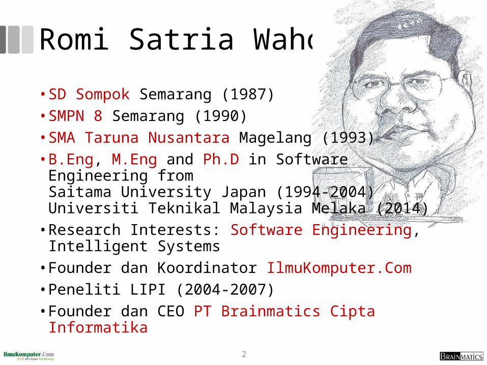
Romi Satria Wahono

• SD Sompok Semarang (1987)• SMPN 8 Semarang (1990)• SMA Taruna Nusantara Magelang (1993)• B.Eng, M.Eng and Ph.D in Software Engineering from

Saitama University Japan (1994-2004)Universiti Teknikal Malaysia Melaka (2014)

• Research Interests: Software Engineering,Intelligent Systems

• Founder dan Koordinator IlmuKomputer.Com• Peneliti LIPI (2004-2007)• Founder dan CEO PT Brainmatics Cipta Informatika

2

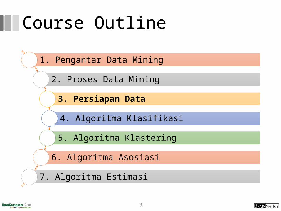
Course Outline

1. Pengantar Data Mining

2. Proses Data Mining

3. Persiapan Data

4. Algoritma Klasifikasi

5. Algoritma Klastering

6. Algoritma Asosiasi

7. Algoritma Estimasi

3

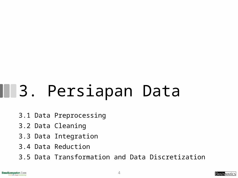
3. Persiapan Data3.1 Data Preprocessing

3.2 Data Cleaning

3.3 Data Integration

3.4 Data Reduction

3.5 Data Transformation and Data Discretization

4

3.1 Data Preprocessing

5

CRISP-DM

6

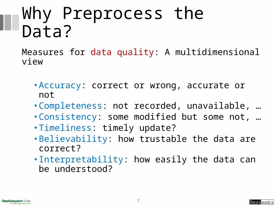
Why Preprocess the Data?

Measures for data quality: A multidimensional view

• Accuracy: correct or wrong, accurate or not• Completeness: not recorded, unavailable, …• Consistency: some modified but some not, …• Timeliness: timely update? • Believability: how trustable the data are correct?• Interpretability: how easily the data can be

understood?

7

Major Tasks in Data Preprocessing1. Data cleaning

• Fill in missing values• Smooth noisy data• Identify or remove outliers• Resolve inconsistencies

2. Data integration• Integration of multiple databases or files

3. Data reduction• Dimensionality reduction• Numerosity reduction• Data compression

4. Data transformation and data discretization• Normalization • Concept hierarchy generation

8

3.2 Data Cleaning

9

Data CleaningData in the Real World Is Dirty: Lots of potentially incorrect data, e.g., instrument faulty, human or computer error, transmission error

• Incomplete: lacking attribute values, lacking certain attributes of interest, or containing only aggregate data

• e.g., Occupation=“ ” (missing data)

• Noisy: containing noise, errors, or outliers• e.g., Salary=“−10” (an error)

• Inconsistent: containing discrepancies in codes or names• e.g., Age=“42”, Birthday=“03/07/2010”• Was rating “1, 2, 3”, now rating “A, B, C”

• Discrepancy between duplicate records• Intentional (e.g., disguised missing data)• Jan. 1 as everyone’s birthday?10

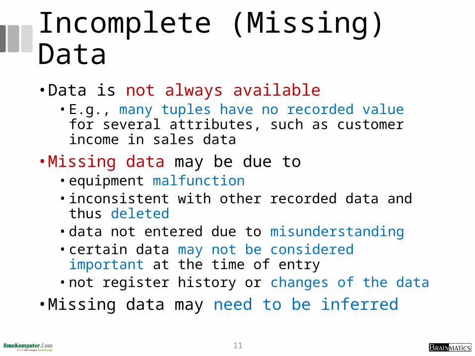
Incomplete (Missing) Data

• Data is not always available• E.g., many tuples have no recorded value for several

attributes, such as customer income in sales data

• Missing data may be due to • equipment malfunction• inconsistent with other recorded data and thus deleted• data not entered due to misunderstanding• certain data may not be considered important at the

time of entry• not register history or changes of the data

• Missing data may need to be inferred

11

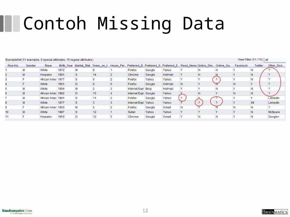
Contoh Missing Data

12

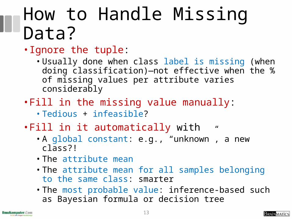
How to Handle Missing Data?• Ignore the tuple:

• Usually done when class label is missing (when doing classification)—not effective when the % of missing values per attribute varies considerably

• Fill in the missing value manually:• Tedious + infeasible?

• Fill in it automatically with• A global constant: e.g., “unknown”, a new class?! • The attribute mean• The attribute mean for all samples belonging to the same

class: smarter• The most probable value: inference-based such as

Bayesian formula or decision tree13

Latihan

• Lakukan eksperimen mengikuti buku Matthew North, Data Mining for the Masses, 2012, Chapter 3 Data Preparation, pp. 30-46 (Handling Missing Data)

• Analisis metode preprocessing apa saja yang digunakan dan mengapa perlu dilakukan pada dataset tersebut

14

Missing Value Detection

15

Noisy Data

• Noise: random error or variance in a measured variable

• Incorrect attribute values may be due to• Faulty data collection instruments• Data entry problems• Data transmission problems• Technology limitation• Inconsistency in naming convention

• Other data problems which require data cleaning• Duplicate records• Incomplete data• Inconsistent data

16

How to Handle Noisy Data?

• Binning• First sort data and partition into (equal-frequency) bins• Then one can smooth by bin means, smooth by bin

median, smooth by bin boundaries, etc.

• Regression• Smooth by fitting the data into regression functions

• Clustering• Detect and remove outliers

• Combined computer and human inspection• Detect suspicious values and check by human (e.g., deal

with possible outliers)

17

Data Cleaning as a Process• Data discrepancy detection

• Use metadata (e.g., domain, range, dependency, distribution)• Check field overloading • Check uniqueness rule, consecutive rule and null rule• Use commercial tools

• Data scrubbing: use simple domain knowledge (e.g., postal code, spell-check) to detect errors and make corrections

• Data auditing: by analyzing data to discover rules and relationship to detect violators (e.g., correlation and clustering to find outliers)

• Data migration and integration• Data migration tools: allow transformations to be specified• ETL (Extraction/Transformation/Loading) tools: allow users to

specify transformations through a graphical user interface

• Integration of the two processes• Iterative and interactive (e.g., Potter’s Wheels)

18

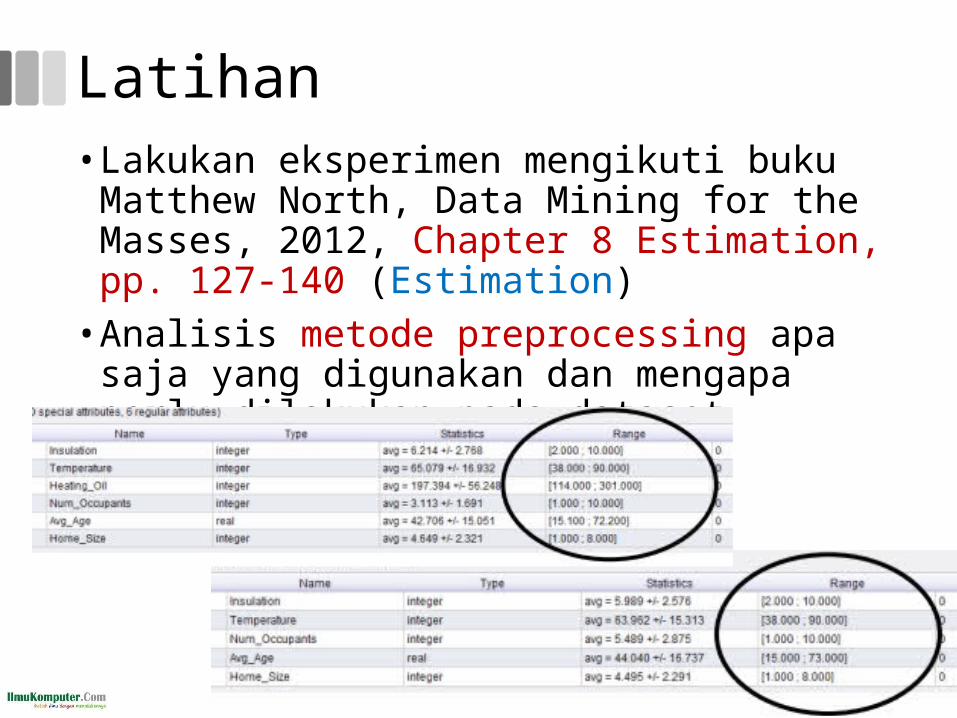
Latihan• Lakukan eksperimen mengikuti buku Matthew

North, Data Mining for the Masses, 2012, Chapter 8 Estimation, pp. 127-140 (Estimation)


19

Latihan

• Lakukan eksperimen mengikuti buku Matthew North, Data Mining for the Masses, 2012, Chapter 3 Data Preparation, pp. 50-52 (Handling Inconsistence Data)


20

3.3 Data Integration

21

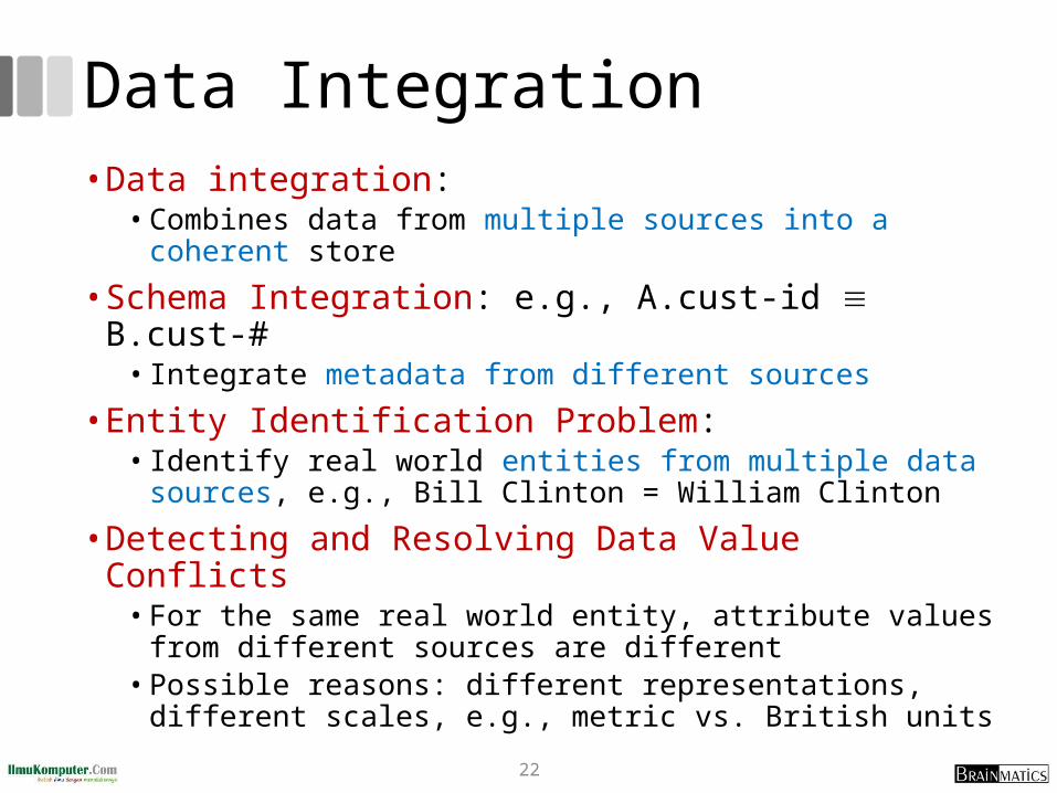
Data Integration• Data integration:

• Combines data from multiple sources into a coherent store

• Schema Integration: e.g., A.cust-id B.cust-#• Integrate metadata from different sources

• Entity Identification Problem: • Identify real world entities from multiple data sources,

e.g., Bill Clinton = William Clinton

• Detecting and Resolving Data Value Conflicts• For the same real world entity, attribute values from

different sources are different• Possible reasons: different representations, different

scales, e.g., metric vs. British units22

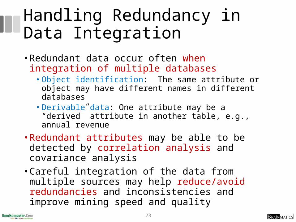
Handling Redundancy in Data Integration• Redundant data occur often when integration of

multiple databases• Object identification: The same attribute or object may

have different names in different databases• Derivable data: One attribute may be a “derived”

attribute in another table, e.g., annual revenue

• Redundant attributes may be able to be detected by correlation analysis and covariance analysis

• Careful integration of the data from multiple sources may help reduce/avoid redundancies and inconsistencies and improve mining speed and quality

23

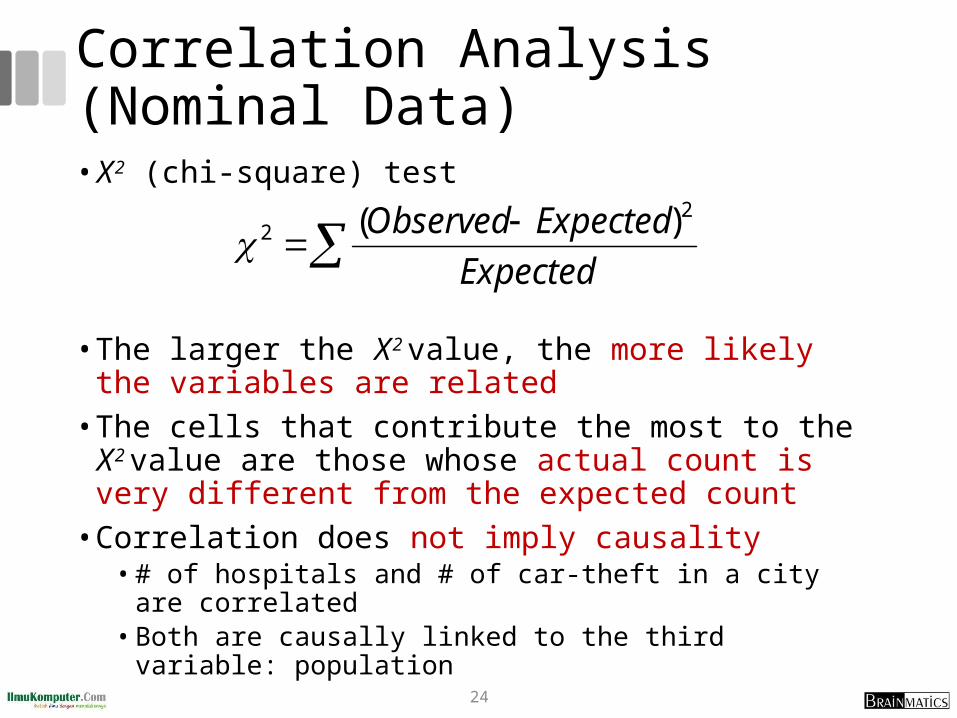
Correlation Analysis (Nominal Data)• Χ2 (chi-square) test

• The larger the Χ2 value, the more likely the variables are related

• The cells that contribute the most to the Χ2 value are those whose actual count is very different from the expected count

• Correlation does not imply causality• # of hospitals and # of car-theft in a city are correlated• Both are causally linked to the third variable: population

Expected

ExpectedObserved 22 )(

24

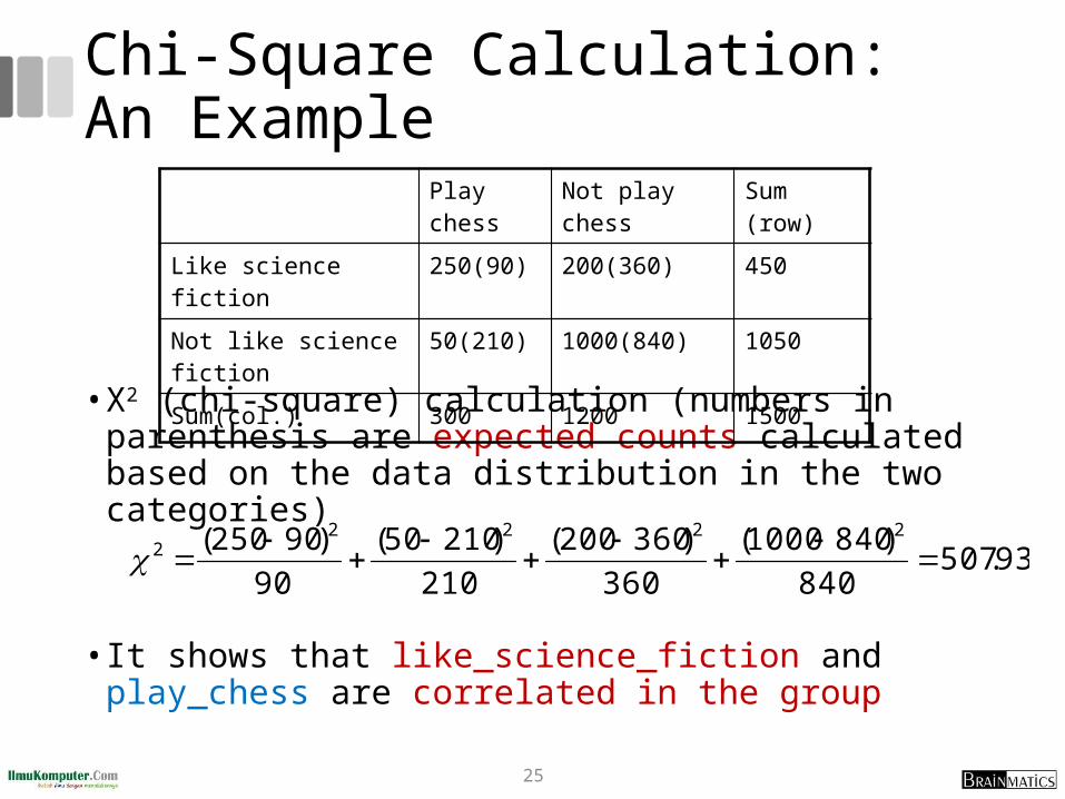
Chi-Square Calculation: An Example

• Χ2 (chi-square) calculation (numbers in parenthesis are expected counts calculated based on the data distribution in the two categories)

• It shows that like_science_fiction and play_chess are correlated in the group

Play chess

Not play chess

Sum (row)

Like science fiction 250(90) 200(360) 450

Not like science fiction

50(210) 1000(840) 1050

Sum(col.) 300 1200 1500

93.507840

)8401000(

360

)360200(

210

)21050(

90

)90250( 22222

25

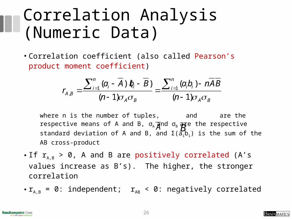
Correlation Analysis (Numeric Data)• Correlation coefficient (also called Pearson’s product moment

coefficient)

where n is the number of tuples, and are the respective means of A and B, σA and σB are the respective standard deviation of A and B, and Σ(aibi) is the sum of the AB cross-product

• If rA,B > 0, A and B are positively correlated (A’s values increase as B’s). The higher, the stronger correlation

• rA,B = 0: independent; rAB < 0: negatively correlated

BA

n

i ii

BA

n

i iiBA n

BAnba

n

BbAar

)1(

)(

)1(

))((11

,

A B

26

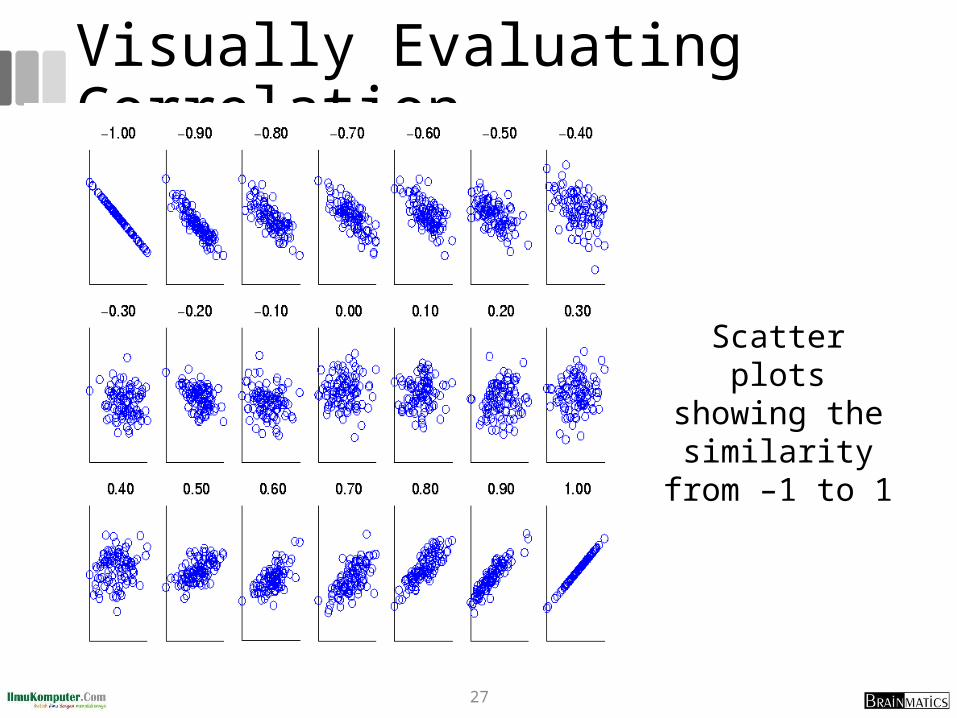
Visually Evaluating Correlation

Scatter plots showing the

similarityfrom –1 to 1

27

Correlation

• Correlation measures the linear relationship between objects

• To compute correlation, we standardize data objects, A and B, and then take their dot product

)(/))((' AstdAmeanaa kk

)(/))((' BstdBmeanbb kk

''),( BABAncorrelatio

28

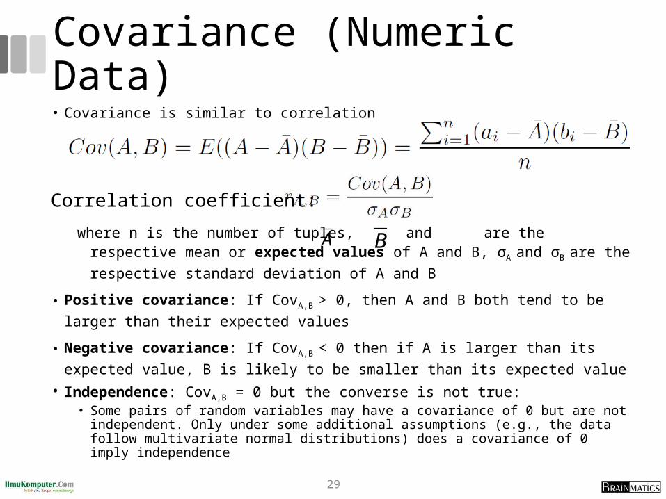
Covariance (Numeric Data)• Covariance is similar to correlation

where n is the number of tuples, and are the respective mean or expected values of A and B, σA and σB are the respective standard deviation of A and B

• Positive covariance: If CovA,B > 0, then A and B both tend to be larger than their expected values

• Negative covariance: If CovA,B < 0 then if A is larger than its expected value, B is likely to be smaller than its expected value

• Independence: CovA,B = 0 but the converse is not true:• Some pairs of random variables may have a covariance of 0 but are not independent.

Only under some additional assumptions (e.g., the data follow multivariate normal distributions) does a covariance of 0 imply independence

A B

Correlation coefficient:

29

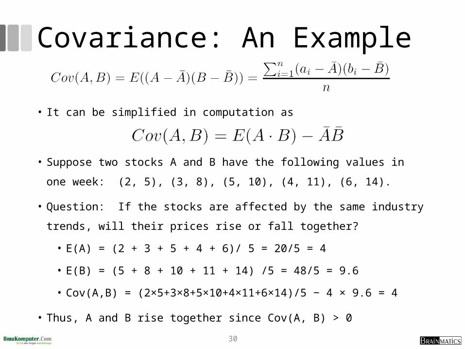
Covariance: An Example

• It can be simplified in computation as

• Suppose two stocks A and B have the following values in one week: (2, 5), (3, 8),

(5, 10), (4, 11), (6, 14).

• Question: If the stocks are affected by the same industry trends, will their prices

rise or fall together?

• E(A) = (2 + 3 + 5 + 4 + 6)/ 5 = 20/5 = 4

• E(B) = (5 + 8 + 10 + 11 + 14) /5 = 48/5 = 9.6

• Cov(A,B) = (2×5+3×8+5×10+4×11+6×14)/5 − 4 × 9.6 = 4

• Thus, A and B rise together since Cov(A, B) > 030

3.4 Data Reduction

31

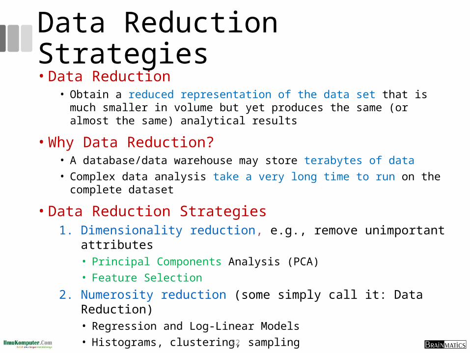
Data Reduction Strategies• Data Reduction

• Obtain a reduced representation of the data set that is much smaller in volume but yet produces the same (or almost the same) analytical results

• Why Data Reduction?• A database/data warehouse may store terabytes of data• Complex data analysis take a very long time to run on the complete dataset

• Data Reduction Strategies1. Dimensionality reduction, e.g., remove unimportant attributes

• Principal Components Analysis (PCA)• Feature Selection

2. Numerosity reduction (some simply call it: Data Reduction)• Regression and Log-Linear Models• Histograms, clustering, sampling

32

1. Dimensionality Reduction

• Curse of dimensionality• When dimensionality increases, data becomes increasingly sparse• Density and distance between points, which is critical to

clustering, outlier analysis, becomes less meaningful• The possible combinations of subspaces will grow exponentially

• Dimensionality reduction• Avoid the curse of dimensionality• Help eliminate irrelevant features and reduce noise• Reduce time and space required in data mining• Allow easier visualization

• Dimensionality reduction techniques• Wavelet transforms• Principal Component Analysis• Supervised and nonlinear techniques (e.g., feature selection)

33

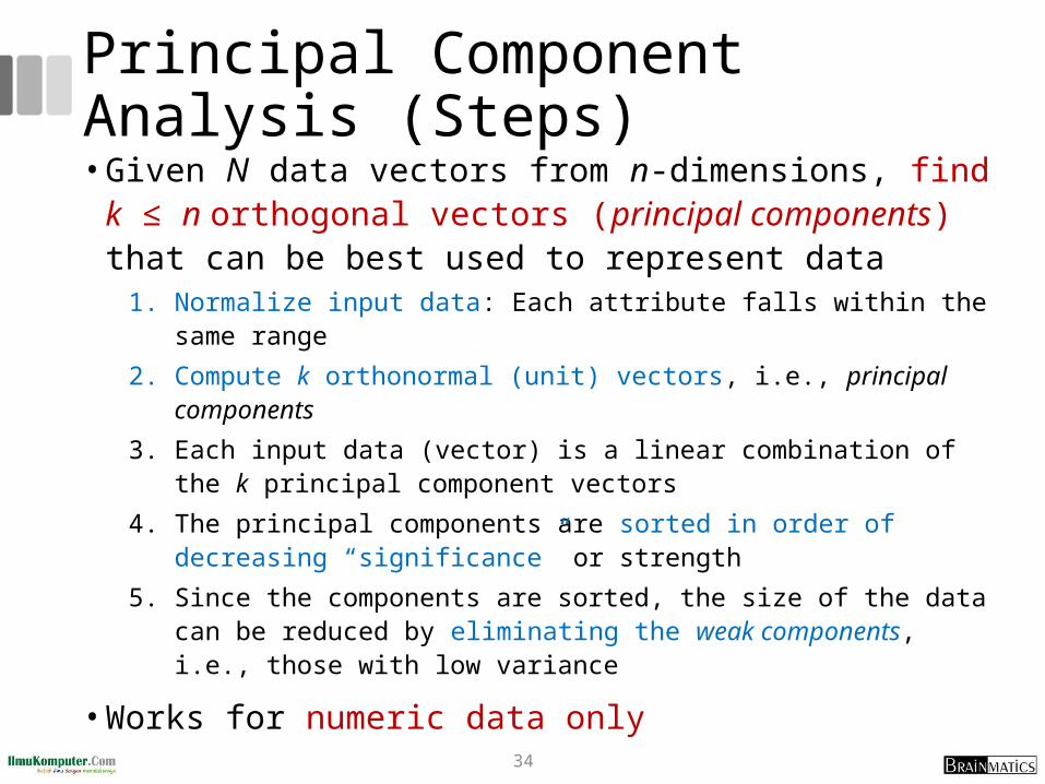
Principal Component Analysis (Steps)• Given N data vectors from n-dimensions, find k ≤ n

orthogonal vectors (principal components) that can be best used to represent data

1. Normalize input data: Each attribute falls within the same range

2. Compute k orthonormal (unit) vectors, i.e., principal components

3. Each input data (vector) is a linear combination of the k principal component vectors

4. The principal components are sorted in order of decreasing “significance” or strength

5. Since the components are sorted, the size of the data can be reduced by eliminating the weak components, i.e., those with low variance

• Works for numeric data only34

Latihan

• Lakukan eksperimen mengikuti buku Markus Hofmann (Rapid Miner - Data Mining Use Case) Chapter 4 (k-Nearest Neighbor Classification II) pp. 45-51(Dataset: glass.data)


35

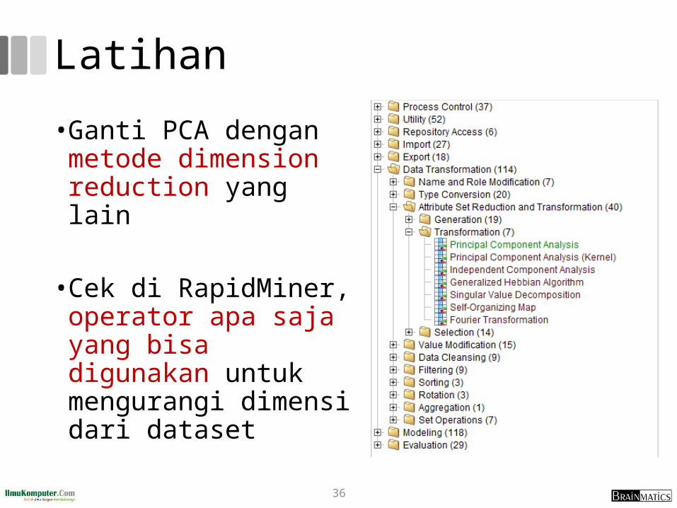
Latihan

• Ganti PCA dengan metode dimension reduction yang lain

• Cek di RapidMiner, operator apa saja yang bisa digunakan untuk mengurangi dimensi dari dataset

36

Feature/Attribute Selection

• Another way to reduce dimensionality of data

• Redundant attributes • Duplicate much or all of the information contained in

one or more other attributes• E.g., purchase price of a product and the amount of

sales tax paid

• Irrelevant attributes• Contain no information that is useful for the data mining

task at hand• E.g., students' ID is often irrelevant to the task of

predicting students' GPA37

Feature Selection ApproachA number of proposed approaches for feature selection can broadly be categorized into the following three classifications: wrapper, filter, and hybrid (Liu & Tu, 2004)

1. In the filter approach, statistical analysis of the feature set is required, without utilizing any learning model (Dash & Liu, 1997)

2. In the wrapper approach, a predetermined learning model is assumed, wherein features are selected that justify the learning performance of the particular learning model (Guyon & Elisseeff, 2003)

3. The hybrid approach attempts to utilize the complementary strengths of the wrapper and filter approaches (Huang, Cai, & Xu, 2007)

38

Wrapper Approach vs Filter Approach

39

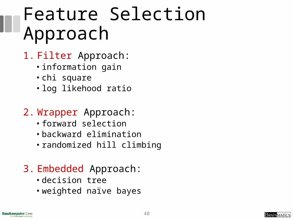
Feature Selection Approach1. Filter Approach:

• information gain• chi square• log likehood ratio

2. Wrapper Approach:• forward selection• backward elimination• randomized hill climbing

3. Embedded Approach:• decision tree• weighted naïve bayes

40

Latihan

• Lakukan eksperimen mengikuti buku Markus Hofmann (Rapid Miner - Data Mining Use Case) Chapter 4 (k-Nearest Neighbor Classification II)

• Ganti PCA dengan metode feature selection yang lain

• Cek di RapidMiner, operator apa saja yang bisa digunakan untuk mengurangi atau membobot atribute dari dataset

41

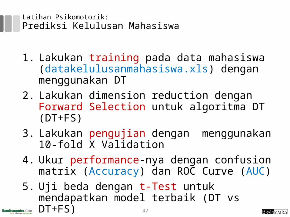
Latihan Psikomotorik:Prediksi Kelulusan Mahasiswa

1. Lakukan training pada data mahasiswa (datakelulusanmahasiswa.xls) dengan menggunakan DT

2. Lakukan dimension reduction dengan Forward Selection untuk algoritma DT (DT+FS)

3. Lakukan pengujian dengan menggunakan 10-fold X Validation

4. Ukur performance-nya dengan confusion matrix (Accuracy) dan ROC Curve (AUC)

5. Uji beda dengan t-Test untuk mendapatkan model terbaik (DT vs DT+FS)

42

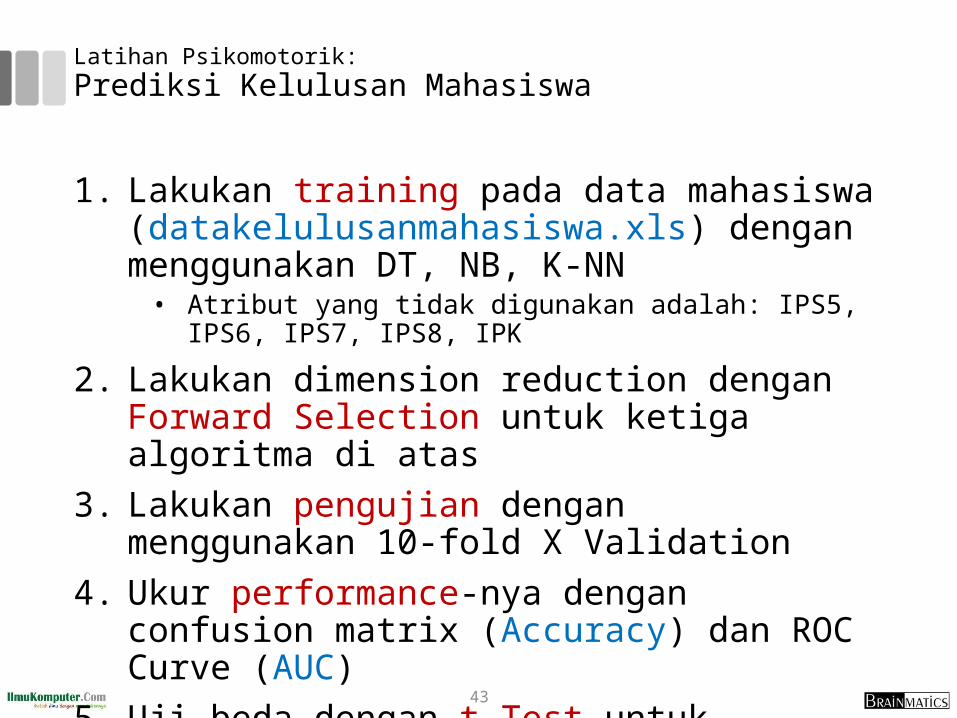
Latihan Psikomotorik:Prediksi Kelulusan Mahasiswa

1. Lakukan training pada data mahasiswa (datakelulusanmahasiswa.xls) dengan menggunakan DT, NB, K-NN

• Atribut yang tidak digunakan adalah: IPS5, IPS6, IPS7, IPS8, IPK

2. Lakukan dimension reduction dengan Forward Selection untuk ketiga algoritma di atas

3. Lakukan pengujian dengan menggunakan 10-fold X Validation

4. Ukur performance-nya dengan confusion matrix (Accuracy) dan ROC Curve (AUC)

5. Uji beda dengan t-Test untuk mendapatkan model terbaik

43

Prediksi Kelulusan Mahasiswa: Result• Komparasi Accuracy dan AUC

• Uji Beda (t-Test)

• Urutan model terbaik:44

DT NB K-NN DT+FS NB+FS K-NN+FS

Accuracy

AUC

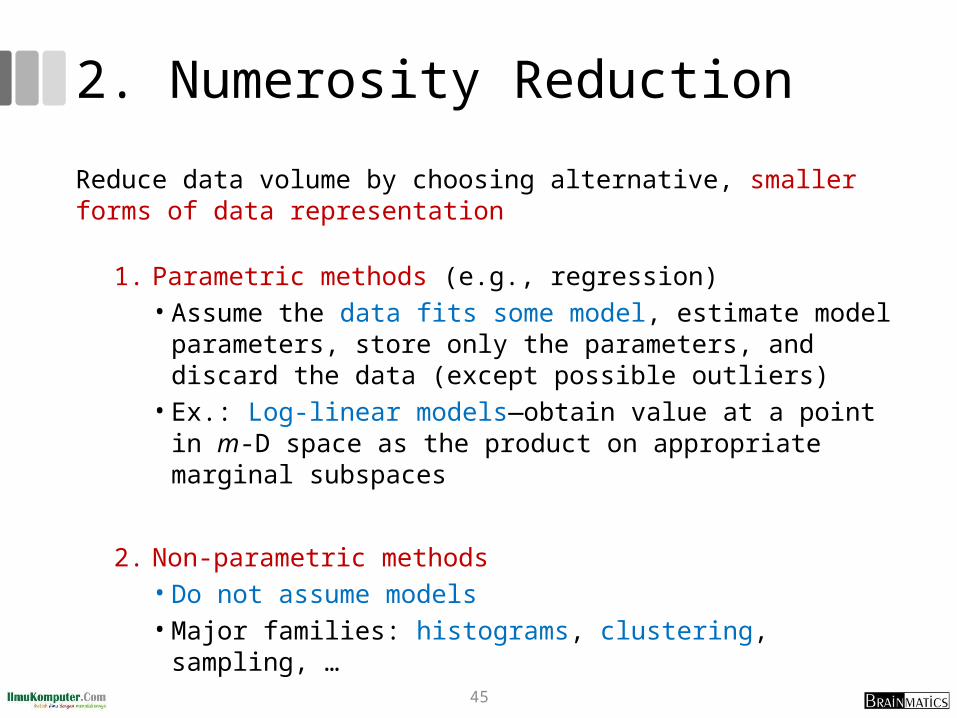
2. Numerosity Reduction

Reduce data volume by choosing alternative, smaller forms of data representation

1. Parametric methods (e.g., regression)• Assume the data fits some model, estimate model

parameters, store only the parameters, and discard the data (except possible outliers)

• Ex.: Log-linear models—obtain value at a point in m-D space as the product on appropriate marginal subspaces

2. Non-parametric methods • Do not assume models• Major families: histograms, clustering, sampling, …

45

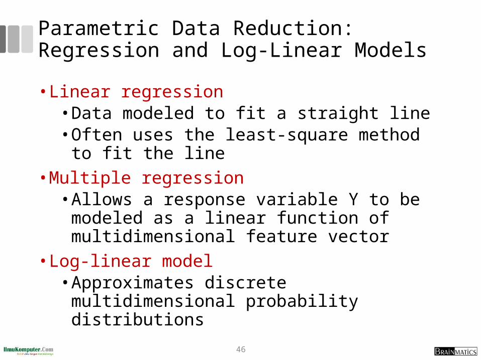
Parametric Data Reduction: Regression and Log-Linear Models

• Linear regression• Data modeled to fit a straight line• Often uses the least-square method to fit the

line• Multiple regression

• Allows a response variable Y to be modeled as a linear function of multidimensional feature vector

• Log-linear model• Approximates discrete multidimensional

probability distributions46

Regression Analysis• Regression analysis: A collective name for

techniques for the modeling and analysis of numerical data consisting of values of a dependent variable (also called response variable or measurement) and of one or more independent variables (aka. explanatory variables or predictors)

• The parameters are estimated so as to give a "best fit" of the data

• Most commonly the best fit is evaluated by using the least squares method, but other criteria have also been used

• Used for prediction (including forecasting of time-series data), inference, hypothesis testing, and modeling of causal relationships

x

y = x + 1

X1

Y1

Y1’

47

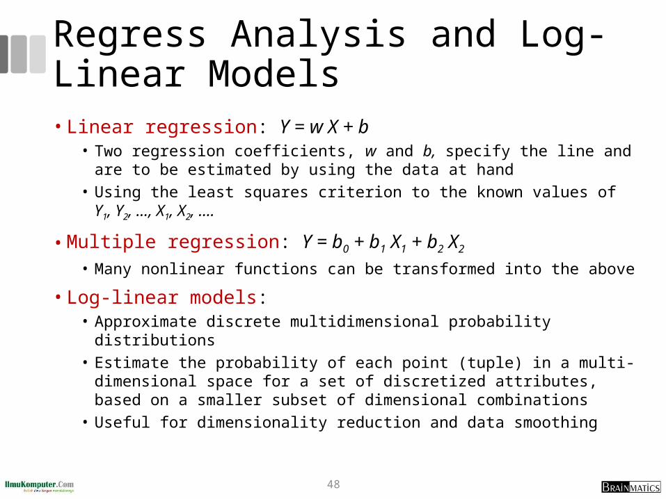
Regress Analysis and Log-Linear Models• Linear regression: Y = w X + b

• Two regression coefficients, w and b, specify the line and are to be estimated by using the data at hand

• Using the least squares criterion to the known values of Y1, Y2, …, X1, X2, ….

• Multiple regression: Y = b0 + b1 X1 + b2 X2

• Many nonlinear functions can be transformed into the above

• Log-linear models:• Approximate discrete multidimensional probability distributions• Estimate the probability of each point (tuple) in a multi-dimensional

space for a set of discretized attributes, based on a smaller subset of dimensional combinations

• Useful for dimensionality reduction and data smoothing48

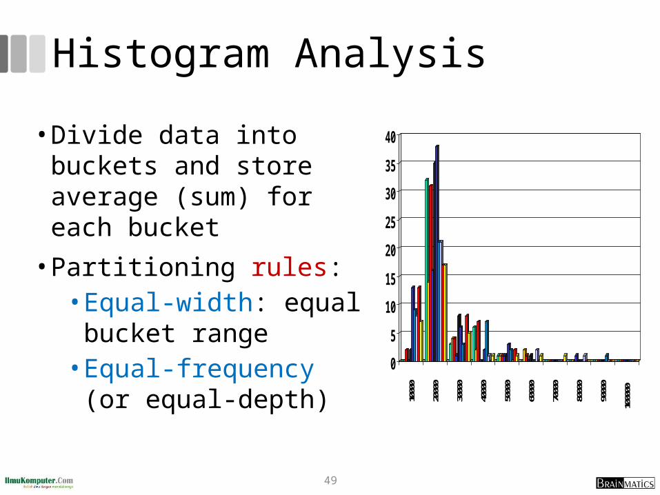
Histogram Analysis

• Divide data into buckets and store average (sum) for each bucket

• Partitioning rules:• Equal-width: equal bucket

range• Equal-frequency (or equal-

depth) 0

5

10

15

20

25

30

35

40

10000

20000

30000

40000

50000

60000

70000

80000

90000

100000

49

Clustering

• Partition data set into clusters based on similarity, and store cluster representation (e.g., centroid and diameter) only

• Can be very effective if data is clustered but not if data is “smeared”

• Can have hierarchical clustering and be stored in multi-dimensional index tree structures

• There are many choices of clustering definitions and clustering algorithms

50

Sampling• Sampling: obtaining a small sample s to represent

the whole data set N• Allow a mining algorithm to run in complexity that

is potentially sub-linear to the size of the data• Key principle: Choose a representative subset of the

data• Simple random sampling may have very poor performance in the

presence of skew• Develop adaptive sampling methods, e.g., stratified sampling

• Note: Sampling may not reduce database I/Os (page at a time)

51

Types of Sampling

• Simple random sampling• There is an equal probability of selecting any particular item

• Sampling without replacement• Once an object is selected, it is removed from the

population• Sampling with replacement

• A selected object is not removed from the population• Stratified sampling

• Partition the data set, and draw samples from each partition (proportionally, i.e., approximately the same percentage of the data)

• Used in conjunction with skewed data

52

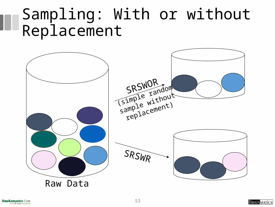
Sampling: With or without Replacement

SRSWOR

(simple random

sample without

replacement)

SRSWR

Raw Data

53

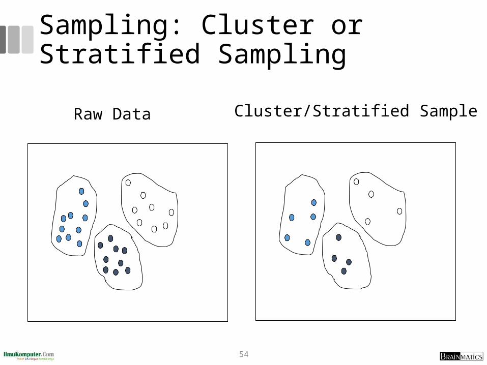
Sampling: Cluster or Stratified Sampling

Raw Data Cluster/Stratified Sample

54

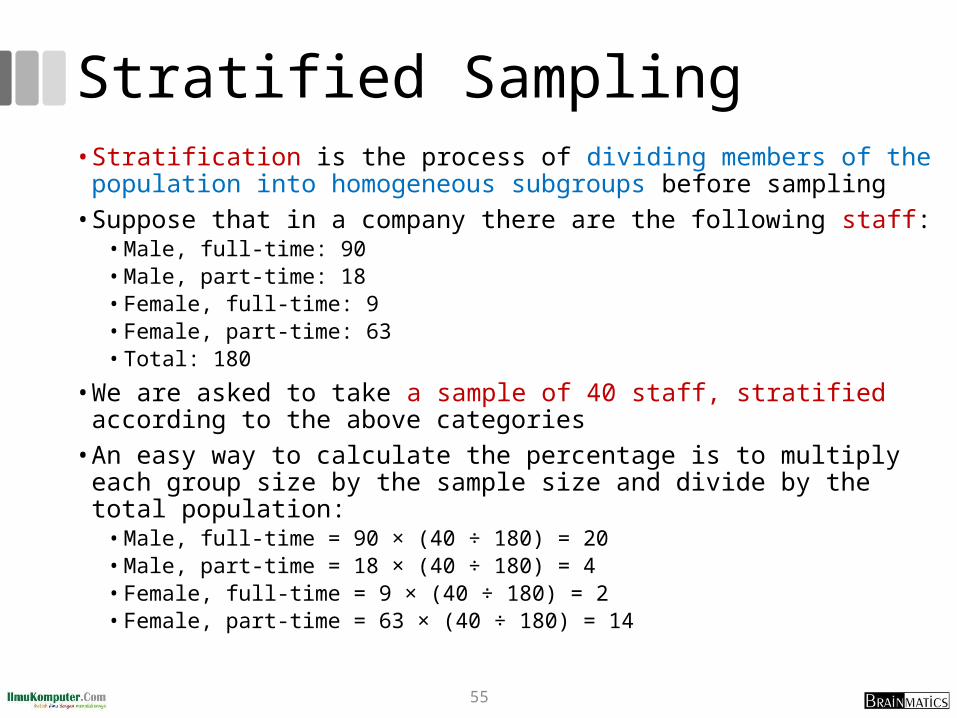
Stratified Sampling• Stratification is the process of dividing members of the population

into homogeneous subgroups before sampling • Suppose that in a company there are the following staff:

• Male, full-time: 90• Male, part-time: 18• Female, full-time: 9• Female, part-time: 63• Total: 180

• We are asked to take a sample of 40 staff, stratified according to the above categories

• An easy way to calculate the percentage is to multiply each group size by the sample size and divide by the total population:

• Male, full-time = 90 × (40 ÷ 180) = 20• Male, part-time = 18 × (40 ÷ 180) = 4• Female, full-time = 9 × (40 ÷ 180) = 2• Female, part-time = 63 × (40 ÷ 180) = 1455

Latihan

• Lakukan eksperimen mengikuti buku Matthew North, Data Mining for the Masses, 2012, Chapter 3 Data Preparation, pp. 46-50 (Data Reduction)


56

3.5 Data Transformation and Data Discretization

57

Data Transformation• A function that maps the entire set of values of a given attribute to

a new set of replacement values• Each old value can be identified with one of the new values

• Methods:• Smoothing: Remove noise from data

• Attribute/feature construction

• New attributes constructed from the given ones

• Aggregation: Summarization, data cube construction

• Normalization: Scaled to fall within a smaller, specified range

• min-max normalization

• z-score normalization

• normalization by decimal scaling

• Discretization: Concept hierarchy climbing58

Normalization• Min-max normalization: to [new_minA, new_maxA]

• Ex. Let income range $12,000 to $98,000 normalized to [0.0, 1.0]. Then $73,000 is mapped to

• Z-score normalization (μ: mean, σ: standard deviation):

• Ex. Let μ = 54,000, σ = 16,000. Then

• Normalization by decimal scaling

716.00)00.1(000,12000,98

000,12600,73

AAA

AA

A

minnewminnewmaxnewminmax

minvv _)__('

A

Avv

'

j

vv

10' Where j is the smallest integer such that Max(|ν’|) < 1

225.1000,16

000,54600,73

59

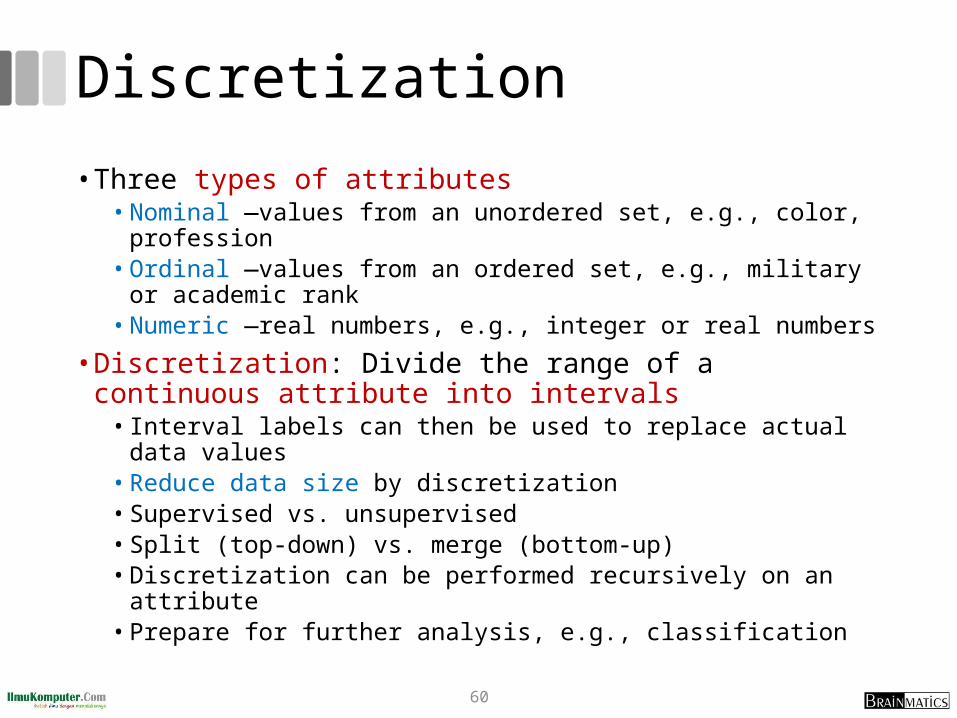
Discretization

• Three types of attributes• Nominal —values from an unordered set, e.g., color,

profession• Ordinal —values from an ordered set, e.g., military or

academic rank • Numeric —real numbers, e.g., integer or real numbers

• Discretization: Divide the range of a continuous attribute into intervals

• Interval labels can then be used to replace actual data values • Reduce data size by discretization• Supervised vs. unsupervised• Split (top-down) vs. merge (bottom-up)• Discretization can be performed recursively on an attribute• Prepare for further analysis, e.g., classification

60

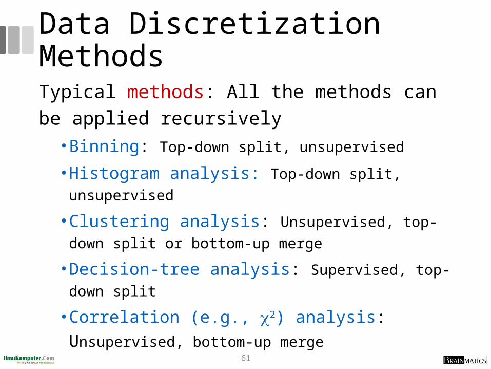
Data Discretization MethodsTypical methods: All the methods can be applied recursively

• Binning: Top-down split, unsupervised

• Histogram analysis: Top-down split, unsupervised

• Clustering analysis: Unsupervised, top-down split or bottom-up merge

• Decision-tree analysis: Supervised, top-down split

• Correlation (e.g., 2) analysis: Unsupervised, bottom-up merge

61

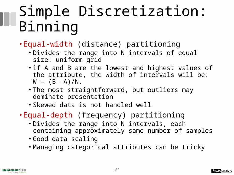
Simple Discretization: Binning• Equal-width (distance) partitioning

• Divides the range into N intervals of equal size: uniform grid• if A and B are the lowest and highest values of the attribute,

the width of intervals will be: W = (B –A)/N.• The most straightforward, but outliers may dominate

presentation• Skewed data is not handled well

• Equal-depth (frequency) partitioning• Divides the range into N intervals, each containing

approximately same number of samples• Good data scaling• Managing categorical attributes can be tricky

62

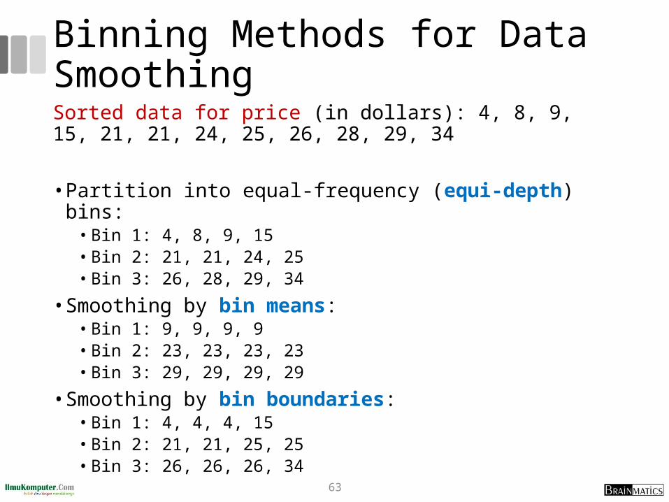
Binning Methods for Data SmoothingSorted data for price (in dollars): 4, 8, 9, 15, 21, 21, 24, 25, 26, 28, 29, 34

• Partition into equal-frequency (equi-depth) bins:• Bin 1: 4, 8, 9, 15• Bin 2: 21, 21, 24, 25• Bin 3: 26, 28, 29, 34

• Smoothing by bin means:• Bin 1: 9, 9, 9, 9• Bin 2: 23, 23, 23, 23• Bin 3: 29, 29, 29, 29

• Smoothing by bin boundaries:• Bin 1: 4, 4, 4, 15• Bin 2: 21, 21, 25, 25• Bin 3: 26, 26, 26, 34

63

Discretization Without Using Class Labels (Binning vs. Clustering)

Data Equal interval width (binning)

Equal frequency (binning) K-means clustering leads to better results

64

Discretization by Classification & Correlation Analysis• Classification (e.g., decision tree analysis)

• Supervised: Given class labels, e.g., cancerous vs. benign• Using entropy to determine split point (discretization point)• Top-down, recursive split

• Correlation analysis (e.g., Chi-merge: χ2-based discretization)

• Supervised: use class information• Bottom-up merge: find the best neighboring intervals (those

having similar distributions of classes, i.e., low χ2 values) to merge

• Merge performed recursively, until a predefined stopping condition

65

Latihan

• Lakukan eksperimen mengikuti buku Markus Hofmann (Rapid Miner - Data Mining Use Case) Chapter 5 (Naïve Bayes Classification I)


66

Rangkuman1. Data quality: accuracy, completeness, consistency,

timeliness, believability, interpretability2. Data cleaning: e.g. missing/noisy values, outliers3. Data integration from multiple sources:

• Entity identification problem• Remove redundancies• Detect inconsistencies

4. Data reduction• Dimensionality reduction• Numerosity reduction

5. Data transformation and data discretization• Normalization

67

Referensi1. Jiawei Han and Micheline Kamber, Data Mining: Concepts and Techniques

Third Edition, Elsevier, 20122. Ian H. Witten, Frank Eibe, Mark A. Hall, Data mining: Practical Machine

Learning Tools and Techniques 3rd Edition, Elsevier, 20113. Markus Hofmann and Ralf Klinkenberg, RapidMiner: Data Mining Use Cases

and Business Analytics Applications, CRC Press Taylor & Francis Group, 20144. Daniel T. Larose, Discovering Knowledge in Data: an Introduction to Data

Mining, John Wiley & Sons, 20055. Ethem Alpaydin, Introduction to Machine Learning, 3rd ed., MIT Press, 20146. Florin Gorunescu, Data Mining: Concepts, Models and Techniques, Springer,

2011 7. Oded Maimon and Lior Rokach, Data Mining and Knowledge Discovery

Handbook Second Edition, Springer, 20108. Warren Liao and Evangelos Triantaphyllou (eds.), Recent Advances in Data

Mining of Enterprise Data: Algorithms and Applications, World Scientific, 2007

68

Data Mining: 3. Persiapan Data Romi Satria Wahono [email protected] WA/SMS: +6281586220090...

Documents

Transcript of Data Mining: 3. Persiapan Data Romi Satria Wahono [email protected] WA/SMS: +6281586220090...