DAHLKE, M., JAY BREIDT, F., OPSOMER, J. and I. … · NONPARAMETRIC ENDOGENOUS POST-STRATIFICATION...
23
T E C H N I C A L R E P O R T 11004 Nonparametric endogenous post-stratification estimation DAHLKE, M., JAY BREIDT, F., OPSOMER, J. and I. VAN KEILEGOM * IAP STATISTICS NETWORK INTERUNIVERSITY ATTRACTION POLE http://www.stat.ucl.ac.be/IAP
Transcript of DAHLKE, M., JAY BREIDT, F., OPSOMER, J. and I. … · NONPARAMETRIC ENDOGENOUS POST-STRATIFICATION...

T E C H N I C A L
R E P O R T
11004
Nonparametric endogenous post-stratification estimation
DAHLKE, M., JAY BREIDT, F., OPSOMER, J. and I. VAN KEILEGOM
*
I A P S T A T I S T I C S
N E T W O R K
INTERUNIVERSITY ATTRACTION POLE
http://www.stat.ucl.ac.be/IAP

Statistica Sinica (2011): Preprint 1
NONPARAMETRIC ENDOGENOUS
POST-STRATIFICATION ESTIMATION
Mark Dahlke1, F. Jay Breidt1, Jean D. Opsomer1 and Ingrid Van Keilegom2
1Colorado State University and 2Universite catholique de Louvain
Abstract: Post-stratification is used to improve the precision of survey estimators
when categorical auxiliary information is available from external sources. In natu-
ral resource surveys, such information may be obtained from remote sensing data
classified into categories and displayed as maps. These maps may be based on clas-
sification models fitted to the sample data. Such “endogenous post-stratification”
violates the standard assumptions that observations are classified without error
into post-strata, and post-stratum population counts are known. Properties of
the endogenous post-stratification estimator (EPSE) are derived for the case of
sample-fitted nonparametric models, with particular emphasis on monotone regres-
sion models. Asymptotic properties of the nonparametric EPSE are investigated
under a superpopulation model framework. Simulation experiments illustrate the
practical effects of first fitting a nonparametric model to survey data before post-
stratifying.
Key words and phrases: Monotone regression, smoothing, survey estimation.
1. Introduction
Post-stratification is a common method for improving the precision of survey
estimators when categorical auxiliary information is available from sources ex-
ternal to the survey. In surveys of natural resources, auxiliary information may
be obtained from remote sensing data, classified into categories and displayed as
pixel-based maps. These maps may be constructed based on classification mod-
els fitted to sample data. Methods used by the US Forest Service in its Forest
Inventory and Analysis program include post-stratification (PS) of the sample
data based on categories derived from the sample data. Such “endogenous post-
stratification” violates the standard post-stratification assumptions that observa-
tions are classified without error into post-strata, and post-stratum population

NONPARAMETRIC ENDOGENOUS POST-STRATIFICATION 2
counts are known. Breidt and Opsomer (2008) derived properties of the en-
dogenous post-stratification estimator for the case of a sample-fitted generalized
linear model, from which the post-strata are constructed by dividing the range
of the model predictions into predetermined intervals. Design consistency of the
endogenous post-stratification estimator was established under general unequal-
probability sampling designs. Under a superpopulation model, consistency and
asymptotic normality of the endogenous post-stratification estimator (EPSE)
were established, showing that EPSE has the same asymptotic variance as the
traditional post-stratified estimator with fixed strata. Simulation experiments
demonstrated that the practical effect of first fitting a model to the survey data
before post-stratifying is small, even for relatively small sample sizes.
The motivation for studying endogenous post-stratification came from meth-
ods used by the U.S. Forest Service in producing estimators for the Forest Inven-
tory and Analysis (FIA; see Frayer and Furnival 1999). These methods rely on
post-stratification using classification maps derived from satellite imagery and
other ancillary information. Because the FIA data represent a source of high
quality ground-level information of forest characteristics, there is a clear desire
for being “allowed” to use them in calibrating, i.e. estimating, the classification
maps, and hence to apply EPSE in FIA. The results in Breidt and Opsomer
(2008) were considered to provide some “weak justification” for doing so (see
Czaplewski 2010), but the fact that they are restricted to parametric models
limits their applicability in the FIA context, where the methods being used are
often nonparametric in nature (e.g. Moisen and Frescino 2002).
In this paper, we extend the EPSE methodology to the nonparametric es-
timation context. We show here that the superpopulation results obtained for
EPSE by Breidt and Opsomer (2008) continue to hold in this case. We focus
on the case where the underlying model is nonparametric but monotone, which
is the most reasonable scenario in surveys since the model is used to divide the
sample into homogeneous classes. Our theoretical results are valid for a general
class of nonparametric estimators that includes kernel regression and penalized
spline regression.
In the following section we give the definitions of the estimators we propose
in this paper. The asymptotic results are given in Section 3. Section 4 examines

NONPARAMETRIC ENDOGENOUS POST-STRATIFICATION 3
some of the models and estimators satisfying the outlined conditions, and in
Section 5 we present the results of a small simulation study. The proofs of the
asymptotic results are collected in the Appendix.
2. Definition of the estimator
Consider a finite population UN = {1, . . . , i, . . . , N}. For each i ∈ UN , an
auxiliary vector xi is observed. A probability sample s of size n is drawn from UN
according to a sampling design pN(·), where pN(s) is the probability of drawing
the sample s. Assume πiN = Pr {i ∈ s} =∑
s:i∈s pN(s) > 0 for all i ∈ UN , and
define πijN = Pr {i, j ∈ s} =∑
s:i,j∈s pN(s) for all i, j ∈ UN . For compactness
of notation we will suppress the subscript N and write πi, πij in what follows.
Various study variables, generically denoted yi, are observed for i ∈ s.The targets of estimation are the finite population means of the survey vari-
ables, yN = N−1∑
UNyi. A purely design-based estimator (with all randomness
coming exclusively from the selection of s) is provided by the Horvitz-Thompson
estimator (HTE)
yπ =1N
∑i∈s
yiπi.
Post-stratification (PS) and endogenous post-stratification are methods that take
advantage of auxiliary information available for the population to improve the
efficiency of design-based estimators. Following Breidt and Opsomer (2008), we
first introduce some non-standard notation for PS that will be useful in our later
discussion of endogenous PS. Using the {xi}i∈UNand a real-valued function m(·),
a scalar index {m(xi)}i∈UNis constructed and used to partition UN into H strata
according to predetermined stratum boundaries −∞ ≤ τ0 < τ1 < · · · < τH−1 <
τH ≤ ∞. Typically, m(·) will be the true relationship between a specific study
variable zi and the auxiliary variable/vector xi. We assume the following additive
error model,
zi = m(xi) + σ(xi)εi, (2.1)
where σ2(xi) is the unknown variance function, and E(εi|xi) = 0,Var(εi|xi) = 1.
Breidt and Opsomer (2008) considered the particular case in which the index
function m(·) is parameterized by a vector, λ. We will write mλ(xi) in that case.

NONPARAMETRIC ENDOGENOUS POST-STRATIFICATION 4
For exponents ` = 0, 1, 2 and stratum indices h = 1, . . . ,H, define
ANh`(m) =1N
∑i∈UN
y`i I{τh−1<m(xi)≤τh}
and
A∗Nh`(m) =1N
∑i∈UN
y`iI{i∈s}πi
I{τh−1<m(xi)≤τh} (2.2)
where I{C} = 1 if the event C occurs, and zero otherwise. In this notation,
stratum h has population stratum proportion ANh0(m), design-weighted sample
post-stratum proportion A∗Nh0(m), and design-weighted sample post-stratum y-
mean A∗Nh1(m)/A∗Nh0(m). The traditional design-weighted PS estimator (PSE)
for the population mean yN = N−1∑
i∈UNyi is then
µ∗y(m) =H∑h=1
ANh0(m)A∗Nh1(m)A∗Nh0(m)
=∑i∈s
{H∑h=1
ANh0(m)N−1π−1
i I{τh−1<m(xi)≤τh}
A∗Nh0(m)
}yi =
∑i∈s
w∗is(m)yi, (2.3)
where the sample-dependent weights {w∗is(m)}i∈s do not depend on {yi}, and so
can be used for any study variable.
For the important special case of equal-probability designs, in which πi =
nN−1, we write
Anh`(m) =1n
∑i∈s
y`i I{τh−1<m(xi)≤τh}.
In this case, the equal-probability PSE for the population mean yN is
µy(m) =H∑h=1
ANh0(m)Anh1(m)Anh0(m)
=∑i∈s
wis(m)yi,
where the weights {wis(m)}i∈s are obtained by substituting nN−1 for πi in (2.3).
In parametric PS, the vector λ is known. In parametric endogenous PS, the
vector λ is not known and needs to be estimated from the sample {xi, zi : i ∈s} using, for example, maximum likelihood estimation or estimating equations.
Thus, mλ(xi) is estimated by mλ(xi), and the endogenous post-stratification

NONPARAMETRIC ENDOGENOUS POST-STRATIFICATION 5
estimator (EPSE) for the population mean yN is then defined as
µ∗y(mλ) =H∑h=1
ANh0(mλ)A∗Nh1(mλ)A∗Nh0(mλ)
=∑i∈s
w∗is(mλ)yi.
This parametric EPSE was studied in Breidt and Opsomer (2008). We consider
now the case where m(·) is not assumed to follow a specific parametric shape.
Again, m is typically the true regression relationship between a specific study
variable zi and an auxiliary variable/vector xi as in model (2.1).
The estimator µ∗y(m) is infeasible, because m(·) is unknown. We can estimate
m(·) from the sample {(xi, zi) : i ∈ s} by nonparametric regression, and in
this article we will explicitly consider both kernel and spline-based methods.
However, results should also apply to other nonparametric and semi-parametric
fitting methods such as regression trees, neural nets, GAMs, etc. Writing m
for the nonparametric estimator, the nonparametric endogenous post-stratified
estimator is then defined as
µ∗y(m) =H∑h=1
ANh0(m)A∗Nh1(m)A∗Nh0(m)
. (2.4)
For the important special case of equal-probability designs, in which πi =
nN−1, the equal-probability NEPSE for the population mean yN is
µy(m) =H∑h=1
ANh0(m)Anh1(m)Anh0(m)
=∑i∈s
wis(m)yi.
In order to study the properties of this estimator, it is sufficient to consider
the following simpler estimators
Aτ`(m) =1N
∑i∈UN
y`i I{m(xi)≤τ}
and
A∗τ`(m) =1N
∑i∈UN
I{i∈s}πi
y`i I{m(xi)≤τ},
for a generic boundary value τ ∈ {τ0, τ1, · · · , τH}. For equal probability designs

NONPARAMETRIC ENDOGENOUS POST-STRATIFICATION 6
we write
Anτ`(m) =1n
∑i∈s
y`i I{m(xi)≤τ}.
The form of these estimators suggests the use of tools from empirical process
theory, which we turn to in the next section.
3. Main results
3.1 Superpopulation model assumptions
Before we explicitly state the model assumptions for studying the NEPSE es-
timator, we need to introduce the concept of bracketing number of empirical
process theory (van der Vaart and Wellner 1996). For any ε > 0, any class Gof measurable functions, and any norm ‖ · ‖G defined on G, N[ ](ε,G, ‖ · ‖G) is
the bracketing number, i.e. the minimal positive integer M for which there exist
ε-brackets {[lj , uj ] : ‖lj − uj‖G ≤ ε, ‖lj‖G , ‖uj‖G < ∞, j = 1, . . . ,M} to cover G(i.e. for each g ∈ G, there is a j = j(g) ∈ {1, . . . ,M} such that lj ≤ g ≤ uj).
We make the following superpopulation model assumptions. Assumption
3.1.1 gives conditions on the multivariate distribution of covariates {xi}, 3.1.2
assumes equal probability sampling, assumptions 3.1.3 and 3.1.4 specify condi-
tions on the sample fit m(·), and assumption 3.1.5 gives moment conditions.
Assumption 3.1.1. The covariates {xi} are independent and identically dis-
tributed random p-vectors with nondegenerate continuous joint probability density
function f(x) and compact support. The function u→ Pr(m(x) ≤ u) is Lipschitz
continuous of order 0 < γ ≤ 1, and
Pr(m(x) ≤ τh−1) < Pr(m(x) ≤ τh)
for h = 1, . . . ,H.
Assumption 3.1.2. The sample s is selected according to an equal-probability
design of fixed size n, with πi = nN−1 → π ∈ [0, 1], as N →∞.
Assumption 3.1.3. The nonparametric estimator m(·) satisfies
supx|m(x)−m(x)| = o(1), a.s.

NONPARAMETRIC ENDOGENOUS POST-STRATIFICATION 7
Assumption 3.1.4. There exists a space D of measurable functions that satisfies
m ∈ D, Pr(m ∈ D)→ 1, as n→∞, and∫ ∞0
√logN[ ](λ,F , ‖ · ‖2) dλ <∞,
where F = {x→ I{d(x)≤τ} : d ∈ D}.
Assumption 3.1.5. Given [xi]i∈UN, the study variables [yi]i∈UN
are condition-
ally independent of the post-stratification variables [zi]i∈UN, and yi | xi are condi-
tionally independent random variables with E(y2`i | xi) ≤ K1 <∞, for ` = 0, 1, 2.
3.2 Central limit theorem
For ` = 0, 1, 2, define ατ`(m) = E(y`i I{m(xi)≤τ}). We start this section with
a crucial lemma, which shows that Aτ`(m) (which is difficult to handle since
it contains the nonparametric estimator m(xi) inside an indicator function) is
asymptotically equivalent to E(y`i I{m(xi)≤τ} | m) +Aτ`(m)− ατ`(m).
Lemma 1. Under Assumptions 3.1.1–3.1.5,
Aτ`(m)− E(y`i I{m(xi)≤τ} | m)−Aτ`(m) + ατ`(m) = op(N−1/2) (3.1)
and
Anτ`(m)− E(y`i I{m(xi)≤τ} | m)−Anτ`(m) + ατ`(m) = op(n−1/2) (3.2)
for ` = 0, 1, 2.
We are now ready to state the main result of the paper.
Theorem 1. Under Assumptions 3.1.1–3.1.5,{1n
(1− n
N
)}−1/2
(µy(m)− yN ) d→ N(0, Vym),
where
Vym =H∑h=1
Pr{τh−1 < m(xi) ≤ τh}Var(yi|τh−1 < m(xi) ≤ τh).

NONPARAMETRIC ENDOGENOUS POST-STRATIFICATION 8
The proofs of both results are deferred to the Appendix.
3.3 Variance estimation
For the estimation of the variance Vym we follow Breidt and Opsomer (2008).
Theorem 2. Define
Vym =H∑h=1
A2Nh0(m)Anh0(m)
Anh2(m)−A2nh1(m)/Anh0(m)
Anh0(m)− n−1. (3.3)
Under Assumptions 3.1.1–3.1.5,{1n
(1− n
N
)}−1/2
V−1/2ym (µy(m)− yN ) d→ N(0, 1).
The proof can be found in the Appendix.
4. Applying the results
The results in the previous sections are expressed under quite general con-
ditions on the class D and on the estimator m. We now give some particular
models for the regression function m and some particular estimators m for which
the conditions are satisfied. The underlying models we consider are at least partly
monotone, which is reasonable in this context because the function m is used to
split the data into homogeneous cells.
4.1 Monotone regression
Let
D = {d : RX → IR : d monotone and supx∈RX
|d(x)| ≤ K}
for some K < ∞, where RX is a compact subset of IR. Suppose for simplicity
that the functions in D are monotone decreasing. Then, the class F defined
in assumption 3.1.4 is itself a set of one-dimensional bounded and monotone
functions, and hence we have that
logN[ ](λ,F , ‖ · ‖2) ≤ K1λ−1

NONPARAMETRIC ENDOGENOUS POST-STRATIFICATION 9
for some K1 < ∞, by Theorem 2.7.5 in van der Vaart and Wellner (1996). It
follows that the integral in assumption 3.1.4 is finite.
Let m be any estimator of m for which supx∈RX|m(x) −m(x)| = o(1) a.s.
Then, provided the true regression function m is monotone and bounded, we
have that Pr(m ∈ D) → 1 as n → ∞. The estimator m does not need to be
monotone itself, a classical local polynomial or spline estimator does the job.
Hence, Theorem 1 applies in this case. Moreover, the case of generalized mono-
tone regression functions, obtained by using e.g. a logit transformation works as
well. See Subsection 4.4 for more details.
4.2 Partially linear monotone regression
Consider now
D = {RX → IR : (xT1 , x2)T → βTx1 + d(x2) : β ∈ B ⊂ IRk compact,
d monotone, supx2∈RX2
|d(x2)| ≤ K},
where RX = RX1 × RX2 is a compact subset of IRk+1. Suppose for simplicity
that all coordinates of an arbitrary x1 ∈ RX1 and β ∈ B are positive. Divide B
into r = O(λ−2k) pairs (βLi , βUi ) (i = 1, . . . , r) that cover the whole set B and are
such that∑k
l=1(βUil − βLil )2 ≤ λ4. Similarly, divide RX1 into s = O(λ−2k) pairs
(xL1j ,xU1j) (j = 1, . . . , s) that cover RX1 and are such that
∑kl=1(xU1jl−xL1jl)2 ≤ λ4.
Let dL1 ≤ dU1 , . . . , dLq ≤ dUq be the q = O(exp(Kλ−1)) ‖ ·‖∞-brackets for the space
of bounded and monotone functions (see Theorem 2.7.5 in van der Vaart and
Wellner (1996)). Then, for each β ∈ B and d monotone and bounded, there exist
i, j and l such that for all (x1, x2) ∈ RX :
`Lijl(x2) := I{βUTi xU
1j+dUl (x2)≤τ}
≤ I{βTx1+d(x2)≤τ}
≤ I{βLTi xL
1j+dLl (x2)≤τ} := uUijl(x2).
It is easy to see that the brackets (x1, x2) → (`Lijl(x2), uUijl(x2)) are λ-brackets
with respect to the ‖ · ‖2-norm. The number of these brackets is bounded by
λ−4k exp(Kλ−1), and hence the integral in assumption 3.1.4 is finite.

NONPARAMETRIC ENDOGENOUS POST-STRATIFICATION 10
The estimator m can, as in the previous example, be chosen as any uniformly
consistent estimator of m. Then, Pr(m ∈ D) → 1 provided the true regression
function m belongs to D. This shows that Theorem 1 also holds true for this
case.
4.3 Single index monotone regression
Our next example concerns a single index model with a monotone link function.
Let
D = {RX → IR : x→ d(βTx) : β ∈ B ⊂ IRk compact, d monotone, supu|d(u)| ≤ K},
where RX is a compact subset of IRk. The treatment of this case is similar to
that of the partial linear monotone regression model. We omit the details.
4.4 Generalized nonparametric monotone regression
The use of generalized linear models in EPSE was initially discussed in Breidt
and Opsomer (2008), This approach enjoys the benefit of being able to handle
categorical response variables, and has (in many cases) obvious and easily inter-
pretable boundary values. Denote the conditional moments of zi given xi, where
the covariate xi is univariate for ease of presentation, by
E(zi|xi) = µ(xi),Var(zi|xi) = σ2(xi) := V (µ(xi)).
We consider the case when there exists a known monotone link function g(·),such that g(µ(xi)) = m(xi), following the framework of McCullagh and Nelder
(1989). We can define the quasi-likelihood function Q(µ(x), z) which satisfies
∂
∂µ(x)Q(µ(x), z) =
z − µ(x)V (µ(x))
,
as in McCullagh and Nelder (1989). The function m(x) can be estimated non-
parametrically, as suggested by Green and Silverman (1994), and Fan, Heckman,
and Wand (1995), among other authors.
We propose to approximate the function m(x) locally by a pth-degree poly-
nomial m(x) ≈ β0 + β1(x − xi) + · · · + βp(x − xi)p and maximize the weighted

NONPARAMETRIC ENDOGENOUS POST-STRATIFICATION 11
quasi-likelihood to estimate the function m(x) at each location x on the support
of xi as suggested by Fan, Heckman, and Wand (1995),∑i∈s
1πiQ(g−1(β0 + β1(x− xi) + · · ·+ βp(x− xi)p), zi)Kh(xi − x), (4.1)
where Kh(·) = 1hK(·/h) and K(·) is a kernel function (for details, see Simonoff
1996, Silverman 1999).
We let (β0x, β1x, . . . , βpx) be the minimizer of (4.1). Then, the model fitted
value of m(x) is m(x) = β0x, and E(z|X = x) = g−1(m(x)) = g−1(β0x). Again,
we could retain the boundary values for variable z, {τ0, τ1, . . . , τH}, and define
A∗Nh`(m) similar to (2.2),
A∗Nh`(m) =1N
∑i∈UN
y`iI{i∈s}πi
I{τh−1<g−1(m(xi))≤τh}, (4.2)
for l = 0, 1, 2. Given (4.2), a natural estimator for the population mean yN is
the same as (2.4). The verification of assumptions 3.1.3 and 3.1.4 is similar to
the verification in Subsection 4.1 and is therefore omitted.
5. Simulations
The main goal of the simulation is to assess the design efficiency of the
NEPSE relative to competing survey estimators. The simulations are performed
in a setting that mimics a real survey, in which characteristics of multiple study
variables are estimated using one set of weights. We consider several differ-
ent sets of weights for estimation of a mean: the Horvitz-Thompson estima-
tor (HTE) weights {n−1}i∈s, the PSE weights {wis(m)}i∈s, the NEPSE weights
{wis(m)}i∈s, and the simple linear regression (REG) weights (e.g. Sarndal et al.
1992, equation (6.5.12)). We use H = 4 strata with fixed, known boundaries
τ = (−∞, 0.5, 1.0, 1.5,∞) for PSE and NEPSE. The HTE does not use auxiliary
information; the PSE uses auxiliary information with a known model; the REG
uses auxiliary information with a fitted parametric model, and the NEPSE uses
auxiliary information with a fitted nonparametric model. Specifically, we use a
linear penalized spline with approximate degrees of freedom determined by the
smoothing parameter (Ruppert et al. 2003, §3.13). For comparison, we obtained

NONPARAMETRIC ENDOGENOUS POST-STRATIFICATION 12
an additional set of weights by fitting a nonparametric model using the entire
finite population. The results from this set of weights are very similar to the PSE
and NEPSE results and are not included in the table.
We generate a population of size N = 1000 with eight survey variables of
interest. The values x1, . . . , xN are independent and uniformly distributed on
(0, 1). The first variable, ratio, is generated according to a regression through
the origin or ratio model (see e.g. Sarndal et al. 1992, p.226), with mean 1 +
2(x− 0.5) and with independent normal errors with variance 2σ2x. For the next
six variables (yi), we take their mean functions to be equal to
2gk(x)−minx∈[0,1] gk(x)
maxx∈[0,1] gk(x)−minx∈[0,1] gk(x)
where
quad: g1(x) = 1 + 2(x− 0.5)2
bump: g2(x) = 1 + 2(x− 0.5) + exp(−200(x− 0.5)2)
jump: g3(x) = {1 + 2(x− 0.5)}I{x≤0.65} + 0.65I{x>0.65}
expo: g4(x) = exp(−8x)
cycle1: g5(x) = 2 + sin(2πx)
cycle4: g6(x) = 2 + sin(8πx).
This means that the minimum is 0 and the maximum is 2 for each of the first
seven mean functions. Finally, the eighth survey variable is
noise: g7(x) = 8.
Independent normal errors with mean zero and variance equal to σ2 are then
added to each of these mean functions. Note that the variance function for
the ratio model is chosen so that, averaging over the covariate x, we have
E[v(x)] = σ2. Thus, the heteroskedastic ratio variable and the remaining seven
study variables all have the same variance, averaged over x.
For given values of σ, we fixed the population (that is, simulated N values
for each of the eight variables of interest) and drew 1000 replicate samples of
size n, each via simple random sampling without replacement from this fixed
population. We constructed HTE and REG weights using standard methods.

NONPARAMETRIC ENDOGENOUS POST-STRATIFICATION 13
We then computed the ratio of the MSE for each competing estimator to that of
the NEPSE.
In the first simulation experiment, we consider in detail the case in which
the PS variable follows a regression through the origin or ratio model (see e.g.
Sarndal et al. (1992), p. 226). We used the ratio variable as the PS variable and
computed PSE weights with known m(x) = 1 + 2(x − 0.5) and NEPSE weights
with (approximately) 2 or 5 degrees of freedom (df) in the smoothing spline.
The weights were then applied to the remaining seven study variables. We also
varied the noise variance (σ = 0.25 or σ = 0.5). With 2 df, the smoothing spline
yields the linear (parametric) fit, and thus corresponds to EPSE. Results for
this case, presented in Table 1, are qualitatively similar to those in Table 1 of
Breidt and Opsomer (2008) (the results are different because the earlier paper
fits regression through the origin instead of simple linear regression, and uses
different signal-to-noise ratios since the mean functions are not scaled to [0,2]).
Note that NEPSE dominates HTE in every case except cycle4 (since NEPSE
does not have enough df to capture the four cycles and so its estimate of the mean
function is oversmoothed and nearly constant) and noise, where NEPSE fits an
entirely superfluous model. REG beats NEPSE for ratio, where REG has the
correct working model, and is slightly better for bump, which is highly linear over
most of its range. REG is also slightly better for cycle4 and for noise. NEPSE
performs far better than REG for all of the other variables.
The effect of changing degrees of freedom in NEPSE is negligible in this
example, since the true model for the PS variable is in fact linear. The effect
of increasing noise variance is quite substantial, bringing the performance of all
estimators closer together, as expected. Finally, NEPSE is essentially equivalent
to the PSE in terms of design efficiency, even for n = 50, implying that the
effect of basing the PS on a nonparametric regression instead of on stratum
classifications and stratum counts known without error from a source external to
the survey is negligible for moderate to large sample sizes.
In the second simulation, we fix n = 100, df ≈ 5, σ = 0.25 and consider four
different PS variables: ratio, quad, bump, and cycle1. Table 2 summarizes the
design efficiency results as ratios of the MSE of the HTE, PSE(4), or REG over
the MSE of the NEPSE(4). Overall, the behavior of the NEPSE is consistent

NONPARAMETRIC ENDOGENOUS POST-STRATIFICATION 14
(σ = 0.25) (σ = 0.5)
Response NEPSE(4) versus NEPSE(4) versus
Variable df ≈ HTE PSE(4) REG HTE PSE(4) REG
ratio 2 4.98 1.01 0.74 2.19 1.02 0.91
5 4.68 0.95 0.69 2.21 1.03 0.91
quad 2 2.34 1.03 2.56 1.62 1.05 1.75
5 2.29 1.01 2.51 1.50 0.97 1.62
bump 2 3.22 1.00 0.94 1.88 1.00 0.95
5 3.26 1.01 0.95 1.90 1.02 0.96
jump 2 2.19 1.00 1.80 1.40 0.99 1.26
5 2.13 0.97 1.76 1.33 0.94 1.20
expo 2 1.88 0.99 1.17 1.29 1.01 1.07
5 1.88 0.99 1.17 1.28 1.01 1.06
cycle1 2 3.10 1.04 1.56 1.97 1.03 1.26
5 3.04 1.02 1.53 1.96 1.02 1.25
cycle4 2 0.96 1.00 0.92 0.98 1.02 0.95
5 0.98 1.02 0.94 1.00 1.05 0.98
noise 2 0.93 1.00 0.96 0.92 1.00 0.96
5 0.92 0.99 0.95 0.93 1.01 0.97
Table 1: Ratio of MSE of Horvitz-Thompson (HTE), post-stratification on 4 strata(PSE(4)), and linear regression (REG) estimators to MSE of nonparametric endogenouspost-stratification estimator on 4 strata (NEPSE(4)). Numbers greater than one favorNEPSE. Based on ratio post-stratification variable in 1000 replications of simple ran-dom sampling of size n = 50 from a fixed population of size N = 1000. Replications inwhich at least one stratum had fewer than two samples are omitted from the summary:4 reps at df ≈ 2, σ = 0.5 and 33 reps at df ≈ 5, σ = 0.5.
with expectations. NEPSE produces a large improvement in efficiency relative
to the HTE for the variable on which the PS is based, and usually for other
variables as well. NEPSE is as good or better (i.e. MSE ratio > 0.95) than REG
in all but 12 of the 32 cases considered: NEPSE loses out in particular when the
true model is linear or nearly so (bump). The noise variable shows that, when a
variable is not related to the stratification variable, the efficiency is near that of
the HTE (since the stratification is unnecessary).
We also assessed the coverage of approximate confidence intervals computed
using the normal approximation from Theorem 1 and the variance estimator from
Theorem 2. Coverage of nominal 95% confidence intervals, µy(m)±1.96{n−1(1−nN−1)Vym}1/2, was consistently in the range of 93% to 96%.
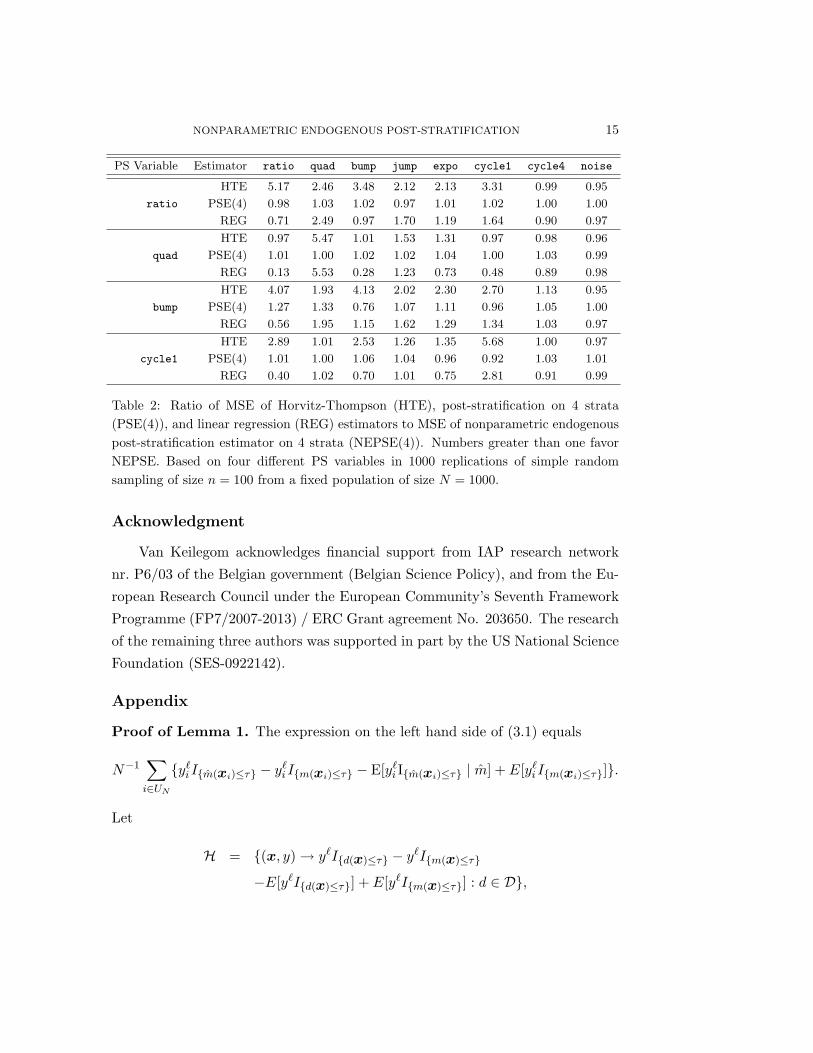
NONPARAMETRIC ENDOGENOUS POST-STRATIFICATION 15
PS Variable Estimator ratio quad bump jump expo cycle1 cycle4 noise
HTE 5.17 2.46 3.48 2.12 2.13 3.31 0.99 0.95
ratio PSE(4) 0.98 1.03 1.02 0.97 1.01 1.02 1.00 1.00
REG 0.71 2.49 0.97 1.70 1.19 1.64 0.90 0.97
HTE 0.97 5.47 1.01 1.53 1.31 0.97 0.98 0.96
quad PSE(4) 1.01 1.00 1.02 1.02 1.04 1.00 1.03 0.99
REG 0.13 5.53 0.28 1.23 0.73 0.48 0.89 0.98
HTE 4.07 1.93 4.13 2.02 2.30 2.70 1.13 0.95
bump PSE(4) 1.27 1.33 0.76 1.07 1.11 0.96 1.05 1.00
REG 0.56 1.95 1.15 1.62 1.29 1.34 1.03 0.97
HTE 2.89 1.01 2.53 1.26 1.35 5.68 1.00 0.97
cycle1 PSE(4) 1.01 1.00 1.06 1.04 0.96 0.92 1.03 1.01
REG 0.40 1.02 0.70 1.01 0.75 2.81 0.91 0.99
Table 2: Ratio of MSE of Horvitz-Thompson (HTE), post-stratification on 4 strata(PSE(4)), and linear regression (REG) estimators to MSE of nonparametric endogenouspost-stratification estimator on 4 strata (NEPSE(4)). Numbers greater than one favorNEPSE. Based on four different PS variables in 1000 replications of simple randomsampling of size n = 100 from a fixed population of size N = 1000.
Acknowledgment
Van Keilegom acknowledges financial support from IAP research network
nr. P6/03 of the Belgian government (Belgian Science Policy), and from the Eu-
ropean Research Council under the European Community’s Seventh Framework
Programme (FP7/2007-2013) / ERC Grant agreement No. 203650. The research
of the remaining three authors was supported in part by the US National Science
Foundation (SES-0922142).
Appendix
Proof of Lemma 1. The expression on the left hand side of (3.1) equals
N−1∑i∈UN
{y`i I{m(xi)≤τ} − y`i I{m(xi)≤τ} − E[y`i I{m(xi)≤τ} | m] + E[y`i I{m(xi)≤τ}]}.
Let
H = {(x, y)→ y`I{d(x)≤τ} − y`I{m(x)≤τ}
−E[y`I{d(x)≤τ}] + E[y`I{m(x)≤τ}] : d ∈ D},

NONPARAMETRIC ENDOGENOUS POST-STRATIFICATION 16
where D is defined as in assumption 3.1.4.
In a first step we will show that the class H is Donsker. From Theorem 2.5.6
in van der Vaart and Wellner (1996), it follows that it suffices to show that∫ ∞0
√logN[ ](λ,H, ‖ · ‖2) dλ <∞. (A.1)
From assumption 3.1.4 we know that the class
F = {(x, y)→ y`I{d(x)≤τ} : d ∈ D}
satisfies (A.1) with H replaced by F , and hence the same holds for H itself, since
the three other terms in H do not change its bracketing number.
Let
h(x, y) = y`(I{m(x)≤τ} − I{m(x)≤τ}
)− E
[y`(I{m(x)≤τ} − I{m(x)≤τ}
)∣∣∣ m] ,where (x, y) is independent of the fit, m(·). Then
Var(h(x, y) | m
)= Var
(y`(I{m(x)≤τ} − I{m(x)≤τ}
)∣∣∣ m)≤ E
[(y`(I{m(x)≤τ} − I{m(x)≤τ}
))2∣∣∣∣ m]
= E[y2`(I{m(x)≤τ} − I{m(x)≤τ}
)2∣∣∣ m]= E
[E[y2`(I{m(x)≤τ} − I{m(x)≤τ}
)2∣∣∣ m,x]∣∣∣ m]= E
[E[y2` | m,x]
(I{m(x)≤τ} − I{m(x)≤τ}
)2∣∣∣ m]= E
[E[y2` | x]
(I{m(x)≤τ} − I{m(x)≤τ}
)2∣∣∣ m]≤ K1 {Pr(m(x) ≤ τ,m(x) > τ | m)
+ Pr(m(x) > τ,m(x) ≤ τ | m)} , (A.2)
where K1 is given in assumption 3.1.5. Let ε > 0 be given. By assumption 3.1.1,
F (u) = Pr(m(x) ≤ u) is uniformly continuous, so there exists δ > 0 such that
|u1−u2| ≤ δ implies |F (u1)−F (u2)| < ε. We will show that Pr(m(x) ≤ τ,m(x) >

NONPARAMETRIC ENDOGENOUS POST-STRATIFICATION 17
τ | m) = op(1). Consider
Pr(
Pr(m(x) ≤ τ,m(x) > τ | m) > ε)
≤ Pr(
Pr(m(x) ≤ τ,m(x) > τ | m) > ε, supx|m(x)−m(x)| ≤ δ
)+ Pr
(supx|m(x)−m(x)| > δ
)≤ Pr
(Pr(m(x)− δ ≤ τ,m(x) > τ | m) > ε
)+ o(1)
= Pr(
Pr(m(x)− δ ≤ τ,m(x) > τ) > ε)
+ o(1)
= I{F (τ+δ)−F (τ)>ε} + o(1) = o(1), (A.3)
by choice of δ, where the second inequality follows from assumption 3.1.3. Simi-
larly,
Pr(m(x) > τ,m(x) ≤ τ | m) = op(1). (A.4)
For fixed η > 0, λ > 0 consider
Pr(N1/2|Aτ`(m)− E[y`i I{m(xi)≤τ} | m]−Aτ`(m) + ατ`(m)| > λ
)= Pr
N−1/2
∣∣∣∣∣∣∑i∈UN
h(xi, yi)
∣∣∣∣∣∣ > λ
≤ Pr
N−1/2
∣∣∣∣∣∣∑i∈UN
h(xi, yi)
∣∣∣∣∣∣ > λ,Var(h(x, y) | m) < η, m ∈ D
+ Pr
N−1/2
∣∣∣∣∣∣∑i∈UN
h(xi, yi)
∣∣∣∣∣∣ > λ,Var(h(x, y) | m) ≥ η, m ∈ D
+ Pr (m /∈ D)
≤ Pr
suph∈H,Var(h)<η
N−1/2
∣∣∣∣∣∣∑i∈UN
h(xi, yi)
∣∣∣∣∣∣ > λ
+ Pr
(Var(h(x, y) | m) ≥ η
)+ Pr (m /∈ D)
= d1N + d2N + d3N .
As N →∞, d1N = o(1) as η ↓ 0 by Corollary 2.3.12 in van der Vaart and Wellner

NONPARAMETRIC ENDOGENOUS POST-STRATIFICATION 18
(1996) and the fact that H is Donsker. Also, d2N = o(1) by the arguments in
(A.2)–(A.4), and d3N = o(1) by assumption 3.1.4. This establishes (3.1), and
similar arguments verify (3.2).
Proof of Theorem 1. Note that ANh`(M) = Aτh`(M) − Aτh−1`(M) and
Anh`(M) = Anτh`(M)−Anτh−1`(M), for M = {m, m}. Let
αh`(m) = ατh`(m)− ατh−1`(m) = E[y`i I{τh−1<m(xi)≤τh}].
Then, applying Lemma 1 to two consecutive boundary values, τh−1 and τh, we
have that the difference of the expressions is
ANh`(m)− E[y`i I{τh−1<m(xi)≤τh} | m]−ANh`(m) + αh`(m) = op(N−1/2), (A.5)
and
Anh`(m)− E[y`i I{τh−1<m(xi)≤τh} | m]−Anh`(m) + αh`(m) = op(n−1/2). (A.6)
Given (A.5) and (A.6), the remainder of the proof is very similar to the
corresponding proof in Breidt and Opsomer (2008). We mention highlights of
that proof (in the NEPSE context) and omit much of the detail. Begin by
defining ah = ANh0(m) − Anh0(m) and bh = ANh1(m) − Anh1(m). Calculation
of appropriate covariances shows that ah = Op(n−1/2
)and bh = Op
(n−1/2
). By
arguments similar to those in (A.2),
E[{
E[y`i I{τh−1<m(xi)≤τh} | m]− αh`(m)}2]
≤ E[K1
{Pr(τh−1 < m(xi) ≤ τh,m(xi) > τh | m)
+ Pr(τh−1 < m(xi) ≤ τh,m(xi) ≤ τh−1 | m)
+ Pr(m(xi) > τh, τh−1 < m(xi) ≤ τh | m)
+ Pr(m(xi) ≤ τh−1, τh−1 < m(xi) ≤ τh | m)}]. (A.7)
We want to show that (A.7) converges to 0 as n → ∞. Note that for a given

NONPARAMETRIC ENDOGENOUS POST-STRATIFICATION 19
ε > 0,
Pr(
Pr(τh−1 < m(xi) ≤ τh,m(xi) > τh | m) > ε)
≤ Pr(
Pr(m(xi) ≤ τh,m(xi) > τh | m) > ε)
= o(1),
by (A.3). Similar reasoning shows that each of the terms inside the expectation in
(A.7) is op(1). By uniform integrability, (A.7) is o(1). Thus, E[y`i I{τh−1<m(xi)≤τh} |m] converges to αh`(m) in mean square, and hence in probability.
Next,
ANh`(m)− αh`(m) = Op
(N−1/2
)and Anh`(m)− αh`(m) = Op
(n−1/2
)by the central limit theorem. Further note that Anhl(m) and ANhl(m) are Op(1)
by the weak law of large numbers.
Since αh0(m) > 0 by assumption 3.1.1, we have
1Anh0(m)
=1
αh0(m)+ op(1). (A.8)
We substitute (A.5), (A.6), and (A.8), and apply the established order results to
show that the NEPSE error,
µy(m)− yN =H∑h=1
{ANh0(m)Anh1(m)−Anh0(m)ANh1(m)
Anh0(m)
},
can be rewritten as
µy(m)− yN (A.9)
=H∑h=1
{αh1(m)αh0(m)
(ANh0(m)−Anh0(m))− (ANh1(m)−Anh1(m))}
+ op
(n−1/2
),
showing the asymptotic distribution is the same as that obtained when m(·) is
known.
To derive the asymptotic distribution, we apply the central limit theorem to
(A.9) and refer to previously mentioned covariance computations. The limiting
distribution of the NEPSE error is normal with mean zero and the variance is

NONPARAMETRIC ENDOGENOUS POST-STRATIFICATION 20
approximated by
Var (µy(m)− yN )
' − 1n
(1− n
N
) H∑h=1
α2h1(m)αh0(m)
+1n
(1− n
N
)( H∑h=1
αh1(m)
)2
+ Var (yπ − yN )
=1n
(1− n
N
){−
H∑h=1
α2h1(m)αh0(m)
+ [E(yi)]2 + Var (yi)
}.
By definition of expectation given an event,
αh1(m)αh0(m)
= E[yi | τh−1 < m(xi) ≤ τh]
and
E(y2i ) =
H∑h=1
αh0(m){
Var(yi | τh−1 < m(xi) ≤ τh) + [E(yi | τh−1 < m(xi) ≤ τh)]2},
from which the variance given in Theorem 1 immediately follows.
Proof of Theorem 2. With only notational changes to indicate NEPSE results,
this proof is identical to the corresponding EPSE proof of Breidt and Opsomer
(2008). Note that ANh`(m) P→ αh`(m) and Anh`(m) P→ αh`(m) as n,N → ∞by the weak law of large numbers, and E[y`i I{τh−1<m(xi)≤τh} | m] P→ αh`(m) for
` = 0, 1, 2 by the arguments following (A.7). Using equations (A.5) and (A.6),
the expression given for Vym in (3.3) converges in probability to
H∑h=1
αh0(m)
{αh2(m)αh0(m)
−(αh1(m)αh0(m)
)2}
from which the result follows by Slutsky’s Theorem and Theorem 1.
References
Breidt, F. J. and J. D. Opsomer (2008). Endogenous post-stratification in
surveys: classifying with a sample-fitted model. Annals of Statistics 36,
403–427.

NONPARAMETRIC ENDOGENOUS POST-STRATIFICATION 21
Czaplewski, R. L. (2010). Complex sample survey estimation in static state-
space. Gen. Tech. Rep. RMRS-GTR-xxx (in press), U.S. Department of
Agriculture, Forest Service, Rocky Mountain Research Station, Fort Collins,
CO.
Fan, J., N. E. Heckman, and M. P. Wand (1995). Local polynomial kernel re-
gression for generalized linear models and quasi-likelihood functions. Jour-
nal of the American Statistical Association 90 (429), 141–150.
Frayer, W. E. and G. M. Furnival (1999). Forest survey sampling designs: A
history. Journal of Forestry 97, 4–8.
Green, P. J. and B. W. Silverman (1994). Nonparametric Regression and Gen-
eralized Linear Models. Washington, D. C.: Chapman and Hall.
McCullagh, P. and J. A. Nelder (1989). Generalized Linear Models (2 ed.).
London: Chapman and Hall.
Moisen, G. G. and T. S. Frescino (2002). Comparing five modelling techniques
for predicting forest characteristics. Ecological Modelling 157, 209–225.
Ruppert, D., M. P. Wand, and R. J. Carroll (2003). Semiparametric Regression.
Cambridge, UK: Cambridge University Press.
Sarndal, C. E., B. Swensson, and J. Wretman (1992). Model Assisted Survey
Sampling. New York: Springer-Verlag.
Silverman, B. W. (1999). Density Estimation for Statistics and Data Analysis.
Chapman and Hall Ltd.
Simonoff, J. S. (1996). Smoothing Methods in Statistics. New York: Springer-
Verlag.
van der Vaart, A. W. and J. A. Wellner (1996). Weak Convergence and Em-
pirical Processes. Springer-Verlag Inc.
Department of Statistics, Colorado State University, Fort Collins, CO 80523,
U.S.A.
E-mail: [email protected]
Department of Statistics, Colorado State University, Fort Collins, CO 80523,
U.S.A.

NONPARAMETRIC ENDOGENOUS POST-STRATIFICATION 22
E-mail: [email protected]
Department of Statistics, Colorado State University, Fort Collins, CO 80523,
U.S.A.
E-mail: [email protected]
Institute of Statistics, Universite catholique de Louvain, Voie du Roman Pays
20, B-1348 Louvain-la-Neuve, Belgium.
E-mail: [email protected]


![Willkommen beim Reichert Verlag · 14 Marcel van Ackeren – Jan Opsomer Beitrag auf Marc Aurel (reydaMs-schils [2005]).21 Ebenfalls jüngst zum Thema erschienen ist eine neue Studie](https://static.fdocuments.net/doc/165x107/6064fa0252a1995e0e2a1e81/willkommen-beim-reichert-verlag-14-marcel-van-ackeren-a-jan-opsomer-beitrag-auf.jpg)