D The Effect of Competition and Capacity on Intermediation ...

13

Int. Journal of Economics and Management 14 (1): 13-26 (2020)

IJEM International Journal of Economics and Management

Journal homepage: http://www.ijem.upm.edu.my

The Effect of Competition and Capacity on Intermediation Cost:

A Country Level Study

MOCHAMMAD DODDY ARIEFIANTOa*, RINDANG WIDURIa, EDI ABDURACHMANb AND IRWAN TRINUGROHOc

aAccounting Department, BINUS Graduate Program-Master Accounting,

Bina Nusantara University, Jakarta bManagement Department, BINUS Business School-Doctor of Research in Management,

Bina Nusantara University, Jakarta cFaculty of Economics and Business, Universitas Sebelas Maret, Jl. Ir. Sutami 36A,

57126 Surakarta, Indonesia

ABSTRACT

We investigate the determinants of bank intermediation cost at the country level by focusing

on the role of competition and bank capacity in a cross-country study. Using the Global

Financial Development Database – GFDD, we estimate a regression of net interest margins

to a set of variables specifically proxies for competition, capacity and some controlling

variables. Panel data econometric techniques employed are fixed effect, random effect and

pooled OLS. We find that intermediation cost is positively associated with capital adequacy,

overhead cost, return on equity and ZSCORE. On the other hand, it is negatively associated

with loan to deposit ratio, deposit to GDP and GDP per capita. Finally, our study has shown

that income level and financial deepening have positive impact on intermediation efficiency.

JEL Classification: G21, G18, L22, C23

Keywords: Bank Intermediation Cost; Competition; Capacity; Panel Data Econometrics

Article history:

Received: 18 August 2019

Accepted: 20 January 2020

* Corresponding author: Email: [email protected]

D

14

International Journal of Economics and Management

INTRODUCTION

Banks are a critical component in the financial system in many countries. In addition to channeling idle funds

to productive needs (from surplus units to deficit units) in the economy; banks also perform brokerage function

and asset transformation as well as information processing (Greenbaum et al., 2019). By doing brokerage

function, banks help reduce transaction cost, project screening to eliminate adverse selection, financial advice

and origination. On the other hand, by conducting asset transformation, banks improve monitoring (thus

mitigating moral hazard) and liquidity creation. The importance of banks can vary from country to country

depending on the financial structure (Demirguc-Kunt and Levine, 2004).

Subsequently, the bank intermediation cost is affected by internal and external factors. From internal

perspective, intermediation cost could be influenced by targeted return by the management and shareholders

(with accompanied risk appetite) in excess of operating cost and credit cost (Freixas and Rochet, 2008).

Certainly, lending and deposit spread is not decided in the vacuum, instead it is an outcome of strategic

interaction with other industry players which is a market/competition outcome (Van Hoose, 2010).

The external factors are ranging from macro economy condition, regulation and banking penetration. It

could also result from some qualitative factors such as regulation, culture and political set up (Barth et al., 2008).

Regulators in some countries restrain interest rate (for both deposit and lending) as they perceived it as usury.

In other countries, high lending spread has been subjected to political scorn; bankers are perceived to be greedy

and the conduct would harm economic growth.

This study focuses on the conduct and performance at country level rather than individual bank level.

We are also motivated by the existence of a comprehensive (and open access) country level financial sector

database; released relatively recent by World Bank in 2013: Global Financial Development Database - GFDD

(see Cihak et al., 2012 for description of the database). As of July 2019, the database contained 117 annual data

series from 1960 – 2017 of 214 countries.

We use data from GFDD in our empirical model. Our sample comprises (initially) of annual data of 12

series from 1996 to 2016 of 212 countries. Variants of panel data regressions (Pooled OLS; Fixed Effect and

Random Effect) are used to estimate the empirical relationship of intermediation cost with various variables. In

addition to baseline regressions, we elaborate the model further to include categoric variables: (a) country

income stage category and (b) crisis episodes dummies. In this regard, we hope to obtain richer insights from

the analysis.

Banking industry is the backbone of financial system in many developing countries (Demirguc-Kunt and

Levine, 2004). Therefore, it is very important to gain a good understanding of how the industry behaves

especially when it comes to intermediation. Literature on intermediation cost has been quite extensive.

Nevertheless, many studies are using banks level data. We argue that a study that focus on country level data is

also important; as it will better reveal how banking operates as a system. Country system comparisons (a more

macroeconomic perspective) should yield high level insights useful for policy making.

To our knowledge our study is the first study on intermediation cost using GFDD database. Our coverage

of study (in terms of number of countries) is also one of the most extensive; combining countries from various

level of development. Therefore, considering the more macro perspective approach and extensive dataset; we

think that the study could add significant value added to the literature.

After introduction in section 1, literature review is presented in section 2. We model the relationship of

cost intermediation and capacity to lending, competition and other controlling variables in section 3. In the

methodology section, we also lay out the hypotheses and techniques to check robustness. In section 4, we present

the estimation results, derive important insights and relate them with existing literature. Section 5 presents the

conclusion of the study.

LITERATURE REVIEW

Previous studies on bank cost of intermediation could be performed from various approaches: Finance,

Industrial Organization, Bank Management, Monetary Theory and Financial Regulation. The need for multi

discipline approach stem from the nature of bank as unique. Unlike other financial firm, bank is a key player in

monetary policy transmission (Walsh, 2010) and a country financial stability (Narain et al., 2013). Beck et al.

15

The Effect of Competition and Capacity on Intermediation Cost: A Country Level Study

(2006) document cross country evidence of banking industry behavior that not only directed by private decision

but also substantially from public policy.

One benchmark model for cost of intermediation (in which our study based on) is due to Ho and Saunders

(1981). Here the cost of intermediation (proxied by ratio of net interest income to earning assets; Net Interest

Margin-NIM) is modeled as a channeling fund activity performed by risk averse banks. Banks accept random

supplies of fund; and subsequently lend the funds to random loan demands. Banks required a positive margin

to perform this function since they deal with uncertainty on both sides of their balance sheet. Based on theoretical

modeling (known as Dealership Model) and empirical estimation, they conclude that there are four factors that

affect NIM which are the degree of managerial risk aversion, the size of transactions, market structure, and the

variance of the market interest rate.

This seminal study sparks subsequent expansion both theoretical and empirical. Allen (1988) expand the

model by including possible interest margin reducing effect from diversification of products. Angbazo (1997)

model the impact of credit risk and interest rate risk, as well as the interaction of those types of risk. Saunders

and Schumacher (2000); add the role of capital ratio, market power and macroeconomic volatility to the model

and found empirical support from cross country data of European and US banks.

Maudos and Guevara (2004) include operating costs and market power: Lerner index as additional key

factors of NIM. Valverde and Fernandez (2007) developed a model by adopting New Industrial Organization

approach in bank product specialization context and tested to European Banking. Maudos and Solis (2009) unify

the previous works in which NIM is modelled to include the impact of operating cost, credit risk, interest rate

risk, market power and macroeconomic volatility. They find empirical support for their model with Mexican

banking data. Kasman et al. (2010) incorporate the impact of banking consolidation by using natural

experiments of country admittance to European Union to Interest Margin setting. Here they found evidences

that lowering of barrier of entry and consolidation improved intermediation efficiency (by lowering NIM). More

recently Entroph et al. (2015) modify Ho and Saunders (1981) work by separating risk attribution (credit and

liquidity) of NIM to interest revenue and interest expense component. They found evidences from German

banking that credit risk priced in individually from assets side to the NIM.

There are some applications of extended Ho and Saunders (1981) model to empirical works in particular

country setting. Trinugroho et al. (2014) study the post crisis 1997 Indonesian banking industry with model

extension to include structure of loan portfolio (small and property categories) and ownership. Were and

Wambua (2014), Hussain (2014) and Nuhiu et al. (2017), test empirically the model to developing countries in

the context of heavily concentrated banking industry in Kenya, Pakistan and Kosovo respectively. On regional

perspectives, empirical works have also been performed by Martinez and Peria (2004) on Latin America Banks,

Angori et al. (2019) on European Banks and Mustafa and Toci (2018) on CESEE countries. One of the most

extensive cross-country bank level empirical has been done by Demirguc-Kunt et al. (2004) which involve 1400

banks from 72 countries.

From a management perspective, bank is a firm whose business mainly involving taking deposits and

subsequently lending them. In doing so, banks expose themselves to various risks mainly duration, credit

quality, currency and liquidity. Bank managers then try to optimize these factors to get required return by their

shareholders (Koch et al., 2014). Research on interest margin determination can also be viewed from this

managerial perspective, in which interest margin is one measure of profitability (as an alternative to return on

assets and return on equity) to cover operational cost, business risk provision and required rate of return to

shareholders. Variability of impact from these factors in turn depends on level of financial development,

regulatory set up, competition and macroeconomic condition (Demirguc-Kunt and Huizinga, 2000)

A more recent comprehensive study is done by Athanasoglou et al. (2008). Building on Demirguc-Kunt

and Huizinga (2000) model, they group the factors into Bank Specific, Industry Specific and Macroeconomic

and tested for possible (time) persistence of profit measures. Application to a sample of Greek banks, they find

evidence of profit persistency and the significant role of bank specific factors and asymmetric effect of

macroeconomics. Ariss (2010) applies a tripod framework: simultaneous determination of profitability, stability

and competition model. Based on empirical application on banks in 60 developing countries, she find evidence

that market power positively affects profit.

Dietrich and Wanzenried (2011) examine a panel data of 453 Switzerland banks which includes crisis

period: 2008. They find that capital and business mix are main determinant of profit which altered by Crisis.

Yong Tan (2016), studies banks in China in which he finds positive impact of market power, risk taking and

16


banking development to profitability. Al Harbi (2019) study conventional banks from 52 OIC countries and he

find that foreign ownership and off-balance sheet improved profitability. Profitability is also found to be

procyclical. Berger et al. (2004) document a global trend toward consolidation of banking industry; therefore,

for banks exercising greater market power. The major forces behind the trend are relationship banking (Berger

and Udell, 2002), progress in information and financial technology (Berger, 2003) and economies of scale

(Hughes and Mester, 1998).

There are opposing views on the impact of competition on banking performance and finally to financial

stability (Boyd and DeNicolo, 2005). One strain is sympathetic toward competition as standard economic theory

affirms that it will bring goods to all parties: customers, banks, regulator and public. In competitive market

banks would provide the necessary service: liquidity, productive financing and risk management with normal

margin regardless the business cycle. This in turn would dampen the volatility of real sector (Beck et al., 2006;

Larrain, 2006). The opposing stance proposes that too intense competition would encourage risk taking that

might harm profitability; hence subsequently capital that renders banking industry to be vulnerable to economic

shock (Soedarmono et al., 2013). The outcome is undesirable as banks have a tendency to pose huge fiscal risk

due to perception of contagion and too big to fail. Therefore, public approach to banking industry tends to be

heavy handed (Fischer and Pfeil, 2003).

Rather than using concentration-based measures to gauge the degree of competition, we prefer to use

behavioral indicators. There are several established techniques to measure degree of competition in banking;

known in New Empirical Industrial Organization-NEIO (Degryse et al., 2008). Boone (2008) introduces a

measure of competition that stems from profit elasticity due to marginal cost. As competition gets more intense,

coefficient of marginal cost will rise and adversely affect profit.

Bresnahan (1982) and Lau (1982) develop Lerner Index which measures the extent to which price

exceeding marginal cost hence showing the degree of market power exercised. This approach is also known as

conjectural variation method. Lastly, there is also H Index which measures the sum of elasticity of interest

revenue to various input and bank specific factors. The index, which is developed by Panzar and Rosse (1987),

ranges from 0 to 1 with higher number indicates more competition.

Rosseau and Wachtel (2000) find that the relationship of financial sector and growth might be more

complicated than commonly assumed. Financial development might promote growth; but the causality is open

for the reversed. Nevertheless, more recent empirical studies has moved toward the former: financial

development facilitates growth (Degryse et al., 2008; Sahay et al., 2015). This is the stance used in our study:

factors that help financial development will trigger more growth supportive behavior like lower intermediation

margin.

METHODOLOGY

In this study, we attempt to model the relationship of several major factors to intermediation cost of banks based

on Saunders and Schumacher (2000). The intermediation cost is proxied by ratio of Net Interest Income to

Earning Assets (Net Interest Margin; NIM). Specifically, we focus on two variables of interests that drive this

cost which are competition and capacity to lend (proxied by CAR and NPL). We include some controlling

variables comprises of Bank Internal Characteristics, Financial Stability and Structural Factors.

We model the estimated relationship as a linear form as follows:

𝐼𝐶𝑖𝑡 = 𝛼0 +∑𝛼𝑛𝐶𝑇𝐿𝑛𝑖𝑡 +

2

𝑛=1

𝛼3𝐶𝑂𝑀𝑃𝑖𝑡 +∑𝛼𝑛𝐶𝐻𝐴𝑅𝑛𝑖𝑡 +

5

𝑛=4

∑𝛼𝑛𝐹𝑆𝑛𝑖𝑡 +

7

𝑛=6

∑𝛼𝑛𝑆𝐹𝑛𝑖𝑡 +

9

𝑛=8

𝑢𝑖𝑡

𝑢𝑖𝑡 = 𝑣𝑖 + 𝑒𝑖𝑡

Where IC is Intermediation Cost (here proxied as Net Interest Margin; NIM). As regressors we use

Capacity to Lend proxies (CTL), Competition Indicators (COMP), Bank Internal Characteristic (CHAR),

Financial Stability indicators (FS) and Structural Factors (SF). The residual of regression is a composite error

term comprised of vi is cross section residual component (Fixed and/or Random Effect) and idiosyncratic

residual component (eit).

17


Table 1 Variable, Proxies and Expected Sign

This table presents the variables and their proxies. The hypotheses for explanatory variables are presented in the form

of expected algebraic sign. No Variables Proxies Expected Sign (Hypotheses)

1 Intermediation Cost (Dependent Variable) -Net Interest Margin (NIM)

2 Capacity to Lend -Capital Adequacy Ratio (CAR), and

-Loan to Deposit Ratio (LDR)

Positive

Negative 3 Competition Indicators -Boone Indicators (BOONE); or

-Lerner Index (LERNER); or -H Statistics (HINDEX)

Positive

Positive Negative

4 Characteristics (CHAR) -Overhead Cost to Total Asset (OHCTOTA), and

-Return On Equity (ROE)

Positive

Positive 5 Financial Stability (FS) -Stock Price Volatility (STOCKVLTY)

-Bank Z Score (ZSCORE)

Negative

Negative

6 Structural Factors (SF) - Ratio of Deposit in Banks to GDP (DEPOTOGDP)

- GDP per Capita (In Constant USD 2005,

GDPPERCAP)

Negative

Negative

Table 1 provides the expected sign of explanatory variables. Our variables of interest are Capacity of

Lending (CAR and LDR) and Competition proxy (BOONE, HINDEX and LERNER). The sign hypotheses are

explained in literature review section. We expect CAR to have a positive association with NIM; while LDR to

have a negative one. Due to their construction; competition proxies have different expected sign hypotheses.

Nevertheless, we generally expect that higher competition intensity to be associated with lower NIM. The detail

of each proxy computation (definition) is provided in the table 2.

In the estimation model, we assume only cross section effect both for fixed effect and random effect. The

choice only to include cross section is to avoid possible collinearity with the time variant exogenous variables

like STOCKVLTY, ZSCORE, DEPOTOGDP and GDPPERCAP.

All data are obtained from Global Financial Database (GFDD) from World Bank. Initially this data

contains information 14 series of 214 countries (or equivalent concept) with annual frequency from 1990 to

2016 (5564 observations). For this study we carefully inspect the data hence the final dataset become unbalanced

panel and the number of observations is significantly reduced to 1889.

The models are estimated using Fixed Effect (FE), Random Effect (RE) and pooled OLS. We then review

the estimation results based on specification adequacy criteria (see Pesaran, 2015). There are five statistics used

to measure the goodness of fit of the estimations results and specifications. R Square and F Statistics are used

to gauge the overall adequacy of variance of independent variables to explain variance of dependent variables.

We start regressions with Fixed Effect and Random Effect; then we include Pooled OLS as a comparison.

As for specification test, we employ a Likelihood Ratio based statistic to test for appropriateness of fixed

effect model against pooled OLS. We use a Lagrange Multiplier based statistic to test for appropriateness of

random effect model against pooled OLS. Lastly, we test appropriateness of random effect model against fixed

effect using Hausman Test.

We further elaborate the model by taking effect of country income categories and bank crisis. We model

the impact as to the constant of the regressions. To account the effect of bank crisis period to the model, we

include the dummy bank crisis (that is Bank Crisis is 1 if a country in a particular period/s experiencing bank

crisis; zero otherwise). Lastly, we re-estimate the model by including dummy variables of country category with

low income taking role (L) as reference. There are three dummy variables: D_LM (low-Middle income

countries), D_UM (Upper Middle-Income Countries), D_H (High Income Countries)1.

1 This is a moving classification based on Gross National Income per Person using ATLAS methods; Classification threshold are adjusted

for inflation annually using the SDR deflator. As of July 2018, low-income economies are defined as those with a GNI per capita of $995 or less in 2017; lower middle-income economies are those with a GNI per capita between $996 and $3,895; upper middle-income economies

are those between $3,896 and $12,055; high-income economies are those with a GNI per capita of $12,055 or more.

18


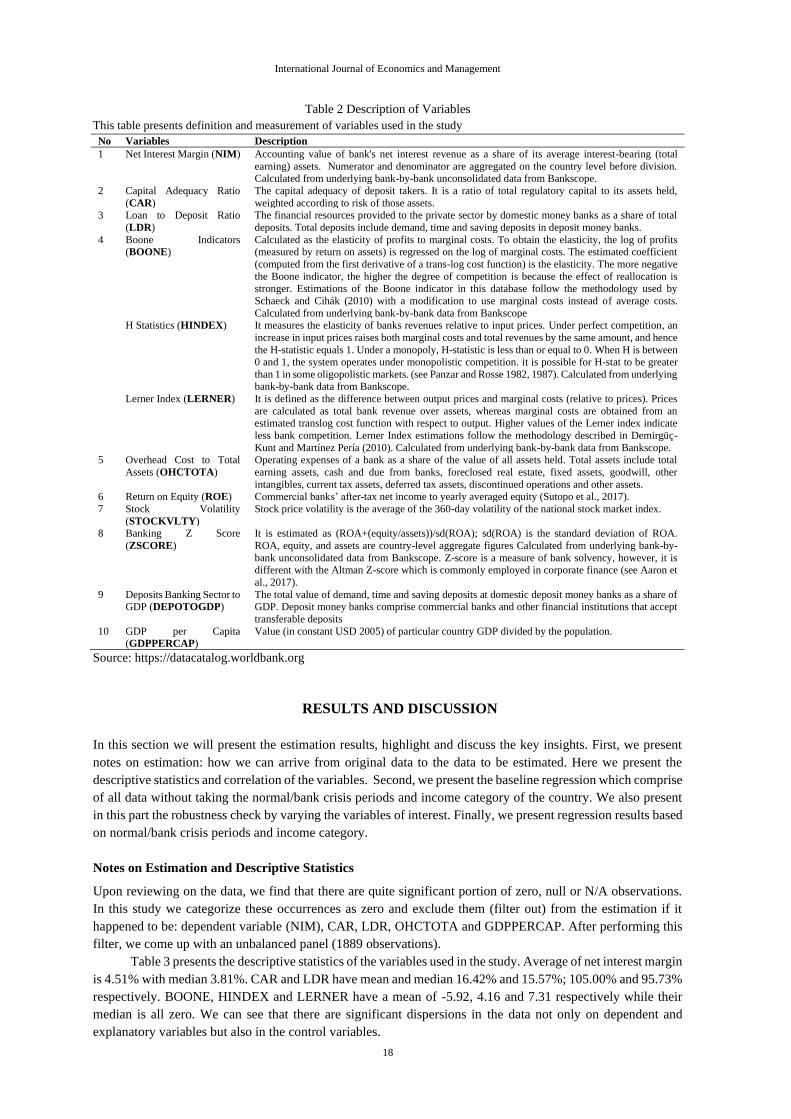
Table 2 Description of Variables

This table presents definition and measurement of variables used in the study

No Variables Description

1 Net Interest Margin (NIM) Accounting value of bank's net interest revenue as a share of its average interest-bearing (total

earning) assets. Numerator and denominator are aggregated on the country level before division. Calculated from underlying bank-by-bank unconsolidated data from Bankscope.

2 Capital Adequacy Ratio

(CAR)

The capital adequacy of deposit takers. It is a ratio of total regulatory capital to its assets held,

weighted according to risk of those assets. 3 Loan to Deposit Ratio

(LDR)

The financial resources provided to the private sector by domestic money banks as a share of total

deposits. Total deposits include demand, time and saving deposits in deposit money banks.

4 Boone Indicators (BOONE)

Calculated as the elasticity of profits to marginal costs. To obtain the elasticity, the log of profits (measured by return on assets) is regressed on the log of marginal costs. The estimated coefficient

(computed from the first derivative of a trans-log cost function) is the elasticity. The more negative

the Boone indicator, the higher the degree of competition is because the effect of reallocation is stronger. Estimations of the Boone indicator in this database follow the methodology used by

Schaeck and Cihák (2010) with a modification to use marginal costs instead of average costs.

Calculated from underlying bank-by-bank data from Bankscope H Statistics (HINDEX) It measures the elasticity of banks revenues relative to input prices. Under perfect competition, an

increase in input prices raises both marginal costs and total revenues by the same amount, and hence

the H-statistic equals 1. Under a monopoly, H-statistic is less than or equal to 0. When H is between

0 and 1, the system operates under monopolistic competition. it is possible for H-stat to be greater

than 1 in some oligopolistic markets. (see Panzar and Rosse 1982, 1987). Calculated from underlying bank-by-bank data from Bankscope.

Lerner Index (LERNER) It is defined as the difference between output prices and marginal costs (relative to prices). Prices

are calculated as total bank revenue over assets, whereas marginal costs are obtained from an estimated translog cost function with respect to output. Higher values of the Lerner index indicate

less bank competition. Lerner Index estimations follow the methodology described in Demirgüç-

Kunt and Martínez Pería (2010). Calculated from underlying bank-by-bank data from Bankscope. 5 Overhead Cost to Total

Assets (OHCTOTA)

Operating expenses of a bank as a share of the value of all assets held. Total assets include total

earning assets, cash and due from banks, foreclosed real estate, fixed assets, goodwill, other

intangibles, current tax assets, deferred tax assets, discontinued operations and other assets. 6 Return on Equity (ROE) Commercial banks’ after-tax net income to yearly averaged equity (Sutopo et al., 2017).

7 Stock Volatility

(STOCKVLTY)

Stock price volatility is the average of the 360-day volatility of the national stock market index.

8 Banking Z Score

(ZSCORE)

It is estimated as (ROA+(equity/assets))/sd(ROA); sd(ROA) is the standard deviation of ROA.

ROA, equity, and assets are country-level aggregate figures Calculated from underlying bank-by-

bank unconsolidated data from Bankscope. Z-score is a measure of bank solvency, however, it is different with the Altman Z-score which is commonly employed in corporate finance (see Aaron et

al., 2017).

9 Deposits Banking Sector to GDP (DEPOTOGDP)

The total value of demand, time and saving deposits at domestic deposit money banks as a share of GDP. Deposit money banks comprise commercial banks and other financial institutions that accept

transferable deposits

10 GDP per Capita (GDPPERCAP)

Value (in constant USD 2005) of particular country GDP divided by the population.

Source: https://datacatalog.worldbank.org

RESULTS AND DISCUSSION

In this section we will present the estimation results, highlight and discuss the key insights. First, we present

notes on estimation: how we can arrive from original data to the data to be estimated. Here we present the

descriptive statistics and correlation of the variables. Second, we present the baseline regression which comprise

of all data without taking the normal/bank crisis periods and income category of the country. We also present

in this part the robustness check by varying the variables of interest. Finally, we present regression results based

on normal/bank crisis periods and income category.

Notes on Estimation and Descriptive Statistics

Upon reviewing on the data, we find that there are quite significant portion of zero, null or N/A observations.

In this study we categorize these occurrences as zero and exclude them (filter out) from the estimation if it

happened to be: dependent variable (NIM), CAR, LDR, OHCTOTA and GDPPERCAP. After performing this

filter, we come up with an unbalanced panel (1889 observations).

Table 3 presents the descriptive statistics of the variables used in the study. Average of net interest margin

is 4.51% with median 3.81%. CAR and LDR have mean and median 16.42% and 15.57%; 105.00% and 95.73%

respectively. BOONE, HINDEX and LERNER have a mean of -5.92, 4.16 and 7.31 respectively while their

median is all zero. We can see that there are significant dispersions in the data not only on dependent and

explanatory variables but also in the control variables.

https://datacatalog.worldbank.org/

19


Correlation is presented in Table 4 which shows that all bivariate correlation is within rule of thumb

(0.7). Pairwise correlation between DEPOTOGDP and GDPPERCAP is noteworthy (0.55). However, as we can

see later (in estimation results), it seems it does not cause significant problem. The correlation table has given

hindsight on possible sign of regressions. Here we have a positive correlation between NIM and CAR; NIM and

OHCTOTA and NIM and ROE. Negative correlations exist between NIM and LDR; NIM and STOCKVLTY,

NIM and DEPOTOGDP and GDPPERCAP.

This table reports descriptive statistics of variables. The statistics comprised of mean, median, maximum,

minimum, standard deviation, skewness, kurtosis and Jarque-Berra (to indicate deviation from normality)

Table 3 Descriptive Statistics

This table reports simple correlation (Pearson correlation) of variables used in the study. The presentation

of correlation takes form of lower half triangle.

Table 4 Correlation Table

Baseline Regression

Since we deal with unbalanced panel, we cannot rely on the use of two-way random effect (heterogeneity on

cross section and time simultaneously). Some diagnostic tests cannot also be performed. Therefore, we focus

only on heterogeneity among cross section (single effect): Fixed Effect and Random Effect with Pooled OLS as

additional reference.

We can see from Table 5, the specification test: Likelihood Ratio (LR) and Lagrange Multiplier (LM)

showed that both type cross section effects (Fixed and Random) are statistically significant. Hence FE and RE

estimates are preferable to Pooled OLS. Nevertheless, Hausman Test overwhelmingly rejected null hypotheses

no correlation between random component residual to idiosyncratic residual. This result leads to preference of

fixed effect over random effect.

As expected, sign of CAR coefficient estimations is all positive under all specification and competition

proxies. This is a quite robust findings in line with Ho and Saunders (1981) and Trinugroho et al. (2014) shows

that bank managers pass on their risk aversion to the customers. The liquidity proxy (LDR) has correct estimated

coefficients nevertheless they are either has a small economic impact (under pooled OLS and RE) or statistically

insignificant (under FE).

Mean Median Maximum Minimum Std. Dev. Skewness Kurtosis Jarque-Bera Probability

NIM 4.514 3.809 18.634 0.125 2.887 1.075 4.335 504.247 0.000

CAR 16.422 15.567 48.600 1.755 5.162 1.603 7.382 2319.867 0.000

LDR 105.002 95.725 879.662 15.335 62.189 5.611 56.469 234932.000 0.000

BOONE -5.922 0.000 160.741 -5981.630 138.432 -42.626 1840.109 266000000.000 0.000

HINDEX 4.159 0.000 92.500 -8.670 15.766 3.896 17.237 20732.820 0.000

LERNER 7.312 0.000 153.407 -160.869 15.697 1.845 21.608 28324.340 0.000

ROE 12.485 12.606 160.344 -117.673 14.050 -0.641 25.513 40019.980 0.000

OHCTOTA 3.661 2.807 81.900 0.041 3.437 8.395 159.484 1949524.000 0.000

ZSCORE 13.915 12.343 95.279 -0.241 9.345 1.723 8.584 3388.152 0.000

STOCKVLTY 14.228 14.222 99.030 0.000 13.444 1.022 5.233 721.430 0.000

DEPOTOGDP 56.540 44.973 472.049 0.000 52.698 3.214 17.301 19347.920 0.000

GDPPERCAP 17.258 8.313 111.968 0.218 20.610 1.712 5.879 1574.520 0.000

Correlation NIM CAR LDR BOONE HINDEX LERNER ROE OHCTOTA ZSCORE STOCKVLTY DEPOTOGDP GDPPERCAP

NIM 1.000

CAR 0.382 1.000

LDR -0.166 -0.141 1.000

BOONE -0.023 -0.045 0.009 1.000

HINDEX 0.054 0.015 -0.034 0.002 1.000

LERNER 0.051 0.063 -0.052 0.000 0.253 1.000

ROE 0.359 0.092 -0.155 -0.007 0.058 0.036 1.000

OHCTOTA 0.591 0.233 -0.087 -0.004 0.046 0.012 0.122 1.000

ZSCORE -0.117 -0.037 -0.079 -0.022 0.014 0.009 0.043 -0.166 1.000

STOCKVLTY -0.374 -0.294 0.168 0.020 -0.082 -0.067 -0.244 -0.182 -0.076 1.000

DEPOTOGDP -0.507 -0.153 -0.160 -0.023 -0.050 0.001 -0.168 -0.363 0.275 0.226 1.000

GDPPERCAP -0.587 -0.191 0.129 -0.011 -0.031 -0.058 -0.149 -0.393 0.102 0.273 0.552 1.000

20


The competition behavior proxies are statistically not significant under all specifications. This is quite

different with several benchmark studies that find competition as significant factor in decreasing the margin

(Saunders and Schumacher, 2000; Trinugroho et al., 2014; Entroph, 2015; Mustafa and Toci, 2018).

This table reports baseline regression results. Dependent variable (NIM) is regressed against capacity

proxies (NIM, LDR), competition proxies (BOONE, HINDEX and LERNER) and controlling variables. The

table presents estimated coefficients and p values in parentheses. Each regression (denotes in number in the

table header second line) corresponds with estimation technique (FE, RE and Pooled OLS) and competition

proxy. Statistical significance used: * at 10% level, ** at 5% level, *** at 1% level respectively.

Table 5 Baseline Regression Results

This table reports robustness check regression result for competition proxy: BOONE. Robustness check

was performed by sequential inclusion of variables of interest: CAR, LDR and Competition Proxy (BOONE,

HINDEX, LERNER). Each regression (denotes in number in the table header second line) corresponds with

estimation technique (FE, RE and Pooled OLS) and competition proxy. The report presents estimated

coefficients with p value in parentheses. Statistical significance used: * at 10% level, ** at 5% level, *** at 1%

level respectively.

No Variable/Proxies

1 2 3 4 5 6 7 8 9

1 CAR 0.053*** 0.053*** 0.053*** 0.068*** 0.067*** 0.068*** 0.096*** 0.097*** 0.097***

(0.000) (0.000) (0.000) (0.000) (0.000) (0.000) (0.000) (0.000) (0.000)

2 LDR -0.002 -0.002 -0.002 -0.002** -0.002** -0.002** -0.003*** -0.003*** -0.003***

(0.137) (0.136) (0.134) (0.014) (0.013) (0.014) (0.000) (0.000) (0.000)

3 BOONE 0.000 0.000 0.000

(0.000) (0.119) (0.000)

HINDEX -0.003 -0.003 0.000

(0.213) (0.174) (0.894)

LERNER -0.001 0.000 0.001

(0.602) (0.907) (0.720)

4 OHCTOTA 0.119** 0.119** 0.119** 0.140*** 0.141*** 0.140*** 0.285*** 0.286*** 0.286***

(0.046) (0.046) (0.046) (0.000) (0.000) (0.000) (0.003) (0.003) (0.003)

5 ROE 0.022*** 0.022*** 0.022*** 0.025*** 0.025*** 0.025*** 0.042*** 0.042*** 0.042***

(0.000) (0.000) (0.000) (0.000) (0.000) (0.000) (0.000) (0.000) (0.000)

6 STOCKVLTY 0.005 0.005 0.005 0.001 0.002 0.001 -0.020*** -0.020*** -0.020***

(0.314) (0.289) (0.316) (0.676) 0.646 0.679 (0.000) (0.000) (0.000)

7 ZSCORE 0.042** 0.042** 0.042 0.027*** 0.027*** 0.027*** -0.001 -0.001 -0.001

(0.019) (0.019) (0.019) (0.000) (0.000) (0.000) (0.910) (0.922) (0.921)

8 DEPOTOGDP -0.009** -0.009** -0.009** -0.011*** -0.011*** -0.011*** -0.009*** -0.009*** -0.009***

(0.026) (0.026) (0.027) (0.000) (0.000) (0.000) (0.000) (0.000) (0.000)

9 GDPPERCAP -0.051*** -0.051*** -0.051*** -0.051*** -0.051*** -0.051*** -0.037*** -0.037*** -0.037***

(0.000) (0.000) (0.000) (0.000) (0.000) (0.000) (0.000) (0.000) (0.000)

R2 0.844 0.844 0.844 0.282 0.281 0.281 0.624 0.624 0.624

F stat 66.393*** 66.415*** 66.306 81.867*** 81.648*** 81.481***346.969***346.549***346.569***

(0.000) (0.000) (0.000) (0.000) (0.000) (0.000) (0.000) (0.000) (0.000)

FE Test (Chi Square stat) 1657.034***1658.981*** 1656.305***

(0.000) (0.000) (0.000)

LM Test (RE Test)* 54.839*** 54.882*** 54.948***

*Cross Section Standardized Honda (Honda, 1991) (0.000) (0.000) (0.000)

Hausman Test 117.401***118.18*** 118.186***

(0.000) (0.000) (0.000)

FE RE Pool

21


Table 6 Robustness Check, Competition Proxy: BOONE

This table reports robustness check regression result for competition proxy: HINDEX. Robustness check





level respectively.

Table 7 Robustness Check, Competition Proxy: HINDEX

This table reports robustness check regression result for competition proxy: LERNER. Robustness check





level respectively.

No Variable/Proxies

10 11 12 13 14 15 16 17 18 19 20 21

1 CAR 0.053*** 0.055*** 0.053*** 0.068*** 0.070*** 0.068*** 0.096*** 0.099*** 0.097***

(0.000) (0.000) (0.000) (0.000) (0.000) (0.000) (0.000) (0.000) (0.000)

2 LDR -0.002 -0.003 -0.002 -0.002** -0.003*** -0.002** -0.003*** -0.003*** -0.003***

(0.137) (0.053) (0.136) (0.014) (0.001) (0.014) (0.000) (0.000) (0.000)

3 BOONE 0.000 0.000 0.000 0.000 0.000 0.000 0.000 -0.001 0.000

(0.000) (0.000) (0.000) (0.119) (0.113) (0.119) (0.000) (0.000) (0.000)

4 OHCTOTA 0.119** 0.126** 0.120** 0.120** 0.140*** 0.150*** 0.142*** 0.140*** 0.285*** 0.307*** 0.289*** 0.286***

(0.046) (0.040) (0.045) (0.046) (0.000) (0.000) (0.000) (0.000) (0.003) (0.002) (0.003) (0.003)

5 ROE 0.022*** 0.021*** 0.023*** 0.022*** 0.025*** 0.023*** 0.025*** 0.025*** 0.042*** 0.041*** 0.043*** 0.042***

(0.000) (0.000) (0.000) (0.000) (0.000) (0.000) (0.000) (0.000) (0.000) (0.000) (0.000) (0.000)

6 STOCKVLTY 0.005 0.003 0.004 0.005 0.001 -0.002 0.001 0.001 -0.020*** -0.029*** -0.021*** -0.020***

(0.314) (0.552) (0.346) (0.314) (0.675) (0.551) (0.839) (0.683) (0.000) (0.000) (0.000) (0.000)

7 ZSCORE 0.042** 0.049*** 0.042** 0.042** 0.027*** 0.034*** 0.027*** 0.027*** -0.001 -0.002 -0.001 -0.001

(0.019) (0.009) (0.019) (0.019) (0.000) (0.000) (0.000) (0.000) (0.910) (0.735) (0.907) (0.920)

8 DEPOTOGDP -0.009** -0.009** -0.009** -0.009** -0.011*** -0.011*** -0.010*** -0.011*** -0.009*** -0.009*** -0.008*** -0.009***

(0.026) (0.028) (0.031) (0.026) (0.000) (0.000) (0.000) (0.000) (0.000) (0.000) (0.000) (0.000)

9 GDPPERCAP -0.051*** -0.043*** -0.053*** -0.051*** -0.051*** -0.051*** -0.051*** -0.051*** -0.037*** -0.038*** -0.039*** -0.037***

(0.000) (0.000) (0.000) (0.000) (0.000) (0.000) (0.000) (0.000) (0.000) (0.000) (0.000) (0.000)

R2 0.844 0.841 0.844 0.844 0.282 0.253 0.280 0.281 0.624 0.599 0.622 0.624

F stat 66.393*** 65.312*** 66.793*** 66.804*** 81.867*** 79.571*** 91.412*** 91.953*** 346.969*** 350.321*** 385.999*** 390.071***

(0.000) (0.000) (0.000) (0.000) (0.000) (0.000) (0.000) (0.000) (0.000) (0.000) (0.000) (0.000)

FE Test (Chi Square LR Ratio) 1657.034*** 1744.332*** 1668.211*** 1656.141***

(0.000) (0.000) (0.000) (0.000)

LM Test (RE Test)* 54.839*** 54.929*** 54.739*** 54.815***

*Standardized Honda (Honda, 1991) (0.000) (0.000) (0.000) (0.000)

Hausman Test 117.401***122.787***121.709***118.300***

(0.000) (0.000) (0.000) (0.000)

FE RE Pool

No Variable/Proxies

22 23 24 25 26 27 28 29 30 31 32 33

1 CAR 0.053*** 0.054*** 0.053*** 0.067*** 0.069*** 0.068*** 0.097*** 0.100*** 0.097***

(0.000) (0.000) (0.000) (0.000) (0.000) (0.000) (0.000) (0.000) (0.000) (0.000)

2 LDR -0.002 -0.003* -0.002 -0.002** -0.003*** -0.002** -0.003*** -0.003*** -0.003***

(0.136) (0.05) (0.136) (0.013) (0.001) (0.014) (0.000) (0.000) (0.000)

3 HINDEX -0.003 -0.004 -0.003 -0.003 -0.003* -0.003 0.000 -0.001 0.000

(0.213) (0.161) (0.210) (0.174) (0.099) 0.180 (0.894) (0.709) (0.980)

4 OHCTOTA 0.119** 0.127** 0.120** 0.119** 0.141*** 0.150*** 0.142*** 0.140*** 0.286*** 0.308*** 0.289*** 0.286***

(0.046) (0.040) (0.045) (0.046) (0.000) (0.000) (0.000) (0.000) (0.003) (0.002) (0.003) (0.003)

5 ROE 0.022*** 0.021*** 0.023*** 0.022*** 0.025*** 0.023*** 0.025*** 0.025*** 0.042*** 0.041*** 0.043*** 0.042***

(0.000) (0.000) (0.000) (0.000) (0.000) (0.000) (0.000) (0.000) (0.000) (0.000) (0.000) (0.000)

6 STOCKVLTY 0.005 0.003 0.005 0.005 0.002 -0.002 0.001 0.001 -0.020*** -0.029*** -0.021*** -0.020***

(0.289) (0.510) (0.318) (0.314) (0.646) (0.595) (0.808) (0.683) (0.000) (0.000) (0.000) (0.000)

7 ZSCORE 0.042** 0.049** 0.042** 0.042** 0.027*** 0.034*** 0.027*** 0.027*** -0.001 -0.002 -0.001 -0.001

(0.019) (0.009) (0.018) (0.019) (0.000) (0.000) (0.000) (0.000) (0.922) (0.754) (0.918) (0.920)

8 DEPOTOGDP -0.009** -0.010** -0.009** -0.009** -0.011*** -0.011*** -0.010*** -0.011*** -0.009*** -0.009*** -0.008*** -0.009***

(0.026) (0.029) (0.032) (0.026) (0.000) (0.000) (0.000) (0.000) (0.000) (0.000) (0.000) (0.000)

9 GDPPERCAP -0.051*** -0.043*** -0.053*** -0.051*** -0.051*** -0.051*** -0.053*** -0.051*** -0.037*** -0.038*** -0.039*** -0.037***

(0.000) (0.000) (0.000) (0.000) (0.000) (0.000) (0.000) (0.000) (0.000) (0.000) (0.000) (0.000)

R2 0.844 0.841 0.844 0.844 0.281 0.252 0.279 0.281 0.624 0.598 0.621 0.624

F stat 66.415*** 65.372*** 66.815*** 66.804*** 81.648*** 79.375*** 91.159*** 91.953*** 346.549*** 349.519*** 385.545*** 390.071***

(0.000) (0.000) (0.000) (0.000) (0.000) (0.000) (0.000) (0.000) (0.000) (0.000) (0.000) (0.000)


(0.000) (0.000) (0.000) (0.000)

LM Test (RE Test)* 54.882*** 54.995*** 54.778*** 54.815***


Hausman Test 118.18***122.560***122.550*** 118.300***

(0.000) (0.000) (0.000) (0.000)

PoolFE RE

22


Table 8 Robustness Check, Competition Proxy: LERNER

Model Elaboration: Bank Crisis Episodes and Income Category

As exhibited in table 9, the coefficients of dummy variable for Bank Crisis are all positive and statistically

significant under Pooled OLS and RE at the range 0.18-0.28. This is an evidence that Banks tend to add extra

buffer in net interest margin to reduce the impact of hard times (Angori et al., 2019). The sign of coefficients is

robust across specification but only statistically significant under Pooled OLS and RE.

The coefficients estimate of Income category are all negative and decreasing (ie. more negative). For

example, under FE specification with Lerner Index, banks NIM in low middle-income countries is on average

86 bps lower than low income countries (reference category). Banks NIM in upper middle-income countries is

(on average) even lower: 134 bps and high-income countries at lowest of 167 bps. This simple specification

(Table 10) show that the constant effect (independent to Fixed Effect and Random Effect) are hierarchical and

statistically significant.

That is the higher income category of a country (the more developed country); the more efficient the

banking system (less cost of intermediation). This finding is aligned with the financial development literature

(Sahay et al., 2015). It seems that income category of World Bank has served well for the purpose of the study.

This table reports extended regression results which add bank crisis dummies (1 if the year occur a bank

crisis and 0 otherwise) to baseline regressions. Each regression (denotes in number in the table header second

line) corresponds with estimation technique (FE, RE and Pooled OLS) and competition proxy. The table

presents estimated coefficients and p value in parentheses. Statistical significance used: * Significance at 10%

level; * Significance at 5% level, *** Significance at 1% level respectively.

No Variable/Proxies

34 35 36 37 38 39 40 41 42 43 44 45

1 CAR 0.053*** 0.055*** 0.053*** 0.068*** 0.070*** 0.068*** 0.097*** 0.100*** 0.097***

(0.000) (0.000) (0.000) (0.000) (0.000) (0.000) (0.000) (0.000) (0.000)

2 LDR -0.002 -0.003* -0.002 -0.002** -0.003*** -0.002** -0.003*** -0.003*** -0.003***

(0.134) (0.052) (0.136) (0.014) (0.001) (0.014) (0.000) (0.000) (0.000)

3 LERNER -0.001 -0.001 -0.001 0.000 0.000 0.000 0.001 0.002 0.001

(0.602) (0.501) (0.563) (0.907) (0.908) (0.880) (0.720) (0.484) (0.722)

4 OHCTOTA 0.119** 0.126** 0.120** 0.119** 0.140*** 0.150*** 0.142*** 0.140*** 0.286*** 0.308*** 0.289*** 0.286***

(0.046) (0.040) (0.045) (0.046) (0.000) (0.000) (0.000) (0.000) (0.003) (0.002) (0.000) (0.003)

5 ROE 0.022*** 0.021*** 0.023*** 0.022*** 0.025*** 0.023*** 0.025*** 0.025*** 0.042*** 0.041*** 0.043*** 0.042***

(0.000) (0.000) (0.000) (0.000) (0.000) (0.000) (0.000) (0.000) (0.000) (0.000) (0.000) (0.000)

6 STOCKVLTY 0.005 0.003 0.004 0.005 0.001 -0.002 0.001 0.001 -0.020*** -0.029*** -0.021*** -0.020***

(0.316) (0.553) (0.347) (0.314) (0.679) (0.548) (0.843) (0.683) (0.000) (0.000) (0.000) (0.000)

7 ZSCORE 0.042** 0.049** 0.042** 0.042** 0.027*** 0.034*** 0.027*** 0.027*** -0.001 -0.002 -0.001 -0.001

(0.019) 0.009 (0.019) (0.019) (0.000) (0.000) (0.000) (0.000) (0.921) (0.750) (0.896) (0.920)

8 DEPOTOGDP -0.009** -0.009** -0.009** -0.009** -0.011*** -0.011*** -0.010*** -0.011*** -0.009*** -0.009*** -0.008*** -0.009***

(0.027) (0.029) (0.033) (0.026) (0.000) (0.000) (0.000) (0.000) (0.000) (0.000) (0.000) (0.000)

9 GDPPERCAP -0.051*** -0.043*** -0.053*** -0.051*** -0.051*** -0.052*** -0.053*** -0.051*** -0.037*** -0.038*** -0.039*** -0.037***

(0.000) (0.000) (0.000) (0.000) (0.000) (0.000) (0.000) (0.000) (0.000) (0.000) (0.000) (0.000)

R2 0.844 0.840 0.843 0.844 0.281 0.252 0.279 0.281 0.624 0.598 0.621 0.624

F stat 66.306*** 65.238*** 66.707*** 66.804*** 81.481*** 79.138*** 90.981*** 91.953*** 346.569*** 349.657*** 385.587*** 390.071***

(0.000) (0.000) (0.000) (0.000) (0.000) (0.000) (0.000) (0.000) (0.000) (0.000) (0.000) (0.000)


(0.000) (0.000) (0.000) (0.000)

LM Test (RE Test)* 54.948*** 55.097*** 54.847*** 54.815***


Hausman Test 118.18*** 126.077*** 122.523*** 118.300***

(0.000) (0.000) (0.000) (0.000)

FE RE Pool

23


Table 9 Extended Model Regression Results, Bank Crisis Dummies

This table reports extended regression results which add country income dummies (1 if the country

income category is Low-Middle, Up-Middle and High respectively, and 0 otherwise) to baseline regressions.

Each regression (denotes in number in the table header second line) corresponds with estimation technique (FE,

RE and Pooled OLS) and competition proxy. The table presents estimated coefficients and p value in

parentheses. Statistical significance used: * at 10% level, ** at 5% level, *** at 1% level respectively.

Table 10 Extended Model Regression Results, Country Income Categories

No Variable/Proxies

46 47 48 49 50 51 52 53 54

1 CAR 0.054*** 0.053 0.054*** 0.068*** 0.068*** 0.068*** 0.097*** 0.098*** 0.097***

(0.000) (0.000) (0.000) (0.000) (0.000) (0.000) (0.000) (0.000) (0.000)

2 LDR -0.002* -0.002* -0.002* -0.002*** -0.002*** -0.002*** -0.003*** -0.003*** -0.003***

(0.099) (0.098) (0.097) (0.009) (0.009) (0.009) (0.000) (0.000) (0.000)

3 BOONE 0.000 (0.000) 0.000

(0.000) (0.119) (0.000)

H-INDEX -0.003 -0.003 0.000

(0.220) (0.177) (0.910)

LERNER -0.001 0.000 0.001

(0.583) (0.883) (0.718)

4 OHCTOTA 0.117** 0.117** 0.117** 0.138*** 0.138*** 0.138*** 0.285*** 0.282*** 0.283***

(0.048) (0.048) (0.048) (0.000) (0.000) (0.000) (0.004) (0.004) (0.004)

5 ROE 0.023*** 0.023*** 0.023*** 0.025*** 0.026*** 0.026*** 0.043*** 0.043*** 0.043***

(0.000) (0.000) (0.000) (0.000) (0.000) (0.000) (0.000) (0.000) (0.000)

6 STOCKVLTY 0.003 0.004 0.003 0.000 0.000 0.000 -0.021*** -0.021*** -0.021***

(0.439) (0.405) (0.442) (0.977) (0.944) (0.981) (0.000) (0.000) (0.000)

7 ZSCORE 0.043** 0.043** 0.043** 0.028*** 0.028*** 0.028*** 0.000 0.000 0.000

(0.017) (0.017) (0.017) (0.000) (0.000) (0.000) (0.981) (0.993) (0.993)

8 DEPOTOGDP -0.010** -0.010** -0.010** -0.011*** -0.011*** -0.011*** -0.009*** -0.009*** -0.009***

(0.024) (0.024) (0.024) (0.000) (0.000) (0.000) (0.000) (0.000) (0.000)

9 GDPPERCAP -0.052*** -0.051*** -0.052*** -0.051*** -0.051*** -0.051*** -0.038*** -0.038*** -0.038***

(0.000) (0.000) (0.000) (0.000) (0.000) (0.000) (0.000) (0.000) (0.000)

10 Bank Criss 0.189 0.187 0.190 0.215* 0.214* 0.216* 0.271** 0.272** 0.272**

(0.144) (0.150) (0.142) (0.083) (0.084) (0.082) (0.020) (0.020) (0.020)

R2 0.844 0.841 0.844 0.282 0.282 0.281 0.625 0.625 0.625

F stat 65.991*** 66.011*** 65.906*** 73.850*** 73.653*** 73.498*** 312.759*** 312.382*** 312.400***

(0.000) (0.000) (0.000) (0.000) (0.000) (0.000) (0.000) (0.000) (0.000)

FE Test (Chi Square stat) 1656.999*** 1658.898*** 1656.286***

(0.000) (0.000) (0.000)

LM Test (RE Test)* 50.769*** 54.952*** 55.017***


Hausman Test 116.890*** 117.604*** 117.618***

(0.000) (0.000) (0.000)

FE RE Pool

No Variable/Proxies

55 56 57 58 59 60 61 62 63

1 CAR 0.066*** 0.065*** 0.066*** 0.081*** 0.080*** 0.081*** 0.095*** 0.096*** 0.095***

(0.000) (0.000) (0.000) (0.000) (0.000) (0.000) (0.000) (0.000) (0.000)

2 LDR -0.002 -0.002 -0.002 -0.002** -0.002** -0.002** -0.002*** -0.002*** -0.002***

(0.216) (0.217) (0.215) (0.046) (0.044) (0.045) (0.000) (0.000) (0.000)

3 BOONE 0.000 0.000 0.000

(0.000) (0.160) (0.000)

H-INDEX -0.004 -0.003 0.000

(0.167) (0.179) (0.896)

LERNER -0.001 0.001 0.001

(0.792) (0.733) (0.527)

4 OHCTOTA (0.095)* (0.095)* (0.095)* 0.113*** 0.113*** 0.113*** 0.208** 0.208** 0.208**

(0.060) (0.061) (0.061) (0.000) (0.000) (0.000) (0.011) (0.011) (0.011)

5 ROE 0.027*** 0.027*** 0.027*** 0.029*** 0.029*** 0.029*** 0.039*** 0.039*** 0.039***

(0.000) (0.000) (0.000) (0.000) (0.000) (0.000) (0.000) (0.000) (0.000)

6 STOCKVLTY -0.001 -0.001 -0.001 -0.006 -0.006 -0.006 -0.017*** -0.017*** -0.017***

(0.748) (0.825) (0.746) (0.162) (0.172) (0.164) (0.000) (0.000) (0.000)

7 ZSCORE 0.048** 0.048** 0.048** 0.035*** 0.035*** 0.035*** 0.012* 0.012* 0.012*

(0.043) (0.042) (0.042) (0.000) (0.000) (0.000) (0.054) (0.054) (0.052)

8 DEPOTOGDP -0.018*** -0.018*** -0.018*** -0.019*** -0.019*** -0.019*** -0.014*** -0.014*** -0.014***

(0.000) (0.000) (0.000) (0.000) (0.000) (0.000) (0.000) (0.000) (0.000)

9 Dummy Low Middle -0.859*** -0.876*** -0.857*** -0.930*** -0.939*** -0.931*** -1.034*** -1.029*** -1.030***

(0.001) (0.001) (0.001) (0.000) (0.000) (0.000) (0.000) (0.000) (0.000)

10 Dummy Up Middle -1.339*** -1.348*** -1.339*** -1.567*** -1.570*** -1.569*** -1.694*** -1.693*** -1.695***

(0.000) (0.000) (0.000) (0.000) (0.000) (0.000) (0.000) (0.000) (0.000)

11 Dummy High -1.671*** -1.663*** -1.670*** -2.378*** -2.372*** -2.382*** -2.860*** -2.858*** -2.856***

(0.000) (0.000) (0.000) (0.000) (0.000) (0.000) (0.000) (0.000) (0.000)

R2 0.835 0.835 0.835 0.336 0.336 0.335 0.644 0.644 0.644

F stat 49.569*** 49.623*** 49.479*** 61.649*** 61.548*** 61.443*** 220.131*** 219.961*** 220.018***

(0.000) (0.000) (0.000) (0.000) (0.000) (0.000) (0.000) (0.000) (0.000)

FE Test (Chi Square stat) 1039.125*** 1041.012*** 1037.505***

(0.000) (0.000) (0.000)

LM Test (RE Test)* 43.608*** 43.636*** 43.761***


Hausman Test 80.491*** 81.799*** 81.539***

(0.000) (0.000) (0.000)

FE RE Pool

24


CONCLUSION

In this paper, we investigate the determinants of net interest margin using GFDD database which very extensive

and comprehensive. Our hypotheses in the model are largely supported with quite satisfactory specification and

robustness test. The intermediation cost is correlated positively with CAR, OHCTOTA, ROE and ZSCORE.

The intermediation cost is correlated negatively with LDR, DEPOTOGDP and GDPPERCAP.

Unfortunately, the important competition proxies failed to show support or contradict our conjecture.

Further check to the data, we think wide dispersion exist in the data may have caused the problem. We think it

could be an important input for the World Bank, since the database is very rich and promising to be explored

further therefore its reliability is critical.

The positive correlation of CAR, ROE and ZSCORE indicates the exercise of market power by banks.

Therefore, regulators should monitor and establish close coordination with bank management to ensure the

intermediation cost is still aligning with macro targets: growth and unemployment. Temporary shock might be

absorbed by banks but not shock to the industry itself. Liquidity also has an effect on interest margin though not

as important as we previously thought. Finally, our study has shown that income level and financial deepening

have positive impact on efficiency; by decreasing interest margin. Therefore, expanding the coverage of bank

service should be part of a country development plan.

REFERENCES

Aaron, A., Nainggolan, Y.A., Trinugroho, I 2017 ‘Corporate failure prediction model in Indonesia: Revisiting the Z-

scores, discriminant analysis, logistic regression and artificial neural network’. Journal for Global Business

Advancement, vol. 10, no. 2, pp. 187-209.

Al-Harbi, A 2019, ‘The determinants of conventional banks profitability in developing and underdeveloped OIC

countries’, Journal of Economics, Finance and Administrative Science, vol. 24, no. 47, pp. 4-28.

Allen, L 1988, ‘The determinants of bank interest margins: A note’, Journal of Financial and Quantitative analysis,

vol. 23, no. 2, pp. 231-235.

Angbazo, L 1997, ‘Commercial bank net interest margins, default risk, interest-rate risk, and off-balance sheet

banking’, Journal of Banking & Finance, vol. 21, no. 1, pp. 55-87.

Angori, G, Aristei, D & Gallo, M 2019, ‘Determinants of Banks’ Net Interest Margin: Evidence from the Euro Area

during the Crisis and Post-Crisis Period’, Sustainability, vol. 11, no. 14, pp. 3785.

Ariss, RT 2010, ‘On the implications of market power in banking: Evidence from developing countries’, Journal of

banking & Finance, vol. 34, no. 4, pp. 765-775.

Athanasoglou, PP, Brissimis, SN & Delis, MD 2008, ‘Bank-specific, industry-specific and macroeconomic

determinants of bank profitability’, Journal of international financial Markets, Institutions and Money, vol. 18,

no. 2, pp. 121-136.

Barth, JR, Caprio, G & Levine, R 2008, Rethinking bank regulation: Till angels govern, Cambridge University Press.

Beck, T, Demirgüç-Kunt, A & Levine, R 2006, ‘Bank concentration, competition, and crises: First results’, Journal

of Banking & Finance, vol. 30, no. 5, pp. 1581-1603.

Berger, AN & Udell, GF 1992, ‘Some evidence on the empirical significance of credit rationing’, Journal of Political

Economy, vol. 100, no. 5, pp. 1047-1077.

Berger, AN & Udell, GF 2002, ‘Small business credit availability and relationship lending: The importance of bank

organisational structure’, The economic journal, vol. 112, no. 477, pp. F32-F53.

Berger, AN, Molyneux, P & Wilson, JO (Eds.) 2014, The Oxford handbook of banking, OUP Oxford

Berger, AN, Demirgüç-Kunt, A, Levine, R & Haubrich, JG 2004, ‘Bank concentration and competition: An evolution

in the making’, Journal of Money, Credit and Banking, pp. 433-451.

Boone, J 2008, ‘A new way to measure competition’, The Economic Journal, vol. 118, no. 531, pp. 1245-1261.

Boyd, JH & De Nicolo, G 2005, ‘The theory of bank risk taking and competition revisited’, The Journal of finance,

vol. 60, no. 3, pp. 1329-1343.

Bresnahan, TF 1982, ‘The oligopoly solution concept is identified’, Economics Letters, vol. 10, no. 1-2, pp. 87-92.

Walsh, CE 2017, Monetary theory and policy, MIT press.

25


Čihák, M, Demirgüç-Kunt, A, Feyen, E & Levine, R 2012, ‘Benchmarking financial systems around the world’,

World Bank policy research working paper, pp. 6175.

Degryse, H, Kim, M & Ongena, S. 2009, Microeconometrics of banking: methods, applications, and results, Oxford

University Press, USA.

Demirgüç-Kunt, A & Huizinga, H 2000, ‘Financial structure and bank profitability’, World Bank Policy Research

Working Paper, pp. 2430.

Demirgüç-Kunt, A & Levine, R (Eds.) 2004, Financial structure and economic growth: A cross-country comparison

of banks, markets, and development, MIT press.

Demirgüç-Kunt, A, Laeven, L & Levine, R 2004, ‘Regulations, Market Structure, Institutions, and the Cost of

Financial Intermediation’, Journal of Money, Credit and Banking, vol. 36, no. 3, pp. 593-622.

Demirguc-Kunt, A & Martínez Pería, MS 2010, A framework for analyzing competition in the banking sector: an

application to the case of Jordan, The World Bank.

Dietrich, A & Wanzenried, G 2011, ‘Determinants of bank profitability before and during the crisis: Evidence from

Switzerland’, Journal of International Financial Markets, Institutions and Money, vol. 21, no. 3, pp. 307-327.

Eichenbaum, MS, Hansen, LP & Singleton, KJ 1988, ‘A time series analysis of representative agent models of

consumption and leisure choice under uncertainty’, The Quarterly Journal of Economics, vol. 103, no. 1, pp. 51-

78.

Entrop, O, Memmel, C, Ruprecht, B & Wilkens, M 2015, ‘Determinants of bank interest margins: Impact of maturity

transformation’, Journal of Banking & Finance, vol. 54, pp. 1-19.

Fischer, KH & Pfeil, C 2003, Regulation and competition in German banking: An assessment (No. 2003/19). CFS

Working Paper.

Freixas, X & Rochet, JC 2008, Microeconomics of banking, MIT press.

Greenbaum, SI, Thakor, AV & Boot, AW 2019, Contemporary financial intermediation, Academic Press.

Ho, TS & Saunders, A 1981, ‘The determinants of bank interest margins: theory and empirical evidence’, Journal of

Financial and Quantitative analysis, vol. 16, no. 4, pp. 581-600.

Honda, Y 1991, ‘A standardized test for the error components model with the two-way layout’, Economics Letters,

vol. 37, no. 2, pp. 125-128.

Hughes, JP & Mester, LJ 1998, ‘Bank capitalization and cost: Evidence of scale economies in risk management and

signaling’, Review of Economics and Statistics, vol. 80, no. 2, pp. 314-325.

Hussain, I 2014, ‘Banking industry concentration and net interest margins (NIMs) in Pakistan’, Journal of Business

Economics and Management, vol. 15, no. 2, pp. 384-402.

Kasman, A, Tunc, G, Vardar, G & Okan, B 2010, ‘Consolidation and commercial bank net interest margins: Evidence

from the old and new European Union members and candidate countries’, Economic Modelling, vol. 27, no. 3,

pp. 648-655.

Klein, MA 1971, ‘A theory of the banking firm’, Journal of money, credit and banking, vol. 3, no. 2, pp. 205-218.

Koch, TW, MacDonald, SS, Edwards, V & Duran, RE 2014, Bank Management: A Decision-making Perspective.

Cengage Learning.

Lau, LJ 1982, ‘On identifying the degree of competitiveness from industry price and output data’, Economics Letters,

vol. 10, no. 1-2, pp. 93-99.

Martinez Peria, MSM & Mody, A 2004, ‘How foreign participation and market concentration impact bank spreads:

evidence from Latin America’, Journal of Money, Credit and Banking, vol. 36, no. 3, pp. 511-537.

Maudos, J& De Guevara, JF 2004, ‘Factors explaining the interest margin in the banking sectors of the European

Union’, Journal of Banking & Finance, vol. 28, no. 9, pp. 2259-2281.

Mustafa, A & Toçi, V 2018, ‘Banking Sector Competition in the Panzar-Rosse Framework and Net Interest Margins:

An Empirical Analysis Using the General Method of Moments’, Croatian Economic Survey, vol. 20, no. 1, pp. 5-

36.

Narain, A, Ötker, MI & Pazarbasioglu, C 2012, Building a more resilient financial sector: Reforms in the wake of the

global crisis, International Monetary Fund.

Nuhiu, A, Hoti, A & Bektashi, M 2017, ‘Determinants of commercial banks profitability through analysis of financial

performance indicators: evidence from Kosovo’, Business: Theory and Practice, vol. 18, pp. 160.

26


Panzar, JC & Rosse, JN 1987, ‘Testing for “monopoly” equilibrium’, The journal of industrial economics, pp. 443-

456

Pesaran, MH 2015, Time series and panel data econometrics, Oxford University Press.

Rousseau, PL & Wachtel, P 2000, ‘Equity markets and growth: cross-country evidence on timing and outcomes,

1980–1995’, Journal of Banking & Finance, vol. 24, no. 12, pp. 1933-1957.

Sahay, R, Čihák, M, N'Diaye, P & Barajas, A 2015, ‘Rethinking financial deepening: Stability and growth in emerging

markets’, Revista de Economía Institucional, vol. 17, no. 33, pp. 73-107.

Saunders, A & Schumacher, L 2000, ‘The determinants of bank interest rate margins: an international study, Journal

of international Money and Finance, vol. 19, no. 6, pp. 813-832.

Schaeck, K & Čihák, M 2010, ‘Competition, efficiency, and soundness in banking: An industrial organization

perspective’, European banking center discussion Paper, pp. 2010-20S.

Soedarmono, W, Machrouh, F & Tarazi, A 2013, ‘Bank competition, crisis and risk taking: Evidence from emerging

markets in Asia’, Journal of International Financial Markets, Institutions and Money, vol. 23, pp. 196-221.

Stiglitz, J & Greenwald, B 2003, Towards a new paradigm in monetary economics, Cambridge University Press.

Sutopo, B, Trinugroho, I, Damayanti, SM 2017, ‘Politically Connected Banks: Some Indonesian Evidence’,

International Journal of Business and Society, vol. 18, no. 1, pp. 83-94.

Trinugroho, I, Agusman, A & Tarazi, A 2014, ‘Why have bank interest margins been so high in Indonesia since the

1997/1998 financial crisis?’, Research in International Business and Finance, vol. 32, pp. 139-158.

Valverde, SC & Fernández, FR 2007, ‘The determinants of bank margins in European banking’, Journal of Banking

& Finance, vol. 31, no. 7, pp. 2043-2063.

Van Hoose, D 2010, The Industrial organization of banking, Berlin: Springer.

Were, M & Wambua, J 2014, ‘What factors drive interest rate spread of commercial banks? Empirical evidence from

Kenya’, Review of development Finance, vol. 4, no. 2, pp. 73-82.

D The Effect of Competition and Capacity on Intermediation ...

Documents

Transcript of D The Effect of Competition and Capacity on Intermediation ...