Departement Informatique & Mathematiques Appliquees

Le numerique avec Python : NumPy, SciPy et matplotlib

J. Gergaud

28 avril 2014

Table des matieres

1 NumPy : Creation et manipulation de donnees numeriques 1I Introduction . . . . . . . . . . . . . . . . . . . . . . . . . . . . . . . . . . . . . . . . . . . . . . . . . . 1

I.1 Pourquoi NumPy . . . . . . . . . . . . . . . . . . . . . . . . . . . . . . . . . . . . . . . . . . . 1I.2 Documentation . . . . . . . . . . . . . . . . . . . . . . . . . . . . . . . . . . . . . . . . . . . . 1

II Type ndarray . . . . . . . . . . . . . . . . . . . . . . . . . . . . . . . . . . . . . . . . . . . . . . . . . 1II.1 Creation . . . . . . . . . . . . . . . . . . . . . . . . . . . . . . . . . . . . . . . . . . . . . . . . 1

III Operations . . . . . . . . . . . . . . . . . . . . . . . . . . . . . . . . . . . . . . . . . . . . . . . . . . 4III.1 Quelques operations simples . . . . . . . . . . . . . . . . . . . . . . . . . . . . . . . . . . . . . 4III.2 Indices, extraction de sous matrice . . . . . . . . . . . . . . . . . . . . . . . . . . . . . . . . . 4III.3 Broadcasting . . . . . . . . . . . . . . . . . . . . . . . . . . . . . . . . . . . . . . . . . . . . . 5

IV Matrices . . . . . . . . . . . . . . . . . . . . . . . . . . . . . . . . . . . . . . . . . . . . . . . . . . . . 7

2 matplotlib 9I Premiers graphiques . . . . . . . . . . . . . . . . . . . . . . . . . . . . . . . . . . . . . . . . . . . . . 9

3 SciPy 13.1 Algebre lineaire . . . . . . . . . . . . . . . . . . . . . . . . . . . . . . . . . . . . . . . . . . . . 13

i

Chapitre 1

NumPy : Creation et manipulation dedonnees numeriques

I Introduction

I.1 Pourquoi NumPy

– Librairie pour les tableaux multidimensionnels, en particulier les matrices ;– implementation proche du hardware, et donc beaucoup plus efficace pour les calculs ;– prevu pour le calcul scientifique.

I.2 Documentation

La documentation accessible sur le web est importante. Pour debuter avec NumPy, on peut citer la page web[1] etle document pdf[3]. Pour aller plus loin, il y a le Numpy User Guide realise par la communaute NumPy [2] et biensur la documentation officielle que l’on trouvera a la page http://docs.scipy.org/doc/

II Type ndarray

II.1 Creation

NumPy definie de nouveaux types, en particulier le type ndarray.

Definition II.1 Le type array est un tableau multidimensionnel dont tous les elements sont de meme type (engeneral ce sont des nombres). Les elements sont indices par un T-uple d’entiers positifs. Dans NumPy les dimensionss’appellent axes et le nombre de dimensions rank.

>>> a = >>>

>>> import numpy as np

>>> A = np.array ([[1, 2, 3], [4, 5, 6]]) # cr e ation a partir d’une liste

>>> A

array ([[1, 2, 3],

[4, 5, 6]])

>>> A.ndim # tableau a 2 dimensions

2

>>> A.shape # 2 lignes et 3 colonnes

(2, 3)

>>> A.dtype # tableau d’entiers

dtype(’int64’)

>>> A = np.array ([[1, 2, .3], [4, 5, 6]]) # tableau de flottants car une

>>> A.dtype # valeur est de type float

dtype(’float64 ’)

>>>

1

2 CHAPITRE 1. NUMPY : CREATION ET MANIPULATION DE DONNEES NUMERIQUES

Remarque II.2Les types de bases sont plus complets. On peut par exemple avoir des entiers codes sur 8, 16 ou 32 bits au lieude 64 bits. Mais, il faut faire attention (cf. encadre ci-apres). Nous n’utiliserons ici que les valeurs par defauts etrenvoyons a la documentation[2] pour plus de details.

>>> import numpy as np

>>> A = np.array ([1,1], dtype = np.int8) # tableau d’entiers 8 bits

>>> A[0] = 127 # 127 = 01111111 en base 2

>>> A

array ([127 , 1], dtype=int8)

>>> A.dtype

dtype(’int8’)

>>> A[0] = A[0] + 1

>>> A

array ([-128, 1], dtype=int8)

>>> A = np.array ([1,1], dtype = int) # tableau d’entiers

>>> A.dtype

dtype(’int64 ’)

>>> A[0] = 9223372036854775807 # valeur maximum sur 64 bits

>>> A

array ([9223372036854775807 , 1])

>>> A[0] = A[0] + 1

__main__ :1 : RuntimeWarning : overflow encountered in long_scalars

For example, the coordinates of a point in 3D space [1, 2, 1] is an array of rank 1, because it has one axis. Thataxis has a length of 3. In example pictured below, the array has rank 2 (it is 2-dimensional). The first dimension(axis) has a length of 2, the second dimension has a length of 3.

# -*- coding : utf -8 -*-

# import numpy as np

from math import pi , cos

x = pi

print("x =", x)

# print("math.pi", math.pi) # math non connu

print("cos(pi) =",cos(pi))

# print("sin(pi) =", sin(pi)) # sin non connu par non import e

# print("sin(pi) =", math.sin(pi)) # math non connu

import math

print("sin(pi) =", math.sin(pi)) # appel de la fonction sin du

module math

import numpy as np

print("np.pi =", np.pi)

import numpy

print("numpy.pi =", numpy.pi) # numpy et np sont definis , mais si

on ne met pas la ligne pr ece dente

# numpy n’est pas connu

En pratique, on cree rarement des tableaux a la main

>>> a = np.arange (10) # 0, 1, ... n-1

>>> a

array ([0, 1, 2, 3, 4, 5, 6, 7, 8, 9])

>>> b = np.arange(1, 9, 2)

>>> b

array ([1, 3, 5, 7])

>>> c = np.linspace(0, 1, 6) # start , end , nombre de point

>>> c

array ([ 0. , 0.2, 0.4, 0.6, 0.8, 1. ])

>>> c = np.linspace(0, 1, 5, endpoint=False) # start , end , nombre de

point

II. TYPE NDARRAY 3

>>> c

array([ 0. , 0.2, 0.4, 0.6, 0.8])

>>> a = np.ones ((2 ,3)) # float par defaut

>>> a

array ([[ 1., 1., 1.],

[ 1., 1., 1.]])

>>> b = np.zeros ((3 ,2)) # float par defaut

>>> b

array ([[ 0., 0.],

[ 0., 0.],

[ 0., 0.]])

>>> c = np.eye (3) # float par defaut

>>> c

array ([[ 1., 0., 0.],

[ 0., 1., 0.],

[ 0., 0., 1.]])

>>> d = np.diag(np.array([1, 2, 3, 4]))

>>> d

array ([[1, 0, 0, 0],

[0, 2, 0, 0],

[0, 0, 3, 0],

[0, 0, 0, 4]])

>>> e = np.diag(d)

>>> e

array([1, 2, 3, 4])

Un premier graphique

>>> x = linspace(1, 3, 20)

>>> y = linspace(0, 9, 20)

>>> import matplotlib.pyplot as plt

>>> plt.plot(x,y) # on trace la droite

[<matplotlib.lines.Line2D object at 0x1191d08d0 >]

>>> plt.plot(x,y,’o’) # on trace les point

[<matplotlib.lines.Line2D object at 0x106224ed0 >]

>>> plt.show() # pour voir

On obtient alors la figure 3.1

1.0 1.5 2.0 2.5 3.00

1

2

3

4

5

6

7

8

9

Figure 1.1 – Notre premiere figure.

4 CHAPITRE 1. NUMPY : CREATION ET MANIPULATION DE DONNEES NUMERIQUES

III Operations

III.1 Quelques operations simples

+,-,*,/,** operation termes a termes

numpy.dot(a,b) multiplication matricielle

numpy.cos(a), numpy.exp(a), ... operation termes a termes

a.T ou a.transpose() transposition

a.trace() ou np.trace(a) trace de a

a.min(), a.sum, ... minimum, somme des elements de a

>>> a

array ([[1, 2, 3],

[4, 5, 6]])

>>> a = np.array ([[1, 2, 3], [4, 5, 6]])

>>> a > 2 # c’est toujours termes a termes

array ([[False , False , True],

[ True , True , True]], dtype=bool)

>>>

III.2 Indices, extraction de sous matrice

>>> a = np.arange (10)

>>> b = a[[2, 4, 2]] # [2, 4, 2] est une liste python

>>> b

array ([2, 4, 2])

>>> a[[9, 2]] = -10

>>> a

array ([ 0, 1, -10, 3, 4, 5, 6, 7, 8, -10])

>>> a = np.arange (12).reshape ((4 ,3))

>>> a

array ([[ 0, 1, 2],

[ 3, 4, 5],

[ 6, 7, 8],

[ 9, 10, 11]])

>>> b = a.T

>>> b

array ([[ 0, 3, 6, 9],

[ 1, 4, 7, 10],

[ 2, 5, 8, 11]])

>>> c = a[ : :2, :]

>>> c

array ([[0, 1, 2],

[6, 7, 8]])

>>> c[0,1] = 10

>>> c

array ([[ 0, 10, 2],

[ 6, 7, 8]])

>>> a # c’est toujours du python !

array ([[ 0, 10, 2],

[ 3, 4, 5],

[ 6, 7, 8],

[ 9, 10, 11]])

>>> b

array ([[ 0, 3, 6, 9],

[10, 4, 7, 10],

III. OPERATIONS 5

[ 2, 5, 8, 11]])

>>>

Pour vraiment copier, il faut utiliser la methode copy

>>> a = np.arange (10)

>>> b = a[ : :2].copy()

>>> b[0] = 12

>>> b

array ([12, 2, 4, 6, 8])

>>> a

array([0, 1, 2, 3, 4, 5, 6, 7, 8, 9])

>>> a

array ([[2, 3, 4],

[4, 5, 6]])

>>> i = np.nonzero(a > 3)

>>> i # i est un tuple qui contient les

indices des valeurs recherch ees

(array ([0, 1, 1, 1]), array ([2, 0, 1, 2]))

>>> b = a[i]

>>> b

array([4, 4, 5, 6])

>>> a[i] = 0

>>> a

array ([[2, 3, 0],

[0, 0, 0]])

>>>

>>> np.concatenate ((a,np.eye (3))) # concat e nation

array ([[ 2., 3., 0.],

[ 0., 0., 0.],

[ 1., 0., 0.],

[ 0., 1., 0.],

[ 0., 0., 1.]])

>>> np.concatenate ((a,np.eye (2)) ,1)

array ([[ 2., 3., 0., 1., 0.],

[ 0., 0., 0., 0., 1.]])

III.3 Broadcasting

Attention losrque l’on a des dimensions differentes !

>>> import numpy as np

>>> x = np.arange (4)

>>> x

array([0, 1, 2, 3])

>>> x.ndim

1

>>> x.shape

(4,)

>>> xx = x.reshape (4,1)

>>> xx

array ([[0] ,

[1],

[2],

[3]])

>>> xx.ndim

2

>>> xx.shape

6 CHAPITRE 1. NUMPY : CREATION ET MANIPULATION DE DONNEES NUMERIQUES

(4, 1)

>>> xxx = x.reshape (1,4)

>>> xxx

array ([[0, 1, 2, 3]])

>>> xxx.ndim

2

>>> xxx.shape

(1, 4)

>>> y = np.ones (5)

>>> y.shape

(5,)

>>> z = np.ones((3, 4))

>>> z.shape

(3, 4)

>>> x + y # plante car deux arrays de dimension 1 de longueurs

diff e rentes

Traceback (most recent call last) :

File "<stdin >", line 1, in <module >

ValueError : operands could not be broadcast together with shapes (4) (5)

>>> xx

array ([[0] ,

[1],

[2],

[3]])

>>> y

array ([ 1., 1., 1., 1., 1.]) # Suprise !

>>> (xx + y).shape

(4, 5)

>>> xx - y

array ([[-1., -1., -1., -1., -1.],

[ 0., 0., 0., 0., 0.],

[ 1., 1., 1., 1., 1.],

[ 2., 2., 2., 2., 2.]])

>>> (x + z).shape

(3, 4)

>>> x + z

array ([[ 1., 2., 3., 4.],

[ 1., 2., 3., 4.],

[ 1., 2., 3., 4.]])

>>> X = np.array ([[0., 1, 2], [0, 1, 2], [0, 1, 2],[0, 1, 2]])

>>> x = np.zeros ((2 ,3))

>>> X

array ([[ 0., 1., 2.],

[ 0., 1., 2.],

[ 0., 1., 2.],

[ 0., 1., 2.]])

>>> x

array ([[ 0., 0., 0.],

[ 0., 0., 0.]])

>>> X + x # plante car 2 arrays a 2 dimensions de

nombre de lignes et colonnes diff e rentes

Traceback (most recent call last) :

File "<stdin >", line 1, in <module >

ValueError : operands could not be broadcast together with shapes (4,3) (2,3)

>>>

Et si on extrait une colonne !

>>> X = np.array ([[1, 2, 3, 4], [1, 2, 3, 4], [1, 2, 3, 4]])

>>> X

array ([[1, 2, 3, 4],

IV. MATRICES 7

[1, 2, 3, 4],

[1, 2, 3, 4]])

>>> y = X[ :,1]

>>> y

array([2, 2, 2])

>>> y.ndim

1

>>> y.shape

(3,)

>>> z = X[ :,1 :2]

>>> z # z est un array a 2 dimension et y un array a 1

dimension !

array ([[2] ,

[2],

[2]])

>>> z.ndim

2

>>> z.shape

(3, 1)

>>> y - z

array ([[0, 0, 0],

[0, 0, 0],

[0, 0, 0]])

>>>

IV Matrices

Il existe aussi un type matrice qui a toujours 2 dimensions

A = np.matrix ([[1, 2, 3, 4], [5, 6, 7, 8]])

>>> A

matrix ([[1, 2, 3, 4],

[5, 6, 7, 8]])

>>> b = np.matrix ([1, 1, 1, 1])

>>> b.ndim # une matrice a toujours 2

dimensions

2

>>> A.ndim

2

>>> A.shape

(2, 4)

>>> b.shape

(1, 4)

>>> A*b # * est la multiplication

matricielle sur les matrices

Traceback (most recent call last) :

File "<stdin >", line 1, in <module >

File "/Users/gergaud /. pythonbrew/pythons/Python -3.2/ lib/python3 .2/site -

packages/numpy/matrixlib/defmatrix.py", line 330, in __mul__

return N.dot(self , asmatrix(other))

ValueError : objects are not aligned

>>> A*b.T

matrix ([[10] ,

[26]])

>>>

8 CHAPITRE 1. NUMPY : CREATION ET MANIPULATION DE DONNEES NUMERIQUES

Chapitre 2

matplotlib

I Premiers graphiques

# -*- coding : utf -8 -*-

"""

Created on Sun Apr 21 15 :48 :30 2013

@author : gergaud

"""

import numpy as np

import matplotlib.pyplot as plt # 2D

from mpl_toolkits.mplot3d import Axes3D # 3D

# figure 1

plt.figure (1)

n = 256 # nombre de valeurs

X = np.linspace(-np.pi, np.pi, n, endpoint=True) # n valeurs entre -pi et pi

C, S = np.cos(X), np.sin(X)

plt.plot(X, C, label="cosinus")

plt.plot(X, S, label="sinus")

#

# placement des axes

ax = plt.gca()

ax.spines[’right’]. set_color(’none’) # suppression axe droit

ax.spines[’top’]. set_color(’none’) # suppression axe haut

ax.xaxis.set_ticks_position(’bottom ’) # marqueurs en bas seulement

ax.spines[’bottom ’]. set_position ((’data’ ,0)) # de placement axe horizontal

ax.yaxis.set_ticks_position(’left’) # marqueurs axe vertical

ax.spines[’left’]. set_position ((’data’ ,0))

#

# limites des axes

plt.xlim(X.min()*1.1, X.max() *1.1)

plt.ylim(C.min()*1.1, C.max() *1.1)

#

# bornes des axes

# avec LaTeX pour le rendu

plt.xticks([-np.pi , -np.pi/2, 0, np.pi/2, np.pi],

[r’$-\pi$’, r’$-\pi/2$’, r’$0$’, r’$\pi/2$’, r’$\pi$’])

plt.yticks([-1, 0, 1])

# Affichage

plt.legend(loc=’upper left’)

plt.savefig(’fig2_matplotlib.pdf’)

9

10 CHAPITRE 2. MATPLOTLIB

# figure 2

# --------

fig = plt.figure (2)

ax = Axes3D(fig)

# Donn ees

theta = np.linspace (-4*np.pi, 4*np.pi ,100)

z = np.linspace(-2, 2, 100)

r = z**2 + 1

x = r * np.sin(theta)

y = r * np.cos(theta)

ax.plot(x, y, z, label=’Courbe parametrique ’)

ax.legend ()

#

# Axes

ax.set_xlabel(’x axix’)

ax.set_ylabel(’y axix’)

ax.set_zlabel(’z axix’)

plt.savefig(’fig3_matplotlib.pdf’)

#

# Les subplot

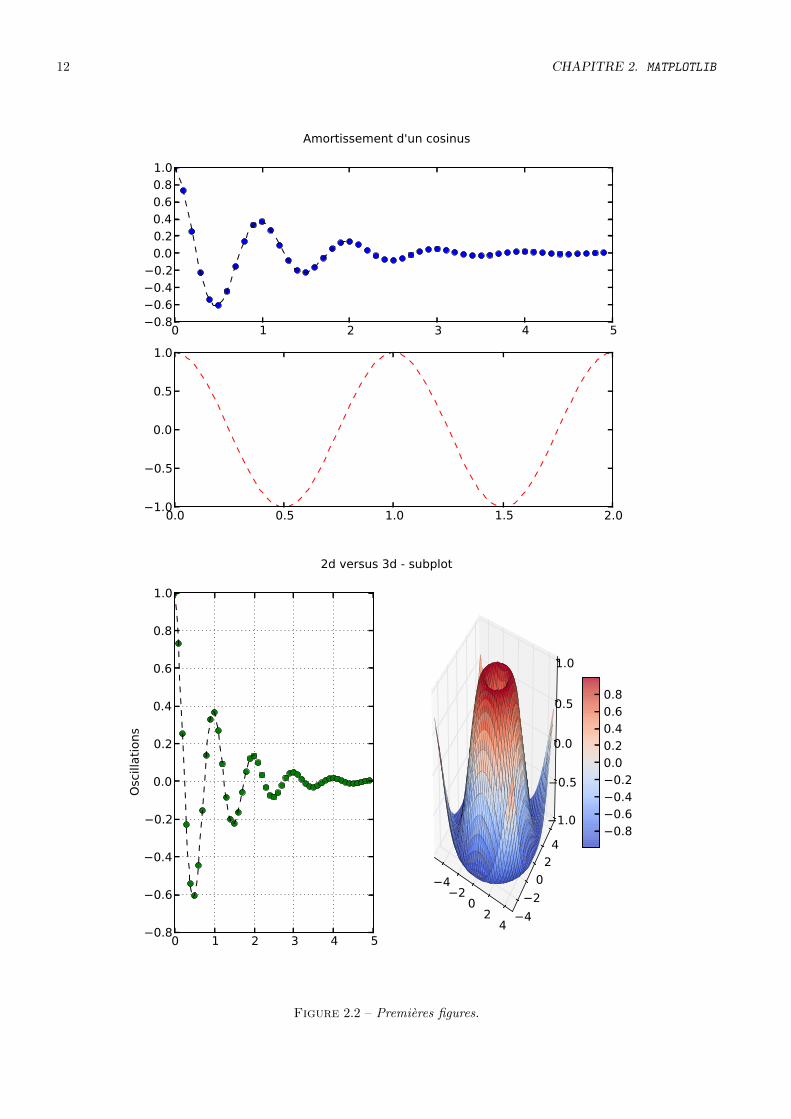
def f(t) :

s1 = np.cos (2*np.pi*t)

e1 = np.exp(-t)

return np.multiply(s1 ,e1)

# vecteurs d’abscisses

t1 = np.arange (0.0, 5.0, 0.1) # pas de 0.1

t2 = np.arange (0.0, 5.0, 0.01) # pas de 0.01

plt.figure (3)

plt.suptitle("Amortissement d’un cosinus")

plt.subplot(2, 1, 1)

plt.plot(t1 , f(t1), ’bo’)

plt.plot(t2 ,f(t2), ’k--’)

plt.subplot(2, 1, 2)

plt.plot(t2 , np.cos(2 * np.pi * t2), ’r--’)

plt.savefig(’fig4_matplotlib.pdf’)

#

# en 3D

fig = plt.figure (4)

fig.suptitle(’2d versus 3d - subplot ’)

#

# premier subplot

ax = fig.add_subplot (1, 2, 1)

l = ax.plot(t1 , f(t1), ’bo’,

t2, f(t2), ’k--’, markerfacecolor=’green ’)

ax.grid(True) # ajout d’une grille

ax.set_ylabel(’Oscillations ’)

#

# second subplot

ax = fig.add_subplot (1, 2, 2, projection=’3d’)

X = np.arange(-5, 5, 0.25)

Y = np.arange(-5, 5, 0.25)

X, Y = np.meshgrid(X, Y)

R = np.sqrt(X**2 + Y**2)

Z = np.sin(R)

from matplotlib import cm

surf = ax.plot_surface(X, Y, Z, rstride=1, cstride=1, cmap=cm.coolwarm ,

linewidth=0, antialiased=False)

I. PREMIERS GRAPHIQUES 11

ax.set_zlim3d (-1,1)

# barre verticale a droire

fig.colorbar(surf , shrink =0.5, aspect =10)

plt.savefig(’fig5_matplotlib.pdf’)

plt.show()

Ceci donne les figures

−π −π/2 0 π/2 π

1

0

1cosinussinus

x axix

43

21

01

23

4

y axix

32

10

12

34

5

z axix

2.0

1.5

1.0

0.5

0.0

0.5

1.0

1.5

2.0

Courbe parametrique

Figure 2.1 – Premieres figures.

12 CHAPITRE 2. MATPLOTLIB

0 1 2 3 4 50.80.60.40.20.00.20.40.60.81.0

0.0 0.5 1.0 1.5 2.01.0

0.5

0.0

0.5

1.0

Amortissement d'un cosinus

0 1 2 3 4 50.8

0.6

0.4

0.2

0.0

0.2

0.4

0.6

0.8

1.0

Osc

illati

ons

42

02

44

2

0

2

4

1.0

0.5

0.0

0.5

1.0

0.80.60.40.2

0.00.20.40.60.8

2d versus 3d - subplot

Figure 2.2 – Premieres figures.

Chapitre 3

SciPy

.1 Algebre lineaire

>>> from scipy import linalg

>>> A = np.random.rand (3,3)

>>> A

array ([[ 0.00102176 , 0.33477738 , 0.79966335] ,

[ 0.03907913 , 0.50905322 , 0.01842479] ,

[ 0.47880221 , 0.89798492 , 0.32825253]])

>>> b = np.random.rand (3,1)

>>> b

array ([[ 0.00188417] ,

[ 0.89028083] ,

[ 0.6127925 ]])

>>> x = linalg.solve(A, b)

>>> x

array ([[ -1.76202966] ,

[ 1.91298333] ,

[ -0.79625883]])

>>> np.dot(A,x) - b

array ([[ 0.00000000e+00],

[ 1.11022302e-16],

[ 0.00000000e+00]])

linalg.det(A) determinant

linalg.inv(A) inverse

U, D, V = linalg.svd(A) decomposition en valeurs singulieres

norm(a[, ord]) norme matricielle ou d’un vecteur

lstsq(a, b[, cond, ...]) Solution aux moindres carres de Ax = b

expm(A[, q]) exponentielle de matrice utilisant approximant depade

Voici un petit exemple de regression lineaire. 1On desire predire la hauteur (en feet) d’un arbre d’une essencedonnee a partir de la connaissance de son diametre a 1m30 (en inches). Pour cela on a collecte les donnees suivantes :

Diametres 2.3 2.5 2.6 3.1 3.4 3.7 3.9 4.0 4.1 4.1Hauteurs 7 8 4 4 6 6 12 8 5 7Diametres 4.2 4.4 4.7 5.1 5.5 5.8 6.2 6.9 6.9 7.3Hauteurs 8 7 9 10 13 7 11 11 16 14

# -*- coding : utf -8 -*-

"""

Created on Sun Apr 21 22 :35 :37 2013

@author : gergaud

1. Donnees provenant de BRUCE et SCHUMACHER Forest mensuration - Mc Graw-Hill book company, ine - 1950 - 3e edition

13

14 CHAPITRE 3. SCIPY

Linear regression example

Donn\’ees provenant de BRUCE\ et SCHUMACHER Forest mensuration - Mc

Graw -Hill book company , ine - 1950 - 3e \’edition}On d\’esire pr\’edire la

hauteur (en feet) d’un arbre d’une essence donn\’ee \‘a partir de la

connaissance de son diam\‘etre \‘a 1m30 (en inches). Pour cela on a

collect\’e les donn\’ees suivantes :

"""

import numpy as np

from scipy import linalg

import matplotlib.pyplot as plt

# Datas

y = np.array([7, 8, 4, 4, 6, 6, 12, 8, 5, 7, 8, 7, 9, 10, 13, 7, 11, 11, 16,

14], dtype=float)

x = np.array ([[2.3 , 2.5, 2.6, 3.1, 3.4, 3.7, 3.9, 4, 4.1, 4.1, 4.2, 4.4, 4.7,

5.1, 5.5, 5.8, 6.2, 6.9, 6.9, 7.3]]).T

n = y.size

print(x.shape ,y.shape , np.ones((n,1)).shape)

X = np.concatenate ((np.ones((n,1)),x) ,1)

print(X)

#beta , res , r, s = linalg.lstsq(X,y)

#print(beta , res , r, s)

beta = linalg.lstsq(X,y) # renvoie une liste avec tous les param etres en

sortie

print(beta [0][0] , beta [0][1])

print("beta = ", beta)

beta2 = linalg.solve(np.dot(X.T,X),np.dot(X.T,y))

print("beta2 = ", beta2)

plt.figure ()

plt.plot(x,y, ’bo’)

xx = np.linspace(min(x),max(x) ,2)

yy = beta [0][0] + beta [0][1]* xx

plt.plot(xx ,yy ,label="rk42")

plt.xlabel(’$x$’)

plt.ylabel(’$y$’)

#plt.legend(loc=’upper left ’)

print(’fin du programme ’)

plt.savefig("fig1_scipy.pdf")

plt.show()

15

2 3 4 5 6 7 8x

4

6

8

10

12

14

16

y

Figure 3.1 – Exemple de regression lineaire.

16 CHAPITRE 3. SCIPY

Bibliographie

[1] Tentative numpy tutorial, document web, 2013. http://www.scipy.org/Tentative_NumPy_Tutorial.

[2] NumPy community. Numpy user guide, release 1.8.0.dev-fd6f038, 2013. http://docs.scipy.org/doc/

numpy-dev/numpy-user.pdf.

[3] Valentin Haenel, Emmanuelle Gouillart, and Gael Varoquaux editors. Python scientific lecture notes, release2013.1. http://scipy-lectures.github.com, 2013.

17