Experiments in Information Storage and

Retrieval Using Mumps

Kevin C. Ó Kane

Second Edition

1

Copyright © 2009, 2010, 2011 by Kevin C. Ó Kane. All rights reserved.

The author may be contacted at:

kc.okane@gmail.com

Department of Computer ScienceThe University of Northern IowaCedar Falls, Iowa 50614-0507

http://www.omahadave.com

Graphics and production design by the

Threadsafe Publishing & Railway Maintenance Co.Hyannis, Nebraska

CreateSpace Publishing

ISBN: EAN:

Revision: 2.01April 10, 2011

2

Table of Contents

1 Introduction............................................................................................7

1.1 What is Information Retrieval?.................................................................................71.2 Additional Resources.............................................................................................12

2 Programming Models and Mumps..........................................................13

2.1 Comparing Mumps for IS&R with Other Approaches .............................................142.2 Hierarchical and Multi-Dimensional Indexing.........................................................16

3 OSU MEDLINE Data Base .......................................................................19

3.1 Original TREC-9 Version.........................................................................................193.2 MEDLINE Style Version...........................................................................................213.3 Compact Stemmed Version ..................................................................................22

4 Basic Hierarchical Indexing Examples.....................................................23

4.1 The Medical Subject Headings (MeSH) ..................................................................234.2 Building a MeSH Structured Global Array...............................................................244.3 Displaying the MeSH Global Array Part I................................................................284.4 Printing the MeSH Global Array Part II...................................................................304.5 Displaying Global Arrays in Key Order...................................................................314.6 Searching the MeSH Global Array..........................................................................334.7 Web Browser Search of the MeSH Global Array.....................................................364.8 Indexing OHSUMED by MeSH Headings.................................................................424.9 MeSH Hierarchy Display of OHSUMED Documents.................................................444.10 Database Compression .......................................................................................454.11 Accessing System Services from Mumps ............................................................46

5 Indexing, Searching and Information Retrieval.......................................48

5.1 Indexing Models.....................................................................................................48

6 Searching.............................................................................................49

6.1 Boolean Searching and Inverted Files....................................................................506.2 Non-Boolean Searching .........................................................................................576.3 Multimedia QUERIES .............................................................................................57

7 Measuring Retrieval System Effectiveness..............................................58

7.1 Precision and Recall...............................................................................................58

8 Document Indexing...............................................................................60

8.1 Overview - The Big Picture.....................................................................................608.2 Vocabularies..........................................................................................................608.3 Basic Dictionary Construction ...............................................................................64

8.3.1 Basic Dictionary of Stemmed Words Using Mumps........................................................648.3.2 Basic Dictionary of Stemmed Words Using Linux System Programs...............................65

8.4 Zipf's Law .............................................................................................................668.5 What are Good Indexing Terms? ...........................................................................68

8.5.1 WordNet ....................................................................................................................... 708.6 Stop Lists ..............................................................................................................72

3

8.6.1 Building a Stop List .......................................................................................................73

9 Vector Space Model ..............................................................................77

9.1 Overview...............................................................................................................779.2 Basic Similarity Functions......................................................................................809.3 Other Similarity Functions ....................................................................................81

10 Document-Term Matrix........................................................................83

10.1 Building a Document-Term Matrix.......................................................................8310.2 Assigning Word Weights .....................................................................................8510.3 Inverse Document Frequency Weight..................................................................89

10.3.1 OSU MEDLINE Data Base IDF Weights .........................................................................8910.3.2 Wikipedia Data Base IDF Weights ...............................................................................9010.3.3 Calculating IDF Weights ..............................................................................................90

10.4 Signal-noise ratio (see Salton83 links, pages 63-66) ...........................................9110.5 Discrimination Coefficients (pages 66-71) and ...................................................91

11 Term-Document Matrix........................................................................97

11.1 Retrieval Using the Doc-Term Matrix ..................................................................9711.2 Retrieval Using the Term-Doc Matrix ..................................................................9811.3 Weighted Scanning the Term-Doc Matrix ............................................................98

12 Scripted Test Runs ...........................................................................100

13 Simple Term Based Retrieval .............................................................108

14 Thesaurus construction .....................................................................114

14.1 Basic Term-Term Co-Occurrence Matrix ...........................................................11514.2 Advanced Term Term Similarity Matrix..............................................................11814.3 Position Specific Term-Term Matrix...................................................................11914.4 Term-Term clustering .......................................................................................12414.5 Construction of Term Phrases............................................................................126

15 Document-Document Matrix...............................................................127

15.1 File and Document Clustering (Salton83, pages 215-222) ................................129

16 Web Page Access - Simple Keyword Based Logical Expression Server Page ................................................................................................................133

17 N-gram encoding ..............................................................................139

18 Indexing Text Features in Genomic Repositories ................................145

18.1 Implementation ................................................................................................14718.2 Data Sets ..........................................................................................................14918.3 Multiple Step Protocol .......................................................................................14918.4 Retrieval ...........................................................................................................15218.5 Results and Discussion .....................................................................................153

19 Overview of Other Methods ...............................................................155

19.1 Using Sort Based Techniques.............................................................................15519.2 Latent Semantic Model .....................................................................................155

4

19.3 Single Term Based Indexing .............................................................................15519.4 Phrase Based Indexing ......................................................................................15519.5 N-Gram Based Indexing ....................................................................................156

20 Visualization ....................................................................................157

21 Applications to Genomic Data Bases ..................................................158

21.1 GenBank ...........................................................................................................15821.2 Alignment Algorithms .......................................................................................15921.3 Case Study: Indexing the "nt" Data Base ..........................................................15921.4 Experiment Design ...........................................................................................16121.5 Results ..............................................................................................................16321.6 Conclusions .......................................................................................................170

22 Miscellaneous Links ..........................................................................171

22.1 Flesch–Kincaid readability test...........................................................................171

23 Configuring a RAID Drive in Linux.......................................................172

24 Configuring Apache and PHP..............................................................173

24.1 Creating a web page in your directory and configuring Apache.........................17324.2 Runing a web based PHP program.....................................................................174

25 File Processing..................................................................................176

25.1 Basic C File Processing Examples......................................................................17625.1.1 Byte-wise File Copy....................................................................................................17625.1.2 Line-wise File Copy....................................................................................................17625.1.3 Open two files and copy one to the other..................................................................176

25.2 64 Bit File Addressing. ......................................................................................17725.2.1 Simple Direct Access Example...................................................................................17825.2.2 MeSH Headings Concordance in C.............................................................................178

25.3 Huffman Coding in Mumps.................................................................................17925.4 Optimum Weight Balanced Binary Tree Algorithm in C......................................18125.5 Optimum Weight Balanced Binary Tree Algorithm in Mumps.............................18425.6 Hu-Tucker Weight Balanced Binary Trees .........................................................18725.7 Self Adjusting Balanced Binary Trees (AVL) ......................................................18725.8 B-Trees .............................................................................................................18725.9 Soundex Coding ................................................................................................19425.10 MD5 - Message Digest Algorithm 5 .................................................................195

26 References........................................................................................196

Index of FiguresFigure 1 DBMS data table...................................................8Figure 2 Two dimensional display of data...........................8Figure 3 Multidimensional display.......................................9Figure 4 Example DNA Sequence......................................10Figure 5 Example BLAST Result........................................10Figure 6 View of Old State House, Boston ........................11Figure 7 Another view of the State House........................12Figure 8 Online resources.................................................12Figure 9 - Global array tree...............................................17Figure 10 - Creating a global array...................................18

Figure 11 Original OSUMED format...................................20Figure 12 OSUMED modified format.................................21Figure 13 Modified OSUMED database..............................22Figure 14 Sample MeSH Hierarchy....................................23Figure 15 Global Array Commands...................................24Figure 16 MeSH Tree.........................................................26Figure 17 MeSH Structured Global Array..........................27Figure 18 Creating the Mesh tree.....................................28Figure 19 Program to print MeSH tree..............................28Figure 20 Printed the Mesh tree........................................30

5

Figure 21 Alternate MeSH tree printing program..............30Figure 22 Alternative MeSH printing output......................31Figure 23 MeSH global array codes...................................32Figure 24 Program to print MeSH global...........................32Figure 25 MeSH global printed..........................................33Figure 26 Program to search MeSH global array..............34Figure 27 MeSH keyword search results...........................36Figure 28 HTML <FORM> example...................................36Figure 29 Web based search program..............................37Figure 30 Browser display of <FORM> tag.......................39Figure 31 Browser display of results.................................40Figure 32 Example <FORM> input types..........................41Figure 33 Browser display of Figure 32.............................41Figure 34 Locate instances of MeSH keywords.................43Figure 35 Titles organized by MeSH code.........................44Figure 36 Hierarchical MeSH concordance program.........44Figure 37 Hierarchical MeSH concordance........................45Figure 38 Dump/Restore example....................................46Figure 39 Invoking system sort from Mumps....................47Figure 40 Overview of Indexing........................................48Figure 41 Inverted search.................................................50Figure 42 STAIRS file organization....................................52Figure 43 Boolean search in Mumps.................................53Figure 44 Boolean search results......................................55Figure 45 1979 Tymnet search.........................................56Figure 46 Precision/recall example...................................58Figure 47 Precision/recall graph........................................59Figure 48 Overview of basic document indexing..............60Figure 49 ACM classification system.................................62Figure 50 List of stemmed terms......................................65Figure 51 Modified dictionary program.............................65Figure 52 Dictionary load program...................................65Figure 53 Dictionary construction using Linux programs 65Figure 54 Reformat.mps...................................................67Figure 55 dictionary.mps..................................................67Figure 56 Zipf's Law example...........................................67Figure 57 Zipf constants - The Dead.................................68Figure 58 Zipf constants - OHSUMED................................68Figure 59 Best indexing terms..........................................69Figure 60 WordNet example.............................................71Figure 61 WordNet example.............................................72Figure 62 Stop list example..............................................73Figure 63 Stop list example..............................................73Figure 64 Frequency of top 75 OSUMED words...............75Figure 65 Frequency of top 75 Wikipedia words ..............76Figure 66 Vector space model..........................................78Figure 67 Vector space queries.........................................78Figure 68 Vector space clustering.....................................79Figure 69 Vector space similarities...................................79Figure 70 Similarity functions...........................................80Figure 71 Example similarity coefficient calculations.......81Figure 72 Basic document-term matrix construction........84Figure 73 Example word weights......................................88Figure 74 IDF calculation...................................................91Figure 75 Modified centroid algorithm..............................94

Figure 76 Enhanced modified centroid algorithm.............96Figure 77 Simple retrieval program..................................98Figure 78 Term-Doc matrix search...................................98Figure 79 Weighted Term-Doc matrix search...................99Figure 80 Example BASH script.......................................108Figure 81 Simple cosine based retrieval.........................112Figure 82 Faster simple retrieval....................................114Figure 83 Term-term matrix............................................116Figure 84 Term-Term correlation matrix.........................117Figure 85 Frequency of term co-occurrences.................118Figure 86 Term-term similarity matrix............................119Figure 87 Proximity Weighted Term-Term Matrix ..........121Figure 88 Proximity Weighted Term-Term Corellations. .123Figure 89 Ranked Proximity Weighted Term-Term

correlations........................................................................123Figure 90 Term-Term clustering......................................125Figure 91 Term Clusters..................................................126Figure 92 Term Cohesion................................................127Figure 93 Term Cohesion Results...................................127Figure 94 Doc-Doc matrix...............................................129Figure 95 Document clustering.......................................130Figure 96 Example Document Document Clustering......131Figure 97 Document hyper-clusters................................133Figure 98 Browser based retrieval..................................135Figure 99 Browser based retrieval..................................136Figure 100 Converting to FASTA Format in Mumps........140Figure 101 Converting to Fasta Format in C...................141Figure 102.......................................................................142Figure 103.......................................................................142Figure 104.......................................................................143Figure 105.......................................................................143Figure 106.......................................................................146Figure 107 Indexing GENBANK........................................151Figure 108.......................................................................153Figure 109.......................................................................161Figure 110 ......................................................................163Figure 111.......................................................................164Figure 112.......................................................................165Figure 113.......................................................................165Figure 114.......................................................................166Figure 115.......................................................................167Figure 116.......................................................................168Figure 117.......................................................................169Figure 118 Example PHP Program..................................175Figure 119 Byte-wise file copy........................................176Figure 120 Line-wise file copy.........................................176Figure 121 File Copy.......................................................177Figure 122.......................................................................178Figure 123 Mesh Concordance in C.................................179Figure 124 Huffman coding in Mumps............................181Figure 125.......................................................................184Figure 126 Optimum binary tree example......................185Figure 127 Mumps Optimal Binary Tree Program...........187Figure 128.......................................................................194

6

1 Introduction

1.1 What is Information Retrieval?

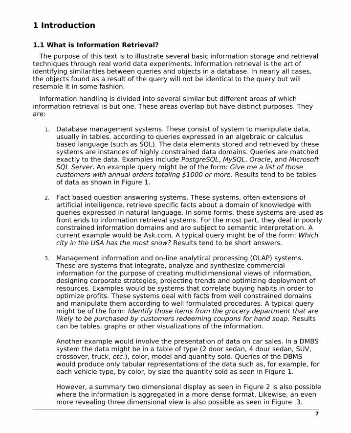
The purpose of this text is to illustrate several basic information storage and retrieval techniques through real world data experiments. Information retrieval is the art of identifying similarities between queries and objects in a database. In nearly all cases, the objects found as a result of the query will not be identical to the query but will resemble it in some fashion.

Information handling is divided into several similar but different areas of which information retrieval is but one. These areas overlap but have distinct purposes. They are:

1. Database management systems. These consist of system to manipulate data, usually in tables, according to queries expressed in an algebraic or calculus based language (such as SQL). The data elements stored and retrieved by these systems are instances of highly constrained data domains. Queries are matched exactly to the data. Examples include PostgreSQL, MySQL, Oracle, and Microsoft SQL Server. An example query might be of the form: Give me a list of those customers with annual orders totaling $1000 or more. Results tend to be tables of data as shown in Figure 1.

2. Fact based question answering systems. These systems, often extensions of artificial intelligence, retrieve specific facts about a domain of knowledge with queries expressed in natural language. In some forms, these systems are used as front ends to information retrieval systems. For the most part, they deal in poorly constrained information domains and are subject to semantic interpretation. A current example would be Ask.com. A typical query might be of the form: Which city in the USA has the most snow? Results tend to be short answers.

3. Management information and on-line analytical processing (OLAP) systems. These are systems that integrate, analyze and synthesize commercial information for the purpose of creating multidimensional views of information, designing corporate strategies, projecting trends and optimizing deployment of resources. Examples would be systems that correlate buying habits in order to optimize profits. These systems deal with facts from well constrained domains and manipulate them according to well formulated procedures. A typical query might be of the form: Identify those items from the grocery department that are likely to be purchased by customers redeeming coupons for hand soap. Results can be tables, graphs or other visualizations of the information.

Another example would involve the presentation of data on car sales. In a DMBS system the data might be in a table of type (2 door sedan, 4 dour sedan, SUV, crossover, truck, etc.), color, model and quantity sold. Queries of the DBMS would produce only tabular representations of the data such as, for example, for each vehicle type, by color, by size the quantity sold as seen in Figure 1.

However, a summary two dimensional display as seen in Figure 2 is also possible where the information is aggregated in a more dense format. Likewise, an even more revealing three dimensional view is also possible as seen in Figure 3.

7

model type color quantity

Buick 2 DR red 3

Buick convertible blue 5

Buick SUV white 4

Toyota 4 DR silver 6

Toyota truck black 10

Toyota truck blue 5

Toyota SUV red 3

Ford truck black 6

Ford truck gray 4

Ford 4 DR green 4

Ford SUV yellow 3

Ford 2 DR silver 3

Ford 2 DR black 5

Honda SUV red 3

Honda van gray 5

Honda van blue 3

Honda van white 5

Figure 1 DBMS data table

Model

Colorred white blue black gray yellow silver

Buick 3 4 5 0 0 0 0

Toyota 3 0 5 10 0 0 0

Ford 0 0 0 5 4 3 3

Honda 3 5 3 0 5 0 0

Totals 9 9 8 15 9 3 3

Figure 2 Two dimensional display of data

8

Figure 3 Multidimensional display

4. Information retrieval systems. These systems retrieve natural language text documents using natural language queries. The matching process is approximate and subject to semantic interpretation. A typical query might be of the form: Give me articles concerning nuclear physics that concern nuclear reactor construction. Results are titles, abstracts and locator information to original articles, books or web pages.

For example, a query to an information retrieval system might be of the form: give me articles about aviation and the results might include articles about early pioneers in the field, technical reports on aircraft design, flight schedules on airlines, information on airports and so on. For example, the term aviation when typed into Google results in about 111,000,000 hits all of which have something to do with aviation.

Another aspect to information retrieval is its relationship with the user. The articles retrieved in response to a query from a grade school student will be significantly different than those returned for a graduate student. This would not be the case in any of the other systems listed above: the city with the most snow does not depend on the educational level of the questioner.

An information retrieval system also involves relevance feedback where by the system interacts with the user in order to refine the query and the resulting answer. Some systems learn from their users and respond accordingly.

9

Information retrieval isn't restricted to text retrieval. So, if you have a cut of a musical piece such as from the Beethoven 9th Symphony and you want to find other music similar to it such as from the Beethoven Choral Fantasy, you need a retrieval engine that can detect the obvious similarities, but not match a chorus from von Weber's der Freischutz.

Similar examples exist in many other areas. In Bioinformatics, researchers often identify DNA or protein sequences and search massive databases for similar (and sometimes only distantly related) sequences. For example, see the the DNA sequence in Figure 4.

>gi|2695846|emb|Y13255.1|ABY13255 Acipenser baeri mRNA for immunoglobulin heavy chain, TGGTTACAACACTTTCTTCTTTCAATAACCACAATACTGCAGTACAATGGGGATTTTAACAGCTCTCTGTATAATAATGACAGCTCTATCAAGTGTCCGGTCTGATGTAGTGTTGACTGAGTCCGGACCAGCAGTTATAAAGCCTGGAGAGTCCCATAAACTGTCCTGTAAAGCCTCTGGATTCACATTCAGCAGCGCCTACATGAGCTGGGTTCGACAAGCTCCTGGAAAGGGTCTGGAATGGGTGGCTTATATTTACTCAGGTGGTAGTAGTACATACTATGCCCAGTCTGTCCAGGGAAGATTCGCCATCTCCAGAGACGATTCCAACAGCATGCTGTATTTACAAATGAACAGCCTGAAGACTGAAGACACTGCCGTGTATTACTGTGCTCGGGGCGGGCTGGGGTGGTCCCTTGACTACTGGGGGAAAGGCACAATGATCACCGTAACTTCTGCTACGCCATCACCACCGACAGTGTTTCCGCTTATGGAGTCATGTTGTTTGAGCGATATCTCGGGTCCTGTTGCTACGGGCTGCTTAGCAACCGGATTCTGCCTACCCCCGCGACCTTCTCGTGGACTGATCAATCTGGAAAAGCTTTT

Figure 4 Example DNA Sequence

Where the first line identifies the name and library accession numbers of the sequence and the subsequent lines are the DNA nucleotide codes (the letters A, C, G, and T represent Adenine, Cytosine, Guanine, and Thymine, respectively). A program known as BLAST (Basic Local Alignment Sequencing Tool) can be used to find similar sequences in the online databases of known sequences. If you submit the above to NCBI BLAST (National Center for Biotechnology Information), they will conduct a search of their nr database of 6,284,619 nucleotide sequences, presently more than 22,427,755,047 bytes in length. The result is a ranked list of hits of sequences in the data base based on their similarity to the query sequence. Sequences found whose similarity score exceeds a threshold are displayed. One of these is shown in Figure 5.

>gb|U17058.1|LOU17058 Lepisosteus osseus Ig heavy chain V region mRNA, partial cds

Score = 151 bits (76), Expect = 4e-33 Identities = 133/152 (87%), Gaps = 0/152 (0%) Strand=Plus/Plus

Query 242 TGGGTGGCTTATATTTACTCAGGTGGTAGTAGTACATACTATGCCCAGTCTGTCCAGGGA 301 |||||||| ||||||||| | | ||| || | |||||||||| |||||||||||||||||Sbjct 4 TGGGTGGCGTATATTTACACCGATGGGAGCAATACATACTATTCCCAGTCTGTCCAGGGA 63

Query 302 AGATTCGCCATCTCCAGAGACGATTCCAACAGCATGCTGTATTTACAAATGAACAGCCTG 361 |||||| |||||||||||||| ||||||| | |||||| ||||| |||| |||||||Sbjct 64 AGATTCACCATCTCCAGAGACAATTCCAAGAATCAGCTGTACTTACAGATGAGCAGCCTG 123

Query 362 AAGACTGAAGACACTGCCGTGTATTACTGTGC 393 ||||||||||||||||| ||||||||||||||Sbjct 124 AAGACTGAAGACACTGCTGTGTATTACTGTGC 155

Figure 5 Example BLAST Result

In the display from BLAST seen in Figure 5, the sections of the query sequence that match a portion of a sequence in the database are shown. The numbers at the beginning and ends of the lines are the starting and ending points of the subsequence

10

(relative to one, the start of all sequences). Where there are vertical lines between the query and the subject, there is an exact match. Where there are blanks, there was a mismatch.

It should be clear that, even though the subject is different than the query in many places, the two have a high degree of similarity.

Also, consider the search for similar images. Again, this involves searching for similarities, not identity. For example, a human observer would clearly see the pictures in Figures 6 and 7 in the figures as dealing with the same subject, despite the differences. An obvious question would be, can you write a computer program to see the obvious similarity?

Figure 6 View of Old State House, Boston

11

Figure 7 Another view of the State House

1.2 Additional Resources

The following is a list of links to some other books on information storage and retrieval that are available on the Internet

1. INFORMATION RETRIEVAL by C. J. van RIJSBERGEN

http://www.dcs.gla.ac.uk/Keith/Preface.html

2. Introduction to Information Retrieval, by Christopher D. Manning, Prabhakar Raghavan and Hinrich Schütze

http://nlp.stanford.edu/IR-book/information-retrieval-book.html

3. Modern Information Retrieval, Chapter 10: User Interfaces and Visualization - by Marti Hearst

http://www.sims.berkeley.edu/~hearst/irbook/10/chap10.html

Figure 8 Online resources

12

2 Programming Models and Mumps

In this text we will conduct experiments illustrating several approaches to indexing and retrieving information from very large text data sets. These will require very large files and substantial amounts of computer time.

Many of the basic programming models in IS&R make use of large, disk resident, sparse, string indexed, multi-dimensional matrices. For the most part, data structures such as these are not well supported, if at all, in most programming languages.

Rather than implement the models from scratch in C/C++, Java or PHP, in this text we will use the Mumps language. Mumps is a very simple interpretive scripting language that easily supports the disk based data structures needed for our purposes and it can be learned in a matter of hours.

Mumps (also referred to as 'M') is a general purpose programming language that supports a native hierarchical and multi-dimensional data base facility. It is supported by a large user community (mainly biomedical), and a diversified installed application software base. The language originated in the mid-60's at the Massachusetts General Hospital and it became widely used in both clinical and commercial settings.

As originally conceived, Mumps differed from other mini-computer based languages of the late 1960's by providing: 1) an easily manipulated hierarchical (multi-dimensional) data base that was well suited to representing medical records; 2) flexible string handling support; and (3) multiple concurrent tasks in limited memory on very small machines. Syntactically, Mumps is based on an earlier language named JOSS and has an appearance that is similar to early versions of BASIC that were also based on JOSS.

There are two commercial implementations of Mumps. these are:

1. InterSystems' Caché. Intersystems has made many extensions to their product and now refer to it under the name Caché. A single user Windows version is available for individual use. See:

http://www.intersystems.com/cache/

2. Fidelity National Information Systems GT.M. GT.M is available under the GPL License for both Linux and Windows. See:

http://fisglobal.com/Products/TechnologyPlatforms/GTM/index.htm

A non-commercial, open source, GPL licensed version is available from this author. It has also been extended to include many functions useful in IS&R experiments. See:

http://www.cs.uni.edu/~okane/source/MUMPS-MDH/

for the latest distribution and installation instructions.

This version of Mumps is available both as an interpreter which directly executes Mumps source programs and as a compiler which translates the Mumps source code to C++ and then compiles the result to executable binaries. These notes will assume you

13

are using the interpreter which is generally easier to use unless you are experienced in dealing with C++ error messages. The performance differences are negligible since most of our use will be disk I/O based and both versions use the same disk server code.

You should consult the companion text The Mumps Programming Language for details on the Mumps language. This is available as a free PDF file for students or for purchase in printed form at:

http://www.amazon.com

2.1 Comparing Mumps for IS&R with Other Approaches

In order to evaluate different programming approaches to IS&R experiments, several years ago a basic automatic indexing experiment along the lines of that given in Chapter 9 of Salton (Salton 1989) was implemented in Mumps and compared to other methodologies.

Salton's approach makes heavy usage of vectors and matrices to store documents, terms, text, queries and intermediate results. From these experiments we were able to assess the viability of Mumps in terms of ease of use, speed, storage requirements, programmer productivity, and suitability to the programming problems at hand. The details are given below.

When working with a document collection of any meaningful scope, vectors, matrices and file structures can quickly grow to enormous size. The information retrieval system was tested using a corpus of documents concerning computer science subjects. Each document consisted of a title, reference information, and an abstract averaging approximately 15 lines in length.

In the test, there were 5,614 documents with 132,502 word occurrences of which, not counting stop list words, 7,812 words were unique with an average frequency of use per word of approximately 15.

In the Salton model, each document is a vector consisting of the words in the document and the frequency of occurrence of each word.

Taking all the document vectors together, the collection is viewed as a two-dimensional matrix where the rows are identified by document number and the columns are identified by the words or terms from the vocabulary. Each element in the matrix gives the number of times the word occurred in a document. This is called a document-term matrix.

Thus, the document-term matrix for this collection was 5,614 rows by 7,812 columns for a total number of elements of 43,856,568. A related matrix used in this model, derived from the document-term matrix, is called the term-term matrix, had in excess of 61 million elements in this example.

Representing data structures of this size while providing fast, efficient, direct access to any value stored at any element is of critical importance to the Salton matrix based model. Ideally, an implementation language will provide a transparent means by which the conceptual model can be realized through indexed access to elements of the

14

matrices by character string keyword rather than by numeric subscript as is typically the case in most languages. Furthermore, the extent and number of array dimensions must be dynamically settable.

In a typical document-term matrix, many elements have values of zero. This happens when a term does not occur in a particular document. In this experiment, the average number of terms per document was approximately 15. Thus, nearly 7,800 possible positions per row were zero (non-existent) in a typical case.

In order to quickly access rows of data when stored on disk, the locations of the rows

should be predictable. That is, the rows should be of fixed length thus allowing a disk access method to access the vector for any document by multiplying the document number by the row size and thus calculating an offset relative to the start of the file where the record is located. There are several possible ways to do this:

1. Coded Tuples

One approach is to represent each row (document) as a collection of tuples each of which consists of a token and a frequency. The token identifies the term and the frequency gives the weight of the term in the document. In this scheme, a minimum of four bytes would be required for each tuple (2 bytes to represent a number identifying the term and two bytes to represent the frequency). In order for the file to be easily accessed, each row must be a fixed length record. Allowing for 100 terms per row, a worst case estimate, this required a 2,245,600 byte file to represent the test collection (5614*100*4).

2. Bit Maps Alternatively, a bit mapping model represents documents as positional binary vectors with a "1" indicating that a given term occurs in a document and a "0" indicating that it does not. While this is done to conserve space and improve vector access time, it also precludes the storage of information concerning the relative weight or strength of the term in a document. Using the test data set, a positional binary vector representation of each document would be 977 bytes in length for a total of 5,484,878 bytes for the collection as a whole.

3. SQL

A row-wise vector representation in which each term was represented by a numeric frequency count of two bytes would required 15,624 bytes per document (row) or 87,713,136 bytes to represent the entire collection.

4. Mumps Global Arrays

The Mumps Global array model stores only elements that exist along with indexing information. There were 83,895 non-zero elements in the experimental document-term matrix. Each element consisted of a frequency which, including overhead, required approximately 21 bytes for a total storage requirement or approximately 1,761,795 bytes for the collection as a whole.

15

As can be seen, the Mumps approach results in a substantial reduction in overall storage requirements and, consequently, faster file access. It also makes it possible to reasonably consider very large document collections using the Salton vector space model.

2.2 Hierarchical and Multi-Dimensional Indexing

In the following sections are examples of Mumps programs used to store and manipulate basic hierarchical indexing and multi-dimensional structures. While table based Relational Database Management Systems (RDBMS) such as IBM DB2, MySQL, Microsoft SQL Server, PostgreSQL, Oracle RDBMS, dominate the commercial realm, not all data models are well suited to a tabular approach. Dynamically organized hierarchically organized data with varying tree path lengths are not well suited for the relational model.

In recent years the term NoSQL has come into use. Generally, it is used to collectively refer to several database designs not organized according to the relational model. In addition to Mumps, some other example implementations include Google's BigTable, Amazon's Dynamo and Apache Cassandra. Some notable users of NoSQL implementations include include Digg (3 TB of data), Facebook (50+ TB of data), and eBay (2 PB of data).

The hierarchical/multi-dimensional approach used in Mumps is also found in IBM IMS was also originally developed in the 1960s and still widely used to this day. IMS is reputed to be IBM's highest revenue software product.

In Mumps and similar systems, the data organization can be viewed either as a tree with varying length paths from the root to an ultimate leaf node or a multi-dimensional sparse matrix.

In Mumps, persistent data, that is, data that can be accessed after the program which created it terminates, is stored in global arrays. Global arrays are disk resident and are characterized by the following:

• They are not declared or pre-dimensioned. • The indices of an array are specified as a comma separated list of numbers or

strings.• Arrays are sparse. That is, if you create an element of an array, let us say

element 10, it does not mean that Mumps has created any other elements. In other words, it does not imply that there exist elements 1 through 9. You must explicitly create these it you want them.

• Array indices may be positive or negative numbers or character strings or a combination of both.

• Arrays may have multiple dimensions limited by the maximum line length (nominally 512 characters but most implementations permit longer lengths).

• Arrays may be viewed as either arrays or trees. • When viewed as trees, each successive index is part of the path description from

the root to a node.• Data may be stored at any node along the path of a tree.• Global array names are prefixed with the up-arrow character (^).

16

For example, consider an array reference of the form ^root("p2","m2","d2"). This could be interpreted to represent a cell in a three dimensional matrix ^root indexed by the values ("p2","m2","d2") or, alternatively, it could be interpreted as a path from the origin (^root) to a final (although not necessarily terminal) node d2.

In either the array or tree interpretation, values may be stored not only at an end node, but also at intermediate nodes. That is, in the example above, data values may be stored at nodes ^root, ^root("p2"), ^root("p2","m2") as well as ^root("p2","m2","d2").

Because Mumps arrays can have many dimensions (limited by implementation defined maximum line length), when viewed as trees, they can be of many levels of depth and these levels may differ in depth from one sub tree to another.

In Mumps, arrays can be accessed directly by means of a set of valid index vales or by navigation of a global array tree primarily by means of the builtin functions $data() and $order(). The first of these, $data(), reports if a node exists, if it has data and if it has descendants. The second, $order(), is used to navigate from one sibling node to the next (or prior) at a given level of a tree.

In the example shown in Figure 9, each successive index added to the description leads to a new node in the tree. Some branches go deeper than others. Some nodes may have data stored at them, some have no data. The $data() function, described in detail below, can be used to determine if a node has data and if it has descendants.

Figure 9 - Global array tree

In the example in Figure 9, only numeric indices were used to conserve space. In fact, however, the indices of global arrays are often character strings.

In a global array tree, the order in which siblings appear in the tree is determined by the collating sequence, usually ASCII. That is, the index with the lowest overall collating sequence value is first branch and the index with the highest value is last branch. The $order() function, described below, can be used to navigate from one sibling to the next at any given level of the tree. The tree from Figure 9 can be created with the code shown Figure 10.

17

1 set ^root(1,37)=12 set ^root(1,92,77)=23 set ^root(1,92,177)=34 set ^root(5)=45 set ^root(8,1)=56 set ^root(8,100)=67 set ^root(15)=78 set ^root(32,5)=89 set ^root(32,5,3)=910 set ^root(32,5,8)=1011 set ^root(32,123)=11

Figure 10 - Creating a global array

In this construction (others are possible), note that several nodes exist but have no data stored. For example, the nodes ^root(1), ^root(8) and ^root(32) exist because they have descendants but they have no data stored at them. On the other hand, the node ^root(32,5) exists, has data and has descendants.

The following examples illustrate using the Mumps hierarchical global array facility to represent tree structured indexing data.

18

3 OSU MEDLINE Data Base

3.1 Original TREC-9 Version

The corpus of text which will be used in many of subsequent examples and experiments is the OSU MEDLINE Data Base which was obtained from the TREC-9 conference. TREC (Text REtrieval Conferences) are annual events sponsored by the National Institute for Standards and Technology (NIST). These data sets are at:

http://trec.nist.gov/data.html

http://trec.nist.gov/data/t9_filtering.html

The original OHSUMED data sets can be found here:

http://ir.ohsu.edu/ohsumed/

The TREC-9 Filtering Track data base consisted of a collection of medically related titles and abstracts:

"... The OHSUMED test collection is a set of 348,566 references from MEDLINE, the on-line medical information database, consisting of titles and/or abstracts from 270 medical journals over a five-year period (1987-1991). The available fields are title, abstract, MeSH indexing terms, author, source, and publication type. The National Library of Medicine has agreed to make the MEDLINE references in the test database available for experimentation, restricted to the following conditions:

1. The data will not be used in any non-experimental clinical, library, or other setting.

2. Any human users of the data will explicitly be told that the data is incomplete and out-of-date.

The OHSUMED document collection was obtained by William Hersh (hersh@OHSU.EDU) and colleagues for the experiments described in the papers below:

Hersh WR, Buckley C, Leone TJ, Hickam DH, OHSUMED: An interactive retrieval evaluation and new large test collection for research, Proceedings of the 17th Annual ACM SIGIR Conference, 1994, 192-201.

Hersh WR, Hickam DH, Use of a multi-application computer workstation in a clinical setting, Bulletin of the Medical Library Association, 1994, 82: 382-389. ..."

The OHSUMED test collection is a set of 348,566 references from MEDLINE, the on-line medical information database, consisting of titles and/or abstracts from 270 medical journals over a five-year period (1987-1991). The data base was filtered and reformatted to conform to the style similar to that used by online NLM MEDLINE abstracts. A compressed, filtered copy of the reformatted data base is here:

http://www.cs.uni.edu/~okane/source/ISR/osu-medline.gz

19

Data from the OHSUMED file were modified and edited into a format similar to that currently used by MEDLINE (see http://www.ncbi.nlm.nih.gov/sites/entrez) in order to present a more easily managed file. The original format used many very long lines which were inconvenient to manipulate as well as a number of fields that were not of interest for this study. A sample of the original file is given in Figure 11 and the revised data base format is shown in Figure 12.

.I 54711

.U 88000001 .S Alcohol Alcohol 8801; 22(2):103-12 .M Acetaldehyde/*ME; Buffers; Catalysis; HEPES/PD; Nuclear Magnetic Resonance; Phosphates/*PD; Protein Binding; Ribonuclease, Pancreatic /AI/*ME; Support, U.S. Gov't, Non-P.H.S.; Support, U.S. Gov't, P.H.S.. .T The binding of acetaldehyde to the active site of ribonuclease: alterations in catalytic activity and effects of phosphate. .P JOURNAL ARTICLE. .W Ribonuclease A was reacted with [1-13C,1,2-14C]acetaldehyde and sodium cyanoborohydride in the presence or absence of 0.2 M phosphate . After several hours of incubation at 4 degrees C (pH 7.4) stable acetaldehyde-RNase adducts were formed, and the extent of their fo rmation was similar regardless of the presence of phosphate. Although the total amount of covalent binding was comparable in the abse nce or presence of phosphate, this active site ligand prevented the inhibition of enzymatic activity seen in its absence. This protec tive action of phosphate diminished with progressive ethylation of RNase, indicating that the reversible association of phosphate wit h the active site lysyl residue was overcome by the irreversible process of reductive ethylation. Modified RNase was analysed using 1 3C proton decoupled NMR spectroscopy. Peaks arising from the covalent binding of enriched acetaldehyde to free amino groups in the ab sence of phosphate were as follows: NH2-terminal alpha amino group, 47.3 ppm; bulk ethylation at epsilon amino groups of nonessential lysyl residues, 43.0 ppm; and the epsilon amino group of lysine-41 at the active site, 47.4 ppm. In the spectrum of RNase ethylated in the presence of phosphate, the peak at 47.4 ppm was absent. When RNase was selectively premethylated in the presence of phosphate, to block all but the active site lysyl residues and then ethylated in its absence, the signal at 43.0 ppm was greatly diminished, an d that arising from the active site lysyl residue at 47.4 ppm was enhanced. These results indicate that phosphate specifically protec ted the active site lysine from reaction with acetaldehyde, and that modification of this lysine by acetaldehyde adduct formation res ulted in inhibition of catalytic activity. .A Mauch TJ; Tuma DJ; Sorrell MF.

Figure 11 Original OSUMED format

In Figure 11 the identifier codes mean:

1. .I sequential identifier 2. .U MEDLINE identifier (UI) 3. .M Human-assigned MeSH terms (MH) 4. .T Title (TI) 5. .P Publication type (PT) 6. .W Abstract (AB) 7. .A Author (AU) 8. .S Source (SO)

20

3.2 MEDLINE Style Version

STAT- MEDLINEMH Acetaldehyde/*MEMH BuffersMH CatalysisMH HEPES/PDMH Nuclear Magnetic ResonanceMH Phosphates/*PDMH Protein BindingMH Ribonuclease, Pancreatic/AI/*MEMH Support, U.S. Gov't, Non-P.H.S.MH Support, U.S. Gov't, P.H.S.TI The binding of acetaldehyde to the active site of ribonuclease: ...AB Ribonuclease A was reacted with [1-13C,1,2-14C]acetaldehyde ... of 0.2 M phosphate. After several hours of incubation at 4 degrees C (pH 7.4) stable acetaldehyde-RNase adducts were formed, and the extent of their formation was similar regardless of the presence of phosphate. Although the total amount of covalent binding was comparable in the absence or presence of phosphate, this active site ligand prevented the inhibition of enzymatic activity seen in its absence. This protective action of phosphate diminished with progressive ethylation of RNase, indicating that the reversible association of phosphate with the active site lysyl residue was overcome by the irreversible process of reductive ethylation. Modified RNase was analysed using 13C proton decoupled NMR spectroscopy. Peaks arising from the covalent binding of enriched acetaldehyde to free amino groups in the absence of phosphate were as follows: NH2-terminal alpha amino group, 47.3 ppm; bulk ethylation at epsilon amino groups of nonessential lysyl residues, 43.0 ppm; and the epsilon amino group of lysine-41 at the active site, 47.4 ppm. In the spectrum of RNase ethylated in the presence of phosphate, the peak at 47.4 ppm was absent. When RNase was selectively premethylated in the presence of phosphate, to block all but the active site lysyl residues and then ethylated in its absence, the signal at 43.0 ppm was greatly diminished, and that arising from the active site lysyl residue at 47.4 ppm was enhanced. These results indicate that phosphate specifically protected the active site lysine from reaction with acetaldehyde, and that modification of this lysine by acetaldehyde adduct formation resulted in inhibition of catalytic activity.

(Note: long lines truncated from the above)

Figure 12 OSUMED modified format

In Figure 12:

1. MH means MeSH heading term2. TI means title3. AB means abstract.4. All data fields begin in column 7 and all descriptors begin in column 15. Each entry begins with the text STAT- MEDLINE

This file is referred to as ose.medline in the text below.

21

3.3 Compact Stemmed Version

Additionally, another modified version of the basic OSU MEDLINE file, referred to as below, was constructed from the title and abstract portions of the OHSUMED file which can be found here:

http://www.cs.uni.edu/~okane/source/ISR/medline.translated.txt.gz.

In this file:

1. each document is on one line; 2. each line begins with the marker token xxxxx115xxxxx 3. following the beginning token and separated by on blank is the offset in bytes of

the start of the abstract entry in the long form of the file shown above; 4. next follows, separated by a blank, the document number;

the remainder of the line are the words of the document processed according to: 4.1. words shorter than 3 or longer than 25 letters are deleted;

all words are reduced to lower case;all non-alphanumeric punctuation is removed;

4.2. the words have been processed by a basic stemming procedure leaving only the the word roots;

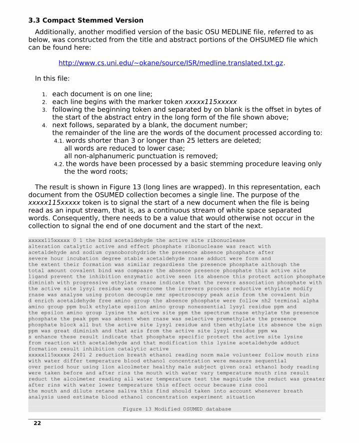
The result is shown in Figure 13 (long lines are wrapped). In this representation, each document from the OSUMED collection becomes a single line. The purpose of the xxxxx115xxxxx token is to signal the start of a new document when the file is being read as an input stream, that is, as a continuous stream of white space separated words. Consequently, there needs to be a value that would otherwise not occur in the collection to signal the end of one document and the start of the next.

xxxxx115xxxxx 0 1 the bind acetaldehyde the active site ribonuclease alteration catalytic active and effect phosphate ribonuclease was react with acetaldehyde and sodium cyanoborohydride the presence absence phosphate after severe hour incubation degree stable acetaldehyde rnase adduct were form and the extent their formation was similar regardless the presence phosphate although the total amount covalent bind was compaare the absence presence phosphate this active site ligand prevent the inhibition enzymatic active seen its absence this protect action phosphate diminish with progressive ethylate rnase indicate that the revers association phosphate with the active site lysyl residue was overcome the irrevers process reductive ethylate modify rnase was analyse using proton decouple nmr spectroscopy peak aris from the covalent bind enrich acetaldehyde free amino group the absence phosphate were follow nh2 terminal alpha amino group ppm bulk ethylate epsilon amino group nonessential lysyl residue ppm and the epsilon amino group lysine the active site ppm the spectrum rnase ethylate the presence phosphate the peak ppm was absent when rnase was selective premethylate the presence phosphate block all but the active site lysyl residue and then ethylate its absence the sign ppm was great diminish and that aris from the active site lysyl residue ppm was enhance these result indicate that phosphate specific protect the active site lysine from reaction with acetaldehyde and that modification this lysine acetaldehyde adduct formation result inhibition catalytic active xxxxx115xxxxx 2401 2 reduction breath ethanol reading norm male volunteer follow mouth rins with water differ temperature blood ethanol concentration were measure sequential over period hour using lion alcolmeter healthy male subject given oral ethanol body reading were taken before and after rins the mouth with water vary temperature mouth rins result reduct the alcolmeter reading all water temperature test the magnitude the reduct was greater after rins with water lower temperature this effect occur because rins cool the mouth and dilute retane saliva this find should taken into account whenever breath analysis used estimate blood ethanol concentration experiment situation

Figure 13 Modified OSUMED database

22

4 Basic Hierarchical Indexing Examples

Hierarchical indexing schemes such as MeSH (Medical Subject Headings), the Library of Congress Classification system, the ACM's Computing Classification System, the Open Directory Project, and many others are widely used to organize and access information. Thus, we begin with some techniques to manipulate hierarchies.

4.1 The Medical Subject Headings (MeSH)

MeSH (Medical Subject Headings) is a hierarchical indexing and classification system developed by the National Library of Medicine (NLM). The MeSH codes are used to code medical records and literature as part of an ongoing research project at the NLM.

The following examples make use of the 2003 MeSH Tree Hierarchy. Newer versions, essentially similar to these, are available from NLM.

Note (required warning): for clinical purposes, this copy of the MeSH hierarchy is out of date and should not be used for clinical decision making. It is used here purely as an example to illustrate a hierarchical index.

A compressed copy of the 2003 MeSH codes is available at:

http://www.cs.uni.edu/~okane/source/ISR/mtrees2003.gz

and also, in text format, at:

http://www.cs.uni.edu/~okane/source/ISR/mtrees2003.html

The 2003 MeSH file consists of nearly 40,000 entries. Each line consists of text and codes which place the text into a hierarchical context. Figure 14 contains a sample from the 2003 MeSH file.

Body Regions;A01Abdomen;A01.047Abdominal Cavity;A01.047.025Peritoneum;A01.047.025.600Douglas' Pouch;A01.047.025.600.225Mesentery;A01.047.025.600.451Mesocolon;A01.047.025.600.451.535Omentum;A01.047.025.600.573Peritoneal Cavity;A01.047.025.600.678Retroperitoneal Space;A01.047.025.750Abdominal Wall;A01.047.050Groin;A01.047.365Inguinal Canal;A01.047.412Umbilicus;A01.047.849Back;A01.176Lumbosacral Region;A01.176.519Sacrococcygeal Region;A01.176.780Breast;A01.236Nipples;A01.236.500Extremities;A01.378Amputation Stumps;A01.378.100

Figure 14 Sample MeSH Hierarchy

The format of the MeSH table is:

23

1. a short text description2. a semi-colon, and 3. a sequence of decimal point separated codes.

Each entry in a code sequence identifies a node in the hierarchy. Thus, in the above, Body Regions has code A01, the Abdomen is A01.047, the Peritoneum is A01.047.025.600 and so forth.

Entries with a single code represent the highest level nodes whereas multiple codes represent lower levels in the tree. For example, Body Regions consists of several parts, one of which is the Abdomen. Similarly, the Abdomen is divided into parts one of which is the Abdominal Cavity. Likewise, the Peritoneum is part of the Abdominal Cavity. An example of the tree structure thus defined can be seen in Figure 16.

The MeSH codes are an example of a controlled vocabulary. That is, a collection of indexing terms that are preselected, defined and authorized by an authoritative source.

4.2 Building a MeSH Structured Global Array

First, our goal here is to write a program to build a global array tree whose structure corresponds to the MeSH hierarchy. In this tree, each successive index in the global array reference will be a successive code from an entry in the 2003 MeSH hierarchy. The text part of each MeSH entry will be stored as the global array data value at both terminal and intermediate indexing levels.

To do this, we want to run a program consisting of Mumps assignment statements similar to the fragment shown in Figure 15. In this example, the code identifiers from the MeSH hierarchy become global array indices and the corresponding text becomes assigned values.

set ^mesh("A01")="Body Regions"set ^mesh("A01","047")="Abdomen"set ^mesh("A01","047","025")="Abdomenal Cavity"set ^mesh("A01","047","025","600")="Peritoneum"...set ^mesh("A01","047","365")="Groin"...

Figure 15 Global Array Commands

A graphical representation of this can be seen in Figure 16 which depicts the MeSH tree and the corresponding Mumps assignment statements needed to create the structured global array corresponding to the diagram.

A program to build a MeSH tree is shown in Figure 17. However, rather than being a program consisting of several thousand Mumps assignment statements, instead we use the Mumps indirection facility to write a short Mumps program that reads the MeSH file and dynamically generates and executes several thousand assignment statements.

24

The program in Figure 17, in a loop (lines 5 through 35), reads a line from the file mesh2003.txt (line 7). On lines 9 and 10 the part of the MeSH entry prior and following the semi-colon are extracted into the strings key and code, respectively. The loop on lines 13 through 15 extracts each decimal point separated element of the code into successively numbered elements of the local array x. On line 19 a string is assigned to the variable z which will be the initial portion of the global array reference to be constructed.

On line 26 elements of the array x are concatenated onto z with encompassing quotes and separating commas. On line 27 the final element of array x is added along with a closing parenthesis, an assignment operator and the value of key and the text is prepended with a Mumps set command. Now the contents of z look like a Mumps assignment statement which is executed on line 35 thus creating the entry in the database. The xecute command in Mumps causes the string passed to it to be treated and executed as Mumps code.

Note that to embed a double-quote character (") into a string, you place two immediately adjacent double-quote characters into the string. Thus: """" means a string of length one containing a double-quote character.

Line 11 uses the OR operator (!) to test if either key or code is the empty string. Note that parentheses are needed in this predicate since expressions in Mumps are executed left-to-right without precedence. Without parentheses, the predicate would evaluate as if it had been written as :

(((key="")!code)="")

which would yield a completely different result!

Line 26 uses the concatenation operator (_) on the local array x(j). Local arrays should be used as little as possible as access to them through the Mumps run-time symbol table which can be slow especially if there are a large number of variables or array elements in the current program.

25

Figure 16 MeSH Tree

26

1 #!/usr/bin/mumps2 # mtree.mps January 13, 20083 4 open 1:"mtrees2003.txt,old"5 for do6 . use 17 . read a8 . if '$test break9 . set key=$piece(a,";",1) // text description10 . set code=$piece(a,";",2) // everything else11 . if key=""!(code="") break12 13 . for i=1:1 do14 .. set x(i)=$piece(code,".",i) // extract code numbers15 .. if x(i)="" break16 17 . set i=i-118 . use 519 . set z="^mesh(" // begin building a global reference20 21 #-----------------------------------------------------------------------22 # build a reference like ^mesh("A01","047","025","600)23 # by concatenating quotes, codes, quotes, and commas onto z24 #-----------------------------------------------------------------------25 26 . for j=1:1:i-1 set z=z_""""_x(j)_""","27 . set z="set "_z_""""_x(i)_""")="""_key_""""28 29 #-----------------------------------------------------------------------30 # z now looks like set ^mesh("A01","047")="Abdomen"31 # now execute the text32 #-----------------------------------------------------------------------33 34 . write z,!35 . xecute z36 37 close 138 use 539 write "done",!40 halt

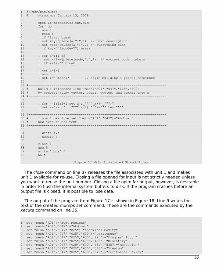
Figure 17 MeSH Structured Global Array

The close command on line 37 releases the file associated with unit 1 and makes unit 1 available for re-use. Closing a file opened for input is not strictly needed unless you want to reuse the unit number. Closing a file open for output, however, is desirable in order to flush the internal system buffers to disk. If the program crashes before an output file is closed, it is possible to lose data.

The output of the program from Figure 17 is shown in Figure 18. Line 9 writes the text of the created mumps set command. These are the commands executed by the xecute command on line 35.

1 set ^mesh("A01")="Body Regions"2 set ^mesh("A01","047")="Abdomen"3 set ^mesh("A01","047","025")="Abdominal Cavity"4 set ^mesh("A01","047","025","600")="Peritoneum"5 set ^mesh("A01","047","025","600","225")="Douglas' Pouch"6 set ^mesh("A01","047","025","600","451")="Mesentery"7 set ^mesh("A01","047","025","600","451","535")="Mesocolon"8 set ^mesh("A01","047","025","600","573")="Omentum"9 set ^mesh("A01","047","025","600","678")="Peritoneal Cavity"

27

10 set ^mesh("A01","047","025","750")="Retroperitoneal Space"11 set ^mesh("A01","047","050")="Abdominal Wall"12 set ^mesh("A01","047","365")="Groin"13 set ^mesh("A01","047","412")="Inguinal Canal"14 set ^mesh("A01","047","849")="Umbilicus"15 set ^mesh("A01","176")="Back"16 set ^mesh("A01","176","519")="Lumbosacral Region"17 set ^mesh("A01","176","780")="Sacrococcygeal Region"18 set ^mesh("A01","236")="Breast"19 set ^mesh("A01","236","500")="Nipples"20 set ^mesh("A01","378")="Extremities"21 set ^mesh("A01","378","100")="Amputation Stumps"22 set ^mesh("A01","378","610")="Lower Extremity"23 set ^mesh("A01","378","610","100")="Buttocks"24 set ^mesh("A01","378","610","250")="Foot"25 set ^mesh("A01","378","610","250","149")="Ankle"26 set ^mesh("A01","378","610","250","300")="Forefoot, Human"27 set ^mesh("A01","378","610","250","300","480")="Metatarsus"28 .29 .30 .

Figure 18 Creating the Mesh tree

4.3 Displaying the MeSH Global Array Part I

Now that the MeSH global array has been created, the question is, how to print it, properly indented to show the tree structure of the data.

Figure 21 gives one way to print the global array and the results are shown in Figure 20. In this example we have successively nested loops to print data at lower levels. When data is printed, it is indented by 0, 5, 10, and 15 spaces to reflect the level of the data.

1 #!/usr/bin/mumps2 # mtreeprint.mps January 13, 20083 for lev1=$order(^mesh(lev1)) do4 . write lev1," ",^mesh(lev1),!5 . for lev2=$order(^mesh(lev1,lev2)) do6 .. write ?5,lev2," ",^mesh(lev1,lev2),!7 .. for lev3=$order(^mesh(lev1,lev2,lev3)) do8 ... write ?10,lev3," ",^mesh(lev1,lev2,lev3),!9 ... for lev4=$order(^mesh(lev1,lev2,lev3,lev4)) do10 .... write ?15,lev4," ",^mesh(lev1,lev2,lev3,lev4),!

Figure 19 Program to print MeSH tree

On Line 3 the process begins by finding successive values of the first index of ^mesh. Each iteration of this outermost loop will yield, in alphabetic order, a new top level value until there are none remaining. These are placed in the local variable lev1.

For each value in lev1, the program prints the index value and the text value stored at the node without indentation. The first line of the output in Figure 20 (A01 Body Regions) is an example of this.

The program then advances to line 5 which will yield successive values of all second level codes subordinate to the current top level code (lev1). Each of these is placed in lev2. The second level codes are printed on line 6 indented by 5 spaces.

28

The process continues for levels 3 and 4. If there are no codes at a given level, the loop at that level terminates and flow is returned to the outer loop. The inner loops, if any, are not executed.

A01 Body Regions 047 Abdomen 025 Abdominal Cavity 600 Peritoneum 750 Retroperitoneal Space 050 Abdominal Wall 365 Groin 412 Inguinal Canal 849 Umbilicus 176 Back 519 Lumbosacral Region 780 Sacrococcygeal Region 236 Breast 500 Nipples 378 Extremities 100 Amputation Stumps 610 Lower Extremity 100 Buttocks 250 Foot 400 Hip 450 Knee 500 Leg 750 Thigh 800 Upper Extremity 075 Arm 090 Axilla 420 Elbow 585 Forearm 667 Hand 750 Shoulder 456 Head 313 Ear 505 Face 173 Cheek 259 Chin 420 Eye 580 Forehead 631 Mouth 733 Nose 750 Parotid Region 810 Scalp 830 Skull Base 150 Cranial Fossa, Anterior 165 Cranial Fossa, Middle 200 Cranial Fossa, Posterior 598 Neck 673 Pelvis 600 Pelvic Floor 719 Perineum 911 Thorax 800 Thoracic Cavity 500 Mediastinum 650 Pleural Cavity 850 Thoracic Wall 960 VisceraA02 Musculoskeletal System 165 Cartilage 165 Cartilage, Articular 207 Ear Cartilages 410 Intervertebral Disk 507 Laryngeal Cartilages

29

083 Arytenoid Cartilage 211 Cricoid Cartilage 411 Epiglottis 870 Thyroid Cartilage 590 Menisci, Tibial 639 Nasal Septum 340 Fascia 424 Fascia Lata 513 Ligaments 170 Broad Ligament 514 Ligaments, Articular 100 Anterior Cruciate Ligament 162 Collateral Ligaments 287 Ligamentum Flavum 350 Longitudinal Ligaments 475 Patellar Ligament 600 Posterior Cruciate Ligament

.

.

.

Figure 20 Printed the Mesh tree

4.4 Printing the MeSH Global Array Part II

Using the example from Figure 24 we can now write a more general function to print the ^mesh hierarchy as shown in Figure 21.

1 #!/usr/bin/mumps2 # mtreeprintnew.mps January 28, 20103 set x="^mesh"4 for do5 . set x=$query(x)6 . if x="" break7 . set i=$qlength(x)8 . write ?i*2," ",$qsubscript(x,i)," ",@x,?50,x,!

Figure 21 Alternate MeSH tree printing program

In the example in Figure 21, we first set a local variable x to ^mesh, the unindexed name of the MeSH global array. In the loop on lines 4 through 8, the variable x is passed as an argument to the builtin function $query() which returns the next ascendant global array key in the database. These can be seen in the right hand column output in Figure 22. These are re-assigned to the variable x.

In line 7 the number of subscripts in the global array reference in variable x is assigned to the local variable i. In line 8 this number is used to indent the output by twice the number os spaces as there are subscripts (?i*2).

The $qsubscript() function returns the value of the ith subscript (e.g., A01). The expression @x evaluates the string in variable x which, since it is a global array reference, evaluates to the value stored at the global array node which is the MeSH text description. The actual MeSH global array reference is then printed in a column to the right.

A01 Body Regions ^mesh("A01") 047 Abdomen ^mesh("A01","047") 025 Abdominal Cavity ^mesh("A01","047","025") 600 Peritoneum ^mesh("A01","047","025","600")

30

225 Douglas' Pouch ^mesh("A01","047","025","600","225") 451 Mesentery ^mesh("A01","047","025","600","451") 535 Mesocolon ^mesh("A01","047","025","600","451","535") 573 Omentum ^mesh("A01","047","025","600","573") 678 Peritoneal Cavity ^mesh("A01","047","025","600","678") 750 Retroperitoneal Space ^mesh("A01","047","025","750") 050 Abdominal Wall ^mesh("A01","047","050") 365 Groin ^mesh("A01","047","365") 412 Inguinal Canal ^mesh("A01","047","412") 849 Umbilicus ^mesh("A01","047","849") 176 Back ^mesh("A01","176") 519 Lumbosacral Region ^mesh("A01","176","519") 780 Sacrococcygeal Region ^mesh("A01","176","780") 236 Breast ^mesh("A01","236") 500 Nipples ^mesh("A01","236","500") 378 Extremities ^mesh("A01","378") 100 Amputation Stumps ^mesh("A01","378","100") 610 Lower Extremity ^mesh("A01","378","610") 100 Buttocks ^mesh("A01","378","610","100") 250 Foot ^mesh("A01","378","610","250") 149 Ankle ^mesh("A01","378","610","250","149") 300 Forefoot, Human ^mesh("A01","378","610","250","300") 480 Metatarsus ^mesh("A01","378","610","250","300","480") 792 Toes ^mesh("A01","378","610","250","300","792") 380 Hallux ^mesh("A01","378","610","250","300","792","380") 510 Heel ^mesh("A01","378","610","250","510") 400 Hip ^mesh("A01","378","610","400") 450 Knee ^mesh("A01","378","610","450") 500 Leg ^mesh("A01","378","610","500") 750 Thigh ^mesh("A01","378","610","750") 800 Upper Extremit ^mesh("A01","378","800") 075 Arm ^mesh("A01","378","800","075") 090 Axilla ^mesh("A01","378","800","090") 420 Elbow ^mesh("A01","378","800","420") 585 Forearm ^mesh("A01","378","800","585") 667 Hand ^mesh("A01","378","800","667") 430 Fingers ^mesh("A01","378","800","667","430") 705 Thumb ^mesh("A01","378","800","667","430","705") 715 Wrist ^mesh("A01","378","800","667","715") 750 Shoulder ^mesh("A01","378","800","750") 456 Head ^mesh("A01","456") 313 Ear ^mesh("A01","456","313") 505 Face ^mesh("A01","456","505") 173 Cheek ^mesh("A01","456","505","173") 259 Chin ^mesh("A01","456","505","259") 420 Eye ^mesh("A01","456","505","420") 338 Eyebrows ^mesh("A01","456","505","420","338") 504 Eyelids ^mesh("A01","456","505","420","504") 421 Eyelashes ^mesh("A01","456","505","420","504","421") 580 Forehead ^mesh("A01","456","505","580") 631 Mouth ^mesh("A01","456","505","631")515 Lip ^mesh("A01","456","505","631","515")

Figure 22 Alternative MeSH printing output

4.5 Displaying Global Arrays in Key Order

The problem with the program in Figure 19 is that it only prints down to four levels and is very repetitive. Can it be re-written more generally?

Yes, using some of the newer Mumps functions, the MeSH hierarchy can be printed to an arbitrary level of depth without the redundant code from the previous example. But first, we need a way to cycle through each global array index set without all the for loop depths.

31

First we must understand that program in Figure 17 stored the ^mesh keys in the global array b-tree database sequentially in the manner shown in Figure 23.

1 ^mesh("A01") 2 ^mesh("A01","047") 3 ^mesh("A01","047","025") 4 ^mesh("A01","047","025","600") 5 ^mesh("A01","047","025","600","225") 6 ^mesh("A01","047","025","600","451") 7 ^mesh("A01","047","025","600","451","535") 8 ^mesh("A01","047","025","600","573") 9 ^mesh("A01","047","025","600","678") 10 ^mesh("A01","047","025","750") 11 ^mesh("A01","047","050") 12 ^mesh("A01","047","365") 13 ^mesh("A01","047","412") 14 ^mesh("A01","047","849") 15 ^mesh("A01","176")

Figure 23 MeSH global array codes

The Mumps function $query() can be used access the b-tree keys in the order in which they are actually stored in sequential key order as shown in Figure 23.

The example program shown in Figure 24 passes to $query() a string containing a global array reference. The function returns the next ascending global array reference in the file system. Eventually, it will run out of ^mesh references and receive an empty string. Consequently, it tests to determine if it received the empty string.

Note: the line:

. write x,?50,@x,!

displays the global array reference in variable x and then prints the contents of the node at x by evaluating the global array reference (@x). Evaluation of a variable yields the value of the variable.

1 #!/usr/bin/mumps2 # meshheadings.mps January 28, 20103 set x="^mesh" // build the first index4 for do5 . set x=$query(x) // get next array reference6 . if x="" break7 . write x,?50,@x,!

Figure 24 Program to print MeSH global

The output from Figure 24 appears in Figure 25.

^mesh("A01") Body Regions^mesh("A01","047") Abdomen^mesh("A01","047","025") Abdominal Cavity^mesh("A01","047","025","600") Peritoneum^mesh("A01","047","025","600","225") Douglas' Pouch^mesh("A01","047","025","600","451") Mesentery^mesh("A01","047","025","600","451","535") Mesocolon

32

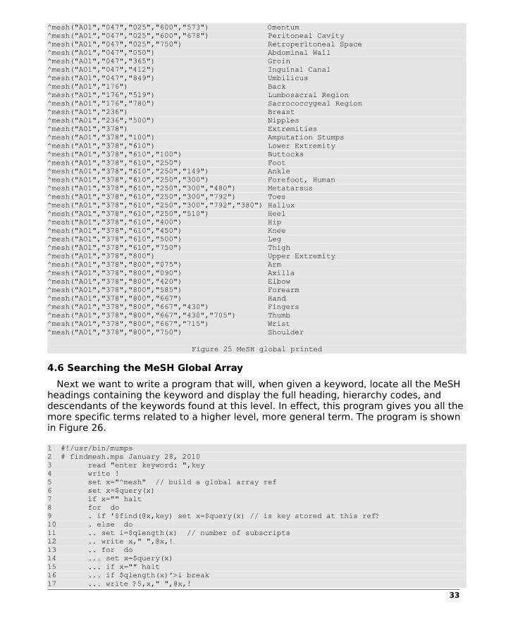
^mesh("A01","047","025","600","573") Omentum^mesh("A01","047","025","600","678") Peritoneal Cavity^mesh("A01","047","025","750") Retroperitoneal Space^mesh("A01","047","050") Abdominal Wall^mesh("A01","047","365") Groin^mesh("A01","047","412") Inguinal Canal^mesh("A01","047","849") Umbilicus^mesh("A01","176") Back^mesh("A01","176","519") Lumbosacral Region^mesh("A01","176","780") Sacrococcygeal Region^mesh("A01","236") Breast^mesh("A01","236","500") Nipples^mesh("A01","378") Extremities^mesh("A01","378","100") Amputation Stumps^mesh("A01","378","610") Lower Extremity^mesh("A01","378","610","100") Buttocks^mesh("A01","378","610","250") Foot^mesh("A01","378","610","250","149") Ankle^mesh("A01","378","610","250","300") Forefoot, Human^mesh("A01","378","610","250","300","480") Metatarsus^mesh("A01","378","610","250","300","792") Toes^mesh("A01","378","610","250","300","792","380") Hallux^mesh("A01","378","610","250","510") Heel^mesh("A01","378","610","400") Hip^mesh("A01","378","610","450") Knee^mesh("A01","378","610","500") Leg^mesh("A01","378","610","750") Thigh^mesh("A01","378","800") Upper Extremity^mesh("A01","378","800","075") Arm^mesh("A01","378","800","090") Axilla^mesh("A01","378","800","420") Elbow^mesh("A01","378","800","585") Forearm^mesh("A01","378","800","667") Hand^mesh("A01","378","800","667","430") Fingers^mesh("A01","378","800","667","430","705") Thumb^mesh("A01","378","800","667","715") Wrist^mesh("A01","378","800","750") Shoulder

Figure 25 MeSH global printed

4.6 Searching the MeSH Global Array

Next we want to write a program that will, when given a keyword, locate all the MeSH headings containing the keyword and display the full heading, hierarchy codes, and descendants of the keywords found at this level. In effect, this program gives you all the more specific terms related to a higher level, more general term. The program is shown in Figure 26.

1 #!/usr/bin/mumps2 # findmesh.mps January 28, 20103 read "enter keyword: ",key4 write !5 set x="^mesh" // build a global array ref6 set x=$query(x)7 if x="" halt8 for do9 . if '$find(@x,key) set x=$query(x) // is key stored at this ref?10 . else do11 .. set i=$qlength(x) // number of subscripts12 .. write x," ",@x,!13 .. for do14 ... set x=$query(x) 15 ... if x="" halt16 ... if $qlength(x)'>i break17 ... write ?5,x," ",@x,!

33

18 . if x="" halt

Figure 26 Program to search MeSH global array

The program in Figure 26 first reads in a keyword into a local variable key then builds in local variable x a global array reference containing an initial key ^mesh. Next it locates the first index of this global array with $query() as was done in the examples above.

In the loop at lines through 18 the program examines each of the global array nodes in ^mesh in global array key order. In line 9, the $find() function determines if the value stored at the global array node referenced by x (@x) contains, as a substring, the value in key.

If $find() does not detect the value in key in the global array node, the next global array reference is found with $query() and the process repeats until there are no more global array nodes to be checked.

If the key is found, however, it prints the reference and scans for additional references whose number of subscripts is greater than that of the found reference (sub trees of the found reference). That is, it prints any nodes that are subordinate to the found node since these are necessarily more specific forms of the term being sought. The function $qlength() returns the number of subscripts in a reference. When the number of subscripts becomes less-than-or-equal (shown as not-greater-than: '>) to the number of subscripts in the found reference, printing ends and the key scan of the nodes resumes. Thus, only sub-trees of the found nodes will be printed.

The result of a search is shown in Figure 27 where Skeleton was given as input.

enter keyword: Skeleton^mesh("A02","835") Skeleton^mesh("A02","835","232") Bone and Bones^mesh("A02","835","232","087") Bones of Upper Extremity^mesh("A02","835","232","087","144") Carpal Bones^mesh("A02","835","232","087","144","650") Scaphoid Bone^mesh("A02","835","232","087","144","663") Semilunar Bone^mesh("A02","835","232","087","227") Clavicle^mesh("A02","835","232","087","412") Humerus^mesh("A02","835","232","087","535") Metacarpus^mesh("A02","835","232","087","702") Radius^mesh("A02","835","232","087","783") Scapula^mesh("A02","835","232","087","783","261") Acromion^mesh("A02","835","232","087","911") Ulna^mesh("A02","835","232","169") Diaphyses^mesh("A02","835","232","251") Epiphyses^mesh("A02","835","232","251","352") Growth Plate^mesh("A02","835","232","300") Foot Bones^mesh("A02","835","232","300","492") Metatarsal Bones^mesh("A02","835","232","300","710") Tarsal Bones^mesh("A02","835","232","300","710","300") Calcaneus^mesh("A02","835","232","300","710","780") Talus^mesh("A02","835","232","409") Hyoid Bone^mesh("A02","835","232","500") Leg Bones^mesh("A02","835","232","500","247") Femur^mesh("A02","835","232","500","247","343") Femur Head^mesh("A02","835","232","500","247","510") Femur Neck^mesh("A02","835","232","500","321") Fibula^mesh("A02","835","232","500","624") Patella^mesh("A02","835","232","500","883") Tibia

34

^mesh("A02","835","232","611") Pelvic Bones^mesh("A02","835","232","611","108") Acetabulum^mesh("A02","835","232","611","434") Ilium^mesh("A02","835","232","611","548") Ischium^mesh("A02","835","232","611","781") Pubic Bone^mesh("A02","835","232","730") Sesamoid Bones^mesh("A02","835","232","781") Skull^mesh("A02","835","232","781","200") Cranial Sutures^mesh("A02","835","232","781","292") Ethmoid Bone^mesh("A02","835","232","781","324") Facial Bones^mesh("A02","835","232","781","324","502") Jaw^mesh("A02","835","232","781","324","502","125") Alveolar Process^mesh("A02","835","232","781","324","502","125","800") Tooth Socket^mesh("A02","835","232","781","324","502","320") Dental Arch^mesh("A02","835","232","781","324","502","632") Mandible^mesh("A02","835","232","781","324","502","632","130") Chin^mesh("A02","835","232","781","324","502","632","600") Mandibular Condyle^mesh("A02","835","232","781","324","502","645") Maxilla^mesh("A02","835","232","781","324","502","660") Palate, Hard^mesh("A02","835","232","781","324","665") Nasal Bone^mesh("A02","835","232","781","324","690") Orbit^mesh("A02","835","232","781","324","948") Turbinates^mesh("A02","835","232","781","324","995") Zygoma^mesh("A02","835","232","781","375") Frontal Bone^mesh("A02","835","232","781","572") Occipital Bone^mesh("A02","835","232","781","572","434") Foramen Magnum^mesh("A02","835","232","781","651") Parietal Bone^mesh("A02","835","232","781","750") Skull Base^mesh("A02","835","232","781","750","150") Cranial Fossa, Anterior^mesh("A02","835","232","781","750","165") Cranial Fossa, Middle^mesh("A02","835","232","781","750","400") Cranial Fossa, Posterior^mesh("A02","835","232","781","802") Sphenoid Bone^mesh("A02","835","232","781","802","662") Sella Turcica^mesh("A02","835","232","781","885") Temporal Bone^mesh("A02","835","232","781","885","444") Mastoid^mesh("A02","835","232","781","885","681") Petrous Bone^mesh("A02","835","232","834") Spine^mesh("A02","835","232","834","151") Cervical Vertebrae^mesh("A02","835","232","834","151","213") Atlas^mesh("A02","835","232","834","151","383") Axis^mesh("A02","835","232","834","151","383","668") Odontoid Process^mesh("A02","835","232","834","229") Coccyx^mesh("A02","835","232","834","432") Intervertebral Disk^mesh("A02","835","232","834","519") Lumbar Vertebrae^mesh("A02","835","232","834","717") Sacrum^mesh("A02","835","232","834","803") Spinal Canal^mesh("A02","835","232","834","803","350") Epidural Space^mesh("A02","835","232","834","892") Thoracic Vertebrae^mesh("A02","835","232","904") Thorax^mesh("A02","835","232","904","567") Ribs^mesh("A02","835","232","904","766") Sternum^mesh("A02","835","232","904","766","442") Manubrium^mesh("A02","835","232","904","766","825") Xiphoid Bone^mesh("A02","835","583") Joints^mesh("A02","835","583","032") Acromioclavicular Joint^mesh("A02","835","583","097") Atlanto-Axial Joint^mesh("A02","835","583","101") Atlanto-Occipital Joint^mesh("A02","835","583","156") Bursa, Synovial^mesh("A02","835","583","192") Cartilage, Articular^mesh("A02","835","583","290") Elbow Joint^mesh("A02","835","583","345") Finger Joint^mesh("A02","835","583","345","512") Metacarpophalangeal Joint^mesh("A02","835","583","378") Foot Joints^mesh("A02","835","583","378","062") Ankle Joint^mesh("A02","835","583","378","531") Metatarsophalangeal Joint^mesh("A02","835","583","378","831") Tarsal Joints

35

^mesh("A02","835","583","378","831","780") Subtalar Joint^mesh("A02","835","583","378","900") Toe Joint^mesh("A02","835","583","411") Hip Joint^mesh("A02","835","583","443") Joint Capsule^mesh("A02","835","583","443","800") Synovial Membrane^mesh("A02","835","583","443","800","800") Synovial Fluid^mesh("A02","835","583","475") Knee Joint^mesh("A02","835","583","475","590") Menisci, Tibial^mesh("A02","835","583","512") Ligaments, Articular^mesh("A02","835","583","512","100") Anterior Cruciate Ligament^mesh("A02","835","583","512","162") Collateral Ligaments^mesh("A02","835","583","512","162","500") Lateral Ligament, Ankle^mesh("A02","835","583","512","162","600") Medial Collateral Ligament, Knee^mesh("A02","835","583","512","287") Ligamentum Flavum^mesh("A02","835","583","512","350") Longitudinal Ligaments^mesh("A02","835","583","512","475") Patellar Ligament^mesh("A02","835","583","512","600") Posterior Cruciate Ligament^mesh("A02","835","583","656") Pubic Symphysis^mesh("A02","835","583","707") Sacroiliac Joint^mesh("A02","835","583","748") Shoulder Joint^mesh("A02","835","583","781") Sternoclavicular Joint^mesh("A02","835","583","790") Sternocostal Joints^mesh("A02","835","583","861") Temporomandibular Joint^mesh("A02","835","583","861","900") Temporomandibular Joint Disk^mesh("A02","835","583","959") Wrist Joint^mesh("A02","835","583","979") Zygapophyseal Joint^mesh("A11","284","295","154","200") Cell Wall Skeleton^mesh("D12","776","097","162") Cell Wall Skeleton^mesh("D12","776","395","560","186") Cell Wall Skeleton^mesh("E01","370","350","700","050") Age Determination by Skeleton

Figure 27 MeSH keyword search results

4.7 Web Browser Search of the MeSH Global Array

Now let us make the program from Figure 26 run as a web server based information storage and retrieval application. The code for this is shown in Figures 28 and 29.

The first of these, Figure 28, gives the initial static HTML code to display a form on the users browser. The resulting display is shown in Figure 30. The second, in Figure 29, gives the server side Mumps program to process the query and return the results, formatted in HTML, to the user's browser. The result of this program is shown in Figure 31.

1 <html>2 <!-- isr.html -->3 <head>4 <title> Example server side Mumps Program </title>5 </head>6 <body bgcolor=silver>7 Enter a MeSH term: &nbsp;8 <form method="get" action="cgi-bin/isr.mps">9 <input type="text" size=30 name="key" value="Head">10 &nbsp;11 <input type="submit">12 </form>13 </body>14 </html>

Figure 28 HTML <FORM> example

In order to run programs through your web server, you must place them in certain locations. These may vary depending on the version of Linux you are using.

36

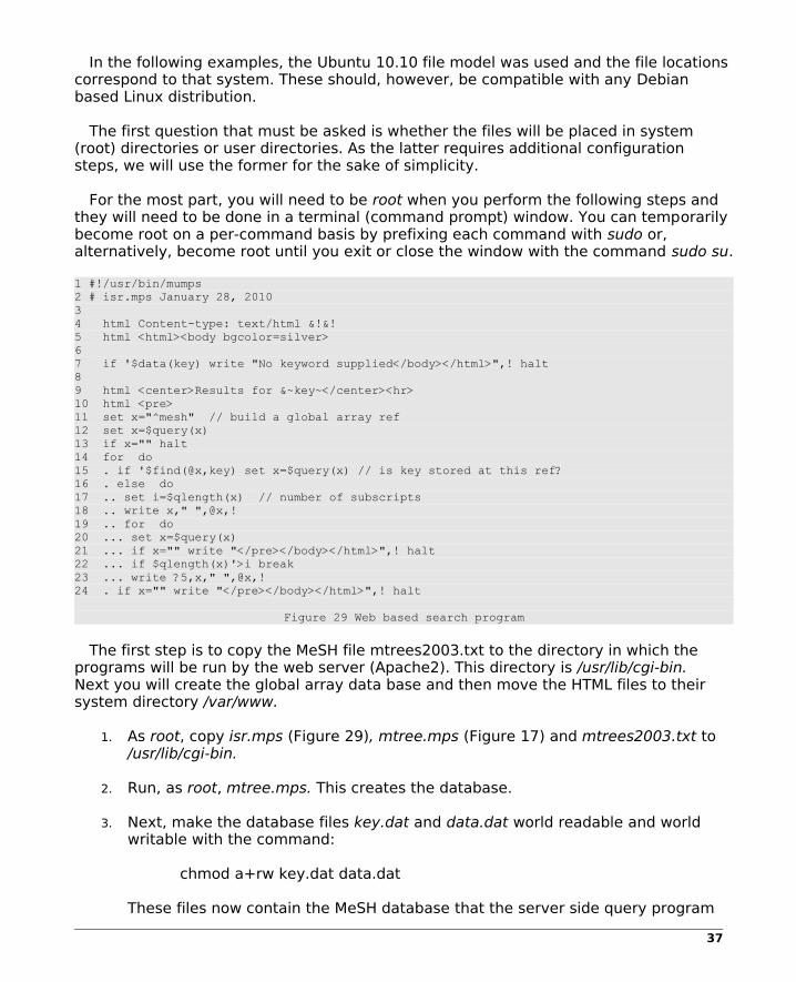
In the following examples, the Ubuntu 10.10 file model was used and the file locations correspond to that system. These should, however, be compatible with any Debian based Linux distribution.

The first question that must be asked is whether the files will be placed in system (root) directories or user directories. As the latter requires additional configuration steps, we will use the former for the sake of simplicity.

For the most part, you will need to be root when you perform the following steps and they will need to be done in a terminal (command prompt) window. You can temporarily become root on a per-command basis by prefixing each command with sudo or, alternatively, become root until you exit or close the window with the command sudo su.

1 #!/usr/bin/mumps2 # isr.mps January 28, 20103 4 html Content-type: text/html &!&!5 html <html><body bgcolor=silver>6 7 if '$data(key) write "No keyword supplied</body></html>",! halt8 9 html <center>Results for &~key~</center><hr>10 html <pre>11 set x="^mesh" // build a global array ref12 set x=$query(x)13 if x="" halt14 for do15 . if '$find(@x,key) set x=$query(x) // is key stored at this ref?16 . else do17 .. set i=$qlength(x) // number of subscripts18 .. write x," ",@x,!19 .. for do20 ... set x=$query(x)21 ... if x="" write "</pre></body></html>",! halt22 ... if $qlength(x)'>i break23 ... write ?5,x," ",@x,!24 . if x="" write "</pre></body></html>",! halt

Figure 29 Web based search program

The first step is to copy the MeSH file mtrees2003.txt to the directory in which the programs will be run by the web server (Apache2). This directory is /usr/lib/cgi-bin. Next you will create the global array data base and then move the HTML files to their system directory /var/www.

1. As root, copy isr.mps (Figure 29), mtree.mps (Figure 17) and mtrees2003.txt to /usr/lib/cgi-bin.

2. Run, as root, mtree.mps. This creates the database.

3. Next, make the database files key.dat and data.dat world readable and world writable with the command:

chmod a+rw key.dat data.dat

These files now contain the MeSH database that the server side query program

37

isr.mps will access.

4. Copy isr.html to /var/www and make sure it's world readable:

chmod a+r isr.html

You should now be able to access the initial form page with the URL:

127.0.0.1/isr.html The result should look like the example in Figure 30.

How does this work?

1. First, the HTML file isr.html creates the display on the user's browser containing an HTML form that is used to collect information as seen in Figure 30. The HTML <FORM> tag can be used to collect one or more single lines of text, a boxes of text, radio buttons, check boxes and selection lists (drop down boxes). Each item of data collected, upon clicking the SUBMIT button, is sent to the web server. In this example, however, only a line of text is to be collected.

2. A form consists of one or more <INPUT> tags. These can can be sued to collect text, radio button and check box status and select box selection. They can also be used to embed hidden data which will not appear on the user's screen but will be sent to the web server. The type of input to be collected is specified in the type= field.

3. Each <INPUT> tag in a form collects data to be submitted to the web server. The name= field in the <INPUT> tag is how you specify the name the data item will be known to the web server by and the value= field, if available, allows you to provide an initial or default value for the item as it displays on the user's browser. In the cases of check boxes, radio buttons and select boxes, there is no value= field but, instead, a way to select a default check or selection.

4. When the user at the browser enters text or selects a box or button and then clicks SUBMIT, the information is collected by the browser and sent to the web server. There are two ways this information can be sent. These are specified in the method= field of the <FORM> tag. The POST method sends the data separate from the URL while the GET method attaches the data to the URL. The GET method limits the amount of data that can be sent and allows the user to see it in the URL bar. POST does not display the data and has no size restriction. There are advantages to both methods. GET permits the page and it's parameters to be bookmarked whereas POST only allows the main part of the URL to be bookmarked. GET is better for debugging as it allows the developer to see the data being sent. In Mumps, only GET is presently supported.

5. In the GET method, the strings collected as a result of the <INPUT> tags are encoded by the browser: alphabetics and numerics remain unchanged; blanks become plus signs while most other characters appear in the form %XX where XX is a hexadecimal number indicating the character's collating sequence value.

38

6. In GET method, each <INPUT> tag generates an entry appended to the URL. The If more than one name= value figures is appended to the URL, they, are separated from one another by and ampersand (&).

The interpreter automatically reads QUERY_STRING (which contains the parameters following the question mark) and decodes them. For each "name" found, it creates a variable of the same name in the Mumps run-time symbol table initialized to the "value" field. Names should be unique although non-unique names can be handled (see the manual).

When your CGI program runs, its output is captured by the web server and sent back to the originating browser. The first thing you send to the web server MUST be the line:

html Content-type: text/html &!&!

exactly as typed. This tells the web server what's coming next. After this line, everything sent would be in HTML format. The Mumps command "html" is an output command that causes the remainder of the line to be written to the web server. Write commands can also be used but the text requires a lot of annoying quote marks. You may embed in the HTML line figures of the form:

&! and &~expression~

Figure 30 Browser display of <FORM> tag

The first of these, &!, causes a new line. The second causes evaluation of the expression and the result to be written to the web server (the &~ and ~ are not sent).

Now open a browser and enter: 39

127.0.0.1/cgi-bin/isr.html

This will bring up the first screen shown in Figure 30. Click Submit Query and the second screen shown in Figure 31 will appear.

Figure 31 Browser display of results

The HTML code in Figure 32 illustrates most of the major <FORM> data collection techniques and produces the screencap shown in Figure 33.

1 <form method="get" action="quiz2.cgi">2 3 <center>4 Name: 5 <input type="text" name="name" size=40 value=""><br>6 </center>7 8 Class:9 <input type="Radio" name="class" value="freshman" > Freshman10 <input type="Radio" name="class" value="sophomore" > Sophomore11 <input type="Radio" name="class" value="junior" > Junior12 <input type="Radio" name="class" value="senior" checked> Senior13 <input type="Radio" name="class" value="grad" > Grad Student14 15 <br>16 Major:17 <select name="major" size=7>18 <option value="computer science" >computer science19 <option value="mathematics" >Mathematics

40

20 <option value="biology" selected>Biology21 <option value="chemistry" >Chemistry22 <option value="earth science" >Earth Science23 <option value="industrial technology" >Industrial Technology24 25 <option value="physics" >Physics26 </select>27 28 <table border>29 <tr>30 <td valign=top>31 Hobbies:32 </td>33 <td>34 <input type="Checkbox" name="hobby1" value="stamp collecting" > 35 Stamp Collecting<br>36 <input type="Checkbox" name="hobby2" value="art" > Art<br>37 <input type="Checkbox" checked name="hobby3" value="bird watching" 38 > Bird Watching<br>39 40 <input type="Checkbox" name="hobby4" value="hang gliding" > Hang 41 Gliding<br>42 <input type="Checkbox" name="hobby5" value="reading" > 43 Reading<br>44 </td></tr>45 </table>46 47 <center>48 <input type="submit" value="go for it">49 </center>50 </form>

Figure 32 Example <FORM> input types

Figure 33 Browser display of Figure 32

41

The web site:

http://werbach.com/barebones/

for a good synopsis of many HTML commands.

4.8 Indexing OHSUMED by MeSH Headings

Next, we want to write a program to read MEDLINE formatted abstracts (from the modified TREC-9 data base described above) and write out a list of MeSH headings, the number of times each occurs, and the title of each abstract in which it occurs along with the byte offset of the abstract in the master file.

This is an example of an inverted index, that is, a mapping from a collection of index terms, in this case the MeSH headings, to the underlying documents containing these headings. An inverted index is faster than sequentially searching each document for index terms.

First note that the lines with MeSH headings in the OHSUMED data base all have the code MH in positions 1 and 2. Note also that there is a blank line that signals the end of each abstract and the beginning of the next one (or the end of file).

Creation of the inverted index proceeds as follows: first, we locate all the MeSH terms in the OHSUMED file and then, for each instance of a MeSH term, we record the term and the offset into the OHSUMED file of the article where the term occurred in a global array (^MH). Additionally, we count the number of times we see each term. The program to do all this is in Figure 34.

Ultimately, after the entire OHSUMED file has been processed, we write out each MeSH heading, the number of times it occurs and a list of the titles and their offsets. An example of the output can be seen in Figure 35.

1 #!/usr/bin/mumps 2 3 # meshinvert.mps Feb 1, 20114 5 open 1:"osu.medline,old" 6 use 1 7 8 kill ^MH 9 10 set x=0 // a counter to limit the size 11 12 set i=$ztell // return the integer offset in the file 13 14 for do 15 . use 1 16 . read a 17 . if '$test break 18 19 # if a blank line, record the offset - this is the start of an abstract 20 21 . if a="" set i=$ztell set x=x+1 quit // return the offset in the file 22 23 . if $extract(a,1,3)="MH " do 24 .. use 5 25 .. set a=$piece($extract(a,7,255),"/",1)

42

26 27 # create or increment entry for word 28 29 .. if $data(^MH(a)) set ^MH(a)=^MH(a)+1 30 .. else set ^MH(a)=1 31 32 # store the offset 33 34 .. set ^MH(a,i)="" 35 36 # write for each heading the titles associated with it 37 38 use 5 39 set x="" 40 for do 41 . set x=$order(^MH(x)) 42 . if x="" break 43 . write x," occurs in ",^MH(x)," documents",! 44 . for off=$order(^MH(x,off)) do 45 .. use 1 46 .. do $zseek(off) 47 .. for do 48 ... read a 49 ... if $extract(a,1,3)'="TI " quit 50 ... use 5 51 ... write ?5,off,?15,$extract(a,7,80),! 52 ... break

Figure 34 Locate instances of MeSH keywords

The program opens the input file (line 5), captures the initial file byte offset (line 12) and then loops reading lines from the input file designated as unit 1. The loop ends when there is no more input.

If an empty line is detected (line 21), the offset is recorded in the local variable i, the abstract count x is incremented. The value returned by $ftell() is the byte offset of the line about to be read, not the one most recently read. Thus, the value in variable i is the address of the first line of the next abstract.

Line 23 checks to see if each line contains the code MH. If it does, it extracts the portion of the line from position 7 up to, but not including, any / character (we ignore any text following the / character). If no / character is present, we extract to end of line. The line length limit of 255 is overly generous as no line is that long. The actual length of the MeSH heading in local variable a is determined by the actual line length, not 255. Next the MeSH heading, a pound sign and the offset are written to standard output. For each MeSH heading detected, the count in ^MH for the term is incremented (lines 29 and 30) and the offset of the document containing it is recorded (line 34).

When the input is exhausted, the program prints for each heading the number of documents it appeared in along with a list of the documents. A sample of the output is given in Figure 35. This form of display is called a concordance - a list of words and an indication of their location and context.

Abdominal Injuries occurs in 13 documents 1650173 Percutaneous transcatheter steel-coil embolization of a large proximal pos 1678059 Features of 164 bladder ruptures. 2523966 Injuries to the abdominal vascular system: how much does aggressive resusc 3436121 Triple-contrast computed tomography in the evaluation of penetrating poste 4624903 Correlations of injury, toxicology, and cause of death to Galaxy Flight 20

43

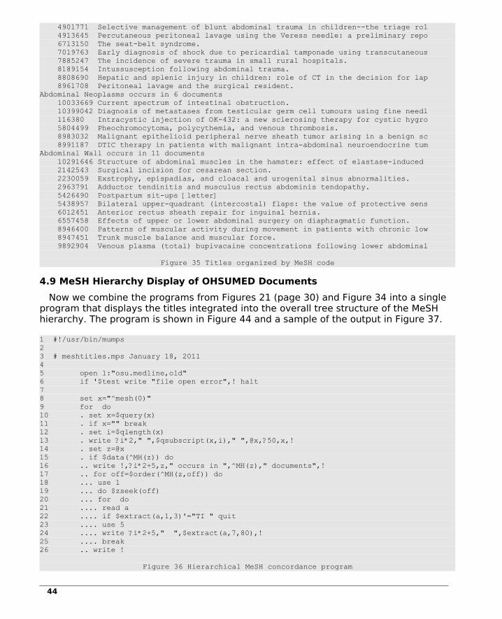
4901771 Selective management of blunt abdominal trauma in children--the triage rol 4913645 Percutaneous peritoneal lavage using the Veress needle: a preliminary repo 6713150 The seat-belt syndrome. 7019763 Early diagnosis of shock due to pericardial tamponade using transcutaneous 7885247 The incidence of severe trauma in small rural hospitals. 8189154 Intussusception following abdominal trauma. 8808690 Hepatic and splenic injury in children: role of CT in the decision for lap 8961708 Peritoneal lavage and the surgical resident.Abdominal Neoplasms occurs in 6 documents 10033669 Current spectrum of intestinal obstruction. 10399042 Diagnosis of metastases from testicular germ cell tumours using fine needl 116380 Intracystic injection of OK-432: a new sclerosing therapy for cystic hygro 5804499 Pheochromocytoma, polycythemia, and venous thrombosis. 8983032 Malignant epithelioid peripheral nerve sheath tumor arising in a benign sc 8991187 DTIC therapy in patients with malignant intra-abdominal neuroendocrine tumAbdominal Wall occurs in 11 documents 10291646 Structure of abdominal muscles in the hamster: effect of elastase-induced 2142543 Surgical incision for cesarean section. 2230059 Exstrophy, epispadias, and cloacal and urogenital sinus abnormalities. 2963791 Adductor tendinitis and musculus rectus abdominis tendopathy. 5426490 Postpartum sit-ups [letter] 5438957 Bilateral upper-quadrant (intercostal) flaps: the value of protective sens 6012451 Anterior rectus sheath repair for inguinal hernia. 6557458 Effects of upper or lower abdominal surgery on diaphragmatic function. 8946400 Patterns of muscular activity during movement in patients with chronic low 8947451 Trunk muscle balance and muscular force. 9892904 Venous plasma (total) bupivacaine concentrations following lower abdominal

Figure 35 Titles organized by MeSH code

4.9 MeSH Hierarchy Display of OHSUMED Documents

Now we combine the programs from Figures 21 (page 30) and Figure 34 into a single program that displays the titles integrated into the overall tree structure of the MeSH hierarchy. The program is shown in Figure 44 and a sample of the output in Figure 37.

1 #!/usr/bin/mumps 2 3 # meshtitles.mps January 18, 2011 4 5 open 1:"osu.medline,old" 6 if '$test write "file open error",! halt 7 8 set x="^mesh(0)" 9 for do 10 . set x=$query(x) 11 . if x="" break 12 . set i=$qlength(x) 13 . write ?i*2," ",$qsubscript(x,i)," ",@x,?50,x,! 14 . set z=@x 15 . if $data(^MH(z)) do 16 .. write !,?i*2+5,z," occurs in ",^MH(z)," documents",! 17 .. for off=$order(^MH(z,off)) do 18 ... use 1 19 ... do $zseek(off) 20 ... for do 21 .... read a 22 .... if $extract(a,1,3)'="TI " quit 23 .... use 5 24 .... write ?i*2+5," ",$extract(a,7,80),! 25 .... break 26 .. write !

Figure 36 Hierarchical MeSH concordance program

44

025 Abdominal Cavity ^mesh("A01","047","025") 600 Peritoneum ^mesh("A01","047","025","600")

Peritoneum occurs in 4 documents Systems of membranes involved in peritoneal dialysis. Suppression of lymphocyte reactivity in vitro by supernatants of explants An evaluation of the Gore-Tex surgical membrane for the prevention of post The morphologic effect of short-term medical therapy of endometriosis.

225 Douglas' Pouch ^mesh("A01","047","025","600","225") 451 Mesentery ^mesh("A01","047","025","600","451")

Mesentery occurs in 3 documents Cellular localization of angiotensinogen gene expression in brown adipose Technique of mesenteric lengthening in ileal reservoir-anal anastomosis. Detection of mesenteric involvement in sarcoidosis using computed tomograp

535 Mesocolon ^mesh("A01","047","025","600","451","535") 573 Omentum ^mesh("A01","047","025","600","573")

Omentum occurs in 5 documents The omentum as an untapped reservoir for microvascular conduits. Early vascular grafting to prevent upper extremity necrosis after electric Evidence for an inhibitor of leucocyte sodium transport in the serum of ne Vascular graft seeding [letter] Suppression of lymphocyte reactivity in vitro by supernatants of explants

678 Peritoneal Cavity ^mesh("A01","047","025","600","678")

Peritoneal Cavity occurs in 4 documents Contribution of lymphatic absorption to loss of ultrafiltration and solute Differential expression of the amyloid SAA 3 gene in liver and peritoneal The pharmacology of intraperitoneally administered bleomycin. Ultrafiltration failure in continuous ambulatory peritoneal dialysis due t

750 Retroperitoneal Space ^mesh("A01","047","025","750")

Retroperitoneal Space occurs in 5 documents Failure of adjuvant chemotherapy in testicular cancer. Uterine leiomyomas with retroperitoneal lymph node involvement. Triple-contrast computed tomography in the evaluation of penetrating poste Position of the superior mesenteric artery on computed tomography and its Lumbar arterial injury: radiologic diagnosis and management.

Figure 37 Hierarchical MeSH concordance

4.10 Database Compression

As is the case with many data base systems, once disk blocks have been allocated, they remain as permanent parts of the file system, even if, due to deletions, they are no longer needed. In some systems, this results in an accumulation of unused blocks. In a B-tree based system such as used in Mumps, block occupancy can vary considerably after many deletions and reorganizations.

In order to remove unused blocks and rebuild the B-tree with blocks that are mostly half filled, the data base should be dumped to a sequential, collated ASCII file, the old data base (key.dat and data.dat) erased and then the data base restored from the ACSII file.

There are two functions in Mumps to accomplish this: $zdump() and $zrestore(). The first of these, $zdump() writes the full data base to disk as an ASCII file. If given a string parameter, it will use the contents of the string as the file name. If no file name

45

is given, the default will be the system time in seconds followed by ".dmp". The second function, $zrestore() restores the data base. If given a file name parameter, it will load from the file specified. If no parameter is given, it will look for a file named "dump".

For example, in a large run of 25,000 abstracts which included creation and pruning of the ^doc(), ^index(), ^idf(), ^mca(), ^df() and ^dict() vectors as well as creation of ^tt() and ^dd() matrices (discussed below), the global array data base was:

-rw-rw-rw- 1 root root 19M Mar 5 04:40 /d1/isr/code/data.dat-rw-rw-rw- 1 root root 262M Mar 5 04:40 /d1/isr/code/key.dat

After a dump/restore cycle it was:

-rw-rw-rw- 1 root root 8.5M Mar 5 09:52 data.dat-rw-rw-rw- 1 root root 107M Mar 5 09:52 key.dat

The intermediate dump file was 38M bytes in length. In this case, the dump/restore resulted in more than 2 to 1 in savings and, consequently, faster access due to fewer blocks searched. Figure 38 details the steps.

run the program:

#!/usr/bin/mumps # # dump the data base # do $zdump

followed by the system command:

mv 11100370.dmp dump

which renames the dump data set, followed by the system commands:

rm key.dat rm data.dat

which delete the old data sets, followed by running the program:

#!/usr/bin/mumps # # restore the data base # do $zrestore

which reloads and rebuilds the data base.

Figure 38 Dump/Restore example

Dump/restore routines can be used to create backup copies of a data base for later restoration. A dump/restore is generally very quick, taking only a few minutes (depending on file size). This is due to the relatively sequential nature of the B-tree load.

4.11 Accessing System Services from Mumps

It is a frequent occurrence that results need to be sorted. The easiest way to sort in Mumps (and probably most other languages) is to write out a file, close it, and then

46

invoke the system sort program. For example, suppose you have a vector of words containing their frequency of occurrence (^dict) and you want to order them by frequency of occurrence. In this case, the indices of ^dict are words and the value stored is the number of times the word occurred. The vector itself is ordered alphabetically by word, the primary index. You can produce a list of words sorted by frequency with the following:

1 #!/usr/bin/mumps2 open 1:"temp.dat,new"3 use 14 for w=$order(^dict(w)) do5 . write ^dict(w)," ",w,!6 use 57 close 18 set i=$zsystem("sort -n < temp.dat > temp1.dat") // -n means numeric9 if i!=0 do10 . write "sort failed",!11 . shell rm temp.dat temp1.dat12 . halt13 open 1:"temp1.dat,old"14 for do15 . use 1 read line16 . if !$test break17 . use 5 write line,! 18 use 519 close 120 shell rm temp.dat temp1.dat

Figure 39 Invoking system sort from Mumps

While it is possible to use global arrays to sort, it is generally a bad idea. The system sort program is much faster and more efficient. The sort program has many options, such as the -n (numeric sort) shown above. These include the ability to sort ascending, descending and on multiple fields. See the documentation by typing man sort on a Linux or Unix system.

47

5 Indexing, Searching and Information Retrieval

5.1 Indexing Models

Information retrieval involves matching a user query with one or more documents in a database. The match is, in most cases, approximate. Some retrieved items will be more closely related to the query while others will be more distantly related. Results are usually presented from most relevant to least relevant with a cutoff beyond which documents are not shown. For example, the query information retrieval on Google resulted in nearly 14 million hits. However, only a sample of these are actually displayed, in practice.

In it's simplest form, an information retrieval system consists of a collection of documents and one or more procedures to calculate the similarity between queries and the documents.

Figure 40 Overview of Indexing

Determining the similarity between queries and documents is usually not done directly. Instead, the queries and documents are mapped into an internal representation determined by the indexing model and upon which the similarity functions can be calculated directly as seen in Figure 40. In this approach, queries are teated as though they were documents and the results are determined by calculating the similarity between the queries and documents within the context of the indexing model.

In most cases a user will interact with the system and refine his or her query in an attempt to hone in on a final set of answers. The system should provide aids in this process and learn from and adapt to the user's needs.

48

6 Searching

In general, searches can be conducted in one of two ways:

1. Each document in the collection is inspected and evaluated in terms of the search criteria and those fulfilling the criteria are displayed; or,

2. The search criteria are applied to inverted index files and, based on the results, the documents meeting the criteria are retrieved and displayed.

The second approach is ordinarily the faster but possibly less flexible for certain types of searching.

An inverted file is organized as a set of keys with pointers to those documents in the main document file which contain the keys. For example, consider the program in Figure 34 above. In this case the keywords are terms from the MeSH hierarchy found in documents in the OHSUMED collection. These are stored in the global array ^MH(term) where term is an individual MeSH term contained in one or more of the OHSUMED documents.

For each MeSH term entry in ^MH(term), there are one or more file offset pointers at the second level of indexing of the ^MH global array pointing back to a document in the collection containing the term. The output from the program in Figure 34 can be seen in Figure 35 which displays the documents indexed by MeSH keyword.

Retrieval based on MeSH keyword would involve locating the term at the first level of ^MH and then fetching and displaying the corresponding documents. An example with output is shown in Figure 41.

1 #!/usr/bin/mumps 2 3 # meshword.mps January 15, 2011 4 5 open 1:"osu.medline,old" 6 if '$test write "file open error",! halt 7 8 # write for each heading the titles associated with it 9 10 write "Enter a MeSH keyword: " 11 read word 12 13 write !,word," occurs in ",^MH(word)," documents",! 14 for off=$order(^MH(word,off)) do 15 . use 1 16 . do $zseek(off) 17 . for do 18 .. read a 19 .. if $extract(a,1,3)'="TI " quit 20 .. use 5 21 .. write ?5,off,?15,$extract(a,7,80),! 22 .. break

Enter a MeSH keyword: Acetylcholinesterase

Acetylcholinesterase occurs in 6 documents 141739 The slow channel syndrome. Two new cases. 2758782 The diagnostic value of acetylcholinesterase/butyrylcholinesterase ratio i

49

3643396 Ultrastructural analysis of murine megakaryocyte maturation in vitro: comp 5479094 Long-term neuropathological and neurochemical effects of nucleus basalis l 6687870 Cholinesterase activities in cerebrospinal fluid of patients with senile d 8444730 Increased skeletal muscle acetylcholinesterase activity in porcine maligna

Figure 41 Inverted search

The program in Figure 41 reads in a keyword from the user (line 11), prints the

number of documents the keyword appears in and then, for each offset recorded at the second level of global array ^MH, reads the document beginning at the recorded offset in the original text input file until it locates the title line which it then prints along with the file offset of the beginning of the document. The total time taken by the program is measured in milliseconds despite the fact that the file being searched is 336 million bytes in length.

Clearly, the inverted lookup in Figure 41 is preferable to scanning each document looking for instances of Acetylcholinesterase .

6.1 Boolean Searching and Inverted Files

Many systems have been based on Boolean logic queries. In these systems, keywords are connected by operators such as AND, OR, XOR (exclusive or) and NOT. The documents are indexed by terms either derived from the documents or assigned from a controlled vocabulary.

A search can be conducted in two ways:

3. Each document in the collection can be inspected and evaluated in terms of the Boolean search expression;

4. The Boolean search expression can be applied to an inverted index file.

An inverted file is built in which for each word in the index vocabulary, a list of identifiers of the documents containing the words is maintained.

Queries are constructed as logical expressions. The sets of identifiers associated with each word are processed according to the Boolean operator. When two words are and'ed, the sets are intersected; when two words are or'ed, the sets are combined (duplicate identifiers are removed). When a NOT is used, the not'ed set is subtracted from the first set. Parentheses are used to express the order of evaluation. For example:

COMPUTERS AND MEDICINE

COMPUTERS AND (ONCOLOGY OR GASTROENTEROLOGY OR CARDIOLOGY)

COMPUTERS NOT ANALOG

Nominally, the results are presented without ranking but some systems rank the retrieved documents according to the relative frequency of query words in the document versus other documents.

Additional operators can be used such as ADJ requiring words to be adjacent or (ADJ 5) requiring the words be within 5 words of one another or WITH requiring the words to be in the same sentence or SAME requiring the words to be in the same paragraph. These examples are taken from IBM STAIRS [Blair 1996] (known as SearchManager/370 in later

50

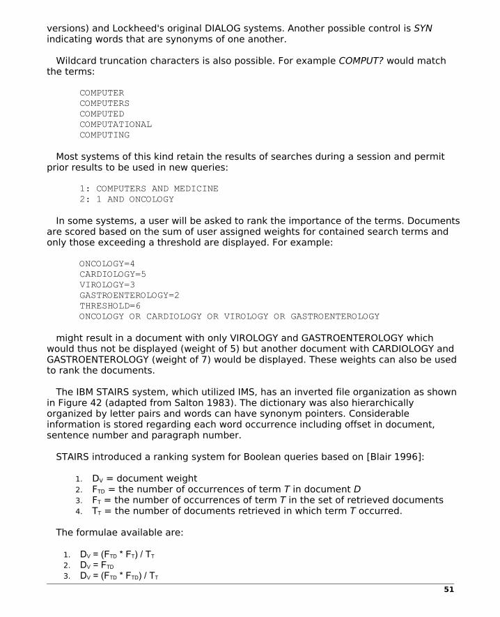
versions) and Lockheed's original DIALOG systems. Another possible control is SYN indicating words that are synonyms of one another.

Wildcard truncation characters is also possible. For example COMPUT? would match the terms:

COMPUTER COMPUTERS COMPUTED COMPUTATIONAL COMPUTING

Most systems of this kind retain the results of searches during a session and permit prior results to be used in new queries:

1: COMPUTERS AND MEDICINE 2: 1 AND ONCOLOGY

In some systems, a user will be asked to rank the importance of the terms. Documents are scored based on the sum of user assigned weights for contained search terms and only those exceeding a threshold are displayed. For example:

ONCOLOGY=4 CARDIOLOGY=5 VIROLOGY=3 GASTROENTEROLOGY=2 THRESHOLD=6 ONCOLOGY OR CARDIOLOGY OR VIROLOGY OR GASTROENTEROLOGY

might result in a document with only VIROLOGY and GASTROENTEROLOGY which would thus not be displayed (weight of 5) but another document with CARDIOLOGY and GASTROENTEROLOGY (weight of 7) would be displayed. These weights can also be used to rank the documents.

The IBM STAIRS system, which utilized IMS, has an inverted file organization as shown in Figure 42 (adapted from Salton 1983). The dictionary was also hierarchically organized by letter pairs and words can have synonym pointers. Considerable information is stored regarding each word occurrence including offset in document, sentence number and paragraph number.

STAIRS introduced a ranking system for Boolean queries based on [Blair 1996]:

1. DV = document weight 2. FTD = the number of occurrences of term T in document D 3. FT = the number of occurrences of term T in the set of retrieved documents4. TT = the number of documents retrieved in which term T occurred.

The formulae available are:

1. DV = (FTD * FT) / TT

2. DV = FTD

3. DV = (FTD * FTD) / TT

51

4. DV = (FTD * FT) / ( TT + TT )5. DV = (FTD * TT) / (FT - FTD )

Figure 42 STAIRS file organization

One of the more well known and largest of the early systems was MEDLARS offered by the National Library of Medicine (NLM). MEDLARS (also known as MEDLINE and now known as PubMed). MEDLARS was initially an automated index on Index Medicus and was accessible via telex at medical libraries. It was a controlled vocabulary system the descendant of which today is MeSH.

The program in Figure 43 is a simple full-text, sequential boolean search written in Mumps.

1 #!/usr/bin/mumps2 3 # boolean.mps Feb 2, 20104 5 again

52

6 7 read !,"Enter query: ",query8 9 do $zwi(query)10 set exp=""11 for w=$zwp do12 . if w="" break13 . if $find("()",w) set exp=exp_w continue14 . if w="|"!(w="OR") set exp=exp_"!" continue15 . if w="~"!(w="NOT") set exp=exp_"'" continue16 . if w="&"!(w="AND") set exp=exp_"&" continue17 . set exp=exp_"$f(line,"""_w_""")"18 19 write !,"Mumps expression to be evaluated on the data set: ",exp,!!20 21 set $noerr=1 // turns off error messages22 set line=" " set i=@exp // test trial of the expression23 if $noerr<0 write "Expression error number ",-$noerror,! goto again24 25 open 1:"translated.txt,old"26 if '$test write "file error",! halt27 open 2:"osu.medline,old"28 if '$test write "file error",! halt29 set i=030 for do31 . use 132 . read line33 . if '$test break34 . set i=i+135 . if @exp do36 .. set off=$p(line," ",2)37 .. set docnbr=$p(line," ",3)38 .. use 239 .. do $zseek(off)40 .. for read title if $p(title," ",1)="TI" quit41 .. use 542 .. write docnbr,?10,$e(title,7,99),!43 44 use 545 write !,i," documents searched",!!

Figure 43 Boolean search in Mumps

The program in Figure 43 produces output such as shown in Figure 44. It operates on the modified OHSUMED database translated.txt an example of which was shown in Figure 13 on page 22 as well as the original OHSUMED dataset osu.medline as depicted in Figure 12 on page 21.

The program first reads a query (line 7) and then loads it into a Mumps buffer (line 9). The query is one or more keywords separated by the operators AND (&), OR (!), NOT ('), and matching sets of parentheses such as:

(term1 & term 2) | (term3 & term4) & ~ term5

(term1 AND term 2) OR (term3 AND term4) AND NOT term5

where term1,...term5 are words.

The loop on lines 12 through 17 extracts tokens ($zwp) from the query and builds a Mumps expression in the string variable exp. This expression is a Mumps translation of

53

the users Boolean query using the Mumps $find() function. So, for example, a user expression such as:

(apples AND oranges) OR pears

becomes:

($find(line,"apples")&$find(line,"oranges"))!$find(line,"pears")

The Mumps expression searches the contents of line for an instance of the keyword (for example, apples). If the keyword is found the result is true (non-zero), false (zero) otherwise. The results of the searches are combined with the logical operators to find a final result (true or false). This result will determine if a document meets the search criteria.

Once the user query is converted to a Mumps rendering, the syntax is tested (lines 22 through 23). The expression is then applied to input from translated.txt in the loop on lines 30 through 42. Each line of translated.txt, read into the Mumps variable line, contains the full text of the original abstract converted to lower case, stemmed, and devoid of punctuation.

The loop reads a line (into the variable line) from translated.txt and executes the expression in exp as the argument of the if statement on line 35. If the expression results in true, the program extracts from line the offset of the document in the original file (line 36) and the document number (line 37). The original document is then read and its title is located and displayed.

Enter query: drink & alcohol

Mumps expression to be evaluated on the data set: $f(line,"drink")&$f(line,"alcohol")

4 Drinkwatchers--description of subjects and evaluation of laboratory markers of heavy 7 Bias in a survey of drinking habits.1490 Self-report validity issues.1491 A comparison of black and white women entering alcoholism treatment.1492 Predictors of attrition from an outpatient alcoholism treatment program for couples.1493 Effect of a change in drinking pattern on the cognitive function of female social 1494 Alcoholic beverage preference as a public statement: self-concept and social image 1496 Influence of tryptophan availability on selection of alcohol and water by men.1497 Alcohol-related problems of children of heavy-drinking parents.1499 Extroversion, anxiety and the perceived effects of alcohol.2024 Psychiatric disorder in medical in-patients.

3648 documents searched

-----

Enter query: (drink | alcohol) & problem

Mumps expression to be evaluated on the data set: ($f(line,"drink")!$f(line,"alcohol"))&$f(line,"problem")

7 Bias in a survey of drinking habits.1056 Reduction of adverse drug reactions by computerized drug interaction screening.1069 Suicide attempts in antisocial alcoholics.1487 Childhood problem behavior and neuropsychological functioning in persons at risk for 1496 Influence of tryptophan availability on selection of alcohol and water by men.1497 Alcohol-related problems of children of heavy-drinking parents.1959 Native American postneonatal mortality.

54

2024 Psychiatric disorder in medical in-patients.

3648 documents searched

Figure 44 Boolean search results

The program in Figure 43 is slow, however, because it searches each document sequentially. A better way would be to build an inverted index of all significant words (with file offset pointers into the original OHSUMED file) and process the queries against the inverted index.

Another Boolean based query system is ERIC - Education Resources Information Center, begun in 1966. It presently has over 1.3 million bibliographic records. It's web site is:

http://www.eric.ed.gov/

Figure 45 is an example Tymnet ERIC search from 1979.

Also from that time period was the NLM MEDLARS system. In it's current form it is accessible from:

http://gateway.nlm.nih.gov/gw/Cmd

At present, all abstracts are indexed by MeSH keywords. Another access portal to on-line bio-related information (NCBI's PubMed) is:

http://www.ncbi.nlm.nih.gov/sites/entrez

See also the Lexis/Nexus system, founded in 1977, which is said to maintain 30 terabytes of content on 11 mainframes (supported by over 300 midrange UNIX servers and nearly 1,000 Windows NT servers) at its main data center in Miamisburg, Ohio). Lexis is a legal database while Nexus deals with "...content from more than 20,000 global news sources, company & industry intelligence providers, biographical and reference sources, intellectual property records, public records, legislative and regulatory filings and legal materials...." (Wikipedia).

A competitive system is Westlaw a description of whose Boolean query language is at:

http://lawschool.westlaw.com/research/tcref.asp?appflag=4.19

55

Figure 45 1979 Tymnet search

56

6.2 Non-Boolean Searching

Instead of structured Boolean queries, many systems permit natural language queries either phrased specifically as a question or as a statement of concepts that the user wishes to see addressed in the retrieved data set. For example:

Oil production in the Mideast post World War II, volume in barrels by year, and country. Major oil producing regions and relative density for the oil produced.

The text need not be phrased as a question. The retrieval system will attempt to match the query with documents in the data base based on the relative importance of the terms in the query and the documents. The match will be based on statistical or probabilistic scoring and not Boolean algebra. The resulting documents, therefore, will be ranked with regard to the degree of similarity to the query.

6.3 Multimedia QUERIES

Increasingly there is a need to search non-text databases. These include videos, pictures, and music. The techniques and methods for these areas are only now being developed.

57

7 Measuring Retrieval System Effectiveness

7.1 Precision and Recall

Two important metrics of information storage and retrieval system performance are precision and recall. Precision measures the degree to which the documents retrieved are relevant and recall measures the degree to which the system can retrieve all relevant documents.

For example, if a system responds to a query by retrieving 10 documents from the collection and of these, 8 are relevant and 2 are irrelevant and if the collection actually has 16 relevant documents, we say that the recall is 50% and the precision is 80%. That is, only 50% of the relevant documents were recalled but of those presented, 80% were correct.

For example, suppose there were 10 relevant documents in the collection and the top ten ranked results of a query are shown in Figure 46.

Rank Relevant? Recall Precision

1 yes 0.1 1.0

2 yes 0.2 1.0

3 no 0.2 0.67

4 yes 0.3 0.75

5 yes 0.4 0.80

6 no 0.4 0.67

7 no 0.4 0.57

8 yes 0.5 0.63

9 no 0.5 0.56

10 yes 0.6 0.60

Figure 46 Precision/recall example

In general, as recall increases, precision declines. For example, in the query mentioned in the previous paragraph, if by setting thresholds lower the system responds with 20 documents instead of 10 and if 12 of these are relevant but 8 are not, the recall has increased to 75% but the precision has fallen to 60%.

In most systems, as you lower thresholds and more documents are retrieved, the recall will rise but the precision will decline. In an ideal system, however, as thresholds are lowered, recall increases but precision remains 100%.

Indexing terms effect the precision/recall results. Generally speaking, terms of low frequency tend to increase the precision of a system's responses at the expense of recall as these tend to reference more narrowly defined concepts. On the other hand, terms of high frequency tend to increase recall at the expense of precision as these are often more broadly defined. Identifying those terms which strike a balance is a major goal of any system.

58

Salton [Salton, 1971] used precision-recall graphs similar to the one shown in Figure 47 in order to compare the results of different retrieval experiments. Those experiments which resulted in a slower drop off in precision as recall increases represent improvement in technique.

Figure 47 Precision/recall graph

See also: "Precision and Recall of Five Search Engines for Retrieval of Scholarly Information in the Field of Biotechnology:"

http://www.webology.ir/2005/v2n2/a12.html

59

8 Document Indexing

8.1 Overview - The Big Picture

Figure 48 Overview of basic document indexing

8.2 Vocabularies

Historically, indexing was conducted manually by experts in a subject who read each document and classify it according to content. Increasingly, manual indexing is being

60

overtaken by automated indexing, of the kind performed by search engines such as Bing, Google and other online indexing and information storage and retrieval systems.

In any indexing scheme, there is a distinction between a controlled and uncontrolled vocabulary scheme. A controlled vocabulary indexing scheme is one in which previously agreed upon standardized terms, categories and hierarchies are employed. On the other hand, an uncontrolled vocabulary based system is one that derives these from the text directly.

In a controlled vocabulary based system, subjects are described using the same preferred term each time and place they are indexed, thus ensuring uniformity across user populations and making it easier to find all information about a specific topic during a search. Many controlled vocabularies exist in many specific fields. These take the form of dictionaries, hierarchies, and thesauri which structure the content of the underlying discipline into commonly accepted categories. For the most part, these are constructed and maintained by government agencies (such as the National Library of Medicine in the U.S. or professional societies such as the ACM).

For example, the Association for Computing Machinery Computing Classification System (1998):

http://www.acm.org/about/class/1998/

which is used to classify documents published in computing literature. This system is hierarchical and invites the author or reviewer of a document to place the document under those categories to which the document most specifically applies and at the level in the tree that best corresponds to the generality of the document. For example, consider the extract of the ACM system shown in Figure 49.

Copyright 2005, by the Association for Computing Machinery, Inc. Permission to make digital or hard copies of part or all of this work for personal or classroom use is granted without fee provided that copies are not made or distributed for profit or commercial advantage and that copies bear this notice and the full citation on the first page.

# D.4 OPERATING SYSTEMS (C)

* D.4.0 General * D.4.1 Process Management o Concurrency o Deadlocks o Multiprocessing/multiprogramming/multitasking o Mutual exclusion o Scheduling o Synchronization o Threads NEW! * D.4.2 Storage Management o Allocation/deallocation strategies o Distributed memories o Garbage collection NEW! o Main memory o Secondary storage o Segmentation [**] o Storage hierarchies o Swapping [**] o Virtual memory * D.4.3 File Systems Management (E.5)

61

o Access methods o Directory structures o Distributed file systems o File organization o Maintenance [**] * D.4.4 Communications Management (C.2) o Buffering o Input/output o Message sending o Network communication o Terminal management [**] * D.4.5 Reliability o Backup procedures o Checkpoint/restart o Fault-tolerance o Verification * D.4.6 Security and Protection (K.6.5) o Access controls o Authentication o Cryptographic controls o Information flow controls o Invasive software (e.g., viruses, worms, Trojan horses) o Security kernels [**] o Verification [**] * D.4.7 Organization and Design o Batch processing systems [**] o Distributed systems o Hierarchical design [**] o Interactive systems o Real-time systems and embedded systems * D.4.8 Performance (C.4, D.2.8, I.6) o Measurements o Modeling and prediction o Monitors o Operational analysis o Queueing theory o Simulation o Stochastic analysis * D.4.9 Systems Programs and Utilities o Command and control languages o Linkers [**] o Loaders [**] o Window managers * D.4.m Miscellaneous

Figure 49 ACM classification system

Numerous other examples abound, especially in technical disciplines where nomenclature is precise. For example:

1. MeSH (Medical Subject Headings) noted above for medicine and related fields

http://www.nlm.nih.gov/mesh/meshhome.html

2. International Classification of Diseases - Clinical Modification version 9 (ICD9-CM) and related codes for diagnostic and forensic medicine:

http://icd9cm.chrisendres.com/

62

3. National Library of Medicine Classification Schedule for medically related works

http://wwwcf.nlm.nih.gov/class/OutlineofNLMClassificationSchedule.html

4. for mental disorders:

http://www.psyweb.com/Mdisord/DSM_IV/dsm_iv.html

5. NCI Surveillance Epidemiology and End Results program for cancer related illnesses:

http://seer.cancer.gov/

6. International Union for Pure and Applied Chemistry Names (IUPAC Names) for chemistry Diagnostic and Statistical Manual IV nomenclature:

http://dl.clackamas.cc.or.us/ch106-01/iupac.htm

7. Library of Congress Classification System for a broad classification system for all works:

http://www.loc.gov/catdir/cpso/lcco/lcco.html

8. Structural Classification of Proteins:

http://scop.mrc-lmb.cam.ac.uk/scop/

9. Yahoo's Categorized Guide to the Web:

http://search.yahoo.com/dir

10. Open Directory Project:

http://www.dmoz.org/

11. For a very long list, see American Society of Indexers Thesauri Online:

http://www.asindexing.org/site/thesonet.shtml

In a manually indexed collection that uses a controlled vocabulary, experts trained in the vocabulary read and assign vocabulary or hierarchy codes to the documents. Historically, because of the complexity of the terminology and the expense of conducting online searches, these systems were accessed by trained personnel who intermediated user's needs and expressed them in the precise vocabulary of the discipline. Prior to the advent of the internet, online database searching was expensive and time consuming. In recent years, however, with the advent of ubiquitous internet access and vastly cheaper computer facilities, the end user is more likely to conduct a search directly.

63

Uncontrolled or derived vocabulary systems have been around for many years. These derive their terms directly from the text. Among the earliest forms were biblical concordances such as:

the King James Bible Hebrew and Greek Concordance Index:

http://www.sacrednamebible.com/kjvstrongs/CONINDEX.htm

an alphabetically organized index which references each occurrence of each term in the text;

more secularly, John Bartlett's Familiar Quotations, 10th ed. 1919.

http://www.bartleby.com/100/s0.html

Manual construction of concordances is tedious at best but well suited as a computer application. A computer based uncontrolled or derived vocabulary can be constructed through numerical analysis of word usage in the collection as a whole. On the other hand, controlled vocabularies may also be used in computer based systems with the aid of training sets of documents.

8.3 Basic Dictionary Construction

8.3.1 Basic Dictionary of Stemmed Words Using Mumps

A program to build a basic dictionary of terms using the pre-processed and stemmed input file translated.txt is shown in Figure 50. The file translated.txt, shown in Figure 13 on page 22, is preprocessed text. The words have already been reduced to lower case, punctuation removed.

Mumps provides the following functions for reading and processing words:

1. $zzScan - returns the next token in from the current input unit delimited by whitespace. Words may contain any character. Punctuation is not removed.

2. $zzScanAlnum - returns the next word from the current input unit delimited by whitespace. Words shorter than 3 and longer that 25 characters are ignored and not returned nor are words that begin with digits. Otherwise, punctuation is removed and words are converted to lower case.

3. $zlower(string) - converts the characters in string to lower case.4. $znormal(arg1,[arg2]) - Function converts the word passed as argument 1 to

lower case and removes any embedded punctuation. If a second argument is given, the word is truncated to the length specified by this argument. If no second argument is given , words are truncated to 25 characters if their length exceeds 25 characters.

5. $zNoBlanks(string) - removes all blanks6. $zBlanks(string) - replaces 2 or more instances of blanks with one blank.7. $zstem(string) - returns an word English word stem of the argument. This

function attempts to remove common endings from words and return a linguistic root stem.

1 #!/usr/bin/mumps2 # dictionary.mps February 2, 2010

64

3 4 kill ^dict5 6 for do7 . set word=$zzScan // input from redirected translated.txt8 . if '$test break9 . if $data(^dict(word)) set ^dict(word)=^dict(word)+110 . else set ^dict(word)=111 12 for word=$order(^dict(word)) write ^dict(word)," ",word,!13 halt

Figure 50 List of stemmed terms

The results, sorted by the frequency are at this link:

http://www.cs.uni.edu/~okane/source/ISR/medline.dictionary.sorted.gz

8.3.2 Basic Dictionary of Stemmed Words Using Linux System Programs

Alternative method to build a dictionary would involve writing each word to a file, sorting the file and then counting the number of times each word appears in the result. For example, first modify the program from Figure 50 as shown in Figure 51. This results in each word being written to a line of it's own.

1 #!/usr/bin/mumps2 # dictionary1.mps Jan 27, 20113 4 for do5 . set word=$zzScan // input from redirected translated.txt6 . if '$test break7 . write word,!8 halt

Figure 51 Modified dictionary program

Also needed is the program in Figure 52 which will load the global array ^dict at the end.

1 #!/usr/bin/mumps 2 # dictget.mps Jan 27, 2011 3 4 kill ^dict 5 write $zd,! 6 for do 7 . set f=$zzscan 8 . if '$t break 9 . set w=$zzscan 10 . set ^dict(w)=f

Figure 52 Dictionary load program

Next run the bash commands:

dictionary1.mps < translated.txt | sort | uniq -c | sort -n | dictget.mps

Figure 53 Dictionary construction using Linux programs

In Figure 53, the output of the Mumps program dictionary.mps is piped to be the input to the Linux sort program whose output, in turn, is passed to the Linux uniq program whose output is passed to sort again whose output is ultimately piped to

65

dictget.mps which loads the global array ^dict from the results. The first instance of the sort program groups each instance of each word together onto adjacent lines. The uniq program counts the number of repeating instances and writes out, for each word, the number of repetitions followed by the word. The second instance of the sort program sorts according to number of repetitions. An advantage of this approach is speed due to the efficiency of the system sort and uniq programs. Moreover, Linux will schedule the concurrent tasks onto more than one core on a multi-core CPU thus resulting in parallel execution.

8.4 Zipf's Law

Zipf's Law states that the frequency ordered rank of a term in a document collection times its frequency of occurrence is approximately equal to a constant:

Frequency * rank ~= constant

where Frequency is the total number of times some term k occurs. Rank is the position number of the term when the terms have been sorted by Frequency. That is, the most frequently occurring term is rank 1, the second most frequently occurring term is rank 2 and so forth.

See also:

http://en.wikipedia.org/wiki/Zipf's_law

The unstemmed medical text data base osu.medline as shown in Figure 12 on page 21 was read and separated into words in lower case. A global array vector indexed by the words was created and incremented for each occurrence of each word. Finally, the results were written to a file where each line contained the word count followed by a blank followed by the word. These were sorted then processed by the zipf.mps program shown if Figure 56.

1 reformat.mps < osu.medline | dictionary.mps | sort -nr | zipf.mps > medline.zipf2 3 #!/usr/bin/mumps 4 # reformat.mps January 18, 2011 5 6 set M=$zgetenv("MAXDOCS") 7 if M="" set M=1000 8 9 set D=0 10 11 for do if D>M quit 12 . set o=$ztell read line 13 . if '$test break // no more input 14 . if $extract(line,1,2)="TI" do quit 15 .. set D=D+1,^doc(D)=off,^title(D)=$extract(line,7,256) 16 .. use 5 17 .. write off," ",D," ",$extract(line,7,1023),! 18 .. quit 19 . if $extract(line,1,2)="MH" quit 20 . if $extract(line,1,13)="STAT- MEDLINE" set off=o use 5 write "xxxxx115xxxxx " quit 21 . if $extract(line,1,2)'="AB" quit 22 . write $extract(line,7,1023)," " 23 . for do // for each line of the abstract 24 .. read line 25 .. if '$test break // no more input 26 .. if line="" break

66

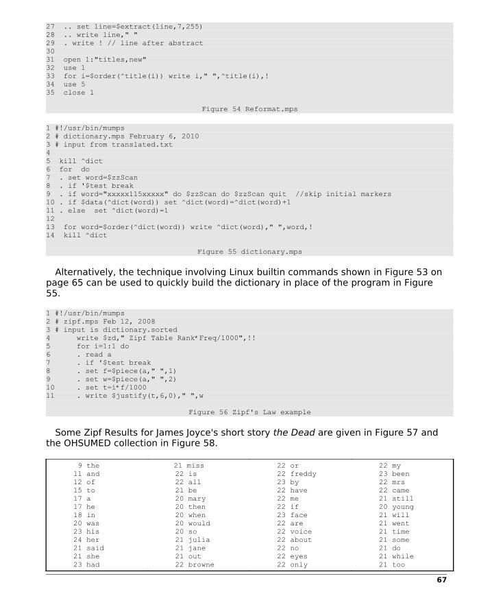
27 .. set line=$extract(line,7,255) 28 .. write line," " 29 . write ! // line after abstract 30 31 open 1:"titles,new" 32 use 1 33 for i=$order(^title(i)) write i," ",^title(i),! 34 use 5 35 close 1

Figure 54 Reformat.mps

1 #!/usr/bin/mumps2 # dictionary.mps February 6, 20103 # input from translated.txt4 5 kill ^dict6 for do7 . set word=$zzScan8 . if '$test break9 . if word="xxxxx115xxxxx" do $zzScan do $zzScan quit //skip initial markers10 . if $data(^dict(word)) set ^dict(word)=^dict(word)+111 . else set ^dict(word)=112 13 for word=$order(^dict(word)) write ^dict(word)," ",word,!14 kill ^dict

Figure 55 dictionary.mps

Alternatively, the technique involving Linux builtin commands shown in Figure 53 on page 65 can be used to quickly build the dictionary in place of the program in Figure 55.

1 #!/usr/bin/mumps2 # zipf.mps Feb 12, 20083 # input is dictionary.sorted4 write $zd," Zipf Table Rank*Freq/1000",!!5 for i=1:1 do6 . read a7 . if '$test break8 . set f=$piece(a," ",1)9 . set w=$piece(a," ",2)10 . set t=i*f/100011 . write $justify(t,6,0)," ",w

Figure 56 Zipf's Law example

Some Zipf Results for James Joyce's short story the Dead are given in Figure 57 and the OHSUMED collection in Figure 58.

9 the 11 and 12 of 15 to 17 a 17 he 18 in 20 was 23 his 24 her 21 said 21 she 23 had

21 miss 22 is 22 all 21 be 20 mary 20 then 20 when 20 would 20 so 21 julia 21 jane 21 out 22 browne

22 or 22 freddy 23 by 22 have 22 me 22 if 23 face 22 are 22 voice 22 about 22 no 22 eyes 22 only

22 my 23 been 22 mrs 22 came 21 still 20 young 21 will 21 went 21 time 21 some 21 do 21 while 21 too

67

23 that 21 gabriel 22 i 22 it 23 with 24 for 24 on 24 him 24 at 23 aunt 24 as 23 you 21 mr 21 but 21 not 21 kate 21 were 21 from 21 they

20 who 21 which 21 what 21 up 22 asked 20 them 21 their 21 one 22 into 21 there 22 malins 22 well 21 like 22 down 22 did 22 o 22 now 21 we 22 very

22 go 21 this 22 its 22 good 22 back 22 an 22 ivors 22 could 22 come 22 over 22 know 22 darcy 22 after 22 where 22 room 22 never 23 ladies 23 gretta 22 old

21 think 21 stood 21 see 21 little 22 how 22 himself 22 again 21 your 21 upon 21 two 22 table 22 snow 22 man 22 long 22 hand 22 before 21 wife 22 why 22 three

Figure 57 Zipf constants - The Dead

369 of 425 in 613 the 733 and 502 a 555 with 561 to 514 the 529 for 426 patients 429 on 462 by 498 is 432 letter 417 was 407 from 425 were 437 an 414 human 365 study 379 we 396 that 393 after 386 as 394 are 396 have 370 cell 381 treatment 393 been

403 during 414 comment 426 has 423 comments 436 see 428 or 437 effects 428 in 425 disease 416 clinical 399 blood 408 at 410 cells 408 effect 417 acute 423 to 408 associated 397 be 400 case 400 studied 396 between 394 renal 389 chronic 383 factor 380 patient 385 who 391 this383 coronary 389 used

393 new 398 protein 403 using 403 use 405 two 411 syndrome 417 therapy 422 report 426 virus 430 growth 434 children 439 role 433 determine 433 rat 422 editorial 420 pulmonary 423 cancer 425 artery 426 an 430 ventricular 435 disease437 response 439 activity 439 normal 435 infection 437 function 442 which 441 studies444 this

447 treated448 not 450 cases 454 immunodeficiency 458 heart 460 myocardial 463 cardiac 465 acid 469 primary 473 following 472 diagnosis 472 receptor 475 analysis 476 management 476 gene 479 carcinoma 479 may 478 we 482 care 484 patients481 liver 484 [news] 486 can 490 effect 493 bone 497 type 497 its 494 had

Figure 58 Zipf constants - OHSUMED

8.5 What are Good Indexing Terms?

Information retrieval pioneer Hans Luhn believed that the resolving power of terms in a collection of text would be greatest in the middle-frequency range. In this context, resolving power is the ability of a term to differentiate between documents relevant and irrelevant to the query. Neither high frequency terms which are spread through many if

68

not all documents nor low frequency terms whose usage is isolated to only a few documents, constitute good indexing terms.

Figure 59 Best indexing terms

In the early days of information retrieval and still to this day when using techniques such Key Word In Context, Key Word Out of Context or Key Word Alongside Context, titles are used to identify content.

1. KWIC: http://en.wikipedia.org/wiki/Key_Word_in_Context2. KWOC: http://nl.wikipedia.org/wiki/KWOC3. KWAC: http://nl.wikipedia.org/wiki/KWAC

However, not all titles are suitable for this form of indexing, however, as this curious link from Amazon.com clearly indicates:

http://www.amazon.com/Books-odd-misleading-titles/lm/1TGJCC3FZ48QY

69

8.5.1 WordNet

WordNet (Miller, George A. "WordNet - About Us." WordNet. Princeton University. 2009:

http://wordnet.princeton.edu)

is:

"... a large lexical database of English, developed under the direction of George A. Miller. Nouns, verbs, adjectives and adverbs are grouped into sets of cognitive synonyms (synsets), each expressing a distinct concept. Synsets are interlinked by means of conceptual-semantic and lexical relations. The resulting network of meaningfully related words and concepts can be navigated with the browser. WordNet is also freely and publicly available for download. WordNet's structure makes it a useful tool for computational linguistics and natural language processing. ..."

One problem confronting all retrieval systems is the ambiguous nature of natural language. While in scientific disciplines there is usually a non-ambiguous, precise vocabulary, in general text, many words have different meanings depending upon context. When we use words to index documents it would be desireable, if possible, to indicate the meaning of the term.

For example, the word base elicits the results in Figure 60 from WordNet

70

Figure 60 WordNet example

Ideally, when processing documents, terms near the term being extracted could be used to disambiguate the context. For example, the sample sentences shown above could provide related terms which could help select the sense of the term.

WordNet can be automatically installed under Ubuntu through the Synaptic Package manager. In command line mode, many aspects of words can be retrieved as shown in Figure 61.

okane@okane-desktop:~/WordNet-3.0$ wn base -synsa

Similarity of adj base

7 senses of base

71

Sense 1basal, base => basic (vs. incidental)

Sense 2base, baseborn, humble, lowly => lowborn (vs. noble)

Sense 3base => inferior (vs. superior)

Sense 4base, immoral => wrong (vs. right)

Sense 5base, mean, meanspirited => ignoble (vs. noble)

Sense 6base, baseborn => illegitimate (vs. legitimate)

Sense 7base => counterfeit (vs. genuine), imitative

Figure 61 WordNet example

Documentation of the command line interface can be found:

http://wordnet.princeton.edu/wordnet/man/wn.1WN.html

8.6 Stop Lists

All indexing techniques need to determine which words or combination of words are the better indexing terms and which terms are poor indications of content. However, in all languages, some words can be eliminated from further consideration immediately based on their frequency of occurrence.

Such a list of words is called a stop list. A stop list is a list of words which are not used for indexing (sometimes referred to as a null dictionary).

For the most part, a stop list is composed of:

1. very high frequency terms conveying no real meaning for purposes of information storage and retrieval (such as: the, and, was, etc.) or,

2. very low frequency words that are one-of-a-kind and unlikely to be important in real world applications. For example, a list of common words in English can be found at:

http://www.webconfs.com/stop-words.php

Once a stop list has been constructed (contained in the file stop.dat in the following examples organized as one word per line), there are two ways to use it in a program.

72

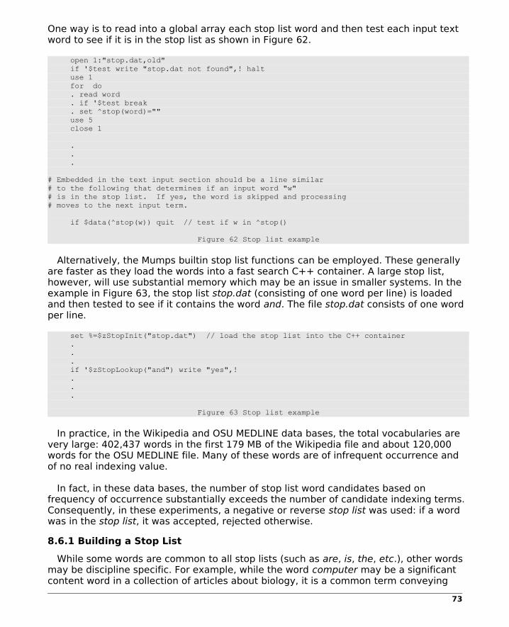
One way is to read into a global array each stop list word and then test each input text word to see if it is in the stop list as shown in Figure 62.

open 1:"stop.dat,old" if '$test write "stop.dat not found",! halt use 1 for do . read word . if '$test break . set ^stop(word)="" use 5 close 1

. . .

# Embedded in the text input section should be a line similar# to the following that determines if an input word "w"# is in the stop list. If yes, the word is skipped and processing# moves to the next input term.

if $data(^stop(w)) quit // test if w in ^stop()

Figure 62 Stop list example

Alternatively, the Mumps builtin stop list functions can be employed. These generally are faster as they load the words into a fast search C++ container. A large stop list, however, will use substantial memory which may be an issue in smaller systems. In the example in Figure 63, the stop list stop.dat (consisting of one word per line) is loaded and then tested to see if it contains the word and. The file stop.dat consists of one word per line.

set %=$zStopInit("stop.dat") // load the stop list into the C++ container . . . if '$zStopLookup("and") write "yes",! . . .

Figure 63 Stop list example

In practice, in the Wikipedia and OSU MEDLINE data bases, the total vocabularies are very large: 402,437 words in the first 179 MB of the Wikipedia file and about 120,000 words for the OSU MEDLINE file. Many of these words are of infrequent occurrence and of no real indexing value.

In fact, in these data bases, the number of stop list word candidates based on frequency of occurrence substantially exceeds the number of candidate indexing terms. Consequently, in these experiments, a negative or reverse stop list was used: if a word was in the stop list, it was accepted, rejected otherwise.

8.6.1 Building a Stop List

While some words are common to all stop lists (such as are, is, the, etc.), other words may be discipline specific. For example, while the word computer may be a significant content word in a collection of articles about biology, it is a common term conveying

73

little content in a collection dealing with computer science. Consequently, it is necessary to examine the vocabulary of each collection to determine which words to include in a stop list in addition to the basic set of words common to all disciplines.

One basic way to build a stop list, is to analyze the frequency of occurrence of words in the text and eliminate words of very high and very low frequency. To do this, we build a program to generate word usage statistics on word usage in the data bases.

For example,the OSU MEDLINE data base word frequency list, sorted in descending frequency of occurrence is

http://www.cs.uni.edu/~okane/source/ISR/medline.dictionary.sorted.gz.

This was created using the translated.txt file.

The command to sort the unordered dictionary was of the form:

sort --reverse --numeric-sort dictionary.unsorted > dictionary.sorted

For the OSU MEDLINE collection, the total number of documents was 293,857 and the total vocabulary consisted of about 120,000 words after stemming, rejection of words less than three or longer than 25 characters in length, and words beginning with numbers. A small number of words have very high frequencies of occurrence compared to the remainder of the file. At the low end of the frequency spectrum, there were about 72,000 words that occurred 5 or fewer times (60% of the total number of words). Figure 64 gives a graph of overall word usage in the OHSUMED collection.

74

Figure 64 Frequency of top 75 OSUMED words

If we were to eliminate words with total frequency of occurrence of 5 or less and greater than 40,000 (the top ranking 101 words), this would result in a candidate vocabulary of about 64,000 words.

For the Wikipedia data base, the vocabulary is very large. In the 179 MB sample used, there were 402,347 distinct words after stemming, rejection of word whose length was less than three or greater than 25, and rejection of words beginning with digits. The full Wikipedia dictionary is

http://www.cs.uni.edu/~okane/source/ISR/wiki.dictionary.sorted.gz

75

Figure 65 Frequency of top 75 Wikipedia words

Figure 65 gives the frequency of the 75 most frequently occurring Wikipedia words. A very small number of words have very high frequencies of occurrence.

76

9 Vector Space Model

9.1 Overview

One popular approach to automatic document indexing, the vector space model, views computer generated document vectors as describing a hyperspace in which the number of dimensions (axes) is equal to the number of indexing terms. This approach was originally proposed by G. Salton:

1. Salton, G.; McGill, M.J., Introduction to Modern Information Retrieval, New York: McGraw Hill; 1983.

2. Salton, G., The state of retrieval system evaluation, Information Processing & Management, 28(4): 441-449; 1992.

3. Videos of a conference on Salton's work and on SMART are available at:

http://www.open-video.org/details.php?videoid=7053

Each document vector is a point in that space defined by the distance along the axis associated with each document term proportional to the term's importance or significance in the document being represented. Queries are also portrayed as vectors that define points in the document hyperspace. Documents whose points in the hyperspace lie within an adjustable envelope of distance from the query vector point are retrieved. The information storage and retrieval process involves converting user typed queries to query vectors and correlating these with document vectors in order to select and rank documents for presentation to the user.

Most IS&R systems have been implemented in C, Pascal and C++, although these languages provide little native support for the hyperspace model. Similarly, popular off-the-shelf legacy relational data base systems are inadequate to efficiently represent or manipulate sparse document vectors in the manner needed to effectively implement IR systems.

77

Figure 66 Vector space model

Documents are viewed as points in a hyperspace whose axes are the terms used in the document vectors. The location of a document in the space is determined by the degree to which the terms are present in a document. Some terms occur several times while other occur not at all. Terms also have weights associated with their content indicating strength and this is factored into the equation as well.

Figure 67 Vector space queries

78

Query vectors are also treated as points in the hyperspace and the documents that lie within a set distance of the query are determined to satisfy the query.

Figure 68 Vector space clustering

Clustering involves identifying groupings of documents and constructing a cluster centroid vector to speed information storage and retrieval. Hierarchies of clusters can also be constructed.

Figure 69 Vector space similarities

79

9.2 Basic Similarity Functions

There are several formulae to calculate the distance between points in the hyperspace. One of the better known is the Cosine function illustrated in the figure above (from Salton 1983). In this formula, the Cosine between points is used to measure the distance. Some of the formulae are:

Sim1Doc i , Doc j =

2[∑k=1

t

Termik⋅Term jk ]

∑k=1

t

Termik∑k=1

t

Term jk

Sim2Doci , Doc j =∑k=1

t

Termik⋅Term jk

∑k=1

t

Termik∑k=1

t

Term jk−∑k=1

t

Termik⋅Term jk

Sim3Doci , Doc j=∑k=1

t

Termik⋅Term jk

∑k=1

t

Termik2⋅∑k=1

t

Term jk2

Sim4 Doci , Doc j=∑k=1

t

Termik⋅Term jk

min∑k=1

t

Termik ,∑k=1

t

Term jk

Sim5Doc i , Doc j =∑k=1

t

minTermik ,Term jk

∑k=1

t

Termik

Figure 70 Similarity functions

80

In the above from (Salton 1983), the Cosine is formula 3. These formulae calculate the similarity between Doci and Docj by examining the relationships between termi,k and

termj,k where termi,k is the weight of term k in document i and termj,k is the weight of

term k in document j. Sim1 is known as the Dice coefficient and Sim2 is known as the

Jaccard coefficient (see: Jaccard 1912, "The distribution of the flora of the alpine zone", New Phytologist 11:37-50).

The following example illustrates the application of the above (from Salton 1983, pg 202-203):

Doci = (3,2,1,0,0,0,1,1)

Docj = (1,1,1,0,0,1,0,0)

Sim1(Doci,Docj)= (2*6)/(8+4) ­> 1

Sim2(Doci,Docj)= (6)/(8+4­6) ­> 1

Sim3(Doci,Docj)= (6)/SQRT(16*4) ­> 0.75 

Sim4(Doci,Docj)= 6/4 ­>  1.5

Sim5(Doci,Docj)= 3/8 ­>  0.375

Figure 71 Example similarity coefficient calculations

9.3 Other Similarity Functions

See Sam's String Metrics:

http://staffwww.dcs.shef.ac.uk/people/S.Chapman/stringmetrics.html

for a discussion of:

Hamming distance Levenshtein distance Needleman-Wunch distance or Sellers Algorithm Smith-Waterman distance Gotoh Distance or Smith-Waterman-Gotoh distance Block distance or L1 distance or City block distance Monge Elkan distance Jaro distance metric Jaro Winkler SoundEx distance metric Matching Coefficient Dice.s Coefficient Jaccard Similarity or Jaccard Coefficient or Tanimoto coefficient Overlap Coefficient Euclidean distance or L2 distance Cosine similarity Variational distance Hellinger distance or Bhattacharyya distance Information Radius (Jensen-Shannon divergence) Harmonic Mean Skew divergence Confusion Probability Tau

81

Fellegi and Sunters (SFS) metric TFIDF or TF/IDF FastA BlastP Maximal matches q-gram Ukkonen Algorithms

82

10 Document-Term Matrix

10.1 Building a Document-Term Matrix

The basic data structure of the Vector Space model is the document-term matrix. That is, a matrix each of whose rows represents a document and each of whose columns represents a word or term in the vocabulary. The elements of the matrix are either the raw number of times a word occurs in a document or a weighted word occurrence. The example in Figure 72 builds a basic word-count document-term matrix from the translated.txt file (see Figure 13 on page 22). The program constructs the following disk resident global arrays:

1. the document-term matrix ^doc(docNbr,word) giving the number of times the term word occurs in document docNbr.

2. a dictionary vector ^dict(word) giving the number of times term word occurs in the total collection.

3. a document frequency vector ^df(word)giving the number of documents term word occurs in the collection.

4. a one element vector ^DocCount(1) giving the total number of documents in the collection.

1 #!/usr/bin/mumps2  # doc­term.mps March 1, 20113 4    kill ^df,^dict,^doc5 6    set min=$zgetenv("MINWORDFREQ") if min="" set min=57    set max=$zgetenv("MAXWORDFREQ") if max="" set max=10008 9    open 1:"translated.txt,old" if '$test write "file not found",! halt10 11 # build doc­term and dictionary 12 13   for  do14   . use 115   . set word=$zzScan if '$test break16   . if word="xxxxx115xxxxx" set off=$zzScan,doc=$zzScan,^doc(doc)=off quit17   . if $data(^doc(doc,word)) set ^doc(doc,word)=^doc(doc,word)+118   . else  set ^doc(doc,word)=119   . if $data(^dict(word)) set ^dict(word)=^dict(word)+120   . else  set ^dict(word)=121 22   use 5 close 123 24 # delete low/high frequency words25 26   for w=$order(^dict(w)) do27   . if ^dict(w)<min!(^dict(w)>max) do28   .. kill ^dict(w)29   .. for d=$order(^doc(d)) if $data(^doc(d,w)) kill ^doc(d,w)30 31 # store number of documents32 33   set ^DocCount(1)=doc34 35 # calculate document frequencies36 37   for d=$order(^doc(d)) do38   . for w=$order(^doc(d,w)) do

83

39   .. if $data(^df(w)) set ^df(w)=^df(w)+140   .. else  set ^df(w)=141 42 # display doc­term matrix43 44   open 1:"doc­term.txt,new"45   use 146 47   for d=$order(^doc(d)) do48   . write "Doc ",d,!49   . set i=050   . for w=$order(^doc(d,w)) write w," (",^doc(d,w),") " set i=i+1 write:i#10=7 !51   . write !!52 53   close 154 55 # display dictionary56 57   open 1:"dictionary.txt,new"58   use 159 60   for w=$order(^dict(w)) write ^dict(w)," ",w,!61 62   close 163 64 # display document frequency vector65 66   open 1:"docfreq.txt,new"67   use 168 69   for w=$order(^df(w)) write ^df(w)," ",w,!70 71   close 172 73   halt

Figure 72 Basic document-term matrix construction

In the example in Figure 72, the translated.txt file is read word by word. The code xxxxx115xxxxx signals the beginning of a new abstract and is followed immediately by the offset of the document in the original file (off) and the document number (doc). The offset in the orginal file of the original text is stored at node^doc(doc) for future reference.

The program checks if word is already in the row for document doc and increments the count if it is, instantiates it to 1 otherwise. Similarly, the count of the total number of times the word has occurred in the collection is stored in ^dict(word).

After the input file has been processed, the total number of times each word has occurred is examined. Words that are too few or many are deleted and their references from the ^doc() matrix are also deleted (lines 26-29).

The total number of documents is stored in ^DocCount(1) (line 33) for future reference.

Next, the number of documents each word occurs in is calculated and stored in the vector ^df(word) (lines 37-40). Then the results are written to three output files.

84

10.2 Assigning Word Weights

Words used for indexing vary in their ability to indicate content and, thus, their importance as indexing terms. Some words, such as the, and, was and so forth are worthless as content indications and we eliminate them from consideration immediately. Other words occur so infrequently that they are also unlikely to be useful as indexing terms. Other words, however, with middle frequency of occurrence are candidates as indexing terms.

However, not all words a equally good index terms. For example, the word computer in a collection of computer science articles conveys very little information useful to indexing the document since so many, if not all, the documents contain the word. The goal here is to determine a metric of the ability of a word to convey information.

In the following example, several weighting schemes are compared. In the example, ^doc(i,w) is the number of times term w occurs in document i; ^dict(w) is the number of times term w occurs in the collection as a whole; ^df(w) is the number of documents term w occurs in; NbrDocs is the total number of documents in the collection; and the function $zlog() is the natural logarithm. The operation "\" is integer division.

Normalize [normal.mps] Sun Dec 15 13:08:59 2002

1000 documents; 29942 word instances, 563 distinct words

^doc(i,w)          Number times word w used in document i^dict(w)           Number times word w used in total collection^df(w)             Number of documents word w appears inWgt1               ^doc(i,w)/(^dict(w)/^df(w))Wgt2               ^doc(i,w)*$zlog(NbrDocs/^df(w))+1Wgt3               Wgt1*Wgt2+0.5\1

Word                   ^doc(i,w) ^dict(w) ^df(w)    Wgt1       Wgt2    Wgt3      MCA

[1]    Death of a cult. (Apple Computer needs to alter its strategy) (column)

apple                        4       261   112     1.716       9.757  17      ­1.1625computer                     4       706   358     2.028       5.109  10     ­19.4405mac                          2       146    71     0.973       6.290   6      ­0.0256macintosh                    4       210   107     2.038       9.940  20      ­0.5855strategy                     2        79    67     1.696       6.406  11      ­0.0592

[2]    Next year in Xanadu. (Ted Nelson's hypertext implementations) Swaine, Michael.

document                     3       114    68     1.789       9.065  16       0.0054operate                      3       269   184     2.052       6.078  12      ­2.1852

[3]    WordPerfect. (WordPerfect for the Macintosh 2.0) (evaluation) Taub, Eric.

edit                         2       111    77     1.387       6.128   8      ­0.0961frame                        2         9     7     1.556      10.924  17       0.0131import                       2        29    19     1.310       8.927  12       0.0998macintosh                    3       210   107     1.529       7.705  12      ­0.5855macro                        3        38    24     1.895      12.189  23       0.1075outstand                     1        10     9     0.900       5.711   5       0.0168user                         4       861   435     2.021       4.330   9     ­26.8094wordperfect                  8        24     8     2.667      39.627  106       0.1747

[4]    Radius Pivot for Built­In Video an Radius Color Pivot. (Hardware Review) (new Mac monitors)(includes related article on design of

85

built­in                     3        35    29     2.486      11.621  29       0.0678color                        3        81    47     1.741      10.173  18       0.0809mac                          2       146    71     0.973       6.290   6      ­0.0256monitor                      6        88    52     3.545      18.739  66       0.0946resolution                   2        50    32     1.280       7.884  10       0.0288screen                       2        92    62     1.348       6.561   9       0.0199video                        4       106    61     2.302      12.188  28       0.0187

[5]    CrystalPrint Express. (Software Review) (high­speed desktop laser printer) (evaluation)

desk                         2       127    76     1.197       6.154   7      ­0.1062engine                       1        15    13     0.867       5.343   5       0.0282font                         4       111    37     1.333      14.187  19       0.6350laser                        3        61    27     1.328      11.836  16       0.2562print                        3       140    66     1.414       9.154  13       0.0509

[6]    4D Write, 4D Calc, 4D XREF. (Software Review) (add­ins for Acius' Fourth Dimension database software) (evaluation)

add­in                       2        97    38     0.784       7.540   6       0.5551analysis                     2       179   139     1.553       4.947   8      ­0.8492database                     5       138    67     2.428      14.515  35       0.1832midrange                     1         7     6     0.857       6.116   5       0.0218spreadsheet                  2        75    44     1.173       7.247   9       0.1707vary                         1         7     6     0.857       6.116   5       0.0107

[7]    ConvertIt! (Software Review) (utility for converting HyperCard stacks to IBM PC format) (evaluation)

converter                    2        24    13     1.083       9.686  10       0.0698doe                          5        97    84     4.330      13.385  58      ­0.1139graphical                    2       307   171     1.114       4.532   5      ­2.4079hypercard                    4        25    13     2.080      18.371  38       0.1517mac                          2       146    71     0.973       6.290   6      ­0.0256map                          2        17    10     1.176      10.210  12       0.1180program                      4       670   334     1.994       5.386  11     ­15.4832script                       3        54    32     1.778      11.326  20       0.1239software                     3       913   449     1.475       3.402   5     ­30.7596stack                        5        15     8     2.667      25.142  67       0.0700

[8]    Reports 2.0. (Software Review) (Nine To Five Software Reports 2.0 report generator for HyperCard 2.0) (evaluation)

hypercard                    5        25    13     2.600      22.714  59       0.1517print                        3       140    66     1.414       9.154  13       0.0509software                     3       913   449     1.475       3.402   5     ­30.7596stack                        2        15     8     1.067      10.657  11       0.0700

[9]    Project­scheduling tools. (FastTrack Schedule, MacSchedule) (Software Review) (evaluation)

manage                       2       318   174     1.094       4.497   5      ­2.4884

[10]   Digital Darkroom. (Software Review) (new version of image­processing software) (evaluation)

apply                        1        17    15     0.882       5.200   5       0.0317digital                      4        90    52     2.311      12.826  30      ­0.0042image                        4       107    58     2.168      12.389  27       0.1422palette                      2        18    12     1.333       9.846  13       0.0660portion                      2        17    15     1.765       9.399  17       0.0295software                     4       913   449     1.967       4.203   8     ­30.7596text                         2        55    46     1.673       7.158  12       0.0304user                         5       861   435     2.526       5.162  13     ­26.8094

86

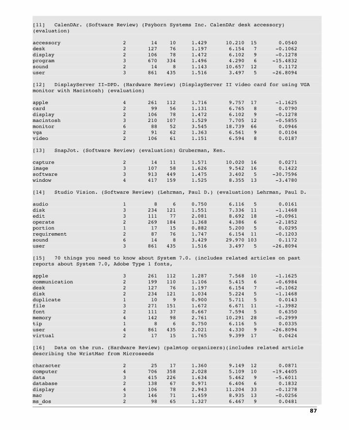
[11]   CalenDAr. (Software Review) (Psyborn Systems Inc. CalenDAr desk accessory) (evaluation)

accessory                    2        14    10     1.429      10.210  15       0.0540desk                         2       127    76     1.197       6.154   7      ­0.1062display                      2       106    78     1.472       6.102   9      ­0.1278program                      3       670   334     1.496       4.290   6     ­15.4832sound                        2        14     8     1.143      10.657  12       0.1172user                         3       861   435     1.516       3.497   5     ­26.8094

[12]   DisplayServer II­DPD. (Hardware Review) (DisplayServer II video card for using VGA monitor with Macintosh) (evaluation)

apple                        4       261   112     1.716       9.757  17      ­1.1625card                         2        99    56     1.131       6.765   8       0.0790display                      2       106    78     1.472       6.102   9      ­0.1278macintosh                    3       210   107     1.529       7.705  12      ­0.5855monitor                      6        88    52     3.545      18.739  66       0.0946vga                          2        91    62     1.363       6.561   9       0.0104video                        2       106    61     1.151       6.594   8       0.0187

[13]   SnapJot. (Software Review) (evaluation) Gruberman, Ken.

capture                      2        14    11     1.571      10.020  16       0.0271image                        3       107    58     1.626       9.542  16       0.1422software                     3       913   449     1.475       3.402   5     ­30.7596window                       4       417   159     1.525       8.355  13      ­3.4780

[14]   Studio Vision. (Software Review) (Lehrman, Paul D.) (evaluation) Lehrman, Paul D.

audio                        1         8     6     0.750       6.116   5       0.0161disk                         3       234   121     1.551       7.336  11      ­1.1468edit                         3       111    77     2.081       8.692  18      ­0.0961operate                      2       269   184     1.368       4.386   6      ­2.1852portion                      1        17    15     0.882       5.200   5       0.0295requirement                  2        87    76     1.747       6.154  11      ­0.1203sound                        6        14     8     3.429      29.970 103       0.1172user                         3       861   435     1.516       3.497   5     ­26.8094

[15]   70 things you need to know about System 7.0. (includes related articles on past reports about System 7.0, Adobe Type 1 fonts,

apple                        3       261   112     1.287       7.568  10      ­1.1625communication                2       199   110     1.106       5.415   6      ­0.6984desk                         2       127    76     1.197       6.154   7      ­0.1062disk                         2       234   121     1.034       5.224   5      ­1.1468duplicate                    1        10     9     0.900       5.711   5       0.0143file                         3       271   151     1.672       6.671  11      ­1.3982font                         2       111    37     0.667       7.594   5       0.6350memory                       4       142    98     2.761      10.291  28      ­0.2999tip                          1         8     6     0.750       6.116   5       0.0335user                         4       861   435     2.021       4.330   9     ­26.8094virtual                      2        17    15     1.765       9.399  17       0.0424

[16]   Data on the run. (Hardware Review) (palmtop organizers)(includes related article describing the WristMac from Microseeds

character                    2        25    17     1.360       9.149  12       0.0871computer                     4       706   358     2.028       5.109  10     ­19.4405data                         3       415   226     1.634       5.462   9      ­5.6011database                     2       138    67     0.971       6.406   6       0.1832display                      4       106    78     2.943      11.204  33      ­0.1278mac                          3       146    71     1.459       8.935  13      ­0.0256ms_dos                       2        98    65     1.327       6.467   9       0.0481

87

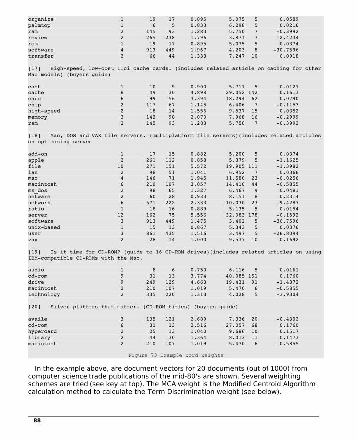
organize                     1        19    17     0.895       5.075   5       0.0589palmtop                      1         6     5     0.833       6.298   5       0.0216ram                          2       145    93     1.283       5.750   7      ­0.3992review                       2       265   238     1.796       3.871   7      ­2.4234rom                          1        19    17     0.895       5.075   5       0.0374software                     4       913   449     1.967       4.203   8     ­30.7596transfer                     2        66    44     1.333       7.247  10       0.0918

[17]   High­speed, low­cost IIci cache cards. (includes related article on caching for other Mac models) (buyers guide)

cach                         1        10     9     0.900       5.711   5       0.0127cache                        8        49    30     4.898      29.052 142       0.1613card                         6        99    56     3.394      18.294  62       0.0790chip                         2       117    67     1.145       6.406   7      ­0.1153high­speed                   2        18    14     1.556       9.537  15       0.0352memory                       3       142    98     2.070       7.968  16      ­0.2999ram                          2       145    93     1.283       5.750   7      ­0.3992

[18]   Mac, DOS and VAX file servers. (multiplatform file servers)(includes related articles on optimizing server

add­on                       1        17    15     0.882       5.200   5       0.0374apple                        2       261   112     0.858       5.379   5      ­1.1625file                        10       271   151     5.572      19.905 111      ­1.3982lan                          2        98    51     1.041       6.952   7       0.0366mac                          4       146    71     1.945      11.580  23      ­0.0256macintosh                    6       210   107     3.057      14.410  44      ­0.5855ms_dos                       2        98    65     1.327       6.467   9       0.0481netware                      2        60    28     0.933       8.151   8       0.2314network                      6       571   222     2.333      10.030  23      ­9.4287ratio                        1        18    16     0.889       5.135   5       0.0154server                      12       162    75     5.556      32.083 178      ­0.1592software                     3       913   449     1.475       3.402   5     ­30.7596unix­based                   1        15    13     0.867       5.343   5       0.0376user                         3       861   435     1.516       3.497   5     ­26.8094vax                          2        28    14     1.000       9.537  10       0.1692

[19]   Is it time for CD­ROM? (guide to 16 CD­ROM drives)(includes related articles on using IBM­compatible CD­ROMs with the Mac,

audio                        1         8     6     0.750       6.116   5       0.0161cd­rom                       9        31    13     3.774      40.085 151       0.1760drive                        9       249   129     4.663      19.431  91      ­1.4872macintosh                    2       210   107     1.019       5.470   6      ­0.5855technology                   2       335   220     1.313       4.028   5      ­3.9304

[20]   Silver platters that matter. (CD­ROM titles) (buyers guide)

availe                       3       135   121     2.689       7.336  20      ­0.4302cd­rom                       6        31    13     2.516      27.057  68       0.1760hypercard                    2        25    13     1.040       9.686  10       0.1517library                      2        44    30     1.364       8.013  11       0.1473macintosh                    2       210   107     1.019       5.470   6      ­0.5855

Figure 73 Example word weights

In the example above, are document vectors for 20 documents (out of 1000) from computer science trade publications of the mid-80's are shown. Several weighting schemes are tried (see key at top). The MCA weight is the Modified Centroid Algorithm calculation method to calculate the Term Discrimination weight (see below).

88

10.3 Inverse Document Frequency Weight

One of the simplest word weight schemes to implement is the Inverse Document Frequency weight. The IDF weight is the measure of how widely distributed a term is in a collection. Low IDF weights mean that the term is widely used while high weights indicate that the usage is more concentrated.

The IDF weight measures the weight of a term in the collection as a whole, rather than the weight of a term in a document.

In individual document vectors, the normalized frequency of occurrence of each term is multiplied by the IDF to give a weight for the term in the particular document. Thus, a term with a high frequency but a low IDF weight could still be a highly weighted term in a particular document, and, on the other hand, a term with a low frequency but a high IDF weight could also be an important term in a given document. The IDF weight for a term W in a collection of N documents is:

log2N

DocFreqw

where DocFreqw is the number of documents in which term W occurs.

10.3.1 OSU MEDLINE Data Base IDF Weights

The IDF weights for the OSU MEDLINE collection were calculated after the words were processed by the stemming function $zstem() and the values are stored in the global array ^df(word) for subsequent use and also printed to standard output. The IDF weights for a recent run on the OSU data base is here:

http://www.cs.uni.edu/~okane/source/ISR/medline.idf.sorted.gz.

Note: due to tuning parameters that set thresholds for the construction of the stop list and other factors, different runs on the data base will produce some variation in the values displayed. The weights range from lows such as:

0.189135 human0.288966 and0.300320 the0.542811 with0.737224 for0.793466 was0.867298 were

to highs such as:

12.590849 actinomycetoma12.590849 actinomycetomata12.590849 actinomycoma12.590849 actinomyosine12.590849 actinoplane12.590849 actinopterygii12.590849 actinoxanthin12.590849 actisomide12.590849 activ12.590849 activationin

89

Note: for a given IDF value, the words are presented alphabetically. The OSU MEDLINE collection has many code words that appear only once.

10.3.2 Wikipedia Data Base IDF Weights

Similarly, the Wikipedia IDF weights were calculated and the results are in:

http://www.cs.uni.edu/~okane/source/ISR/wiki.idf.sorted.gz.

The weights range from lows such as:

1.61 further1.62 either1.63 especial1.65 certain1.65 having1.67 almost1.67 along1.68 involve1.68 receive

to highs such as:

9.87 altopia9.87 alyque9.87 amangkur9.87 amarant9.87 amaranthus9.87 amarantine9.87 amazonite9.87 ambacht9.87 ambiorix

10.3.3 Calculating IDF Weights

Calculating IDF weights involves first building a document-term matrix (^doc(i,w)) where i is the document number and w is a term. Each cell in the document-term matrix will contain the count of the number of times that the term occurs in the document).

Next, from the document-term matrix, construct a document frequency vector (^df(w)) where each element gives the number documents in which the term w occurs.

When the document frequency vector has been built, the individual IDF values for each word can be calculated.

The results of the IDF procedure may be used to enhance the stop list with words that have very low values.

A basic program to create a document-term matrix and calculate IDF weights is shown in Figure 74. It assumes that the global arrays ^doc(), ^dict() and ^df() have been calculated (see Figure 72 on page 84).

1 #!/usr/bin/mumps 2 3  # idf.mps March 1, 2011 4  5    set min=$zgetenv("MINIDF") if min="" set min=5 6 

90

7    open 1:"idf.txt,new" use 18 9    set doc=^DocCount(1)10  11  # calculate IDF weights12 13    for w=$order(^df(w)) do 14   . set x=$zlog(doc/^df(w))15   . if x<min quit16   . set ^idf(w)=$justify(x,1,2)17   . write ^idf(w)," ",w,! 18  19   close 1 use 5 20  21  # weight documents22  23  for d=$order(^doc(d)) do24  . for w=$order(^doc(d,w)) do25  .. if $data(^idf(w)) set ^doc(d,w)=^doc(d,w)*^idf(w)26  .. else  kill ^doc(d,w)27  28  # display weighted doc­term matrix29  30    open 1:"wgted­doc­term.txt,new"31    use 132 33    for d=$order(^doc(d)) do34    . write "Doc ",d,!35    . set i=036    . for w=$order(^doc(d,w)) write w," (",^doc(d,w),") " set i=i+1 write:i#10=7 !37    . write !!38 39    close 140    41    halt 

Figure 74 IDF calculation

Example results can be found here:

http://www.cs.uni.edu/~okane/source/ISR/medline.idf.sorted.gz

http://www.cs.uni.edu/~okane/source/ISR/medline.weighted-doc-vectors.gz

http://www.cs.uni.edu/~okane/source/ISR/medline.weighted-term-vectors.gz

http://www.cs.uni.edu/~okane/source/ISR/wiki.idf.sorted.gz

http://www.cs.uni.edu/~okane/source/ISR/wiki.weighted-doc-vectors.gz

http://www.cs.uni.edu/~okane/source/ISR/wiki.weighted-term-vectors.gz

10.4 Signal-noise ratio (see Salton83 links, pages 63-66)

http://www.cs.uni.edu/~okane/source/ISR/salton83.pdf

10.5 Discrimination Coefficients (pages 66-71) and

Simple Automatic Indexing (pages Salton83, 71-75):

91

http://www.cs.uni.edu/~okane/source/ISR/salton83.pdf

Willett 1985

http://www.cs.uni.edu/~okane/source/ISR/willett85.pdf

Crouch 1988

http://www.cs.uni.edu/~okane/source/ISR/crouch88.pdf

The Term Discrimination factor measures the degree to which a term differentiates one document from another. It is calculated based on the effect a term has on overall hyperspace density with and without a given term. If the space density is greater when a term is removed from consideration, that means the term was making documents look less like one another (a good discriminator) while terms whose remove decreases the density are poor discriminators. The discrimination values for a set of terms are similar to the values for the IDF weights but not exactly.

The basic procedure calls for first calculating the average of pair-wise similarities between all documents in the space. Then for each word, the average of the pair-wise similarities of all the documents is calculated without that word. The difference in the averages is the term discrimination value for the word. When the average similarity increases when a word is removed, the word was a good discriminator - it made documents look less like one another. On the other hand, if the average similarity decreased, the term was not a good discriminator since it made the documents look more like one another. In practice, this is an expensive weight to calculate unless speed-up techniques are used.

The modified centroid algorithm (see Crouch 1987), is an attempt to improve the speed of calculation. The exact calculation, where all pairwise similarity values are calculated each time, is of complexity of the order of (N)(N-1)(w)(W) where N is the number of documents, W is the number of words in the collection and w is the average number of terms per document vector.

Crouch (1988) discusses several methods to speed this calculation. The first of these, the approximate approach, consists of calculating the similarities of the documents with a centroid vector representing the collection as a whole rather that pair-wise. This results in considerable simplification as the number of similarities to be calculated drops from (N)(N-1) to N.

Another modification, called the Modified Centroid Algorithm is based on:

1. Subtracting the original contributions to the sum of the similarities of those documents containing some term W and replacing these values with the similarities calculated between the the centroid and the document vectors with W removed;

2. Storing the original contributions to the total similarity by each document in a vector for later use (rather than recalculating this value); and

92

3. Using an inverted list to identify those documents which contain the indexing terms.

In the centroid approximation of discrimination coefficients, a centroid vector is calculated. A centroid vector is a vector whose individual components are the average usage of each word in the vocabulary. A centroid vector is the average of all the document vectors and, by analogy, is at the center of the hyperspace. When using a centroid vector, rather than calculating all the pair-wise similarities of each document with each other document, the average similarity is calculated by comparing each document with the centroid vector. This improves the performance to a complexity on the order of (N)(w)(W).

As modified centroid algorithm (MCA) calculates the average similarity, it stores the contribution of each document to the total document density (order n space required). When calculating the effect of a term on the document space density, the MCA subtracts the original contribution of those documents that contain the term under consideration and re-adds the document's contribution re-calculated without the contribution of the term under consideration. Complexity is on the order of (DF)(w)(W) where DF is the average number of documents in which a term occurs. Finally, an inverted term-document matrix is used to quickly identify those documents that contain terms of interest rather than scanning through the entire document-term matrix looking for documents containing a given term.

While the MCA method yields values that are only an approximation of the exact method, the values are very similar in most cases and the savings in time to calculate the coefficients is very significant. Crouch (Crouch 1987) reports that the MCA method was on the order of 527 times faster than the exact method on relatively small data sets. Larger data sets yield even greater savings as the time required for the exact method grows with the square of the number of documents while the MCA method grows linearly with the number of documents. The basic MCA algorithm is given in Figure 75.

1 #!/usr/bin/mumps2 3 # discrim4.mps March 5, 20084 5      open 1:"discrim,new"6      use 17 8      set D=^DocCount(1)  // number of documents9      kill ^mca10 11     set t1=$zd112 #++++++++++++++++++++++++++++++++++++++++++++++++++++++++++++++++++++++13 # calculate centroid vector ^c() for entire collection and14 # the sum of the squares (needed in cos calc but should only be done 15 once)16 #++++++++++++++++++++++++++++++++++++++++++++++++++++++++++++++++++++++17 18      for w=$order(^dict(w)) do19      . set ^c(w)=^dict(w)/D   // centroid is composed of avg word usage20 21 #++++++++++++++++++++++++++++++++++++++++++++++++++++++++++++++++++++++22 # Calculate total similarity of docs for all words (T) by23 # calculating sum of the similarities of each document with the centroid.24 # Remember and store contribution of each document in ^dc(dn).25 #++++++++++++++++++++++++++++++++++++++++++++++++++++++++++++++++++++++

93

26 27      set T=028      for i=$order(^doc(i)) do29      . set cos=$zzCosine(^doc(i),^c)30      . set ^dc(i)=cos           // save contributions to total of each31      . set T=cos+T              // sum the cosines32 33 #++++++++++++++++++++++++++++++++++++++++++++++++++++++++++++++++++++++34 # calculate similarity of doc space with words removed35 #++++++++++++++++++++++++++++++++++++++++++++++++++++++++++++++++++++++36 37      for W=$order(^dict(W)) do  // for each word W38 39 #++++++++++++++++++++++++++++++++++++++++++++++++++++++++++++++++++++++40 # For each document containing W, calculate sum of the contribution41 # of the cosines of these documents to the total (T).  ^dc(i) is42 # the original contribution of doc i. Sum of contributions stored in T143 #++++++++++++++++++++++++++++++++++++++++++++++++++++++++++++++++++++++44 45      . set T1=0,T2=046      . for d=$order(^index(W,d)) do   //for each doc d containing W47      .. set T1=^dc(d)+T1              // sum of orig contribution48      .. kill ^tmp49      .. for w1=$order(^doc(d,w1)) do  // make a copy of ^doc50      ... if w1=W quit                 // don't copy W51      ... set ^tmp(w1)=^doc(d,w1)52      .. set T2=T2+$zzCosine(^tmp,^c)  // sum of cosines without W53 54 #++++++++++++++++++++++++++++++++++++++++++++++++++++++++++++++++++++++55 # calculate the change and shift the results.56 #++++++++++++++++++++++++++++++++++++++++++++++++++++++++++++++++++++++57 58      . set r=T2­T1*10000\159 60      . write r," ",W,!61      . set ^mca(W)=r62 63      use 564      write $zd1­t1,!  // time taken65      close 166      halt

Figure 75 Modified centroid algorithm

In Figure 75, the density of the space without word W is:

(T-T1+T2)

where the original contribution of of the documents that contained word W is T1 which is subtracted from the original density and the contribution of these same documents without word W is T2 which is added to the original density.

The difference between the original density T and the density without word W is:

T-(T-T1+T2)

which reduces to

(T1-T2)

94

A larger T means documents more like one another. Thus, if T1 is larger than T2, it means that with the word W, T is larger than without W and thus the documents more like one another and W is a poor discriminator. Alternatively, if T2 is larger than T1, it means that with the word, the documents are further apart. W is a good discriminator. I

In order to give positive values to good discriminators and negative values to poor discriminators, in Figure 75 we reverse the order of the subtraction to become:

(T2-T1)

In Figure 76 is a further refinement of Figure 75. It stores the sum of the squares of the components of the centroid vector which are needed in the denominator of each cosine calculation thus eliminating this step This version also eliminates the step where a copy is made of the individual document vectors.

Overall, the changes noted above and implemented in the program below can result in substantial time improvement. On a test run on 10,000 abstracts from the MEDLINE database, the procedure above took 2,053 seconds while the one below took 378 seconds.

1 #!/usr/bin/mumps2 3 # discrim3.mps March 5, 20084 5      open 1:"discrim,new"6      use 17 8      set D=^DocCount(1)  // number of documents9      set sq=010      kill ^mca11 12      set t1=$zd113 14 #++++++++++++++++++++++++++++++++++++++++++++++++++++++++++++++++++++++15 # calculate centroid vector ^c() for entire collection and16 # the sum of the squares (needed in cos calc but should only be done 17 once)18 #++++++++++++++++++++++++++++++++++++++++++++++++++++++++++++++++++++++19 20      for w=$order(^dict(w)) do21      . set ^c(w)=^dict(w)/D   // centroid is composed of avg word usage22      . set sq=^c(w)**2+sq     // The sum of the squares is needed below.23 24 #++++++++++++++++++++++++++++++++++++++++++++++++++++++++++++++++++++++25 # Calculate total similarity of doc for all words (T) space by26 # calculating the sum of the similarities of each document with the 27 centroid.28 # Remember and store contribution of each document in ^dc(dn).29 #++++++++++++++++++++++++++++++++++++++++++++++++++++++++++++++++++++++30 31      set T=032      for i=$order(^doc(i)) do33      . set x=034      . set y=035 36      . for w=$order(^doc(i,w)) do37      .. set d=^doc(i,w)38      .. set x=d*^c(w)+x                       // numerator of cos(c,doc) calc39      .. set y=d*d+y                           // part of denominator

95

40 41 #++++++++++++++++++++++++++++++++++++++++++++++++++++++++++++++++++++++42 # Calculate and store the cos(c,doc(i)).43 # Remember in ^dc(i) the contribution that this document made to the 44 total.45 #++++++++++++++++++++++++++++++++++++++++++++++++++++++++++++++++++++++46 47      . if y=0 quit48      . set ^dc(i)=x/$zsqrt(sq*y)              // cos(c,doc(i))49      . set T=^dc(i)+T                         // sum the cosines50 51 #++++++++++++++++++++++++++++++++++++++++++++++++++++++++++++++++++++++52 # calculate similarity of doc space with words removed53 #++++++++++++++++++++++++++++++++++++++++++++++++++++++++++++++++++++++54 55      for W=$order(^dict(W)) do56 57 #++++++++++++++++++++++++++++++++++++++++++++++++++++++++++++++++++++++58 # For each document containing W, calculate sum of the contribution59 # of the cosines of these documents to the total (T).  ^dc(i) is60 # the original contribution of doc i.  Sum of contributions is stored in61 T1.62 #++++++++++++++++++++++++++++++++++++++++++++++++++++++++++++++++++++++63 64      . set T1=0,T2=065      . for i=$order(^index(W,i)) do            // row of doc nbrs for word66      .. set T1=^dc(i)+T1                       // use prevsly calc'd cos67 68 #++++++++++++++++++++++++++++++++++++++++++++++++++++++++++++++++++++++69 # For each word in document i, recalculate cos(c,doc) but without word W70 #++++++++++++++++++++++++++++++++++++++++++++++++++++++++++++++++++++++71 72      .. set x=073      .. set y=074      .. for w=$order(^doc(i,w)) do75      ... if w'=W do                          // if W not w76      .... set d=^doc(i,w)77      .... set x=d*^c(w)+x                   //  d*^c(w)+x78      .... set y=d**2+y79 80      .. if y=0 quit81      .. set T2=x/$zsqrt(sq*y)+T2               // T2 sums cosines without W82 83 #++++++++++++++++++++++++++++++++++++++++++++++++++++++++++++++++++++++84 # subtract original contribution with W (T1) and add contribution85 # without W (T2) and calculate r ­ the change, and store in ^mca(W)86 #++++++++++++++++++++++++++++++++++++++++++++++++++++++++++++++++++++++87 88 #     if old (T1) big and new (T2) small, density declines89 90      . set r=T2­T1*10000\191      . write r," ",^dfi(W)," ",W,!92      . set ^mca(W)=r93 94      use 595      write "Time used: ",$zd1­t1,!96      close 197      halt

Figure 76 Enhanced modified centroid algorithm

Example results:

http://www.cs.uni.edu/~okane/source/ISR/wiki.discrim.sorted.gz

96

http://www.cs.uni.edu/~okane/source/ISR/medline.discrim.sorted.gz

Note: the discrimination coefficients output is in three columns: the first is the coefficient times 10,000, the second is the IDF for the word and the third is the word.

11 Term-Document Matrix

The term-document matrix is a matrix where the rows represent the words and the columns are the documents. The contents of each element is the same as in the document-term matrix: the frequency or weighted frequency of the term in the document.

The term-document matrix is the transpose of the document term matrix and can be calculated in Mumps with the statement:

do $zzTranspose(^doc,^index)

where the result will be in the global array ^index().

http://www.cs.uni.edu/~okane/source/ISR/medline.weighted-term-vectors.gz

11.1 Retrieval Using the Doc-Term Matrix

A simple program to scan the document-term matrix looking for documents that have terms from a query vector is given in Figure 77. (Results based on 20,000 documents).

1 #!/usr/bin/mumps2 # tq.mps Feb 27, 20083 4      kill ^query5      write "Enter search terms: "6      read a7      if a="" halt8      for i=1:1 do9      . set b=$piece(a," ",i)10      . if b="" break11      . set b=$zn(b) // lower case, no punct12      . set b=$zstem(b) // stem it13      . set ^query(b)=""14 15      if $order(^query(""))="" halt16 17      for j=$order(^query(j)) write j,!18 19      set t1=$zd120      for i=$order(^doc(i)) do21      . set f=122      . for j=$order(^query(j)) do23      .. if '$data(^doc(i,j)) set f=0 break24      . if f write i,?8,$extract(^t(i),1,70),!25 26      write !,"Elapsed time: ",$zd1­t1,!

Enter search terms: epithelial fibrosisepithelialfibrosis10001   Phosphorylation fails to activate chloride channels from cystic fibro18197   Relationship between mammographic and histologic features of breast t6944    Cyclic adenosine monophosphate­dependent kinase in cystic fibrosis tr

97

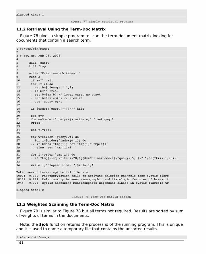
Elapsed time: 1

Figure 77 Simple retrieval program

11.2 Retrieval Using the Term-Doc Matrix

Figure 78 gives a simple program to scan the term-document matrix looking for documents that contain a search term.

1 #!/usr/bin/mumps2 3 # tqw.mps Feb 28, 20084 5      kill ^query6      kill ^tmp7 8      write "Enter search terms: "9      read a10      if a="" halt11      for i=1:1 do12      . set b=$piece(a," ",i)13      . if b="" break14      . set b=$zn(b) // lower case, no punct15      . set b=$zstem(b) // stem it16      . set ^query(b)=117 18      if $order(^query(""))="" halt19 20      set q=021      for w=$order(^query(w)) write w," " set q=q+122      write !23 24      set t1=$zd125 26      for w=$order(^query(w)) do27      . for i=$order(^index(w,i)) do28      .. if $data(^tmp(i)) set ^tmp(i)=^tmp(i)+129      .. else  set ^tmp(i)=130 31      for i=$order(^tmp(i)) do32      . if ^tmp(i)=q write i,?8,$j($zzCosine(^doc(i),^query),5,3)," ",$e(^t(i),1,70),!33 34      write !,"Elapsed time: ",$zd1­t1,!

Enter search terms: epithelial fibrosis10001  0.180  Phosphorylation fails to activate chloride channels from cystic fibro18197  0.291  Relationship between mammographic and histologic features of breast t6944   0.323  Cyclic adenosine monophosphate­dependent kinase in cystic fibrosis tr

Elapsed time: 0

Figure 78 Term-Doc matrix search

11.3 Weighted Scanning the Term-Doc Matrix

Figure 79 is similar to Figure 78 but all terms not required. Results are sorted by sum of weights of terms in the documents.

Note: the $job function returns the process id of the running program. This is unique and it is used to name a temporary file that contains the unsorted results.

1 #!/usr/bin/mumps

98

2 # tqw1.mps Feb 27, 20083 4      kill ^query5      kill ^tmp6 7      write "Enter search terms: "8      read a9      if a="" halt10      for i=1:1 do11      . set b=$piece(a," ",i)12      . if b="" break13      . set b=$zn(b) // lower case, no punct14      . set b=$zstem(b) // stem it15      . set ^query(b)=""16 17      if $order(^query(""))="" halt18 19      set q=020      for w=$order(^query(w)) write w," " set q=q+121      write !22 23      set t1=$zd124 25      for w=$order(^query(w)) do26      . for i=$order(^index(w,i)) do27      .. if $data(^tmp(i)) set ^tmp(i)=^tmp(i)+^index(w,i)28      .. else  set ^tmp(i)=^index(w,i)29 30      set fn=$job_",new"31      open 1:fn  // $job number is unique to this process32      use 133      for i=$order(^tmp(i)) do34      . write ^tmp(i)," ",$extract(^t(i),1,70),!35      close 136      use 537      set %=$zsystem("sort ­n "_$job_"; rm "_$job)38 39      write !,"Elapsed time: ",$zd1­t1,!

Enter search terms: epithelial fibrosis epithelial fibrosis9.02  Adaptation of the jejunal mucosa in the experimental blind loop syndr9.02  Adherence of Staphylococcus aureus to squamous epithelium: role of fi9.02  Anti­Fx1A induces association of Heymann nephritis antigens with micr9.02  Anti­human tumor antibodies induced in mice and rabbits by "internal9.02  Bacterial adherence: the attachment of group A streptococci to mucosa9.02  Benign persistent asymptomatic proteinuria with incomplete foot proce9.02  Binding of navy bean (Phaseolus vulgaris) lectin to the intestinal ce9.02  Cellular and non­cellular compositions of crescents in human glomerul9.02  Central nervous system metastases in epithelial ovarian carcinoma. ...27.06  A new model system for studying androgen­induced growth and morphogen27.06  Immunohistochemical observations on binding of monoclonal antibody to27.7  Cyclic adenosine monophosphate­dependent kinase in cystic fibrosis tr28.34  Relationship between mammographic and histologic features of breast t28.98  Asbestos induced diffuse pleural fibrosis: pathology and mineralogy.28.98  High dose continuous infusion of bleomycin in mice: a new model for d28.98  Taurine improves the absorption of a fat meal in patients with cystic33.81  Measurement of nasal potential difference in adult cystic fibrosis, Y43.47  Are lymphocyte beta­adrenoceptors altered in patients with cystic fib43.47  Lipid composition of milk from mothers with cystic fibrosis.57.96  Pulmonary abnormalities in obligate heterozygotes for cystic fibrosis

Elapsed time: 0

Figure 79 Weighted Term-Doc matrix search

99

12 Scripted Test Runs

Often it is better to break the indexing process into multiple steps. The Mumps interpreter generally runs faster when the run-time symbol table is not cluttered with many variable names. Also, using a script can provide an easy way to set parameters to the several steps from one central code point.

Below is the bash script used to do the test runs in this book. It invokes many individual Mumps programs as well as other system resources such as sort.

The script generally takes a considerable amount of time to execute so it is often run under the control of nohup. This permits the user to logoff and the script to continue running. All output generated during execution that would otherwise appear on your screed (stdout and stderr) will instead be captured and written to the file nohup.out.

To invoke a script with nohup type:

nohup nice scriptName &

nohup will initiate the script and capture the output. The nice command causes your script to run at a slightly reduced priority thus giving interactive users preference. The & causes the processes to run in the background thus giving you a command prompt immediately (rather than when the script is complete). Note: is you want to kill the script, type ps and then kill -9 pid where pid is the process id of the script. You may also want to kill the program currently running as killing the script only stops the starting of additional tasks; tasks in execution continue in execution.

Note that the Mumps interpreter always looks for QUERY_STRING in the environment. Thus, if you create QUERY_STRING and place in it parameters, Mumps will read these and create variables with values as is the case when your program is invoked by the web server:

QUERY_STRING="idf=$TT_MIN_IDF&cos=$TT_MIN_COS"      export QUERY_STRING

In the example above, query string is build and exported to the environment. It contains two assignment clauses that will result in the variables idf and cos being created and initialized in Mumps before your program begins execution. the bash variables TT_MIN_IDF and TT_MIN_COS are established at the beginning of the script and their values are substituted when QUERY_STRING is created. Note the $'s - these cause the substitution and are required by bash syntax.

1 #!/bin/bash 2 3 # clear old nohup.out 4 cat /dev/null > nohup.out 5 6 # medline MedlineInterp.script January 16, 2011 7 8 TRUE=1 9 FALSE=0 10 11 # perform steps: 12 DO_ZIPF=$FALSE 

100

13 DO_TT=$TRUE 14 DO_CONVERT=$TRUE 15 DO_DICTIONARY=$TRUE 16 DO_STOPSELECT=$TRUE 17 DO_IDF=$TRUE 18 DO_WEIGHT=$TRUE 19 DO_COHESION=$FALSE 20 DO_JACCARD=$FALSE 21 DO_TTCLUSTER=$TRUE 22 DO_DISCRIM=$FALSE 23 DO_DOCDOC=$TRUE 24 DO_CLUSTERS=$TRUE 25 DO_HIERARCHY=$TRUE 26 DO_TEST=$TRUE 27 28 if [ $DO_COHESION ­eq $TRUE ] 29       then 30       DO_TT=$TRUE 31       fi 32 33 if [ $DO_JACCARD ­eq $TRUE ] 34       then 35       DO_TT=$TRUE 36       fi 37 38 # delete any prior data bases 39 40 rm ­f key.dat 41 rm ­f data.dat 42 43 if [ $DO_CONVERT ­eq $TRUE ] 44       then 45       echo 46       echo "******* REFORMATX.MPS and STEMSX.MPS *******" 47       date 48       rm ­f translated.txt 49       rm ­f rtrans.txt 50       starttime.mps 51 52       MAXDOCS=1000 53       export MAXDOCS 54       echo "MAXDOCS documents to read $MAXDOCS" 55 56       reformat.mps < osu.medline > rtrans.txt 57 58  if (($? > 0)) 59  then 60  echo "execution error" 61  exit 62  fi 63 64       stems.mps < rtrans.txt > translated.txt 65       echo "Conversion done ­ total time: `endtime.mps`" 66       ls ­l translated.txt 67       echo "­­­­­­­­­­­­­­­­­­­­­­­­­­­­­­­­­­­­­­­­­­­­­­­­­­­­­­­­­­­­" 68       fi 69 70 if [ $DO_DICTIONARY ­eq $TRUE ] 71       then 72       echo 73       echo "******* DICTIONARY.MPS **********" 74       date 75       rm ­f dictionary.sorted 76       rm ­f dictionary.unsorted 77       starttime.mps 

101

78       dictionary.mps < translated.txt > dictionary.unsorted 79 80  if (($? > 0)) 81  then 82  echo "execution error" 83  exit 84  fi 85 86       sort ­nr < dictionary.unsorted > dictionary.sorted 87 88       echo "Word frequency list done ­ total time: `endtime.mps`" 89       ls dictionary.sorted ­lh 90       echo "­­­­­­­­­­­­­­­­­­­­­­­­­­­­­­­­­­­­­­­­­­­­­­­­­­­­­­­­­­­­" 91       fi 92 93 if [ $DO_ZIPF ­eq $TRUE ] 94       then 95       echo 96       echo "****** ZIPF.MPS ******" 97       date 98       starttime.mps 99       Zdictionary.mps < rtrans.txt | sort ­nr | zipf.mps > medline.zipf 100 101  if (($? > 0)) 102  then 103  echo "execution error" 104  exit 105  fi 106 107       endtime.mps 108       ls ­lh medline.zipf 109       echo "­­­­­­­­­­­­­­­­­­­­­­­­­­­­­­­­­­­­­­­­­­­­­­­­­­­­­­­­­­­­" 110       fi 111 112       echo 113       echo "***** Count documents ******" 114       grep "xxxxx115" translated.txt | wc > DocStats 115       echo "Document count:" 116       cat DocStats 117       echo "­­­­­­­­­­­­­­­­­­­­­­­­­­­­­­­­­­­­­­­­­­­­­­­­­­­­­­­­­­­­" 118 119 if [ $DO_IDF ­eq $TRUE ] 120       then 121       echo 122       echo "****** IDF.MPS ******" 123       date 124       rm ­f idf.unsorted 125       rm ­f idf.sorted 126 127       starttime.mps 128 129       MINWORDFREQ=5 130       MAXWORDFREQ=500 131       export MAXWORDFREQ MINWORDFREQ 132       echo "MinWordFreq=$MINWORDFREQ MaxWordFreq=$MAXWORDFREQ" 133 134       idf.mps > idf.unsorted 135 136  if (($? > 0)) 137  then 138  echo "execution error" 139  exit 140  fi 141 142       sort ­n < idf.unsorted > idf.sorted 

102

143       ls ­lh idf.sorted 144 145       echo 146       echo "****** IDF­CUTOFF.MPS ******" 147 148       rm key.dat data.dat 149 150       MINIDF=5 151       export MINIDF 152       echo "MinIDF=$MINIDF" 153 154       idf­cutoff.mps < idf.sorted > idf­kept 155 156  if (($? > 0)) 157  then 158  echo "execution error" 159  exit 160  fi 161 162       ls ­l idf.kept 163       echo "IDF time: `endtime.mps`" 164       echo "­­­­­­­­­­­­­­­­­­­­­­­­­­­­­­­­­­­­­­­­­­­­­­­­­­­­­­­­­­­­" 165       fi 166 167 if [ $DO_WEIGHT ­eq $TRUE ] 168       then 169       echo 170       echo "****** WEIGHT.MPS ******" 171       date 172       starttime.mps 173 174       weight.mps 175 176  if (($? > 0)) 177  then 178  echo "execution error" 179  exit 180  fi 181 182       echo "Weighting time: `endtime.mps`" 183       ls ­l weighted­term* 184       ls ­l weighted­doc* 185       SQL­doc­vects.mps > SQL 186       echo "­­­­­­­­­­­­­­­­­­­­­­­­­­­­­­­­­­­­­­­­­­­­­­­­­­­­­­­­­­­­" 187       fi 188 189 echo 190 echo "***** Dump/restore ***** " 191 echo "Old data base sizes:" 192 ls ­lh key.dat data.dat 193 FILE=weight.dmp 194 export FILE 195 starttime.mps 196 197 dump.mps 198 199  if (($? > 0)) 200  then 201  echo "execution error" 202  exit 203  fi 204 205 rm key.dat 206 rm data.dat 207 

103

208 restore.mps 209 210  if (($? > 0)) 211  then 212  echo "execution error" 213  exit 214  fi 215 216 echo "New data base sizes:" 217 ls ­lh key.dat data.dat 218 echo "Dump/restore time: `endtime.mps`" 219 echo "­­­­­­­­­­­­­­­­­­­­­­­­­­­­­­­­­­­­­­­­­­­­­­­­­­­­­­­­­­­­" 220 221 if [ $DO_TT ­eq $TRUE ] 222       then 223       echo 224       echo "****** TT.MPS ******" 225       date 226       rm ­f tt.u 227       rm ­f tt.sorted 228 229       # min is co­occurence tt count 230       MINTT=20 231       export MINTT 232       echo "MinTTCount=$MINTT" 233 234       starttime.mps 235 236       tt.mps > tt.u 237 238  if (($? > 0)) 239  then 240  echo "execution error" 241  exit 242  fi 243 244       sort ­n < tt.u > tt.sorted 245       echo "Term­term time: `endtime.mps`" 246       ls ­lh tt.sorted 247       echo "­­­­­­­­­­­­­­­­­­­­­­­­­­­­­­­­­­­­­­­­­­­­­­­­­­­­­­­­­­­­" 248       echo 249 250       date 251 252       if [ $DO_COHESION ­eq $TRUE ] 253             then 254             echo "Calculate and sort cohesion matrix" 255             date 256             starttime.mps 257 258             cohesion.mps > cohesion 259 260  if (($? > 0)) 261  then 262  echo "execution error" 263  exit 264  fi 265 266             sort ­nr < cohesion > cohesion.sorted 267             echo "Cohesion time: `endtime.mps`" 268             echo 269             fi 270 271       if [ $DO_JACCARD ­eq $TRUE ] 272             then 

104

273             echo "Calculate and sort jaccard term­term matrix" 274             date 275             starttime.mps 276 277             jaccard­tt.mps > jaccard­tt 278 279  if (($? > 0)) 280  then 281  echo "execution error" 282  exit 283  fi 284 285             sort ­n < jaccard­tt > jaccard­tt.sorted 286             echo "Jaccard term time: `endtime.mps`" 287             echo 288             fi 289 290       if [ $DO_TTCLUSTER ­eq $TRUE ] 291             then 292             echo "****** CLUSTERTT.MPS ******" 293             date 294             starttime.mps 295 296             clustertt.mps > cluster­tt 297 298  if (($? > 0)) 299  then 300  echo "execution error" 301  exit 302  fi 303 304             echo "Cluster term time: `endtime.mps`" 305             echo "­­­­­­­­­­­­­­­­­­­­­­­­­­­­­­­­­­­­­­­­­­­­­­­­­­­­­­­­­­­­" 306             fi 307       fi 308 309 if [ $DO_DISCRIM ­eq $TRUE ] 310       then 311       echo 312       echo "****** DISCRIM3.MPS ******" 313       date 314       starttime.mps 315 316       discrim3.mps 317 318  if (($? > 0)) 319  then 320  echo "execution error" 321  exit 322  fi 323 324       echo "discrim.mps time: `endtime.mps`" 325       sort ­n < discrim > discrim.sorted 326       ls ­l discrim.sorted 327       echo "­­­­­­­­­­­­­­­­­­­­­­­­­­­­­­­­­­­­­­­­­­­­­­­­­­­­­­­­­­­­" 328       echo 329       fi 330 331 echo 332 echo "****** DUMP/RESTORE ******" 333 date 334 echo "Old data base size:" 335 ls ­lh key.dat data.dat 336 FILE=discrim.dmp 337 export FILE 

105

338 starttime.mps 339 340 dump.mps 341 342  if (($? > 0)) 343  then 344  echo "execution error" 345  exit 346  fi 347 348 rm key.dat 349 rm data.dat 350 351 restore.mps 352 353  if (($? > 0)) 354  then 355  echo "execution error" 356  exit 357  fi 358 359 echo "New data base size:" 360 ls ­lh key.dat data.dat 361 echo "dump/restore end: `endtime.mps`" 362 echo "­­­­­­­­­­­­­­­­­­­­­­­­­­­­­­­­­­­­­­­­­­­­­­­­­­­­­­­­­­­­" 363 364 if [ $DO_DOCDOC ­eq $TRUE ] 365       then 366       echo 367       echo "****** DOCDOC7.MPS ******" 368       date 369       starttime.mps 370       WGT=5371       export WGT 372       echo "MinDDWgt=$WGT" 373 374       docdoc.mps 375 376  if (($? > 0)) 377  then 378  echo "execution error" 379  exit 380  fi 381 382       echo "Doc­doc time: `endtime.mps`" 383       ls ­l dd2 384       echo "­­­­­­­­­­­­­­­­­­­­­­­­­­­­­­­­­­­­­­­­­­­­­­­­­­­­­­­­­­­­" 385       echo 386       fi 387 388 if [ $DO_CLUSTERS ­eq $TRUE ] 389       then 390       echo 391       echo "******  CLUSTER1.MPS *******" 392       date 393       starttime.mps 394 395       cluster1.mps > clusters 396 397  if (($? > 0)) 398  then 399  echo "execution error" 400  exit 401  fi 402 

106

403       ls ­l clusters 404       echo "Cluster time: `endtime.mps`" 405 406 FILE=cluster.dmp 407 export FILE 408 409 dump.mps 410 411  if (($? > 0)) 412  then 413  echo "execution error" 414  exit 415  fi 416 417 # hyper cluster min similarity ­> min 418 # hyper cluster min centroid vector weight ­> wgt 419       echo 420       echo "****** HYPER­CLUSTER.MPS ******" 421       HYPMIN=0.8 422       HYPWGT=1 423       export HYPMIN HYPWGT 424 425       hyper­cluster.mps < clusters > hyper 426 427  if (($? > 0)) 428  then 429  echo "execution error" 430  exit 431  fi 432 433       ls ­l hyper 434       echo "­­­­­­­­­­­­­­­­­­­­­­­­­­­­­­­­­­­­­­­­­­­­­­­­­­­­­­­­­­­­" 435       echo 436       fi 437 438 if [ $DO_HIERARCHY ­eq $TRUE ] 439       then 440       echo "Calculate hierarchy" 441       date 442       starttime.mps 443       ttfolder.mps > ttfolder 444       echo "Hierarchy time: `endtime.mps`" 445       echo 446       echo "Calculate tables" 447       date 448       starttime.mps 449 450       tab.mps < ttfolder > tab 451 452  if (($? > 0)) 453  then 454  echo "execution error" 455  exit 456  fi 457 458       index.mps 459       echo "Hierarchy time: `endtime.mps`" 460       echo 461       fi 462 463 if [ $DO_TEST ­eq $TRUE ] 464       then 465       echo "alcohol" > tstquery 466       echo "test query is alcohol" 467 

107

468       medlineRetrieve.mps < tstquery 469 470       fi

Figure 80 Example BASH script

13 Simple Term Based Retrieval

The following program reads in a set of query words into a query vector and then calculates the cosines between the query and the document vectors. It then prints out the titles of the 10 documents with the highest cosine correlations with the query.

1 #!/usr/bin/mumps2 3 # simpleRetrieval.mps Feb 28, 20084 5      open 1:"osu.medline,old"6      if '$test write "osu.medline not found",! halt7 8      write "Enter query: "9 10      kill ^query11      kill ^ans12 13      for  do                    // extract query words to query vector14      . set w=$zzScanAlnum15      . if '$test break16      . set w=$zstem(w)17      . set ^query(w)=118 19      write "Query is: "20      for w=$order(^query(w)) write w," "21      write !22 23      set time0=$zd124 25      for i=$order(^doc(i))  do  // calculate cosine between query and each doc26      . if i="" break27      . set c=$zzCosine(^doc(i),^query)28 29 # If cosine is > zero, put it and the doc offset (^doc(i)) into an answer vector.30 # Make the cosine a right justified string of length 5 with 3 digits to the31 # right of the decimal point.  This will force numeric ordering on the first key.32 33      . if c>0 set ^ans($justify(c,5,3),^doc(i))=""34 35      write "results:",!36      set x=""37      for %%=1:1:10 do38      . set x=$order(^ans(x),­1)   // cycle thru cosines in reverse (descending) order.39      . if x="" break40      . for i=$order(^ans(x,i)) do41      .. use 1 set %=$zseek(i)    // move to correct spot in file primates.text42      .. read a                   // skip STAT­ MEDLINE43      .. for k=1:1:30 do          // the limit of 30 is to prevent run aways.44      ... use 145      ... read a                  // find the title46      ... if $extract(a,1,3)="TI " use 5 write x," ",$extract(a,7,80),!47      ... if $extract(a,1,3)="AB " for  do48      .... use 549      .... write ?5,$extract(a,7,120),!50      .... use 151      .... read a52      .... if '$test break

108

53      .... if $extract(a,1,3)'="   " break54      ... if $extract(a,1,3)="STA" use 5 write ! break55 56      write !,"Time used: ",$zd1­time0," seconds",!

which produces the following results on the first 20,000 abstracts:

Enter query: epithelial fibrosisQuery is: epithelial fibrosis

results:0.393 Epithelial tumors of the ovary in women less than 40 years old.   From Jan 1, 1978 through Dec 31, 1983, 64 patients   with epithelial ovarian tumors, frankly malignant or   borderline, were managed at one institution. Nineteen   patients (29.7%) were under age 40. The youngest patient   was 19 years old. Nulliparity was present in 32% of   this group of patients. Of these young patients, 58%   had borderline epithelial tumors, compared to 13% of   patients over 40 years of age. Twenty­one percent of   the young patients were initially managed by unilateral   adnexal surgery. The overall cumulative actuarial survival   rate of all young patients was 93%. Young patients   with epithelial ovarian tumors tend to have earlier   grades of epithelial neoplasms, and survival is better   than that reported for older patients with similar   tumors.

0.367 Misdiagnosis of cystic fibrosis.   On reassessment of 179 children who had previously   been diagnosed as having cystic fibrosis seven (4%)   were found not to have the disease. The importance   of an accurate sweat test is emphasised as is the necessity   to prove malabsorption or pancreatic abnormality to   support the diagnosis of cystic fibrosis.

0.367 Are lymphocyte beta­adrenoceptors altered in patients with cystic fibrosis   1. Beta­adrenergic responsiveness may be decreased   in cystic fibrosis. In order to determine whether this   reflects an alteration in the human lymphocyte beta­receptor   complex, we studied 12 subjects with cystic fibrosis   (six were stable and ambulatory and six were decompensated,   hospitalized) as compared with 12 normal controls.   2. Lymphocyte beta­receptor mediated adenylate cyclase   activity (EC 4.6.1.1) was not decreased in the ambulatory   cystic fibrosis patients as compared with controls.   In contrast, decompensated hospitalized cystic fibrosis   patients demonstrated a significant reduction in beta­receptor   mediated lymphocyte adenylate cyclase activity expressed   as the relative increase over basal levels stimulated   by the beta­agonist isoprenaline compared with both   normal controls and stable ambulatory cystic fibrosis   patients (control 58 +/­ 4%; ambulatory cystic fibrosis   patients 51 +/­ 7%; decompensated hospitalized cystic   fibrosis patients 28 +/­ 5%; P less than 0.05). 3.   Our data suggest that defects in lymphocyte beta­receptor   properties in cystic fibrosis patients may be better   correlated with clinical status than with presence   or absence of the disease state.

0.352 Measurement of nasal potential difference in adult cystic fibrosis, Young'   Previous work confirmed the abnormal potential difference   between the undersurface of the inferior nasal turbinate   and a reference electrode in cystic fibrosis, but the

109

   technique is difficult and the results show overlap   between the cystic fibrosis and the control populations.   In the present study the potential difference from   the floor of the nose has therefore been assessed in   normal subjects, as well as in adult patients with   cystic fibrosis, bronchiectasis and Young's syndrome.   Voltages existing along the floor of the nasal cavity   were recorded. The mean potential difference was similar   in controls (­18 (SD 5) mv) and in patients with bronchiectasis   (­17 (6) mv) and Young's syndrome (­20 (6) mv). The   potential difference in cystic fibrosis (­45 (8) mv)   was significantly different from controls (p less than   0.002) and there was no overlap between the cystic   fibrosis values and values obtained in normal and diseased   controls. This simple technique therefore discriminates   well between patients with cystic fibrosis and other   populations, raising the possibility of its use to   assist in diagnosis.

0.342 Pulmonary abnormalities in obligate heterozygotes for cystic fibrosis.   Parents of children with cystic fibrosis have been   reported to have a high prevalence of increased airway   reactivity, but these studies were done in a select   young, healthy, symptomless population. In the present   study respiratory symptoms were examined in 315 unselected   parents of children with cystic fibrosis and 162 parents   of children with congenital heart disease (controls).   The cardinal symptom of airway reactivity, wheezing,   was somewhat more prevalent in cystic fibrosis parents   than in controls, but for most subgroups this increased   prevalence did not reach statistical significance.   Among those who had never smoked, 38% of obligate heterozygotes   for cystic fibrosis but only 25% of the controls reported   wheezing (p less than 0.05). The cystic fibrosis parents   who had never smoked but reported wheezing had lower   FEV1 and FEF25­75, expressed as a percentage of the   predicted value, than control parents; and an appreciable   portion of the variance in pulmonary function was contributed   by the interaction of heterozygosity for cystic fibrosis   with wheezing. For cystic fibrosis parents, but not   controls, the complaint of wheezing significantly contributed   to the prediction of pulmonary function (FEV1 and FEF25­75).   In addition, parents of children with cystic fibrosis   reported having lung disease before the age of 16 more   than twice as frequently as control parents. Other   respiratory complaints, including dyspnoea, cough,   bronchitis, and hay fever, were as common in controls   as in cystic fibrosis heterozygotes. These data are   consistent with the hypothesis that heterozygosity   for cystic fibrosis is associated with increased airway   reactivity and its symptoms, and that the cystic fibrosis   heterozygotes who manifest airway reactivity and its   symptoms may be at risk for poor pulmonary function.

0.323 Retroperitoneal fibrosis and nonmalignant ileal carcinoid.   The carcinoid syndrome and fibrosis are unusual but   identifiable disease processes. We report a rare case   of retroperitoneal fibrosis associated with an ileal   carcinoid in the absence of metastatic disease. The   literature is reviewed.

0.323 Cyclic adenosine monophosphate­dependent kinase in cystic fibrosis trachea   Cl­impermeability in cystic fibrosis (CF) tracheal   epithelium derives from a deficiency in the beta­adrenergic   regulation of apical membrane Cl­ channels. To test

110

   the possibility that cAMP­dependent kinase is the cause   of this deficiency, we assayed this kinase in soluble   fractions from cultured airway epithelial cells, including   CF human tracheal epithelial cells. Varying levels   of cAMP were used in these assays to derive both a   Vmax and apparent dissociation constant (Kd) for the   enzymes in soluble extracts. The cAMP­dependent protein   kinase from CF human tracheal epithelial cells has   essentially the same Vmax and apparent Kd as non­CF   human, bovine, and dog tracheal epithelial cells. Thus,   the total activity of the cAMP­dependent kinases and   their overall responsiveness to cAMP are unchanged   in CF.

0.313 Poor prognosis in patients with rheumatoid arthritis hospitalized for inte   Fifty­seven patients with rheumatoid arthritis (RA)   were treated in hospital for diffuse interstitial lung   fibrosis. Although interstitial fibrosis (either on   the basis of lung function tests or chest roentgenograms   or both) is fairly common among patients with RA, according   to this study interstitial fibrosis of sufficient extent   or severity to warrant hospitalization was rare: incidence   of hospitalization due to the lung disease in RA patients   was one case per 3,500 patient­years. Eight patients   had a largely reversible lung disease associated with   drug treatment (gold, D­penicillamine or nitrofurantoin.)   The remaining 49 had interstitial fibrosis of unknown   cause. Causes for hospitalization were respiratory   and general symptoms in 38, but infiltrations on routine   chest roentgenographic examinations alone in eleven   patients. Forty­five out of the 49 patients had crackles   on auscultation. The most typical findings in lung   function tests were restriction and a decreased diffusion   capacity. These 49 patients showed a poor prognosis,   with a median survival of 3.5 years and a five­year   survival rate of 39 percent.

0.291 Relationship between mammographic and histologic features of breast tissue   Mammograms and histologic slides of a group of 320   women who had breast symptoms and a biopsy without   cancer being found were reviewed. The mammographic   features assessed were the parenchymal pattern and   extent of nodular and homogeneous densities. In addition   to the pathologic diagnosis, the histologic features   assessed included epithelial hyperplasia and atypia,   intralobular fibrosis, and extralobular fibrosis. Among   premenopausal women, those with marked intralobular   fibrosis were more likely to have large (3+ mm) nodular   densities on the mammogram. Among postmenopausal women,   epithelial hyperplasia or atypia was related to having   nodular densities in at least 40% of the breast volume.   In both groups, marked extralobular fibrosis was related   to the presence of homogeneous density on the mammogram.   We conclude that mammographic nodular densities may   be an expression of lobular characteristics, whereas   homogeneous density may reflect extralobular connective   tissue changes.

0.290 Recent trends in the surgical treatment of endomyocardial fibrosis.   Several modifications of the traditional treatment   of endomyocardial fibrosis have been made based on   a personal experience of 51 surgical cases and on the   reports of others in the surgical literature during   the last decade. Description of these techniques and   the author's current concept of the pathological processes

111

   are reported herein.

0.279 Vitamin A deficiency in treated cystic fibrosis: case report.   We describe a patient with cystic fibrosis and hepatic   involvement who, although on pancreatic extract, developed   vitamin A deficiency, night blindness, and a characteristic   fundus picture. All of these abnormalities were reversed   by oral vitamin A supplementation.

0.269 Epithelial ovarian tumor in a phenotypic male.   Laparotomy in a 41­year­old married man with non­treated   left cryptorchidism revealed female internal genitals   on the left side, and an epithelial ovarian tumor of   intermediate malignancy. Germinal malignancies are   frequent in intersexes, but non­germinal gonadal neoplasms   are rare. This is the second reported case of epithelial   ovarian tumor in intersexes, and the first case of   epithelial ovarian tumor in an intersex registered   as male.

Time used: 14 seconds

Figure 81 Simple cosine based retrieval

The information storage and retrieval program in Figure 81 is limited, however, because it sequentially calculates the cosines between all documents and the query vector. In fact, most documents contain no words in common with the query vector and, consequently, their cosines are zero. Thus, a possible speedup technique would be to only calculate the cosines between the query and those documents that contain at least one term in common with the query vector.

This can be done by first constructing a vector of document numbers of documents containing at least one term in common with the query. This is done in the following program as the query words are read and processed. After processing a query word against the stop list, synonym table, stemming and so on, if the resulting term is in the vocabulary, add to a temporary vector ^tmp those document numbers on the row from the term-document matrix associated with the query term. When all query words have been processed, the temporary vector ^tmp will contain, as indices, those document numbers of documents that contain at least one query term.

While these documents represent, to some extent, a response to the query, ranking the documents is important. This could have been done somewhat simply by keeping in ^tmp a count of the number of query terms each document contained or it can now be calculated by calculating a cosine or other suitable similarity function between each of the document vectors whose document numbers are in ^tmp and the query vector ^query.

In the Figure 82, the cosine function is used to calculate the similarity between the document vectors and the query vector. As each cosine is calculated, it is stored along with the value of ^doc(i) (where in ^ans). The purpose for doing this is to create a global array ordered by cosine values as its first index and document identifiers as its second index. That will allow the results to be presented in descending cosine value order. In order to avoid and ASCII sort of the numeric cosine values, each cosine value is stored as an index in a field of width 5 with three digits to the right of the decimal point. This format insures that the first index will be in numeric collating sequence order. The second index of ^ans is the value of the file offset pointer for the first line of the

112

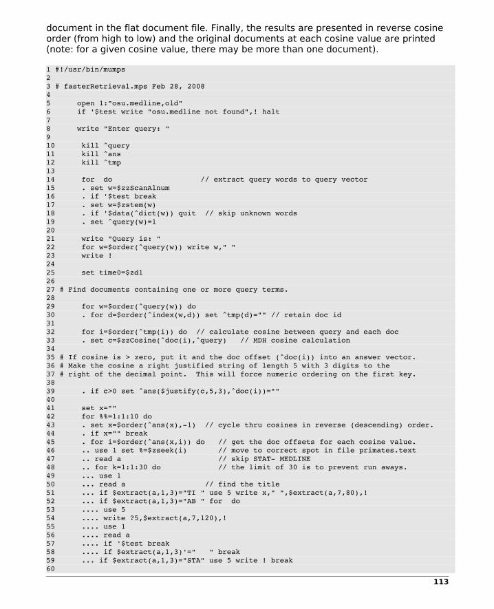
document in the flat document file. Finally, the results are presented in reverse cosine order (from high to low) and the original documents at each cosine value are printed (note: for a given cosine value, there may be more than one document).

1 #!/usr/bin/mumps2 3 # fasterRetrieval.mps Feb 28, 20084 5      open 1:"osu.medline,old"6      if '$test write "osu.medline not found",! halt7 8      write "Enter query: "9 10      kill ^query11      kill ^ans12      kill ^tmp13 14      for  do                    // extract query words to query vector15      . set w=$zzScanAlnum16      . if '$test break17      . set w=$zstem(w)18      . if '$data(^dict(w)) quit  // skip unknown words19      . set ^query(w)=120 21      write "Query is: "22      for w=$order(^query(w)) write w," "23      write !24 25      set time0=$zd126 27 # Find documents containing one or more query terms.28 29      for w=$order(^query(w)) do30      . for d=$order(^index(w,d)) set ^tmp(d)="" // retain doc id31 32      for i=$order(^tmp(i)) do  // calculate cosine between query and each doc33      . set c=$zzCosine(^doc(i),^query)   // MDH cosine calculation34 35 # If cosine is > zero, put it and the doc offset (^doc(i)) into an answer vector.36 # Make the cosine a right justified string of length 5 with 3 digits to the37 # right of the decimal point.  This will force numeric ordering on the first key.38 39      . if c>0 set ^ans($justify(c,5,3),^doc(i))=""40 41      set x=""42      for %%=1:1:10 do43      . set x=$order(^ans(x),­1)  // cycle thru cosines in reverse (descending) order.44      . if x="" break45      . for i=$order(^ans(x,i)) do   // get the doc offsets for each cosine value.46      .. use 1 set %=$zseek(i)       // move to correct spot in file primates.text47      .. read a                      // skip STAT­ MEDLINE48      .. for k=1:1:30 do             // the limit of 30 is to prevent run aways.49      ... use 150      ... read a                  // find the title51      ... if $extract(a,1,3)="TI " use 5 write x," ",$extract(a,7,80),!52      ... if $extract(a,1,3)="AB " for  do53      .... use 554      .... write ?5,$extract(a,7,120),!55      .... use 156      .... read a57      .... if '$test break58      .... if $extract(a,1,3)'="   " break59      ... if $extract(a,1,3)="STA" use 5 write ! break60 

113

61      write !,"Time used: ",$zd1­time0," seconds",!

yields the same results as above but takes less than 1 second.

Figure 82 Faster simple retrieval

14 Thesaurus construction

It is possible to find connections between terms based on their frequency of co-occurrence. Terms that co-occur frequently together are likely to be related and can indicate that the words may be synonyms or terms used to express a similar concept.

For example, a strong relationship such as between the words artificial and intelligence in a computer science data base is due to the phrase artificial intelligence which names a branch of computing. In this case, the relationship is not that of a synonym. Similarly, in the medical data base terms such as circadian rhythm and vena cava and herpes simplex are concepts expressed as more than one term.

On the other hand, as seen below, words like synergism and synergistic, cyst and cystic, schizophrenia and schizophrenic, nasal and nose, and laryngeal and larynx are examples of synonym relationships.

In other cases, the relationship is not so tight so as to be a full synonym but express a categorical relationship such as anesthetic and halothane, analgesia and morphine, nitrogen and urea, and nurse and personnel.

Regardless of the relationship, a thesaurus table can be constructed giving a list of related. With this information it is then possible to:

1. augment queries with related words to improve recall; 2. combine multiple related infrequently occurring terms into broader, more

frequently occurring categories terms; and, 3. create middle frequency composite terms from otherwise unusable high

frequency component terms.

In its simplest form, we construct a square term-term correlation matrix which gives the frequency of co-occurrence of terms with one another. Thus, if some term A occurs in 20 documents and if term B also occurs in these same documents, the term-term correlation matrix cell for row A and column B will have a value of 20. A term-term correlation matrix's lower diagonal matrix is the same as the upper diagonal matrix since the relationship between term A and B is always the same as the relationship between term B and A. The diagonal itself is the count of the number of documents in which the term occurs.

Calculating a complete term-term correlation matrix based on all documents in a large collection can be very time consuming. In most cases, a term-term matrix potentially contains many billions of elements (the square of the number of vocabulary terms) summed over the entire collection of documents. In practice, however, it is only necessary to sample a representative part of the total collection. That is, you can calculate a representative matrix by looking at every fifth, tenth or twentieth document, etc., depending on the total size of the collection.

114

As many collections can contain clusters of documents concerning specific topics, it is probably better to sample across all the documents than to only process each document in some leading fraction of the collection. Further, as many words never occur with others, especially in technical collections such as the OSU medical data base, the term-term matrix in a technical collection is likely be sparse. More general topic collections, however, will probably have matrices that are less sparse.

14.1 Basic Term-Term Co-Occurrence Matrix

The term-term co-occurrence matrix, also known as the term connection matrix, is an N x N square matrix, where N is the number of terms in the vocabulary, whose elements give the number of documents associated with each pair of terms. More formerly, it is:

TermTerm=DocTermT⋅DocTerm

That is, the product of the document term matrix DocTerm with its transpose.

In the TermTerm matrix, the rows and columns are term identifiers and the cells addressed are the number of documents which contained both terms. Here the elements of DocTerm are binary: a 0 indicates the term is not present and a 1 indicates the term is present.

Alternatively, in terms of the DocTerm matrix with elements dij, for document i and term j, the elements ttjk for terms j and k of the TermTerm matrix can be calculated as:

tt jk=d1j d 1kd 2jd 2kd 3jd 3k ....dNj dNk

Or, in other words, the similarity between term i and term j is the sum of the number of times they co-occur in a document.

For example, is you have 3 three documents entitled:

Doc1 = Pseudomonas-aeruginosa cystic-fibrosis.Doc2 = Pseudomonas-aeruginosa immune responseDoc3 = Immune complexes in cystic-fibrosis

Then the document term matrix DocTerm and its transpose DocTermT for the terms (column headings) pseudomonas-aeruginosa, immune, cystic-fibrosis, response, and complexes will be:

DocTerm=101001101001101 DocTermT=

110011101010001

Consequently, the Term-Term matrix will thus be:

115

TermTerm=DocTermT⋅DocTerm=2111012111112011101001101

In TermTerm above, each row and column correspond to a term, and the diagonal

gives the number of documents each term occurs in. Thus, the first term, pseudomonas-aeruginosa, occurs in two documents and co-occurs once with terms immune, cystic-fibrosis, and response but not with complexes. On the other hand, term complexes, the last term, occurs in one document and co-occurs once with immune and cystic-fibrosis.

A brief Mumps program to do the above is given in Figure 83. In this figure, the global array ^doc is a binary DocTerm matrix similar to the above where a 1 indicates that a term was present and a 0 indicates it was not.

1 #!/usr/bin/mumps 2 3  k ^docT,^tt 4 5  do $zzTranspose(^doc,^docT) 6 7  s k=$zzmultiply(^docT,^doc,^tt) 8 9  f i=1:1:5 w ! f j=1:1:5 w ^tt(i,j)," " 

Figure 83 Term-term matrix

The basic term-term correlation matrix calculation shown in Figure 84 initially yields a sparse matrix of term-term counts. This is also called a term connection matrix in that its elements give the number of documents that are connected to one another through a given term.

The program in Figure 84 proceeds by taking each document d in the doc-term matrix and selecting each term w in document d. For each term w, it selects those terms w1 in d which are alphabetically greater than w. For each pair of terms {w,w1}, it increments the co-occurrence count (or instantiates it with a value of 1 if it did not exist) of the cell in term-term matrix ^tt at row w and column w1. Effectively, this produces an upper diagonal matrix but no values on the diagonal itself are calculated.

The term-term matrix is then examined and those elements having a frequency of co-occurrence below a threshold are deleted (adjust this value depending on collection size). The Cosine is calculated between the term vectors and this becomes the value of the term-term matrix element. The results sorted by cosine are here:

http://www.cs.uni.edu/~okane/source/ISR/medline.tt.sorted.gz.

The results sorted by frequency of co-occurrence are here:

http://www.cs.uni.edu/~okane/source/ISR/medline.ttx.sorted.gz.

116

The complete term-term table is

http://www.cs.uni.edu/~okane/source/ISR/medline.ttw.gz

1 #!/usr/bin/mumps 2 3 # tt.mps January 18, 2011 4 5       kill ^tt 6 7       set min=$zgetenv("MINTT") 8       if min="" set min=5 9 10       for d=$order(^doc(d)) do 11       . for w=$order(^doc(d,w)) do 12       .. for w1=w:$order(^doc(d,w1)):"" do 13       ... if w1=w quit 14       ... if $data(^tt(w,w1)) set ^tt(w,w1)=^tt(w,w1)+1 15       ... else  set ^tt(w,w1)=1 16 17       for w1=$order(^tt(w1)) do 18       . for w2=$order(^tt(w1,w2)) do 19       .. if ^tt(w1,w2)<min kill ^tt(w1,w2) quit 20       .. write ^tt(w1,w2)," ",w1," ",w2,!

Figure 84 Term-Term correlation matrix

Frequency

117

Figure 85 Frequency of term co-occurrences

In Figure 85, the frequency of co-occurrence (number of times two words co-occur together) for the entire OSU collection is plotted against rank. The vertical axis represents the number of times two terms co-occur and the horizontal axis gives the rank of the term pair when sorted by this frequency of co-occurrence. That is, the term pair that co-occur the most frequently (a bit less than 1200 times) appears first (leftmost), the term pair co-occurring next most frequently next, and so on.

As can be seen, the frequency of co-occurrence drops off rapidly to a relatively constant, slowly declining value. Thus, only a few term pairs in this vocabulary, roughly the top 300, stand out as significantly more likely to co-occur than the remainder of the possible combinations due to chance alone.

The TermTerm2 matrix calculated as:

ttkm2=∑

p=1

N

∑i=1

N

∑j=1

N

d ik d pk d pmd jm

gives the second order connection matrix. For any row term k and any column term m, the value of the matrix element is the number on intermediate documents they have in common. Thus, for example, if some term A does not co-occur with term C but they both co-occur with one term B, the value of the element would be 1. Thus, there is an indirect connection between term A and term B.

TermTerm2=TermTerm⋅TermTerm=7654 2686 4 4567244 42312 4413

Thus, the values in the matrix (with rows and columns denoted as pseudomonas-

aeruginosa, immune, cystic-fibrosis, response, and complexes) for terms complexes and pseudomonas-aeruginosa (at row 1, column 5 or row 5 column 1) have values of 2 indicating that even though these terms to not co-occur together, they mutually co-occur with 2 terms (cystic-fibrosis and immune). For terms that do co-occur in the same document, the value is the number of terms in the documents themselves.

14.2 Advanced Term Term Similarity Matrix

Salton (Salton 1983) proposes the formula:

similarity Termk ,Termh=∑i=1

n

t ik t ih

∑i=1

n

t ik 2∑i=1

n

t ih2−∑i=1

n

t ik t ih

118

where t ik is the frequency of occurrence of term k in document i. The numerator is the sum of the co-occurrences of terms k and h and the denominator is the sum of the squares of the independent frequency of occurrences of the terms separately minus the frequency of co-occurrence. Basically, if two terms never co-occur the result will be zero and if they co-occur always, the result will be one. A program to calculate the term-term similarity matrix is given in Figure 86.

1 #!/usr/bin/mumps 2 3  # tt.mps January 25, 2011 4 5    kill ^tt 6 7   set min=$zgetenv("MINTT") 8   if min="" set min=5 9 10  for d=$order(^doc(d)) do 11  . for w=$order(^doc(d,w)) do 12  .. for w1=w:$order(^doc(d,w1)):"" do 13  ... if w1=w quit 14  ... if $data(^tt(w,w1)) set ^tt(w,w1)=^tt(w,w1)+1 15  ... else  set ^tt(w,w1)=1 16 17  for w1=$order(^tt(w1)) do 18  . for w2=$order(^tt(w1,w2)) do 19  .. if ^tt(w1,w2)<min kill ^tt(w1,w2) quit 20  .. set w1x=0,w2x=021  .. for d=$order(^doc(d)) do22  ... set:$data(^doc(d,w1)) w1x=^doc(d,w1)**2+w1x 23  ... set:$data(^doc(d,w2)) w2x=^doc(d,w2)**2+w2x 24  .. set ^tt(w1,w2,1)=^(tt(w1,w2)/(w1x+w2x­^tt(w1,w2)) 25  .. write ^tt(w1,w2,1)," ",^tt(w1,w2)," ",w1," ",w2,!

Figure 86 Term-term similarity matrix

Unlike the raw term-term co-occurrence count, this method takes into account underlying word usage frequency. The basic term-term co-occurrence count shown first is biased in that it favors higher frequency terms. Some lower frequency terms may have usage profiles with one another that indicate a greater similarity.

14.3 Position Specific Term-Term Matrix

Another modification to improve term-term detection, shown in Figure 87, involves retaining during document scanning the relative positions of the words with respect to one another in the collection. Then, when calculating the term-term matrix, proximity can be taken into account. If you add a new matrix to the scanning code above in addition to ^doc() named ^p(DocNbr,Word,Position) which in the third index position, retains for each word in each document the position(s) which the word occurs in relative to the beginning of the document (abstracts and titles), it becomes possible to attenuate the strength of co-occurrences by the proximity of the co-occurrence.

Subsequently, the term-term calculation becomes: for each document k, for each term i in k, for each other term j where j is alphabetically higher than i, for each position m of term i, and each position n of term j, calculate and sum weights for ^tt(i,j) based on the distance between the terms. The distance is calculated with the formula:

119

set dd=$zlog(1/$zabs(m­n)*20+1)\1 

which yields values of:

$zabs(m­n)=1 result=3 $zabs(m­n)=2 result=2 $zabs(m­n)=3 result=2 $zabs(m­n)=4 result=1 $zabs(m­n)=5 result=1 $zabs(m­n)=6 result=1 $zabs(m­n)=7 result=1 $zabs(m­n)=8 result=1 $zabs(m­n)=9 result=1 $zabs(m­n)=10 result=1 $zabs(m­n)=11 result=1 $zabs(m­n)=12 result=0 $zabs((m­n)=13 result=0 $zabs(m­n)=14 result=0 $zabs(m­n)=15 result=0 

Thus, words immediately next to one another receive a score of three while words more than eleven positions apart receive a score of zero. For each pair {i,j} a third level index is summed which is the signed difference between m and n. Eventually, a positive or negative value for this term indicates a preference for which term appears first most often. Values of zero or near zero indicate that the terms appear in no specific order relative to one another. The program then calculates a histogram giving the number of term pairs at increasing scores (see link below). For example, there were nearly 400,000 word combinations the sum of whose scores was one. Alternatively, there was one pair of words whose co-occurrence score sum, calculated as above, was 1,732 (coron and artery). The length of the histogram bars are based on the logarithm of the value displayed to the left so as to make the graph more readable.

1 #!/usr/bin/mumps2 3 # proximity.mps March 13, 20084 5       set %=$zStopInit("good") // loads stop list into a C++ container6 7       open 1:"translated.txt,old"8       if '$test write "translated not found",! halt9       use 110      set p=011      set doc=012      set M=2000013 14      for  do15      . use 116      . set word=$zzScan17      . if '$test break18      . if word="xxxxx115xxxxx" set off=$zzScan,doc=$zzScan,p=0 quit // new abstract19      . if '$zStopLookup(word) quit  // is "word" in the good list20      . set p=p+121      . set ^p(doc,word,p)=""22 23      use 524      close 1

120

25      set ^DocCount(1)=doc26 27 # ttx term­term correlation matrix28 # calculate term­term proximity coefficients within env words29 30 31      kill ^tt  //* delete any old term­term correlation matrix32 33      write !!,"Term­Term Correlation [ttx.mps] ",$zd,!34 35 #++++++++++++++++++++++++++++++++++++++++++++++++++++++++++++++++++++++36 # for each document k, sum the co­occurrences of words i and j37 #++++++++++++++++++++++++++++++++++++++++++++++++++++++++++++++++++++++38 39      Open 1:"ttx.tmp,new"40 41 # for each document k42 43      for  k=$order(^p(k)) do44 45 # for each term i in p k46 47      . for  i=$order(^p(k,i)) do48 49 # for each other term j in doc k50 51      .. set j=i52      .. for  do53      ... set j=$order(^p(k,j))54      ... if j="" break55 56 # for each position m of term i in doc k57 58      ... for  m=$order(^p(k,i,m)) do59 60 # for each position n of term j in doc k61 62      .... for  n=$order(^p(k,j,n)) do63 64 # calculate and store weight based on proximity65 66      ..... set dd=$zlog(1/$zabs(m­n)*20+1)\167      ..... if dd<1 quit68      ..... if '$Data(^tt(i,j)) set ^tt(i,j)=dd,^tt(i,j,1)=n­m69      ..... else  set ^tt(i,j)=^tt(i,j)+dd,^tt(i,j,1)=^tt(i,j,1)+(n­m)

Figure 87 Proximity Weighted Term-Term Matrix

Figure 88 contains example correlations for specific words while Figure 89 contains some of the top ranking term-term correlations. In Figure 89 the first column gives the sum of the proximity scores as calculated on line 69 in Figure 87 while last column gives net difference in the positions as calculated in lines 71 and 72 in Figure 87. Thus, the last column indicates which word tends to precede which. A large positive number favors the order shown while a large negative number favors the reverse order. A number near zero indicates that the words are likely to appear in either order.

*** apnea     sleep[254] 

*** argon     laser[240] 

*** arrest 

121

    cardiac[296] 

*** arrhythmia     ventricle[400] 

*** arterial     artery[184] coron[174] decrease[359] oxygen[328] pulmon[425] venous[315] 

*** arteries     carotid[202] cerebre[270] coron[285] 

*** artery     aneurysm[308] anterior[229] arterial[184] carotid[602] catheter[191]     cerebre[408] coron[1732] hypertension[182] infarct[192] myocardial[197]     occlusion[297] pulmon[825] renal[302] stenosis[255] vein[186] ventricle[262] 

*** arthrit     rheumatoid[779] 

*** assay     immunosorbent[231] 

*** atopic     dermatit[173] 

*** atri     fibrillate[237] ventricle[268] ...

*** diabete     mellitus[589] neuropathy[189] retinopathy[378] 

*** diagnose     biopsy[322] cancer[255] carcinoma[213] children[202] disorder[193]     evaluate[296] examination[247] lesion[239] manage[201] medical[189]     nurs[407] physician[173] procedure[174] symptom[236] 

*** dialysis     ambulatory[174] contine[219] peritoneal[439] 

*** diastolic     systolic[233] ventricle[291] 

*** diet     carbohydrate[247] casein[247] cholesterol[234] food[326] intake[562]     norm[175] weight[361] 

*** disk     intervertebre[233] 

*** disord     depressive[245] disorder[249] 

*** disorder     diagnose[193] disord[249] ment[354] 

*** distress     respiratory[270] 

*** diversion     urin[213] 

*** dogs     anesthetize[198] coron[436] myocardial[225] ventricle[270] 

122

*** doppler     echocardiography[236] 

*** dosage     radiation[192]

Figure 88 Proximity Weighted Term-Term Corellations

1721    infarct myocardial                      ­465  1445    dens lipoprotein                        73  1184    abstract word                           1184  1128    magnetic resonance                      376  1095    cord spin                               ­309  1057    lymph node                              313   964    arthrit rheumatoid                      ­307   936    female male                             ­43   878    cholesterol lipoprotein                 43   872    blind double                            ­304   859    compute tomography                      255   811    imag resonance                          ­189   762    carry out                               262   742    determine whether                       321   733    cholesterol dens                        ­137   686    mitr valve                              114   660    state unit                              ­240   649    centre nerv                             221   639    amino sequence                          ­7   638    aortic valve                            194   633    guinea pig                              32   629    care health                             ­97   625    imag magnetic                           ­439   610    cystic fibrosis                         179   587    head neck                               149   566    death sudden                            ­191   563    biopsy specimen                         230   558    electron microscopy                     111   548    marrow transplant                       113   544    tract urin                              ­156   544    diabete mellitus                        161   531    erratum publish                         ­177   530    sensit specificity                      210   530    morbid mort                             110   522    resistance vascular                     ­151   522    excretion urin                          ­283   522    ejection fraction                       130   519    cerebrospinal fluid                     106   517    coli escherichia                        ­246   513    diastolic end                           ­58   508    man old                                 ­207   500    anti monoclon                           ­97   475    state steady                            ­174   470    erythematosus lupu                      ­134   469    randomize trial                         143   466    diastolic systolic                      ­58

Figure 89 Ranked Proximity Weighted Term-Term correlations

http://www.cs.uni.edu/~okane/source/ISR/prox.gz

and

123

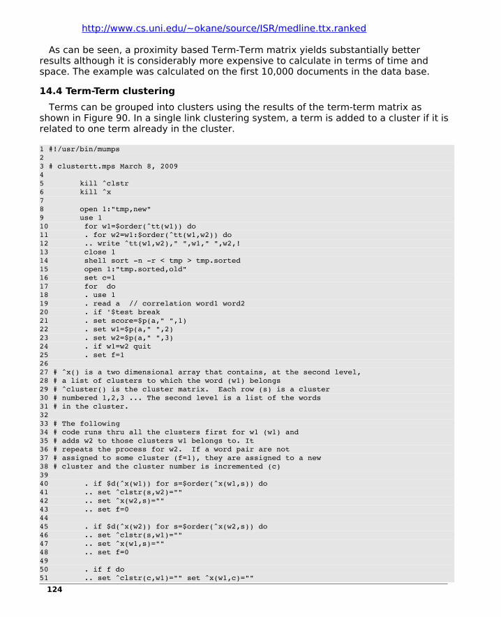
http://www.cs.uni.edu/~okane/source/ISR/medline.ttx.ranked

As can be seen, a proximity based Term-Term matrix yields substantially better results although it is considerably more expensive to calculate in terms of time and space. The example was calculated on the first 10,000 documents in the data base.

14.4 Term-Term clustering

Terms can be grouped into clusters using the results of the term-term matrix as shown in Figure 90. In a single link clustering system, a term is added to a cluster if it is related to one term already in the cluster.

1 #!/usr/bin/mumps2 3 # clustertt.mps March 8, 20094 5        kill ^clstr6        kill ^x7 8        open 1:"tmp,new"9        use 110        for w1=$order(^tt(w1)) do11        . for w2=w1:$order(^tt(w1,w2)) do12        .. write ^tt(w1,w2)," ",w1," ",w2,!13        close 114        shell sort ­n ­r < tmp > tmp.sorted15        open 1:"tmp.sorted,old"16        set c=117        for  do18        . use 119        . read a  // correlation word1 word220        . if '$test break21        . set score=$p(a," ",1)22        . set w1=$p(a," ",2)23        . set w2=$p(a," ",3)24        . if w1=w2 quit25        . set f=126 27 # ^x() is a two dimensional array that contains, at the second level,28 # a list of clusters to which the word (w1) belongs29 # ^cluster() is the cluster matrix.  Each row (s) is a cluster30 # numbered 1,2,3 ... The second level is a list of the words31 # in the cluster.32 33 # The following34 # code runs thru all the clusters first for w1 (w1) and35 # adds w2 to those clusters w1 belongs to. It36 # repeats the process for w2.  If a word pair are not37 # assigned to some cluster (f=1), they are assigned to a new38 # cluster and the cluster number is incremented (c)39 40        . if $d(^x(w1)) for s=$order(^x(w1,s)) do41        .. set ^clstr(s,w2)=""42        .. set ^x(w2,s)=""43        .. set f=044 45        . if $d(^x(w2)) for s=$order(^x(w2,s)) do46        .. set ^clstr(s,w1)=""47        .. set ^x(w1,s)=""48        .. set f=049 50        . if f do51        .. set ^clstr(c,w1)="" set ^x(w1,c)=""

124

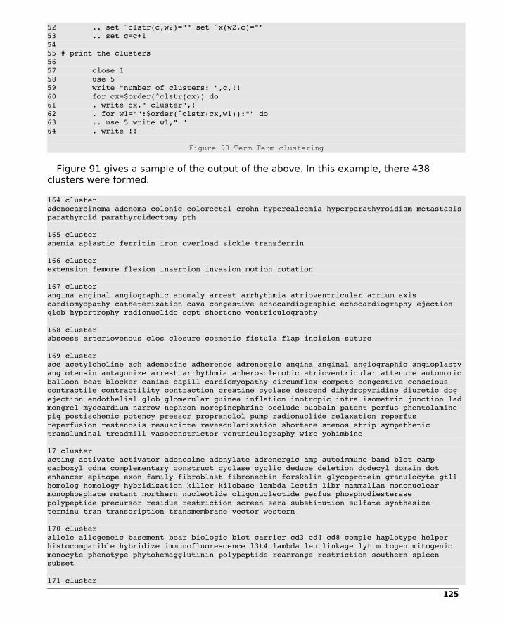
52        .. set ^clstr(c,w2)="" set ^x(w2,c)=""53        .. set c=c+154 55 # print the clusters56 57        close 158        use 559        write "number of clusters: ",c,!!60        for cx=$order(^clstr(cx)) do61        . write cx," cluster",!62        . for w1="":$order(^clstr(cx,w1)):"" do63        .. use 5 write w1," "64        . write !!

Figure 90 Term-Term clustering

Figure 91 gives a sample of the output of the above. In this example, there 438 clusters were formed.

164 clusteradenocarcinoma adenoma colonic colorectal crohn hypercalcemia hyperparathyroidism metastasis parathyroid parathyroidectomy pth 

165 clusteranemia aplastic ferritin iron overload sickle transferrin 

166 clusterextension femore flexion insertion invasion motion rotation 

167 clusterangina anginal angiographic anomaly arrest arrhythmia atrioventricular atrium axis cardiomyopathy catheterization cava congestive echocardiographic echocardiography ejection glob hypertrophy radionuclide sept shortene ventriculography 

168 clusterabscess arteriovenous clos closure cosmetic fistula flap incision suture 

169 clusterace acetylcholine ach adenosine adherence adrenergic angina anginal angiographic angioplasty angiotensin antagonize arrest arrhythmia atherosclerotic atrioventricular attenute autonomic balloon beat blocker canine capill cardiomyopathy circumflex compete congestive conscious contractile contractility contraction creatine cyclase descend dihydropyridine diuretic dog ejection endothelial glob glomerular guinea inflation inotropic intra isometric junction lad mongrel myocardium narrow nephron norepinephrine occlude ouabain patent perfus phentolamine pig postischemic potency pressor propranolol pump radionuclide relaxation reperfus reperfusion restenosis resuscitte revascularization shortene stenos strip sympathetic transluminal treadmill vasoconstrictor ventriculography wire yohimbine 

17 clusteracting activate activator adenosine adenylate adrenergic amp autoimmune band blot camp carboxyl cdna complementary construct cyclase cyclic deduce deletion dodecyl domain dot enhancer epitope exon family fibroblast fibronectin forskolin glycoprotein granulocyte gt11 homolog homology hybridization killer kilobase lambda lectin libr mammalian mononuclear monophosphate mutant northern nucleotide oligonucleotide perfus phosphodiesterase polypeptide precursor residue restriction screen sera substitution sulfate synthesize terminu tran transcription transmembrane vector western 

170 clusterallele allogeneic basement bear biologic blot carrier cd3 cd4 cd8 comple haplotype helper histocompatible hybridize immunofluorescence l3t4 lambda leu linkage lyt mitogen mitogenic monocyte phenotype phytohemagglutinin polypeptide rearrange restriction southern spleen subset 

171 cluster

125

avidin biotin glutathione paraffin peroxidase 

172 clusterarteriosus ductus occlude patent 

173 clusteractuarial adjuvant cisplatin cours distant irradiate radiotherapy squam 

174 clusteralzheimer behaviore chorionic cognitive cortex dementia gestational her home intrauterine labor memory ment mother neuropsychological perinatal pregnant retardate tangle task trimester 

175 clusterace acetylcholine ach adherence angiotensin antagonize attenute blocker compete contractile contractility contraction dihydropyridine diuretic endothelial endothelium guinea inotropic isometric junction norepinephrine pig potency propranolol relax relaxation strip yohimbine 

Figure 91 Term Clusters

The full results for a 20,000 abstract run are

http://www.cs.uni.edu/~okane/source/ISR/medline.cluster-tt

14.5 Construction of Term Phrases

Salton notes that recall can be improved if additional, related terms are added to a query. Thus, a query for antenna will result in more hits in the data base if the related term aerial is added. An increase in recall, however, is often accompanied by a decrease in precision. As is evidenced by the fact that while aerial is a commonly used synonym for antenna, as in television aerial, it can also refer to a dance move, a martial arts move, skiing, various musical groups and performances, and any activity that is done at a height (e.g., aerial photography). Thus, adding it to a query with antenna has the potential to introduce many extraneous hits.

Identification of phrases, however, has the potential to increase precision. These are composite terms of high specificity - such as television aerial noted above. While both television and aerial individually are broad terms, the phrase television aerial or television antenna is quite specific. When a phrase is identified, it becomes a single term in the document vector.

Phrases can be identified by both syntactic and statistical methods. While techniques may take into account term proximity as well as co-occurrence such as suggested above, Salton suggests the following simpler formula for construction of term phrases:

^Cohesion(i,j) = SIZE_FACTOR * (^tt(i,j)/(^dict(i)*^dict(j)))

The code to perform the cohesion calculation is shown in Figure 92.

1 #!/usr/bin/mumps2 3 # cohesion.mps March 25, 20104 5 # phrase construction6 7      open 1:"tmp,new"8 

126

9      use 110      for i=$order(^tt(i)) do11      . for  j=$o(^tt(i,j)) do12      .. set c=^tt(i,j)/(^dict(i)*^dict(j))*100000\113      .. if c>0 write c," ",i," ",j,!14 15      shell sort ­nr < tmp > cohesion.results16      shell rm tmp

Figure 92 Term Cohesion

Figure 93 gives a sample of the results.

347 prick allergen 347 philadelphia abl 347 monomorphic induc 347 lupu erythematosus 347 induc monomorphic 346 sod dismutase 346 penile erectile 346 nicardipine dihydropyridine 346 fibrinopeptide coagulate 346 cardioplegia cardioplegic 346 aldehyde isozyme 345 thromboembolism anticoagulant 345 preterm chorioamnionit 345 polymorphism informative 345 intervertebre disc 345 agglutinin galactose 345 activator plasminogen 344 superoxide scavenger 344 subaortic outflow 344 pneumocyst pneumonia

Figure 93 Term Cohesion Results

The full OSU MEDLINE results are here:

http://www.cs.uni.edu/~okane/source/ISR/medline.cohesion.sorted.gz

and the Wikipedia results are here:

http://www.cs.uni.edu/~okane/source/ISR/wiki.cohesion.sorted.gz .

Salton notes that this procedure can sometimes result in unwanted connections such as Venetian blind and blind Venetian. For that reason, the aggregate relative order of the terms, as shown above, can help to decide when two terms are seriously linked. That is, if the order is strongly in favor of on term preceding another, this indicates a probable phrase; on the other hand, if the relative order is in neither direction, this is probably not a phrase.

15 Document-Document Matrix

It is also possible to construct Document-Document Matrices giving the correlation between all documents which have significant similarities with one another as shown in Figure 94. Such a matrix can be used to generate document clusters and for purposes of document browsing by permitting the user to navigate related documents to the one

127

being viewed. That is, if a user finds on of the retrieved articles of particular interest, a Document-Document matrix can be used to quickly identify other documents related to the document of interest. The source code is shown below and the Wikipedia results are

http://www.cs.uni.edu/~okane/source/ISR/wiki.dd2.gz

and the OSU MEDLINE results are

http://www.cs.uni.edu/~okane/source/ISR/medline.dd2.gz.

The program only calculates the cosines between documents that share at least one term rather than between all possible documents.

1 #!/usr/bin/mumps 2 3 # docdoc7.mps Mar 5, 2011 4 5       write !!,"Document­document matrix ",$zd,! 6 7       set wgt=$zgetenv("WGT") 8       if wgt="" set wgt=5 9       write "Min count=",wgt,!! 10 11       kill ^dd 12 13       open 1:"dd.1,new" 14 15       use 1 16       for w=$order(^index(w)) do 17       . for d1=$order(^index(w,d1)) do 18       .. for d2=d1:$order(^index(w,d2)):"" do 19       ... write d1," ",d2,! 20 21       close 1 22 23       shell/p sort < dd.1 | uniq ­c | sort ­rn 24 25       use 6 26       for  do 27       . read a 28       . if '$test break 29       . set a=$zb(a) 30       . set c=$piece(a," ",1) 31       . if c<wgt break 32       . set d1=$piece(a," ",2) 33       . set d2=$piece(a," ",3) 34       . if d1=d2 quit 35       . set ^dd(d1,d2)=$j($zzCosine(^doc(d1),^doc(d2)),1,3) 36 37       close 6 38       open 1:"doc­doc,new" 39       use 1 40 41       for d1=$order(^dd(d1)) do 42       . if $order(^dd(d1,""))="" quit 43       . write !,d1,": ",?10 44       . for d2=$order(^dd(d1,d2)) do 45       .. write d2,"(",^dd(d1,d2),") " 46 47       use 5 48       close 1 

128

Figure 94 Doc-Doc matrix

15.1 File and Document Clustering (Salton83, pages 215-222)

(see also:

File and Document Clustering (Salton83, pages 215-222); see also:

http://www.cs.uni.edu/~okane/115/isrscans/clustering1/

Hierarchical Clustering

http://www.resample.com/xlminer/help/HClst/HClst_intro.htm

Web Document Clustering: A Feasibility Demonstration (pdf)

http://www.cs.washington.edu/homes/etzioni/papers/sigir98.pdf

Document Clustering

http://www-2.cs.cmu.edu/~lemur/3.1/cluster.html

Hierarchical Document Clustering (pdf)

h ttp://www.cs.sfu.ca/~ester/papers/Encyclopedia.pdf

A comparative study of generative methods for document clustering (pdf)

http://www.lans.ece.utexas.edu/upload/comptext.pdf

Demonstration of hierarchical document clustering (pdf)

http://www-2.cs.cmu.edu/~hdw/JCDL01_valdes.pdf

Relationship-based Clustering and Cluster Ensembles for High-dimensional Data Mining

http://www.lans.ece.utexas.edu/~strehl/diss/htdi.html

The program cluster.mps in Figure 95 uses a single link clustering technique similar to that used in the term clustering above. The program generates and then reads a file of document-document correlations sorted in reverse (highest to lowest) correlation order.

1 #!/usr/bin/mumps2 3 # cluster.mps March 9, 20084 5        kill ^clstr6        kill ^x7 8        open 1:"tmp,new"9        use 110        for d1="":$order(^dd(d1)):"" do11        . for d2=d1:$order(^dd(d1,d2)):"" do12        .. write ^dd(d1,d2)," ",d1," ",d2,!13        close 1

129

14        set %=$zsystem("sort ­n ­r < tmp > tmp.sorted")15        open 1:"tmp.sorted,old"16        set c=117        for  do18        . use 119        . read a  // correlation doc1 doc220        . if '$test break21        . set score=$p(a," ",1)22        . set seq1=$p(a," ",2)23        . set seq2=$p(a," ",3)24        . if seq1=seq2 quit25        . set f=126 27 # ^x() is a two dimensional array that contains, at the second level,28 # a list of clusters to which the document number (seq1) belongs29 # ^cluster() is the cluster matrix.  Each row (s) is a cluster30 # numbered 1,2,3 ... The second level is a list of the document31 # numbers of those documents in the cluster. The following32 # code runs thru all the clusters first for doc1 (seq1) and33 # adds seq2 (doc2) to those clusters doc1 belongs to.  It34 # repeats the process for seq2 (doc2).  If a doc pair are not35 # assigned to some cluster (f=1), they are assigned to a new36 # cluster and the cluster number is incremented (c)37 38        . if $d(^x(seq1)) for s="":$order(^x(seq1,s)):"" do39        .. set ^clstr(s,seq2)=""40        .. set ^x(seq2,s)=""41        .. set f=042 43        . if $d(^x(seq2)) for s="":$order(^x(seq2,s)):"" do44        .. set ^clstr(s,seq1)=""45        .. set ^x(seq1,s)=""46        .. set f=047 48        . if f do49        .. set ^clstr(c,seq1)="" set ^x(seq1,c)=""50        .. set ^clstr(c,seq2)="" set ^x(seq2,c)=""51        .. set c=c+152 53 # print the clusters54 55        close 156        open 1:"osu.medline,old"57        if '$test write "missing translated.txt",! halt58        use 559        write "number of clusters: ",c,!!60        for cx="":$order(^clstr(cx)):"" do61        . use 5 write cx," cluster",!62        . for seq1="":$order(^clstr(cx,seq1)):"" do63        .. use 1 set %=$zseek(^doc(seq1)) read title64        .. use 5 write $e(title,1,120),!65        . use 5 write !

Figure 95 Document clustering

Figure 96 gives a sample output from the program in Figure 95.

1212 cluster Plasminogen activators: pharmacology and therapy. Studies on the mechanism of action of oral contraceptives with regard to fibrinolytic variables. Correlations between fibrinolytic function and acute myocardial infarction. Plasminogen activator inhibitor activity and other fibrinolytic variables in patients with coronary artery disease. 

1213 cluster Colony formation of clone­sorted human hematopoietic progenitors. 

130

Target cells for granulocyte colony­stimulating factor, interleukin­3, and interleukin­5 in differentiation pathways of Proliferative responses to interleukin­3 and granulocyte colony­stimulating factor distinguish a minor subpopulation of 

1214 cluster Double­blind randomized clinical trial of self­administered podofilox solution versus vehicle in the treatment of genita A double­blind, randomized trial of 0.5% podofilox and placebo for the treatment of genital warts in women. Patient­applied podofilox for treatment of genital warts. 

1215 cluster The p67­phox cytosolic peptide of the respiratory burst oxidase from human neutrophils. Functional aspects. Neutrophil nicotinamide adenine dinucleotide phosphate oxidase assembly. Translocation of p47­phox and p67­phox requires 

1216 cluster Nutritional concerns: need for iron. Serum transferrin receptor: a quantitative measure of tissue iron deficiency. Iron metabolism under rEPO therapy in patients on maintenance hemodialysis. Iron deficiency: definition and diagnosis. Diagnosis of iron­deficiency anemia in the elderly. Clinical utility of serum tests for iron deficiency in hospitalized patients [see comments] Quantitation of ferritin iron in plasma, an explanation for non­transferrin iron. Adequacy of iron supply for erythropoiesis: in vivo observations in humans. Iron management during recombinant human erythropoietin therapy. 

1217 cluster Intramedullary locking nails for femoral shaft fractures in elderly patients. Locked nailing of comminuted and unstable fractures of the femur. Locked intramedullary nailing of femoral shaft fractures. Intramedullary locking nails in the management of femoral shaft fractures. 

1218 cluster Stage C prostatic adenocarcinoma: flow cytometric nuclear DNA ploidy analysis. Stage B prostate adenocarcinoma. Flow cytometric nuclear DNA ploidy analysis. Stage D1 prostatic adenocarcinoma: significance of nuclear DNA ploidy patterns studied by flow cytometry. 

1219 cluster Human C5a and C5a des Arg exhibit chemotactic activity for fibroblasts. A direct in vivo comparison of the inflammatory properties of human C5a and C5a des Arg in human skin. Identification of the C5a des Arg cochemotaxin. Homology with vitamin D­binding protein (group­specific component globul Analysis of the interaction of human C5a and C5a des Arg with human monocytes and neutrophils: flow cytometric and chemo 

Figure 96 Example Document Document Clustering

The results for OSU MEDLINE are here:

http://www.cs.uni.edu/~okane/source/ISR/medline.clusters.gz

and the Wikipedia results are here:

http://www.cs.uni.edu/~okane/source/ISR/wiki.clusters.gz.

A program to generate clusters of clusters is given in Figure 97.

1 #!/usr/bin/mumps 2 # hyper­cluster.mps March 25, 2008 3 4       kill ^hc 5       set c=0,k=0 6       set min=$zgetenv("HYPMIN") 7       set wgt=$zgetenv("HYPWGT") 8       if min="" set min=0.8 9       if wgt="" set wgt=1 10 # 11 #     read the level one clusters and build 12 #     centroid vectors 13 # 14       for  do 15       . read a 16       . if '$test break 17       . if a="" quit 18       . set t=$p(a," ",1) 19       . if t="cluster" do  quit 20       .. for w=$order(^hc(c,w)) set ^hc(c,w)=^hc(c,w)/k 

131

21       .. set c=c+1,k=0 22       .. quit 23       . for w=$order(^doc(t,w)) do 24       .. if $data(^hc(c,w)) set ^hc(c,w)=^hc(c,w)+^doc(t,w) 25       .. else  set ^hc(c,w)=^doc(t,w) 26       .. set k=k+1 27 28       for i=1:1:c for w=$order(^hc(i,w)) if ^hc(i,w)<wgt kill ^hc(i,w) 29 30 # 31 #     write centroid vectors 32 # 33       write !,"Centroid vectors",!! 34       for i=1:1:c do 35       . write i," " 36       . for w=$order(^hc(i,w)) write w," (",$j(^hc(i,w),3,2),") " 37       . write !! 38 39       open 1:"tmp,new" 40 41 # 42 #     calculate cluster similarities 43 # 44       write !!,"Cluster similarities:",! 45       for i=1:1:c do 46       . for j=i+1:1:c do 47       .. s x=$zzCosine(^hc(i),^hc(j)) 48       .. if x<min quit 49       .. use 5 write i," ",j," ",x,! 50       .. use 1 write x," ",i," ",j,! 51 52       use 5 53       close 1 54 55         kill ^clstr 56         kill ^x 57 58         set %=$zsystem("sort ­n ­r < tmp > tmp.sorted") 59 60         open 1:"tmp.sorted,old" 61         set c=1 62         for  do 63         . use 1 64         . read a  // correlation doc1 doc2 65         . if '$test break 66         . set score=$p(a," ",1) 67         . set seq1=$p(a," ",2) 68         . set seq2=$p(a," ",3) 69         . if seq1=seq2 quit 70         . set f=1 71 72 # ^x() is a two dimensional array that contains, at the second level, 73 # a list of clusters to which the document number (seq1) belongs 74 # ^cluster() is the cluster matrix.  Each row (s) is a cluster 75 # numbered 1,2,3 ... The second level is a list of the document 76 # numbers of those documents in the cluster. The following 77 # code runs thru all the clusters first for doc1 (seq1) and 78 # adds seq2 (doc2) to those clusters doc1 belongs to.  It 79 # repeats the process for seq2 (doc2).  If a doc pair are not 80 # assigned to some cluster (f=1), they are assigned to a new 81 # cluster and the cluster number is incremented (c) 82 83         . if $d(^x(seq1)) for s="":$order(^x(seq1,s)):"" do 84         .. set ^clstr(s,seq2)="" 85         .. set ^x(seq2,s)="" 

132

86         .. set f=0 87 88         . if $d(^x(seq2)) for s="":$order(^x(seq2,s)):"" do 89         .. set ^clstr(s,seq1)="" 90         .. set ^x(seq1,s)="" 91         .. set f=0 92 93         . if f do 94         .. set ^clstr(c,seq1)="" set ^x(seq1,c)="" 95         .. set ^clstr(c,seq2)="" set ^x(seq2,c)="" 96         .. set c=c+1 97 98 # 99 # print the clusters 100 # 101 102         close 1 103         use 5 104         write !!,"Number of clusters: ",c,!! 105         for cx=$order(^clstr(cx)) do 106         . write "cluster ",cx,! 107         . for seq1=$order(^clstr(cx,seq1)) do 108         .. write "base cluster=",seq1,! 109         .. for cz=$order(^ct(seq1,cz)) do 110         ... write seq1,?8,^title(cz),! 111         . write ! 

Figure 97 Document hyper-clusters

16 Web Page Access - Simple Keyword Based Logical Expression Server Page

The program in Figure 98 outlines the process to build an interactive web page to access the data. At this point, we assume that the data base has been processed and the appropriate global array vectors and matrices exist. The following program will access the data base:

1 #!/usr/bin/mumps2 3 # webFinder.mps March 23, 20084 5      html Content­type: text/html &!&!6      set t=$zd17 8      html <html><body bgcolor=silver>9 10      if '$data(query) set query=""11      html <center><img src=http://sidhe.cs.uni.edu/moogle.gif border=0><br>12      html <form name="f1" method="get" action="webFinder.cgi">13      html <input type="text" name="query" size=50 maxlength=128 value="&~query~">14      html &nbsp <input type="submit" value="Search">15      html </form>16      html <form name="f1" method="get" action="webFinder.cgi">17      html <input type="hidden" name="query" value="###">18      html &nbsp <input type="submit" value="I'm Feeling Sick">19      html </form></center>20      write !21 22      if query="" write "</body></html>",! halt23 24      if query="###" do25      . set w=""

133

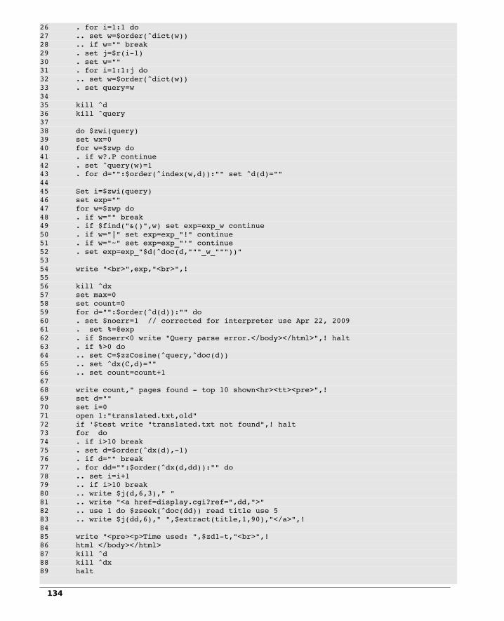
26      . for i=1:1 do27      .. set w=$order(^dict(w))28      .. if w="" break29      . set j=$r(i­1)30      . set w=""31      . for i=1:1:j do32      .. set w=$order(^dict(w))33      . set query=w34 35      kill ^d36      kill ^query37 38      do $zwi(query)39      set wx=040      for w=$zwp do41      . if w?.P continue42      . set ^query(w)=143      . for d="":$order(^index(w,d)):"" set ^d(d)=""44 45      Set i=$zwi(query)46      set exp=""47      for w=$zwp do48      . if w="" break49      . if $find("&()",w) set exp=exp_w continue50      . if w="|" set exp=exp_"!" continue51      . if w="~" set exp=exp_"'" continue52      . set exp=exp_"$d(^doc(d,"""_w_"""))"53 54      write "<br>",exp,"<br>",!55 56      kill ^dx57      set max=058      set count=059      for d="":$order(^d(d)):"" do60      . set $noerr=1  // corrected for interpreter use Apr 22, 200961      .  set %=@exp62      . if $noerr<0 write "Query parse error.</body></html>",! halt63      . if %>0 do64      .. set C=$zzCosine(^query,^doc(d))65      .. set ^dx(C,d)=""66      .. set count=count+167 68      write count," pages found ­ top 10 shown<hr><tt><pre>",!69      set d=""70      set i=071      open 1:"translated.txt,old"72      if '$test write "translated.txt not found",! halt73      for  do74      . if i>10 break75      . set d=$order(^dx(d),­1)76      . if d="" break77      . for dd="":$order(^dx(d,dd)):"" do78      .. set i=i+179      .. if i>10 break80      .. write $j(d,6,3)," "81      .. write "<a href=display.cgi?ref=",dd,">"82      .. use 1 do $zseek(^doc(dd)) read title use 583      .. write $j(dd,6)," ",$extract(title,1,90),"</a>",!84 85      write "<pre><p>Time used: ",$zd1­t,"<br>",!86      html </body></html>87      kill ^d88      kill ^dx89      halt

134

Figure 98 Browser based retrieval

In the program in Figure 98, the interpreter decodes the incoming environment variable QUERY_STRING set by the web server. It instantiates variable names with values as found in "xxx=yyy" figures contained in QUERY_STRING. In particular, this application receives a variable named "query" which is either empty, the value "###" or an optionally parenthesized logical expression involving keywords.

In the case where query is missing or empty, only the form text box is returned to the browser. In the case where the value of query is "###", a random word is selected from the vocabulary and this work becomes the value of "query"

The value of query is processed first to extract all the words provided. A global array vector named query is constructed with the words as indices. For each word, all the document numbers associated with the word in ^index() are fetched and stored in a temporary vector ^d(). When processing of all words is complete, the vector ^query() contains the words and the vector ^d() contains the document numbers of all documents that have one or more words in common with the query.

Next, the query is rescanned and a Mumps string is built. For each word in the query, a entry of the form:

$d(^doc(d,"word"))

is constructed where the value of the word is enclosed in quotes. These are connected to other similar expressions by not (~), and (&), or (!), and parentheses. Note: the input vertical bar character (|) is converted to the Mumps exclamation point "or" character (!). For example, query:

(ducks & chickens) | (rabbits & foxes) 

becomes:

($d(^doc(d,"ducks"))&$d(^doc(d,"chickens")))!($d(^doc(d,"rabbits"))&$d(^doc(d,"foxes"))) 

Note: parsing of Mumps expressions is always left to right (no precedence) unless parentheses are used.

Once the query has been re-written, the program cycles through each document number in ^d(). For each document number d, the expression built from the query is executed interpretively and the result, zero or greater than zero, determines if the document should be processed further. If the result is greater than zero, the Cosine of the document vector and the query is calculated and stored in the temporary vector ^dx(cosine,docNbr). This two part index is used so that the same Cosine value can have multiple document numbers linked to it.

Finally, the document titles (^t()) are printed in reverse cosine order. Each title is expressed as a link to the program display.cgi which will ultimately display the abstract.

The program produces output such as (OSU MEDLINE example):

135

Figure 99 Browser based retrieval

136

Unfortunately, the program above depends upon the user to be familiar with the vocabulary used in the data base. A user who spells a word incorrectly or uses a similar but different synonym is out of luck. However, there are several ways to improve data base navigation. The program above can be extended with a front end that permits point-and-click browsing for terms and term combinations. In order to do this, we used the results of the term-term matrix above with a lower threshold (thereby increasing the number of possible word combinations). The term-term matrix was used as input to a program that produced an alphabetic two level hierarchical organization of the terms that became input for a point-and-click web based display procedure.

137

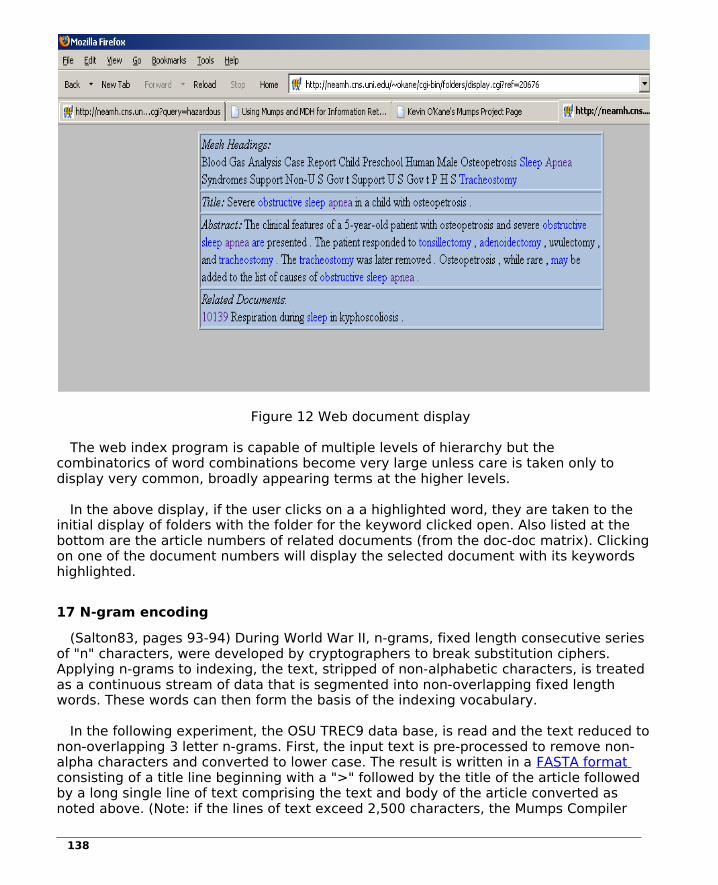
Figure 12 Web document display

The web index program is capable of multiple levels of hierarchy but the combinatorics of word combinations become very large unless care is taken only to display very common, broadly appearing terms at the higher levels.

In the above display, if the user clicks on a a highlighted word, they are taken to the initial display of folders with the folder for the keyword clicked open. Also listed at the bottom are the article numbers of related documents (from the doc-doc matrix). Clicking on one of the document numbers will display the selected document with its keywords highlighted.

17 N-gram encoding

(Salton83, pages 93-94) During World War II, n-grams, fixed length consecutive series of "n" characters, were developed by cryptographers to break substitution ciphers. Applying n-grams to indexing, the text, stripped of non-alphabetic characters, is treated as a continuous stream of data that is segmented into non-overlapping fixed length words. These words can then form the basis of the indexing vocabulary.

In the following experiment, the OSU TREC9 data base, is read and the text reduced to non-overlapping 3 letter n-grams. First, the input text is pre-processed to remove non-alpha characters and converted to lower case. The result is written in a FASTA format consisting of a title line beginning with a ">" followed by the title of the article followed by a long single line of text comprising the text and body of the article converted as noted above. (Note: if the lines of text exceed 2,500 characters, the Mumps Compiler

138

configure parameter --with-strmax=val parameter will need to be increased from its default value of 2500.)

1 # fasta.mps April 1, 20072 3      open 1:"osu.medline,old"4      if '$test write "osu.medline file not found",! halt5 6      set f=07      for  do8      . use 19      . read line10      . if '$test halt11      . if $e(line,1,2)="TI" use 5 write:f ! write "> ",$e(line,7,256),!,$$cvt(line) set 

f=1 quit12      . if $e(line,1,2)'="AB" quit13      . use 5 write $$cvt(line)14      . for  do  // for each line of the abstract15      .. use 1 read line16      .. if '$test use 5 write ! halt  // no more input17      .. if line="" break18      .. use 5 write $$cvt(line)19      . use 5 write !20      . set f=021 22      halt23 24 cvt(line)25      set buf=""26      for i=7:1:$l(line) do27      . if $e(line,i)?1A set buf=buf_$e(line,i)28      set buf=$zlower(buf)29      quit buf

Figure 100 Converting to FASTA Format in Mumps

A substantially faster version, written in C is shown in Figure 101.

1 //2 // # MDH­fasta.cpp April 1, 20073 4 #include <stdio.h>5 #include <stdlib.h>6 #include <ctype.h>7 #include <assert.h>8 #include <string.h>9 10 void cvt(char *line, char *buf) {11      int i,j;12      buf[0] = '\0';13      j = 0;14      for (i=6; line[i] != '\0'; i++)15      if (isalpha(line[i])) buf[j++] = tolower(line[i]);16      buf[j] = 0;17      }18 19 int main () {20 21      FILE *u1;22      char line[512],buf[8192];23      int i,j,f;24 25      u1 = fopen("osu.medline","r");

139

26      assert (u1 != NULL);27 28      f=0;29      while (1) {30            if (fgets(line, 512, u1) == NULL) break;31            if (strncmp(line,"TI",2) == 0) {32                  if (f) printf("\n");33                  printf("> %s",&line[6]);34                  cvt (line, buf);35                  printf("%s",buf);36                  f=1;37                  continue;38                  }39            if (strncmp(line,"AB",2) != 0)  continue;40            cvt(line,buf);41            printf("%s",buf);42            while (1) {43                  if (fgets(line, 512, u1) == NULL) break;44                  if (strlen(line) == 1) break;45                  cvt(line,buf);46                  printf("%s",buf);47                  }48            printf("\n");49            f=0;50            }51      return EXIT_SUCCESS;52 }

Figure 101 Converting to Fasta Format in C

An example of the results is shown in Figure 102 where blank lines have added between document strings for readability.

> The binding of acetaldehyde to the active site of ribonuclease: alterations in catalytic activity and effects of phosphate.thebindingofacetaldehydetotheactivesiteofribonucleasealterationsincatalyticactivityandeffectsofphosphateribonucleaseawasreactedwithccacetaldehydeandsodiumcyanoborohydrideinthepresenceorabsenceofmphosphateafterseveralhoursofincubationatdegreescphstableacetaldehydernaseadductswereformedandtheextentoftheirformationwassimilarregardlessofthepresenceofphosphatealthoughthetotalamountofcovalentbindingwascomparableintheabsenceorpresenceofphosphatethisactivesiteligandpreventedtheinhibitionofenzymaticactivityseeninitsabsencethisprotectiveactionofphosphatediminishedwithprogressiveethylationofrnaseindicatingthatthereversibleassociationofphosphatewiththeactivesitelysylresiduewasovercomebytheirreversibleprocessofreductiveethylationmodifiedrnasewasanalysedusingcprotondecouplednmrspectroscopypeaksarisingfromthecovalentbindingofenrichedacetaldehydetofreeaminogroupsintheabsenceofphosphatewereasfollowsnhterminalalphaaminogroupppmbulkethylationatepsilonaminogroupsofnonessentiallysylresiduesppmandtheepsilonaminogroupoflysineattheactivesiteppminthespectrumofrnaseethylatedinthepresenceofphosphatethepeakatppmwasabsentwhenrnasewasselectivelypremethylatedinthepresenceofphosphatetoblockallbuttheactivesitelysylresiduesandthenethylatedinitsabsencethesignalatppmwasgreatlydiminishedandthatarisingfromtheactivesitelysylresidueatppmwasenhancedtheseresultsindicatethatphosphatespecificallyprotectedtheactivesitelysinefromreactionwithacetaldehydeandthatmodificationofthislysinebyacetaldehydeadductformationresultedininhibitionofcatalyticactivity

>Reductions in breath ethanol readings in normal male volunteersfollowing mouth rinsing with water at differing temperaturesreductionsinbreathethanolreadingsinnormalmalevolunteersfollowingmouthrinsingwithwateratdifferingtemperaturesbloodethanolconcentrationsweremeasuredsequentiallyoveraperiodofhoursusingalionaedalcolmeterinhealthymalesubjectsgivenoralethanolgkgbodywtreadingsweretakenbeforeandafterrinsingthemouthwithwateratvaryingtemperaturesmouthrinsingresultedinareductioninthealcolmeterreadingsatallwatertemperaturestestedthemagnitudeofthereductionwasgreaterafterrinsingwithwateratlowertemperaturesthiseffectoccursbecauserinsingcoolsthemouthanddilutesretainedsalivathisfindingshouldbetakenintoaccountwheneverbreathanalysisisusedtoestimatebloodethanolconcentrationsinexperimentalsituations

140

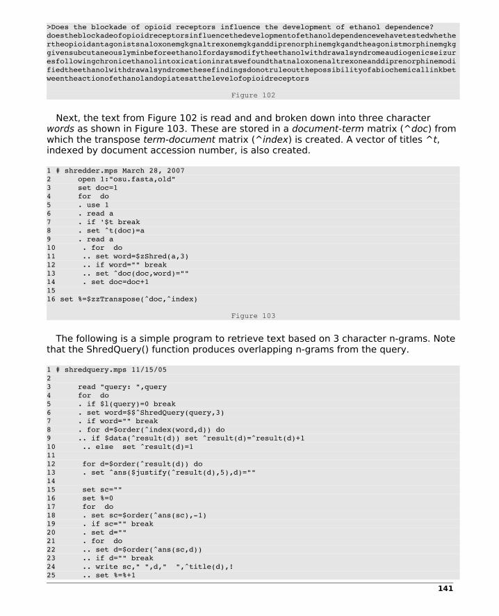
>Does the blockade of opioid receptors influence the development of ethanol dependence?doestheblockadeofopioidreceptorsinfluencethedevelopmentofethanoldependencewehavetestedwhethertheopioidantagonistsnaloxonemgkgnaltrexonemgkganddiprenorphinemgkgandtheagonistmorphinemgkggivensubcutaneouslyminbeforeethanolfordaysmodifytheethanolwithdrawalsyndromeaudiogenicseizuresfollowingchronicethanolintoxicationinratswefoundthatnaloxonenaltrexoneanddiprenorphinemodifiedtheethanolwithdrawalsyndromethesefindingsdonotruleoutthepossibilityofabiochemicallinkbetweentheactionofethanolandopiatesatthelevelofopioidreceptors

Figure 102

Next, the text from Figure 102 is read and and broken down into three character words as shown in Figure 103. These are stored in a document-term matrix (^doc) from which the transpose term-document matrix (^index) is created. A vector of titles ^t, indexed by document accession number, is also created.

1 # shredder.mps March 28, 20072      open 1:"osu.fasta,old"3      set doc=14      for  do5      . use 16      . read a7      . if '$t break8      . set ^t(doc)=a9      . read a10      . for  do11      .. set word=$zShred(a,3)12      .. if word="" break13      .. set ^doc(doc,word)=""14      . set doc=doc+115 16 set %=$zzTranspose(^doc,^index)

Figure 103

The following is a simple program to retrieve text based on 3 character n-grams. Note that the ShredQuery() function produces overlapping n-grams from the query.

1 # shredquery.mps 11/15/052 3      read "query: ",query4      for  do5      . if $l(query)=0 break6      . set word=$$^ShredQuery(query,3)7      . if word="" break8      . for d=$order(^index(word,d)) do9      .. if $data(^result(d)) set ^result(d)=^result(d)+110      .. else  set ^result(d)=111 12      for d=$order(^result(d)) do13      . set ^ans($justify(^result(d),5),d)=""14 15      set sc=""16      set %=017      for  do18      . set sc=$order(^ans(sc),­1)19      . if sc="" break20      . set d=""21      . for  do22      .. set d=$order(^ans(sc,d))23      .. if d="" break24      .. write sc," ",d,"  ",^title(d),!25      .. set %=%+1

141

26      .. if %>20 halt

Figure 104

The program from Figure 104 produces output shown in Figure 105 (some longer titles truncated and additional blanks added for readability).

sidhe:/r0/MEDLINE­TMP # shredquery.cgi

query: alcohol

10 100214  > Lithium treatment of depressed and nondepressed alcoholics 

10 100502  > Alcohol effects on luteinizing hormone releasing hormone­stimulated anterior pituitary and gonadal hormones in women.

10 100656  > Is alcohol consumption related to breast cancer? Results from the Framingham Heart Study.

10 101146  > Hyaluronic acid and type III procollagen peptide in jejunal perfusion fluid as markers of connective tissue turnover.

10 101401  > Prevalence, detection, and treatment of alcoholism in hospitalized patients 

10 10210   > Alcoholic intemperance, coronary heart disease and mortality in middle­aged Swedish men.

10 102107  > Functional and structural changes in parotid glands of alcoholic cirrhotic patients.

10 103730  > Alcohol consumption and mortality in aging or aged Finnish men [published erratum appears in J Clin Epidemiol 1989;42(7):701]

10 103762  > The role of liquid diet formulation in the postnatal ethanol exposure of rats via mother's milk.

10 103913  > Comparative effectiveness and costs of inpatient and outpatient detoxification of patients with mild­to­moderate alcohol withdrawal 

10 103926  > The effects of alcoholism on skeletal and cardiac muscle [see comments]

10 10407   > Genetic models of alcohol dependence.

10 10411   > Genetic control of liver alcohol dehydrogenase expression in inbred mice.

10 104287  > The generation of acetonemia/acetonuria following ingestion of a subtoxic dose of isopropyl alcohol.

10 10439   > Increased alcohol intake induced by chronic stimulants: is "orality" involved?

10 10440   > Naloxone attenuation of voluntary alcohol consumption.

10 10441   > Neonatal antidepressant administration suppresses concurrent active (REM) sleep and increases adult alcohol consumption in rats.

10 10444   > Is carbohydrate metabolism genetically related to alcohol drinking?

10 10449   > The antisocial and the nonantisocial male alcoholic­­II.

10 10450   > Alcohol and ambience: social and environmental determinants of intake and mood.

10 10454   > Life events in the biography of French male and female alcoholics.

Figure 105

142

The n-gram example generates very large indexing files due to the large number of fragments extracted for each abstract. To be more effective, the distribution of the fragments using an algorithm such as the Inverse Document Frequency method should be used to rank fragments for their likely usefulness in resolving articles. In practice, as is the case when dealing with actual natural language text words, fragments whose distributions are very wide and very narrow can be deleted from the indexing set. (See the section below on application of IDF to genomic data.)

143

18 Indexing Text Features in Genomic Repositories

Since the widespread adoption of the Internet in the early 1990's, there has been explosive growth in machine readable data bases both in the form of online data bases as well as web page based content. Readily accessible indexable content now easily ranges into terabytes. When indexing very large data sets, special procedures should be used to maximize efficiency. The following is a case study based on indexing the text content of genomic data bases.

Since 1990, the massive growth in genetic and protein databases has created a pressing need for tools to manage, retrieve and analyze the information contained in these libraries. Traditional tools to organize, classify and extract information have often proved inadequate when confronted with the overwhelming size and density of information which includes not only sequence and structural data, but also text that describes the data's origin, location, species, tissue sample, journal articles, and so forth. As of this writing, the NCBI (National Center for Biotechnology Information, part of the National Institutes of Health) GenBank library alone consists of nearly 84 billion bytes of data and it is only one of several data banks storing similar information. The scope and size of these databases continues to rapidly grow and will continue to do so for many years to come as will the demand for access.

A typical entry in GenBank looks like: (from: ftp://ftp.ncbi.nih.gov/genbank/ )

LOCUS AAB2MCG2 1276 bp DNA linear PRI 23-AUG-2002DEFINITION Aotus azarai beta-2-microglobulin precursor exons 2, 3, and complete cds.ACCESSION AF032093 AF032094VERSION AF032093.1 GI:3287308KEYWORDS .SEGMENT 2 of 2SOURCE Aotus azarai (Azara's night monkey) ORGANISM Aotus azarai Eukaryota; Metazoa; Chordata; Craniata; Vertebrata; Euteleostomi; Mammalia; Eutheria; Primates; Platyrrhini; Cebidae; Aotinae; Aotus.REFERENCE 1 (bases 1 to 1276) AUTHORS Canavez,F.C., Ladasky,J.J., Muniz,J.A., Seuanez,H.N., Parham,P. and

Cavanez,C. TITLE beta2-Microglobulin in neotropical primates (Platyrrhini) JOURNAL Immunogenetics 48 (2), 133-140 (1998) MEDLINE 98298008 PUBMED 9634477REFERENCE 2 (bases 1 to 1276) AUTHORS Canavez,F.C., Ladasky,J.J., Seuanez,H.N. and Parham,P. TITLE Direct Submission JOURNAL Submitted (31-OCT-1997) Structural Biology, Stanford University, Fairchild Building Campus West Dr. Room D-100, Stanford, CA 94305-5126, USACOMMENT On or before Jul 2, 1998 this sequence version replaced gi:3265029,

gi:3265028.FEATURES Location/Qualifiers source 1..1276 /organism="Aotus azarai" /mol_type="genomic DNA" /db_xref="taxon:30591" mRNA join(AF032092.1:<134..200,66..344,1023..>1050) /product="beta-2-microglobulin precursor"

144

CDS join(AF032092.1:134..200,66..344,1023..1036) /codon_start=1 /product="beta-2-microglobulin precursor" /protein_id="AAC52107.1" /db_xref="GI:3289965" /translation="MARFVVVALLVLLSLSGLEAIQRXPKIQVYSRHPAENGKPNFLN CYVSGFHPSDIEVDLLKNGKKIEKVEHSDLSFSKDWSFYLLYYTEFTPNEKDEYACRV SHVTLSTPKTVKWDRNM" mat_peptide join(AF032092.1:194..200,66..344,1023..1033) /product="beta-2-microglobulin" intron <1..65 /number=1 variation 3 /note="allele 1" /replace="g" exon 66..344 /number=2 intron 345..1022 /number=2 exon 1023..1050 /number=3 intron 1051..>1276 /number=3ORIGIN 1 caagttatcc gtaattgaaa taccctggta attaatattc atttgtcttt tcctgatttt 61 ttcaggtrct ccaaagattc aggtttactc acgtcatccg gcagagaatg gaaagccaaa 121 ttttctgaat tgctatgtgt ctgggtttca tccgtccgac attgaagttg acttactgaa 181 gaatggaaag aaaattgaaa aagtggagca ttcagacttg tctttcagca aggactggtc 241 tttctatctc ttgtactaca ccgagtttac ccccaatgaa aaagatgagt atgcctgccg 301 tgtgagccat gtgactttat caacacccaa gacagtaaag tggggtaagt cttacgttct 361 tttgtaggct gctgaaagtt gtgtatgggt agtcatgtca taaagctgct ttgatataaa 421 aaaaattcgt ctatggccat actgccctga atgagtccca tcccgtctga taaaaaaaaa 481 tcttcatatt gggattgtca gggaatgtgc ttaaagatca gattagagac aacggctgag 541 agagcgctgc acagcattct tctgaaccag cagtttccct gcagctgagc agggagcagc 601 agcagcagtt gcacaaatac atatgcactc ctaacacttc ttacctactg acttcctcag 661 ctttcgtggc agctttaggt atatttagca ctaatgaaca tcaggaaggt ataggccttt 721 ctttgtaaat ccttctatcc tagcatccta taatcctgga ctcctccagt actctctggc 781 tggattggta tctgaggcta gtaggtgggg cttgttcctg ctgggtagct ccaaacaagg 841 tattcatgga taggaacagc agcctatttt gccagcctta tttcttaata gttttagaaa 901 tctgttagta cgtggtgttt tttgttttgt tttgttttaa cacagtgtaa acaaaaagta 961 catgtatttt aaaagtaaaa cttaatgtct tcctttttct ttctccactg tctttttcat 1021 agatcgaaac atgtaaccag catcatggag gtaagttctt gaccttaatt aaatgttttt 1081 tgtttcactg gggactattt atagacagcc ctaacatgat aaccctcact atgtggagaa 1141 cattgacaga gtagcatttt agcaggcaaa gaggaatcct atagggttac attccctttt 1201 cctgtggagt ggcatgaaaa aggtatgtgg ccccagctgt ggccacatta ctgactctac 1261 agggagggca aaggaa

Figure 106

An annotated example GenBank record is available here while a complete description of the NCBI data base can be found here.

Currently, retrieval of genomic data is mainly based on well-established programs such as FASTA (Pearson, 2000, see: ) and BLAST (Altschul, 1997), that match candidate nucleotide sequences against massive libraries of sequence acquisitions. There have been few efforts to provide access to genomic data keyed to the extensive text annotations commonly found in these data sets. Among the few systems that deal with keyword based searching are the proprietary SRS system (Thure and Argos, 1993a, 1993b) and PIR (Protein Information Resource) (Wu 2003). These are limited, controlled vocabulary systems whose keys are from manually prepared annotations. To date, there have been no systems reported to directly generate indices from the genomic data sets

145

themselves. The reasons for this are several: the very large size of the underlying data sets, the size of intermediate indexing files, the complexity of the data, and the time required to perform the indexing.

The system described here, MARBL (Mumps Analysis and Retrieval from Bioinformatics Libraries), is an application to integrate multiple, very large, genomic, databases into a unified data repository through open-source components; and to provide fast, web-based keyword based access to the contents.

Sequences retrieved by MARBL can be post-processed by FASTA (Pearson, 2000), Smith-Waterman (Smith, 1981) and elements of EMBOSS (the European Molecular Biology Open Software Suite). While FASTA and, especially, Smith-Waterman, are more sensitive (Shpaer et al. 1996) than BLAST, they are also more time consuming. However, by first extracting from the larger database a subset of candidate accessions, the number of sequences to be aligned by these algorithms can be reduced significantly with corresponding reduction in the overall processing time.

18.1 Implementation

Most genomic databases include, in addition to nucleotide and protein sequences, a wealth of text information in the form of descriptions, keywords, annotations, hyper-links to text articles, journals and so forth. In many cases, the text attachments to the data are greater in size that the actual sequence data. Identifying the important keyword terms from this data and assigning a relative weight to these terms is one of the problems addressed in this system.

While indexing can be approached from the perspective of assignment to pre-existing categories and hierarchies such as the National Library of Medicine MeSH (Medical Subject Headings) (Hazel, 1997), derivative indexing is better able to adapt to changes in a rapidly evolving discipline as the terms are dynamically extracted directly from the source material rather than waiting for manual analysis. Existing keyword based genomic retrieval systems are primarily based on assignment indexing whereas the approach taken here is based on derivative indexing, where both queries and documents are encoded into a common intermediate representation and metrics are developed to calculate the coefficients of similarity between queries and documents. Documents are ranked according to their computed similarity to the query and presented to the user in rank order. Several systems employing this and related models have been implemented such as Smart (Salton, 1968, 1971, 1983, 1988), Instruct (Wade, 1988), Cansearch (Pollitt, 1987) and Plexus (Vickery, 1987a, 1987b). More recently, these approaches have been used to index Internet web pages and provide collaborative filtered recommendations regarding similar texts to book buyers at Amazon.com (Linden, 2003).

In this system, genomic accessions are represented by vectors that reflect accession content through descriptors derived from the source text by analysis of word usage (Salton,1968, 1971, 1983, 1988; Willett, 1985; Crouch, 1988). This approach can be further enhanced by identifying clusters of similar documents (El-Hamdouchi et al.,1988, 1989). Similarly, term-term co-occurrence matrices can be constructed to identify similar or related terms and these can be automatically included into queries to enhance recall or to identify term clusters. Other techniques based on terms and queries have also been explored (Salton, 1988; Williams, 1983).

146

The vector model is rooted in the construction of document vectors consisting of the weights of each term in each document. Taken collectively, the document vectors constitute a document-term matrix whose rows are document vectors. A document-term matrix can have millions of rows, more than 22 million in GenBank case, and thousands of columns (terms), more than 500,000 in GenBank. This yields a matrix with potentially trillions of possible elements which must be quickly addressable not by numeric indices but by text keys. Additionally, to enhance information retrieval speed, an inverted matrix of the same size is needed which doubles the overall storage requirements. Fortunately, however, both matrices are very sparse.

Given the nature of the problem, namely, manipulating massive, character string indexed sparse matrices, we implemented the system in Mumps.

Using Mumps global arrays, an accession-term matrix appears in the Mumps language as an array of the form: ^D(Accession,Term) where both Accession and Term are text strings. The matrix is indexed row-wise by accession codes and column-wise by text derived terms. This approach vastly simplifies implementation of the basic information storage and retrieval model. For example, the main Mumps indexing program used in the basic protocol described below is about 76 lines of code (excluding in-line C functions). The highly concise nature of the Mumps language permits rapid deployment and minimizes maintenance problems that would be the case with more complex coding systems.

FASTA (Pearson, 2000) and Smith-Waterman (Smith and Waterman, 1981) are sequence alignment procedures to match candidate protein or NA sequences to entries in a database. Sequences retrieved as a result of text searches with the system described here can be post-processed by FASTA and the Smith-Waterman. Of these, the Smith-Waterman algorithm is especially sensitive and accurate but also relatively time consuming. Using this system to isolate candidate sequences by text keywords and subsequently processing the resulting subset of the larger database, results in considerable time savings. In our experiments we used the Smith-Waterman program available as part of the FASTA package developed by W. R. Pearson (Pearson 2000). Additionally, the output of this system is compatible with the many genomic analysis programs found in the open source EMBOSS collection.

The system software is compatible with several genomic database input formats, subject to preprocessing by filters. In the example presented here, the NCBI GenBank collection was used. GenBank consists of accessions which contain sequence and related data collected by researchers throughout the world.

Two protocols were developed to index the GenBank data sets. Initially, we tried a direct, single step, vector space model protocol that constructed the accession-term matrix directly from the GenBank files. However, experiments revealed that this approach was unacceptably slow when used with large data sets. This resulted in the development of a multi-step protocol that performed the same basic functions but as a series of steps designed to improve overall processing speed. The discussion below centers on the multi-step protocol although timing results are given for both models. The work was performed on a Linux based, dual processor hyper-threaded Pentium Xeon 2.20 GHz system with 1 GB of main memory and dual 120 GB EIDE 7,200 rpm disk drives.

147

The entire GenBank data collection consisted of approximately 83.5 GB of data at the time of these experiments. When working with data sets of smaller size, relatively straightforward approaches to text processing can be used with confidence. However, when working with data sets of very large dimensions, it soon became apparent that special strategies would be needed in order to reduce the complexity of the processing problem. During indexing, as the B-tree grew, delays due to I/O became significant when the size of the data set exceeded the amount of physical memory available. At that point, the memory I/O cache became inadequate to service I/O requests without significant actual movement of data to and from external media. When this happened, CPU utilization was observed to drop to very low values while input/output activity grew to system maximum. Once page thrashing began, overall progress to index the data set slowed dramatically.

In order to avoid this problem, the multi-step protocol was devised in which the indexing tasks were divided into multiple steps and sort routines were employed in order to prepare intermediate data files so that at each stage where the database was being loaded into the B-tree, the keys were presented to the system in ascending key order thus inducing an effectively sequential data set build and eliminating page thrashing. While this process produced a significant number of large intermediate files, it was substantially faster than unordered key insertion.

18.2 Data Sets

The main data sets used were from the NCBI GenBank collection (ftp://ftp.ncbi.nlm.nih.gov)

The GenBank short directory, gbsdr.txt consisting of locus codes which, at this writing, is approximately 1.45 billion bytes in length and has approximately 18.2 million entries.

The nucleotide data, the accessions, are stored in over 300 gzip compressed files. Each file is about 220 megabytes long and consists of nucleotide accessions. We pre-process each file with a filter program that extracts text and other information. Pre-processing results in a format similar to the EMBL (European Micro Biology Laboratory) format and this makes for faster processing in subsequent steps as well as greatly reducing disk storage requirements. For example, the file gbbct1.seq, currently 250,009,587 bytes in length, reduced to 8,368,295 bytes after pre-processing.

Optionally, a list of NCBI manually derived multi-word keys from the file gbkey.idx (502,549,211 bytes). Processing of these keys is similar to that of derived keys but only a default, minimum weight is produced.

In addition to text found in the accessions, GenBank, as well as many other data resources, contains links to on-line libraries of journal articles, books, abstract and so forth. These links provided additional sources of text keys related to the accessions in the originating database.

18.3 Multiple Step Protocol

The multiple step protocol, shown in Figure 1, separated the work into several steps and was based on the observation that using system sort facilities to preprocess data files resulted in much faster database creation since the keys can be loaded into the B-tree database in ascending key order. This observation was founded in an early experiment in which an accession-term matrix was constructed by loading the keys from

148

a 5 million accessions file sorted by ascending accession key. The load procedure itself used a total of 1,032 seconds (17.2 minutes). On the other hand, loading the keys directly from a file not sorted by accession was 7.1 times slower requiring 7,333 seconds (122.2 minutes) to load.

Figure 107 Indexing GENBANK

The main text analysis procedure reads the filtered version of the accession files. Lines of text were scanned, punctuation and extraneous characters were removed, words matching entries in the stop list were discarded, and, finally, words were processed to remove suffixes and consolidated into groups based on word stems (readerb.cgi). Each term was written to an output file (words.out) along with its accession code and a code indicating the source of the data. A second file was also produced that associated each processed stem along with the original form of the term (xwords.out). The output files were sorted concurrently. The xwords.out file was sorted by term with duplicate entries discarded while the words.out file was sorted to two

149

output files: words.sorted, ordered by term then accession code, and words.sorted.2 ordered by accession code then term.

The file words.sorted was processed to count word usage (readerd.cgi). As the file was ordered by term then accession code, multiple occurrences of a word in a document appear on successive lines. The program deleted words whose overall frequency of occurrence was too low or high. Files df.lst and dict.lst were produced which contain, respectively, for each term, the number of accessions in which it appears in, and the total number of occurrences.

The file words.sorted.2 (sorted by accession code and term) was processed by readerg.cgi to produce words.counted.2 which generated for each accession, the number of times each term occurred in an accession and a string of code letters giving the original sources of the term (from the original input line codes). This file was ordered by accession and term.

The files xwords.sorted, df.lst, dict.lst and words.counted.2 were processed by readerc.cgi to produce internal data vectors and an output file named weighted.words which contained the accession code, term, the calculated inverse document frequency weight of the term, and source code(s) for the term. If the calculated weight of a term in an accession was below a threshold, it was discarded. Since the input file words.counted.2 was ordered by accession then by term, the output file weighted.words was also ordered by accession then term.

Finally, the Nrml3a.cgi constructed the term-accession matrix (^I) from the term sorted file weighted.words and Nrml3.cgi built the accession-term matrix (^D) from wgted.words.sorted which was ordered by accession and term. In this final step, the database assumed its full size and it was this step that is most critical in terms of time. As each of the matrices were ordered according to their first, then second indices, the B-tree was built in ascending key order.

18.4 Retrieval

Retrieval is via a web page interface or an interactive keyboard based program. Queries are expressed as logical expressions of terms, possibly including wildcards. Queries may be restricted to data particular sources (title, locus, etc.) or specific divisions (ROD, PRI, etc). When a query is submitted to the system it is first expanded to include related terms for any wildcards. The expression is converted into a Mumps expression and candidate accession codes of those accessions containing terms from the query are identified. The Mumps expression is applied to each identified candidate accession. A similarity coefficient between the accession and the query is calculated based on the weight of the terms in the accessions using a simple similarity formula.

From the accessions retrieved, the user can view the original NCBI accession page, save the accession list for further reference or convert the accessions to FASTA format and match the accessions against a candidate sequence with the FASTA or the Smith-Waterman algorithm. By means of the GI code from the VERSION field in the original GenBank accession, a user can access full data concerning the retrieved accession directly from NCBI. Also stored is the MEDLINE access code which provides direct entry into the MEDLINE database for the accession.

150

Retrieval times are proportional to the amount of material retrieved, the complexity of the query, and the number of accessions in which each query term appears.. For specific queries that retrieve only a few accessions, processing times less than 1 second are typical.

18.5 Results and Discussion

Some overall processing statistics for the two protocols are given in Table 1. As can be seen, the multi-step protocol performed significantly better than the basic protocol.

Table 1 - Processing Time Statistics (in minutes)

Accessions Processed 1,000,000 5,000,000 22,318,882

Multi-Step Protocol 63.9 350.8 2,016.1

Basic Protocol 246.9 1,735.61 6994.7

Figure 108

The dimensions of the final matrices are potentially of vast size: 22.3 million by 501,614 in this case. Potentially, this implies a matrix of 11.5 trillion elements. However, the matrix is very sparse and the file system stores only those elements which actually exist. After processing the entire GenBank, the actual database was only 23 GB although at its largest, before compaction of unused space, it reached 44 GB.

Evaluation of information retrieval effectiveness from a data set of this size is clearly difficult as there are few benchmarks against which to compare the results. However, NCBI distributes a file of keyword phrases with GenBank gbkey.idx (502,549,211 bytes). This file contains submission author assigned keyword phrases and associated accession identifiers. Of the 48,023 unique keys in gbkey.idx (after removal of special characters and words less than three characters in length), 26,814 keys were the same as the keys selected by MARBL. The 21,209 keys that differed were, for the most part, words of very high or low frequency that the system rejected due to preset thresholds. Alternatively, the MARBL system identified and retained a highly specific 501,614 terms, many of which were specific codes used to identify genes.

When comparing the accessions linked to keywords in gbkey.idx with MARBL derived accessions, it was clear that MARBL discovered vastly more linkages than the NCBI file identified. For example, the keyword zyxin (the last entry in gbkey.idx) was linked to 4 accessions by gbkey.idx but MARBL detected 336 accessions. In twelve other queries based on terms randomly selected from gbkey.idx, MARBL found more accessions than were listed in gbkey.idx in nine cases and the same number in three cases. On average, each MARBL derived keyword points to 130.34 accessions whereas gbkey.idx keys, on average, points to 6.80 accessions.

We compared MARBL with BLAST by entering the nucleotide sequence of a Bacillus anthracis bacteriophage that was of interest to a local researcher. BLAST retrieved 24 accessions, with one scoring 1,356, versus the next highest with a score of 50. The highest scoring accession was the correct answer, while the remainder were noise. When we entered the phrase anthracis & bacteriophage to the MARBL information

151

retrieval package, only one accession was retrieved, the same one that received the highest score from BLAST. BLAST took 29 seconds, MARBL information retrieval took 10 seconds. It should be noted, however, that BLAST searches are not based on keywords but on genomic sequences.

Mumps is an excellent text indexing implementation language (O'Kane, 1992). Mumps programs are concise and are easily maintained and modified. The string indexed global arrays, underpinned by the effectively unlimited file sizes supported by the BDB, make it possible to design very large, efficient systems with minimal effort. In all, there were 10 main indexing routines with a total of 930 lines of Mumps code (including comments) for an average of 93 lines of code per module. On the other hand, the C programs generated by the Mumps compiler amounted to 21,146 lines of code, not counting many thousands of lines in run-time support and database routines. The size of the C routines is comparable to reported code sizes for other information storage and retrieval projects such as Wade (1988) who reports that Instruct as approximately 6,000 lines of Pascal code, and Plexus (Vickery and Brooks, 1987a) reported as approximately 10,000 lines although, due to differences in features, these figures should not be used for direct comparisons.

An example of this system in its current state can be seen here.

152

19 Overview of Other Methods

19.1 Using Sort Based Techniques

19.2 Latent Semantic Model

Essentially and term-term co-occurrence method used to augment queries. An execellent example of a very bad patent award (1988) - the underlying techniques have been around since the 1960's.

References to Papers on LSI Wikipedia Entry on LSI

19.3 Single Term Based Indexing

Reference: Salton 1983.

Summary:

Single term methods view the collection as a set of individual terms. Methodologies based on this approach seek to identify which terms are most

indicative of content and to quantify the relative resolving power of each term. Documents are generally viewed as vectors of terms weighted by the product of a

term's frequency of occurrence in the document and its weight in the collection as a whole.

The vector space of a document collection may be treated as an hyperspace and the effect of a term on the space density may be taken as indicative of the term's resolving or discriminating power.

Documents may be clustered based on the similarities of their vector representations. Hierarchies of clusters may be generated.

Queries are treated as weighted vectors and the calculated similarity between a query vector and document vectors determines the ranking of a document in the results presented.

Answers to queries are ranked by recall and precision - measures of the degree of effectiveness of the methodology to find all documents in a collection relevant to a query and the degree to which irrelevant documents are included with relevant documents.

Queries may be enhanced by including terms whose usage patterns are similar to words in the original query.

19.4 Phrase Based Indexing

These are based on multiple words taken as phrases that are likely to convey greater context so as to improve precision.

153

Methods can involve thesauruses which group multiple words together into concept classes.

Methods can seek the identification of key phrases in a document. or construction of phrases from document context.

19.5 N-Gram Based Indexing

N-grams Example Code

The following link is to a collection of Mumps code that performs the operations listed above: http://www.cs.uni.edu/~okane/source/ISR/ISR115Code.tgz .

154

20 Visualization

An increasingly important aspect of IS&R is the ability to present the results to the user in a meaningful manner and interact with the user to refine his or her requests. In the early Salton experiments, queries and results were in text format only and generally entered, processed, and returned in batches. Since the widespread availability of the Internet as well and the general availability of graphical user interfaces, newer methods of rendering results can be explored. The following links give examples of several of these:

Modern Information Retrieval Chapter 10: User Interfaces and Visualization - by Marti Hearst

Visualizing the Non-Visual: spatial Analysis and Interaction with Information from Text Documents J.A. Wise, J.J. Thomas, K. Pennock, D. Lantrip, M. Pottier, A. Schur, and V. Crow (PDF file)

Visualizing the Non-Visual: Spatial Analysis and Interaction with Information from Text Documents J.A. Wise, J.J. Thomas, K. Pennock, D. Lantrip, M. Pottier, A. Schur, and V. Crow (PowerPoint File)

Internet browsing and searching: User evaluations of category map and Concept Space (PDF)

Exploring the World Wide Web with Self-Organizing Map HIBROWSE interfaces Scatter/Gather clustering

Text Searching Open Directory Open Directory Project Text Searching in Genomic Data Bases Entrez/PubMed SRS

155

21 Applications to Genomic Data Bases

In the past 15 years, genomics data bases have grown rapidly. These include both text and genetic information and the need to search them is central to research in areas such as genetic, drug discovery and medicine, to name a few.

Genetic data bases include both natural language text as well as sequences of genetic information. Data bases containing genetic data bases are primarily divided into two types: those containing protein information and those containing DNA sequences. DNA sequence data bases usually consist of natural language text together with DNA sequence information over the nucleotide alphabet of bases {ACGT}. These letters stand for:

Adenine Cytosine Guanine Thymine

DNA itself is a double stranded helix with the nucleotides constituting the links across the strands (see: here)

Protein sequence data bases are over the alphabet {ACDEFGHIKLMNPQRSTVWY} of amino acids. Sections of DNA are codes that are used to construct proteins. The order of the amino acids in a protein determine its shape, chemical activity and function.

DNA substrings become proteins through a process of translation and transcription. The DNA is divided into three letter codons which select amino acids for incorporation into the protein being built.

Over evolutionary time, DNA and resulting protein structures mutate. Thus, when searching either a protein or nucleotide data base, exact matches are not always the case. However, it has been observed that certain mutations are favored in nature while others are not. Generally speaking, this is because some mutations do not effect the functionality of the resulting proteins while other render the protein unusable.

Many searching algorithms take evolutionary mutation into account through the use of substitution matrices. These give a score as to the probability of a given substitution of one amino acid for another based on observation in nature. The BLAST substitution matrices are typical. Different matrices are used to account for the amount of presumed evolutionary distance.

21.1 GenBank

"GenBank is a component of a tri-partite, international collaboration of sequence databases in the U.S., Europe, and Japan. The collaborating database in Europe is the European Molecular Biology Laboratory (EMBL) at Hinxton Hall, UK, and in Japan, the DNA Database of Japan (DDBJ) in Mishima, Japan. Patent sequences are incorporated through arrangements with the U.S. Patent and Trademark Office, and via the collaborating international databases from other international patent offices. The database is converted to various output formats including the Flat File and Abstract Syntax Notation 1 (ASN.1) versions. The ASN.1 form of the data is included in www-

156

Entrez and network-Entrez and is also available, as is the flat file, by anonymous FTP to 'ftp.ncbi.nih.gov'." (ftp://ftp.ncbi.nih.gov/genbank/README.genbank)

Main GenBank FTP Site General Release Notes Feature Table Definitions Annotated Sample Record

EMBL/EBI (European Molecular Biology Laboratory/European Bioinformatics Institute "The European Bioinformatics Institute (EBI) is a non-profit academic organisation that

forms part of the European Molecular Biology Laboratory (EMBL). The EBI is a centre for research and services in bioinformatics. The Institute manages databases of biological data including nucleic acid, protein sequences and macromolecular structures. The mission of the EBI is to ensure that the growing body of information from molecular biology and genome research is placed in the public domain and is accessible freely to all facets of the scientific community in ways that promote scientific progress." (from: http://www.ebi.ac.uk/Information/ )

EBI Home Page EBI FTP Server

21.2 Alignment Algorithms

In bioinformatics, a researcher identifies a protein or nucleotide sequence and wants to locate similar sequences in the data base. Some of the earliest methods used involve sequence alignment. Most direct sequence alignment techniques are very compute intensive and impractical to be applied with very large data bases. However, they represent the "gold standard" for sequence matching. The following is an historical overview of alignment algorithms and their evolution.

Elementary Sequence Alignment Dot Plots Needleman-Wunch Global Alignment Smith-Waterman Local Alignment Outline of WN, Sellers, and SW algorithms Needleman-Wunsch and Smith-Waterman Smith-Waterman Discussion of Blast, Fasta, and Smith-Waterman Mumps Smith-Waterman Example FASTA FASTA Algorithm BLAST (Basic Local Alignment Sequencing Tool) Blast HTML home page Blast FTP home page Blast Data Bases Substitution Matrices Blast Executables Blast Algorithm

21.3 Case Study: Indexing the "nt" Data Base

This section explores the hypothesis that it is possible to identify genomic sequence fragments in large data bases whose indexing characteristics are comparable to that of

157

a weighted vocabulary of natural language words. The Inverse Document Frequency (IDF) is a simple but widely used natural language word weighting factor that measures the relative importance of words in a collection based on word distribution. A high IDF weight usually indicates an important content descriptor. An experiment was conducted to calculate the relative IDF weights of all segmented non-overlapping fixed length n-grams of length eleven in the NCBI "nt" and other data bases. The resulting n-grams were ranked by weight; the effect on sequence retrieval calculated in randomized tests; and the results compared with BLAST and MegaBlast for accuracy and speed. Also discussed are several anomalous specific weight distributions indicative of differences in evolutionary vocabulary.

BLAST and other similar systems pre-index each data base sequence by short code letter words of, by default, three letters for data bases consisting of strings over the larger amino acid alphabet and eleven letters for data bases consisting of strings over the four character nucleotide alphabet. Queries are decomposed into similar short code words. In BLAST, the data base index is sequentially scanned and those stored sequences having code words in common with the query are processed further to extend the initial code word matches. Substitution matrices are often employed to accommodate mutations due to evolutionary distance and statistical analyses predict if an alignment is by chance, relative to the size of the data base.

Indexing and retrieving natural language text presents similar problems. Both areas deal with very large collections of text material, large vocabularies and a need to locate information based on imprecise and incomplete descriptions of the data. With natural language text, the problem is to locate those documents that are most similar to a text query. This, in part, can be accomplished by techniques that identify those terms in a document collection that are likely to be good indicators of content. Documents are converted to weighted vectors of these terms so as to position each document in an n-dimensional hyperspace where "n" is the number of terms. Queries are likewise converted to vectors of terms to denote a point in the hyperspace and documents ranked as possible answers to the query by one of several well known formulas to measure the distance of a document from a query. Natural language systems also employ extensive inverted file structures where content is addressed by multiple weighted descriptors.

During World War II, n-grams, fixed length consecutive series of "n" characters, were developed by cryptographers to break substitution ciphers. Applying n-grams to indexing, the text, stripped of non-alphabetic characters, is treated as a continuous stream of data that is segmented into non-overlapping fixed length words. These words can then form the basis of the indexing vocabulary.

The purpose of this experiment was to determine if it were possible to computationally identify genomic sequence fragments in large data bases whose indexing characteristics are similar to that of a weighted vocabulary of natural language words. The experiments employed an n-gram based information retrieval system utilizing an inverse document frequency (IDF) term weight and an incidence scoring methodology. The results were compared with BLAST and MegaBlast to determine if this approach produced results of comparable recall when retrieving sequences from the data base based on mutated and incomplete queries.

158

This experimental model incorporates no evolutionary assumptions and is based entirely on a computational analysis the contents of the data base. That is, this approach does not, by default, use any substitution matrices or sequence translations. The software does, however, allow the inclusion of a file of aliases, effectively substitutions and translations are always a possible extra step. The distribution package includes a module that can compute possible aliases based on term-term correlations or on well known empirically based amino acid substitutions.

21.4 Experiment Design

For our primary experiments, sequences from the very large NCBI "nt" non-redundant nucleotide data base were used. The "nt" data base (ftp://ftp.ncbi.nih.gov/blast/db/FASTA) was approximately 12 billion bytes in length at the time of the experiment and consisted 2,584,440 sequences in FASTA format. Other experiments using the nucleotide primate, est, plant, bacteria, viral, rodent and other collections in GenBank were also performed as noted below.

>gi|2695846|emb|Y13255.1|ABY13255 Acipenser baeri mRNA for immunoglobulin heavy chain, clone ScH 3.3TGGTTACAACACTTTCTTCTTTCAATAACCACAATACTGCAGTACAATGGGGATTTTAACAGCTCTCTGTATAATAATGACAGCTCTATCAAGTGTCCGGTCTGATGTAGTGTTGACTGAGTCCGGACCAGCAGTTATAAAGCCTGGAGAGTCCCATAAACTGTCCTGTAAAGCCTCTGGATTCACATTCAGCAGCGCCTACATGAGCTGGGTTCGACAAGCTCCTGGAAAGGGTCTGGAATGGGTGGCTTATATTTACTCAGGTGGTAGTAGTACATACTATGCCCAGTCTGTCCAGGGAAGATTCGCCATCTCCAGAGACGATTCCAACAGCATGCTGTATTTACAAATGAACAGCCTGAAGACTGAAGACACTGCCGTGTATTACTGTGCTCGGGGCGGGCTGGGGTGGTCCCTTGACTACTGGGGGAAAGGCACAATGATCACCGTAACTTCTGCTACGCCATCACCACCGACAGTGTTTCCGCTTATGGAGTCATGTTGTTTGAGCGATATCTCGGGTCCTGTTGCTACGGGCTGCTTAGCAACCGGATTCTGCCTACCCCCGCGACCTTCTCGTGGACTGATCAATCTGGAAAAGCTTTT>gi|2695850|emb|Y13260.1|ABY13260Acipenser baeri mRNA for immunoglobulin heavy chain, clone ScH 16.1TCTGCTGGTTACAACACTTTCTTCTTTCAATAACCACAATACTGCAGTACAATGGGGATTTTAACAGCTCTCTGTATAATAATGACAGCTCTATCAAGTGTCCGGTCTGATGTAGTGTTGACTGAGTCCGGACCAGCGGTTGTAAAGCCTGGAGAGTCCCATAAACTGTCCTGTAAAGCCGCTGGATTCACATTCAGCAGCTATTGGATGGGCTGGGTTCGACAAACTCCGGGAAAGGGTCTGGAATGGGTGTCTATTATAAGTGCTGGTGGTAGTACATACTATGCCCCGTCTGTTGAGGGACGATTCACCATCTCCAGAGACAATTCCAACAGCATGCTGTATTTACAAATGAACAGCCTGAAGACTGAAGACACTGCCATGTATTACTGTGCCCGCAAACCGGAAACGGGTAGCTACGGGAACATATCTTTTGAACACTGGGGGAAAGGAACAATGATCACCGTGACTTCGGCTACGCCATCACCACCGACAGTGTTTCCGCTTATGCAGGCATGTTGTTCGGTCGATGTCACGGGTCCTAGCGCTACGGGCTGCTTAGCAACCGAATTC>gi|2695852|emb|Y13263.1|ABY13263Acipenser baeri mRNA for immunoglobulin heavy chain, clone ScH 112CAAGAACCACAATACTGCAGTACAATGGGGATTTTAACAGCTCTCTGTATAATAATGACAGCTCTATCAAGTGTCCGGTCTGATGTAGTGTTGACTGAGTCCGGACCAGCAGTTATAAAGCCTGGAGAGTCCCATAAACTGTCCTGTAAAGCCTCTGGATTCACATTCAGCAGCAACAACATGGGCTGGGTTCGACAAGCTCCTGGAAAGGGTCTGGAATGGGTGTCTACTATAAGCTATAGTGTAAATGCATACTATGCCCAGTCTGTCCAGGGAAGATTCACCATCTCCAGAGACGATTCCAACAGCATGCTGTATTTACAAATGAACAGCCTGAAGACTGAAGACTCTGCCGTGTATTACTGTGCTCGAGAGTCTAACTTCAACCGCTTTGACTACTGGGGATCCGGGACTATGGTGACCGTAACAAATGCTACGCCATCACCACCGACAGTGTTTCCGCTTATGCAGGCATGTTGTTCGGTCGATGTCACGGGTCCTAGCGCTACGGGCTGCTTAGCAACCGAATTC>gi|2695854|emb|Y13264.1|ABY13264Acipenser baeri mRNA for immunoglobulin heavy chain, clone ScH 113TTTCTTCTTTCAATAACCACAATACTGCAGTACAATGGGGATTTTAACAGCTCTCTGTATAATAATGACAGCTCTATCAAGTGTCCAGTCTGATGTAGTGTTGACTGAGTCCGGAACAGCAGTTATAAAGCCTGGAGAGTCCCATAAACTGTCCTGTAAAGCCTCTGGATTCACATTCAGCAGCTACTGGATGGGCTGGGTTCGACAAGCTCCTGGAAAGGGTCTGGAATGGGTGTCTACTATAAGCAGTGGTGGTAGTGCGACATACTATGCCCCGTCTGTCCAGGGAAGATTCACCATCTCCAGAGACGATTCCAACAGCCTGCTGTCTTTACAAATGAACAGCCTGAAGACTGAAGACACTGCCGTCTATTACTGTGCTCGAAACTTACGGGGGTACGAGGCTTTCGACCTCTGGGGTAAAGGGACCATGGTCACCGTAACTTCTGCTACGCCATCACCACCGACAGTGTTTCCGCTTATGCAGGCATGTTGTTCGGTCGATGTCACGGGTCCTAGCGCTACGGGCTGCTTAGCAACCGAATTC

Figure 109

The overall frequencies of occurrence of all possible non-overlapped 11 character words in each sequence in the data base were determined along with the number of

159

sequences in which each unique word was found. A total of 4,194,299 unique words were identified, slightly less than the theoretical maximum of 4,194,304. The word size of 11 was initially selected as this is the default word size used in BLAST for nucleotide searches. The programs however, will accommodate other word lengths and the default size for proteins is three.

Each sequence in the "nt" data base was read and decomposed into all possible words of length 11. Procedurally, given the vast amount of words thus produced, multiple (about 110 in the case of "nt") intermediate files of about 440 million bytes each were produced. Each file was ordered alphabetically by word and listing, for each word, a four byte relative reference number of the original sequence containing the word. Another table was also produced that translated each relative reference number to an eight byte true offset into the original data base. The multiple intermediate files were subsequently merged and three files produced: (1) a large (40 GB) ordered word-sequence master table giving, for each word, a list of the sequence references of those sequences in which the word occurs; (2) a file containing the IDF weights for each word; and (3) a file giving for each word the eight byte offset of the word's entry in the master table.

160

Figure 110

Source code copies of this code are available at:

http://www.cs.uni.edu/~okane/source/

in the file named idf.src-1.06.tar.gz (note: version number will change with time).

The IDF weights (freq.bin) Wi for each word i were calculated by:

Wi= (int) 10 * Log10 ( N / DocFreqi ) (1)

where N is the total number of sequences, and DocFreq is the total number of sequences in which each word occurred. This weight yields higher values for words whose distribution is more concentrated and lower values for words whose use is more widespread. Thus, words of broad context are weighted lower than words of narrow context.

For information retrieval, each query sequence was read and decomposed into overlapping 11 character words which were converted to a numeric equivalent for indexing purposes. Entries in a master scoring vector corresponding to data base sequences were incremented by the weight of the word if the word occurred in the sequence and if the weight of the word lay within a specified range. When all words had been processed, entries in the master sequence vector were normalized according to the length of the underlying sequences and to the length of the query. Finally, the master sequence vector was sorted by total weight and the top scoring entries were either displayed with IDF based weights, or scored and ranked by a built-in Smith-Waterman alignment procedure.

21.5 Results

All tests were conducted on a dual processor Intel Xeon 2.25 mHz system with 4 GB of memory and 5,500 rpm disk drives operating under Mandrake Linux 9.2. Both software systems benefited from the large memory to buffer I/O requests but BLAST, due to the more compact size of its indexing files (about 3 GB vs. 40 GB), was able to load a very substantially larger percentage of its data base into memory which improved its performance in serial trials subsequent to the first.

Figure 1 shows a graph of aggregate word frequency by weight. The height of each bar reflects the total number of instances of all words of a given weight in the data base. The bulk of the words, as is also the case with natural language text3,7, reside in the middle range.

161

162

Figure 111

Initially, five hundred test queries were randomly generated from the "nt" data base by (1) randomly selecting sequences whose length was between 200 and 800 letters; (2) from each of these, extracting a random contiguous subsequence between 200 and 400 letters; and (3) randomly mutating an average of 1 letter out of 12. While this appears to be a small level of mutation, it is significant for both BLAST and IDF where the basic indexing word size is, by default, 11. A "worst case" of mutation for either approach would be a sequence in which each word were mutated. In our mutation procedure, each letter of a sequence had a 1 in 12 chance of being mutated.

The test queries were processed and scored by the indexing program with IDF weighting enabled and disabled and also by BLAST. The output of each consisted of 500 sequence title lines ordered by score. The results are summarized in Table 1 and Figures 2 and 3. In Figures 2 and 3, larger bars further to the left indicate better performance (ideally, a single large bar at position 1). The Average Time includes post processing of the results by a Perl program. The Average Rank and Median Rank refer to the average and median positions, respectively, in the output of the sequence from which a query was originally derived. A lower number indicates better performance. The bar at position 60 indicates all ranks 60 and above as well as sequences not found.

163

Figure 112

Figure 113

164

Figure 114

When running in unweighted mode, all words in a query were weighted equally and sequences containing those words were scored exclusively on the unweighted cumulative count of the words in common with the query vector. When running in weighted mode, query words were used for indexing if they fell within the range of weights being tested and data base sequences were scored on the sum of the weights of the terms in common with the query vector and normalized for length.

Figure 3 shows results obtained using the 500 random sequences using indexing only and no weights. The graph in Figure 2 shows significantly better results for the same query sequences with weighted indexing enabled (see also Table 1).

Subsequently, multiple ranges of weights were tested with the same random sequences. In these tests, only words within certain weight ranges were used. The primary indicators of success were the Average Rank and the number of sequences found and not found. From these results, optimal performance was obtained using weights in the general range of 65 to 120. The range 75 to 84 also yielded similar information retrieval performance with slightly better timing.

Table 2 shows the results of a series of trials at various levels of mutation and query sequence length. The numbers indicate the percentage of randomly generated and mutated queries of various lengths found. The IDF method is comparable to BLAST at mutations of 20% or less. In all cases, the IDF method was more than twice as fast.

Figure 115

165

On larger query sequences (5,000 to 6,000 letters), the IDF weighted method performed slightly better than BLAST. On 25 long sequences randomly generated as noted above, the IDF method correctly ranked the original sequence first 24 times, and once at rank 3. BLAST, on the other hand, ranked the original sequence first 21 times while the remaining 4 were ranked 2, 2, 3 and 4. Average time per query for the IDF method was 47.4 seconds and the average time for BLAST was 122.8 seconds.

Word sizes other than eleven were tested but with mixed results. Using a word longer than eleven greatly increases the number of words and intermediate file sizes while a smaller value results in too few words relative the number of sequences to provide full resolution.

A set of random queries was also run against MegaBlast. MegaBlast is a widely used fast search procedure that employs a greedy algorithm and is dependent upon larger word sizes (28 by default). The results of these trials were that the IDF method was able to successfully identify all candidates while MegaBlast failed to identify any candidates. MegaBlast is primarily useful in cases where the candidate sequences are a good match for a target database sequence.

Figure 4 is a graph of the number of distinct words at each weight in the "nt" data base. The twin peaks were unexpected. The two distinct peaks suggest the possible presence of two .vocabularies. with overlapping bell curves. To test this, we separately indexed the nucleotide data in the NCBI GenBank collections for primates (gbpri*), rodents (gbrod*), bacteria (gbbct*), plants (gbpln*), vertebrates (gbvrt*), invertebrates (gbinv*), patented sequences (gbpat*), viruses (gbvir*), yeast (yeast_gb.fasta) and phages (gbphg*) and constructed similar graphs. The virus, yeast, and phage data bases were too small to give meaningful results and the patents data base covered many species. The other databases, however yielded the graphs shown in Figure 5 which, for legibility, omits vertebrates and invertebrates (see below). In this figure, the composite NT data base graph is seen with the twin peaks as noted from Figure 4. Also seen are the primate and rodent graphs which have similar but more pronounced curves. The curves for bacteria and plants display single peaks. The invertebrate graph is roughly similar to the bacteria and plant graphs and the vertebrate curve is roughly similar to primates and rodents although both these data sets are small and the curves are not well defined.

166

Figure 116

167

Figure 117

The origin and significance of the twin peaks is not fully understood. It was initially hypothesized that it may be due to mitochondrial DNA in the samples. To determine if this were the case, the primate data base was stripped of all sequences whose text description used the term .mitochon*.. This removed 19,647 sequences from the full data bases of 334,537 sequences. The data base was then re-indexed and the curves examined. The curves were unchanged except for a very slight displacement due to a smaller data base (see below). In another experiment, words in a band at each peak in the primate data base were extracted, concatenated, and entered as (very large) queries to the "nt" data base. The resulting sequences retrieved showed some clustering with mouse and primate sequences at words from band 67 to 71 and bacteria more common at band 79 to 83.

The "nt", primate and rodent graphs, while otherwise similar, are displaced from one another as are the plant and bacteria graphs. These displacements appear mainly to be due to differences in the sizes of the data bases and the consequent effect on the calculation of the logarithmic weights. The NT data base at 12 GB is by far the largest, the primate and rodent data set are 4.2 GB and 2.3GB respectively, while the plant and bacteria databases are somewhat similar at 1.4 GB and 0.97 GB, respectively.

168

21.6 Conclusions

The results indicate that it is possible to identify a vocabulary of useful fragment sequences using an n-gram based inverse document frequency weight. Further, an information retrieval system based on this method and incidence scoring is effective in retrieving genomic sequences and is generally better than twice as fast as BLAST and of comparable accuracy when mutations do not exceed 20%. The results also indicate that this procedure works where other speedup methods such as MegaBlast do not.

Significantly, these results imply that genomic sequences are susceptible to procedures used in natural language indexing and information retrieval. Thus, since IDF or similar weight based systems are often at the root of many natural language information retrieval systems, other more computationally intense text natural language indexing, information retrieval and visualization techniques such as term discrimination, hierarchical sequence clustering, synonym recognition, and vocabulary clustering to name but a few, may also be effective and useful.

169

22 Miscellaneous Links

Survey of techniques - Developments in Automatic Information Retrieval by G. Salton Origins of language Irregular English Verbs Open Directory - Information Retrieval

Some related lecture slides from UC Berkeley (SIMS 202 Information Organization and Retrieval Instructors: Marti Hearst & Ray Larson)

Introduction to Content Analysis Introduction to Content Analysis Continued Term Weighting and Ranking Algorithms Ranked Retrieval Systems

22.1 Flesch–Kincaid readability test

http://en.wikipedia.org/wiki/Flesch%E2%80%93Kincaid_readability_test

170

23 Configuring a RAID Drive in Linux

If you have more than one drive and an extra partition of the same size on each, you may see significant performance improvements when doing the IS&R experiments if you configure the partitions as a RAID 0 drive. While RAID 0 does not improve reliability, it does improve disk I/O performance significantly.

Note: while it is possible to configure external USB-2 drives to be a RAID drive, there will be no significant performance improvement due to the USB-2 speed bottleneck. USB-3 may work, however.

First, determine if RAID support is enabled for your system kernel:

cat /proc/mdstat

If the file mdstat exists, you are configured.

You can inspect your hard drives' partition tables with the fdisk program. Be very careful using this as it can easily wipe the contents of the entire drive. If your disk drive is sda you can examine the partition table with:

fdisk /dev/sda

You can re-partition your drive to create a partition for the RAID drive but be sure that you do so carefully.

Once you have created two or more partitions of equal size on different disk, say sda2 and sdd2, you create the RAID) drive with the following command (replace the disk letters and partition numbers to suit your configuration):

mdadm --create /dev/md0 --level=raid0 --raid-devices=2 /dev/sda2 /dev/sdd2 mdadm --assemble /dev/md0 /dev/sda2 /dev/sdd2

The above creates a RAID 0 drive as device md0. Next, you need to allocate a partition on the drive, record the details of the configuration to a config file and then format the drive. In fdisk, create a Linux partition extending across the entire RAID drive.

fdisk /dev/md0 mdadm --detail --scan >> /etc/mdadm/mdadm.conf

You should be able to format the drive using the Ubuntu System | Administration | Disk Utility.

171

24 Configuring Apache and PHP

24.1 Creating a web page in your directory and configuring Apache

1. Create a directory named public_html in your home directory:

cd mkdir public_html

2. Enter the directory and create a file named index.html with the following contents:

<html> <body> Hello World </body> </html>

3. Be certain the file is world-readable:

chmod a+r index.html

The Ubuntu Apache configiguration needs a few changes to permit user directories. Go to the directory:

/etc/apache2/mods-available

and, as root, copy two files from there to the to the mod-enabled directory immediately above:

cp userdir.conf ../mods-enabled cp userdir.load ../mods-enabled

Restart Apache by either rebooting or, as root:

/etc/init.d/apache2 restart

Now you should be able to load html files from your public_html directory and execute PHP programs from your public_html/cgi-bin directory

4. In your browser type the URL

127.0.0.1/~username

where username is your login name on your machine. You should see Hello World on the browser. If not, try again.

172

24.2 Runing a web based PHP program

Create a directory named cgi-bin in your public_html directory.

Enter it and create a file named p1.php with the following contents:

<html><body><!-- put this program in ~/public_html/cgi-bin, name it p1.php (orsome such thing with the php extension), and make it world executable.Invoke it with http://127.0.0.1/~youruserid/cgi-bin/p1.php-->

hello world <p>

<?php

print "hello world\n";

phpinfo();?></body></html>

This above is an HTML file with an embedded PHP program. The PHP program begins with the tag <?php and ends with ?>. It writes "hello world" then invokes the PHP function phpinfo() which displays information about your configuration. All output from the embedded PHP program becomes part of the web page returned to the borwser.

Before you run the above, you need to fix the php5.conf file in /etc/apache2/mods-enabled (one time only - this enables php programs to run in your cgi-bin directory):

cd /etc/apache2/mods-enabled

edit php5.conf and comment out (as shown - # signs at the beginning of the lines):

# <IfModule mod_userdir.c># <Directory /home/*/public_html># php_admin_value engine Off# </Directory># </IfModule>

Then restart Apache:

/etc/init.d/apache2 restart

Note: to enable .cgi files, go to /etc/apache/mods-enabled/mime.conf and uncomment this line:

AddHandler cgi-script .cgi

173

Then in the file userdir.conf in the same directory add ExecCGI to the Options line:

Options ExecCGI MultiViews Indexes SymLinksIfOwnerMatch IncludesNoExec

Then restart Apache as above

The result should be as seen in Figure 118 when you invoke it as shown in the browser address bar.

Figure 118 Example PHP Program

174

25 File Processing

25.1 Basic C File Processing Examples

25.1.1 Byte-wise File Copy

1 // Copy a file from standard in to standard out byte by byte.2 3 #include <stdio.h>4 5 int main() {6 7 int c;8 9 while ((c = fgetc(stdin)) != EOF) fputc(c,stdout);10 11 }

Figure 119 Byte-wise file copy

25.1.2 Line-wise File Copy

1 // Read lines from standard in and write them to standard out:2 3 #include <stdio.h>4 5 int main () {6 7 char buf[128];8 9 while (fgets(buf,128,stdin) != NULL) fputs(buf,stdout);10 11 }

Figure 120 Line-wise file copy

25.1.3 Open two files and copy one to the other

1 // Open two files and copy one to the other:2 3 #include <stdio.h>4 #include <stdlib.h>5 6 int main() {7 8 char fname1[128],fname2[128];9 FILE *file1,*file2;10 int c;11 12 printf("Enter file 1 name: ");13 if(fgets(fname1,128,stdin)==NULL) return EXIT_FAILURE;14 if (strlen(fname1)>1) fname1[strlen(fname1)-1]='\0';15 else { 16 printf("Bad file name 1\n"); 17 return EXIT_FAILURE;}18 }19 20 printf("Enter file 2 name: ");21 if(fgets(fname2,128,stdin)==NULL) return EXIT_FAILURE;22 if (strlen(fname2)>1) fname2[strlen(fname2)-1]='\0';23 else { 24 printf("Bad file name 1\n"); 25 return EXIT_FAILURE;}

175

26 }27 28 file1=fopen(fname1,"r");29 file2=fopen(fname2,"w");30 31 if (file1==NULL) {32 printf("Error on file 1\n");33 return EXIT_FAILURE;34 }35 36 if (file2==NULL) {37 printf("Error on file 1\n");38 return EXIT_FAILURE;39 }40 41 42 while ((c=fgetc(file1))!=EOF) fputc(c,file2);43 44 fclose(file2);45 46 return EXIT_SUCCESS;47 }

Figure 121 File Copy

25.2 64 Bit File Addressing.

For many years, file in C/C++ were addressed using a signed 32 bit pointer. This provided for a file sizes up to 2 GB. However, for many applications, this is inadequate. On newer systems, the file pointer has moved to 64 bits and this provides for effectively unlimited files sizes given current levels of disk technology.

To enable 64 bit file addressing in GNU C/C++, add the following preprocessor commands at the beginning of your program:

#define _FILE_OFFSET_BITS 64#define _LARGE_FILE_SUPPORT

Ordinary functions such as fread(), fwrite(), fopen(), fclose() and so on will work as before. However, the file positioning functions fseek() and ftell() should be changed to ftello() and fseeko(). You may also use the functions fgetpos() and fsetpos(). The data type returned by ftello() and passed to fseeko() is off_t which, when the #define directives listed above have been placed in your program, is a 64-bit offset (otherwise it is a 32-bit value and your file size is limited to 2 gigabytes).

ftello() is passed as a parameter a pointer of type FILE and returns a number which is the byte offset in the file of the byte about to be read. fseeko() takes three arguments:

1. a pointer of type FILE;2. a byte offset of type off_t, and,3. a whence which may be either SEEK_SET, SEEK_CUR, or SEEK_END.

The file is positioned to the byte offset according to the following:

1. If SEEK_SET is specified, the byte offset is relative to the beginning of the file;2. if SEE_CUR is speficied, the file is positioned (positvely or negativeley) relative to

the current byte offset in of the file, and,

176

3. if SEEK_END is specified, the offset is a negative number and the file is positioned relative to the end of file.

25.2.1 Simple Direct Access Example

1 #define _FILE_OFFSET_BITS 642 #define _LARGE_FILE_SUPPORT3 #include <stdio.h>4 #include <stdlib.h>5 6 int main() {7 char buf[128];8 FILE *file1;9 off_t fptr;10 11 file1=fopen("myfile.dat,"rb+"); // open for read, binary, update (+)12 if (file1==NULL) { printf("file error\n"); return EXIT_FAILURE; }13 14 while (1) {15 fptr=fgetpos(file1); // get current file position16 if (fread(buf,128,1,file1)==0) break; // read a record17 if ( strncmp(buf,"ABC",3)==0) { // test first 3 chars18 fseeko(file1,fptr,SET_SET); // reposition file19 buf[0]='a; buf[1]='b'; buf[2]='c';20 fwrite(buf,128,1,file1); // re-write record.21 }22 }23 fclose(file1);24 return EXIT_SUCCESS;25 }

Figure 122

25.2.2 MeSH Headings Concordance in C

The C code in Figure 123 essentially duplicates the Mumps example found in Figure 34 on page 43 but with a slightly differently formated data set (the Cystic Fibrosis data set). In the CF data set, the codes are two letters in a leading three character field. The MeSH codes are on lines containing the code MJ and contain extraneous material including punctuation and lower case characters (these are replaced by blanks in the code in Figure 123. The program works with direct access files rather than global arrays.

1 // mesh.c Feb 15, 2011 2 // Reads Cystic Fibrosis formatted data set3 4 #include <stdio.h> 5 #include <string.h> 6 #include <stdlib.h> 7 8 #define _FILE_OFFSET_BITS 64 9 #define _LARGE_FILE_SUPPORT 10 11 int main() { 12 13 char *p1,line[2048],code[1024]; 14 unsigned long long off,off1; 15 int i; 16 FILE *file1,*file2; 17 18 file1=fopen("mcodes","w"); 19 file2=fopen("cfdb2.txt","r");

177

20 21 while(1) { 22 23 off1=ftello(file2); 24 if (fgets(line,1024,file2)==NULL) break; // eof 25 line[strlen(line)-1]=' '; 26 if (strncmp(line,"TI ",3)==0) off=off1; 27 28 if (strncmp(line,"MJ ",3)==0) { 29 while(1) { 30 for (i=3; line[i]; i++) { 31 if (line[i]=='-') continue; 32 if (islower(line[i]) || ispunct(line[i])) line[i]=' '; 33 } 34 p1=strtok(&line[3]," "); 35 fprintf(file1,"%s %lld\n",p1,off); 36 while(p1=strtok(NULL," ")) fprintf(file1,"%s %lld\n",p1,off); 37 if (fgets(line,1024,file2)==NULL) break; // eof 38 line[strlen(line)-1]=' '; 39 if (strncmp(line," ",3)!=0) break; 40 } 41 } 42 43 } 44 45 fflush(file1); 46 close(file1); 47 48 system("sort < mcodes > mcodes.srt"); 49 50 file1=fopen("mcodes.srt","r"); 51 strcpy(code,""); i=0; 52 while(1) { 53 if (fgets(line,1024,file1)==NULL) break; //eof 54 line[strlen(line)-1]=' '; 55 p1=strtok(line," "); 56 if (strcmp(code,p1)!=0) { 57 printf(" *%s appeared in %d documents\n %s \n",code,i,p1); 58 strcpy(code,p1); 59 i=0; 60 } 61 p1=strtok(NULL," "); 62 off=atoll(p1); 63 fseeko(file2,off,SEEK_SET); 64 ++i; 65 fgets(line,1024,file2); 66 printf(" %s",&line[3]); 67 while(1) { 68 fgets(line,1024,file2); 69 if (strncmp(line," ",3)!=0) break; 70 printf(" %s",&line[3]); 71 } 72 } 73 printf(" *%s appeared in %d documents\n\n",code,i); 74 75 return 0; 76 }

Figure 123 Mesh Concordance in C

25.3 Huffman Coding in Mumps

Huffman Coding is a technique to construct a binary tree with a minimum weighted path length. Huffman codes are mainly used in compression as they do not necessarily preserve the lexicographic ordering of the data and are thus generally unsuitable for

178

information retrieval. The following link gives a brief description of how to construct Huffman Trees:

http://cs.wellesley.edu/~cs231/fall01/huffman-example.pdf

Figure 124 gives a brief Mumps program to construct and display a Huffman Tree.

1 # huff.mps April 10, 20052 3 ^tree(j)4 set in=in+15 for x=1:1:in write " "6 write j,!7 set k=$p(^a(j),"#",2)8 if k>0 do ^tree(k)9 set k=$p(^a(j),"#",3)10 if k>0 do ^tree(k)11 quit12 13 zmain14 kill ^a15 set i=116 for do17 . read a18 . if '$test break19 . if a<0 break20 . set ^a(i)=a_"#"21 . write "input ",i," weight=",a,!22 . set i=i+123 24 set i=i-125 for do26 . set c=999927 . set m=028 . set n=029 . for j=1:1:i do30 .. if +^a(j)=0 continue31 .. for k=j+1:1:i do32 ... if +^a(k)=0 continue33 ... set x=^a(j)+^a(k)34 ... if x<c set c=x set m=j set n=k35 . if c=9999 break36 . set i=i+137 . set ^a(i)=c_"#"_m_"#"_n38 . set ^a(m)=0_"#"_$p(^a(m),"#",2,99)39 . set ^a(n)=0_"#"_$p(^a(n),"#",2,99)40 41 for k=1:1:i write k," ",^a(k),!42 43 set in=144 do ^tree(i)

which, when run, produces:

huff.cgi < datinput 1 weight=5input 2 weight=10input 3 weight=15input 4 weight=20input 5 weight=25input 6 weight=30input 7 weight=35input 8 weight=40input 9 weight=45

179

input 10 weight=501 0#2 0#3 0#4 0#5 0#6 0#7 0#8 0#9 0#10 0#11 0#1#212 0#3#1113 0#4#514 0#6#1215 0#7#816 0#9#1317 0#10#1418 0#15#1619 275#17#18 19 17 10 14 6 12 3 11 1 2 18 15 7 8 16 9 13 4 5

which is:

19 | ------------------------------------------- 17 18 ---------------------- --------------------- 10 14 15 16 ---------- -------- --------- 6 12 7 8 9 13 -------- -------- 3 11 4 5 ------- 1 2

Figure 124 Huffman coding in Mumps

25.4 Optimum Weight Balanced Binary Tree Algorithm in C

The Optimum Binary Tree Algorithm was developed by D. E Knuth in 1971:

180

http://www.springerlink.com/content/uj8j384065436q61/

It calculates the most efficiently searched binary tree from the weights associated with searches that succeed and those that fail.

Figure 125 shows a C program to compute optimal binary tree program along with results.

1 #include <iostream>2 #include <stdio.h>3 4 #define SIZE 1005 6 using namespace std;7 8 struct Node {9 int id;10 struct Node * left, * right;11 };12 13 int W(int q[], int p[], int i, int j) {14 int k,sum=0;15 for (k=i; k<=j; k++) sum+=q[k];16 for (k=i+1; k<=j; k++) sum+=p[k];17 return sum;18 }19 20 void TreeCalc(int p[SIZE], int q[SIZE], int c[SIZE][SIZE],21 int r[SIZE][SIZE], int span, int nodes) {22 23 int x[SIZE]={0};24 25 for (int i=0; i<=nodes-span; i++) {26 27 int j=i+span;28 29 c[i][j]=W(q,p,i,j);30 31 for (int a=0; a < span; a++) {32 int k=i+a+1;33 x[a]=c[i][k-1]+c[k][j];34 }35 36 int m=x[0]; // initial value of minimum37 int mn=0; // initial index into x38 39 for (int n=1; n<span; n++) // check for lower min40 if (x[n]<m) {41 m=x[n];42 mn=n;43 }44 45 c[i][j]=c[i][j]+m; // add min to calc46 r[i][j]=i+mn+1; // root associated with min47 48 }49 }50 51 struct Node * Add(int i,int j,int r[100][100]) {52 53 struct Node * p1;54 55 if (i==j) return NULL;

181

56 p1=new struct Node;57 p1->id=r[i][j];58 59 printf("Add %d\n",p1->id);60 61 p1->left = Add(i,r[i][j]-1,r);62 p1->right = Add(r[i][j],j,r);63 return p1;64 }65 66 void tprint(struct Node *p1, int indent) {67 68 if (p1==NULL) return;69 70 tprint(p1->left,indent+5);71 for (int i=0; i<indent; i++) printf(" ");72 printf("%d\n",p1->id);73 tprint(p1->right,indent+5);74 }75 76 int main() {77 78 int q[100]={0},p[100]={0},c[100][100]={0},r[100][100]={0},x[100]={0};79 int i,j,k,m,n,mn,nodes;80 81 // init a dummy test tree. all q's are 082 83 p[0]=0;84 p[1]=2;85 p[2]=3;86 p[3]=2;87 p[4]=4;88 p[5]=2;89 p[6]=3;90 p[7]=2;91 92 nodes=7;93 94 for (i=1; i<21; i++) printf(" %d",p[i]); printf("\n\n");95 96 // trivial nodes97 98 for (i=0; i<=nodes; i++) c[i][i]=0;99 100 for (i=1; i<=nodes; i++) TreeCalc(p, q, c, r, i, nodes);101 102 // print matrix103 104 // horizontal caption105 106 printf(" ");107 for (i=1; i<=nodes; i++) printf("%2d ",i);108 printf("\n");109 printf(" ");110 for (i=0; i<=nodes; i++) printf("---",i);111 printf("\n");112 113 // vertical caption and rows114 115 for (i=0; i<=nodes; i++) {116 printf("%2d: ",i);117 for (j=1; j<=nodes; j++)118 printf("%2d ",r[i][j]);119 printf("\n");120 }121

182

122 // build the tree useing dummy root node123 124 struct Node *root=NULL;125 126 // dummy node - tree will be hung from it127 128 root=new struct Node;129 root->left = root->right = NULL;130 131 root->left = Add(0,nodes,r); // tree spanning (0,nodes)132 133 //print tree134 135 tprint(root->left,5);136 }

output:

Note: tree prints leftmost node first. To visualize, rotate 90 degrees clockwise then mirror image.

1 2 3 4 5 6 7 ----------------0: 1 2 2 2 4 4 41: 0 2 2 3 4 4 42: 0 0 3 4 4 4 43: 0 0 0 4 4 4 64: 0 0 0 0 5 6 65: 0 0 0 0 0 6 66: 0 0 0 0 0 0 77: 0 0 0 0 0 0 0Add 4Add 2Add 1Add 3Add 6Add 5Add 7 1 2 3 4 5 6 7

Figure 125

25.5 Optimum Weight Balanced Binary Tree Algorithm in Mumps

The Optimum Binary Tree Algorithm was developed by D. E Knuth in 1971:

http://www.springerlink.com/content/uj8j384065436q61/

It calculates the most efficiently searched binary tree from the weights associated with searches that succeed and those that fail.

Figure 127 shows the output of the program to compute the Mumps optimal binary tree program shown in Figure 126.

1 #!/usr/bin/mumps2 read "n " n

183

3 for i=1:1:n do4 . write "p",i," "5 . read p(i)6 for i=0:1:n do7 . write "q",i," "8 . read q(i)9 for i=0:1:n do10 . for j=0:1:n do11 .. set r(i,j)=012 for i=0:1:n do13 . set c(i,i)=014 . set w(i,i)=q(i)15 . for j=i+1:1:n do16 .. if j'>n set w(i,j)=w(i,j-1)+p(j)+q(j)17 for j=1:1:n do18 . set c(j-1,j)=w(j-1,j),r(j-1,j)=j19 for d=2:1:n do20 . for j=d:1:n do21 .. set i=j-d,y=r(i,j-1)22 .. set x=c(i,y-1)+c(y,j)23 .. do xx24 .. set c(i,j)=w(i,j)+x,r(i,j)=y25 write !,"matrix",!26 for m=0:1:n-1 do27 . write !28 . for l=1:1:n do29 .. write r(m,l)," "30 write !,!31 set s=132 set s(s)=0_","_n33 set c=134 set nx=235 set a(1)="b(0"36 y if $piece(s(c),",",1)-$piece(s(c),",",2)=0 do37 . set c=c+138 . if c<nx goto y39 . goto z40 set s(nx)=$piece(s(c),",",1)_","_(r(@s(c))-1)41 set a(nx)=a(c)_",1"42 set nx=nx+143 set s(nx)=r(@s(c))_","_$p(s(c),",",2)44 set a(nx)=a(c)_",2"45 set nx=nx+146 set c=c+147 goto y48 z for i=1:1:c-1 do49 . set a(i)=a(i)_")"50 for i=1:1:c-1 do51 . write a(i),!,s(i),!52 . set @a(i)=r(@s(i))53 for i=1:1:c-1 do54 . write !,a(i),"->",@a(i)55 halt56 xx for k=r(i,j-1):1:r(i+1,j) do57 . if c(i,k-1)+c(k,j)<x do58 .. set x=c(i,k-1)+c(k,j)59 .. set y=k60 quit

Figure 126 Optimum binary tree example

n 7p1 2p2 3p3 2

184

p4 4p5 2p6 3p7 2q0 1q1 1q2 1q3 1q4 1q5 1q6 1q7 1

writes:

matrix

1 2 2 2 4 4 40 2 2 3 4 4 40 0 3 4 4 4 40 0 0 4 4 5 60 0 0 0 5 6 60 0 0 0 0 6 60 0 0 0 0 0 7

b(0)0,7b(0,1)0,3b(0,2)4,7b(0,1,1)0,1b(0,1,2)2,3b(0,2,1)4,5b(0,2,2)6,7b(0,1,1,1)0,0b(0,1,1,2)1,1b(0,1,2,1)2,2b(0,1,2,2)3,3b(0,2,1,1)4,4b(0,2,1,2)5,5b(0,2,2,1)6,6b(0,2,2,2)7,7

b(0)->4b(0,1)->2b(0,2)->6b(0,1,1)->1b(0,1,2)->3b(0,2,1)->5b(0,2,2)->7b(0,1,1,1)->0b(0,1,1,2)->0b(0,1,2,1)->0

185

b(0,1,2,2)->0b(0,2,1,1)->0b(0,2,1,2)->0b(0,2,2,1)->0b(0,2,2,2)->0

Figure 127 Mumps Optimal Binary Tree Program

25.6 Hu-Tucker Weight Balanced Binary Trees

Hu-Tucker trees are weight balanced binary trees that retain the original alphabetic ordering of their nodes. Calculation of the tree is fast.

Knuth's Discussion: (Knuth 1973) Another discussion

25.7 Self Adjusting Balanced Binary Trees (AVL)

Self adjusting balanced binary AVL trees are trees where the distance from the root to each node does not differ by more that +/- 1. The trees are re-balanced after each insertion and deletion. Consequently, they maintain a consistent level of search performance regardless of the order in which the keys are inserted. For a discussions:

AVL Trees A C++ discussion and implementation

25.8 B-Trees

B-trees are balanced n-way trees that are very usefile for file structures and widely used in one form or another.

See also: http://en.wikipedia.org/wiki/B-tree

1 // Example b-tree2 // using ftello(), fseeko(), fread(), fwrite().3 4 #define _FILE_OFFSET_BITS 645 #define _LARGE_FILE_SUPPORT6 7 #include <stdio.h>8 #include <stdlib.h>9 #include <string.h>10 #include <unistd.h>11 #include <time.h>12 13 // -------------- BTREE PARAMETERS ---------------------14 15 // NBR_ITEMS must be even 16 #define NBR_ITEMS 1017 #define KEY_SIZE 3218 #define FNAME 12819 #define BUF_SIZE 12820 #define TREE_NAME "btree.dat"21 // #define PRINT22 23 #define STORE 024 #define RETRIEVE 125 #define DELETE 226 #define CLOSE 327 #define TREEPRINT 428 29 struct entry {30 char key[KEY_SIZE];

186

31 off_t data;32 };33 34 struct block {35 struct entry item[NBR_ITEMS+1];36 off_t pointer[NBR_ITEMS+2];37 };38 39 static struct block tmp2;40 static struct entry up;41 static off_t loc1;42 43 int add_rec(FILE *, off_t , char *, off_t );44 struct entry * search(FILE *,char *, off_t);45 void dump(char *, FILE *f,off_t root);46 void dump1(off_t, struct block);47 struct entry * Btree(int, char *, off_t);48 void printTree(FILE *bt, off_t root);49 50 // -------------- BTREE PARAMETERS ---------------------51 52 int MAX,MAX1;53 54 int main() {55 56 FILE *input;57 char buf[BUF_SIZE];58 char key[KEY_SIZE];59 off_t data;60 char * p1;61 time_t t1,t2;62 int i=0;63 64 t1=time(NULL);65 input=fopen("btreedata","r");66 67 while (fgets(buf,BUF_SIZE,input)!=NULL) { // read input file68 i++;69 buf[strlen(buf)-1] = '\0'; // chop new line #ifdef PRINT70 printf("add ------------------------> ");71 puts(buf);72 #endif73 74 p1=strtok(buf,","); // tokens will be delimited by 75 commas76 if (p1==NULL || strlen(p1)>KEY_SIZE-1) { 77 printf("Error on input\n");78 return EXIT_FAILURE;79 }80 81 strcpy(key,p1);82 83 p1=strtok(NULL,",");84 if (p1==NULL || strlen(p1)>KEY_SIZE-1) {85 printf("Error on input\n");86 return EXIT_FAILURE;87 }88 89 sscanf(p1,"%lld",&data);90 91 if (Btree(STORE,key,data) == NULL) return EXIT_FAILURE;92 93 }94 95 printf("BEGIN RETRIEVE PHASE\n");96

187

97 rewind(input); // go back to start of input file98 99 MAX=MAX1=0;100 101 while (fgets(buf,BUF_SIZE,input)!=NULL) { // read input file102 103 struct entry *t1;104 MAX=0;105 106 buf[strlen(buf)-1] = '\0'; // chop new line107 p1=strtok(buf,","); // tokens will be delimited by commas108 if ( (t1=Btree(RETRIEVE,p1,0)) ==NULL) {109 printf("not found %s\n",p1);110 return EXIT_FAILURE;111 }112 #ifdef PRINT113 else printf("%s %lld\n",t1->key,t1->data);114 #endif115 if (MAX>MAX1) MAX1=MAX;116 }117 118 Btree(TREEPRINT,NULL,0);119 120 printf("Maximum tree depth = %d\n",MAX1);121 Btree(CLOSE,p1,0);122 printf("Total time=%d\n",time(NULL)-t1);123 return EXIT_SUCCESS;124 }125 126 //++++++++++++++++++++++++++++++++++++++++++++++++++++++++++++++++++++++++++++++127 128 struct entry * Btree(int action, char *key, off_t data) {129 130 static FILE * btree = NULL;131 off_t root;132 133 if (action == CLOSE) {134 if ( btree != NULL ) fclose (btree);135 btree = NULL;136 return NULL;137 }138 139 if (action == RETRIEVE) {140 if ( btree == NULL ) return NULL;141 return search(btree,key,0);142 }143 144 if (btree == NULL ) { // file not open 145 146 if ( access(TREE_NAME,F_OK) ) { // true if file not found147 148 btree=fopen(TREE_NAME,"w+"); // open for create read/write149 if (btree==NULL) {150 printf("Error on btree file\n");151 return NULL;152 }153 root = -1; // has no root block yet154 155 /* first 8 bytes of file hold the disk pointer to the root block. */156 157 fwrite(&root,sizeof(off_t),1,btree); // create root record158 }159 160 /* file exists - do not re-create */161 162 else {

188

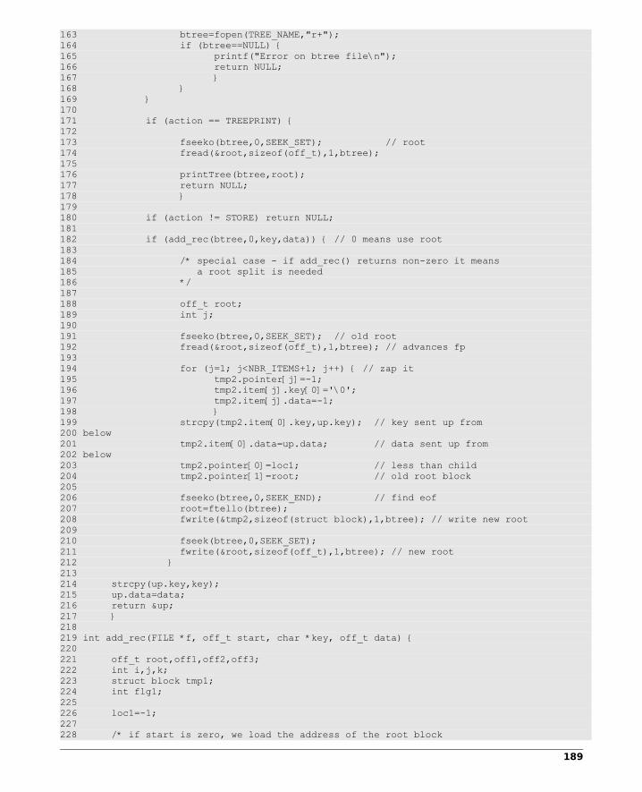
163 btree=fopen(TREE_NAME,"r+");164 if (btree==NULL) {165 printf("Error on btree file\n");166 return NULL;167 }168 }169 }170 171 if (action == TREEPRINT) {172 173 fseeko(btree,0,SEEK_SET); // root174 fread(&root,sizeof(off_t),1,btree); 175 176 printTree(btree,root);177 return NULL;178 }179 180 if (action != STORE) return NULL;181 182 if (add_rec(btree,0,key,data)) { // 0 means use root183 184 /* special case - if add_rec() returns non-zero it means185 a root split is needed 186 */187 188 off_t root;189 int j;190 191 fseeko(btree,0,SEEK_SET); // old root192 fread(&root,sizeof(off_t),1,btree); // advances fp193 194 for (j=1; j<NBR_ITEMS+1; j++) { // zap it195 tmp2.pointer[j]=-1;196 tmp2.item[j].key[0]='\0';197 tmp2.item[j].data=-1;198 }199 strcpy(tmp2.item[0].key,up.key); // key sent up from 200 below201 tmp2.item[0].data=up.data; // data sent up from202 below203 tmp2.pointer[0]=loc1; // less than child204 tmp2.pointer[1]=root; // old root block205 206 fseeko(btree,0,SEEK_END); // find eof207 root=ftello(btree);208 fwrite(&tmp2,sizeof(struct block),1,btree); // write new root209 210 fseek(btree,0,SEEK_SET);211 fwrite(&root,sizeof(off_t),1,btree); // new root 212 }213 214 strcpy(up.key,key);215 up.data=data;216 return &up;217 }218 219 int add_rec(FILE *f, off_t start, char *key, off_t data) {220 221 off_t root,off1,off2,off3;222 int i,j,k;223 struct block tmp1;224 int flg1;225 226 loc1=-1;227 228 /* if start is zero, we load the address of the root block

189

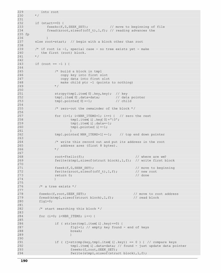
229 into root 230 */231 232 if (start==0) { 233 fseeko(f,0,SEEK_SET); // move to beginning of file234 fread(&root,sizeof(off_t),1,f); // reading advances the 235 fp236 }237 else root=start; // begin with a block other than root238 239 /* if root is -1, special case - no tree exists yet - make240 the first (root) block.241 */242 243 if (root == -1 ) {244 245 /* build a block in tmp1246 copy key into first slot247 copy data into first slot248 make child ptr -1 (points to nothing)249 */250 251 strcpy(tmp1.item[0].key,key); // key252 tmp1.item[0].data=data; // data pointer253 tmp1.pointer[0]=-1; // child254 255 /* zero-out the remainder of the block */256 257 for (i=1; i<NBR_ITEMS+1; i++) { // zero the rest258 tmp1.item[i].key[0]='\0';259 tmp1.item[i].data=-1;260 tmp1.pointer[i]=-1;261 }262 tmp1.pointer[NBR_ITEMS+1]=-1; // top end down pointer263 264 /* write this record out and put its address in the root265 address ares (first 8 bytes).266 */267 268 root=ftello(f); // where are we?269 fwrite(&tmp1,sizeof(struct block),1,f); // write first block270 271 fseek(f,0,SEEK_SET); // move to beginning272 fwrite(&root,sizeof(off_t),1,f); // new root273 return 0; // done274 }275 276 /* a tree exists */277 278 fseeko(f,root,SEEK_SET); // move to root address279 fread(&tmp1,sizeof(struct block),1,f); // read block280 flg1=0;281 282 /* start searching this block */283 284 for (i=0; i<NBR_ITEMS; i++) {285 286 if ( strlen(tmp1.item[i].key)==0) {287 flg1=1; // empty key found - end of keys288 break;289 }290 291 if ( (j=strcmp(key,tmp1.item[i].key)) == 0 ) { // compare keys292 tmp1.item[i].data=data; // found - just update data pointer293 fseeko(f,root,SEEK_SET);294 fwrite(&tmp1,sizeof(struct block),1,f);

190

295 return 0; // done296 }297 298 if (j>0) continue; // search key greater than recorded key299 break; // search key less than recorded key300 // not in this block301 }302 303 if (tmp1.pointer[i]>=0) { // lower block exists - descend304 if ( add_rec(f,tmp1.pointer[i],key,data)==0 ) // key was sent up305 return 0; // finished - no key sent up.306 strcpy(key,up.key); // a split occurred below and this key was sent up307 data=up.data; // data pointer sent up308 }309 310 // insert into long block - block has one extra slot311 312 for (j=NBR_ITEMS; j>=i; j--) { // shift to create opening313 tmp1.pointer[j]=tmp1.pointer[j-1];314 tmp1.item[j]=tmp1.item[j-1];315 }316 317 tmp1.pointer[i]=loc1; // child ptr - zero or sent from below318 strcpy(tmp1.item[i].key,key); // key being added319 tmp1.item[i].data=data; // data being added320 321 for (k=0; k<NBR_ITEMS+1; k++) 322 if (strlen(tmp1.item[k].key)==0) break; // find end of block (k)323 324 if (k<NBR_ITEMS) { // easy insert - block had space325 fseeko(f,root,SEEK_SET);326 fwrite(&tmp1,sizeof(struct block),1,f);327 return 0; // block ok328 }329 330 // split block - block full331 332 333 strcpy(up.key,tmp1.item[NBR_ITEMS/2].key); // key to be sent up334 up.data=tmp1.item[NBR_ITEMS/2].data; // data to be sent up335 336 // tmp2 will be the low order block resulting from the split337 338 for (j=0; j <= NBR_ITEMS/2; j++) { // copy low order data from tmp1339 340 tmp2.pointer[j]=tmp1.pointer[j];341 tmp2.item[j]=tmp1.item[j]; // structure copy342 }343 344 for (j = NBR_ITEMS/2+1; j < NBR_ITEMS+1; j++) { // zap the remainder345 tmp2.pointer[j]=-1;346 tmp2.item[j].key[0]='\0';347 tmp2.item[j].data=-1;348 }349 350 tmp2.item[NBR_ITEMS/2].key[0]=0;351 tmp2.item[NBR_ITEMS/2].data=-1;352 353 fseeko(f,0,SEEK_END); // advance to endfile and record location354 loc1=ftello(f);355 356 fwrite(&tmp2,sizeof(struct block),1,f); // write low block out357 358 // tmp1 is the high order block resulting from the split359 360 for (j=0; j<NBR_ITEMS/2; j++) { // shift its contents down to beginning

191

361 tmp1.pointer[j]=tmp1.pointer[NBR_ITEMS/2+j+1];362 tmp1.item[j]=tmp1.item[NBR_ITEMS/2+j+1];363 }364 365 for (j=NBR_ITEMS/2; j<NBR_ITEMS+1; j++) { // zap its high items366 tmp1.pointer[j]=-1;367 tmp1.item[j].key[0]='\0';368 tmp1.item[j].data=-1;369 }370 371 tmp1.pointer[NBR_ITEMS/2+1]=tmp1.pointer[NBR_ITEMS+1]; // move high end child ptr372 tmp1.pointer[NBR_ITEMS+1]=-1; // zap it373 tmp1.item[NBR_ITEMS+1],key[0]=0; // zap it374 fseeko(f,root,SEEK_SET);375 fwrite(&tmp1,sizeof(struct block),1,f); // write high half376 return 1; // key/data/child ptr being sent up377 }378 379 struct entry * search(FILE * f, char *key, off_t root) {380 381 off_t off1,off2,off3;382 int i,j;383 static struct block tmp1;384 int flg1;385 386 MAX++;387 388 if (root==0) {389 fseeko(f,0,SEEK_SET);390 fread(&root,sizeof(off_t),1,f); // advances fp391 }392 393 fseeko(f,root,SEEK_SET);394 fread(&tmp1,sizeof(struct block),1,f);395 flg1=0;396 for (i=0; i<NBR_ITEMS; i++) {397 398 if ( strlen(tmp1.item[i].key)==0) { flg1=1; break; } 399 // empty key400 401 if ( (j=strcmp(key,tmp1.item[i].key)) == 0 ) {402 return &tmp1.item[i];403 }404 if (j>0) continue;405 break;406 }407 408 if (tmp1.pointer[i]>=0) { // descend - may be high key409 root=tmp1.pointer[i];410 return search(f,key,root);411 }412 return NULL;413 }414 415 void dump(char * cap, FILE *f,off_t root) {416 struct block tmp;417 int i;418 fseeko(f,root,SEEK_SET);419 fread(&tmp,sizeof(struct block),1,f);420 printf("***dump=%s from block nbr %lld\n",cap,root);421 for (i=0; i<NBR_ITEMS+1; i++) {422 printf("%d key=%s %lld423 %lld\n",i,tmp.item[i].key,tmp.item[i].data,tmp.pointer[i]);424 }425 return;426 }

192

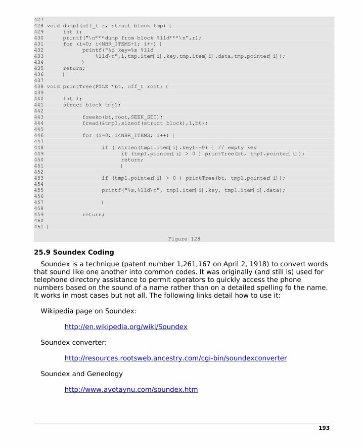
427 428 void dump1(off_t r, struct block tmp) {429 int i;430 printf("\n***dump from block %lld***\n",r);431 for (i=0; i<NBR_ITEMS+1; i++) {432 printf("%d key=%s %lld 433 %lld\n",i,tmp.item[i].key,tmp.item[i].data,tmp.pointer[i]);434 }435 return;436 }437 438 void printTree(FILE *bt, off_t root) {439 440 int i;441 struct block tmp1;442 443 fseeko(bt,root,SEEK_SET);444 fread(&tmp1,sizeof(struct block),1,bt);445 446 for (i=0; i<NBR_ITEMS; i++) {447 448 if ( strlen(tmp1.item[i].key)==0) { // empty key449 if (tmp1.pointer[i] > 0 ) printTree(bt, tmp1.pointer[i]);450 return;451 }452 453 if (tmp1.pointer[i] > 0 ) printTree(bt, tmp1.pointer[i]);454 455 printf("%s,%lld\n", tmp1.item[i].key, tmp1.item[i].data);456 457 }458 459 return;460 461 }

Figure 128

25.9 Soundex Coding

Soundex is a technique (patent number 1,261,167 on April 2, 1918) to convert words that sound like one another into common codes. It was originally (and still is) used for telephone directory assistance to permit operators to quickly access the phone numbers based on the sound of a name rather than on a detailed spelling fo the name. It works in most cases but not all. The following links detail how to use it:

Wikipedia page on Soundex:

http://en.wikipedia.org/wiki/Soundex

Soundex converter:

http://resources.rootsweb.ancestry.com/cgi-bin/soundexconverter

Soundex and Geneology

http://www.avotaynu.com/soundex.htm

193

25.10 MD5 - Message Digest Algorithm 5

MD5 is a cryptographic hash function

Wikipedia page:

http://en.wikipedia.org/wiki/MD5

194

26 References

Altschul, Stephen F., Thomas L. Madden, Alejandro A. Schäffer, Jinghui Zhang, Zheng Zhang, Webb Miller, and David J. Lipman (1997). "Gapped BLAST and PSI-BLAST: a new generation of protein database search programs", Nucleic Acids Res., 25, 3389-3402.

Altschul SF, Gish W, Miller W, Myers EW, Lipman DJ., Basic local alignment search tool. J. Mol. Biol. 215:403-10 (1990).

American National Standards Institute, Inc. (1995). ANSI/MDC X11.4.1995 Information Systems. Programming Languages - M, American National Standards Institute, 11 West 42nd Street, New York, New York 10036.

Baeza-Yates, R. & Ribeiro-Neto, B. (1999). Modern Information Retrieval, Addison-Wesley (Reading, Massachusetts 1999).

http://www.sims.berkeley.edu/~hearst/irbook/10/chap10.html

Blair 1996 Blair, D.C., STAIRS Redux: Thoughts on the STAIRS Evaluation, Ten Years after, Journal American Society for Information Science, Vol 47, No. 1, pp 2-22 (1996).

http://yunus.hacettepe.edu.tr/~tonta/courses/spring2008/bby703/Blair.pdf

Barker, W.C., et. al. (1999). The PIR-International Sequence Database, Nucleic Acids Research, 27(1) 39-43.

Barnett, G.O., & Greenes, R.A. (1970). High level programming languages, Computers and Biomedical Research, 3, 488.497.

Bowie, J., & and Barnett, G. O. (1976). MUMPS . an economical and efficient time-sharing language for information management, Computer Programs in Biomedicine, 6, 11.21.

Frakes, W.B; and Baeza-Yates, R.; Information Retrieval, Data Structures and Algorithms, Prentice-Hall (Englewood Cliffs, NJ 1992).

Heaps, H.S., Information Retrieval, Computational and Theoretical Aspects, Academic Press (New York 1978).

Korfage, R., Information Storage and Retrieval, Wiley (New York, 1997).

Kowalski, G.; and Maybury, M., Information Storage and Retrieval Systems, Theory and Implementation, Second Edition, Kluwer (Boston, 2000).

http://nlp.stanford.edu/IR-book/information-retrieval-book.html

[Manning 2008] Manning, C.; Raghavan, P.; and Schütze, H., Introduction to Information Retrieval, Cambridge University Press (Cambridge 2008).

[Salton, 1968] Salton, G., Automatic Information Organization and Retrieval, McGraw Hill (New York, 1968).

195

[Salton 1971] Salton, G, ed.; The SMART Retrieval System, Experiments in Automatic Document Processing, Prentice-Hall (Englewood Cliffs, NJ, 1971).

[Salton & McGill, 1993] Salton, G.; and McGill, M.J., Introduction to Modern Information Retrieval, McGraw Hill; (New York, 1983).

[Salton, 1988] Salton, G., Automatic Text Processing, Addison-Wesley (Reading, 1988).

[Salton 1992] Salton, G., The state of retrieval system evaluation, Information Processing & Management, 28(4): 441-449; 1992.

[Hersh, 1994] Hersh WR, Buckley C, Leone TJ, Hickam DH, OHSUMED: An interactive retrieval evaluation and new large test collection for research, Proceedings of the 17th Annual ACM SIGIR Conference, 1994, 192-201.

[Hersh 1994] Hersh WR, Hickam DH, Use of a multi-application computer workstation in a clinical setting, Bulletin of the Medical Library Association, 1994, 82: 382-389.

van RIJSBERGEN, C., Information Retrieval

http://www.dcs.gla.ac.uk/Keith/Preface.html

196

Alphabetical IndexAdenine.................................................................................................................................................................10American Society of Indexers...............................................................................................................................63Apache................................................................................................................................................................173ASCII......................................................................................................................................................................17B-tree....................................................................................................................................................................45Bartlett's Familiar Quotations...............................................................................................................................64Bash....................................................................................................................................................................100BigTable................................................................................................................................................................16Bioinformatics.......................................................................................................................................................10Bit Maps................................................................................................................................................................15BLAST............................................................................................................................................................10, 146Boolean logic.........................................................................................................................................................50Building a Stop List...............................................................................................................................................73Caché....................................................................................................................................................................13Cassandra.............................................................................................................................................................16Centroid approximation........................................................................................................................................93Centroid vector.....................................................................................................................................................93Cgi-bin.................................................................................................................................................................174Chmod...................................................................................................................................................................37Clustering......................................................................................................................................................79, 129Coded Tuples........................................................................................................................................................15Cohesion..............................................................................................................................................................126Collating sequence................................................................................................................................................17Concordance.........................................................................................................................................................64Configuring Apache and PHP..............................................................................................................................173Controlled vocabulary.....................................................................................................................................24, 61Cosine.........................................................................................................................................................108, 135Crouch...................................................................................................................................................................92Cytosine................................................................................................................................................................10Database Compression.........................................................................................................................................45Debian...................................................................................................................................................................37DIALOG..................................................................................................................................................................51Dictionary..............................................................................................................................................................64Discrimination Coefficients...................................................................................................................................91Discriminator.........................................................................................................................................................92DNA.......................................................................................................................................................................10Document hyperspace..........................................................................................................................................77Document vectors.................................................................................................................................................77Document-Document..........................................................................................................................................127Document-term matrix.........................................................................................................................................83Dynamo.................................................................................................................................................................16Education Resources Information Center.............................................................................................................55EMBOSS...............................................................................................................................................................147ERIC.......................................................................................................................................................................55FASTA..................................................................................................................................................................147Fdisk....................................................................................................................................................................172Fidelity National Information Systems..................................................................................................................13Frequency of co-occurrence................................................................................................................................116GenBank......................................................................................................................................................145, 148Genetic and protein databases...........................................................................................................................145Genomic databases.............................................................................................................................................147GET........................................................................................................................................................................38GPL........................................................................................................................................................................13GT.M......................................................................................................................................................................13Guanine.................................................................................................................................................................10Hierarchical indexing............................................................................................................................................16HTML...............................................................................................................................................................36, 42IBM DB2.................................................................................................................................................................16IBM IMS .................................................................................................................................................................16

197

IBM STAIRS............................................................................................................................................................51ICD9-CM................................................................................................................................................................62IDF.........................................................................................................................................................................89Index Medicus.......................................................................................................................................................52Index.html...........................................................................................................................................................173Indices...................................................................................................................................................................16Indirection.............................................................................................................................................................24International Union for Pure and Applied Chemistry............................................................................................63InterSystems.........................................................................................................................................................13Inverse Document Frequency...............................................................................................................................89Inverse Document Frequency weight...................................................................................................................89Inverse Document Frequency Weight...................................................................................................................89Inverted file...........................................................................................................................................................50Inverted index.................................................................................................................................................42, 49IUPAC.....................................................................................................................................................................63Jaccard...................................................................................................................................................................81JOSS.......................................................................................................................................................................13King James Bible....................................................................................................................................................64KWAC.....................................................................................................................................................................69KWIC......................................................................................................................................................................69KWOC....................................................................................................................................................................69Library of Congress Classification System............................................................................................................63Linux......................................................................................................................................................................13Lockheed...............................................................................................................................................................51Luhn......................................................................................................................................................................68MARBL.................................................................................................................................................................147MCA.................................................................................................................................................................88, 93MD5.....................................................................................................................................................................195Medical Subject Headings.....................................................................................................................................23MEDLARS.........................................................................................................................................................52, 55MEDLINE..........................................................................................................................................................20, 42MeSH.........................................................................................................................................................23, 42, 62Microsoft SQL Server.............................................................................................................................................16Modified centroid algorithm..................................................................................................................................92Modified Centroid Algorithm...........................................................................................................................88, 92Multi-dimensional..................................................................................................................................................16Mumps...................................................................................................................................................................13MySQL...................................................................................................................................................................16National Center for Biotechnology Information............................................................................................10, 145National Institute for Standards and Technology.................................................................................................19National Library of Medicine...........................................................................................................................23, 52National Library of Medicine Classification Schedule...........................................................................................63Natural language queries......................................................................................................................................57NCBI........................................................................................................................................................10, 55, 145NIST.......................................................................................................................................................................19NLM.................................................................................................................................................................23, 52Nohup..................................................................................................................................................................100NoSQL....................................................................................................................................................................16Null dictionary.......................................................................................................................................................72Optimum Binary Tree..................................................................................................................................181, 184Oracle RDBMS.......................................................................................................................................................16Parallel execution..................................................................................................................................................66Pipe.......................................................................................................................................................................65POST......................................................................................................................................................................38PostgreSQL............................................................................................................................................................16Precision................................................................................................................................................................58Probabilistic scoring..............................................................................................................................................57Public_html..........................................................................................................................................................173PubMed...........................................................................................................................................................52, 55Query vector...........................................................................................................................................79, 97, 108QUERY_STRING.....................................................................................................................................39, 100, 135RAID 0.................................................................................................................................................................172Ranking.................................................................................................................................................................51RDBMS...................................................................................................................................................................16Recall.....................................................................................................................................................................58

198

Relational Database Management System...........................................................................................................16Resolving power....................................................................................................................................................68Salton..............................................................................................................................................................14, 77Smith-Waterman.................................................................................................................................................148Sort...............................................................................................................................................................46p., 66Soundex..............................................................................................................................................................194Sparse...................................................................................................................................................................16Sparse arrays........................................................................................................................................................16SQL........................................................................................................................................................................15Stop list.................................................................................................................................................................72Stop.dat.................................................................................................................................................................72Structural Classification of Proteins......................................................................................................................63Su..........................................................................................................................................................................37Sudo......................................................................................................................................................................37Term connection matrix......................................................................................................................................116Term Discrimination..............................................................................................................................................92Term Discrimination weight..................................................................................................................................88Term Phrases......................................................................................................................................................126Term-document matrix......................................................................................................................................97p.Term-Term clustering..........................................................................................................................................124Term-term correlation.........................................................................................................................................114Term-term correlation matrix.............................................................................................................................116Term-term matrix.......................................................................................................................................116, 124Text REtrieval Conferences...................................................................................................................................19Thesaurus............................................................................................................................................................114Thesaurus construction.......................................................................................................................................114Thymine................................................................................................................................................................10Transpose............................................................................................................................................................115TREC......................................................................................................................................................................19TREC-9...................................................................................................................................................................19TREC-9 Filtering Track...........................................................................................................................................19Tymnet..................................................................................................................................................................55Ubuntu..........................................................................................................................................................37, 173Uncontrolled vocabulary.......................................................................................................................................61Uniq.......................................................................................................................................................................66Vector Space Model..............................................................................................................................................77Very high frequency..............................................................................................................................................72Very low frequency...............................................................................................................................................72Web Page Access................................................................................................................................................133Word frequency list...............................................................................................................................................74WordNet................................................................................................................................................................70Xecute...................................................................................................................................................................25Yahoo....................................................................................................................................................................63Zipf's Law..............................................................................................................................................................66 Cosine...................................................................................................................................................................80 Dice......................................................................................................................................................................81 IBM STAIRS...........................................................................................................................................................50 OSU MEDLINE Data Base.....................................................................................................................................19@...........................................................................................................................................................................32<FORM>.........................................................................................................................................................38, 40<INPUT>...............................................................................................................................................................38$data()...................................................................................................................................................................17$find()....................................................................................................................................................................34$ftell()....................................................................................................................................................................43$order().................................................................................................................................................................17$qlength()..............................................................................................................................................................34$qsubscript().........................................................................................................................................................30$query()....................................................................................................................................................30, 32, 34$zBlanks................................................................................................................................................................64$zdump()...............................................................................................................................................................45$zgetenv...............................................................................................................................................................83$zlower..................................................................................................................................................................64$zNoBlanks............................................................................................................................................................64$znormal...............................................................................................................................................................64$zrestore().............................................................................................................................................................45

199

$zstem...................................................................................................................................................................64$zzScan.................................................................................................................................................................64$zzScanAlnum.......................................................................................................................................................64$zzTranspose........................................................................................................................................................97

200