CSC2541 Lecture 1 Introduction - GitHub Pages · Bring a draft presentation to o ce hours. Roger...

CSC2541 Lecture 1Introduction

Roger Grosse

Roger Grosse CSC2541 Lecture 1 Introduction 1 / 36

Motivation

Recent success stories of machine learning, and neural nets inparticular

But our algorithms still struggle with a decades-old problem: knowingwhat they don’t know


Motivation

Why model uncertainty?Confidence calibration: know how reliable a prediction is (e.g. so it can aska human for clarification)

Regularization: prevent your model from overfittingEnsembling: smooth your predictions by averaging them over multiplepossible modelsModel selection: decide which of multiple plausible models best describesthe dataSparsification: drop connections, encode them with fewer bitsExploration

Active learning: decide which training examples are worth labelingBandits: improve the performance of a system where the feedbackactually counts (e.g. ad targeting)Bayesian optimization: optimize an expensive black-box functionModel-based reinforcement learning (potential orders-of-magnitudegain in sample efficiency!)

Adversarial robustness: make good predictions when the data might have

been perturbed by an adversary


Motivation

Why model uncertainty?Confidence calibration: know how reliable a prediction is (e.g. so it can aska human for clarification)Regularization: prevent your model from overfitting

Ensembling: smooth your predictions by averaging them over multiplepossible modelsModel selection: decide which of multiple plausible models best describesthe dataSparsification: drop connections, encode them with fewer bitsExploration





Motivation

Why model uncertainty?Confidence calibration: know how reliable a prediction is (e.g. so it can aska human for clarification)Regularization: prevent your model from overfittingEnsembling: smooth your predictions by averaging them over multiplepossible models

Model selection: decide which of multiple plausible models best describesthe dataSparsification: drop connections, encode them with fewer bitsExploration





Motivation

Why model uncertainty?Confidence calibration: know how reliable a prediction is (e.g. so it can aska human for clarification)Regularization: prevent your model from overfittingEnsembling: smooth your predictions by averaging them over multiplepossible modelsModel selection: decide which of multiple plausible models best describesthe data

Sparsification: drop connections, encode them with fewer bitsExploration





Motivation

Why model uncertainty?Confidence calibration: know how reliable a prediction is (e.g. so it can aska human for clarification)Regularization: prevent your model from overfittingEnsembling: smooth your predictions by averaging them over multiplepossible modelsModel selection: decide which of multiple plausible models best describesthe dataSparsification: drop connections, encode them with fewer bits

Exploration





Motivation

Why model uncertainty?Confidence calibration: know how reliable a prediction is (e.g. so it can aska human for clarification)Regularization: prevent your model from overfittingEnsembling: smooth your predictions by averaging them over multiplepossible modelsModel selection: decide which of multiple plausible models best describesthe dataSparsification: drop connections, encode them with fewer bitsExploration





Course Overview

Weeks 2–3: Bayesian function approximation

Bayesian neural netsGaussian processes

Weeks 4–5: variational inference

Weeks 6–8: using uncertainty to drive exploration

Weeks 9–10: other topics (adversarial robustness, optimization)

Weeks 11–12: project presentations


What we Don’t Cover

Uncertainty in ML is way too big a topic for one course.

Focus on uncertainty in function approximation, and its use indirecting exploration and improving generalization.

How this differs from other courses

No generative models or discrete Bayesian models (covered in otheriterations of 2541)CSC412, STA414, and ECE521 are core undergrad courses giving broadcoverage of probabilistic modeling.

We cover fewer topics in more depth, and more cutting edge research.

This is an ML course, not a stats course.

Lots of overlap, but problems are motivated by use in AI systems ratherthan human interpretability.


Adminis-trivia: Presentations

10 lectures

Each one covers about 4–6 papers.

I will give 3 (including this one).

The remaining 7 will be student presentations.

8–12 presenters per lecture (signup procedure to be announced soon)Divide lecture into sub-topics on an ad-hoc basisAim for a total of about 75 minutes plus questions/discussionI will send you advice roughly 2 weeks in advanceBring a draft presentation to office hours.


Adminis-trivia: Projects

Goal: write a workshop-quality paper related to the course topics

Work in groups of 3–5

Types of projectsTutorial/review article.

Must have clear value-added: explain the relationship between differentalgorithms, come up with illustrative examples, run experiments on toyproblems, etc.

Apply an existing algorithm in a new setting.Invent a new algorithm.

You’re welcome to do something related to your research (seehandout for detailed policies)

Full information:https://csc2541-f17.github.io/project-handout.pdf


https://csc2541-f17.github.io/project-handout.pdf

Adminis-trivia: Projects

Project proposal (due Oct. 12)

about 2 pagesdescribe motivation, related work

Presentations (Nov. 24 and Dec. 1)

Each group has 5 minutes + 2 minutes for questions.

Final report (due Dec. 10)

about 8 pages plus references (not strictly enforced)submit code also

See handout for specific policies.


Adminis-trivia: Marks

Class presentations — 20%

Project Proposal — 20%

Projects — 60%

85% (A-/A) for meeting requirements, last 15% for going above andbeyondSee handout for specific requirements and breakdown


History of Bayesian Modeling

1763 — Bayes’ Rule published (further developed by Laplace in 1774)

1953 — Metropolis algorithm (extended by Hastings in 1970)

1984 — Stuart and Donald Geman invent Gibbs sampling (moregeneral statistical formulation by Gelfand and Smith in 1990)

1990s — Hamiltonian Monte Carlo

1990s — Bayesian neural nets and Gaussian processes

1990s — probabilistic graphical models

1990s — sequential Monte Carlo

1990s — variational inference

1997 — BUGS probabilistic programming language

2000s — Bayesian nonparametrics

2010 — stochastic variational inference

2012 — Stan probabilistic programming language


History of Neural Networks

1949 — Hebbian learning (“fire together, wire together”)

1957 — perceptron algorithm

1969 — Minsky and Papert’s book Perceptrons (limitations of linearmodels)

1982 — Hopfield networks (model of associative memory)

1988 — backpropagation

1989 — convolutional networks

1990s — neural net winter

1997 — long-term short-term memory (LSTM) (not appreciated untillast few years)

2006 — “deep learning”

2010s — GPUs

2012 — AlexNet smashes the ImageNet object recognitionbenchmark, leading to the current deep learning boom

2016 — AlphaGo defeats human Go champion


This Lecture

confidence calibration

intro to Bayesian modeling: coin flip example

n-armed bandits and exploration

Bayesian linear regression


Calibration

Calibration: of the times your model predicts something with 90%confidence, is it right 90% of the time?

From Nate Silver’s book, “The Signal and the Noise”: calibration ofweather forecasts

The Weather Channel local weather station


Calibration

Most of our neural nets output probability distributions, e.g. overobject categories. Are these calibrated?From Guo et al. (2017):


Calibration

Suppose an algorithm outputs a probability distribution over targets,and gets a loss based on this distribution and the true target.

A proper scoring rule is a scoring rule where the algorithm’s beststrategy is to output the true distribution.

The canonical example is negative log-likelihood (NLL). If k is thecategory label, t is the indicator vector for the label, and y are thepredicted probabilities,

L(y, t) = − log yk = −t>(log y)


Calibration

Calibration failures show up in the test NLL scores:

— Guo et al., 2017, On calibration of modern neural networks


Calibration

Guo et al. explored 7 different calibration methods, but the one thatworked the best was also the simplest: temperature scaling.

A classification network typically predicts σ(z), where σ is thesoftmax function

σ(z)k =exp(zk)∑k ′ exp(zk ′)

and z are called the logits.

They replace this withσ(z/T ),

where T is a scalar called the temperature.

T is tuned to minimize the NLL on a validation set.

Intuitively, because NLL is a proper scoring rule, the algorithm isincentivized to match the true probabilities as closely as possible.


Calibration

Before and after temperature scaling:


A Toy Example

Thomas Bayes, “An Essay towards Solving a Problem in the Doctrine of Chances.”

Philosophical Transactions of the Royal Society, 1763.


A Toy Example

Motivating example: estimating the parameter of a biased coin

You flip a coin 100 times. It lands heads NH = 55 times and tailsNT = 45 times.What is the probability it will come up heads if we flip again?

Model: observations xi are independent and identically distributed(i.i.d.) Bernoulli random variables with parameter θ.

The likelihood function is the probability of the observed data (theentire sequence of H’s and T’s) as a function of θ:

L(θ) = p(D) =N∏i=1

θxi (1− θ)1−xi

= θNH (1− θ)NT

NH and NT are sufficient statistics.


A Toy Example

The likelihood is generally very small, so it’s often convenient to workwith log-likelihoods.

L(θ) = θNH (1− θ)NT ≈ 7.9× 10−31

`(θ) = log L(θ) = NH log θ + NT log(1− θ) ≈ −69.31


A Toy Example

Good values of θ should assign high probability to the observed data.This motivates the maximum likelihood criterion.

Solve by setting derivatives to zero:

d`

dθ=

d

dθ(NH log θ + NT log(1− θ))

=NH

θ− NT

1− θ

Setting this to zero gives the maximum likelihood estimate:

θ̂ML =NH

NH + NT,

Normally there’s no analytic solution, and we need to solve anoptimization problem (e.g. using gradient descent).


A Toy Example

Maximum likelihood has a pitfall: if you have too little data, it canoverfit.

E.g., what if you flip the coin twice and get H both times?

θML =NH

NH + NT=

2

2 + 0= 1

Because it never observed T, it assigns this outcome probability 0.This problem is known as data sparsity.

If you observe a single T in the test set, the likelihood is −∞.


A Toy Example

In maximum likelihood, the observations are treated as randomvariables, but the parameters are not.

The Bayesian approach treats the parameters as random variables aswell.

To define a Bayesian model, we need to specify two distributions:

The prior distribution p(θ), which encodes our beliefs about theparameters before we observe the dataThe likelihood p(D |θ), same as in maximum likelihood

When we update our beliefs based on the observations, we computethe posterior distribution using Bayes’ Rule:

p(θ | D) =p(θ)p(D |θ)∫

p(θ′)p(D |θ′)dθ′.

We rarely ever compute the denominator explicitly.


A Toy Example

Let’s revisit the coin example. We already know the likelihood:

L(θ) = p(D) = θNH (1− θ)NT

It remains to specify the prior p(θ).

We can choose an uninformative prior, which assumes as little aspossible. A reasonable choice is the uniform prior.But our experience tells us 0.5 is more likely than 0.99. Oneparticularly useful prior that lets us specify this is the beta distribution:

p(θ; a, b) =Γ(a + b)

Γ(a)Γ(b)θa−1(1− θ)b−1.

This notation for proportionality lets us ignore the normalizationconstant:

p(θ; a, b) ∝ θa−1(1− θ)b−1.


A Toy Example

Beta distribution for various values of a, b:

Some observations:

The expectation E[θ] = a/(a + b).The distribution gets more peaked when a and b are large.The uniform distribution is the special case where a = b = 1.

The main thing the beta distribution is used for is as a prior for the Bernoullidistribution.


A Toy Example

Computing the posterior distribution:

p(θ | D) ∝ p(θ)p(D |θ)

∝[θa−1(1− θ)b−1

] [θNH (1− θ)NT

]= θa−1+NH (1− θ)b−1+NT .

This is just a beta distribution with parameters NH + a and NT + b.

The posterior expectation of θ is:

E[θ | D] =NH + a

NH + NT + a + b

The parameters a and b of the prior can be thought of aspseudo-counts.

The reason this works is that the prior and likelihood have the samefunctional form. This phenomenon is known as conjugacy, and it’s veryuseful.


A Toy Example

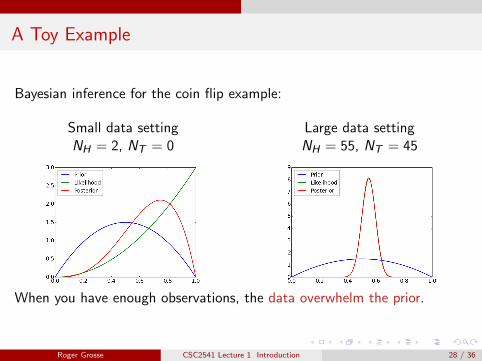
Bayesian inference for the coin flip example:

Small data settingNH = 2, NT = 0

Large data settingNH = 55, NT = 45

When you have enough observations, the data overwhelm the prior.


A Toy Example

What do we actually do with the posterior?

The posterior predictive distribution is the distribution over futureobservables given the past observations. We compute this bymarginalizing out the parameter(s):

p(D′ | D) =

∫p(θ | D)p(D′ |θ) dθ. (1)

For the coin flip example:

θpred = Pr(x′ = H | D)

=

∫p(θ | D)Pr(x′ = H | θ)dθ

=

∫Beta(θ;NH + a,NT + b) · θ dθ

= EBeta(θ;NH+a,NT+b)[θ]

=NH + a

NH + NT + a + b, (2)


A Toy Example

Maximum a-posteriori (MAP) estimation: find the most likelyparameter settings under the posterior

This converts the Bayesian parameter estimation problem into amaximization problem

θ̂MAP = arg maxθ

p(θ | D)

= arg maxθ

p(θ,D)

= arg maxθ

p(θ) p(D |θ)

= arg maxθ

log p(θ) + log p(D |θ)


A Toy Example

Joint probability in the coin flip example:

log p(θ,D) = log p(θ) + log p(D | θ)

= const + (a− 1) log θ + (b − 1) log(1− θ) + NH log θ + NT log(1− θ)

= const + (NH + a− 1) log θ + (NT + b − 1) log(1− θ)

Maximize by finding a critical point

0 =d

dθlog p(θ,D) =

NH + a− 1

θ− NT + b − 1

1− θ

Solving for θ,

θ̂MAP =NH + a− 1

NH + NT + a + b − 2


A Toy Example

Comparison of estimates in the coin flip example:

Formula NH = 2,NT = 0 NH = 55,NT = 45

θ̂MLNH

NH+NT1 55

100 = 0.55

θpredNH+a

NH+NT+a+b46 ≈ 0.67 57

104 ≈ 0.548

θ̂MAPNH+a−1

NH+NT+a+b−234 = 0.75 56

102 ≈ 0.549

θ̂MAP assigns nonzero probabilities as long as a, b > 1.


A Toy Example

Lessons learnedBayesian parameter estimation is more robust to data sparsity.

Not the most spectacular selling point. But stay tuned.

Maximum likelihood is about optimization, while Bayesian parameterestimation is about integration.

Which one is easier?

It’s not (just) about priors.

The Bayesian solution with a uniform prior is robust to data sparsity.Why?

The Bayesian solution converges to the maximum likelihood solution asyou observe more data.

Does this mean Bayesian methods are only useful on small datasets?


Preview: Bandits

Despite its simplicity, the coin flip example is already useful.

n-armed bandit problem: you have n slot machine arms in front ofyou, and each one pays out $1 with an unknown probability θi . Youget T tries, and you’d like to maximize your total winnings.

Consider some possible strategies:

greedy: pick whichever one has paid out the most frequently so farpick the arm whose parameter we are most uncertain aboutε-greedy: do the greedy strategy with probability 1− ε, but pick arandom arm with probability ε

We’d like to balance exploration and exploitation.

Optimism in the face of uncertaintyBandits are a good model of exploration/exploitation for more complexsettings we’ll cover in this course (e.g. Bayesian optimization,reinforcement learning)


Preview: Bandits




greedy: pick whichever one has paid out the most frequently so far

pick the arm whose parameter we are most uncertain aboutε-greedy: do the greedy strategy with probability 1− ε, but pick arandom arm with probability ε




Preview: Bandits




greedy: pick whichever one has paid out the most frequently so farpick the arm whose parameter we are most uncertain about

ε-greedy: do the greedy strategy with probability 1− ε, but pick arandom arm with probability ε




Preview: Bandits




greedy: pick whichever one has paid out the most frequently so farpick the arm whose parameter we are most uncertain aboutε-greedy: do the greedy strategy with probability 1− ε, but pick arandom arm with probability ε




Preview: Bandits

One elegant solution: Thompson sampling (invented in 1933, ignoredin AI until 1990s)

Sample each θi ∼ p(θi | D), and pick the max.

If these are the current posteriors over three arms, which one will itpick next?

— Russo et al., 2017, A tutorial on Thompson sampling


Preview: Bandits

Why does this:

encourage exploration?stop trying really bad actions?emphasize exploration first and exploitation later?

Comparison of exploration methods on a more structured bandit problem

— Russo et al., 2017, A tutorial on Thompson sampling


CSC2541 Lecture 1 Introduction - GitHub Pages · Bring a draft presentation to o ce hours. Roger...

Documents

Transcript of CSC2541 Lecture 1 Introduction - GitHub Pages · Bring a draft presentation to o ce hours. Roger...