CS 7643: Deep Learning - Georgia Institute of Technology 28 28 Slide Credit: Fei-FeiLi, Justin...
69
CS 7643: Deep Learning Dhruv Batra Georgia Tech Topics: – Toeplitz matrices and convolutions = matrix-mult – Dilated/a-trous convolutions – Backprop in conv layers – Transposed convolutions
Transcript of CS 7643: Deep Learning - Georgia Institute of Technology 28 28 Slide Credit: Fei-FeiLi, Justin...

CS 7643: Deep Learning
Dhruv Batra Georgia Tech
Topics: – Toeplitz matrices and convolutions = matrix-mult– Dilated/a-trous convolutions– Backprop in conv layers– Transposed convolutions

Administrativia• HW1 extension
– 09/22 09/25
• HW2 + PS2 both coming out on 09/22 09/25
• Note on class schedule coming up– Switching to paper reading starting next week. – https://docs.google.com/spreadsheets/d/1uN31YcWAG6nhjv
YPUVKMy3vHwW-h9MZCe8yKCqw0RsU/edit#gid=0
• First review due: Tue 09/26
• First student presentation due: Thr 09/28
(C) Dhruv Batra 2

Recap of last time
(C) Dhruv Batra 3
Convolutional Neural Networks(without the brain stuff)
Slide Credit: Fei-Fei Li, Justin Johnson, Serena Yeung, CS 231n

Convolutional Neural Networksa
(C) Dhruv Batra 5
INPUT 32x32
Convolutions SubsamplingConvolutions
C1: feature maps 6@28x28
Subsampling
S2: f. maps6@14x14
S4: f. maps 16@5x5C5: layer120
C3: f. maps 16@10x10
F6: layer 84
Full connectionFull connection
Gaussian connections
OUTPUT 10
Image Credit: Yann LeCun, Kevin Murphy

6
FC vs Conv Layer

32
32
3
Convolution Layer32x32x3 image5x5x3 filter
1 number: the result of taking a dot product between the filter and a small 5x5x3 chunk of the image(i.e. 5*5*3 = 75-dimensional dot product + bias)
Slide Credit: Fei-Fei Li, Justin Johnson, Serena Yeung, CS 231n

32
32
3
Convolution Layer32x32x3 image5x5x3 filter
convolve (slide) over all spatial locations
activation map
1
28
28
Slide Credit: Fei-Fei Li, Justin Johnson, Serena Yeung, CS 231n
32
32
3
Convolution Layer
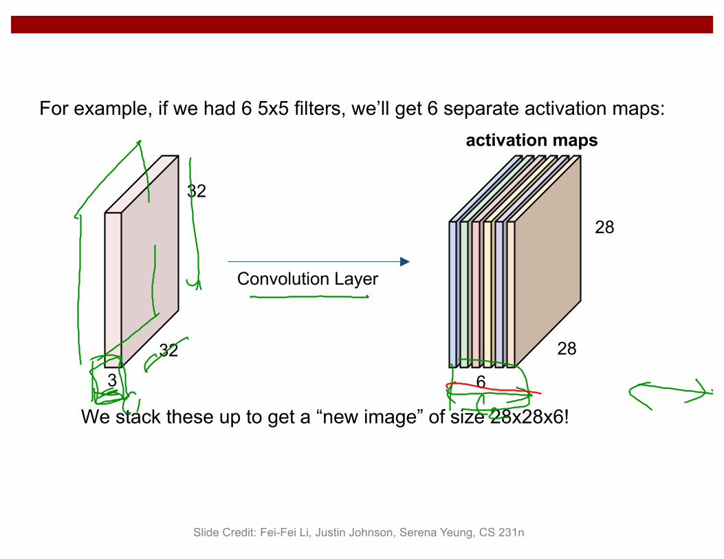
activation maps
6
28
28
For example, if we had 6 5x5 filters, we’ll get 6 separate activation maps:
We stack these up to get a “new image” of size 28x28x6!
Slide Credit: Fei-Fei Li, Justin Johnson, Serena Yeung, CS 231n

Preview: ConvNet is a sequence of Convolutional Layers, interspersed with activation functions
32
32
3
CONV,ReLUe.g. 6 5x5x3 filters 28
28
6
CONV,ReLUe.g. 10 5x5x6 filters
CONV,ReLU
….
1024
24
Slide Credit: Fei-Fei Li, Justin Johnson, Serena Yeung, CS 231n

N
NF
F
Output size:(N - F) / stride + 1
e.g. N = 7, F = 3:stride 1 => (7 - 3)/1 + 1 = 5stride 2 => (7 - 3)/2 + 1 = 3stride 3 => (7 - 3)/3 + 1 = 2.33 :\
Slide Credit: Fei-Fei Li, Justin Johnson, Serena Yeung, CS 231n

In practice: Common to zero pad the border
e.g. input 7x73x3 filter, applied with stride 1 pad with 1 pixel border => what is the output?
7x7 output!in general, common to see CONV layers with stride 1, filters of size FxF, and zero-padding with (F-1)/2. (will preserve size spatially)e.g. F = 3 => zero pad with 1
F = 5 => zero pad with 2F = 7 => zero pad with 3
0 0 0 0 0 0
0
0
0
0
Slide Credit: Fei-Fei Li, Justin Johnson, Serena Yeung, CS 231n

(btw, 1x1 convolution layers make perfect sense)
6456
561x1 CONVwith 32 filters
3256
56(each filter has size 1x1x64, and performs a 64-dimensional dot product)
Slide Credit: Fei-Fei Li, Justin Johnson, Serena Yeung, CS 231n
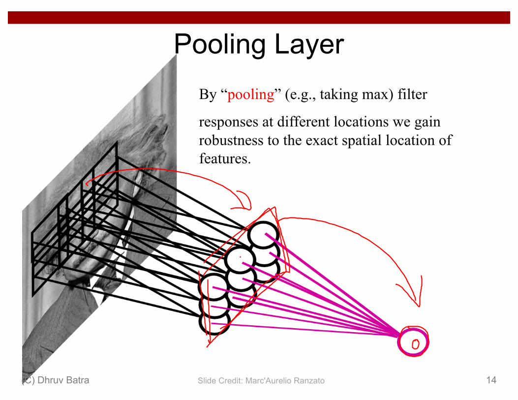
By “pooling” (e.g., taking max) filter
responses at different locations we gain robustness to the exact spatial location of features.
Pooling Layer
Slide Credit: Marc'Aurelio Ranzato(C) Dhruv Batra 14
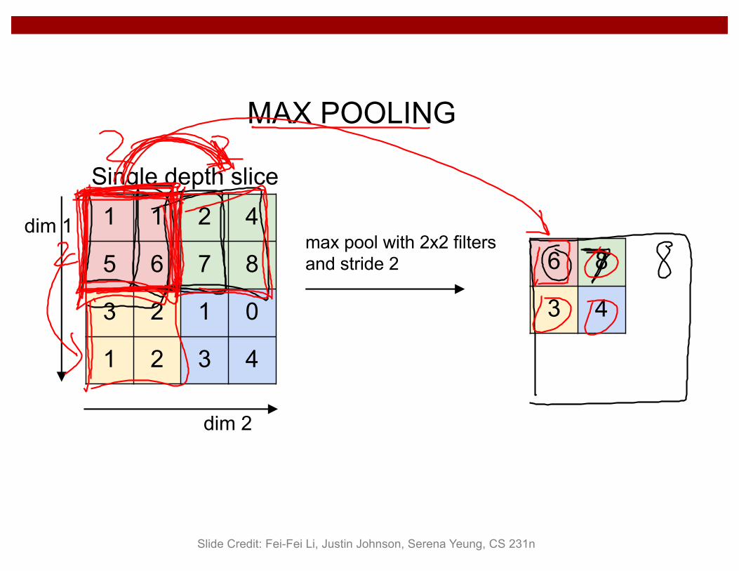
1 1 2 4
5 6 7 8
3 2 1 0
1 2 3 4
Single depth slice
dim 1
dim 2
max pool with 2x2 filters and stride 2 6 8
3 4
MAX POOLING
Slide Credit: Fei-Fei Li, Justin Johnson, Serena Yeung, CS 231n

Max-pooling:
Average-pooling:
L2-pooling:
L2-pooling over features:
Pooling Layer: Examples
Slide Credit: Marc'Aurelio Ranzato(C) Dhruv Batra 16
hni (r, c) = max
r̄2N(r), c̄2N(c)hn�1i (r̄, c̄)
hni (r, c) = mean
r̄2N(r), c̄2N(c)hn�1i (r̄, c̄)
hni (r, c) =
s X
r̄2N(r), c̄2N(c)
hn�1i (r̄, c̄)2
hni (r, c) =
s X
j2N(i)
hn�1i (r, c)2

Classical View
(C) Dhruv Batra 17Figure Credit: [Long, Shelhamer, Darrell CVPR15]

MxMxN, M small
H hidden units
Fully conn. layer
Slide Credit: Marc'Aurelio Ranzato(C) Dhruv Batra 18

Classical View = Inefficient
(C) Dhruv Batra 19

Classical View
(C) Dhruv Batra 20Figure Credit: [Long, Shelhamer, Darrell CVPR15]

Re-interpretation• Just squint a little!
(C) Dhruv Batra 21Figure Credit: [Long, Shelhamer, Darrell CVPR15]

“Fully Convolutional” Networks• Can run on an image of any size!
(C) Dhruv Batra 22Figure Credit: [Long, Shelhamer, Darrell CVPR15]
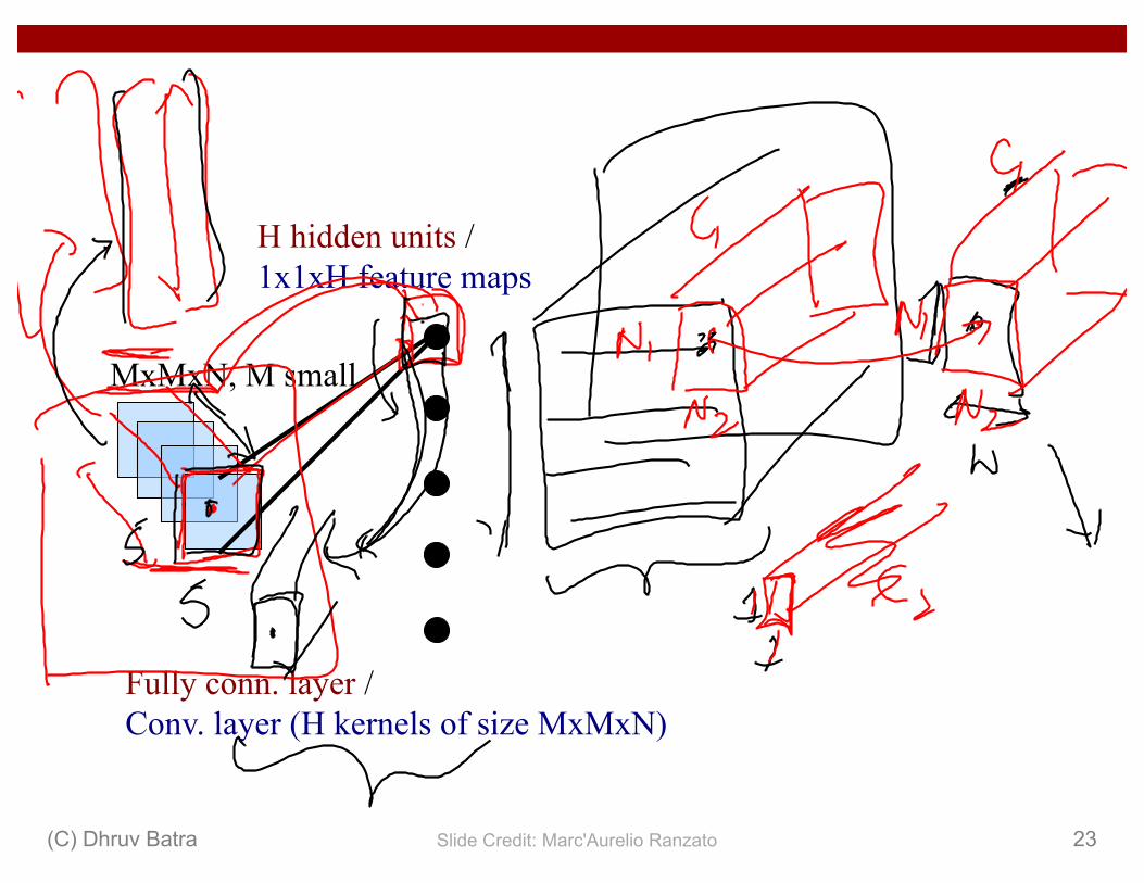
MxMxN, M small
H hidden units / 1x1xH feature maps
Fully conn. layer /Conv. layer (H kernels of size MxMxN)
Slide Credit: Marc'Aurelio Ranzato(C) Dhruv Batra 23

MxMxN, M small
H hidden units / 1x1xH feature maps
Fully conn. layer /Conv. layer (H kernels of size MxMxN)
K hidden units / 1x1xK feature maps
Fully conn. layer /Conv. layer (K kernels of size 1x1xH)
Slide Credit: Marc'Aurelio Ranzato(C) Dhruv Batra 24

Viewing fully connected layers as convolutional layers enables efficient use of convnets on bigger images (no need to slide windows but unroll network over space as needed to re-use computation).
CNNInput
Image
CNNInput
ImageInput
Image
TRAINING TIME
TEST TIME
x
y
Slide Credit: Marc'Aurelio Ranzato(C) Dhruv Batra 25

CNNInput
Image
CNNInput
Image
TRAINING TIME
TEST TIME
x
y
Unrolling is order of magnitudes more eficient than sliding windows!
CNNs work on any image size!
Viewing fully connected layers as convolutional layers enables efficient use of convnets on bigger images (no need to slide windows but unroll network over space as needed to re-use computation).
Slide Credit: Marc'Aurelio Ranzato(C) Dhruv Batra 26

Benefit of this thinking• Mathematically elegant
• Efficiency– Can run network on arbitrary image – Without multiple crops
(C) Dhruv Batra 27

Summary
- ConvNets stack CONV,POOL,FC layers- Trend towards smaller filters and deeper architectures- Trend towards getting rid of POOL/FC layers (just CONV)- Typical architectures look like
[(CONV-RELU)*N-POOL?]*M-(FC-RELU)*K,SOFTMAXwhere N is usually up to ~5, M is large, 0 <= K <= 2.- but recent advances such as ResNet/GoogLeNet
challenge this paradigm
Slide Credit: Fei-Fei Li, Justin Johnson, Serena Yeung, CS 231n

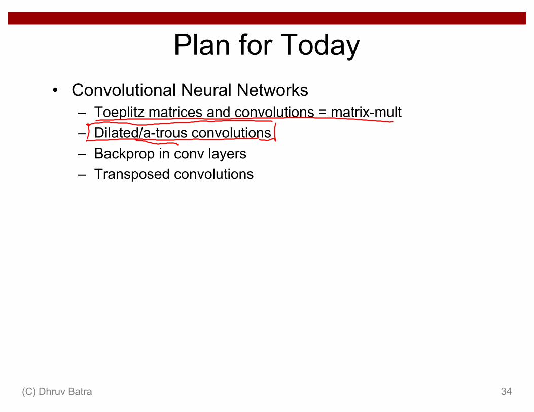
Plan for Today• Convolutional Neural Networks
– Toeplitz matrices and convolutions = matrix-mult– Dilated/a-trous convolutions– Backprop in conv layers– Transposed convolutions
(C) Dhruv Batra 29

Toeplitz Matrix• Diagonals are constants
• Aij = ai-j
(C) Dhruv Batra 30

Why do we care?• (Discrete) Convolution = Matrix Multiplication
– with Toeplitz Matrices
(C) Dhruv Batra 31
y = w ⇤ x
2
66666666666666666664
wk 0 . . . 0 0wk�1 wk . . . 0 0wk�2 wk�1 . . . 0 0...
......
......
w1 wk�2 . . . wk 0...
......
......
0 w1 . . . wk�1 wk...
......
......
0 0... w1 w2
0 0... 0 w1
3
77777777777777777775
2
666664
x1
x2
x3...xn
3
777775

(C) Dhruv Batra 32
"Convolution of box signal with itself2" by Convolution_of_box_signal_with_itself.gif: Brian Ambergderivative work: Tinos (talk) - Convolution_of_box_signal_with_itself.gif. Licensed under CC BY-SA 3.0 via Commons -
https://commons.wikimedia.org/wiki/File:Convolution_of_box_signal_with_itself2.gif#/media/File:Convolution_of_box_signal_with_itself2.gif

(C) Dhruv Batra 33
Plan for Today• Convolutional Neural Networks
– Toeplitz matrices and convolutions = matrix-mult– Dilated/a-trous convolutions– Backprop in conv layers– Transposed convolutions
(C) Dhruv Batra 34

Dilated Convolutions
(C) Dhruv Batra 35

Dilated Convolutions
(C) Dhruv Batra 36

(C) Dhruv Batra 37

(C) Dhruv Batra 38
(recall:)(N - k) / stride + 1

(C) Dhruv Batra 39Figure Credit: Yu and Koltun, ICLR16

Plan for Today• Convolutional Neural Networks
– Toeplitz matrices and convolutions = matrix-mult– Dilated/a-trous convolutions– Backprop in conv layers– Transposed convolutions
(C) Dhruv Batra 40

Backprop in Convolutional Layers
(C) Dhruv Batra 41

Backprop in Convolutional Layers
(C) Dhruv Batra 42
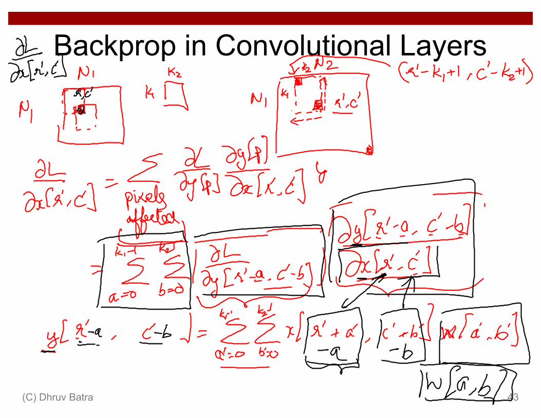
Backprop in Convolutional Layers
(C) Dhruv Batra 43

Backprop in Convolutional Layers
(C) Dhruv Batra 44

Plan for Today• Convolutional Neural Networks
– Toeplitz matrices and convolutions = matrix-mult– Dilated/a-trous convolutions– Backprop in conv layers– Transposed convolutions
(C) Dhruv Batra 45

Transposed Convolutions• Deconvolution (bad)• Upconvolution• Fractionally strided convolution• Backward strided convolution
(C) Dhruv Batra 46

Class ScoresCat: 0.9Dog: 0.05Car: 0.01...
So far: Image Classification
This image is CC0 public domain Vector:4096
Fully-Connected:4096 to 1000
FigurecopyrightAlexKrizhevsky,IlyaSutskever,andGeoffreyHinton,2012.Reproducedwithpermission.
Slide Credit: Fei-Fei Li, Justin Johnson, Serena Yeung, CS 231n

Other Computer Vision TasksClassification + Localization
SemanticSegmentation
Object Detection
Instance Segmentation
CATGRASS, CAT, TREE, SKY
DOG, DOG, CAT DOG, DOG, CAT
Single Object Multiple ObjectNo objects, just pixels This image is CC0 public domain
Slide Credit: Fei-Fei Li, Justin Johnson, Serena Yeung, CS 231n

Semantic Segmentation
Cow
Grass
Sky
Label each pixel in the image with a category label
Don’t differentiate instances, only care about pixels
This image is CC0 public domain
Grass
Cat
Sky
Slide Credit: Fei-Fei Li, Justin Johnson, Serena Yeung, CS 231n

Semantic Segmentation Idea: Sliding Window
Full image
Extract patchClassify center pixel with CNN
Cow
Cow
Grass
Farabet et al, “Learning Hierarchical Features for Scene Labeling,” TPAMI 2013Pinheiro and Collobert, “Recurrent Convolutional Neural Networks for Scene Labeling”, ICML 2014
Slide Credit: Fei-Fei Li, Justin Johnson, Serena Yeung, CS 231n

Semantic Segmentation Idea: Sliding Window
Full image
Extract patchClassify center pixel with CNN
Cow
Cow
GrassProblem: Very inefficient! Not reusing shared features between overlapping patches Farabet et al, “Learning Hierarchical Features for Scene Labeling,” TPAMI 2013
Pinheiro and Collobert, “Recurrent Convolutional Neural Networks for Scene Labeling”, ICML 2014
Slide Credit: Fei-Fei Li, Justin Johnson, Serena Yeung, CS 231n

Semantic Segmentation Idea: Fully Convolutional
Input:3 x H x W
Convolutions:D x H x W
Conv Conv Conv Conv
Scores:C x H x W
argmax
Predictions:H x W
Design a network as a bunch of convolutional layers to make predictions for pixels all at once!
Problem: convolutions at original image resolution will be very expensive ...
Slide Credit: Fei-Fei Li, Justin Johnson, Serena Yeung, CS 231n

Semantic Segmentation Idea: Fully Convolutional
Input:3 x H x W Predictions:
H x W
Design network as a bunch of convolutional layers, with downsampling and upsampling inside the network!
High-res:D1 x H/2 x W/2
High-res:D1 x H/2 x W/2
Med-res:D2 x H/4 x W/4
Med-res:D2 x H/4 x W/4
Low-res:D3 x H/4 x W/4
Long, Shelhamer, and Darrell, “Fully Convolutional Networks for Semantic Segmentation”, CVPR 2015Noh et al, “Learning Deconvolution Network for Semantic Segmentation”, ICCV 2015
Downsampling:Pooling, strided convolution
Upsampling:???
Slide Credit: Fei-Fei Li, Justin Johnson, Serena Yeung, CS 231n

In-Network upsampling: “Unpooling”
1 2
3 4
Input: 2 x 2 Output: 4 x 4
1 1 2 2
1 1 2 2
3 3 4 4
3 3 4 4
Nearest Neighbor
1 2
3 4
Input: 2 x 2 Output: 4 x 4
1 0 2 0
0 0 0 0
3 0 4 0
0 0 0 0
“Bed of Nails”
Slide Credit: Fei-Fei Li, Justin Johnson, Serena Yeung, CS 231n
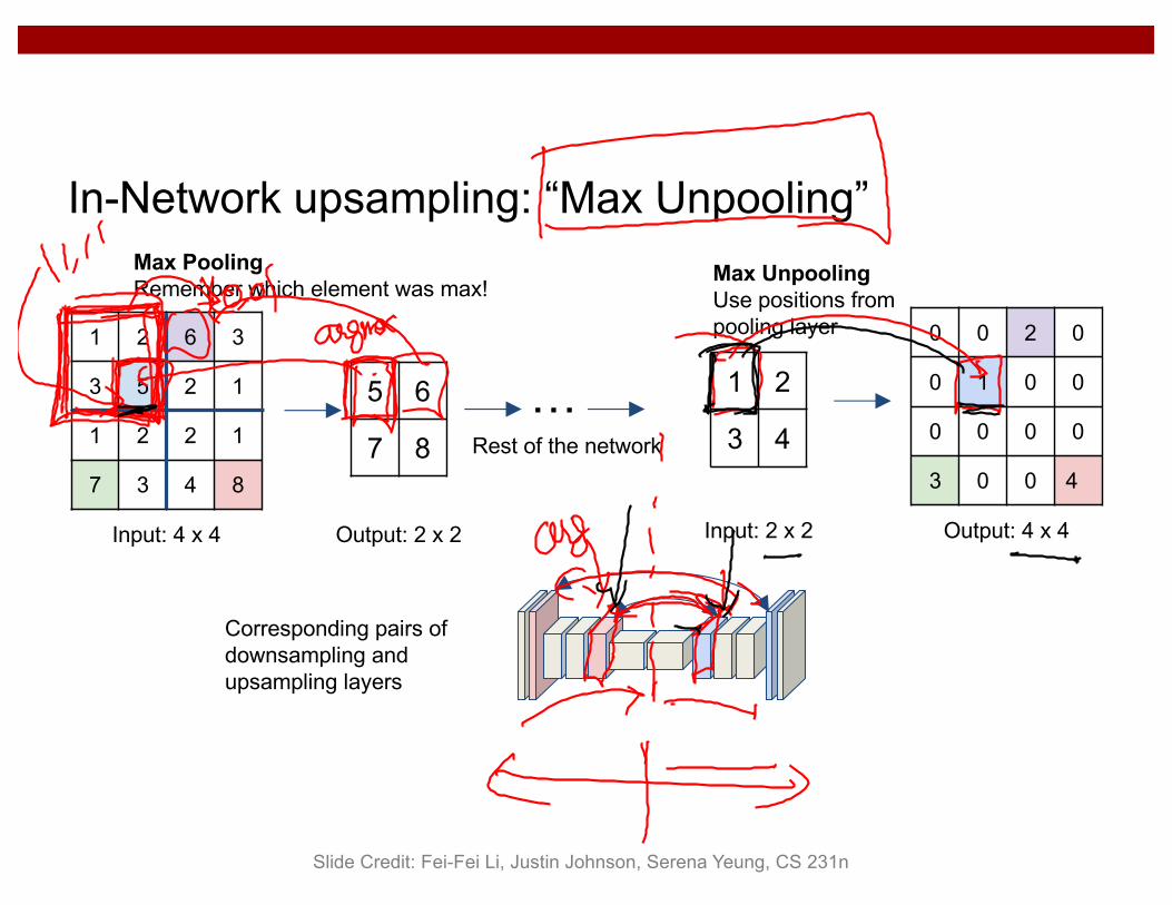
In-Network upsampling: “Max Unpooling”
Input: 4 x 4
1 2 6 3
3 5 2 1
1 2 2 1
7 3 4 8
1 2
3 4
Input: 2 x 2 Output: 4 x 4
0 0 2 0
0 1 0 0
0 0 0 0
3 0 0 4
Max UnpoolingUse positions from pooling layer
5 6
7 8
Max PoolingRemember which element was max!
… Rest of the network
Output: 2 x 2
Corresponding pairs of downsampling and upsampling layers
Slide Credit: Fei-Fei Li, Justin Johnson, Serena Yeung, CS 231n

Learnable Upsampling: Transpose Convolution
Recall:Typical 3 x 3 convolution, stride 1 pad 1
Input: 4 x 4 Output: 4 x 4
Slide Credit: Fei-Fei Li, Justin Johnson, Serena Yeung, CS 231n

Learnable Upsampling: Transpose Convolution
Recall: Normal 3 x 3 convolution, stride 1 pad 1
Input: 4 x 4 Output: 4 x 4
Dot product between filter and input
Slide Credit: Fei-Fei Li, Justin Johnson, Serena Yeung, CS 231n

Learnable Upsampling: Transpose Convolution
Input: 4 x 4 Output: 4 x 4
Dot product between filter and input
Recall: Normal 3 x 3 convolution, stride 1 pad 1
Slide Credit: Fei-Fei Li, Justin Johnson, Serena Yeung, CS 231n

Input: 4 x 4 Output: 2 x 2
Learnable Upsampling: Transpose Convolution
Recall: Normal 3 x 3 convolution, stride 2 pad 1
Slide Credit: Fei-Fei Li, Justin Johnson, Serena Yeung, CS 231n

Input: 4 x 4 Output: 2 x 2
Dot product between filter and input
Learnable Upsampling: Transpose Convolution
Recall: Normal 3 x 3 convolution, stride 2 pad 1
Slide Credit: Fei-Fei Li, Justin Johnson, Serena Yeung, CS 231n

Learnable Upsampling: Transpose Convolution
Input: 4 x 4 Output: 2 x 2
Dot product between filter and input
Filter moves 2 pixels in the input for every one pixel in the output
Stride gives ratio between movement in input and output
Recall: Normal 3 x 3 convolution, stride 2 pad 1
Slide Credit: Fei-Fei Li, Justin Johnson, Serena Yeung, CS 231n

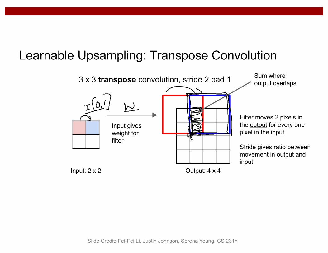
Learnable Upsampling: Transpose Convolution
3 x 3 transpose convolution, stride 2 pad 1
Input: 2 x 2 Output: 4 x 4
Slide Credit: Fei-Fei Li, Justin Johnson, Serena Yeung, CS 231n

Input: 2 x 2 Output: 4 x 4
Input gives weight for filter
Learnable Upsampling: Transpose Convolution
3 x 3 transpose convolution, stride 2 pad 1
Slide Credit: Fei-Fei Li, Justin Johnson, Serena Yeung, CS 231n
Input: 2 x 2 Output: 4 x 4
Input gives weight for filter
Sum where output overlaps
Learnable Upsampling: Transpose Convolution
3 x 3 transpose convolution, stride 2 pad 1
Filter moves 2 pixels in the output for every one pixel in the input
Stride gives ratio between movement in output and input
Slide Credit: Fei-Fei Li, Justin Johnson, Serena Yeung, CS 231n
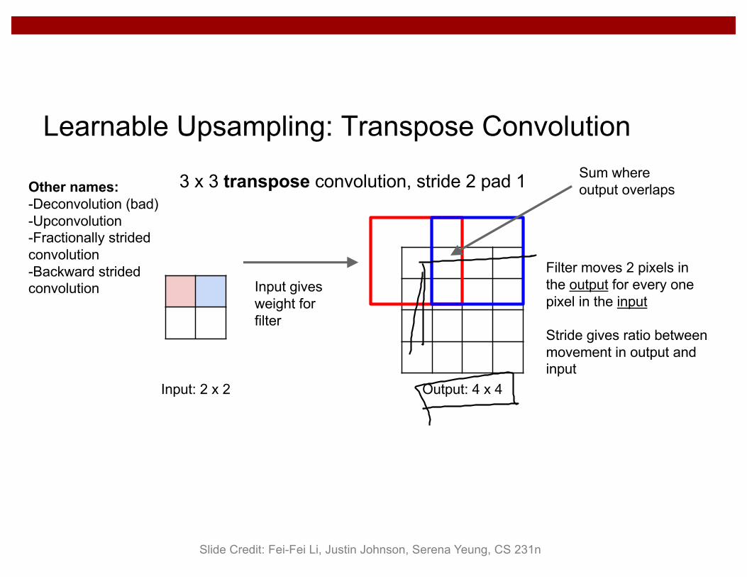
Input: 2 x 2 Output: 4 x 4
Input gives weight for filter
Sum where output overlaps
Learnable Upsampling: Transpose Convolution
3 x 3 transpose convolution, stride 2 pad 1
Filter moves 2 pixels in the output for every one pixel in the input
Stride gives ratio between movement in output and input
Other names:-Deconvolution (bad)-Upconvolution-Fractionally stridedconvolution-Backward stridedconvolution
Slide Credit: Fei-Fei Li, Justin Johnson, Serena Yeung, CS 231n

Transpose Convolution: 1D Example
a
b
x
y
z
ax
ay
az + bx
by
bz
Input FilterOutput
Output contains copies of the filter weighted by the input, summing at where at overlaps in the output
Need to crop one pixel from output to make output exactly 2x input
Slide Credit: Fei-Fei Li, Justin Johnson, Serena Yeung, CS 231n

Transposed Convolution• https://distill.pub/2016/deconv-checkerboard/
(C) Dhruv Batra 69