CROSS TABULATIONS / White

2004 World Cultures 14(2):179-193 A Student’s Guide to Statistics for Analysis of Cross Tabulations

Douglas R. White School of Social Sciences, 3151 Social Science Plaza, University of California, Irvine, CA 92697; drwhite@uci.edu Cross tabulations of qualitative data are a fundamental tool of empirical research. Their interpretation in terms of testing hypotheses requires a number of relatively simple concepts in statistical analysis that derive from probability theory. When strictly independent events having two characteristics that are independently defined are tabulated in a contingency table, the laws of probability can be used to model, from the marginal totals (rows, columns) of the table, what its cell values would be if the variables were statistically independent. The actual cell values of the frequency table can be used to measure the correlation between variables (with zero correlation corresponding to statistical independence), they can be compared to expected values under the null hypothesis of statistical independence, and they can be used to give a significance-test estimate of the probability that the departure of the observed correlation from zero (statistical independence) is simply a matter of chance. Further, when the sample of observations departs from strict independence because of observed interactions between them, the correlations between interacting neighbors measured on the same variables can be used to deflate effective sample size in obtaining accurate significance tests. 1. INTRODUCTION The goal here is to assist students in understanding the statistics they need in doing empirical research using cross tabulations of variables that are available for analysis observational samples, notably in the social sciences. Section 2, Core Ideas of Statistics for Hypothesis Testing in Empirical research, introduces the background in probability theory for the methods discussed in Statistical Analysis of Cross Tabulations (Section 3). This section, the core of this review, provides a minimal set of basic methods needed for the analysis of nominal and ordinal data. Abbreviated treatment of the problems of Controlling for Design Effects and Galton’s Problem of Autocorrelation (Section 40 and Inferential Statistics (Section 5) are followed by a Conclusion (Section 6) that summarize the relevance of basic statistics for empirical research on sample data. Some on-line calculators, references for articles on autocorrelation, and on-line statistical references are recommended for student use are provided in Section 7. Inferential statistics includes making predictions, determining relationships (e.g., using correlation coefficients), hypothesis testing with significance tests (e.g., both for the null hypothesis and for the similarity between two predicted outcomes), making inferences (e.g., generalizing from a sample statistic to population parameters). That will be the primary concern of this discussion. Descriptive statistics includes collecting, organizing, summarizing and presenting descriptive data. I will assume that the collection, data cleaning, and organization of data into variables has been done, and that the student has access to a database through a program such as SPSS (the Statistical Packages for the Social Sciences).

CROSS TABULATIONS / White

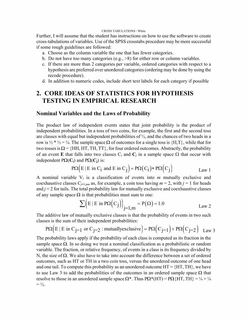
Further, I will assume that the student has instructions on how to use the software to create cross-tabulations of variables. Use of the SPSS crosstabs procedure may be more successful if some rough guidelines are followed:

a. Choose as the column variable the one that has fewer categories. b. Do not have too many categories (e.g., >8) for either row or column variables. c. If there are more than 2 categories per variable, ordered categories with respect to a

hypothesis are preferred over unordered categories (ordering may be done by using the recode procedure).

d. In addition to numeric codes, include short text labels for each category if possible 2. CORE IDEAS OF STATISTICS FOR HYPOTHESIS

TESTING IN EMPIRICAL RESEARCH Nominal Variables and the Laws of Probability The product law of independent events states that joint probability is the product of independent probabilities. In a toss of two coins, for example, the first and the second toss are classes with equal but independent probabilities of ½, and the chances of two heads in a row is ½ * ½ = ¼. The sample space Ω of outcomes for a single toss is H,T, while that for two tosses is Ω = HH, HT, TH, TT, for four ordered outcomes. Abstractly, the probability of an event E that falls into two classes Ci and Cj in a sample space Ω that occur with independent PΩ(Ci) and PΩ(Cj) is:

( ) ( ) ( )P E | E in C and E in C P C P Ci j iΩ = Ω j∗ Ω Law 1 A nominal variable Vi is a classification of events into m mutually exclusive and coexhaustive classes Cj=1,m, as, for example, a coin toss having m = 2, with j = 1 for heads and j = 2 for tails. The total probability law for mutually exclusive and coexhaustive classes of any sample space Ω is that probabilities must sum to one:

( )( ) ( )E | E in P C P 1.0j j 1,mΩ = Ω

=∑ = Law 2

The additive law of mutually exclusive classes is that the probability of events in two such classes is the sum of their independent probabilities:

( ) ( ) ( )P E | E in C or C : mutuallyexclusive P C P Cj=1 j=2 j=1 j=2Ω = Ω + Ω Law 3 The probability laws apply if the probability of each class is computed as its fraction in the sample space Ω. In so doing we treat a nominal classification as a probabilistic or random variable. The fraction, or relative frequency, of events in a class is its frequency divided by N, the size of Ω. We also have to take into account the difference between a set of ordered outcomes, such as HT or TH in a two coin toss, versus the unordered outcome of one head and one tail. To compute this probability as an unordered outcome HT = HT, TH, we have to use Law 3 to add the probabilities of the outcomes in an ordered sample space Ω that resolve to those in an unordered sample space Ω*. Thus PΩ*(HT) = PΩHT, TH = ¼ + ¼ = ½.

CROSS TABULATIONS / White

Unlike heads and tails in a coin toss, the probability of even or odd in roulette does not sum to one because casino profits derive from a sample space Ω with 37 outcomes, one of which is neither red, black nor even, odd (In the casino photo at http://www.roulette.sh/, the 37th slot is conveniently concealed). Here the probability PΩ (even) = PΩ(odd) =18/37 < ½ and by Law 3 PΩ (even or odd) = 18/37 + 18/37 = 36/37 < 1.0. Adding probabilities, Law 2 is satisfied by P(Ω) = PΩ (even or odd) or PΩ(neither even or odd) =36/37 + 1/37 = 1.0. Although the probability PΩ(odd) =18/37 < ½ and that of PΩ(red) =18/37 < ½, the probability of both red and odd is not the direct product of their probabilities on the space Ω of 37 outcomes. It is only the sample space Ω* of the 36 outcomes where red and odd are independent that PΩ*(red and odd) = ½ * ½ = ¼ = 8/36 by Law 3. For the space Ω of 37 outcomes, Law 2 applies so that PΩ (red and odd or outcome 37) = PΩ (red and odd) + PΩ(outcome 37) = 8/37 + 1/37 = 9/37. Hence PΩ (red and odd) = 8/37 < ¼. Probabilities in a coin toss would be identical to those in roulette if the chances of neither heads nor tails (i.e., balancing on the edge) were 1/37. Application of probability theory to empirical examples requires careful assessment of what event classes are independent and in what sample space. Law 3, for example, is especially sensitive to nonindependence of units sampled where there are clustered similarities in the sample space Ω. These problems are taken up in section 4, Controlling for Design Effects and Galton’s Problem of Autocorrelation. As Kruskal (1988:929) warned: “do not multiply lightly” (meaning: take care in evaluating the assumption of independence in Law 3, and make appropriate adjustments). Dow (1993), for example, has examined the adjustments required for the analysis of cross-tabulations for samples with clustered similarities. Ordinal, Interval and Ratio Scale Variables An ordinal variable Vi is a classification of events into mutually exclusive classes that are rank-ordered by some criterion. An interval variable Vi is a classification of events by a numeric measurement in which one unit on the scale represents the same magnitude on the trait or characteristic being measured across the whole range of the scale. Operations of addition and multiplication by constants do not change the interval property of the scale. Such transformations are made, for example, in converting Centigrade to Fahrenheit temperature: multiply °C by 1.6 and add 32 to get °F. Twenty degrees is not twice as hot, however, than ten degrees. That property is the characteristic of a ratio scale such as the Kelvin scale of temperature in which 0°K is absolute zero, and 20°K is twice the heat (measured by motion of molecules) as 20°K.

CROSS TABULATIONS / White

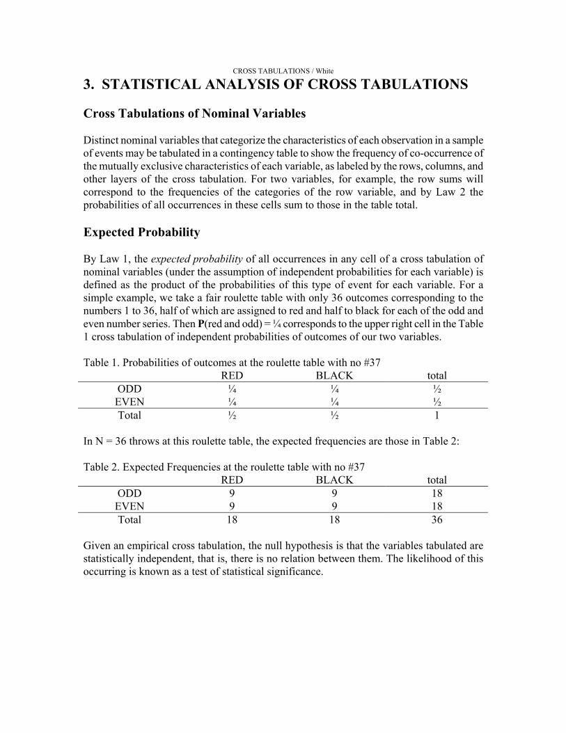
3. STATISTICAL ANALYSIS OF CROSS TABULATIONS Cross Tabulations of Nominal Variables Distinct nominal variables that categorize the characteristics of each observation in a sample of events may be tabulated in a contingency table to show the frequency of co-occurrence of the mutually exclusive characteristics of each variable, as labeled by the rows, columns, and other layers of the cross tabulation. For two variables, for example, the row sums will correspond to the frequencies of the categories of the row variable, and by Law 2 the probabilities of all occurrences in these cells sum to those in the table total. Expected Probability By Law 1, the expected probability of all occurrences in any cell of a cross tabulation of nominal variables (under the assumption of independent probabilities for each variable) is defined as the product of the probabilities of this type of event for each variable. For a simple example, we take a fair roulette table with only 36 outcomes corresponding to the numbers 1 to 36, half of which are assigned to red and half to black for each of the odd and even number series. Then P(red and odd) = ¼ corresponds to the upper right cell in the Table 1 cross tabulation of independent probabilities of outcomes of our two variables. Table 1. Probabilities of outcomes at the roulette table with no #37

RED BLACK total ODD ¼ ¼ ½ EVEN ¼ ¼ ½ Total ½ ½ 1

In N = 36 throws at this roulette table, the expected frequencies are those in Table 2: Table 2. Expected Frequencies at the roulette table with no #37

RED BLACK total ODD 9 9 18 EVEN 9 9 18 Total 18 18 36

Given an empirical cross tabulation, the null hypothesis is that the variables tabulated are statistically independent, that is, there is no relation between them. The likelihood of this occurring is known as a test of statistical significance.

CROSS TABULATIONS / White

Expected Frequencies under the Null Hypothesis Say, for example, an investigator surveyed 36 people whether they preferred the color red or the color blue. There were different numbers of males and females in the sample and the outcome of the survey are given in Table 3: Table 3. Survey Results

RED BLUE total FEMALE 4 15 19

MALE 7 10 17 Total 11 25 36

Overall, blue was preferred to red. Is there a difference between the preferences of males and females? The expected frequencies Hr,c under the null hypothesis of no difference can be computed as follows by the formula Hr,c = N* Pr * Pc where the probabilities of row and column characteristics Pr and Pc are estimated from the relative proportions of the row and column sums, Fr and Fc in the total sample. Hence Pr = Fr /N for rowr=1,2 and Pc = Fc /N for columnc=1,2. Thus Pr=1(red) = Fr=1(red) / N = 11/36 =0.305555, as in Table 4. Expected frequencies are given in Table 5. Table 4. Survey Results with row and column probabilities calculated from frequencies

RED BLUE Total Fr Pr FEMALE 4 15 19 0.527777

MALE 7 10 17 0.472222 Total Fc 11 25 36

Pc (red, blue) 0.305555 0.694444 Table 5. Expected Frequencies from independent row and column probabilities

RED BLUE Total Fr Pr FEMALE 5.805 13.195 19 0.527777

MALE 5.195 11.805 17 0.472222 Total Fc 11 25 36

Pc (red, blue) 0.305555 0.694444 Chi-square Statistic for Measuring Departure from Null Hypothesis One way to calculate the degree of difference between males and females in this survey is to compute the Chi-square statistic. Because larger differences between expected and actual frequencies are more important than smaller ones, the differences are computed and then squared in Tables 6 and 7.

CROSS TABULATIONS / White

Table 6. Difference between Survey Results and Expected Frequencies

Difference: RED BLUE Squared Difference: RED BLUE

FEMALE +1.805 -1.805 3.26 3.26 MALE -1.805 +1.805 3.26 3.26

Table 7. Squared Differences Divided by Expected Frequencies

RED BLUE FEMALE 3.26 / 5.805 = 0.562 3.26 / 13.195 = 0.247

MALE 3.26 / 5.195 = 0.623 3.26 / 11.805 = 0.276 To get a total Chi-square statistic for a table, the Chi-square values χ2

r,c for individual r,c cells of the table are summed, so that χ2 = Σχ2

r,c. In the case of Table 7, χ2 = 1.71. Phi-square Correlation Coefficient Φ2 The correlation coefficient phi(Φ) is computed as Φ2 = χ2 / N, which in the case of Table3-7 is Φ2 = 1.71 / 36 = 0.0475. Phi square (Φ2) is a measure of the variance accounted for in predicting one variable from the other. Is this a significant correlation? It is obviously quite low since it is close to zero, and less than 5% of the variance in responses is predicted from differences in gender. A crucial condition for the accuracy of Phi square and Chi square in contingency table analysis is that expected frequencies under the hypothesis of independence must exceed five for each cell in the table. When this assumption is violated, chi square values do not qualify for theoretical interpretation (the inaccuracy comes from dividing by expected values), and the phi square may even exceed 1.0, which is automatically disqualified by the definition of a correlation coefficient. To satisfy this condition, the contingency table must not have row or column sums that are too small, and in general, with lower sample sizes, only those crosstabs with relatively few categories will be appropriate for these statistical tests. Fisher exact tests, however, are appropriate for uneven marginals and small sample sizes, and calculators can be found for not only 2x2 tables, but for tables having up to 2x5 cells (see http://home.clara.next.sisa). Are males and females different? Consider the value that Φ2 would take in the case of prefect correlation of Φ2 = Φ = 1.0 that would have occurred if all males said red and all females said blue. Here is we compute Chi square we get χ2 = 36.0 and Φ2 = 36/36 = 1.0, as expected. This shows that Phi square conforms to the rule that the maximum value of a correlation coefficient is 1.0.

CROSS TABULATIONS / White

Phi Correlation Coefficient Φ: Assigning a Positive or Negative Sign What if we had a negative correlation? Then we would expect a correlation coefficient to take the value of –1.0. Since Φ2 as calculated from χ2 is always positive, when we compute

2Φ = Φ we have a choice of assigning a positive or negative sign to Φ since square roots of positive numbers may be positive or negative. In Table 8 the negative correlation is between female and red, male and blue, but we can also say that the positive correlation is between male and red, female and blue; i.e., depending on how we view the table. Table 8. A Hypothetical Perfect Correlation, with Φ2 = 1.0 for the Survey Sample

RED BLUE Total Fr Pr FEMALE 0 19 19 0.527777

MALE 17 0 17 0.472222 Total Fc 17 19 36

Pc (red, blue) 0.47222 0.527777 Evaluating Cross Tabulations of Nominal Variables Care must be taken in giving a sign to Φ because Φ2 in general is a measure of predictability between nominal variables. If our respondents fell into three sets, as in Table 9, we might have difficulty assigning a sign to Φ because, while the relationship between age and color preference is perfectly predictive (Φ2 = 1.0), there is no sense of a positive or negative correlation with age in Table 9 since the relationship to color preference is curvilinear. Table 9. A Hypothetical Perfect Correlation, with Φ2 = 1.0 for the Survey Sample

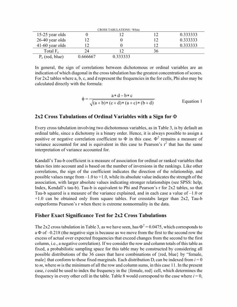
RED BLUE Total Fr Pr 15-25 year olds 0 12 12 0.333333 26-40 year olds 12 0 12 0.333333 41-60 year olds 0 12 12 0.333333

Total Fc 12 24 36 Pc (red, blue) 0.333333 0.666667

Cross Tabulations of Ordinal Variables If, however, the sample of responses had looked like that of Table 10, we could assign the Φ coefficient a negative sign, Φ = -1.0 between age and preference for blue. Equivalently, we could say that Φ = 1.0 between age and preference for red. The three categories of age in this table constitute an ordinal variable because they are rank ordered by the criterion of age. In this context, if the proportions of red :: blue in successive rows and those of young :: middle age :: elderly in successive columns are monotonically increasing or decreasing in every case, Phi can be given a sign and interpreted as an ordinal correlation. Table 10. A Hypothetical Perfect Correlation, with Φ2 = 1.0 for a Different Survey Sample

RED BLUE Total Fr Pr

CROSS TABULATIONS / White

15-25 year olds 0 12 12 0.333333 26-40 year olds 12 0 12 0.333333 41-60 year olds 12 0 12 0.333333

Total Fc 24 12 36 Pc (red, blue) 0.666667 0.333333

In general, the sign of correlations between dichotomous or ordinal variables are an indication of which diagonal in the cross tabulation has the greatest concentration of scores. For 2x2 tables where a, b, c, and d represent the frequencies in the for cells, Phi also may be calculated directly with the formula:

a d b c

(a b) (c d) (a c) (b d)∗ − ∗

φ =+ ∗ + ∗ + ∗ + Equation 1

2x2 Cross Tabulations of Ordinal Variables with a Sign for Φ Every cross tabulation involving two dichotomous variables, as in Table 3, is by default an ordinal table, since a dichotomy is a binary order. Hence, it is always possible to assign a positive or negative correlation coefficient to Φ in this case. Φ2 remains a measure of variance accounted for and is equivalent in this case to Pearson’s r2 that has the same interpretation of variance accounted for. Kandall’s Tau-b coefficient is a measure of association for ordinal or ranked variables that takes ties into account and is based on the number of inversions in the rankings. Like other correlations, the sign of the coefficient indicates the direction of the relationship, and possible values range from –1.0 to +1.0, while its absolute value indicates the strength of the association, with larger absolute values indicating stronger relationships (see SPSS: help, Index, Kendall’s tau-b). Tau-b is equivalent to Phi and Pearson’s r for 2x2 tables, so that Tau-b squared is a measure of the variance explained, and in each case a value of –1.0 or +1.0 can be obtained only from square tables. For crosstabs larger than 2x2, Tau-b outperforms Pearson’s r when there is extreme nonnormality in the data. Fisher Exact Significance Test for 2x2 Cross Tabulations The 2x2 cross tabulation in Table 3, as we have seen, has Φ2 = 0.0475, which corresponds to a Φ of –0.218 (the negative sign is because as we move from the first to the second row the excess of actual over expected frequencies that exceed changes from the second to the first column, i.e., a negative correlation). If we consider the row and column totals of this table as fixed, a probabilistic sampling space for this table may be constructed by considering all possible distributions of the 36 cases that have combinations of red, blue by “female, male that conform to these fixed marginals. Each distribution Di can be indexed from i = 0 to m, where m is the minimum of all the row and column sums, in this case 11. In the present case, i could be used to index the frequency in the female, red cell, which determines the frequency in every other cell in the table. Table 8 would correspond to the case where i = 0,

CROSS TABULATIONS / White

and to the last table in Table 11 (next page), which shows only those tables indexed to i = 0,3, that represent a more extreme distribution than that in Table 3. Given this indexing system for the sampling space from which the actual distribution may be drawn with fixed independent probabilities of the variables tabulated, the probability of each specific distribution Di for i = 0 to m can be computed exactly by a permutational formula called the Fisher Exact test. Here the product of successive integers from 1 to N (N! or N factorial) defines the size of the total sample space of all possible cell values of 2X2 tables with N = 36. Subsamples that meet the four marginal constraints for cells Frc!F~rc!Fr~c!F~r~c! and marginals Fr.!F~r.!F.c!F.~c! are defined by the expression (M choose m) that refers to the number of ways there are to draw m elements in a cell given the marginal total of size M. Then the probability Prc of the value in a cell with Frc elements is:

( )( )( )( )( )

P F F F F F F F F / NF !F !F F / N!F !F !F !F !

= choose choose choose choose rc r. rc ~r. ~rc .c r~c .~c ~r~c = r. ~r. .c .~c rc ~rc r~c ~r~c

!

Equation 2 Table 11. Possible tables from the probabilistic sampling space of Table 3, but which are more extreme (higher negative correlation) than Table 3.

i = 3 RED BLUE total FEMALE 3 16 19

MALE 8 9 17 Total 11 25 36

i = 2 RED BLUE total

FEMALE 2 17 19 MALE 9 8 17 Total 11 25 36

i = 1 RED BLUE total

FEMALE 1 18 19 MALE 10 7 17 Total 11 25 36

i = 0 RED BLUE total

FEMALE 0 19 19 MALE 11 6 17 Total 11 25 36

CROSS TABULATIONS / White

Starting with the observed table, Table 3, and continuing through the tables with more extreme departure from randomness but the same marginal totals (those in Table 11), P values for five distinctive tables are computed, indexed on the red, female cell frequency i = 0 to m:

Prc = 19!17!11!25! / 36!4!15!7!10! = 0.12547 [Table 3] = 19!17!11!25! / 36!3!16!8!9! = 0.03921 [Table 11.1] = 19!17!11!25! / 36!2!17!9!8! = 0.00692 [Table 11.2] = 19!17!11!25! / 36!1!18!10!7! = 0.00062 [Table 11.3] = 19!17!11!25! / 36!0!19!11!6! = 0.00002 [Table 11.4] These sum to: 0.17224

Thus p =0.17224 is the exact probability for the occurrence of Table 3 or more extreme distributions with the same marginals. Degrees of Freedom The degrees of freedom, df, of a crosstab are the number of cells that must be filled before all the cell values are determined by the marginal (row, column) totals. In a 2x2 table there is one degree of freedom. If R is the number of rows and C is the number of columns:

( ) ( )df R 1 C 1= − ∗ − Equation 3 Significance Tests: The Chi-square Approximation Significance in a statistical sense is the probability that the observed χ2 and Φ2 values would occur, given the N of the table, if the probabilities of the two nominal variables were independent. For a 2x2 cross tabulation, Fishers Exact test is the most direct, accurate and powerful way to calculate this. Significance tests indicate whether it is worthwhile to interpret a contingency table. A significant result means that the cells of a contingency table should be interpreted. A non-significant test means that no effects were discovered and chance could explain the observed differences in the cells. In this case, an interpretation of the cell frequencies is not useful. Standard cut-offs considered significant are p ≤ 0.05 and p ≤ 0.01, which mean there are respectively fewer than five or one chances in 100 that the observed correlation is due to chance. Chi-square can be used to give a conservative approximation of the level of significance as calculated by the Fisher Exact Test, or, in the more general case of tables with more than two rows and columns, a conservative approximation of the level of significance. Since the shape of the theoretical distribution relating Chi-square values to probabilities changes from a monotonically decreasing function at one degree of freedom towards a more normal (or Gaussian) curve as degrees of freedom increase, there are lookup tables and calculators to make the conversion. The calculator at http://www.stat.sc.edu/webstat/ gives the corresponding probability of p =0.19 for the Chi-square value in Table 3 (df = 1), which is close to, but less sensitive than, the exact probability (p = 0.17) from Fisher’s Exact test.

CROSS TABULATIONS / White

4. CONTROLLING FOR DESIGN EFFECTS AND GALTON’S PROBLEM OF AUTOCORRELATION

Chi-square and Fisher Exact Tests err in rejecting the null hypothesis too often when data have been generated using a sampling scheme that does not ensure complete independence of sampling units (see Dow, Burton and White 1982; Dow et al. 1984; Dow 1993; Ferguson, Genest and Hallin 2000). The units sampled are not independent, for example, when subsets of given numbers of related observations in a sample – related by spatial adjacency or networks of interaction – are more similar than comparable subsets drawn at random. Analytical, empirical and simulation studies of this problem show that the effectively independent size of a sample is not the original N, but typically varies between N and N/2 depending on the degree of nonindependence, with the design effect (DE) of nonindependence varying accordingly from DE = 1 for a simple random sample of independent cases to not much more than DE = 2 (the fractional divisor) for a sample with highly nonindependent clusters. My current rule of thumb for adjusting the significance of a Φ2

12 Phi-square correlation between two variables is to let DE = 1 + Φ211 + Φ2

22 +Φ11 Φ22, where Φ2

11 and Φ222 are the Φ2 variance autocorrelations between neighbors for each of the

variables (1 and 2), and Φ11 Φ22 is their product. Some samples, however, have much higher design effects. 5. PROBLEMS OF INFERENCE From Sample Statistics to Population Parameters If observations are sampled randomly from a population, or one or more observations are sampled randomly from local clusters of cases known to interact, inferences can be drawn from correlations in the sample as to correlations in the population. Typically, sample estimates of correlations are unbiased estimates of population correlations, regardless of the degree of nonindependence of cases, which usually requires deflation of effective sample sizes in computing significance levels and thus lowering the rejection rate of the null hypotheses. In exceptional cases, however, Φ11 and Φ22 autocorrelations and interactions among sample units bias the estimation of population correlations and the estimation of correlations based on samples of strictly independent cases in the population, which are slightly different problems of inferential statistics. In any case, potential sources of bias – such as observer bias, measurement bias, selection bias, mortality bias, and possible autocorrelation bias (like the effects of negative Φ11 and positive Φ22 autocorrelations) – require examination in their own right as safeguards to valid inferences from contingency tables. Naive Cross Tabulation Tests and the Problem of Specification Statistically significant correlations, even with corrections for autocorrelation, are not indices of causal relationships among variables. The model specification problem is one of choosing the best fit among alternative models, which implies that all variables relevant to

CROSS TABULATIONS / White

the problem have been considered. It is not really possible to tell when a model is correctly specified, except to say that with a sufficient number of observations, a correctly specified model should give the same results when other unspecified variables are entered into the prediction. A clue to misspecification in predicting outcome variables from a set of independent variables, for example in multiple regression models where variables and error terms in fitting models are continuous, is that the error terms are not randomly distributed. Software programs for statistical analysis with cross tabulation allow multiple layers to be added to cross tabulations (SPSS, for example, has a place for additional layer variables beyond row and column using the ‘next’ command to add subsequent layers). With cross tabulation, the addition of control variables makes it possible to study higher order interactions among three or more variables (given a sufficient number of observations) and to test for misspecification by adding a control variable to determine whether lower order interactions are altered by the presence or absence of the control. Misspecification occurs when the control variable makes a significant difference, which implies that the lower order relationship among variables is unstable. In this context, it is meaningful to discuss the specification problem with respect to two types of error in testing the null hypothesis:

Type I error is rejecting the null hypothesis when it is true Type II error is accepting the null hypothesis when it is false.

The correlation between postmarital residence of husband and wife and female contribution to subsistence labor (hunting, gathering, fishing, animal husbandry and agriculture), for example, is so close to zero even for large samples of societies (e.g., N = 1280) as to be non-significant. Korotayev (2000) ran a multiple regression analysis of General Non-Sororal Polygyny and Female Contribution to Subsistence as predictors of Marital Residence that showed a negative regression coefficient for the former independent variable (beta = -0.34, p < 0.001) and a positive coefficient for the latter (beta = +0.10, p = 0.02) in the same sample with N = 1280 (including missing cases) and with nearly identical results in a smaller sample (N = 186) with lesser clustering of similar cases. Thus, the zero correlation relationship between residence and division of labor is misspecified without inclusion of whether non-sororal polygyny is present (in which case the correlation is zero) or absent, in which case the correlation between matridominant labor and matrilocality is positive (and similarly for patridominant labor and patrilocality). For the larger sample analyzed by Korotayev, a recoding and cross tabulation of variables similar to his (Table 12, next page) shows that when non-sororal polygyny is absent Φ = 0.165 (p = 0.020) and tau-b = 0.11 (p = 0.012), supporting his result. If the middle category of residence is removed, where the bride does not move to live with the husband’s group nor the reverse, then Φ = 0.159 (p = 0.011) and tau-b = 0.135 (p = 0.009), a somewhat stronger result. However, when a further layer is added to control for region, only the indigenous societies of North America show a significant positive tau-b (0.153, p = 0.042). Hence, the three-way interaction between these variables may still be underspecified. That is, other, as yet unspecified, variables may also intervene in the relationship between division of labor and residential pattern.

CROSS TABULATIONS / White

6. CONCLUSION When strictly independent events having two characteristics that are independently defined are tabulated in a contingency table, the laws of probability can be used to model, from the marginal totals (rows, columns) of the table, what its cell values would be if the variables were statistically independent. The actual cell values of the frequency table can be used to measure the correlation between the variables (with a correlation of zero corresponding to statistical independence), they can be compared to expected values under the null hypothesis of statistical independence, and they can be used to give a significance-test estimate of the probability that the departure of the observed correlation from zero (statistical independence) is simply a matter of chance. Further, when the sample of observations departs from strict independence because of observed interactions between them, the correlations between interacting neighbors measured on the same variables can be used to deflate effective sample size to obtain accurate significance tests. Table 12. Influence of a Third Variable on Two-Way Cross Tabulation Results

Polygyny Division of Labor Residence Rule Total

Male Dominant

104 64.6%

31 19.3%

26 16.1%

161 100.0%

Balanced 102 66.7%

21 13.7%

30 19.6%

153 100.0%

Monogamy or sororal polygyny Female

Dominant 58

49.6% 25

21.4% 34

29.1% 117

100.0%

TOTAL 264 61.3%

77 17.9%

90 20.9%

431 100.0%

Male Dominant

37 88.1%

2 4.8%

3 7.1%

42 100.0%

Balanced 56 86.2%

4 6.2%

5 7.7%

65 100.0%

Non-Sororal polygyny

Female Dominant

75 88.2%

6 7.1%

4 4.7%

85 100.0%

TOTAL 168 87.5%

12 6.3%

12 6.3%

192 100.0%

7. REFERENCES Calculators SISA: Simple Interactive Statistical Analysis (multiple calculators)

http://home.clara.net/sisa (see Two by Two Table; Fisher Exact; Ordinal Tests; Fisher 2*5; Ordinal 2*5 http://home.clara.net/sisa/ord2hlp.htm; Correlations; Significance Testing; Power)

CROSS TABULATIONS / White

West, R. Webster, and R. Todd Ogden. 2000. WebStat 2.0 (calculator) http://www.stat.sc.edu/webstat/ --click refresh to start if page does not open. Click “fire up.” Click Contingency Table #rows #cols. Click individual cells to enter values to generate Chi square and p values for significance (and Phi square).

On-Line References Garson, G. David. Instructor. Fisher Exact Test of Significance. Quantitative Research in Public Administration.

http://www2.chass.ncsu.edu/garson/pa765/fisher.html Korotayev, Andrey

2001 An Apologia of George Peter Murdock. Division of Labor by Gender and Postmarital Residence in Cross-Cultural Perspective: A Reconsideration. World Cultures 12(2): 179-203. http://www.worldcultures.org/~eclectic/drwhite/worldcul/12-2korotayev.pdf

PinkMonkey.com. Statistics Study Guide. http://www.pinkmonkey.com/studyguides/subjects/stats/contents.asp

Stockburger, David W. Author. Chi square and Tests of Contingency Tables. Introductory Statistics: Concepts, Models, and Applications. http://www.psychstat.smsu.edu/introbook/sbk28m.htm

Symynet Educational Statistics Software. Tutorials on Statistics Topics http://www.symynet.com/educational_software/sitemap.htm

Trochim, William M. K. Selecting Statistics: Glossary. Cornell University http://trochim.human.cornell.edu/selstat/glossary.htm

Articles on Autocorrelation Dow, Malcolm

1993 Saving the Theory: On Chi-Square Tests with Cross-Cultural Survey Data. Cross-Cultural Research 27:247-276.

Dow, Malcolm, Michael L. Burton, and Douglas R. White 1982 Network Autocorrelation: A Simulation Study of a Foundational Problem in Regression and Survey Research. Social Networks 4:169-200.

CROSS TABULATIONS / White

Dow, Malcolm, Michael L. Burton, Douglas R. White, and Karl P. Reitz 1984 Galton’s Problem as Network Autocorrelation. American Ethnologist 11:754-770.

Ferguson, Thomas S., Christian Genest, and Marc Hallin 2000 Kendall’s tau for Autocorrelation. http://citeseer.nj.nec.com/241781.html

Kruskal, William 1988 Miracles and Statistics: The Causal Assumption of Independence. Journal of the American Statistical Association 83:929-940.

Reitz, Karl P., and Malcolm M. Dow 1989 Network Interdependency of Sample Units in Contingency Tables. Journal of Mathematical Sociology 14:85-96.

Statistics Text Kachigan, Sam

1982 Statistical Analysis. New York: Radius Press. Acknowledgement My thanks to Andrey Korotayev and Patrick Gray for helpful commentary on earlier drafts.

CD DATA DISK / Divale

2003 World Cultures 14(2):194

World Cultures CD Data Disk The CD with this issue of World Cultures contains the following files in the different directories. In addition, with this issue of WC we begin a new feature where we include the Program and Abstracts of the Annual Meetings of the Society for Cross-Cultural Research. \WORLD CULTURES VOL 14#2 WC14#2.DOC Issue in Word 2000 and PDF format

There are also two subdirectories in \WORLD CULTURES VOL 14#2: \DOW This subdirectory contains the sccs.Rdata file discussed in Dow’s article. \DEMEO This subdirectory contains *.tif files for the figures in DeMeo’s article.

In addition, there are the following directories on the CD: \Corrected Maptab Data Files This subdirectory contains the Maptab program plus the Maptab data files for the SCCS. \Ethnographic Atlas Revised by World Cultures This subdirectory contains the complete revised Ethnographic Atlas of 112 variables for 1267 cultures. Data file is in SPSS *.sav format. \Std Cross-Cultural Sample Manuals This subdirectory contains the codebooks for the 2,000 variables in the SCCS and the ethnographic references for the 186 societies in the sample. \Std Cross-Cultural Sample SPSS Data Files This subdirectory contains all the variables (approx. 2,000) published for the Standard Cross-Cultural Sample with codebooks (186 societies). Data file is in SPSS *.sav format. \Western North American Indians Data Set This subdirectory contains all the variables (approx. 441) for the 172 North American Indian societies compiled by Dr. Harold Driver. Data file is in SPSS *.sav format. \World Cultures Volumes 01#1 – 14#1 This subdirectory contains all previous issues of World Cultures (1#1 to 14#1). \Society for Cross-Cultural Research

CD DATA DISK / Divale

This subdirectory contains the Annual Program and Abstracts of the meetings of the Society for Cross-Cultural Research. At present we have the programs and abstracts for the SCCR meetings in 1989, 1998, 2001, 2002, and 2004. These files are in PDF format. Future Codes: The next issue of World Cultures (vol. 15#1) will contains several new codes for the Standard Cross-Cultural Sample. Codes will be for Homosexuality and Transvestites, Female Status, Status of the Aged, and Individualism-Collectivism.

William Divale

Social Evolution and History

The new international Journal ‘Social Evolution and History’ (SEH), has been founded to meet he needs of those seeking an understanding of how human societies developed in the past and continue to develop in the present. While dozens of journals dealing with organic evolution have the words ‘Biological Evolution’ in their titles, hardly a journal exists in the whole world which includes ‘Social Evolution’ in its title. This alone seems like a compelling reason to establish a new journal, devoted in title and contents, to social evolution specifically. The editors believe that Social Evolution and History is the appropriate title for this new journal. It suggests not only the journal’s contents, but also its theoretical perspective. The journal will focus on the achievements of different sciences, and examine social transformations, not as a stream of disjointed events, but as an intelligible and determinate process, whether involving a shorter or a longer time span. The journal’s aim is to contribute to the integration of such fields of knowledge as anthropology, history, sociology, and the philosophy and theory of history. Such integration has been lacking until now, though its necessity has long been felt acutely felt by the academic community. The journal Social Evolution and History is devoted to the study of many aspects of the evolutionary changes that have occurred over the long course of human history. We expect to publish theoretical, analytical, and synthetic articles. In its concern with the theoretical dimensions of human history, SEH will highlight crucial moments and components of history, as well as the various evolutionary pathways traveled by the world's societies, from simple villages to civilizations. One of foci of the Journal will be on the cultural activities of human beings, encompassing all spheres of everyday life. It will reflect the processes and simultaneities of cultural change that have occurred on both the microhistorical and macrohistorical levels. The Journal is published in English twice a year in March and September. Two parts form a volume.

Invitation to Subscription

If you would like to subscribe to Social Evolution & History, please contact one of the authorized distributors (see below). The prices suggested by the Journal Publisher are as follows: regular subscription rate for institutions is $50.00 per year, single issue rate $33.00. Individuals may subscribe at a one-year rate of $25.00, single-issue $17.00. Special subscription rates are available to students: $16.00, single-issue $10.00. However, please note that the Journal distributors naturally have the right to establish subscription rates of their own, and their prices may differ from one distributor to another.

The Social Evolution & History distributors: 1. East View Publications Inc. Address in the USA: 3020 Harbor Lane North, Minneapolis, Minnesota 55447 Tel.; +(763) 550-0961, Fax +(763) 559-2931 E-mail: eastview@eastview.com, periodicals@eastview.com Address in Russia: 6/3 Azovskaja Ulitsa, Moscow 113149 Tel.: +7(095) 318-0937, 777-6557 Fax: +7(095) 318-0881, E-mail: sales@mosinfo.ru There you can find hardcopy and electronic catalogues. The electronic catalogue is also available from http://www.eastview.com. (To find our Journal on the site and get all the necessary information you need only to type its name [Social Evolution & History] in the “Product Search” window). Note that by the moment the site indicates erroneously that the Journal is published in Russian, whereas in fact it is published in English. This mistake will be corrected soon. For all other permissions, requests or inquiries, please contact East View Publications Inc. directly. 2. JSC “MK-Periodica” You can subscribe through one of the partners of “MK-Periodica” in your country or through “MK-Periodica” directly. E-mail: info@periodicals.ru Address: 39 Gilyarovskogo Ulitsa, Moscow 129110, Russia. Tel.: +7(095) 281-91-37, 281-97-63; fax +7(095) 281-37-98. There you can find hardcopy and electronic catalogues. For all other permissions, requests or inquiries, please contact “MK-Periodica” directly. 3. “Nauka-Export” Company Address: 90 Profsouznaja Ulitsa, Moscow 117997, Russia Fax: +7(095) 334-74-79, 334-71-40. E-mail: nauka@naukae.msk.ru There you can find a hardcopy catalogue “Periodicals of Russia” “Nauka-Export” Company can send information about our journal by E-mail, fax, or by post for your request. For all other permissions, requests or inquiries, please contact “Nauka-Export” Company directly. 4. "Teza" Publishers Address : 14 Dobrolyubova Prospekt, Office 358, St. Petersburg 197198, Russia Tel/ fax: 7(812)238-95-94; 233-59-16. E-mail: bi@thesa.ru http://www.thesa-key.com You can subscribe to our Journal both through this site, or contacting this Publishing House by ordinary, or electronic mail. The payment can be made by check, or credit card. The relevant information is available at the above mentioned site. For all permissions, requests or inquiries, please contact: “Uchitel” Pulishing House E-mails: uchitel@avtlg.ru, ph_uchitel@vistcom.ru, lgrinin@vistcom.ru

Tel.:+7(8442)46-85-45, Fax +7(8442) 46-85-53. Address: 82-53, Bystrova Ulitsa, Volgograd 400067, Russia Your letters and calls are always welcomed!

You can order a free sample copy by mailing your request to: “Uchitel” Publishing House 82-53 Bystrova Ulitsa Volgograd 400067 Russia