Chapter 6 Reading Cross-Tabs

The statistical analyses of many cross tabulations would be normally able to extract a very small fraction of useful information from them. That is why one should be trained not only to get and to analyze a few numbers in conjunction with cross tabulations (i.e. correlation coefficients and significance measures), but the cross tabulations themselves. Let us take, for example, the cross tabulation between population density and political centralization (see Table 2.1 above). Assuming the causal link between the population density and political centralization the table could be read as follows:

"The state is entirely unlikely to appear in cultures with an extremely low population density (less than 1 person per 5 sq. miles). The overwhelming majority of cultures with such a low population density are organized politically in independent communities, the only plausible (but in no way frequent) alternative of political organization for such cultures appears to be simple chiefdom; even complex chiefdoms do not seem to be really likely to develop with such a low population density. The growth of population density over 1 person per 5 square miles (but still less than 1 person per 1 square mile) does not seem to tend to lead to any significant increase in political centralization. The situation changes significantly when the population density grows over 1 person per sq. mile (even before it reaches the level of 6 persons per sq. mile). The proportion of cultures organized in independent communities drops below 50%. Proportion of chiefdoms rises more than twice (whereas one third of the chiefdoms in this range are complex). Even states turn out to be able to get formed within this range of population density, though the probability of this is in no way high. The situation changes significantly once more when the population density grows over 6 persons per sq. mile (even before it reaches the level of 26 persons per sq. mile). The proportion of cultures organized in independent communities further drops almost twice. The proportion of cultures organized in states grows more than twice. Even large states / empires turn out to be able to get formed within this range of population density, though the probability of this is in no way high. On the other hand, the growth of population density over 26 persons per square mile (but still less than 101 persons per 1 square mile) does not seem to tend to lead to any significant increase in political centralization.

Reading Cross-Tabs

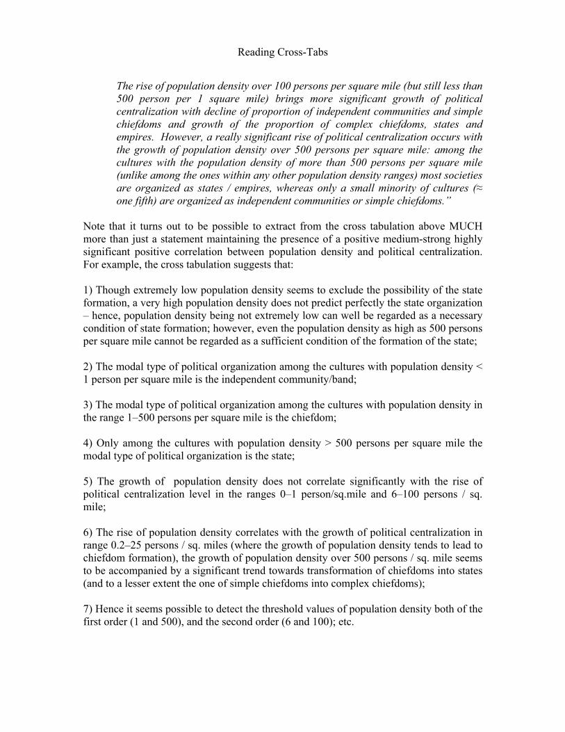
The rise of population density over 100 persons per square mile (but still less than 500 person per 1 square mile) brings more significant growth of political centralization with decline of proportion of independent communities and simple chiefdoms and growth of the proportion of complex chiefdoms, states and empires. However, a really significant rise of political centralization occurs with the growth of population density over 500 persons per square mile: among the cultures with the population density of more than 500 persons per square mile (unlike among the ones within any other population density ranges) most societies are organized as states / empires, whereas only a small minority of cultures (≈ one fifth) are organized as independent communities or simple chiefdoms.”

Note that it turns out to be possible to extract from the cross tabulation above MUCH more than just a statement maintaining the presence of a positive medium-strong highly significant positive correlation between population density and political centralization. For example, the cross tabulation suggests that: 1) Though extremely low population density seems to exclude the possibility of the state formation, a very high population density does not predict perfectly the state organization – hence, population density being not extremely low can well be regarded as a necessary condition of state formation; however, even the population density as high as 500 persons per square mile cannot be regarded as a sufficient condition of the formation of the state; 2) The modal type of political organization among the cultures with population density < 1 person per square mile is the independent community/band; 3) The modal type of political organization among the cultures with population density in the range 1–500 persons per square mile is the chiefdom; 4) Only among the cultures with population density > 500 persons per square mile the modal type of political organization is the state; 5) The growth of population density does not correlate significantly with the rise of political centralization level in the ranges 0–1 person/sq.mile and 6–100 persons / sq. mile; 6) The rise of population density correlates with the growth of political centralization in range 0.2–25 persons / sq. miles (where the growth of population density tends to lead to chiefdom formation), the growth of population density over 500 persons / sq. mile seems to be accompanied by a significant trend towards transformation of chiefdoms into states (and to a lesser extent the one of simple chiefdoms into complex chiefdoms); 7) Hence it seems possible to detect the threshold values of population density both of the first order (1 and 500), and the second order (6 and 100); etc.

Chapter 6

3

Of course, some of the statements above can be further tested statistically ("There is no significant correlation between population density and political centralization in the range 6–100 persons per square mile,” or "There is a significant correlation between population density and political centralization in the range 0.2–6 persons per square mile"), i.e., further meaningful questions could be posed. However, in order that such questions could be asked one should first just "read the table.” So. How to? HOW TO READ CROSS-TABS? The general rules here could be specified roughly in the following way: FIRST, YOU SHOULD DETERMINE WHICH WAY THE CROSS-TAB MUST BE READ – "BY COLUMNS,” OR "BY ROWS.” The general rule could be formulated here in the following way: 1. RULE 1: If the independent variable is in rows – read by rows; if the independent variable is in columns – read by columns! For example, Table 2.2 (see above) should be read by rows (as we assumed population density to be independent variable), whereas Table 6.1 (see below) should be read by columns (as Intensity of Agriculture is more likely to be assumed here as the independent variable).

Reading Cross-Tabs

Table 6.1: NOTE: Rho = + 0.63, p = 0.00000000000000001 (1-tailed) 2. RULE 2: Read per cents, not numbers! Why should one read percentages, and not observed numbers? Let us return to Table 2.2, to the two upper cells in the leftmost column. As we see, in our sample we find 29 cultures organized as independent communities with population density of < 1 person / 5 sq. miles, and only 17 such cultures with population density of 1 person / 1–5 sq. miles. But does this imply that cultures with the latter population density are less likely to be organized politically as independent communities than cultures with population density of <1 person / 5 sq. miles? Not at all. Why? Yes, the number of cultures organized as individual communities in the second subsample is almost twice as small as in the first. But the size of the second subsample (22 cultures) is almost twice as small as the one of the first subsample (36 cultures). As a

Population Density * Intensity of Cultivation Crosstabulation

22 2 7 1 3252,4% 20,0% 13,0% 3,1% 23,2%

10 2 9 1 22

23,8% 20,0% 16,7% 3,1% 15,9%

6 5 7 1 1914,3% 50,0% 13,0% 3,1% 13,8%

2 13 8 234,8% 24,1% 25,0% 16,7%

2 1 10 11 244,8% 10,0% 18,5% 34,4% 17,4%

4 8 127,4% 25,0% 8,7%

4 2 67,4% 6,3% 4,3%

42 10 54 32 138100% 100,0% 100,0% 100,0% 100,0%

1 = < 1 person / 5 sq. mile

2 = 1 person / 1-5 sq. mile

3 = 1-5 persons / sq. mile

4 = 1-25 persons / sq. mile

5 = 26-100 persons / sq.mile

6 = 101-500 persons / sq.mile

7 = over 500 persons / sq.mile

Population Density

Total

1 =No

agri-culture

2 = Casualagriculture,

incidental to othersubsistence

3 = Extensive or

shifting agriculture

4 =Intensive agri-

culture

Intensity of Cultivation

Total

Chapter 6

5

result, the proportion of cultures organized as independent communities among the cultures with population density of 1 person / 1–5 sq. miles turns out to be almost the same (77.3%) as among the cultures with < 1 person / 5 sq. miles. On the other hand, the difference between the number of cultures organized as independent communities and having population density of 1 person / 1–5 square miles (17 cultures) and the number of ones having 1–5 persons per square mile (11 cultures) is even smaller than in the first case (29:17 = 1.71 > 17:11 = 1.55). However, the size of the third subsample (cultures with population density of 1–5 persons / 1 sq. mile) is even a bit larger (25 cases) than the one of the second subsample. As a result, the proportion of cultures organized as independent communities in the third subsample is almost twice as small (44.0%) as it is in the second (77.3%). A rule of thumb: You should pay special attention to two adjacent cells corresponding to two different values of independent variable, if the percentages in those cells differ from each other more than 1.5 times (i.e. "almost twice, or more"). One more example: Let us take two cells in the middle of the upper row in Table 6.1 (above), which you will find reproduced below:

Population Density * Intensity of Cultivation Crosstabulation

2 720,0% 13,0%

1 = < 1 person / 5 sq. milePopulationDensity

2 = Casualagriculture,

incidental to othersubsistence

3 =Extensive or

shiftingagriculture

Intensity of Cultivation

If you read observed numbers, you will get an impression that with the transition from casual to extensive agriculture the number of cultures with extremely low population densities increases – seven is more than three times as many as two, isn't it? But the actual trend is just contrary to this. Again the point is that the number of cases in subsample of cultures with extensive agriculture (54 cases) exceeds more than 5 times the number of ones in subsample of cultures with casual agriculture (10 cases). As a result, the PROPORTION of cultures with extremely low population densities with transition from casual to extensive agriculture, in fact, DECLINES (from 20 to 13%). And this is much more important than the growth of the observed number of cases.

Reading Cross-Tabs

To sum up: we could get a rather wrong impression if we "read" numbers, and not percentages in crosstabs. Actually the percentages in crosstabs are much more important than the observed numbers. When you study a crosstab, pay attention first of all to percentages.1 So we shall repeat our advice again: NEVER DO CROSS-TABS WITHOUT PERCENTAGES! 3. RULE 3: START READING A CROSS-TAB FROM THE UPPER ROW CELL WITH THE HIGHEST PERCENTAGE VALUE. You could start with such words as, e.g.: "Most cases of category 1 are…", or "The most frequent pattern among category 1 cases is…", etc. Let us start reading the following crosstab: Table 6.2:

Political Centralization * Unilineal Descent Groups Crosstabulation

45 37 82

54,9% 45,1% 100,0%

11 36 47

23,4% 76,6% 100,0%

4 19 2317,4% 82,6% 100,0%

7 12 1936,8% 63,2% 100,0%

7 5 1258,3% 41,7% 100,0%

74 109 18340,4% 59,6% 100,0%

0 = No levels(Independentcommunities)

1 = One level (Simplechiefdoms)

2 = Two levels(Complex chiefdoms)

3 = Three levels(Small states)

4 = Four levels (Largestates / empires)

PoliticalCentralizationIndex = # ofPoliticalIntegrationLevels overCommunity

Total

0 =absent

1 =present

Unilineal DescentGroups

Total

1 In fact, you should consult the actual numbers just to understand how reliable are trends revealed by percentages. In general, the larger observed numbers are, the more reliable are trends.

Chapter 6

7

The main aim of "reading" crosstab is to transform the information represented in the numerical form into the information presented in verbal form. This way, you will make it easier both for you and for the readers of your essay, thesis, or article (or listeners to your oral presentation) to comprehend the main regularities revealed by crosstab. That is why we advise you to convert numerical designations into verbal. Thus, while "reading" the first cell, it could make sense to say not something like "among fifty four point nine cultures with zero levels of political integration over community unilineal descent groups are absent,” but rather:

"Most cultures organized politically as independent communities lack unilineal descent organization.”

In fact, as the dependent variable in this case has just two values, there is no need to read the second cell of the first line (indeed, the sentence above implies very clearly that only a minority of cultures organized politically as independent communities have unilineal descent organization). 4. RULE 4: COMPARE PERCENTAGES NOW WE ARE COMING TO THE SECOND LINE. WHILE READING THIS LINE, IT IS NOT ALREADY SUFFICIENT JUST TO DESCRIBE PROPORTIONS. TO START TRACING REGULARITIES IT IS ALSO NECESSARY TO DESCRIBE HOW THE SECOND LINE DIFFERS FROM THE FIRST (i.e. how simple chiefdoms differ from independent communities). There are two basic options here – to describe difference between two left-hand cells, or the one between the two right-hand cells:

We would advise you to describe that difference which is larger. As 54.9:23.4 > 76.6:45.1, we would advise you to describe the first difference. This could be done e.g. in the following way:

45 3754.9% 45.1%

11 3623.4% 76.6%

Reading Cross-Tabs

"The formation of the first level of political integration over community is accompanied by the drop of the proportion of cultures lacking unilineal descent organization more than twice.”

5. RULE 5: TRANSLATE INTO WORDS, LINE BY LINE NOW IT MAKES SENSE TO STILL DESCRIBE THE DISTRIBUTION OF PROPORTIONS IN LINE 2 (I.E. TO "READ IT"). Here again we would advise you to substitute the numeric descriptions with verbal expressions closer to natural language as much as possible. Thus, instead of reading the second cell of the line as "seventy six point six per cent of cultures with one level of political integration over community have unilineal descent groups,” we would suggest you to read this cell (and thus, incidentally, the whole line 2) in the following way:

"More than three quarters of simple chiefdoms have unilineal descent organization."

6. SUMMARIZE THE LINE BY LINE TRANSLATION AFTER THIS CONTINUE READING CROSSTAB TILL THE END ALONG SIMILAR LINE. This reading will look something like this:

"The proportion of cultures with unilineal descent organization grows further with the appearance of the second level of political integration over community – more than four fifths of cultures organized politically as complex chiefdoms have unilineal descent groups; among them this proportion has the maximum level."

(Note that in order to make the last observation one would have to keep the whole table in mind; e.g., while reading row 3 to look simultaneously through rows 4–5).

"The trend gets reversed with the appearance of the third supracommunal level of political integration (i.e. with the state formation) – the proportion of bilateral cultures increases almost twice.

This reverse trend continues with the appearance of the fourth level, i.e. with formation of large states / empires – most such cultures again lack unilineal descent organization.” Thus, as a whole the crosstab is suggested to be read as follows:

"Most cultures organized politically as independent communities lack unilineal descent organization. The formation of the first level of political integration over community is accompanied by the drop of the proportion of cultures lacking

Chapter 6

9

unilineal descent organization more than twice – more than three quarters of simple chiefdoms have unilineal descent organization. The proportion of cultures with unilineal descent organization grows further with the appearance of the second level of political integration over community – more than four fifths of cultures organized politically as complex chiefdoms have unilineal descent groups; among them this proportion has the maximum level. The trend gets reversed with the appearance of the third supracommunal level of political integration (i.e. with the state formation) – the proportion of bilateral cultures increases almost twice. This reverse trend continues with the appearance of the fourth level, i.e. with formation of large states / empires – most such cultures again lack unilineal descent organization."

Note that while reading the table we discovered that in this case we are dealing with a curvilineal relationship. This is immensely important. Why? Imagine that we restricted our study of the relationship between the two variables just to the considerations of the respective coefficients and their significance.2 The variables in our case could be treated both as ordinal, and as interval. Hence, if the statistical tests usually applied to such correlations would employ the calculation of Spearman's Rho and Pearson's r. However, if we test the relationship between political complexity and the presence of the unilineal descent groups using these measures, we shall obtain the following results:

Rho = + 0.19 ; p = 0.013 r = + 0.11, p = 0.15

Thus, the coefficients tell us that we are dealing with a more or less significant, but extremely weak positive correlation. Most scholars, having seen such a week correlation in a correlation matrix, would not consider such a relationship seriously. In fact, this shows why you should not trust correlation coefficients per se, why you should not trust scholarly articles that give you only correlation coefficients without presenting crosstabulations. On the other hand, having studied ("read") Table 6.2 above, one would see how misleading the correlation coefficients are in our case.

2 And this is done very frequently. Indeed, one often starts one's research on relationships within a group of variables through the study of their correlation matrix. In this case, even if we actually deal with a very strong curvilinear (or non-linear) relationship within a couple of variables, this relationship could be very easily overlooked, as the correlation matrix would be very likely to inform you that there is no significant relationship between the variables, or that the relationship is significant, but very weak, as this would happen with respect to the relationship under consideration (this happens because standard correlation matrixes deal with linear relationships only). 3 Gamma = + 0.29.

Reading Cross-Tabs

Actually it was the inadequacy of such standard correlation measures as Spearman's Rho, or Pearson's r that led us to advise you to order in your SPSS crosstab statistical menu Chi Square and Cramer's V. Yes, Chi Square (and Cramer's V, as well as significance measures associated with it) is a rather insensitive statistical tool in comparison with methods based on calculation of Spearman's Rho, or Pearson's r. Hence, many consider Chi Square based methods to be obsolete, and a few continue to use them. However, notwithstanding all the evident negative points with Chi Square, there is one definitely strong point with it – it is sensitive not only to linear relationships, but also to curvilinear and even nonlinear ones. At the meantime Spearman's Rho and Pearson's r are sensitive ONLY to linear relationships, and they will "inform" you that there is no correlation between two variable just when in fact you have a perfect curvilinear, or nonlinear relationship.4 Note that the Chi Square test will bring in our case the following result:

Cramer's V = 0.33, p = 0.001 As we see, the Chi Square based measures suggest that the correlation is in fact much more significant and strong than one would think having at her or his disposal the results of Spearman / Pearson tests. However, in order to feel the real strength of the correlation we would advise you to test separately the correlation in the different parts of the political complexity range. In fact, this could be done very easily (especially, if you have just made Table 6.2). In order to do this, in menu line choose:

DATA → SELECT CASES

4 A possible question, which could appear at this point, might sound as follows: if the relationship between variables displayed in Table 3 is curvilinear, why does Spearman's test suggest the presence of a significant positive correlation. The answer here is rather simple: our sample is very heavily skewed in favor of politically simple societies, among which (as we shall see soon) the correlation is positive. Indeed, the cultures organized politically as independent communities, or simple chiefdoms (among which a particularly strong positive correlation is observed). At the meantime, the cultures with more than 3 levels of political integration over community (among which we observe a negative correlation) constitute less than 20% of the sample. Thus, the upward trend turns out to be represented by many times more cases than the downward trend; as a result the positive correlation suppresses the negative one (which, however, still significantly weakens the former). As a result, we are able to see neither the exact strength of the positive correlation in the upper part of the table, nor (all together) the negative correlation in its lower part.

Chapter 6

11

You will see the following window:

Reading Cross-Tabs

In this window mark the "If condition is satisfied" option, and press the button "If….” You will see the following window:

Chapter 6

13

Move the Political Centralization Index (v237a) variable to the right, and add "< 2.” This way you will select cultures with no more than 1 level of political integration over community (i.e., independent communities and chiefdoms). After this press "Continue,” then "OK.” Then press dialogue recall button and select "Crosstabs" option (remember, we assume you have just made Table 6.2).

Reading Cross-Tabs

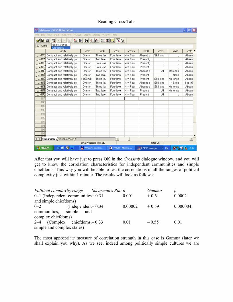
After that you will have just to press OK in the Crosstab dialogue window, and you will get to know the correlation characteristics for independent communities and simple chiefdoms. This way you will be able to test the correlations in all the ranges of political complexity just within 1 minute. The results will look as follows: Political complexity range Spearman's Rho p Gamma p 0–1 (Independent communitiesand simple chiefdoms)

+ 0.31 0.001 + 0.6 0.0002

0–2 (Independentcommunities, simple and complex chiefdoms)

+ 0.34 0.00002 + 0.59 0.000004

2–4 (Complex chiefdoms,simple and complex states)

– 0.33 0.01 – 0.55 0.01

The most appropriate measure of correlation strength in this case is Gamma (later we shall explain you why). As we see, indeed among politically simple cultures we are

Chapter 6

15

dealing with a rather strong positive correlation, whereas among politically complex cultures we encounter quite a strong negative correlation.5 We hope this example demonstrates very clearly how dangerous it is while studying a relationship to rely entirely on correlation coefficients, without a careful study of the crosstab. Now, let us read the following table (see Table 6.3): Table 6.3:

Polygyny 1 = absent 2 = occasional3 = general

TOTAL

0 = No levels(Independent communities)

75 14.9%

236 46,8%

193 38,3%

504 100%

1 = One level (Simplechiefdoms)

27 8.0%

107 31.8%

203 60.2%

337 100%

2 = Two levels(Complex chiefdoms)

20 12.7%

41 26.1%

96

157 100%

3 = Three levels(Simple states)

27 32.1%

23 27.4%

34 40.5%

84 100%

Political Centralization Index = # of Political Integration Levels over Community

4 = Four or more levels(Complex states /empires)

13 50.0%

10 38.5%

3 11.5%

26 100%

TOTAL 162 417 529 1108 While doing this, let us follow generally the instructions for reading the previous table. Note, however, that to read the new table is a bit more difficult than to read the previous one. The point is that the dependent category in the previous Table 6.2 was dichotomous, alternative, it had only two values, whereas in Table 6.3 it has three. Hence, in this table it turns out to be insufficient to describe just one category in every row. For example, the first row could be described ("read") in the following way:

"Among cultures with the lowest level of political centralization the most frequent pattern is the occasional polygyny; it occurs in almost half of such cultures. The general polygyny is also rather frequent – it is observed among a little less than

5 Note that this negative correlation is to a considerable extent accounted for by the Galton (network autocorrelation) effect produced by the functioning of the Christian and (to a lesser extent) Hinayana Buddhist historical networks (see Korotayev 2003).

Reading Cross-Tabs

40% of such cultures. Monogamous cultures only constitute around 1/6 – 1/7 of the whole subsample. However, as we shall see below, even this is not little."

The situation would be also different as regards the description of the difference between different rows. With respect to the previous table it was sufficient to describe differences within a single column. However, with respect to tables of the new type you would have to describe every column. The possible ways of doing this with respect to the table under consideration could be specified as follows:

"With the appearance of the first political integration level over community (i.e. with the formation of simple chiefdoms and equivalent polity types) we observe a considerable growth of the proportion of cultures with general polygyny – among this type of cultures almost two thirds of cases are characterized by general polygyny, and this pattern is most typical for chiefdoms. The proportion of cultures with occasional polygyny declines, this pattern is observed in less than third chiefdoms of the sample. The proportion of monogamous cultures decline almost twice – it is among simple chiefdoms where monogamy is observed most rarely."

Now, try to read the rest of the table yourself. After doing this, answer the following questions: 1. With what general type of relationship are we dealing in Table 6.3 – lineal, or curvilineal? The statistical analysis of Table 6.3 would yield the following results:

Rho = + 0.08, p = 0.005 Cramer's V = 0.21, p = 0.0000000000000001

2. Why is the value of V in our case higher than the one of Rho? 3. Why does Spearman's Rho suggest the presence of a significant positive correlation between political centralization and polygyny?