Critical Thresholds for Sediment Mobility in an Urban Stream
47
Georgia State University ScholarWorks @ Georgia State University Geosciences eses Department of Geosciences 8-1-2011 Critical resholds for Sediment Mobility in an Urban Stream Ross H. Martin Follow this and additional works at: hp://scholarworks.gsu.edu/geosciences_theses is esis is brought to you for free and open access by the Department of Geosciences at ScholarWorks @ Georgia State University. It has been accepted for inclusion in Geosciences eses by an authorized administrator of ScholarWorks @ Georgia State University. For more information, please contact [email protected]. Recommended Citation Martin, Ross H., "Critical resholds for Sediment Mobility in an Urban Stream." esis, Georgia State University, 2011. hp://scholarworks.gsu.edu/geosciences_theses/37
Transcript of Critical Thresholds for Sediment Mobility in an Urban Stream

Georgia State UniversityScholarWorks @ Georgia State University
Geosciences Theses Department of Geosciences
8-1-2011
Critical Thresholds for Sediment Mobility in anUrban StreamRoss H. Martin
Follow this and additional works at: http://scholarworks.gsu.edu/geosciences_theses
This Thesis is brought to you for free and open access by the Department of Geosciences at ScholarWorks @ Georgia State University. It has beenaccepted for inclusion in Geosciences Theses by an authorized administrator of ScholarWorks @ Georgia State University. For more information,please contact [email protected].
Recommended CitationMartin, Ross H., "Critical Thresholds for Sediment Mobility in an Urban Stream." Thesis, Georgia State University, 2011.http://scholarworks.gsu.edu/geosciences_theses/37
CRITICAL THRESHOLDS FOR SEDIMENT MOBILITY IN AN URBAN STREAM
by
ROSS HAMILTON MARTIN
Under the Direction of Jordan Clayton
ABSTRACT
Bed load transport measurements were made in a small urban stream in Decatur,
GA, from which thresholds for motion were calculated using methodologies from the
published literature. These methodologies are discussed in terms of their limitations and
assumptions. Mobility frequencies were calculated for single grains of each grain size
fraction to illustrate the transition from size selective transport to equal mobility. In
general, urban streams behave differently than many gravel rivers in non-urban settings
because of differences in the availability and character of sediment sources and altered
flow hydrographs. This comparison allows for discussion about the way sediment is
transported in urban streams versus typical gravel-bed, armored channels.
INDEX WORDS: Sediment transport, Fluvial geomorphology, Shields stress

CRITICAL THRESHOLDS FOR SEDIMENT MOBILITY IN AN URBAN STREAM
by
ROSS HAMILTON MARTIN
A Thesis Submitted in Partial Fulfillment of the Requirements for the Degree of
Masters of Science
in the College of Arts and Sciences
Georgia State University
2010

Copyright by
Ross Hamilton Martin
2011

CRITICAL THRESHOLDS FOR SEDIMENT MOBILITY IN AN URBAN STREAM
by
ROSS HAMILTON MARTIN
Committee Chair: Jordan Clayton
Committee: Seth Rose
Daniel DeoCampo
Electronic Version Approved:
Office of Graduate Studies
College of Arts and Sciences
Georgia State University
August 2011

iv
Table of Contents
List of Figures v
Introduction 1
- Urbanization and Sediment Mobility 2
- Hydrography 3
- Characteristics of Bedload Source Material 5
- Thresholds for Motion 6
This Study
- Location 10
- Topographic Surveying 11
- Sampling 12
- Transformation into common variables 13
- Transport relations 15
- Comparing Thresholds 15
- Mobility Frequency
Results
- Location Results 19
- Transport Results 21
- Shear Stress and τ* Results 22
- Comparison of critical τ* between this study and previous work 24
- Mobility Frequency 26
Discussion
- Implications on Stream Urbanization 25
- Implications on Equal Mobility 33
Conclusion 34
References 36

v
List of Figures
Figure 1. Study reach location and watershed boundary 10
Figure 2. Hydrograph of a typical event from October 7th
2008 11
Table 1. Grain Size Classification 13
Figure 3. Helley-Smith sediment sampler. 14
Table 2. Components of some critical shear stress equations, and methodology type. 18
Figure 4: Stream Morphology. Water flows from bottom to top. Contour interval is 1ft. 21
Figure 5. Pictures of study reach during low flow and ~3/4 bankfull 22
Table 3. Stream Characteristics 22
Table 4. Bedload sample conditions and results. 23
Figure 6: Grain size frequency distribution in bed load samples. 24
Figure 7: Relationship between critical Shields stress and bed load 24
Figure 8: Theoretical bed load entrainment values per size fraction using equations in Table 2 27
Table 5. Probable grain size volumes 28
Figure 9: Mobility Frequency in seconds and grain size in millimeters. 29

1
Introduction
The movement of sediments across a landscape will determine how the landscape
evolves over time. This can have huge implications in many fields of study across a range
of temporal and spatial scales. Landscape evolution on a large scale can dictate where
populations congregate, while sediment mobility can determine habitat viability for many
species. The quantification of landscape evolution via sediment transport is an important,
and long-standing goal of earth science.
Fluvial environments are a major, if not the primary, contributor to the evolution
of a landscape. Rivers and streams mobilize sediment as the flow increases and
overcomes a threshold in the balance of forces keeping sediment grains on the bed and
the shear force placed on the grain by the flow of water. Determining the ratio of these
forces for a variety of field conditions and configurations is the goal of many studies (see
Buffington and Montgomery, 1997 for an exhaustive list of incipient motion studies).
Estimates for the critical thresholds for mobility vary greatly depending upon the study
environment and methodology which created the equation.
The variation in critical thresholds for sediment entrainment in gravel rivers
comes from the different methodologies employed and variation in stream environment.
There is a relatively large range in reported threshold values that could arrive from
differing experimental or natural conditions (such as bed textural effects) and definitions
for sediment entrainment (such as particle rotation, full discussion follows in subsequent
sections) (Tison 1953; Miller et al. 1977; Carson and Griffiths 1985; Lavvelle and
Mofield 1987; Wilcock 1988; 1992; Buffington and Montgomery, 1997). Thus, estimates

2
of critical shear stress are difficult to interpret if the goal is to explore and understand
trends in sediment transport. Given the common dependency of entrainment threshold
estimates on environmental and observational characteristics, it is useful to explore
alternative ways of assessing sediment transport thresholds that are objective and
transferable to locations outside the study realm. A new way to visualize and quantify
sediment entrainment and transport must overcome the problems with threshold estimates
that cause the greatest degree of uncertainty. This research effort will explore new ways
to discuss entrainment and transport in terms of mobility frequency, which can be thought
of as a recurrence interval for the mobilization of specific grain size fractions. A review
of historical efforts to quantify sediment motion will set the context for this study and
provide a basis for understanding the significance of this study.
This study explores sediment mobility in an urban stream and seeks to reveal
some insight into urban stream transport processes using the mobility frequency
framework. Understanding the patterns of transport will lead to understanding of the
stream evolution that occurs with and urbanizing watershed.
Urbanization and Sediment Mobility
As a watershed undergoes urbanization several things occur concurrently which
affect the sediment transport mechanics in streams. The initial phase of urban
development is characterized by two to ten fold increases in sediment mobilization
(usually from disruptions in the watershed) which results in deposition in the channels,
This is followed by a phase which sees a reduction in sediment yield concurrent with
increased runoff which results in increased erosion and enlarged channels (Chin 2006).

3
Stream morphology changes with urbanization in response to concurrent changes in
sediment yield and hydrologic conditions (Paul and Meyer 2001). The influence of these
two factors vary independently in both time and intensity, while they concurrently affect
morphology- as such there are a myriad of stream morphologies (Mollard 1973; Schumm
1985; Church 2006).
Hydrography
The type of flow regime present in streams will affect how often and for how long
sediments become entrained. On one end of the spectrum are perennial mountain streams
which experience seasonal flooding, and at the opposite end of the spectrum there are
ephemeral streams in desert environments which experience very flashy hydrographs
only after storm events (Cao et al. 2010). Urban streams exist somewhere in the middle
of these two extremes, evolving towards the flashier ephemeral stream end of the
spectrum as urbanization covers more of the watershed. The majority of urban streams
are perennial, but they tend to experience events with a flashy hydrograph, similar to
ephemeral streams (Chin, 2006). It is during these flashy events that most of the sediment
transport occurs in urban streams. It is therefore important to understand how the and if
the hydrograph of a stream will affects sediment transport when using sediment transport
models.
The mechanics of sediment transport require that a certain critical shear stress be
exceeded by the flow of water for each grain size present, in order for that sediment to
become mobilized (Shields 1936). The rate at which these critical stresses are exceeded
for progressively larger grain size fractions is central to the discussion about how

4
hydrograph characteristics might change sediment transport and initial motion. A
seasonally flooding mountain stream will exceed the critical values for certain grain sizes
for long periods of time. The rate of increase and consequent decrease in shear stress
associated with the rising and falling limbs of the hydrograph is slow or subdued (Chin
2006). Therefore theoretically, a relatively larger portion of a particular grain size can be
mobilized before the shear stress increases enough so that the next larger grain size
becomes entrained. This pattern may be reduced by the effect of armoring, but here it is
important to consider the transport capacity of different shape hydrographs
independently.
Urban streams experience flashy hydrographs which translates into a sediment
transport system in which the rate of increase in shear stress is relatively fast. This means
that as one grain becomes entrained the next largest grain size will become mobilized
shortly thereafter. So, if the influence of the transported material and stream bed surface
is held constant, the shape of the hydrograph can dictate extremely different transport
environments. Urban streams can be typified by having a flashy hydrology, as the
flashiness of the hydrograph is largely dependent on the amount of impervious surface
cover present in the watershed. There are multiple other factors that can affect urban
streams, but of principle importance is that when watersheds become urbanized the
hydrographs of the affected streams or rivers will become flashier (Leopold 1968; Chin
2006). It is therefore important to explore how a flashy, urban hydrograph will affect
sediment transport. This research effort presents data from only one urban stream (for a
basin with a moderate level of imperviousness), and therefore is not able to assess how
varying degrees of urbanization affect sediment transport. Instead the research presented

5
here provides a novel method for visualizing and exploring sediment transport that will
allow future research efforts to examine the rate and character of sediment mobilization
in similar environments.
Characteristics of Bed load source material
As watersheds undergo urbanization, not only does the hydrograph change, but
sediment source material also changes. The sediment for most streams originates both in
the watershed and from in-stream sources. As a watershed becomes urbanized, sediment
sources progress in size, type and there is a shift in the mean and standard deviation of
the size fractions present. (Wolman 1967; Trimble 1997; Paul and Meyer 2001; Chin
2006). As the land is initially disturbed in processes associated with urbanization, a
proportionally large amount of fine sediments are introduced (Chin 2006). Jackson and
Beschta (1984), Ikeda and Iseya (1988), and Curran (2007) found that an increase in fine
sediments in a flume setting caused an increase in transport capacity. While this tendency
may appear counterintuitive, it may be explained in that increased amounts of fine sand
in the source material caused both bed material and slope to change so that equilibrium
transport was maintained (Curran 2007). The bed surface before the addition of fines
(from urbanization) consisted of some sand and pebble clusters which in effect caused a
large portion of the total shear stress to come from form drag with the total shear stress
being relatively low (Curran 2007). As more sand was introduced the bed surface became
smoother and the slope lessened. The reduction in the slope and the associated lower bed
shear stress coupled with increased rates of sand transport yields lower reference shear
stresses (Curran 2007). Thus, the texture of the stream bed surface can affect changes in

6
critical shear stress, which occur concurrently with changes in the hydrograph. This
creates a feed back loop where the critical threshold of large amounts of sand has been
lowered, and flow events are able to mobilize that sand more quickly because of the
increase in slope of the rising limb (i.e. flashiness) of the hydrograph. This provides a
mechanism for rapidly moving sediments (and the effects of urbanization) downstream.
When the sediment source is cut off after the initial phases of urban development, the
lowered critical shear stresses and flashiness continue to exist, which causes rapid erosion
and geomorphic degradation (Paul and Meyer, 2001).
Thresholds for Motion
For decades, there have been attempts to estimate critical thresholds of incipient
motion for bed load sediments in rivers, with notable early contributions from Gilbert
(1914), Nikuradse (1933) and Shields (1936). Buffington and Montgomery (1997)
document four general methodologies which have been employed to approximate
thresholds for incipient motion. Each has an environment for which the particular method
is best suited (Buffington and Montgomery, 1997). These methods include: [1] The
extrapolation of measured transport rates to negligible values (Shields 1936, Day 1980,
Parker and Klingeman 1982); [2] visual observations where a researcher will document
the depth (which will be used to calculate a shear stress) at which grains are seen to
mobilize, in either natural settings or flumes (Gilbert 1914, Kramer 1935, Yalin and
Karahan 1979); [3] the development of theoretical thresholds rooted in physics, where the
force of the water on the grain must exceed the force needed to rotate the grain enough to
move the grain from its initial position, in either uniform or mixed-bed rivers (White

7
1940, Wiberg and Smith 1987, Jiang and Haff 1993); [4] and finally development of
relationships based on the largest mobile grains (Andrews 1983, Carling 1983, Komar
1987). As discussed in subsequent paragraphs, the shortcomings of each method vary
from bias toward larger grains because of the sampling procedure to the inability to
gather the necessary data. It is important to consider the suitability of each method for a
particular field setting and research goal.
First, the method of extrapolating measured transport rates to negligible values
requires several transport samples to be taken before relationships can be established. The
deficiency with the first methodology is that the resulting relationship is highly dependent
upon what is considered a negligible transport rate (Wilcock 1988; Buffington and
Montgomery 1997). The volume and time and space about which transport would be
considered is crucial. A given volume X in transport can be considered initial motion, but
it is crucial to acknowledge that the same volume may not necessarily represent initial
transport if the time and space values of the observation are different. For example,
consider the difference if volume X is transported over a large area in a long time period
versus a short time and small space. The method of deriving a threshold for motion based
on visual observation relies on the subjective eye of an individual over a varying, and
often unstated, area and time in order to document when initial mobility occurs
(Buffington and Montgomery 1997). The time and space about which initial motion is
considered is therefore crucial when defining initial motion. By not understanding the
spatial and temporal constraints of a threshold methodology, one reduces the accuracy of
the transport estimates.

8
The third type of methodology described is the development of theoretical
thresholds based upon the physics of grain pivot angles, bed slope, and friction and lift
forces (Miller and Byrne 1966; Coleman 1967; Wiberg and Smith 1987; Buffington et al.
1992). It is very likely that this type of approach would be able to very precisely
determine critical threshold values, if the proper data are available. The type of data this
method requires varies greatly- even within river reaches- and is therefore difficult to
assess. For example, assumptions must be made for values of pivot angles, a parameter
upon which critical threshold value is highly dependent (Wiberg and Smith 1987). The
pivot angle of a grain is the amount a grain must rotate upon a horizontal axis in order to
move out of the place where it rests. This angle is determined by the diameter of the grain
itself and the diameter of the surrounding grains. For example a larger grain surrounded
by much smaller grains would have a small pivot angle, while a small grain surrounded
by large grains would have high pivot angles. Obviously, estimating pivot angles for a
heterogeneous bed can be quite difficult. Theoretically determined thresholds for motion
are limited by the difficulty in supplying the research effort with sufficiently accurate
field data.
The final methodology relies on the transport rates of the largest mobile grains to
create a relationship between grain size and incipient motion thresholds. By assuming the
largest grains captured during a sampling event are at or near their threshold for motion,
one can define a relationship between a critical shear stress and grain size. This method is
highly sensitive to sampling methodology and coarse grain availability (Wilcock 1992;
Wathen et al. 1995; Buffington and Montgomery 1997). While this method assumes that
coarser grains are preferentially transported by higher flow strengths (selective transport)

9
(Wilcock 1988, 1992; Buffington and Montgomery 1997), it does not necessarily
preclude a transport relation with a very steep slope (i.e. a transport close approaching
equal mobility). This contradiction shows that more research is needed to understand
how this methodology is affected by the extremes of transport relationships.
Selective transport occurs where the flow disproportionately transports certain
size fractions; typically, the competent grain size monotonically increases with flow rate
(Clayton, 2010). The opposite condition would be described as equal or full mobility,
where transport occurs for all size fractions equally proportionate to their respective
abundance on the bed (Parker et al, 1982; Wilcock and McArdell, 1993). As the
discharge of a stream increases it can transition from size selective transport to equal
mobility (Ashworth and Ferguson, 1989; Clayton and Pitlick, 2007).
Each method produces equations which will be more suited to one environment
than another. It is therefore important to explore how each type of initial motion
calculation reflects the continuum of transport environments, ranging from equal mobility
to size selective transport. The ongoing exploration of each of the different methods in a
range of environments has required, and will continue to require, copious amounts of data
and time. This study, instead, looks at the motion of sediments in a new way, where the
initiation of movement is considered in the terms of a recurrence interval. A recurrence
interval depicts the time lag between an event occurring and re-occurring. Recurrence
intervals are more familiarly used for large scale events such as floods and earthquakes.
This study describes the movement of individual grains in a similar fashion.

10
This Study
Location
Peavine Creek is a small, urbanized stream in Decatur, Georgia, located in the
Chattahoochee River watershed, in the Atlanta metropolitan region.
Figure 1: Study reach location and watershed boundary.
Peavine Creek shown in Figure 1 was selected for this study because: 1) it
exhibits a typical urban stream morphology with low width to depth ratios and a flashy
hydrograph (Paul and Meyer 2001), 2) it is small enough that bed load sampling 3) flow

11
measurement could safely be undertaken during competent events by one person, and 4)
it was close enough to be accessed quickly during storm events.
Previous unpublished research documented many aspects of Peavine Creek. A
pressure transducer placed in the stream shows that stream exhibits a typical urban
hydrograph, as seen in figure (2).
Figure 2. Hydrograph of a typical event from October 7
th 2008
There is low vegetation density on the banks, mostly grasses and shrubs. The
entire watershed is covered with a loamy soil comprised of almost equal parts of sand, silt
and clay (USDA 2010). The entire area is underlain by mica schist and gneissic rock
(USDA 2010). The watershed has undergone urbanization and reached stability,
meaning that currently there is very little to no active construction in the watershed
(USDA 2010). This is important because as land use changes are occurring, the processes
involved can introduce sediments into the stream (Trimble 1997).
12
Methodology
Topographic surveying
The current morphology of the stream reach was measured using a Nikon total station
and prism rod. These data enabled the calculation of bankfull width which is the width of
the top of the maximum flow before the stream banks are overtopped, and the water
spreads out over the floodplain. The streambed width was also determined; this is the
width of the stream bed between the sharp breaks in slope leading up to the stream banks.
The water surface slope down the reach was measured in several intervals down stream
with a hand level and stadia rod.
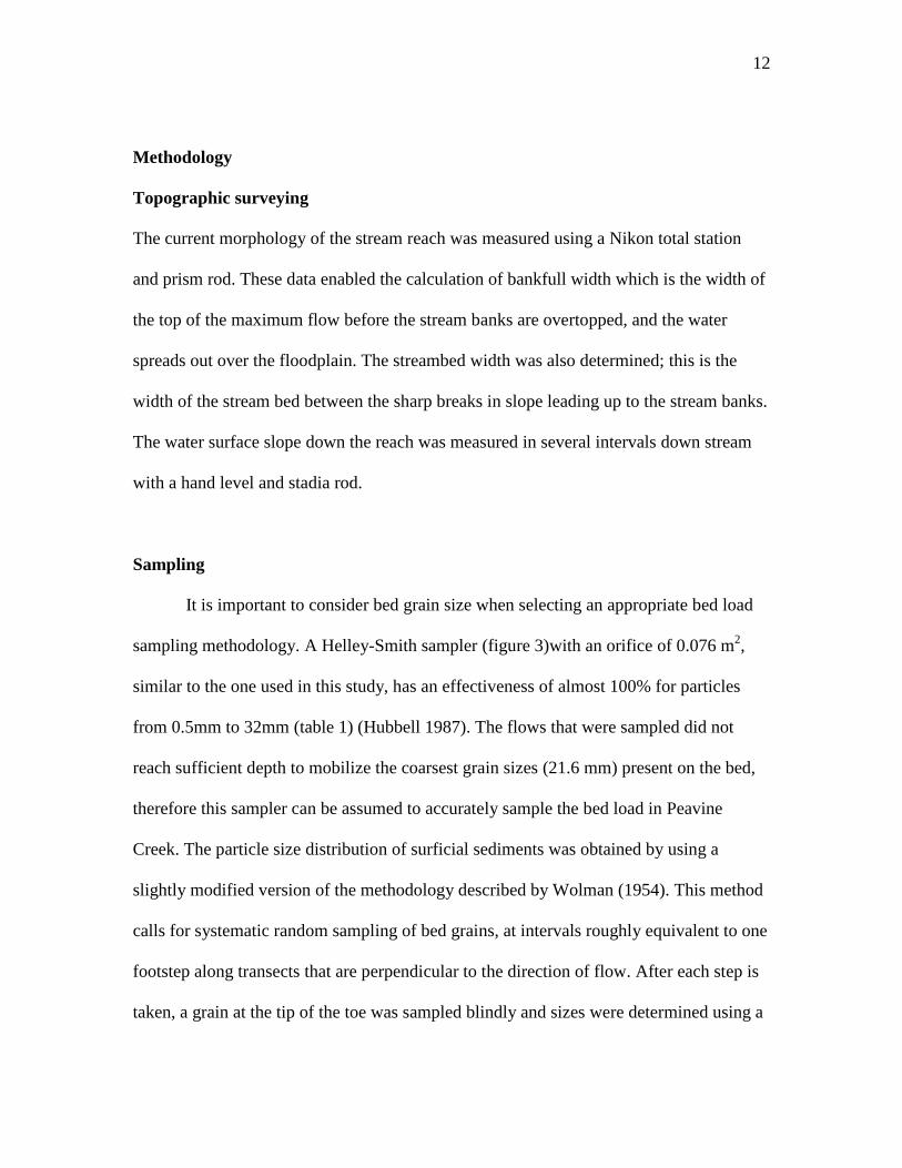
Sampling
It is important to consider bed grain size when selecting an appropriate bed load
sampling methodology. A Helley-Smith sampler (figure 3)with an orifice of 0.076 m2,
similar to the one used in this study, has an effectiveness of almost 100% for particles
from 0.5mm to 32mm (table 1) (Hubbell 1987). The flows that were sampled did not
reach sufficient depth to mobilize the coarsest grain sizes (21.6 mm) present on the bed,
therefore this sampler can be assumed to accurately sample the bed load in Peavine
Creek. The particle size distribution of surficial sediments was obtained by using a
slightly modified version of the methodology described by Wolman (1954). This method
calls for systematic random sampling of bed grains, at intervals roughly equivalent to one
footstep along transects that are perpendicular to the direction of flow. After each step is
taken, a grain at the tip of the toe was sampled blindly and sizes were determined using a

13
metal template with openings at half-phi intervals (gravelometer). This process was
repeated until 100 grains have been sampled. Six samples were taken in the study reach,
each approximately equally spaced from one another, to get an average of the entire study
reach. The grain size distributions in the stream (presented in the Results section, Figure
7) reinforce that the particle sizes present in the channel are within the appropriate range
for use of the Helley-Smith sampler.
Table 1: Grain Size Classifications

14
Figure 3: Helley-Smith sediment sampler.
Nine bed load samples were obtained in the thalweg of Peavine Creek at stages
from 0.16 to 0.36 meters (compared with 1.1 to 1.2m bankfull stage) during four
moderate flow events from the fall of 2009 to spring 2010. The sample duration was ten
minutes for each sample. The depth was monitored for the duration of the sample and if
any change in depth was observed the average of the beginning and ending depth was
used as the depth for the sample. In order to accurately characterize the stage during
sampling and to minimize the influence of unsteady flows, if the depth was seen to
increase more than 5 cm over the 10 minute time span, the sample duration was reduced;
this affected two of the samples and resulted in a sample time of 5 minutes. Samples
were taken on both the falling and rising ends of individual storm hydrographs.
Individual bed load samples were combined to assess net bed load transport and
entrainment thresholds, as this was the focus of this study.
The samples were taken to the laboratory for particle size analysis. Each of the
samples was oven-dried for up to 48 hours. Large leaf litter and other large organic
materials were removed prior to weighing and sieving the samples. Each of the samples

15
was placed into a standard Ro-tap sieve shaker which separated the samples into half phi
size fractions from coarse gravel to fine sand; silt and finer particles were combined into
a single size class. Size fractions were weighed to determine the particle size distributions
for individual samples as well as the cumulative weights per size fraction.
Transformation into Common Variables.
Once the dry weights were obtained from each sample they were transformed into
transport rates by considering several factors from the sampling event. The weight was
divided by a density of 2.65 grams per cubic centimeter to obtain a volume (Dietrich and
Smith, 1984). This volume was divided by the sampler width and sample time, which
gives the bed load transport in volume per time per unit width. Given the rectangular
channel morphology, this rate was assumed to be constant across the width of the bottom
of the channel.
Transport relations
The Einstein (1950) bed load transport parameter is a dimensionless value that is derived
from the transport volume obtained over a given sampling interval and is normalized by
the grain size. The function of the Einstein equation is to non-dimensionalize the
transport rate to allow for comparisons between studies. The transport parameter, q*, is
determined as follows:
q* = qb[(g(s-1)D3]
-1/2 (1)

16
where qb is the volumetric transport rate in cubic meters per unit width per second, g is
the acceleration due to gravity in meters per second, s is the specific gravity of the
sediment in grams per cubic meter, and D is the bed load median grain size in meters.
Defining the flow characteristics in a similar non-dimensionalized form is
necessary so that transport relations can be compared to other sites and studies. As such,
the Shields number, a dimensionless shear stress value, was obtained for each flow event,
and is calculated by non-dimensionalizing the shear stress (τ).
τ = ρghs (2)
where ρ is the density of water, h is the depth of the water, and s is the water surface
slope through the reach. For hydrostatic, fairly uniform channels, the Shields stress, τ*,
can be determined by assuming constant values for density and gravity, and dividing the
flow depth and water surface slope by the median surface grain size using the following
equation:
τ* = τ [(ρs- ρ)gD]-1
(3)
where D is the median surface grain size in meters, ρ is the density of water, and ρs is the
density of sediment (Shields 1936).
Comparing Thresholds
The Shields curve has become a standard for estimating the critical shear stress
required for particle entrainment. Barry et al. (2004) assumed a constant Shields
threshold value of 0.047, while Bagnold (1980) assumed a critical value of 0.04. A
commonly cited threshold value of Shields stress is 0.03. The 0.03 value was documented

17
by Buffington and Montgomery (1997) as being the threshold for incipient motion based
on visual assessments of coarse grained channels.
The discussion of initial motion has increasingly considered the effects of
sheltering and hiding. Relatively small particles are blocked from the full shear stress of a
stream when hidden behind a larger particle. In this instance the apparent critical
threshold for the small grain is the same as that of the larger grain or the smaller grain
appears has a higher shear stress than if it were mobilized on a homogenous bed.
Conversely, the larger surface area exposed on a larger grain may result in a lower critical
shear stress than if that same grain size was mobilized in a homogenous bed (Powell
1998; Clayton 2010). The role of relative grain size can therefore heavily influence
transport.
Assessment of particle sheltering requires evaluating entrainment based on ratios
of individual grain sizes relative to the distribution of grain sizes available on the bed.
These ratios take into account the relative homogeneity of a bed and the extent to which
larger grains effect the mobility of the smaller grains, and vice versa. In addition to
accounting for the sheltering of grains, these equations account for the greater surface
area protrusion of larger grains. Consequently, these estimates may not necessarily be
applicable for urban streams that either lack surficial armor or have a smaller range of
bed particle sizes.
Parker et al (1982) was able to establish a relationship between transport rates of
individual size fractions and threshold stresses. He was able to obtain the relationship,
τ*ci = 0.088(di/d50)-0.98
(4)

18
where di is the diameter of any grain size, d50 is the mean diameter of the subsurface
material.
Ashworth and Ferguson (1989) provide a methodology which was adapted from
Parker et al (1982). Their method provides virtually the same analysis and outcome as
Parker’s (1982), but Ashworth and Ferguson (1989) have streamlined the process and
chose to establish a relationship based upon the surficial grains instead of the subsurface
material. Ashworth and Ferguson (1989) found
τ*ci = 0.054(di/d50)-0.67
(5)
where in this equation d50 is the mean diameter of the bed surface material.
The critical Shields stress, τ*, was evaluated by using several published
equations. The equations used represent the spectrum of initial motion relationships
expressed in the Buffington and Montgomery (1997) study. These relationships (Table 2)
include several of the methodologies discussed previously.
Author
Coefficient in transport relationship
Exponent in transport relationship Methodology
Parker and Klingeman (1982) 0.088 -0.98 Reference Transport Rate (flume)
Ashworth and Ferguson (1989) 0.072 -0.65 Largest Mobile Grain
Hammond et al. (1984) 0.025 -0.6 Largest Mobile Grain
Ferguson et al. (1989) 0.047 -0.88 Largest Mobile Grain
Komar and Carling (1991) 0.039 -0.82 Largest Mobile Grain
Lepp et al. (1993) 0.149 -0.4 Largest Mobile Grain
Wilcock (1987) 0.3 -1 Reference Transport Rate
Petit (1994) 0.058 -0.66 Visual Observation
Table 2. Components of some critical shear stress equations, and methodology type.
Mobility Frequency
Another possible way to estimate sediment transport relations, and a novel aspect
of this research, is to consider the mobility frequency of transported particles. A mobility
frequency describes how often a grain is mobilized, or how often a grain moves through a

19
plane perpendicular to stream flow. To determine the mobility frequency the time it
would take to move one grain of each size fraction was calculated by dividing the
transport rates of each of the samples taken in Peavine Creek by the volume of one grain
of each size fraction. Using the Equation 6 (below), mobility frequency values were
calculated for all grain sizes for each bed load sample.
The development of the mobility frequency relation is as follows. First, it is
necessary to simplify the grain shape so that an representative particle volume may be
calculated for each grain size fraction. This study assumed that representative particle
shapes may be estimated by determining the volume for a sphere and cube of a given
radius or axis length, and taking the mean of these values to account for complexities in
the shape of natural particles. The following equation gives the average of the volume of
a sphere and a cube:
Vprob = ((3/4πR3)+(D
3)) /2 (6)
where Vprob is the probable volume of one grain, R is the radius of the grain and D is the
diameter of the grain. This equation may be used for each grain size fraction present in
the samples. The probable volume of each given grain size fraction can be divided by the
unit width and time variables to obtain a transport rate as follows:
qb = Vprob/width/time (7)
This transport rate represents the movement of one grain per the unit width and
time and has the same dimensions as the dimensional version of the Einstein parameter,
q*. Since the goal is to obtain a mobility frequency, the measured transport rate of
individual grain size fractions obtained from bed load measurements are used to solve for
time. The qb of the transported material is set equal to the minimum volume of transport

20
possible (i.e. one grain for each size fraction) which allows one to solve for the
recurrence interval time for that size fraction.
tr = qb( Vprob/Wbed)-1
(8)
where qbsample is shown above, Wbed is the stream bed width and tr is the recurrence
interval. The variable Wbed allows the equation to account for the mobility frequency for
the entire stream bed, it could be set equal to the width (from equation 7) of the sampler
bottom, or any other relevant width.
The bed load data gave transport rates in volumes per time per unit width, by
dividing the transport rate by the probable volume of a single grain one obtains a time,
which is in effect the mobility frequency. This time or mobility frequency can be thought
of in terms of a return interval, quite literally, since it describes how often a grain of a
given size should move.
This type of evaluation will show whether or not smaller size fractions can reach
equal mobility defined in mobility frequency terms (explained below), even if coarser
size fractions continue to suggest selective transport conditions. The conditions of equal
mobility and size selective transport exist on opposing ends of a continuum of transport
patterns. On one end exists equal mobility a pattern where each size fractions is
transported equally, or proportionally, relative to its abundance on the bed (Wilcock and
McArdell, 1993). The opposing condition, size-selective transport, assumes that each
consecutively-larger grain size is transported with decreasing frequency because of the
need to overcome increasingly large particle mass (Ashworth and Ferguson, 1989;
Church and Hassan, 2002). As noted previously, streams may transition from selective
transport to equal mobility as the stage increases. The changes in the shape of the

21
hydrograph associated with urban streams, as discussed earlier, makes it valuable to
understand the transport dynamics of an urban stream as it evolves and undergoes that
transformation from selective transport to equal mobility.
Results
Location Results
The survey data gathered in the previous study of Peavine Creek were used to
create the following 3-D representation of the study reach in Peavine creek. In this
representation the water would be flowing from bottom to top. Also included for
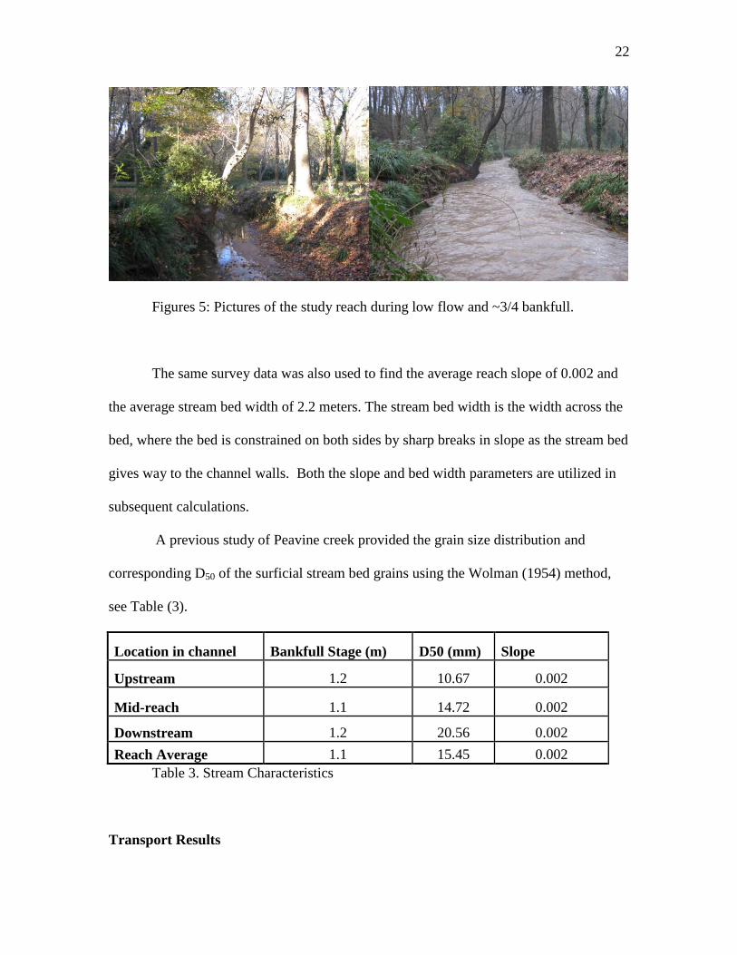
reference are pictures of the study reach during low flow and approximately ¾ bankfull
condtions (figures 4 and 5)
Figure 4. Stream Morphology. Water flows from bottom to top. Index contour
interval is 1m.
22
Figures 5: Pictures of the study reach during low flow and ~3/4 bankfull.
The same survey data was also used to find the average reach slope of 0.002 and
the average stream bed width of 2.2 meters. The stream bed width is the width across the
bed, where the bed is constrained on both sides by sharp breaks in slope as the stream bed
gives way to the channel walls. Both the slope and bed width parameters are utilized in
subsequent calculations.
A previous study of Peavine creek provided the grain size distribution and
corresponding D50 of the surficial stream bed grains using the Wolman (1954) method,
see Table (3).
Location in channel Bankfull Stage (m) D50 (mm) Slope
Upstream 1.2 10.67 0.002
Mid-reach 1.1 14.72 0.002
Downstream 1.2 20.56 0.002
Reach Average 1.1 15.45 0.002
Table 3. Stream Characteristics
Transport Results

23
The preliminary bed load transport results can be seen in Table 3. This table
describes the conditions during each sample and the total transport captured. This also
includes the transport rates used for calculating the mobility frequency.
Sample # Stage (m) Bed Width
(m) D50
(mm) qb
g/sec/width
Total Sample Volume (m^3)
Shear Stress
(Newtons) τ*
Largest Grain
Moved (mm)
1 0.17 2.3 1.6 0.50 0.01 0.324 0.014 9.5
1.2 0.24 2.3 2.0 0.92 0.02 0.473 0.021 8
2 0.25 2.1 2.2 1.68 0.03 0.498 0.022 19
2.2 0.24 2.1 1.7 1.14 0.02 0.473 0.021 8
4 0.29 2.3 2.4 1.07 0.02 0.573 0.025 13.5
5 0.37 2.1 2.6 9.40 0.16 0.722 0.032 36.5
6 0.36 2.4 2.1 6.42 0.11 0.697 0.031 19
6.2 0.42 2.4 6.8 6.76 0.06 0.821 0.036 16
7 0.30 2.3 5.6 5.35 0.09 0.597 0.026 36.5
Table 4. Bed load sample conditions and results. Here τ* is calculated using the
Shields equation (2).
These numbers describe the sampling location. If the number is followed by .2
then, that sample was the second sample in that location. Each sample was taken in the
thalweg of the channel. The bed load D50 ranges from about 0.5mm to 2.8mm. This grain
size distribution is smaller than that of the bed surface material.
The bed load material captured in each event was plotted as a cumulative
frequency or percent finer graph (Figure 5).

24
Bed Load Grain Size
0
10
20
30
40
50
60
70
80
90
10022.6
16
11
85.6
42.8
21.4
1
10.7
1
0.5
0.3
5
0.2
5
0.1
8
0.1
3
0.0
9
0.0
63
Grain Size (mm)
Pe
rce
nt
Fin
er
by
we
igh
t
1
1.2
2
2.2
4
5
6
6.2
7
Figure 6. Grain size cumulative frequency distribution in bed load samples.
Shear Stress and τ* Results
Once the shear stress (τ) on the stream was calculated the Shields stress (τ*) was
calculated for each sample event. The shear stress values are non-dimensionalized by the
mean grain size on the bed surface to obtain τ* values for each flow level.
y = 821978x3.4402
R² = 0.8102
0.0
1.0
2.0
3.0
4.0
5.0
6.0
7.0
8.0
9.0
10.0
0.000 0.005 0.010 0.015 0.020 0.025 0.030 0.035 0.040
Be
dlo
ad
Tra
ns
po
rt (
gra
ms
/se
c/w
idth
)
τ*
τ*vs. Bedload

25
Figure 8. Relationship between critical Shields stress and bed load
These values were plotted against the bed load transport rates in Figure 6. This
plot shows that there is a strong correlation between the dimensionless shear stress and
the amount of bed load material mobilized during an event. The relationship is described
by the following equation:
y=8.21978x3.4402
(9)
where x is τ* or the dimensionless shear stress, and y is the bed load transport rate in
grams/second/unit width. The R2 of the relationship is 0.81. This relationship describes
the effect of relative grain size and armoring in the coefficients and exponents. The
systematic evaluation of the variation of coefficients and exponents produced by this type
of relationship could enhance our understanding of relative grain size effects in urban
environments.
Comparison of critical τ* between this study and previous work
Many previous studies developed relations for the critical, dimensionless shear
stress per size fraction. Graphing these theoretical relations together underscores the
large range of values reported (see figure 9). These different threshold values for each
size fraction show that there is an envelope within which initial motion can occur for a
given sediment size. The results included in figure 9 are not meant to be an exhaustive
list, but rather represent the range of values common to the many initial motion equations
complied by Buffington and Montgomery (1997) and others. Since each of these
relationships is based on a ratio of grain size to the median bed surface grain size
(Di/D50), the terms of initial motion are contained within the coefficients and exponents
26
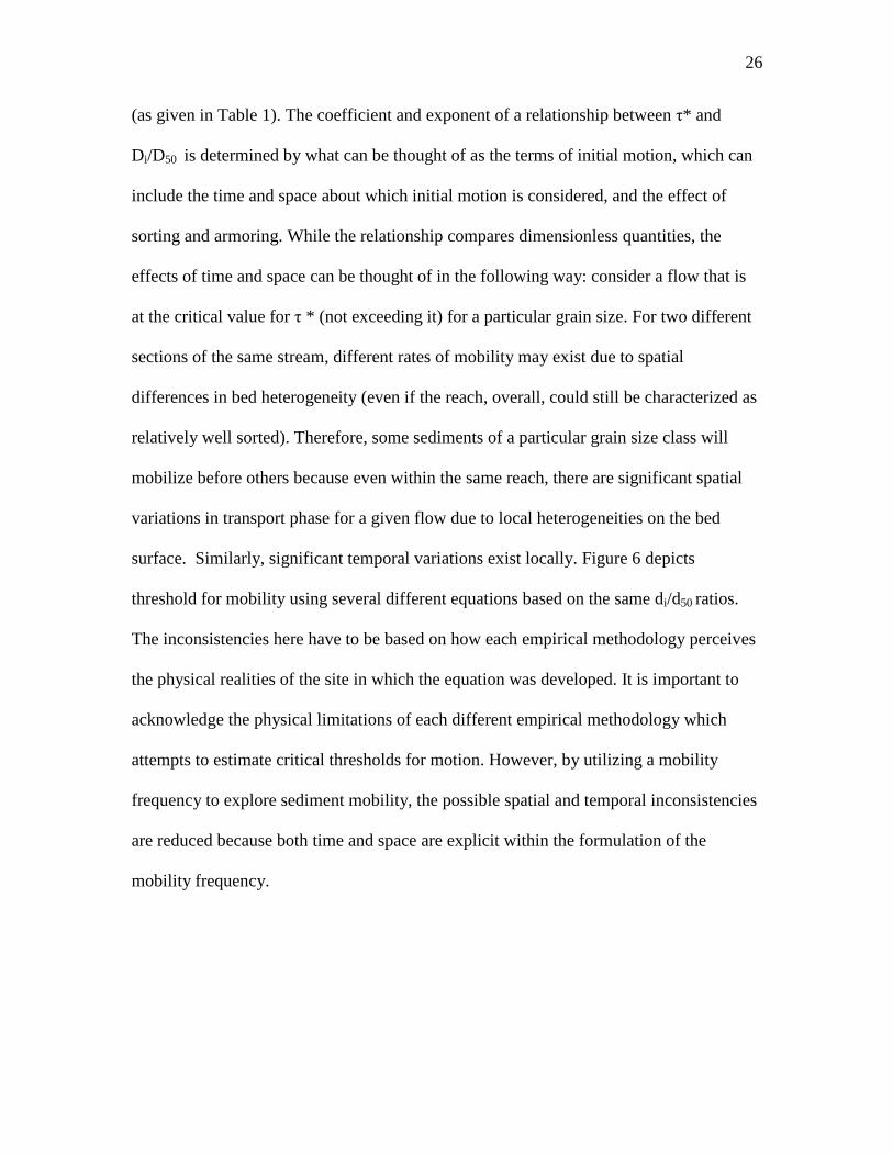
(as given in Table 1). The coefficient and exponent of a relationship between τ* and
Di/D50 is determined by what can be thought of as the terms of initial motion, which can
include the time and space about which initial motion is considered, and the effect of
sorting and armoring. While the relationship compares dimensionless quantities, the
effects of time and space can be thought of in the following way: consider a flow that is
at the critical value for τ * (not exceeding it) for a particular grain size. For two different
sections of the same stream, different rates of mobility may exist due to spatial
differences in bed heterogeneity (even if the reach, overall, could still be characterized as
relatively well sorted). Therefore, some sediments of a particular grain size class will
mobilize before others because even within the same reach, there are significant spatial
variations in transport phase for a given flow due to local heterogeneities on the bed
surface. Similarly, significant temporal variations exist locally. Figure 6 depicts
threshold for mobility using several different equations based on the same di/d50 ratios.
The inconsistencies here have to be based on how each empirical methodology perceives
the physical realities of the site in which the equation was developed. It is important to
acknowledge the physical limitations of each different empirical methodology which
attempts to estimate critical thresholds for motion. However, by utilizing a mobility
frequency to explore sediment mobility, the possible spatial and temporal inconsistencies
are reduced because both time and space are explicit within the formulation of the
mobility frequency.

27
0.001
0.01
0.1
1
10
100
0.01 0.10 1.00 10.00 100.00 1000.00
Grain Size (mm)
τ*
Parker and Klingeman (1982)
Ashworth and Ferguson(1989)Hammond et al (1984)
Ferguson et al (1989)
Komar and Carling (1991)
Lepp et al. (1993)
Wilcock (1987)
Petit (1994)
Figure 8. Theoretical bed load entrainment values per size fraction using
equations in Table 1.
Mobility Frequency
The relationship between the mobility rates for different grain size was explored by
calculating the mobility frequency for each grain size. That is done by using the existing
transport rates and the volume of a single grain. The probable volume of a given grain
size fraction is divided by the unit width, depth and time variables to obtain a transport
rate. The resulting assumed volumes of one grain of each grain size fraction used in this
study can be seen in Table 5.

28
grain size (mm) Sphere Volume (m
3) Cube Volume (m
3) Average Volume (m
3)
0.063 1.309E-13 2.500E-13 1.905E-13
0.09 3.815E-13 7.290E-13 5.553E-13
0.13 1.150E-12 2.197E-12 1.673E-12
0.18 3.052E-12 5.832E-12 4.442E-12
0.25 8.177E-12 1.563E-11 1.190E-11
0.35 2.244E-11 4.288E-11 3.266E-11
0.50 6.542E-11 1.250E-10 9.521E-11
0.71 1.873E-10 3.579E-10 2.726E-10
1 5.233E-10 1.000E-09 7.617E-10
1.41 1.467E-09 2.803E-09 2.135E-09
2 4.187E-09 8.000E-09 6.093E-09
2.8 1.149E-08 2.195E-08 1.672E-08
4 3.349E-08 6.400E-08 4.875E-08
5.6 9.191E-08 1.756E-07 1.338E-07
8 2.679E-07 5.120E-07 3.900E-07
11 6.966E-07 1.331E-06 1.014E-06
16 2.144E-06 4.096E-06 3.120E-06
23 6.041E-06 1.154E-05 8.792E-06
32 1.715E-05 3.277E-05 2.496E-05
45 4.769E-05 9.113E-05 6.941E-05
64 1.372E-04 2.621E-04 1.997E-04
90 3.815E-04 7.290E-04 5.553E-04
128 1.098E-03 2.097E-03 1.597E-03
180 3.052E-03 5.832E-03 4.442E-03
Table 5. Probable grain size volumes used in this study
The average volumes from Table 5 were used with the transport rates from each
sample event for each grain size fraction to yield a mobility frequency. The transport
rates gathered from the sampling events are in the form of a volume per time per unit
width. By setting the average volume of one grain per stream bed width equal to the
transport rates, one is able to obtain a time, which is the mobility frequency of that grain
size fraction during that sampling event.

29
0.00001
0.0001
0.001
0.01
0.1
1
10
100
1000
10000
0.01 0.1 1 10 100Grain Size (mm)
Mo
bilit
y F
req
ue
nc
y (
se
co
nd
s)
1
1.2
2
2.2
4
5
6
6.2
7
Figure 9: Mobility frequency in seconds versus bed load grain size. The different curves
represent separate bed load samples, as described above.
The mobility frequency here is similar to a recurrence interval. The lowest flows
produce the greatest frequencies; this is because lower flows have lower depths and
corresponding lower shear stress, and thus a lesser ability to move sediments. Therefore
the sediments in lower flows move sediments less frequently. If the mobility frequency
curve from a sample exists higher up the y-axis that sample has a lower recurrence
frequencies, meaning that there is a longer average lag time between the mobilization of
each individual grain from sediments of a given size class (on the x-axis). The samples
with curves lower on the y-axis are mobilizing sediment rapidly so there is a lower
mobility frequency (i.e. less time in between events). For example, if one follows a
single sample from the smallest grain size to the largest, the smaller size fractions are
lower on the y-axis which means that the smaller size fractions are moving more often

30
that the larger grains. As one proceeds to the larger grain sizes there is a notable break in
slope. The mobility frequency stays more or less the same for the lowest grain size
fractions, and then the mobility frequency decreases as the grains get larger, which is
shown by an increasing slope.
Mobility frequencies shown in Figure 10 display a pronounced break in the slope
at around 0.18 to 0.25 mm, depending on the sample. The break in slope represents a
transition from size selective transport to equal mobility because a flat trend in the
diagram (as for the finer grain size fractions) indicates that the frequency of particle
entrainment is not grain size dependent, while an increasing trend (as for the coarser size
fractions) demonstrates that increasingly coarser grains are mobilized with increasing
rarity. This suggests that the mobility frequency decreases until a threshold is reached, in
this study the threshold was about 0.2mm. The mechanics that define the transition are
unclear, and this study presents too little data to tease out a relationship. This data shows
the break of slope only occurring at two different grain sizes (0.18 and 0.25), for a
reliable threshold relationship to be found would require the slope break to occur at many
various grain sizes. The curves presented from this study are too similar for a meaningful
relationship to be created based on the threshold grain size. The threshold will likely be
quantified in the form of a ratio:
τ*/ τ*ci (10)
Where τ* is the non-dimensionalized shear stress, and τ*ci is the critical Shields value for
the grain size. Wilcock (1992) suggested a similar threshold for equal mobility (for all
sediment size fractions):
τ*/ τ*cd50 = 2 (11)

31
where τ*cd50 is the critical Shields value for the median grain size. Future research should
focus on the creation of an empirical formula that can describe the transition from equal
mobility to size selective transport. Powell (1998) noted that at transport stages this high,
fractional transport rates are a function of only their proportion on the bed surface, which
may make it necessary to also include a variable for sorting or grain availability in the
subsequent research.
By framing transport as a mobility frequency, it is possible to evaluate whether or
not, and to what extent, the transport phase of equal mobility suitably characterizes the
mobility of one or more grain size fractions. This formulation of the mobility frequency
paves the way for further exploration of the nature of equal mobility in sediment
transport, and how it changes through out a flow event. The dynamism of equal mobility
within a whole transport regime is unknown. As streams undergo urbanization, and the
hydrograph becomes flashier, the transition from size selective transport to equal mobility
could occur at different stages and for different amounts of time. It is therefore crucial to
further explore the transition to mobility frequency to full understand the urban stream
evolution.
Discussion
Implications for Stream Urbanization
The trend of the relationship between initial motion and grain size is caused by
armoring or the lack thereof. Whether or not the stream is armored is determined by the
type of flow experienced in these locations. Armored channels are characterized by a
channel in which the bed surface grains are larger on average than the underlying grains.

32
Natural (non-urban), perennial rivers receive a relatively more sustained flow and a
subdued hydrograph (Chin 2006). The other spectrum of flow type is that of urban
streams, which experience flashy hydrographs and shorter flow durations (Paul and
Meyer, 2001; Chin 2006). Once a gravel stream has adjusted to natural flow conditions it
typically has an armor layer that effectively reduces the total duration of transport for a
given flow regime. As the armoring sediments become entrained during high magnitude
flow events each size fraction may approach the condition known as equal mobility
(Powell 1998).
Urban streams cannot provide armor and therefore can not achieve equal mobility
in the same way. The flashiness of the hydrograph in urban streams precludes the
development of channel armoring because flow increases quickly enough for the
sediment to mobilize in a short period of time or the streams are able to adjust quickly
enough to the rapid changes in the hydrograph, similar to ephemeral rivers found in
desert settings (Cao et al. 2010).
It is worthwhile to consider the difference between the initial motion and final
deposition of bed grains. While initial motion describes the movement of a predetermined
amount of a certain grain size, deposition or final motion describes the last stage of the
moving particles of that amount for that grain size. The deposition process sorts those
grains as the flow decreases below the shear stress required to move the grains of a
particular size. Selective deposition may be controlled by processes similar to those that
determine particle entrainment (Powell 1998). As the hydrograph from Peavine Creek
(Figure 2) shows, the rising limb of the hydrograph has the ability to selectively entrain
sediments at a faster rate than the falling limb can selectively deposit the grains. Thus,

33
begins a cycle where the deposition of an event determines the bed surface sorting which
will in turn determine the initial motion thresholds for the next event. However those
events may be of a significantly differing magnitude, which could cause initial motion
estimates to be inaccurate. If the threshold for motion was based on a small event
preceded by a larger event, that larger event would sort the bed material differently which
may cause the threshold for motion to differ from that of an event preceded by similar
sized events.
Curran (2007) is useful in the context of this study, in that it exemplifies the
strong interaction between source material, bed surface material, and reference shear
stress for initial motion. This interaction helps to explain urban stream evolution. Curran
(2007) used flume studies allowed stream channel adjustment over a very short period of
time. In non-experimental settings, urban streams have been observed to undergo a period
of transformation (Leopold et al. 2005). This transformation consists of an initial period
dominated by aggradation followed by a period of degradation. The aggradation period
occurs as small sediments are introduced during earlier, higher intensity construction
phases of urbanization. This aggradation of fine sediments, according to Curran (2007),
effectively decreases the critical shear stress on the stream bed. This decrease in the
critical shear stress could be said to occur concurrently with the peak of active
urbanization. Active urbanization is the process which upsets the land in the watershed
and introduces sediments. At the time when active urbanization ends, there exists a lag
between end of fine sediment supply and the end of the higher transport capacities caused
by the abundant fine grains already in urban streams. As the sources of the fine sediments
have been largely cut off, urban stream bed may be experiencing prolonged lower critical

34
shear stresses due to the residual fine sediments. This concurrent reduction in fine
sediment sources and decrease in critical shear stress may help explain the rapid channel
degradation period in urban streams (Leopold et al 2005; Chin 2006).
This description of urban stream evolution shows changes in transport regime.
Theoretically, the stream begins in a nearly adjusted state, and once urbanization occurs
the stream must adjust to the new hydrologic regime and sediment sources, which also
change thoughout time. Because of the change in hydrograph and sediment sources, the
stream changes the way it entrains sediments.
Implications for Equal Mobility
Geomorphologists have coined the term equal mobility, which one would define
as the condition in which each size fraction is transported in proportion to its abundance
on the stream bed (Parker et al. 1982; Powell 1998). This condition is the counterpart of
size-selective transport which is the condition in which sediments are mobilized
proportionally to the size of the grain (Wilcock and McArdell, 1993). These two
conditions are not mutually exclusive, as shown in this study.
As streams undergo urbanization, they may evolve to an adjusted condition. An
adjusted stream is defined as a stream in which sediments are being transported and
deposited equally by any particular flow event. The concept of an adjusted stream may be
somewhat of an ideal condition that streams may never reach, but at least in concept the
sediment delivery from these stream reaches is equivalent to the sediment supply, i.e.
inputs equal outputs.
A difficult task is to understand where on the spectrum of size selective transport
and equal mobility a stream exists when it approximated an adjusted condition. This
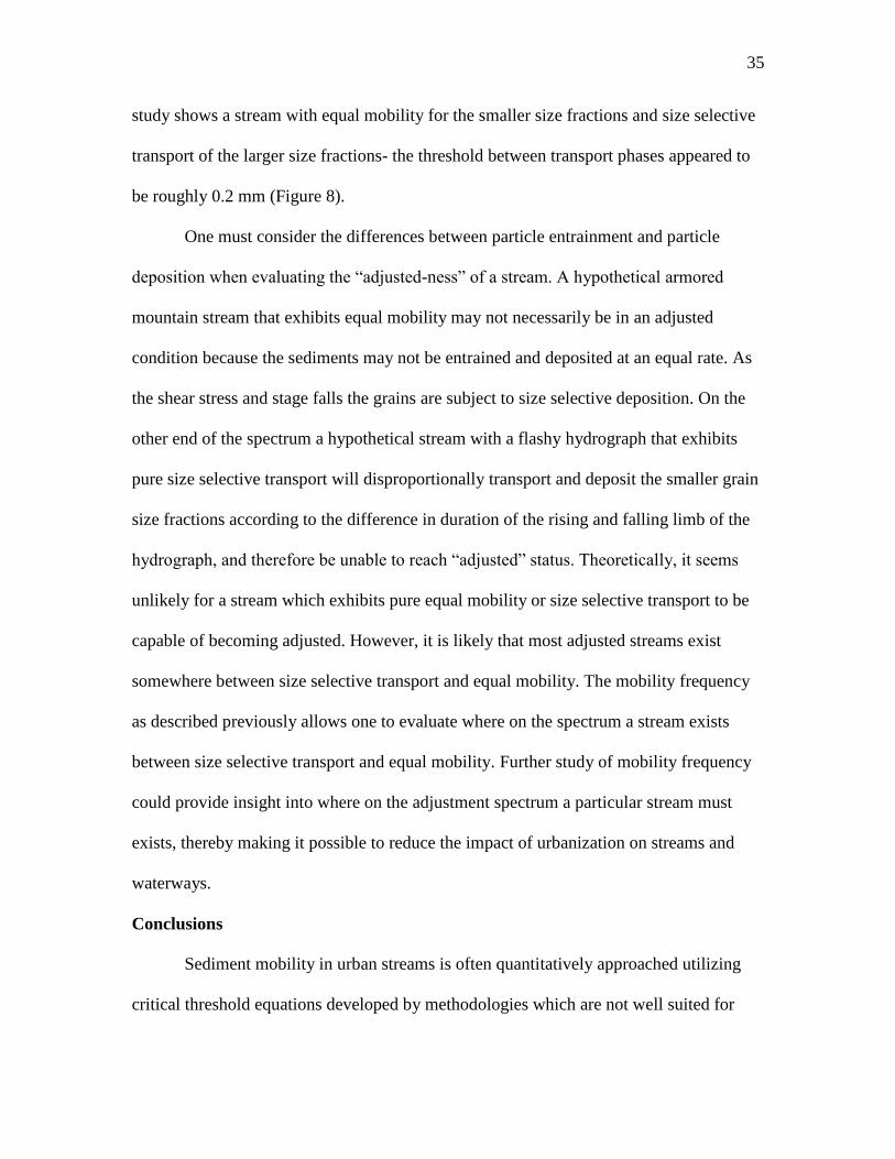
35
study shows a stream with equal mobility for the smaller size fractions and size selective
transport of the larger size fractions- the threshold between transport phases appeared to
be roughly 0.2 mm (Figure 8).
One must consider the differences between particle entrainment and particle
deposition when evaluating the “adjusted-ness” of a stream. A hypothetical armored
mountain stream that exhibits equal mobility may not necessarily be in an adjusted
condition because the sediments may not be entrained and deposited at an equal rate. As
the shear stress and stage falls the grains are subject to size selective deposition. On the
other end of the spectrum a hypothetical stream with a flashy hydrograph that exhibits
pure size selective transport will disproportionally transport and deposit the smaller grain
size fractions according to the difference in duration of the rising and falling limb of the
hydrograph, and therefore be unable to reach “adjusted” status. Theoretically, it seems
unlikely for a stream which exhibits pure equal mobility or size selective transport to be
capable of becoming adjusted. However, it is likely that most adjusted streams exist
somewhere between size selective transport and equal mobility. The mobility frequency
as described previously allows one to evaluate where on the spectrum a stream exists
between size selective transport and equal mobility. Further study of mobility frequency
could provide insight into where on the adjustment spectrum a particular stream must
exists, thereby making it possible to reduce the impact of urbanization on streams and
waterways.
Conclusions
Sediment mobility in urban streams is often quantitatively approached utilizing
critical threshold equations developed by methodologies which are not well suited for

36
urban streams. It is critical to understand the effects of each type of methodology on the
critical values produced. The goal of this study was to contextualize some insufficiencies
in current attempts to describe sediment mobility and provide a methodology which
provides new insight into sediment mobility with an emphasis on urban streams. There
exist many equations which describe the initial motion of sediments. These equations are
used to obtain a critical threshold value for motion which is often used to characterize
sediment mobility. Mobility frequencies allow a more unbiased assessment of sediment
mobility in that it can describe and compare rates and patterns of transport for the entire
spectrum of sediments present. Mobility frequencies provide a way to explore sediment
mobility that is equally able to represent transport in any environment and across scales
of magnitude.
Urban streams have very different hydrologic conditions that affect the way in
which sediment is transported and deposited. Grain size fraction mobility frequencies
developed in this study show, theoretically, how a stream might transition from size
selective entrainment to equal mobility during a storm event. Further research is needed
to understand the implication of mobility frequencies on the definitions of both size
selective transport and equal mobility. Understanding the process by which the transition
from size selective transport to equal mobility occurs might prove fundamental in
managing streams which are experiencing rapid degradation due to urbanization.

37
References cited
Andrews, E. (1983) Entrainment of gravel from naturally sorted riverbed material, Geological Society of
America Bulletin 94: 1225.
Ashworth, P, and R. Ferguson., (1989) Size selective entrainment of bed load in gravel bed streams, Water
Resources Research, 25:4.
Bagnold, R.A. (1980). An empirical correlation of bedload transport rates in flumes and natural rivers.
Proceedings of the Royal Society of London A 372(1751):453-473.
Barry, J., J. Buffington, and J. King., (2004) A general power equation for predicting bed load transport in
gravel bed rivers, Water Resources Research. 40.
Buffington, J.M. and D.R. Montgomery, (1997) A systematic analysis of eight decades of incipient motion
studies, with special reference to gravel bed rivers, Water Resources Research., 33: 1993-2029.
Buffington, J. M., W. E. Dietrich, and J. W. Kirchner., (1992). Friction angle measurements on a naturally
formed gravel streambed: Implications for critical boundary shear stress, Water Resources
Research., 28: 411–425.
Cao, Z., P. Hu and G. Pender. (2010) Reconciled bed load sediment transport rates in
Ephemeral and perennial rivers. Earth Surface Processes and Landforms 35: 1655-1665.
Carling, P. A., (1983).Threshold of coarse sediment transport in broad and narrow natural streams, Earth
Surface Processes Landforms, 8: 1–18.
Carson, M. A., and G. A. Griffiths, (1985). Tractive stress and the onset of bed particle movement in gravel
stream channels: Different equations for different purposes, J. Hydrology., 79: 375–388.
Chin, A. (2006) Urban transformation of river landscapes in a global context. Geomorphology
79: 460-487.
Church, M. and M. Hassan, (2002). Mobility of bed material in Harris Creek. Water Resources Research
38 : 1237.
Church, M. (2006) Morphology of Alluvial River Channels, Annual Review of Earth and Planetary
Sciences, 34 :325-354.
Clayton, J.A. (2010) Local sorting, bend curvature, and particle mobility in meandering gravel-bed
rivers. Water Resources Research,. 46.
Clayton, J. and J. Pitlick. (2007) Spatial and Temporal variations in bed load transport intensity in a gravel
Bed river bend, Water Resources Research. 43.
Coleman, N. L., 1967. A theoretical and experimental study of drag and lift forces acting on a sphere
resting on a hypothetical streambed, in Proceedings of the 12th Congress of the International
Association for Hydraulic Research, 3: 185–192, Int. Assoc. Hydraul. Res.,
Delft, Netherlands.
Curran, Joanna. (2007) The decrease in shear stress and increase in transport rates subsequent to an

38
increase in sand supply to a gravel-bed channel. Sedimentary Geology. 202: 572-580.
Day, T. J., (1980). A study of the transport of graded sediments, Hydraulic. Res. Stn.,
Wallingford, U. K., 190: 10.
Dietrich W.E, and Smith J.D., (1984). Bed load transport in a river meander. Water Resources Research 20:
1355–1380.
Einstein, H.A. (1950), The bed load function for sediment transportation in open channel flows, U.S. Dept.
of Agric. Soil Conserv. Serv. Tech. Bull. 1026:73.
Ferguson, R. I., K. L. Prestegaard, and P. J. Ashworth, (1989).Influence of sand on hydraulics and gravel
transport in a braided gravel bed river, Water Resources Research., 25: 635–643.
Gilbert, G.K. , (1914), The transportation of debris by running water, based on experiments made with the
assistance of E.C. Murphy: U.S. Geological Survey Prof. Paper 86: 263.
Hammond, F. D. C., A. D. Heathershaw, and D. N. Langhorne, (1984). A comparison between Shields’
threshold criterion and the movement of loosely packed gravel in a tidal channel, Sedimentology,
31: 51–62.
Hubbell, D. W.,(1987)Bed load: Sampling and analysis, in Sediment Transport in Gravel-Bed Rivers,
edited by C. R. Thorne, J. C. Bathurst, and R. D. Hey, John Wiley and Sons, New York
Ikeda, H., Iseya, F.,(1988). Experimental study of heterogeneous sediment transport. University of
Tsukuba.
Jackson, W.L., Beschta, R.L.,(1984). Influences of increased sand delivery on the morphology of sand and
gravel channels. Water Resources Bulletin 20 (4): 527–533.
Jiang, Z., and P. K. Haff, (1993).Multi-particle simulation methods applied to the micromechanics of bed
load transport, Water Resources. Res., 29: 399–412.
Komar, P. D., and P. A. Carling, (1991). Grain sorting in gravel-bed streams and the choice of particle sizes
for flow-competence evaluations, Sedimentology, 38: 489–502.
Komar, P. D., (1987). Selective grain entrainment by a current from a bed of mixed sizes: A reanalysis, J.
Sediment. Petrol., 57: 203–211.
Kramer, H., (1935). Sand mixtures and sand movement in fluvial models, Trans. Am. Soc. Civ. Eng., 100:
798–878.
Lavelle, J. W., and H. O. Mofjeld, (1987). Do critical stresses for incipient motion and erosion really exist?,
J. Hydraulic Eng., 113: 370–385.
Leopold, L. (1968) Hydrology for urban land planning – a guidebook for the hydrologic effects of urban
land use. Geological Survey Circular 554.
Leopold, L.B., Huppman, R., Miller, A., (2005). Geomorphic effects of urbanization in forty-one years of
observation. Proceedings of the American Philosophical Society 149 (3): 349–371.
Lepp, L. R., C. J. Koger, and J. A. Wheeler, (1993). Channel erosion in steep gradient, gravel-paved
streams, Bull. Assoc. Eng. Geol., 30: 443–454.
Miller, M. C., I. N. McCave, and P. D. Komar, (1977).Threshold of sediment motion under unidirectional
currents, Sedimentology, 24: 507–527.

39
Miller, R. T., and R. J. Byrne, (1966). The angle of repose for a single grain on a fixed rough bed,
Sedimentology, 6: 303–314.
Mollard JD. (1973). Air photo interpretation of fluvial features. In Fluvial Processes and Sedimentation
Proc. Can. Hydrol. Symp., 11th, Edmonton, Alberta, 1972: 341–80. Ottawa: Natl. Res. Council
Can., Comm. Geol. Geophys., Subcomm. Hydrol.
Nikuradse, J., (1950). Stro¨mungsgesetze in rauhen Rohren, Forschg. Arb. Ing.Wes., 361, 22, 1933. English
translation, Laws of flow in rough pipes, Tech. Memo. 1292, Natl. Adv. Comm. for Aeron.,
Washington, D. C)
Parker G, Klingeman P C, McLean D G (1982). Bed load and size distribution in paved gravel-bed
streams. J. Hydraul. Div., Am. Soc. Civil Eng. 108: 544–571
Parker, G., and P. C. Klingeman, (1982). On why gravel bed streams are paved, Water Resour. Res., 18:
1409–1423.
Paul, M.J. and J.L. Meyer. (2001). Streams in the urban landscape. Ann. Rev of Ecology and
Systematics, 32:333-365.
Petit, F., (1994). Dimensionless critical shear stress evaluation from flume experiments using different
gravel beds, Earth Surf. Processes Landforms,19: 565–576,
Powell, D.M. (1998). Patterns and processes of sediment sorting in gravel-bed rivers. Progress in
Physical Geography 22: 1–32.
Schumm SA. (1985). Patterns of alluvial rivers. Annu. Rev. Earth Planet. Sci. 13:5–27.
Shields, A., (1936). Anwendung der Aehnlichkeitsmechanik und der Turbulenzforschung auf die
Geschiebebewegung, Mitt. Preuss. Versuchsanst.Wasserbau Schiffbau, 26, 26, 1936. (English
translation by W. P. Ott and J. C. van Uchelen, 36 pp., U.S. Dep. of Agric. Soil Conser. Serv.
Coop. Lab., Calif., Inst. of Technol., Pasadena,)
Tison, L. J., (1953) Recherches sur la tension limite d’entrainment des materiaux constitutifs du lit, in
Proceedings of the Minnesota International Hydraulics Convention,. , Inter. Assoc.
Hydraul. Res., Delft, Netherlands,. 21–35.
Trimble S., (1997). Contribution of stream channel erosion to sediment yield from an urbanizing
watershed. Science 278: 1442.
USDA 2010, Soil Survey Staff, Natural Resources Conservation Service, United States Department of
Agriculture. U.S. General Soil Map (STATSGO2) for Georgia. Available online at
http://soildatamart.nrcs.usda.gov
Wathen, S. J., R. I. Ferguson, T. B. Hoey, and A. Werritty, (1995).Unequal mobility of gravel and sand in
weakly bimodal river sediments, Water Resources Research
Wolman, M.G., (1954). A method of sampling coarse river-bed material: Transactions of the American
Geophysical Union (EOS), 35: 951-956.
Wolman, M.G.. (1967) A Cycle of Sedimentation and Erosion in Urban River Channels, Geografiska
Annaler. Series A, Landscape and Processes: Essays in Geomorphology, Physical Geography
49( 2) : 385-395.
White, C. M., (1940).The equilibrium of grains on the bed of a stream, Proc. R. Soc. London A,

40
174: 322–338.
Wiberg, P.L, Smith, J.D. (1987) Calculations of the critical shear stress for motion of uniform and
heterogeneous sediments. Water Resources Research. 23: 1471–1480.
Wilcock, P. R., (1987). Bed-load transport of mixed-size sediment, Ph.D. dissertation. Mass. Inst.
of Technol., Cambridge, 205.
Wilcock, P. R., (1988) Methods for estimating the critical shear stress of individual fractions in mixed-size
sediment, Water Resources Research., 24: 1127–1135.
Wilcock, P. R., (1992).Flow competence: A criticism of a classic concept, Earth Surf. Processes
Landforms, 17: 289–298.
Wilcock, P. R., and B. W. McArdell, (1993). Surface-based fractional transport rates: Mobilization
thresholds and partial transport of a sand-gravel sediment, Water Resour. Res., 29: 1297–1312,
Yalin, M. S., (1977). Mechanics of Sediment Transport, Pergamon, Tarrytown, N. Y.
Yalin, M. S., and E. Karahan, (1979). Inception of sediment transport, J. Hydraul. Div. Am. Soc. Civ.
Eng., 105:1433–1443.