Crime and Welfare in South Africa 020902 - Williams … and... · 2002-09-07 · Crime and Local...

Second Draft. Comments Welcome.

Crime and Local Inequality in South Africa

Gabriel Demombynes and Berk Özler

August 22, 2002

We examine the relationship between crime and local economic welfare in South Africa.

Unlike previous studies, which use a much larger unit of analysis, we utilize data from

1066 police station jurisdictions. We find that inequality is strongly correlated with both

property crime and violent crime. Once controls for the opportunity cost and benefits of

crime participation are introduced, this correlation is substantially reduced for property

crimes, while violent crimes remain strongly associated with inequality. Returns from

crime, measured by mean per capita expenditure in the community, are strongly

correlated with property crimes, and communities that are the richest among their

neighbors experience significantly higher levels of residential burglary. Additionally,

inequality between racial groups has no association with violent crime. The results are

consistent with sociological theories that imply that inequality leads to violent crime.

They also indicate that inequality is correlated with property crime chiefly through its

association with the differential returns from such crime and that individuals may travel

to commit property crimes. Finally, the evidence presented here is at odds with the

notion that it is mainly the inequalities between racial groups that foster interpersonal

conflict.

The authors would like to thank Miriam Babita from STATS SA and Dr. Anne Letsebe from the Office of the President with help in the generation of our data set. We are grateful to Jere Behrman, Eliana La Ferrara, Peter Lanjouw, and Martin Ravallion for comments on the first draft of this paper. These are the views of the authors, and need not reflect those of the World Bank or any affiliated organization. Correspondence: [email protected] and [email protected].

2

I. Introduction

Crime is among the most difficult of the many challenges facing South Africa in

the post-apartheid era. The country’s crime rates are among the highest in the world and

no South African is insulated from its effects. Beyond the pain and loss suffered by

crime victims, crime also has less direct costs. The threat of crime diverts resources to

protection efforts, exacts health costs through increased stress, and generally creates an

environment unconducive to productive activity. Additionally, the widespread

emigration of South African professionals in recent years is attributable in part to their

desire to escape a high crime environment.1 All of these effects are likely to discourage

investment and stifle long-term growth in South Africa. Consequently, it is important to

understand the factors that contribute to crime.

Both economic and sociological theory has linked the distribution of welfare to

criminal activity. Economists have suggested that inequality may capture the differential

returns to criminal activity and thereby have an association with crime rates. If criminals

travel, not only the welfare distribution in the local area, but that of neighboring areas as

well, may be linked to local crime levels. Sociologists have hypothesized that inequality

and social welfare in general may have effects on crime through other channels.

Inequality may be associated with lack of social capital, lack of upward mobility, or

social disorganization, all of which may cause higher levels of crime. Furthermore,

1 According to a survey conducted by the South African Migration Project, blacks and whites

both “…rated security and safety as the most significant push factor, reinforcing the national importance of addressing the crime problem as a deterrent to the brain drain” Dodson (2002).

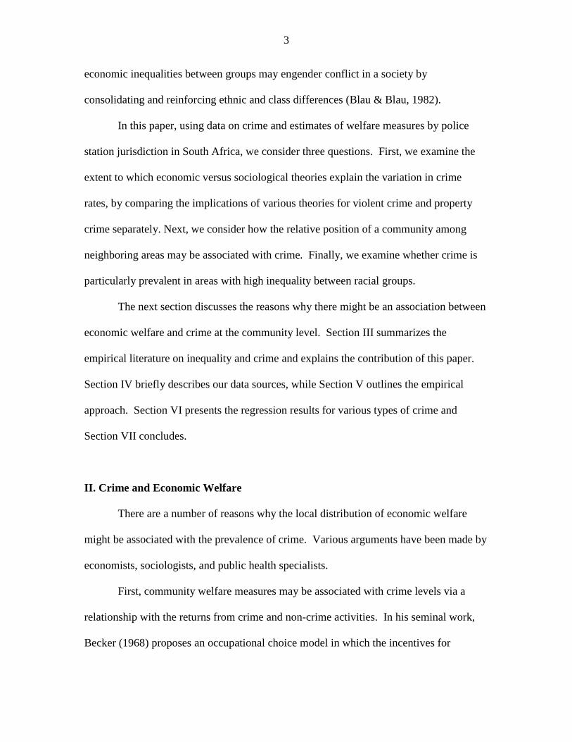
3

economic inequalities between groups may engender conflict in a society by

consolidating and reinforcing ethnic and class differences (Blau & Blau, 1982).

In this paper, using data on crime and estimates of welfare measures by police

station jurisdiction in South Africa, we consider three questions. First, we examine the

extent to which economic versus sociological theories explain the variation in crime

rates, by comparing the implications of various theories for violent crime and property

crime separately. Next, we consider how the relative position of a community among

neighboring areas may be associated with crime. Finally, we examine whether crime is

particularly prevalent in areas with high inequality between racial groups.

The next section discusses the reasons why there might be an association between

economic welfare and crime at the community level. Section III summarizes the

empirical literature on inequality and crime and explains the contribution of this paper.

Section IV briefly describes our data sources, while Section V outlines the empirical

approach. Section VI presents the regression results for various types of crime and

Section VII concludes.

II. Crime and Economic Welfare

There are a number of reasons why the local distribution of economic welfare

might be associated with the prevalence of crime. Various arguments have been made by

economists, sociologists, and public health specialists.

First, community welfare measures may be associated with crime levels via a

relationship with the returns from crime and non-crime activities. In his seminal work,

Becker (1968) proposes an occupational choice model in which the incentives for

4

individuals to commit crime are determined by the differential returns from legitimate

and illegitimate pursuits. At an aggregate level, researchers have suggested various

approaches to approximate these returns. For example, Machin and Meghir (2000) argue

that criminals are more likely to come from the bottom end of the wage distribution, and

they measure the returns to legitimate activities with the 25th percentile wage. Ehrlich

(1973) postulates that the payoffs to activities such as robbery, burglary and theft depend

on the level of transferable assets and can be proxied by median income in the

community.

Under certain conditions, a Becker-type economic model can generate a

relationship between property crime and local inequality. Suppose, for example, that the

expected returns from illegitimate activities are determined by the mean income of

households in the community. Also suppose that the returns from crime for potential

criminals are equal to the incomes of those at the lower end of the local income

distribution. Then the relative benefits of crime will be determined by the spread between

the community mean and the incomes of the relatively poor. This implies that the

expected level of crime will be greater in a community with higher inequality. Using

variations on this argument, Ehrlich (1973), Chiu and Madden (1998) and Bourguignon

(2001) all suggest that economic incentives for crimes are higher in areas with greater

inequality in the community. A Beckerian model does not imply that inequality per se

causes crime but rather that empirically inequality may capture the incentives for criminal

activity. This leaves no reason to suspect that crime should be correlated with inequality

if the costs and benefits of crime are controlled for.

5

Second, local economic welfare may also be associated with the level of

protection from crime. Private crime protection measures may include guard dogs, bars

on windows, electric fences, and alarm systems with armed security response. Chiu and

Madden (1998) provide a model that allows for richer neighborhoods to have lower crime

rates, partly because they may employ effective defense strategies against crime.

Wealthier people may also have better access to legal protection (Black, 1983). Inequality

may also be positively correlated with crime if, as Pradhan and Ravallion (1998) suggest,

concern for public safety at the household level is a concave function of income, thereby

creating a negative correlation between public concern for safety and inequality at the

aggregate level. The provision of protection from crime through collective action such as

neighborhood watch programs may also be low in communities with low social capital.

Lederman et al. (2001) suggest that social capital may decrease crime rates by lowering

the cost of social transactions and attenuating free-rider problems of collective action. If

inequality is correlated with lack of social capital in a community, then one would expect

to observe a positive correlation between inequality and crime.

Third, lack of upward mobility in the society may be linked to the prevalence of

crime. Coser (1968, cited by Blau & Blau, 1982, p. 119) argues that people who perceive

their poverty as permanent may be driven by hostile impulses rather than rational pursuit

of their interests. Wilson and Daly (1997) hypothesize that sensitivity to inequality,

especially by those at the bottom, leads to higher risk tactics, such as crime, when the

expected payoffs from low-risk tactics are poor. If income inequality, a static measure, is

correlated with social mobility, a dynamic concept, then these theories would imply a

higher prevalence of criminal behavior in more unequal areas.

6

Fourth, closely related to theories involving social mobility are those related to

social disorganization and crime. In an influential paper, Merton (1938) proposes that

“…when a system of cultural values emphasizes, virtually above all else, certain common

symbols of success for the population at large while its social structure rigorously

restricts or completely eliminates access to approved modes of acquiring these symbols

for a considerable part of the same population, that antisocial behavior ensues on a

considerable scale”. Hence, the lack of upward mobility in a society, combined with a

high premium on economic affluence results in anomie, a breakdown of standards and

values. According to Merton, poverty or even “poverty in the midst of plenty” alone is

not sufficient to induce high levels of crime. Only when their interaction with other

interdependent social and cultural variables is considered, one can explain the association

between crime and poverty.

Finally, people may be particularly sensitive to inequalities across ethnic, racial,

or religious groups, or across geographical areas.2 Blau and Blau (1982) argue that three

concepts are central to theories on social relations in a population: heterogeneity,

inequality, and the extent to which two or more dimensions of social differences are

correlated and consolidate status distinctions. For example, racial heterogeneity and

income inequality, both correlated with status in the community, could inhibit marriage

between persons in different positions or spell potential for violence. They suggest that

“… great economic inequalities generally foster conflict and violence, but ascriptive

inequalities do so particularly.” Their theory suggests inequality between racial groups

are an especially strong force behind high crime rates.

2 Kanbur (2002) argues that “…spatial units may develop special identities even without the basis of ethnicity, race or religion.”

7

What if criminals travel?

A point of departure from the literature in this paper is the incorporation of the

effects of characteristics of neighboring communities on crime. With respect to the

sociological theories of crime, such as Merton (1938), Coser (1968), and Wilson and

Daly (1997), it is not clear whether it is inequality within the community or within a

larger geographical unit that should matter in relation to crime. Next consider the

Beckerian economic theory of crime. For ease of exposition, we define “criminal

catchment area” for a neighborhood to include the neighborhood itself and all bordering

neighborhoods, while we use “own neighborhood” to refer to only the neighborhood

itself. Because individuals may travel from surrounding communities to commit crimes,

or to neighboring areas to work, the relevant returns to legitimate activities for potential

criminals (those who could commit crimes reported in own neighborhood) are the returns

available in the criminal catchment area. The relevant returns to crime, however, are

those in own neighborhood alone.

Suppose two adjoining neighborhoods are identical and have identical income

distributions, except that in one neighborhood households have incomes and transferable

assets worth twice those of households in the other neighborhood. Consequently,

inequality is equal within each of the two neighborhoods. Further suppose that

individuals can observe the mean income (or assets) of households in a neighborhood, but

not the welfare levels of individual households. In economic theories of crime, such as

Ehrlich (1973), where crime rates are a positive function of the absolute differential

returns from crime and a negative function of punishment, it is not clear why crime levels

should be higher in the richer neighborhood. When travel between neighborhoods is not

8

considered and punishment is by imprisonment only, then the effect of the difference in

mean incomes between the two neighborhoods could be zero as the returns from

legitimate and illegitimate activities, and, hence, the opportunity cost of crime are all

higher by the same proportion in the richer neighborhood.3 On the other hand, if

individuals can freely travel between the two neighborhoods at negligible cost, every

individual who allocates some time to property crime will prefer to conduct their activity

in the richer neighborhood, where the expected returns are twice as high. Thus, if

criminals can travel, economic theory predicts that crime will be higher in wealthier

neighborhoods, even controlling for inequality.

Crime rates may also be partially determined by the wealth of own neighborhood

relative to other neighborhoods in the catchment area. As above, consider a criminal

catchment area that consists of multiple neighborhoods instead of just two, where the

neighborhoods differ only in their mean level of income and assets. Then, criminals will

conduct all of their illegitimate activity in the richest neighborhood. Property crimes may

still take place in the poorer areas if travel is costly, the amount of protection from crime

varies across neighborhoods, or criminals have better information on returns from crime

in their immediate neighborhood.

The relationship between community welfare and property crime may vary with

the specific type of crime. The travel story seems best suited to explain residential

burglary, because the benefits–the value of transferable assets–are most clearly linked to

local household wealth. The travel scenario is less applicable to other property crime

3 Ehrlich (1973) argues that the changes in optimal time allocation between legitimate and

criminal activities due to such a “pure wealth effect” depends on the offender’s relative risk aversion.

9

such as vehicle theft or robbery, because the crime may take place while the victim is

away from his or her neighborhood. Consequently, wealth in the area in which the theft

is reported may not be linked to the return from crime.

In summary, a variety of theories suggest that higher inequality may be associated

with crime. Standard economic theories , which seem most applicable to property crime,

imply that inequality may be positively correlated with crime through its effect on the

differential returns from criminal activity versus legitimate pursuits. This would suggest

that there would be no relationship between crime and inequality, controlling for the

benefits and costs of crime participation. However, sociological theories of crime imply

that inequality also has a direct effect on crime. These theories suggest that inequality

leads to higher levels of both property crime and violent crime, independent of the net

returns to such crimes. Higher inequality might also lead to more crime through lower

levels of protection from crime if inequality suppresses collective action or concern for

public safety at the aggregate level.

The literature on crime does not generally address the relationship between

aggregate income levels and crime. We have argued above that if mean level of income

adequately captures the level of transferable assets in the community and individuals

travel to commit crimes, then all else equal property crime should be positively correlated

with mean income. At the same time, higher incomes may lead to lower property crime

levels through more effective protection. There is no obvious reason to expect violent

crime levels to be associated with mean income levels.

III. Crime and Economic Welfare: Empirical Evidence

10

The empirical evidence on the crime-inequality relationship, mainly based on

comparisons across countries, or states and cities in the U.S., generally shows a positive

correlation between inequality and crime. A meta-analysis of 34 aggregate data studies

(Hsieh & Pugh, 1993) shows that 97% of bivariate correlation coefficients for violent

crime with either poverty or inequality were positive, with 80% of the coefficients above

0.25. With the exception of Ehrlich (1973), who finds median income in a state to be

positively associated with property crime, studies generally do not examine the

relationship between crime and the level of household income. Ehrlich finds a positive

relationship between relative poverty (percent of population under half the median

income in the state) and crime, with higher elasticities for property crime than violent

crime. Machin and Meghir (2000) argue that higher wages at the bottom end of the

wage distribution reduce crime, while criminal activity is positively correlated with

returns from crime in the United Kingdom. Kelly (2000) finds a strong relationship

between income inequality and violent crime across US counties, but finds no such

relationship for property crime. However, he does not control for mean or median

income. Blau and Blau (1982) find that both between-race and within–race economic

inequality are associated with criminal violence across U.S. states. Lederman et al.

(2001) argue that increases in income inequality and lower growth rates lead to increases

in violent crime across countries. Using panel data for approximately 39 countries,

Fajnzylber et al. (2001) report similar findings for homicide and robbery rates across

countries. Lederman et al. (2001) also argue that higher social capital, measured using

levels of trust in each country, leads to lower rates of homicides. Kennedy, et al. (1998),

11

using data on 39 U.S. states, find that inequality affects violent crime mostly through its

effect on social capital.

There are several important limitations worth mentioning in this literature. First,

the unit of observation for which crime is examined is relatively large. The work cited

above refers mostly to cross-country studies and analyses of states and large metropolitan

areas in the U.S. It is unlikely that the underlying process that produces crime is the

same across countries. Various authors (Kelly, 2000; Chiu and Madden, 1998; Wilson

and Daly, 1997) suggest that the appropriate geographical unit to study might well be

much smaller, such as a neighborhood, rather than a state or a large metropolitan area. A

recent paper by Fafchamps and Moser (2002) looks at crime levels and its correlates in

more than 1000 communes in Madagascar but does not address the issue of inequality

and crime.

Second, comparability of definitions of crime categories and welfare indicators

poses serious problems for most cross-country studies, as does aligning data for various

countries for the same time period. For example, Fajnzylber et al (1998) use the

Deininger-Squire (1996) inequality data, the problems for which are well-documented

(Atkinson and Brandolini, 2000).

Third, most studies treat crime markets as closed, meaning that only the

characteristics of own area, and not those of neighboring areas, are allowed to influence

the crime rates. This may be a justifiable assumption when the unit of observation is a

country or a state but quickly loses appeal when geographical units are such that travel

for legitimate or illegitimate activities between them is plausible. Even the theoretical

12

work on the determinants of crime has not addressed this issue despite the fact that it is

not constrained by the availability of data for small geographical units.4

Fourth, few studies highlight the differences between the determinants of property

crime and violent crime. One exception is Kelly (2000), who argues that economic

theory is better suited to explaining property crime.

Finally, very few studies address the relative importance of economic inequality

between groups (e.g. racial or geographical groups), rather than within groups, as a

determinant of crime. One study that attempts to address this issue (Blau and Blau, 1982)

does not utilize a direct measure of within-group inequality.

In this paper, we address the limitations summarized above. The geographical

unit used in the analysis is the police station jurisdiction, which is smaller than the units

employed in empirical work that we have encountered in the literature.5 Using

geographical information for each of the police station jurisdictions, we are able to allow

explicitly for spatial effects in the analysis. The data further provides us with a detailed

breakdown of different types of crimes, defined in the same manner for all of South

Africa.6 Finally, utilizing well-known inequality decomposition techniques, we analyze

the relationship between crime and inequality within and between racial groups in South

Africa.

4 Chiu and Madden (1998) model residential burglaries with an implicit focus on small neighborhoods, but ignore the issue of possible spatial effects by citing empirical work that suggests burglars do not travel too far to commit crime. 5 The median population for a police station jurisdiction is 18,297 while the median area is approximately 227 square miles. These figures are much smaller in urban areas. 6 There may be differences in interpretation and reporting across police stations.

13

IV. Data

The data employed for the analysis comes from three main sources. First each

household in the 1996 Population Census of South Africa was matched to its local police

station jurisdiction, to generate information on household composition, race, education,

primary occupation, housing characteristics and access to services for each police station

jurisdiction. Second, crime data for 1996 were obtained from the South African Police

Service (SAPS). The crime information is a comprehensive database of crimes reported

for the entire country by police station jurisdiction.. Third, mean per capita expenditure

and per capita expenditure inequality were estimated for each police station jurisdiction

by applying a recently developed small area estimation technique to the South Africa

1996 Population Census, along with the 1995 October Household Survey and Income and

Expenditure Survey. The estimation method is described in Appendix A.

V. Empirical Strategy

Empirically, we first establish the simple correlation between inequality and

various types of crime in South Africa across police station jurisdictions. Next, we

consider whether the observed relationships are more consistent with the economic or

sociological theories of crime, by controlling for costs and benefits of crime and by

comparing the results for violent and property crimes. We also examine the effect on

crime of the relative position of a community among neighboring communities in terms

of its wealth. Finally, we analyze whether inequalities between racial groups are more

relevant in explaining crime levels than inequalities within racial groups.

14

The dependent variable for the analysis is the number of crimes reported by police

station jurisdiction. We regress crime counts by jurisdiction on inequality and a varying

set of regressors, always including jurisdiction population as a control, along with

dummy variables for each of the nine provinces in South Africa. Because crime counts

are discrete and there are zeros and small values in a non-negligible number of police

station jurisdictions, we utilize a negative binomial regression model.7

Dependent variables

We analyze six categories of property crime: residential burglary, vehicle theft,

armed robbery with aggravated circumstances, rape, serious assault, and murder.

Summary statistics for these crimes are presented in Table 1. Because theory has

different implications for property crime and violent crime, we select crimes that fall, as

much as possible, exclusively into one category or the other. Burglary and vehicle theft

are property crimes that are generally non-violent, while serious assaults and rapes are

violent crimes with no apparent direct pecuniary benefit to perpetrators.8 We also

examine two additional crimes that do not fall cleanly into one category but are often

studied in the literature: murder and armed robbery. Although both are crimes that are

violent in nature, robberies—and sometimes murders—are primarily motivated by

material gain.

Welfare indicators

7 See Greene (1997), pages. 931 – 940 for a fuller discussion of models for count data. Goodness of fit tests (as implemented in STATA) has indicated overdispersion, so we have opted to utilize a negative binomial model, of which the Poisson model is a special case.

15

The measure of inequality employed in the analysis is the mean log deviation

(Generalized Entropy inequality measure with c = 0).9 Mean log deviation takes the

following form:

)log(0 µi

ii

yfI ∑−= ,

where if refers to the population share of household i, iy is the household’s per capita

expenditure, and µ is mean per capita expenditure for the area in question.

To control for the returns from crime, we use mean expenditure in own

jurisdiction, as this will likely be highly correlated with transferable assets. One would

also like to control for the legitimate earnings opportunities for individuals who are likely

to commit crimes. We use unemployment rate in the catchment area as a proxy for the

opportunity cost of crime. We also introduce a dummy variable that indicates whether the

jurisdiction is the richest in the criminal catchment area.

We decompose our inequality measure to examine inequalities within and

between racial groups in relation to crime.10 Generalized Entropy inequality measures can

be additively decomposed into a between and within-group component along the following

lines:

jjj

jj gIgI ∑+= )]log([0 µ

µ

8 Vehicle thefts exclude carjackings. 9 We will use the median expenditure, GE(1), and the Gini Index in a future draft of this paper to test the robustness of the results to the choice of the welfare indicators. 10 In South Africa, the census allows for five “population groups”: African, White, Colored, Asian/Indian, and “other”. Due to data availability limitations, we collapse these into three separate categories—African, White, and other—which we refer to throughout the paper as “racial groups.”

16

where j refers to sub-groups, jg refers to the population share of group j and jI refers to

inequality in group j. The between-group component of inequality is captured by the first

term to the right of the equality sign. It can be interpreted as measuring what would be

the level of inequality in the population if everyone within the group had the same (the

group- average) consumption level µj. The second term on the right reflects what would

be the overall inequality level if there were no differences in mean consumption across

groups but each group had its actual within-group inequality jI .

Other explanatory variables

We test the sensitivity of the results by introducing additional control variables

that may be associated with crime levels. Population density may be an important

determinant of crime, either by increasing the supply of potential victims who do not

know the criminal, or by reducing the chances of apprehension (Kelly, 2000). Population

density is defined as the number of persons per square kilometer. We also employ the

percentage of households headed by a female, which has been used as an indicator of

instability, disorientation, and conflict in personal relations in the sociological literature

(for example, Blau and Blau, 1982). Finally, it has been suggested that youth may be

more prone to crime (Cohen and Land, 1987). We have created a variable that is equal to

the percentage of population aged 21-40 for use in the empirical models.11

Finally, we include race as a control variable. Kelly (2000) argues that race is a

predictor of crime through social isolation and feelings of hopelessness in black

11 Analysis with alternative definitions of this variable, using different age groups or only males, produced results similar to those presented in this paper.

17

communities in the U.S. Race may also be associated with other factors linked to crime.

For example, our analysis of the South Africa’s 1998 Victims of Crime Survey shows

race to be a strong correlate of private and public protection. Blacks are less likely than

those in other racial groups to have private forms of protection (alarms, high walls,

fences, armed security, guns) and also collective action (neighborhood watch).12

VI. Results

Main Results

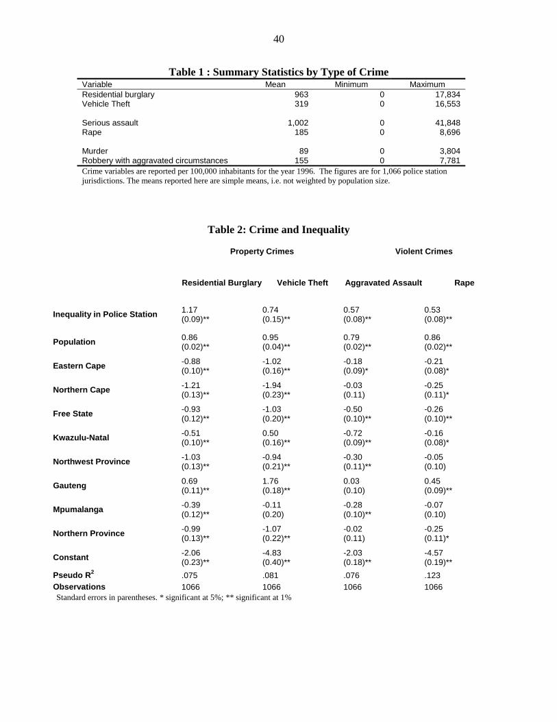
Figures 1-4 show log-log scatter plots of per capita crime levels versus inequality.

There is a positive correlation for all four crimes shown. The correlation is strongest for

property crime, particularly burglary. The same relationship is seen in the regression

results using the most basic specification, shown in Table 2. These are negative binomial

regressions with crime counts as the dependent variable and inequality, population, and

province dummies on the right hand side. Because all non-dummy variables are in log

form, the coefficients can be interpreted as elasticities. The elasticities range from 0.53

for rape to 1.17 for burglary.

The bivariate correlations between mean per capita expenditure and crime rates

are shown in Figures 5-8. Absent any additional controls, property crimes are strongly

and positively associated with average estimated expenditure in the police station

jurisdiction. The correlation between violent crimes and mean expenditure is weaker and

has somewhat of an inverted U-shape.

12 Detailed information available from the authors.

18

In the analysis shown in Table 3, we regress crime rates on inequality and mean

per capita expenditure. Adding mean expenditure greatly increase the explanatory power

of the property crime regressions, but has negligible impact on the pseudo-R-squared for

the violent crime regressions. Once mean expenditure is controlled for, the correlation

between inequality and vehicle theft completely disappears, while the coefficients on

inequality for other crimes fall substantially but remain positive and significant. The

coefficients on mean expenditure show strong relationships with property crime and a

weaker association with violent crime. The elasticities on mean expenditure for burglary

and vehicle theft, which are 0.97 and 1.77 respectively, are high relative to those for

violent crime. This is consistent with our assertation that mean expenditure per capita

may proxy the returns to property crime..

Table 4 presents results from analysis that includes an additional control for

unemployment in each jurisdiction’s criminal catchment area. In the absence of earnings

data for potential criminals, we suggest that the employment rate may capture the

opportunity cost of crime. The coefficients on inequality and mean expenditure are

virtually unchanged in this specification, while we find no association between

unemployment and crime, other than the small negative coefficient on vehicle theft,

significant only at the 10% level. These results represent our best effort to control

separately for the costs and benefits of crime for potential criminals. Clearly, the mean

expenditure and unemployment variables may have other, more complicated relationships

to crime rates. For example, unemployment may capture not only opportunity costs for

potential criminals, but also part of the value of transferable assets, and thus the benefits

of crime. An insignificant or weak negative relationship between unemployment and

19

crime is not an uncommon finding in the literature (Kelly, 2000; Ehrlich, 1973) and we

revisit the issue later in the paper.

Next we consider the impact of the rank of a jurisdiction’s wealth among its

neighbors. In Table 5, we include a dummy variable equal to one if the jurisdiction has

the highest per capita expenditure among jurisdictions in its criminal catchment area.

Controlling for inequality and mean expenditure in own jurisdiction, and unemployment

in the catchment area, burglary rates are 20% higher in jurisdictions that are the

wealthiest among their neighbors. This is consistent with the hypothesis that burglars

travel to neighboring areas where the expected returns are highest. The coefficient on the

richest jurisdiction dummy is insignificant for other crimes. The fact that we find a

significant link between a jurisdiction’s relative rank and burglary, but not other crimes,

is not surprising. There is no theoretical reason to suppose that violent crime should be

associated with a jurisdiction’s wealth, while vehicle thefts are much less clearly linked

to the characteristics of the area in which the crime is reported.

Next we examine the relationship between crime and inequality within and

between racial groups. Table 6 presents the results of the decomposition of overall

inequality in each police station jurisdiction into its within and between racial group

components. Table 6 shows that, on average, 36% of inequality in a police station

jurisdiction can be attributed to differences in mean levels of expenditure between racial

groups.

Table 7 repeats the analysis shown in Table 5, but reports parameter estimates for

within and between-group inequality, instead of overall inequality. The motivation here

is to shed some light on the hypothesis that economic inequalities between racial groups

20

are particularly important in the generation of crime, especially violent crime. The

results are surprising. Almost all of the association between inequality and levels of

crime can be attributed to inequality within racial groups. While within-group inequality

has a large and positive correlation with burglaries, assaults, and rapes, between-group

inequality has a very small correlation with burglaries and no association with any other

crimes. It is inequality among Africans, Whites, or others, and not inequality across these

groups that is most related to violent crime levels. Decomposing inequality into within

and between-group components does not substantially affect the other parameter

estimates.

Misreporting in Crime

Underreporting is a potentially seriousbut frequently neglected problem in the

crime literature. There is often the danger that the observed relationships between crime

and other variables reflect correlations with crime misreporting. It is generally difficult

to deal with this problem due to the absence of independent data on crime reporting. In

South Africa, however, the nationally representative Victims of Crime Survey (VCS) was

conducted in 1998, in which households were asked whether crimes they experienced

were reported to the police. Summary statistics for selected crimes are presented in Table

8. The definitions of the crime categories in the VCS differ from those in the SAPS data,

and hence the figures in this table are meant to be only suggestive of possible

underreporting. According to the VCS data, underreporting is a particularly serious

problem for robbery and is least serious for theft of vehicles.

21

Measurement error in the dependent variable is a problem in regression analysis

to the extent that it is correlated with some of the regressors in the model. In the case of

crime misreporting, if, for example, only wealthy people reported crime or the police

only filed official reports for complaints by the rich, then one would find a correlation

between wealth and reported crime regardless of the true relationship between wealth and

crimes committed.

To examine the extent to which misreporting effects the results presented in

Tables 2-7, we repeat the analysis using adjusted crime statistics. We conduct the

analysis exclusively for residential burglary, which, unlike other crimes, both appears

frequently in the victims survey and has nearly identical definitions in the VCS and SAPS

data. For respondents in the VCS, who said they were victims of burglary in the five

years previous to the survey, we estimate a probit regression for whether the crime was

reported to the police. We use the same explanatory variables, at the police station

jurisdiction level, as in our earlier analysis: inequality, per capita expenditure,

unemployment, and the richest jurisdiction dummy. The results of this regression are

shown in the first column of Table 9. Unemployment in the criminal catchment area is

negatively correlated with the probability of a residential burglary being reported by a

household, while per capita expenditure has a positive parameter estimate that is only

significant at the 10% level. We use the coefficient estimates from this regression to

predict, for each jurisdiction, the probability p that a burglary was reported to the police.

We then calculate an adjusted count of burglaries for each police station by multiplying

the reported number of crimes by 1/ p. Columns 2-5 in Table 9 present the results from

analysis using the adjusted burglary counts as the dependent variable for four regression

22

models previously estimated in Tables 2-6. Column 6 redisplays earlier results from the

full specification (same as column 5) using unadjusted counts as the dependent variable.

Compared with the earlier results the elasticities of inequality and per capita expenditure

are still positive and significant but somewhat attenuated, while unemployment is now

significantly and positively associated with residential burglaries. This analysis also

confirms that misreporting in crime may bias parameter estimates. Nonetheless, the

results we derive for residential burglary remain broadly the same: burglaries are more

likely to take place in wealthier areas which are unequal and in particular those which

have the highest mean expenditure among their neighbors.

Are the results robust to the inclusion of other explanatory variables?

Researchers have suggested that many factors other than economic welfare may

be related to the prevalence of crime in a community. In this subsection, we examine

whether these variables are consistently associated with crime in South Africa, and assess

whether the parameter estimates for the welfare indicators are sensitive to their

inclusion.13

Tables 10-13 present the results for each of the four crime types included in the

analysis. Percentage of individuals aged 21-40 in the jurisdiction is strongly correlated

with all types of crime, with a consistently large elasticity for all types of crime.

Population density is also significantly correlated with property crime levels, albeit the

elasticity is small. Race (measured by percentage of African households in jurisdiction)

13 Tables of pairwise correlations for these variables are shown in Appendix Table 1.

23

and percentage of female-headed households have no consistent correlation with crime

levels.

The parameter estimates for the welfare indicators are generally robust to the

inclusion of these variables in the regression models. The qualitative results are identical

for residential burglaries, i.e. they are positively correlated with mean expenditure,

inequality in the jurisdiction, and with the dummy variable for the richest community in

the criminal catchment area. With additional controls, inequality and being the richest

community have a positive but not consistently significant correlation with vehicle thefts.

Mean expenditure levels remain the strongest correlate of vehicle thefts in a community.

Regarding violent crimes, the coefficient on mean expenditure for either crime type is

unstable, once covariates are introduced. The effect of inequality in jurisdiction remains

positive and significant for both assaults and rapes, and being the richest jurisdiction

locally has no correlation with violent crime levels.

Are the results robust to the specification of functional form?

We have used a count model for the regression analysis of crime levels, with a

control for population. However, some researchers have utilized OLS regressions for

similar analysis of crime rates (typically, crimes per 100,000 individuals). To test the

sensitivity of the results to the regression specification and to better compare the results

to others in the literature, we reestimate the models using an OLS specification,

regressing log crime rates on logs of the same explanatory variables.

Table 14 presents the results for our most basic specification, in which only

inequality is considered. Inequality is still strongly associated with all crimes, but the

24

elasticities are consistently higher using OLS regressions. Table 15 shows that,

conditional on mean per capita expenditure, inequality is positively associated with all

crimes except vehicle thefts with the elasticities again substantially larger than those from

the negative binomial regressions. The association between mean expenditure and

property crime is the same as before, while the small positive association in the earlier

models between mean expenditure and serious assault disappears. Furthermore, adding

unemployment in the criminal catchment area and a richest jurisdiction dummy to the

regression model (see Tables 16 & 17) generates no more differences in the results.

Lastly, Table 18 presents the results of the specification where we examine the

association between crime and inequality within and between groups. Inequality within

racial groups is strongly correlated with all types of crime with consistently large

elasticities, while inequality between groups is positively correlated with burglary,

assault, and rape but the elasticities are small—all less than 0.15.

In summary, the OLS results are broadly similar to those from the negative

binomial regressions. Mean expenditure levels are strongly correlated with property

crimes, while inequality is positively correlated with all crimes with the exception of

vehicle thefts. Jurisdictions that are the wealthiest in their criminal catchment area are

more likely to experience residential burglaries than their neighbors. The association

between inequality and crime is mostly due to inequality within racial groups, although

between-group inequality may have a small association with crime as well.

Murder and Robbery

25

Many studies on crime examine murders and robberies. Murder is often studied

because it is thought to suffer least from reporting problems and is one of the most

violent crimes. Robberies are usually referred to as violent crimes as well despite the fact

that the primary motivation of a robbery is largely economic. In this subsection, we

demonstrate that while murders fit well within the general picture of violent crimes,

robberies fit much better with property crimes.

Table 19 shows the results of negative binomial regressions for murder and armed

robbery. The results for murder are similar to those for assault and rape. Murder levels

have a small positive association with mean expenditure levels and are positively

correlated with inequality. The elasticity of murder with respect to inequality within or

between racial groups is insignificant. Robbery, on the other hand, exhibits the common

characteristic of property crimes – it is highly correlated with mean expenditure in the

jurisdiction.

VII. Conclusions

Both theoretical and empirical papers in the crime literature have called for an

analysis of crime at a smaller level of geographical disaggregation than countries, states

or large metropolitan areas. When the unit of analysis is large, not only is there loss of

information regarding relative welfare levels across neighborhoods, but also the fact that

individuals may travel to conduct criminal activities is ignored. In this paper, utilizing

data on crime and welfare in all police station jurisdictions in South Africa, we have

analyzed the relationship between local welfare and crime. Although, the contribution of

this paper is mainly empirical, we have also suggested a pathway for the generation of

26

property crimes in a jurisdiction that takes into account the distribution of welfare in the

surrounding area, and not just within its own borders.

Starting with property crimes, the empirical results indicate that inequality is

highly correlated with both burglary and vehicle theft, but once mean expenditure in own

jurisdiction and unemployment in the catchment area are controlled for, this correlation

becomes smaller for burglary and disappears completely for vehicle theft. Property crime

is strongly correlated with mean expenditure in the jurisdiction, indicating that returns

from crime are major determinants of property crimes. If wealthier communities have

more effective protection from crime, the elasticity of residential burglaries with respect

to mean expenditure, controlling for protection, may be even higher. Considering the

welfare levels in neighboring jurisdictions, we show that jurisdictions that are the

wealthiest jurisdiction in their criminal catchment areas have higher levels of burglary.

That the locally wealthiest neighborhoods are hotspots for residential burglary is

consistent with the story that burglars travel based on information on welfare levels of

different neighborhoods. At the same time, that burglaries do not occur exclusively in

such areas suggests that there are travel costs, that burglars have more idiosyncratic

information regarding houses in their own neighborhood, or that the level of protection

varies between jurisdictions.

Violent crimes, our results indicate, are more likely to happen in areas with high

expenditure inequality but are not consistently correlated with mean expenditure levels.

Controlling for unemployment, mean expenditure and other covariates does not

substantially reduce the correlation between inequality and violent crime. Most of the

correlation between overall inequality and violent crimes is attributable to inequality

27

within racial groups, although between-group inequality also has a significant but very

small correlation with crime. This finding is at odds with the suggestion that

“…economic inequalities matter, but ascribed inequalities do so particularly”. (Blau and

Blau, 1982)

The results support the sociological theories of crime, especially with respect to

violent crimes. Beckerian economic theory of crime does not predict any correlation

between inequality and crime other than via a correlation with the differential returns

from such crimes. That we find a conditional correlation of inequality with burglaries

and violent crimes lends support to theories that suggest that inequality may lead to

higher crime levels through other, non-economic, channels.

Some economic and sociological theories of crime suggest that there may be a

positive relationship between poverty and crime levels. We have not explored this in our

empirical analysis, mainly because mean expenditure and poverty are very highly and

negatively correlated in our data set – the correlation coefficient is -0.87.14 The results

are robust to the inclusion of other covariates that may also be important factors in

explaining the variation in crime levels. They are also robust to the specification of

functional form. The parameter estimates for burglaries change somewhat when we

introduce a correction for underreporting, suggesting that misreporting in crime may bias

results in similar studies. However, the basic results stand. Unemployment in the

14 When poverty rate, measured by the headcount index, is included in the regression models for

burglary with inequality as the only other regressor, it has an elasticity of -0.56 that is statistically significant. Controlling for only mean expenditure, it has a positive and significant elasticity of 0.21. When all three welfare measures are included in the regression model, poverty has no correlation with burglary.

28

criminal catchment area, a proxy for the opportunity cost of crime, becomes positively

correlated with burglaries once crime counts are adjusted for underreporting.

We hesitate to draw policy implications from analysis using cross-sectional data

without a strong identification strategy, especially given that a direct indicator of the most

visible policy tool, public expenditures on crime prevention, is missing from the

empirical analysis. Nonetheless, we note the following. First, regarding prevention

efforts for various property and violent crimes, policymakers may want to focus on

different elements, as it is likely that different mechanisms are responsible for the

generation of each type of crime. Second, increasing the public supply of resources for

prevention in high property crime areas would be regressive, as these crimes are most

likely to occur in richer neighborhoods. Behrman and Craig (1987) show that

governments may care as much about equitable distribution of public resources as

marginal benefit of the extra resources spent. Finally, policies that help reduce economic

inequalities between neighborhoods within a local administration may also help reduce

property crime levels, particularly residential burglaries.

29

References

Atkinson, A.B., and Andrea Brandolini. 2000. Promise and pitfalls in the use of “secondary” data sets: income inequality in OECD countries. Banca d’Italia. Temi di Discussione. No. 379: 1-57. Babita, Miriam, Gabriel Demombynes, Nthabiseng Makhatha, and Berk Özler. 2002. Estimated Poverty and Inequality Measures in South Africa: A Disaggregated Map for 1996. Processed. Becker, Gary S. 1968. Crime and Punishment: An Economic Approach. The Journal of Political Economy. Volume 66, Issue 2, 169-217. Behrman, Jere R., and Steven G. Craig. 1987. The Distribution of Public Services: An Exploration of Local Governmental Preferences. The American Economic Review, Volume 77, Issue 1, 37-49. Black, Donald. 1983. Crime as Social Control. American Sociological Review, Volume 48, Issue 1, 34-45. Blau, Judith R., and Peter M. Blau. 1982. The Cost of Inequality: Metropolitan Structure and Violent Crime. American Sociological Review, Volume 47, Issue 1, 114-129. Bourguignon, Francois. 1998. Inefficient inequalities : notes on the crime connection. Mimeo, Delta and World Bank. Bourguignon, Francois. 2001. Crime as a Social Cost of Poverty and Inequality: A Review Focusing on Developing Countries. In “Facets of Globalization” eds. Shahid Yusuf, Simon Evenett, and Weiping Wu. Chiu, W. Henry, and Paul Madden. 1998. Burglary and income inequality. Journal of Public Economics, 69, 123-141. Cohen, Lawrence E., and Kenneth C. Land. 1987. Age Structure and Crime: Symmetry Versus Asymmetry and the Projection of Crime Rates Through the 1990s. American Sociological Review, Volume 52, Issue 2, 170-183. Deininger, Klaus W., and Lyn Squire. 1996. A new data set measuring income inequality. World Bank Economic Review. Volume 10: 565-591. Demombynes, Gabriel, Chris Elbers, Jean O. Lanjouw, Peter Lanjouw, Johan Mistiaen, and Berk Özler. 2002. Producing an Improved Geographic Profile of Poverty. Methodology and Evidence from Three Developing Countries. WIDER Discussion Paper No. 2002/39.

30

Di Tella, Rafael, and Ernesto Schargrodsky. 2001. Using a Terrorist Attack to Estimate the Effect of Police on Crime. Center for Research on Economic Development and Policy Reform Working Paper No. 90. Dodson, Belinda. 2002. Gender and The Brain Drain from South Africa. The Southern African Migration Project. Migration Policy Series No. 23. Ehrlich, Isaac. 1973. Participation in Illegitimate Activities: A Theoretical and Empirical Investigation.. The Journal of Political Economy. Volume 81, Issue 3, 521-565. Elbers, C., P. Lanjouw, J. Lanjouw, and P.G. Leite. 2001. Poverty and Inequality in Brazil: New Estimates from Combined PPV-PNAD Data. Processed. Elbers, C., P. Lanjouw, and J. Lanjouw. 2002. Micro-level Estimation of Poverty and Inequality. Econometrica. Forthcoming. Fafchamps, Marcel, and Christine Moser. 2002. Crime, Isolation, and the Rule of Law. Processed. Fajnzylber, Pablo, Daniel Lederman, and Norman Loayza. 2000. What Causes Violent Crime? Forthcoming in The European Economic Review. Fajnzylber, Pablo, Daniel Lederman, and Norman Loayza. 2001. Inequality and Violent Crime. Forthcoming in The Journal of Law and Economics. Hsieh, C., and M.D. Pugh. 1993. Poverty, Inequality, and Violent Crime: A Meta-Analysis of Recent Aggregate Data Studies. Criminal Justice Review, 18(2): 182-202. Kelly, Morgan. 2000. Inequality and Crime. The Review of Economics and Statistics, 82(4): 530-539. Kennedy, Bruce P., Ichiro Kawachi, Deborah Prothrow-Stith, Kimberly Lochner, and Vanita Gupta. 1998. Social Capital, Income Inequality, and Firearm Violent Crime. Soc. Sci. Med., Vol 47, No. 1, pp. 7-17. Lederman, Daniel, Norman Loayza, and Ana María Menéndez. 2001. Violent Crime: Does Social Capital Matter? Forthcoming in Economic Development and Cultural Change. Machin, Stephen, and Costas Meghir. 2000. Crime and Economic Incentives. The Institute for Fiscal Studies Working Paper, 00/17. Merton, Robert K. 1938. Social Structure and Anomie. American Sociological Review, Volume 3, Issue 5, pp. 672-682.

31

Mistiaen, Johan, Berk Özler, Tiaray Razafimanantena, and Jean Razafindravonona. 2002. Putting Welfare on the Map in Madagascar. Africa Region Technical Working Paper Series No. 34. The World Bank. Pradhan, Menno, and Martin Ravallion. 1999. Who Wants Safer Streets? Explaining Concern for Public Safety in Brazil. Processed. Victims of Crime Survey. 1998. Statistics South Africa. Wilson, Margo, and Martin Daly, 1997. Life Expectancy, Economic Inequality, Homicide, and Reproductive Timing in Chicago Neighborhoods. British Medical Journal, 314:1271.

Fig

ure

1: I

nequ

alit

y an

d R

esid

enti

al B

urgl

arie

s pe

r C

apit

a

residential burglaries per 100,000 individuals

Gen

eral

ized

Ent

ropy

Ineq

ualit

y M

easu

re (

c=0)

.2.5

11.

5

210100

1000

1000

0

B

oth

vari

able

s ar

e in

loga

rith

ms.

Obs

erva

tion

s w

here

res

iden

tial

bur

glar

ies

wer

e eq

ual t

o ze

ro h

ave

been

rep

lace

d by

the

smal

lest

val

ues

in th

e sa

mpl

e.

33

Fig

ure

2: I

nequ

alit

y an

d V

ehic

le T

heft

s pe

r C

apit

a

vehicle thefts per 100,000 individuals

Gen

eral

ized

Ent

ropy

Ineq

ualit

y M

easu

re (

c=0)

.2.5

11.

5

110100

1000

1000

0

B

oth

vari

able

s ar

e in

loga

rith

ms.

Obs

erva

tion

s w

here

veh

icle

thef

ts w

ere

equa

l to

zero

hav

e be

en r

epla

ced

by th

e sm

alle

st v

alue

s in

the

sam

ple.

34

Fig

ure

3: I

nequ

alit

y an

d Se

riou

s A

ssau

lts

per

Cap

ita

serious assaults per 100,000 individuals

Gen

eral

ized

Ent

ropy

Ineq

ualit

y M

easu

re (

c=0)

.2.5

11.

5

1045100

1000

1000

0

B

oth

vari

able

s ar

e in

loga

rith

ms.

Obs

erva

tion

s w

here

ser

ious

ass

ault

s w

ere

equa

l to

zero

hav

e be

en r

epla

ced

by th

e sm

alle

st v

alue

s in

the

sam

ple.

35

Fig

ure

4: I

nequ

alit

y an

d R

apes

per

Cap

ita

rapes per 100,000 individuals

Gen

eral

ized

Ent

ropy

Ineq

ualit

y M

easu

re (

c=0)

.2.5

11.

5

410100

1000

1000

0

B

oth

vari

able

s ar

e in

loga

rith

ms.

Obs

erva

tion

s w

here

rap

es w

ere

equa

l to

zero

hav

e be

en r

epla

ced

by th

e sm

alle

st v

alue

s in

the

sam

ple.

36

Fig

ure

5: A

vera

ge E

xpen

ditu

re a

nd R

esid

enti

al B

urgl

arie

s pe

r C

apit

a residential burglaries per 100,000 individuals

mea

n ho

useh

old

expe

nditu

re p

er c

apita

125

1000

2000

3000

4000

210100

1000

1000

0

Bot

h va

riab

les

are

in lo

gari

thm

s. O

bser

vati

ons

whe

re r

esid

enti

al b

urgl

arie

s w

ere

equa

l to

zero

hav

e be

en r

epla

ced

by th

e sm

alle

st v

alue

s in

the

sam

ple.

37

Fig

ure

6: A

vera

ge E

xpen

ditu

re a

nd V

ehic

le T

heft

s pe

r C

apit

a

vehicle thefts per 100,000 individuals

mea

n ho

useh

old

expe

nditu

re p

er c

apita

125

1000

2000

3000

4000

110100

1000

1000

0

B

oth

vari

able

s ar

e in

loga

rith

ms.

Obs

erva

tion

s w

here

veh

icle

thef

ts w

ere

equa

l to

zero

hav

e be

en r

epla

ced

by th

e sm

alle

st v

alue

s in

the

sam

ple.

38

Fig

ure

7: A

vera

ge E

xpen

ditu

re a

nd S

erio

us A

ssau

lts

per

Cap

ita

serious assaults per 100,000 individuals

mea

n ho

useh

old

expe

nditu

re p

er c

apita

125

1000

2000

3000

4000

1045100

1000

1000

0

Bot

h va

riab

les

are

in lo

gari

thm

s. O

bser

vati

ons

whe

re s

erio

us a

ssau

lts

wer

e eq

ual t

o ze

ro h

ave

been

rep

lace

d by

the

smal

lest

val

ues

in th

e sa

mpl

e.

39

Fig

ure

8: A

vera

ge E

xpen

ditu

re a

nd R

apes

per

Cap

ita

rapes per 100,000 individuals

mea

n ho

useh

old

expe

nditu

re p

er c

apita

125

1000

2000

3000

4000

410100

1000

1000

0

B

oth

vari

able

s ar

e in

loga

rith

ms.

Obs

erva

tion

s w

here

rap

es w

ere

equa

l to

zero

hav

e be

en r

epla

ced

by th

e sm

alle

st v

alue

s in

the

sam

ple.

40

Table 1 : Summary Statistics by Type of Crime Variable Mean Minimum Maximum Residential burglary 963 0 17,834 Vehicle Theft 319 0 16,553 Serious assault 1,002 0 41,848 Rape 185 0 8,696 Murder 89 0 3,804 Robbery with aggravated circumstances 155 0 7,781 Crime variables are reported per 100,000 inhabitants for the year 1996. The figures are for 1,066 police station jurisdictions. The means reported here are simple means, i.e. not weighted by population size.

Table 2: Crime and Inequality

Property Crimes Violent Crimes

Residential Burglary Vehicle Theft Aggravated Assault Rape

Inequality in Police Station 1.17 (0.09)**

0.74 (0.15)**

0.57 (0.08)**

0.53 (0.08)**

Population 0.86 (0.02)**

0.95 (0.04)**

0.79 (0.02)**

0.86 (0.02)**

Eastern Cape -0.88 (0.10)**

-1.02 (0.16)**

-0.18 (0.09)*

-0.21 (0.08)*

Northern Cape -1.21 (0.13)**

-1.94 (0.23)**

-0.03 (0.11)

-0.25 (0.11)*

Free State -0.93 (0.12)**

-1.03 (0.20)**

-0.50 (0.10)**

-0.26 (0.10)**

Kwazulu-Natal -0.51 (0.10)**

0.50 (0.16)**

-0.72 (0.09)**

-0.16 (0.08)*

Northwest Province -1.03 (0.13)**

-0.94 (0.21)**

-0.30 (0.11)**

-0.05 (0.10)

Gauteng 0.69 (0.11)**

1.76 (0.18)**

0.03 (0.10)

0.45 (0.09)**

Mpumalanga -0.39 (0.12)**

-0.11 (0.20)

-0.28 (0.10)**

-0.07 (0.10)

Northern Province -0.99 (0.13)**

-1.07 (0.22)**

-0.02 (0.11)

-0.25 (0.11)*

Constant -2.06 (0.23)**

-4.83 (0.40)**

-2.03 (0.18)**

-4.57 (0.19)**

Pseudo R2 .075 .081 .076 .123 Observations 1066 1066 1066 1066 Standard errors in parentheses. * significant at 5%; ** significant at 1%

41

Table 3: Crime, Inequality and Mean Expenditure Property Crimes Violent Crimes

Residential

Burglary Vehicle Theft Aggravated Assault Rape


-0.05 (0.10)

0.43 (0.09)**

0.30 (0.08)**

Mean Expenditure in Police Station

0.97 (0.04)**

1.77 (0.05)**

0.21 (0.05)**

0.28 (0.04)**


0.95 (0.03)**

0.78 (0.02)**

0.84 (0.02)**

Eastern Cape -0.03 (0.08)

0.84 (0.12)**

-0.08 (0.09)

-0.03 (0.08)


0.17 (0.17)

0.08 (0.11)

-0.05 (0.11)

Free State 0.13 (0.10)

1.16 (0.15)**

-0.33 (0.11)**

0.01 (0.11)

Kwazulu-Natal 0.11 (0.08)

1.31 (0.12)**

-0.66 (0.09)**

-0.04 (0.08)

Northwest Province -0.09 (0.10)

1.09 (0.15)**

-0.18 (0.11)

0.15 (0.10)

Gauteng 0.25 (0.09)**

1.43 (0.12)**

-0.08 (0.10)

0.34 (0.09)**

Mpumalanga 0.30 (0.10)**

1.46 (0.14)**

-0.22 (0.10)*

0.05 (0.10)

Northern Province -0.19 (0.10)

0.67 (0.15)**

0.06 (0.11)

-0.09 (0.11)

Constant -8.94 (0.32)**

-18.39 (0.49)**

-3.44 (0.36)**

-6.48 (0.34)**

Pseudo R2 0.118 0.170 0.078 0.127 Observations 1066 1066 1066 1066

Standard errors in parentheses. * significant at 5%; ** significant at 1%

42

Table 4: Crime, Inequality, Mean Expenditure and Unemployment


Residential Burglary Vehicle Theft Aggravated

Assault Rape


-0.02 (0.10)

0.43 (0.09)**

0.30 (0.08)**

Mean Expenditure in Police Station 0.97 (0.04)**

1.69 (0.06)**

0.18 (0.05)**

0.28 (0.05)**

Unemployment in Criminal Catchment Area -0.01 (0.06)

-0.18 (0.09)*

-0.07 (0.07)

-0.01 (0.06)


0.97 (0.03)**

0.79 (0.02)**

0.85 (0.02)**


1.00 (0.15)**

-0.02 (0.11)

-0.03 (0.10)


0.27 (0.17)

0.13 (0.12)

-0.05 (0.12)


1.22 (0.15)**

-0.30 (0.11)**

0.02 (0.11)


1.44 (0.13)**

-0.60 (0.11)**

-0.04 (0.10)


1.18 (0.16)**

-0.13 (0.12)

0.16 (0.11)

Gauteng 0.26 (0.09)**

1.52 (0.13)**

-0.03 (0.11)

0.34 (0.10)**


1.56 (0.15)**

-0.17 (0.12)

0.05 (0.11)


0.83 (0.17)**

0.13 (0.13)

-0.08 (0.12)

Constant -8.94 (0.32)**

-18.41 (0.49)**

-3.46 (0.36)**

-6.48 (0.34)**


43

Table 5: Crime and the Distribution of Welfare in Criminal Catchment Area



Assault Rape


-0.02 (0.10)

0.42 (0.09)**

0.30 (0.08)**


1.67 (0.07)**

0.16 (0.06)**

0.27 (0.05)**


-0.21 (0.09)*

-0.09 (0.07)

-0.01 (0.07)

Richest Jurisdiction in Criminal Catchment Area

0.20 (0.07)**

0.09 (0.10)

0.10 (0.08)

0.04 (0.07)


0.97 (0.03)**

0.78 (0.02)**

0.84 (0.02)**


1.01 (0.15)**

-0.01 (0.11)

-0.02 (0.10)


0.27 (0.17)

0.13 (0.12)

-0.05 (0.12)


1.21 (0.16)**

-0.30 (0.11)**

0.02 (0.11)


1.44 (0.13)**

-0.59 (0.11)**

-0.03 (0.10)


1.18 (0.16)**

-0.12 (0.12)

0.16 (0.11)

Gauteng 0.31 (0.10)**

1.54 (0.13)**

-0.01 (0.11)

0.35 (0.10)**


1.57 (0.15)**

-0.17 (0.12)

0.05 (0.11)


0.84 (0.17)**

0.15 (0.13)

-0.07 (0.12)

Constant -8.69 (0.33)**

-18.31 (0.50)**

-3.34 (0.38)**

-6.44 (0.35)**


44

Table 6: Inequality within and between Racial Groups Mean Minimum Maximum

Overall Inequality 0.514 0.234 1.228

Within-Group Inequality 0.324 0.198 0.839

Between-Group Inequality 0.189 0 0.785

Share of Between-Group Inequality in Overall Inequality 36.8% 0% 63.9%

Percentage of communities where one racial group accounts for

more than 95% of jurisdiction population

32.2% 0 1

Index of Racial Heterogeneity 0.264 0 0.666

In South Africa, the population census allows for four specific population groups (African, White, Colored, Asian/Indian) and a fifth category “other”. For reasons related to the availability of data, the inequality and racial heterogeneity measures presented here refer to three population groups: African, White, and other. Index of Racial Heterogeneity is equal to one minus the sum of squared shares of each racial group. It can be interpreted as the probability of two households selected at random belonging to different racial groups.

45

Table 7: Crime and Inequality between Racial Groups



Assault Rape

Within-Racial Group Inequality in Police Station

0.87 (0.16)**

0.30 (0.22)

1.38 (0.19)**

1.01 (0.18)**

Between-Racial Group Inequality in Police Station

0.07 (0.01)**

0.03 (0.01)

0.02 (0.01)

0.01 (0.01)


1.60 (0.07)**

0.06 (0.06)

0.21 (0.05)**


-0.24 (0.09)*

-0.15 (0.07)*

-0.06 (0.07)


0.19 (0.07)**

0.07 (0.10)

0.08 (0.08)

0.02 (0.07)


0.99 (0.03)**

0.73 (0.02)**

0.81 (0.02)**


0.88 (0.16)**

-0.45 (0.12)**

-0.35 (0.12)**


0.17 (0.17)

0.03 (0.12)

-0.10 (0.11)


1.06 (0.15)**

-0.46 (0.11)**

-0.08 (0.11)

Kwazulu-Natal -0.07 (0.11)

1.35 (0.14)**

-0.89 (0.11)**

-0.25 (0.11)*


1.05 (0.16)**

-0.45 (0.13)**

-0.07 (0.12)

Gauteng 0.27 (0.09)**

1.55 (0.13)**

-0.03 (0.11)

0.33 (0.10)**

Mpumalanga 0.21 (0.11)

1.48 (0.15)**

-0.36 (0.12)**

-0.07 (0.11)

Northern Province -0.30 (0.14)*

0.72 (0.19)**

-0.32 (0.16)*

-0.42 (0.14)**

Constant -7.19 (0.49)**

-17.55 (0.70)**

-0.70 (0.56)

-4.68 (0.51)**


46

Table 8: Reporting in Selected Crime Categories

Crime Category % Reported to the Police

Theft of Cars, Vans, Trucks or Bakkies 95.0 (2.0)

Housebreaking and Burglary 59.1 (2.2)

Deliberate Killing or Murder 84.2 (3.7)

Robbery Involving Force Against the Person 41.8 (4.8)

All the numbers are authors’ own calculations using the Victims of Crime Survey (VCS), 1998, Statistics South Africa. There are 3899 observations in the VCS. The percentages and the standard errors (in parentheses) reflect the complex sample design of the survey, including household weights, stratification, and clustering. The definitions of the crime categories in the VCS are somewhat different than those in the data from SAPS, and hence the figures in this table are meant to be only suggestive of possible underreporting in the SAPS data.

47

Table 9: Correcting for Misreporting in Residential Burglary

Probit Results using Negative Binomial Regression Results using

Household reporting of Burglaries

Adjusted Burglaries Unadjusted Burglaries

Inequality in Police Station

0.20 (0.19)

0.88 (0.09)**

0.34 (0.08)**

0.35 (0.08)**

0.33 (0.08)**

0.55 (0.08)**


0.22 (0.13) 0.77

(0.04)** 0.85

(0.05)** 0.77

(0.05)** 0.92

(0.05)**

Unemployment in Criminal Catchment Area

-0.42 (0.16)**

0.24 (0.06)**

0.19 (0.06)**

-0.04 (0.06)


-0.14 (0.21)

0.31 (0.08)**

0.20 (0.07)**

Eastern Cape -0.43 (0.10)**

0.29 (0.09)**

0.10 (0.11)

0.10 (0.10)

-0.02 (0.10)


-0.29 (0.11)**

-0.41 (0.12)**

-0.41 (0.12)**

-0.30 (0.11)**

Free State -0.74 (0.12)**

0.13 (0.11)

0.04 (0.11)

0.02 (0.11)

0.12 (0.11)

Kwazulu-Natal -0.21 (0.10)*

0.33 (0.09)**

0.14 (0.11)

0.15 (0.10)

0.13 (0.10)


0.65 (0.11)**

0.51 (0.12)**

0.53 (0.11)**

-0.07 (0.11)

Gauteng 0.72 (0.11)**

0.38 (0.10)**

0.27 (0.10)**

0.37 (0.10)**

0.31 (0.10)**

Mpumalanga -0.02 (0.12)

0.54 (0.10)**

0.39 (0.11)**

0.40 (0.11)**

0.31 (0.11)**

Northern Province -0.30 (0.12)*

0.35 (0.11)**

0.14 (0.12)

0.17 (0.12)

-0.17 (0.12)


0.81 (0.02)**

0.80 (0.02)**

0.80 (0.02)**

0.82 (0.02)**

Constant -1.46 (0.72)*

-1.94 (0.22)**

-7.39 (0.33)**

-7.38 (0.33)**

-6.98 (0.34)**

-8.69 (0.33)**

Pseudo R2 0.077 0.071 0.095 0.096 0.098 0.119 Observations 627 1066 1066 1066 1066 1066 Standard errors in parentheses. * significant at 5%; ** significant at 1%. Probit regressions are at the household level using data on reporting of residential burglary to the police from the Victims of Crime Survey. Adjust number of burglaries in a police station jurisdiction is the number of actual burglaries reported divided by the probability of a burglary being reported in that jurisdiction.

48

Table 10: Using Other Covariates for Residential Burglaries


0.94 (0.09)**

0.56 (0.08)**

0.46 (0.08)**

0.51 (0.08)**

0.77 (0.11)**


0.77 (0.05)**

0.92 (0.05)**

0.78 (0.05)**

0.96 (0.05)**

0.73 (0.06)**


-0.04 (0.06)

-0.04 (0.06)

-0.04 (0.06)

-0.01 (0.06)

-0.07 (0.06)

-0.03 (0.06)


0.20 (0.07)**

0.23 (0.07)**

0.20 (0.07)**

0.25 (0.07)**

0.20 (0.07)**

0.26 (0.07)**

Population Density 0.13

(0.02)**

0.08 (0.02)**

Female-headed households 0.01

(0.08)

0.18 (0.09)*

Percentage aged 21-40 0.97

(0.15)**

0.87 (0.18)**

Percentage African 0.08

(0.03)** 0.02

(0.03)


0.71 (0.02)**

0.82 (0.02)**

0.81 (0.02)**

0.80 (0.02)**

0.72 (0.03)**

Constant -8.69 (0.33)**

-6.87 (0.41)**

-8.67 (0.35)**

-6.67 (0.45)**

-8.70 (0.33)**

-5.42 (0.54)**

Province Dummies YES YES YES YES YES YES Pseudo R2 0.119 0.122 0.119 0.122 0.119 0.124 Observations 1066 1066 1066 1066 1064 1064 Standard errors in parentheses. * significant at 5%; ** significant at 1%

49

Table 11: Using Other Covariates for Vehicle Thefts

Inequality in Police Station -0.02 (0.10)

0.71 (0.12)**

0.07 (0.11)

-0.10 (0.10)

-0.10 (0.10)

0.48 (0.13)**


1.38 (0.07)**

1.70 (0.07)**

1.43 (0.07)**

1.81 (0.07)**

1.39 (0.08)**


-0.21 (0.09)*

-0.15 (0.09)

-0.20 (0.09)*

-0.06 (0.09)

-0.22 (0.09)*

-0.03 (0.09)


0.09 (0.10)

0.18 (0.09)

0.09 (0.10)

0.17 (0.09)

0.09 (0.10)

0.21 (0.09)*


(0.03)**

0.14 (0.03)**

Female-headed households 0.25

(0.11)*

0.50 (0.11)**


(0.18)**

1.70 (0.22)**


(0.05)** 0.05

(0.05)


0.75 (0.04)**

0.95 (0.03)**

0.98 (0.03)**

0.96 (0.03)**

0.81 (0.04)**

Constant -18.31 (0.50)**

-14.62 (0.59)**

-17.85 (0.54)**

-14.54 (0.60)**

-18.62 (0.50)**

-12.08 (0.71)**


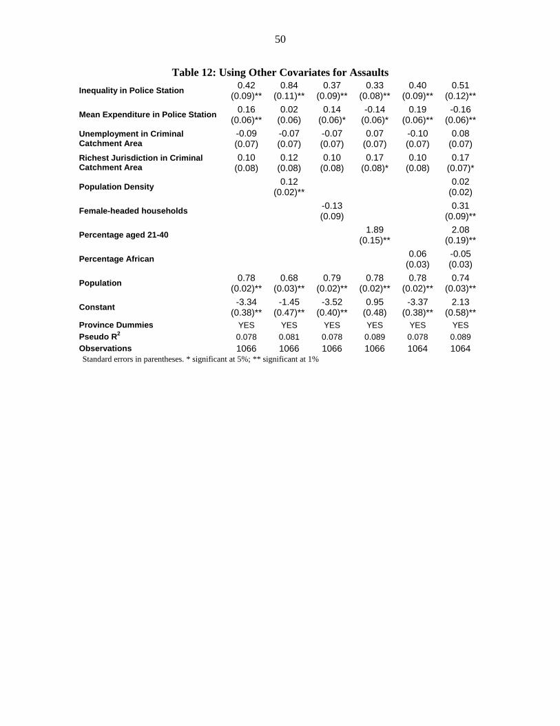
50

Table 12: Using Other Covariates for Assaults


0.84 (0.11)**

0.37 (0.09)**

0.33 (0.08)**

0.40 (0.09)**

0.51 (0.12)**


0.02 (0.06)

0.14 (0.06)*

-0.14 (0.06)*

0.19 (0.06)**

-0.16 (0.06)**


-0.09 (0.07)

-0.07 (0.07)

-0.07 (0.07)

0.07 (0.07)

-0.10 (0.07)

0.08 (0.07)


0.10 (0.08)

0.12 (0.08)

0.10 (0.08)

0.17 (0.08)*

0.10 (0.08)

0.17 (0.07)*


(0.02)**

0.02 (0.02)

Female-headed households -0.13 (0.09)

0.31

(0.09)**


(0.15)**

2.08 (0.19)**


(0.03) -0.05 (0.03)


0.68 (0.03)**

0.79 (0.02)**

0.78 (0.02)**

0.78 (0.02)**

0.74 (0.03)**

Constant -3.34 (0.38)**

-1.45 (0.47)**

-3.52 (0.40)**

0.95 (0.48)

-3.37 (0.38)**

2.13 (0.58)**


51

Table 13: Using Other Covariates for Rapes


0.87 (0.10)**

0.20 (0.09)*

0.13 (0.08)

0.24 (0.08)**

0.37 (0.10)**


0.07 (0.05)

0.23 (0.05)**

-0.02 (0.05)

0.35 (0.05)**

-0.04 (0.05)


-0.01 (0.07)

0.00 (0.06)

0.01 (0.07)

0.14 (0.06)*

-0.05 (0.07)

0.12 (0.06)*


0.04 (0.07)

0.09 (0.07)

0.04 (0.07)

0.13 (0.07)

0.03 (0.07)

0.14 (0.07)*


(0.02)**

0.05 (0.02)**

Female-headed households -0.27

(0.08)**

0.15 (0.09)


(0.13)**

1.97 (0.17)**


(0.03)** 0.03

(0.03)


0.69 (0.03)**

0.87 (0.02)**

0.82 (0.02)**

0.83 (0.02)**

0.76 (0.03)**

Constant -6.44 (0.35)**

-3.81 (0.42)**

-6.86 (0.37)**

-1.83 (0.43)**

-6.52 (0.35)**

-1.01 (0.52)


52

Table 14: Crime and Inequality using OLS


Residential Burglary Vehicle Theft Aggravated Assault Rape


1.03 (0.17)**

0.97 (0.08)**

0.76 (0.09)**

Constant -3.37 (0.14)**

-6.78 (0.21)**

-3.96 (0.09)**

-5.95 (0.11)**

Province Dummies YES YES YES YES

Adjusted-R2 0.28 0.25 0.22 0.10 Observations 1066 1066 1066 1066

Standard errors in parentheses. * significant at 5%; ** significant at 1%. Dependent variable is the log per capita crime rate. All explanatory variables are in logs. Crime rates equal to zero were replaced with the smallest value for that crime.

Table 15: Crime, Inequality and Mean Expenditure using OLS Property Crimes Violent Crimes

Residential

Burglary Vehicle Theft Aggravated Assault Rape


-0.23 (0.15)

0.93 (0.08)**

0.61 (0.10)**


1.05 (0.06)**

1.92 (0.08)**

0.06 (0.04)

0.23 (0.05)**

Constant -11.05 (0.44)**

-20.77 (0.63)**

-4.39 (0.34)**

-7.66 (0.41)**


Adjusted-R2 0.45 0.50 0.22 0.12 Observations 1066 1066 1066 1066

Standard errors in parentheses. * significant at 5%; ** significant at 1%. Dependent variable is the log per capita crime rate. All explanatory variables are in logs. Crime rates equal to zero were replaced with the smallest value for that crime.

53

Table 16: Crime, Inequality, Mean Expenditure and Unemployment using OLS



Assault Rape


-0.22 (0.15)

0.93 (0.08)**

0.61 (0.10)**


1.95 (0.10)**

0.06 (0.05)

0.24 (0.06)**


0.10 (0.13)

0.02 (0.07)

0.03 (0.08)


Constant -11.03 (0.44)**

-20.80 (0.63)**

-4.40 (0.34)**

-7.66 (0.41)**

Adjusted-R2 0.46 0.50 0.22 0.12 Observations 1066 1066 1066 1066 Standard errors in parentheses. * significant at 5%; ** significant at 1%. Dependent variable is the log per capita crime rate. All explanatory variables are in logs. Crime rates equal to zero were replaced with the smallest value for that crime.

Table 17: Crime and the Distribution of Welfare in Catchment Area using OLS



Assault Rape


-0.22 (0.15)

0.93 (0.08)**

0.61 (0.10)**


1.89 (0.10)**

0.03 (0.06)

0.25 (0.07)**


0.07 (0.13)

-0.00 (0.07)

0.03 (0.09)


0.27 (0.11)*

0.24 (0.16)

0.12 (0.09)

-0.02 (0.10)


Constant -10.70 (0.46)**

-20.51 (0.66)**

-4.25 (0.35)**

-7.68 (0.42)**


54

Table 18: Crime and Inequality between Racial Groups using OLS



Assault Rape

Within-Racial Group Inequality in Police Station

0.76 (0.23)**

1.87 (0.34)**

1.19 (0.18)**

1.48 (0.22)**

Between-Racial Group Inequality in Police Station

0.14 (0.01)**

-0.01 (0.02)

0.09 (0.01)**

0.05 (0.01)**


1.65 (0.11)**

-0.06 (0.06)

0.12 (0.07)


-0.02 (0.13)

-0.03 (0.07)

-0.04 (0.09)


0.25 (0.11)*

0.19 (0.16)

0.10 (0.09)

-0.05 (0.10)


Constant -9.62 (0.64)**

-16.31 (0.92)**

-2.63 (0.50)**

-5.33 (0.59)**


55

Table 19: Murder and Robbery Murder Armed Robbery


0.33 (0.09)**

0.16

(0.13) -0.56

(0.12)**

Mean Expenditure 0.25

(0.05)** 0.24

(0.06)**

1.20 (0.07)**

1.15 (0.07)**


0.11 (0.07)

0.12 (0.07)

0.49

(0.09)** 0.43

(0.10)**

Richest Police Station among Neighbors

0.05 (0.08)

0.05 (0.08)

-0.16 (0.11)

-0.17 (0.11)

Within-Group Inequality 0.29

(0.18)

0.14 (0.24)

Between-Group Inequality 0.03

(0.01)**

-0.06 (0.02)**


0.90 (0.02)**

0.88 (0.02)**

0.89 (0.03)**

0.88 (0.03)**

0.87 (0.03)**


-0.06 (0.11)

-0.09 (0.12)

0.16 (0.14)

0.64 (0.15)**

0.43 (0.17)*


-0.21 (0.13)

-0.20 (0.13)

-0.92 (0.21)**

-0.13 (0.20)

-0.28 (0.20)

Free State -0.62 (0.11)**

-0.46 (0.12)**

-0.43 (0.12)**

0.08 (0.17)

1.13 (0.17)**

0.90 (0.17)**

Kwazulu-Natal 0.25 (0.08)**

0.26 (0.10)*

0.21 (0.11)

1.52 (0.14)**

1.83 (0.14)**

1.73 (0.15)**

Northwest Province -0.42 (0.10)**

-0.34 (0.12)**

-0.35 (0.13)**

0.50 (0.17)**

1.28 (0.17)**

1.05 (0.18)**

Gauteng 0.33 (0.09)**

0.16 (0.10)

0.13 (0.10)

2.56 (0.15)**

2.04 (0.13)**

2.09 (0.13)**

Mpumalanga -0.27 (0.10)**

-0.27 (0.11)*

-0.29 (0.12)*

1.12 (0.17)**

1.66 (0.16)**

1.53 (0.16)**

Northern Province -1.01 (0.11)**

-0.97 (0.13)**

-0.97 (0.15)**

0.53 (0.18)**

1.02 (0.18)**

0.67 (0.21)**

Constant -5.84 (0.22)**

-7.25 (0.36)**

-6.82 (0.54)**

-6.42 (0.32)**

-14.36 (0.54)**

-13.51 (0.76)**

Pseudo R2 0.148 0.149 0.149 0.148 0.151 0.150 Observations 1066 1063 1061 1066 1063 1061 Standard errors in parentheses. * significant at 5%; ** significant at 1%. Within-Group and Between-Group Inequality refer to inequality within and between racial groups in each police station.

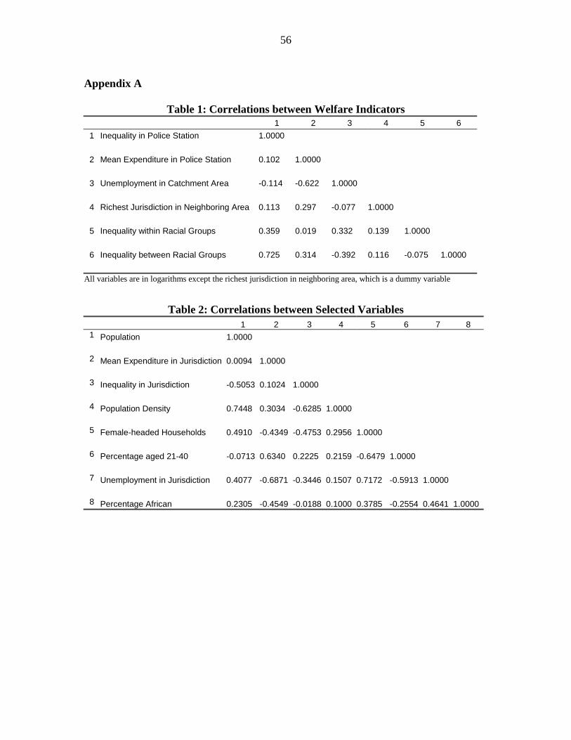
56

Appendix A

Table 1: Correlations between Welfare Indicators 1 2 3 4 5 6

1 Inequality in Police Station 1.0000

2 Mean Expenditure in Police Station 0.102 1.0000

3 Unemployment in Catchment Area -0.114 -0.622 1.0000

4 Richest Jurisdiction in Neighboring Area 0.113 0.297 -0.077 1.0000

5 Inequality within Racial Groups 0.359 0.019 0.332 0.139 1.0000

6 Inequality between Racial Groups 0.725 0.314 -0.392 0.116 -0.075 1.0000

All variables are in logarithms except the richest jurisdiction in neighboring area, which is a dummy variable

Table 2: Correlations between Selected Variables 1 2 3 4 5 6 7 8

1 Population 1.0000

2 Mean Expenditure in Jurisdiction 0.0094 1.0000

3 Inequality in Jurisdiction -0.5053 0.1024 1.0000

4 Population Density 0.7448 0.3034 -0.6285 1.0000

5 Female-headed Households 0.4910 -0.4349 -0.4753 0.2956 1.0000

6 Percentage aged 21-40 -0.0713 0.6340 0.2225 0.2159 -0.6479 1.0000

7 Unemployment in Jurisdiction 0.4077 -0.6871 -0.3446 0.1507 0.7172 -0.5913 1.0000

8 Percentage African 0.2305 -0.4549 -0.0188 0.1000 0.3785 -0.2554 0.4641 1.0000

57

Appendix B

Brief methodological description on small area estimation of welfare indicators

What follows is an overview of the methodology we employ to construct welfare

indicators for small geographical areas, such as the police station jurisdictions in South

Africa. We provide this section so that the reader is clear about the source of the welfare

measures utilized as explanatory variables in the crime regressions throughout the rest of

this paper. Please see Elbers, Lanjouw, and Lanjouw (2002) for a fuller discussion, and

Babita, Demombynes, Makhatha, and Özler (2002) for details regarding the specific

application to the South Africa data.

The basic methodology applied in linking surveys and census-type data sets is very

similar to that of synthetic estimation used in small-area geography. Prediction models are

derived for consumption or income as the endogenous variable, on the basis of the survey.

The selection of right-hand side variables is restricted to those variables that can also be

found in the census (or some other large data set). The parameter estimates are then applied

to the census data and poverty and inequality statistics derived. Simple performance tests

can be conducted which compare basic poverty or inequality statistics across the two data

sets (at representative levels for the household survey). For Ecuador, Madagascar, and

South Africa, Demombynes et al (2002) show that stratum level poverty estimates derived

from consumption measured directly in the household survey, are very similar to those

calculated on the basis of imputed household consumption in the census.

The calculation of poverty and inequality statistics using predicted income or

consumption has to take into account that each individual household income or consumption

value has been predicted and has standard errors associated with it. Elbers et al (2002) show

58

that the approach yields estimates of the incidence of poverty and of inequality that are

consistent, and that the standard errors are reasonably precise for small geographic units,

such as parroquias in Ecuador. Furthermore, a recent case study from15 demonstrates that

these estimates are precise enough to permit meaningful pair-wise comparisons across 2nd

and 3rd levels of administration.

As described above, the concept of imputing expenditures for each household in

the census is simple to grasp, yet it requires great attention to detail, especially regarding

the computation of standard errors. This also makes the exercise computationally quite

intensive. It involves constructing an association model between per capita household

expenditure and household characteristics that are common to both the census and the

household survey. After carefully constructing the variables in the exact same manner in

each data set, we estimate a regression model of logarithmic per capita household

expenditure on the other constructed variables that consist of household composition,

education, primary occupation, quality of housing, and access to services.

The basis of the approach is that per capita household expenditure for a household

h in cluster c can be explained using a set of observable characteristics. These

observable characteristics must be found as variables in both the survey and the census:16

(1) chchchch uyEy += ][lnln x .

15 See Mistiaen et al (2002). 16 The explanatory variables are observed values and thus need to have the same definitions and the same degree of accuracy across data sources. In Babita et al (2002), the criteria and approach used to select these explanatory variables are explained in detail. Finally, note that from a methodological standpoint it does not matter whether these variables are exogenous.

59

Using a linear approximation to the conditional expectation, the household’s logarithmic

per capita expenditure is modeled as

(2) chchch uy += βx 'ln .

More explicitly, we model the disturbance term as

chcchu εη +=

where cη is the cluster component and chε is the household component. This complex

error structure will not only allow for spatial autocorrelation, i.e. a “location effect” for

households in the same area, but also for heteroskedasticity in the household component

of the error. The two error components are independent of one another and uncorrelated

with observable characteristics.

The model in (2) is estimated by Generalized Least Squares using the household

survey data. The results from this first stage of the analysis are a set of estimated model

parameters, including the beta vector, an associated variance-covariance matrix, and

parameters describing the distribution of the disturbances.

To avoid forcing the parameter estimates to be the same for all areas in South

Africa, we run the first stage regressions separately for each of the 9 provinces. The

explanatory power of the nine regressions ranged from an adjusted-R2 of 0.47 (Eastern

Cape) to 0.72 (Free State), with the median adjusted-R2 equal to 0.6417.

In the second stage analysis we combine these parameter estimates based on the

survey data with household characteristics from the census data to estimate welfare

measures for subgroups of the census population. It is possible to produce these estimates

60

for any subgroups that can be identified in the census. For the purposes of this paper, we

perform the calculations at the police station jurisdiction levels.

Specifically, we combine the estimated first stage parameters with the observable

characteristics of each household in the census to generate predicted log expenditures and

relevant disturbances. We simulate a value of expenditure for each household, chy , based

on both predicted log expenditure, βx~

'ch , and the disturbance terms, cη~ and chε~ using

bootstrap methods:

(3) ( )chcchchy εη ~~~'expˆ ++= βx .

For each household, the two disturbance terms are drawn from distributions

described by parameters estimated in the first stage18. The beta coefficients, β~ , are drawn

from the multivariate normal distribution described by the first stage beta estimates and

their associated variance-covariance matrix. We then use the full set of simulated chy

values to calculate expected values of the average expenditure, poverty, and inequality

measures for the two spatial subgroups described above.

We repeat this procedure 100 times, drawing a new set of beta coefficients and

disturbances for each set of simulations. For each subgroup, we take the mean and

standard deviation of the welfare indicators over all 100 simulations. For any given

location, these means constitute the point estimates of the welfare indicators, while the

standard deviations are the standard errors of these estimates.

17 The R-squared values that we report are from OLS models. We do this to give our readers a sense of the explanatory power of our regression models, as there is no precise counterpart to R-squared in a GLS model. See Greene (1997), p. 508 for details. 18 Please note that these errors are not necessarily drawn from a normal distribution. For details, please refer to Babita et al (2002).

61

There are two principal sources of error in the welfare measure estimates

produced by this method.19 The first component, referred to as model error in Elbers et

al (2002), is due to the fact that the parameters from the first-stage model in equation (2)

are estimated. The second component, described as idiosyncratic error, is associated

with the disturbance term in the same model, which implies that households’ actual

expenditures deviate from their expected values. While population size in a location does

not affect the model error, the idiosyncratic error increases as the number of households

in a target population decreases.

19 A third potential source of error is associated with computation methods. Elbers et al (2002) found this component to be negligible with a sufficiently high number of simulation draws.

Crime and Welfare in South Africa 020902 - Williams … and... · 2002-09-07 · Crime and Local...

Documents

Transcript of Crime and Welfare in South Africa 020902 - Williams … and... · 2002-09-07 · Crime and Local...