CREEP MODELING OF WOOD USING TIME-TEMPERATURE ...

CREEP MODELING OF WOOD USING TIME-TEMPERATURE SUPERPOSITION

Sandhya Samarasinghe Lecturer

Department of Natural Resources Engineering Lincoln University

Canterbury, New Zealand

Joseph R. Loferski Associate Professor

Department of Wood Science and Forest Products

and

Siegfried M. Holzer Professor

Department of Civil Engineering Virginia Polytechnic Institute and State University

Blacksburg, VA 2406 1

(Received September 1992)

ABSTRACT

The time-temperature superposition principle was used to develop long-term compression creep and recovery models for southern pine exposed to constant environmental conditions using short- term data. Creep (1 7-hour) and recovery (40-hour) data were obtained at constant temperature levels ranging from 70 F to 150 F and constant equilibrium moisture content (EMC) of 9%. The data were plotted against log-time, and the resultant curve segments were shifted along the log-time axis with respect to the curve for ambient conditions to construct a master curve applicable to ambient conditions (70 F, 9% EMC) and a longer time period. The master curves were represented by power functions, and they predicted up to 6.4 years of creep and 5.8 years of recovery response. The validity of the master curves for predicting creep of wood exposed to the normal interior environment in buildings was tested by conducting ten-month creep tests in the laboratory. The fluctuating environment caused geometry changes in the surface of the specimens affecting the collected long-term data. Therefore, a good comparison between the master curves and the long-term data was not possible.

Keywords: Time-temperature superposition, long-term creep modeling, accelerated creep, master curves, activation energy.

INTRODUCTION

Wood is a competitive construction material due to technological advances in the development of engineered wood products. Glu- lam space trusses and frames, such as domes, are competing with metallic structures that had traditionally dominated the market (Holzer et al. 1989). However, Hayman (198 1) demon- strates that shallow arches can experience snap- through buckling due to creep magnified by the P-A effect, also known as geometric non-

linearity. For example, creep deflection in a shallow arch or dome causes shortening of its members, leading to a shallower arch/dome configuration. This results in increased member stresses causing magnified creep deflec- tions, which in turn increase member stresses. This feedback loop process (P-A effect) can continue until the arch/dome becomes unsta- ble and snaps-through to an inverted position. The P-A effect can also cause a loss of load carrying capacity in crooked columns (Itani et al. 1986).

Wood and Fiber Science. 26(1), 1994, pp. 122-130 O 1994 by the Society of Wood Science and Technology

Samarasinghe et a/. -CREEP MODELING US1 NG TIME-TEMPERATURE SUPERPOSITION 123

The current design practices recommend constant factors to account for creep deflection in wood structures. However, these factors may not be sufficient to guarantee the long-term safety of innovative wood structures, such as shallow arches and domes, where creep can be significant. However, there are no established methods to predict creep effects on the safety and serviceability of wood structures. Al- though few relatively long-term (10-year) em- pirical bending creep models have been developed (Clausser 1959; Gressel 1984), models representing material behavior, such as pure tension, compression, and shear creep models, are more suitable for creep analysis based on numerical methods, such as the finite-element method which is well established for creep analysis of metallic structures (Kraus 1980; Holzer et al. 1989). However, the existing creep models for wood in tension, compression, and shear apply to short time periods only (Sa- marasinghe 199 1 ; Schniewind 1968).

The time-temperature superposition principle (TTSP) is highly developed for polymers for predicting long-term response from short- term data (Aklonis and MacKnight 1983). The objective of this study was to test the validity of the TTSP to develop long-term creep and recovery models for kiln-dried southern pine Pinus spp.) loaded in compression parallel-to- grain and exposed to constant ambient environmental conditions ( ~ 7 0 F, ~ 9 % EMC).

TIME-TEMPERATURE SUPERPOSITION

PRINCIPLE (TTSP)

The TTSP states that a property measured over a short time at a higher temperature is equivalent to the property measured over a long time at a lower temperature (Aklonis and MacKnight 1983; Rosen 197 1). The application of TTSP to the relaxation modulus of a polymer is illustrated in Fig. 1 (Rosen 197 1). Short-term experimental data for successively increasing temperature levels (accelerated data) are plotted against log-time as shown in Fig. l(a). The curve segments for temperatures above the reference temperature are shifted right, and those below the reference temper-

w-tb.M FIG. 1. Process of master curve formation: (a) accel-

erated data, (b) master curve, (c) shift factor vs. temperature (Rosen 197 1).

ature are shifted left along the log-time axis with respect to the reference temperature curve until each curve smoothly joins to form a master curve as shown in Fig. l(b). The master curve is applicable to the reference temperature and a longer time period. The horizontal displacement of each curve is called the shift factor, log a,; and the relationship between log a, and temperature is shown in Fig. I(c).

For reference temperatures below the glass transition temperature (T,), the shift factor is related to the absolute temperature (T) by an activation energy (AH) through the Arrhenius equation (Aklonis and Macknight 1983)

R log a, AH = 2.030

11T - llTg (1)

where R is the universal gas constant. Schaffer (1978) indicates that the TTSP may be applicable to wood over narrow temperature ranges. Schaffer (1 978) also reports that Yamada et al. observed a good compliance with TTSP for the relaxation modulus of wet beech. Salmkn (1984) successfully applied TTSP to the dynamic mechanical properties of water-saturated Norway spruce (Picea abies). Kelly et al. (1987) applied TTSP to Sitka spruce (Picea sitchensis Bong Carr.) plasticized with ethyl formamide.

To achieve the objective stated in this paper, two types of creep tests were conducted: ( I ) short-term accelerated creep tests to develop TTSP based long-term creep models, and (2) long-term creep tests to validate TTSP based on long-term creep models. Accordingly, Sec-

124 WOOD AND FIBER SCIENCE, JANUARY 1994, V. 26(1)

TABLE I . Material properties of accelerated test specimens.

Moisture Young's Ultimate Specimen content Spec~fic modulus comp. stress

No. (%) gravlty* ( loh psi) (psi)

* Spec~fic gravlty 1s based on oven-dry we~ght and volume.

tion I is devoted to the development of long- term creep and recovery models based on TTSP using short-term accelerated data, and Section I1 deals with the validation of TTSP based long-term creep models with long-term experimental creep data.

I. DEVELOPMENT OF LONG-TERM CREEP

AND RECOVERY CURVES USING TTSP

In this section, long-term creep and recovery models applicable to constant ambient environmental conditions (70 F, 9% EMC) are developed from short-term accelerated data using TTSP.

Short-term accelerated creep tests

Specimens and materialproperties. -All the specimens were prepared from kiln-dried southern pine conditioned to 9% EMC. For each short-term accelerated creep test specimen, there was a corresponding long-term creep test specimen (see Section 11) end-matched with it. Additionally, a dummy specimen, similar in dimensions to creep test specimens, was used alongside of each creep test specimen during experiments to minimize the effects of factors other than creep on the measured strain as discussed later. Thus, the preparation of a sin- gle pair of end-matched short-term and long- term test specimens involved the preparation of two additional dummy specimens (total of

four) as follows: Four end-matched '/2-in. x

'/2-in. x 3-in. specimens were prepared from clear, straight-grained material, and the first two specimens were used as a matched pair of short-term and long-term creep test specimens (active specimens), and the other two were used as unloaded (dummy) specimens. Similarly, a total of 1 1 short-term test specimens, 11 long- term test specimens were prepared along with 22 dummy specimens to be used with creep test specimens. The ASTM D 143 compression tests were conducted on 1 -in. x 1 -in. x 4-in. specimens, end-matched with the creep test specimens, to determine material properties. Table 1 shows the Young's modulus (E), ultimate compressive stress, moisture content, and specific gravity of the eleven specimens used in the accelerated tests.

Load level, test environment, strain measurement. -A constant stress of 1,675 psi (370 pounds) equivalent to 16% of the experimen- tally determined mean ultimate stress was applied to all the test specimens. Since the creep response of structures is in the glassy region, the maximum temperature for the creep tests should be below T, of southern pine; tests done with a dynamic mechanical thermal analyzer (DMTA) indicated that the Tg of the test material was 260 F. Creep tests were conducted at temperature levels ranging from 70 F to 150 F with eight successive steps of 10 F. The relative humidity of the accelerated test environment was adjusted at each temperature so that the EMC was maintained at 9% according to the published psychrometric charts. Heated air conditioned at each specified temperature and humidity was supplied by a laboratory environmental chamber.

The compressive strain in the accelerated tests was measured by strain gages bonded on two opposite sides of each active and dummy specimen and connected in a Wheatstone bridge circuit as shown in Fig. 2 (Samarasinghe 199 1). Strain gages used in this study were self- temperature compensating constantan alloy foil strain gages mounted on a plastic backing. The gages were bonded to the wood surface using an epoxy adhesive, AE-10, provided by the

Samarasinghe et al. -CREEP MODELING USING TIME-TEMPERATURE SUPERPOSITION 125

active specimen

dummy specimen

\ lead wires

FIG. 2. Creep strain measurement: (a) active and dummy specimens and gages, (b) Wheatstone bridge circuit.

strain gage manufacturer, and the bonded gages were covered with a moisture protective coating. The gage arrangement shown in Fig. 2 was designed to measure pure compressive strain and eliminate bending and temperature effects (Perry and Lissner 1962). When bonded to steel, self-temperature compensating gages automatically compensate for the effects of the sensitivity of the gages and lead wires to temperature; however, they can be less effective on wood due to low thermal conductivity of wood, and can sense a temperature-induced apparent strain. Bending effects are due to possible load eccentricity and/or imperfect specimen geometry. The creep strain was read by a data acquisition systemon a portable IBM; PC.

Short-term accelerated compression test apparatus. -The short-term accelerated tests were conducted in an insulated test chamber. A compression test fixture with a calibrated lever arm producing a lever advantage of 1:20 was developed, and three such test fixtures were assembled in the test chamber as shown in Fig. 3. Spherical seats placed underneath the specimens minimized the load eccentricity. Five

ture transmitter were used to measure the temperature inside the chamber.

Short-term accelerated test procedure. -In short-term accelerated creep tests, creep was accelerated by testing the same specimen at successively higher temperature levels for 17 hours as follows: Three active specimens were placed in the test fixtures and the corresponding dummy specimens were located near each active specimen (Fig. 3). Three moisture monitoring specimens, cut from the same location of the boards from which active and dummy specimens were made, were coated with a

thermometers and a humidity and tempera- FIG. 3. Short-term accelerated test apparatus.

WOOD A N D FIBER SCIENCE, JANUARY 1994, V. 26(1)

FIG. 4. Short-term accelerated test curves: (a) creep, (b) recovery.

moisture protective coating and placed near the test fixtures to determine the moisture change in the test specimens during the tests. The creep test procedure was started by con- ditioning the specimens at ambient temperature and relative humidity (70 F, 49% RH) for 24 hours. The loads were applied and the creep response [Wheatstone bridge output (E,) in Fig. 2(b)] was recorded for 17 hours, and then the loads were removed and 40-hour recovery data were collected. Next, the temperature and relative humidity were raised to the next higher level (80 F, 49% RH), and the unloaded specimens were conditioned until the specimens reached equilibrium under new temperature and humidity conditions and the recovery from the previous test was complete as evidenced by the bridge output voltage. The

loads were applied and the data collection was repeated as in the previous step. This procedure was repeated in 10 F steps up to the highest test condition (1 50 F, 6 1 % RH or 140 F, 59% RH). At the highest temperature level, creep period for various specimens ranged from three to ten days, and the recovery period equalled the creep period.

After the recovery test at the highest temperature was completed, the moisture monitoring specimens were weighed. Then another three pairs of active an dummy specimens were located in the test apparatus, and the whole test procedure was repeated until all the specimens had been tested.

Short-term accelerated creep data and master curves

Short-term accelerated creep data. -The creep and recovery strains in the specimens were computed from the bridge output voltage. Creep and recoverable compliances ( 1 /modulus) at each temperature were plotted against log-time (logarithm to the base 10) as shown in Fig. 4(a) and 4(b) for a typical specimen. The data for 80 F overlapped with the data for 70 F; therefore, curves for 80 F were removed from the data sets. Figures 4(a) and 4(b) indicate that the rates of change of creep and recovery increase with temperature. Moisture monitoring tests did not indicate any moisture change within the test specimens during the tests.

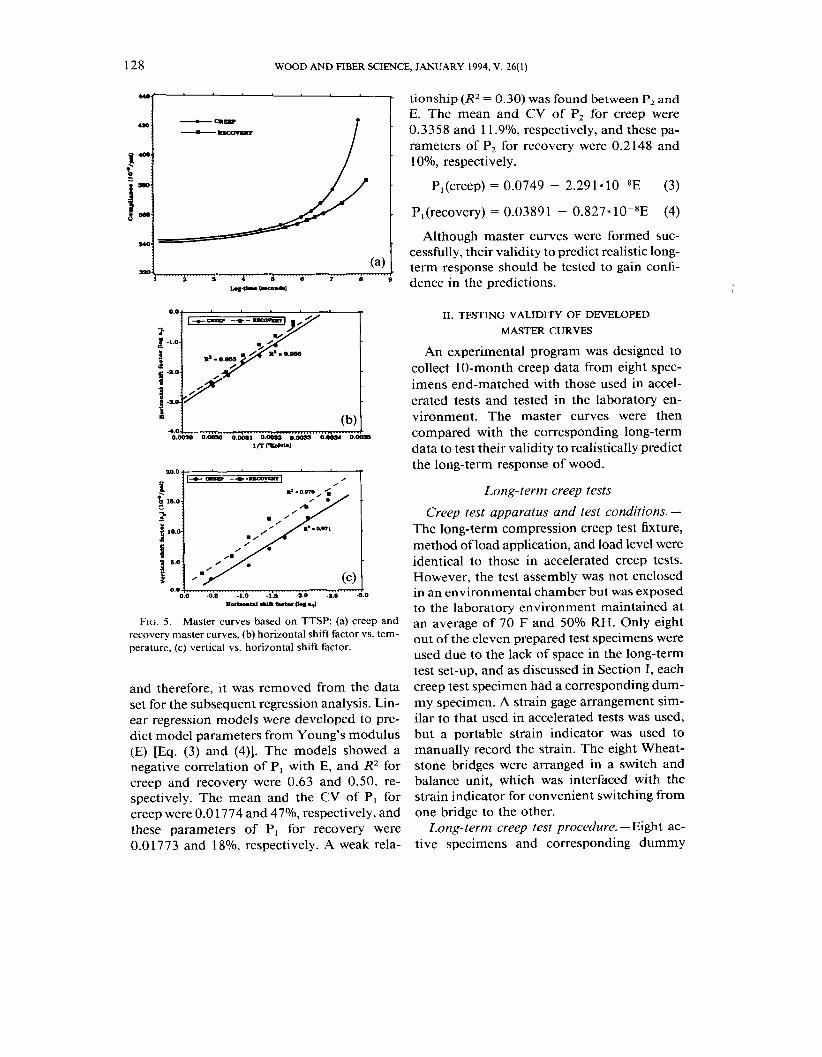
Formation of master curves. -Creep and recovery compliance master curves, applicable to 70 F, were formed for each of the eleven specimens using the corresponding sets of short-term creep and recovery data. Creep and recovery master curves developed from the curves shown in Figs. 4(a) and 4(b) for a typical specimen are shown in Fig. 5(a). Master curves of Fig. 5(a) were formed by successive joining of creep (or recovery) curves of Fig. 4(a) [or 4(b)] in regions where the slopes were equal by horizontal shifting and by a slight amount of vertical shifting to account for volume change. The points in curves of Fig. 5(a) represent where the curves of Fig. 4(a) [or 4(b)] are joined, and


TABLE 2. Master curves, model parameters, and activation energy for creep and recovery.

Cnep master curve Recovery master curve

Rel. Rel. Speci- Young's predic- creep AH Predic- recovery AH men modulus tlon a m p . tion comp. No. (10" psi) (years) (%) PI p2 PI PZ

a major portion of each curve overlapped with the corresponding master curve. Similar curves were developed from the other ten sets of data.

Generally, for all the eleven specimens, the short-term curve segments joined well to form master curves. Creep and recovery curves shown in Fig. 5(a) extend over a period of 7.9 x 1 O6 seconds or 2.55 years, and 8.15 x lo6 seconds or 4.54 years, respectively. The master curve prediction and relative creep and recovery compliances (i.e., the ratio of maximum creep or recovery compliance to elastic compliance) for all the specimens are summarized in Table 2. The table shows that the master curves predict the creep response up to 6.4 years and recovery response up to 5.8 years. This extension varied with the nature of the short-term curves.

The master curves for a typical specimen as shown in Fig. 5(a) indicate that the TTSP can be used to develop long-term creep and recovery curves. Since the predicted long-term response was within the glassy response region of wood, the shift factor should follow the Ar- rhenius formulation expressed by Eq. (I), which states that the relationship between log a, and 1/T is linear. The linear regression analyses showed a strong linear relationship between log a, and 1/T, with the coefficient of deter- mination (R2) for all the data sets ranging from 0.889 to 0.995. This relationship for the creep and recovery master curves shown in Fig. 5(a)

is shown in Fig. 5(b). These results indicate that the Arrhenius formulation was satisfied, and therefore master curve formation was suc- cessful.

The relationship between log a, and 1 /T was also used to compute the activation energy (AH) for creep and recovery using Eq. (I), and the AH values are presented in Table 2. The means and the coefficients of variation (CV) of the activation energy for creep (27.10 KCal/mole, 2 1.1%) and recovery (28.18 KCaVmole, 18.8%) were quite close. Salmin (1 984) states that AH varies from about 9.5 KCal/mole and up- wards, depending on the T, of the material. The linear relationship between the vertical shift factor (a,) and log a,, as shown in Fig. 5(c), suggests that there are no changes in the activation mechanism of creep and recovery within the test temperature range.

The creep and recovery master curves were represented by

where D,,/Do is the relative creep (or recovery) compliance, Dc, is the creep (or recovery) compliance (l/psi), Do is the elastic compliance (l/psi), P, and P2 are estimated parameters, and t is the time (hours). The model parameters are shown in Table 2.

Scatter plots revealed that the value of 0.1868 for P, for specimen number 8 was an outlier


- tionship (R2 = 0.30) was found between P, and E. The mean and CV of P, for creep were 0.3358 and 1 1.9%, respectively, and these parameters of P, for recovery were 0.2148 and 1 OO/o, respectively.

P, (creep) = 0.0749 - 2.29 1 * 1OP8E (3)

- P,(recovery) = 0.03891 - 0.827; 1OP8E (4)

Although master curves were formed successfully, their validity to predict realistic long-

(a).t term response should be tested to gain confi- ' dence in the predictions.

FIG. 5. Master curves based on TTSP: (a) creep and recovery master curves, (b) horizontal shift factor vs. temperature, (c) vertical vs. horizontal shift factor.

and therefore, it was removed from the data set for the subsequent regression analysis. Lin- ear regression models were developed to predict model parameters from Young's modulus (E) [Eq. (3) and (4)]. The models showed a negative correlation of P, with E, and R2 for creep and recovery were 0.63 and 0.50, respectively. The mean and the CV of PI for creep were 0.0 1774 and 47%, respectively, and these parameters of PI for recovery were 0.0 1773 and 18%, respectively. A weak rela-

11. TESTING VALIDlTY OF DEVELOPED

MASTER CURVES

An experimental program was designed to collect 10-month creep data from eight specimens end-matched with those used in accelerated tests and tested in the laboratory environment. The master curves were then compared with the corresponding long-term data to test their validity to realistically predict the long-term response of wood.

Long-term creep tests

Creep test apparatus and test conditions. - The long-term compression creep test fixture, method of load application, and load level were identical to those in accelerated creep tests. However, the test assembly was not enclosed in an environmental chamber but was exposed to the laboratory environment maintained at an average of 70 F and 50% RH. Only eight out of the eleven prepared test specimens were used due to the lack of space in the long-term test set-up, and as discussed in Section I, each creep test specimen had a corresponding dummy specimen. A strain gage arrangement similar to that used in accelerated tests was used, but a portable strain indicator was used to manually record the strain. The eight Wheat- stone bridges were arranged in a switch and balance unit, which was interfaced with the strain indicator for convenient switching from one bridge to the other.

Long-term creep test procedure. -Eight active specimens and corresponding dummy


specimens were placed in the test fixtures. \ Moisture monitoring specimens were also located near the test specimens. The loads were applied to the active specimens, and the creep strain was recorded for ten months. The first step in measuring strain with strain gages is to balance the Wheatstone bridge. This position is called the null balance point or zero reference point with respect to which subsequent strains are measured after loading a specimen. However, it has been observed that the zero

I reference point can change with time in long- term strain measurements (Perry and Lissner 1962). This phenomenon, called zero drift, can lead to slightly modified strains read by the strain indicator. The zero drift can be moni- tored by comparing the strain reading corresponding to the reversed position of gages in the Wheatstone bridge with that corresponding to the normal gage positions, and the two readings must be identical in the absence of the zero drift. This procedure was repeated at each time a strain was recorded and no zero drift was encountered.

Long-term data and master curve validation

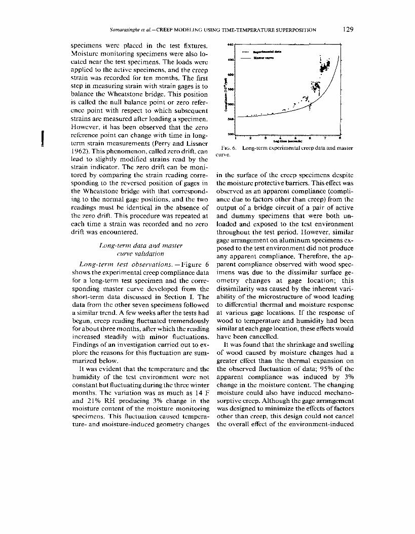
Long-term test observations. -Figure 6 shows the experimental creep compliance data for a long-term test specimen and the corresponding master curve developed from the short-term data discussed in Section I. The data from the other seven specimens followed a similar trend. A few weeks after the tests had begun, creep reading fluctuated tremendously for about three months, after which the reading increased steadily with minor fluctuations. Findings of an investigation carried out to ex- plore the reasons for this fluctuation are summarized below.

It was evident that the temperature and the humidity of the test environment were not constant but fluctuating during the three winter months. The variation was as much as 14 F and 21% RH producing 3% change in the moisture content of the moisture monitoring specimens. This fluctuation caused temperature- and moisture-induced geometry changes

IrEtb.(rcol..)

FIG. 6 . Long-term experimental creep data and master curve.

in the surface of the creep specimens despite the moisture protective barriers. This effect was observed as an apparent compliance (compliance due to factors other than creep) from the output of a bridge circuit of a pair of active and dummy specimens that were both unloaded and exposed to the test environment throughout the test period. However, similar gage arrangement on aluminum specimens exposed to the test environment did not produce any apparent compliance. Therefore, the apparent compliance observed with wood specimens was due to the dissimilar surface geometry changes at gage location; this dissimilarity was caused by the inherent vari- ability of the microstructure of wood leading to differential thermal and moisture response at various gage locations. If the response of wood to temperature and humidity had been similar at each gage location, these effects would have been cancelled.

It was found that the shrinkage and swelling of wood caused by moisture changes had a greater effect than the thermal expansion on the observed fluctuation of data; 95% of the apparent compliance was induced by 3% change in the moisture content. The changing moisture could also have induced mechano- sorptive creep. Although the gage arrangement was designed to minimize the effects of factors other than creep, this design could not cancel the overall effect of the environment-induced


localized geometry changes. Although at- tempts were made to eliminate these effects from collected data, considerable improve- ment was not attained.

Figure 6 shows that the creep data and master curves agreed well in the first few weeks when there was little environmental fluctuation. Later, the master curves deviated from the data due to the changing environment. Al- though master curves followed the trend of the data, the creep response predicted by master curves was consistently lower than the corresponding long-term creep data. At the end of the ten months, a discrepancy of 28% to 50% was found between the predicted and the experimental creep compliance (D,,) for the eight specimens. Schaffer (1 972) states that during cycling between wet and dry moisture conditions, the deflection of wood increases or de- creases with the change. However, total rate of creep has proved to be substantially greater than that under constant moisture conditions. His statement verifies the fact observed by other investigators (Schniewind 1968) that mechano-sorptive (M-S) creep increases under cyclic moisture conditions, but the effect of M-S creep under very slowly and slightly vary- ing moisture conditions over a period of months, as observed in this study, on the measured strain is uncertain.

CONCLUSIONS

The time-temperature superposition principle can be used to develop master curves for predicting long-term response of kiln-dried southern pine loaded in compression parallel- to-grain and exposed to constant environmental conditions (70 F, 9% EMC). Developed master curves predicted up to 6.4 years ofcreep and 5.8 years of recovery response. The activation energy of creep and recovery of wood within the temperature range of 70 F to 150 F was approximately 28 KCal/mole. In this temperature range, there was no change in the activation mechanism of creep and recovery. The validation of the developed master curves was not possible due to the effect of changing en-

vironment on the long-term strain measurements. For a proper validation, the long-term tests must be conducted either in a constant environment or with a better moisture protective barrier on the specimens.

REFERENCES

Aklonis, J. J., and W. J. MacKnight. 1983. Introduction to polymer viscoelasticity, 2nd ed. John Wiley and Sons, New York, NY.

Clauser, W. S. 1959. Creep of small wood beams under constant bending load. USDA Forest Service Report No. 21 50, Forest Products Lab, Madison, WI.

Gressel, P. 1984. Prediction of long-term deformation behavior from short-term creep experiments. Holz Roh- Werkst. 42:293-301.

Hayman, B. 198 1. Creep buckling-A general view of the phenomenon. Pages 289-307 in A. R. S. Ponter and D. R. Hayhurst, eds. Proceedings of the Third IUTAM Symposium on Creep in Structures. Springer-Verlag, New York, NY.

Holzer, S. M., D. A. Dillard, and J. R. Loferski. 1989. A review of creep in wood: Concepts relevant to long- term behavior predictions for wood structures. Wood Fiber Sci. 2 1(4):376-392.

Itani, R. Y., M. C. Griffith, and R. J. Hoyle, Jr. 1986. The effect of creep on long wood column design and performance. J. Struct. Eng. 1 12(5): 1097-1 1 14.

Kelly, S. S., T. G. Rilas, and W. G. Glasser. 1987. Re- laxation behavior of amorphous components of wood. J. Mater. Sci. 22:617-625.

Kraus, H. 1980. Creep analysis. John Wiley and Sons, Inc., New York, NY.

Perry, C. C., and H. R. Lissner. 1962. The strain gage primer, 2nd ed. McGraw-Hill, New York, NY. Pp. 62- 73.

Rosen, S. L. 197 1. Fundamental principles of polymeric materials for practising engineers. Barnes and Noble, Inc., New York, NY.

Salmtn, L. 1984. Viscoelastic properties of in situ lignin under water saturated conditions. J. Mater. Sci. 19:3090- 3096.

Samarasinghe Gamalath, S. 199 1. Long-term creep modeling of wood using time temperature superposition principle. Ph.D. dissertation, Virginia Tech, Blacksburg, VA.

Schaffer, E. L. 1972. Modelling the creep of wood in a changing moisture environment. Wood Fiber 3(4):232- 235.

-. 1978. Influence of heat on the longitudinal creep of dry Douglas-fir. Pages 20-52 in Proceedings of the Symposium on Structural Use of Wood in Adverse En- vironments.

Schniewind, A. P. 1968. Recent progress in the study of the rheology of wood. Wood Sci. Technol. 2: 188-206.

CREEP MODELING OF WOOD USING TIME-TEMPERATURE ...

Documents

Transcript of CREEP MODELING OF WOOD USING TIME-TEMPERATURE ...