Credit matrics report

INVESTX PLC

Portfolio Risk Report Credit Metrics analysis on bonds’ credit risk and portfolios values

M.Zhang

3/7/2015

Mz96 Credit Metrics Report INVESTX PLC

1

Spreadsheet in Excel Page in Report

Overview

P1

Method

"Data Analysis", "Portfolio 1", "Portfolio 2"

P2-4

Results "Comparison" P5-7

Recommendation

P8

Limitations P9-10

Overview

This report analyses two bond portfolios’ credit risk with Credit Metrics methodology, which

considers how each bond’s credit rating changes given the correlation between them. So we

can do simulations and see the effect of upgrading/downgrading of bonds on the whole

portfolio’s value in one year and the credit risk is quantified by calculating Value at Risk for

the portfolio.

There are 4 states for the bonds: A rated, B rated, C rated and Default.

Nine bonds are available for investment: 6 B rated bonds (from companies: R, S, T, U, V, W)

and 3 C rated bonds (from companies: X, Y, Z) with 10 years’ term and 5% annual coupon.

Our client wishes to invest in B rated bonds only for his portfolio as he thinks it is safer.

However, considering the correlations between these bonds, there may be potential big losses

occurring. Therefore, this report looks at the following 2 portfolios:

A portfolio of 6 B rated bonds in same industry (R, S, T, U, V, W)

A portfolio of 3 B rated bonds in same industry (R, S, T) and 3 C rated bonds in

different industries (X, Y, Z)

Being in the same industry implies higher correlation between one bond to another.

By simulating portfolio values in one year’s time, we analyse the distribution pattern and

99.5% VaR for the 2 portfolios and make a recommendation about which portfolio is safer to

invest in.


2

Method

Credit Metrics model assesses credit risk due to changes of credit rating of bonds in a

portfolio, e.g. downgrading and upgrading’s effect on credit quality. By simulating different

scenarios considering the correlation between bonds, we can obtain the VaR for the portfolio

in one year.

Steps taken:

Obtain Covariance Matrix and Cholesky Matrix for bonds in the portfolio

Simulate multivariate Normal random variables using Cholesky Matrix

Return the simulated values back to the according credit rating states using transition

matrix

Calculate the values for a bond in each credit rating state

Obtain the simulated portfolio values in one year’s time

Obtain VaR 99.5% for the simulations for each portfolio

Correlation between the bonds in the portfolio is obtained by analysing the equity returns for

the companies for the past 3 years.

To do this, we first need to find the Covariance Matrix as seen in ‘Data Analysis’ spreadsheet.

Then the Cholesky Matrix( C ) is obtained from the Covariance Matrix ( ∑ ) by performing

Cholesky decomposition1 to the Covariance Matrix.

The result is checked by multiplying Cholesky Matrix with its transpose to fit equation:

CC’=∑

Cholesky Matrix allows us to generate multivariate Normal random variables xi with same

correlation as the equity returns between the companies, which we assume to represent the

bonds’ correlations in the portfolio.

The values in Excel is copied and pasted values for illustration. The first 10 rows contain

formula used, which can be easily reproduced if more simulations are needed. Then we

multiply the standard Normal random variables by transpose of Cholesky Matrix.

These correlated random variables would then be returned back to the credit ratings.

Since each simulation trial contains variables xi from standard Normal distribution with same

correlation as the bonds, it determines the new ratings in one year for each bond. Given the

Transition Matrix, we can return xi to the credit rating it belongs to in one year’s time by

inversing the cumulative transition probability with standard Normal function to set the

boundary for categorising the simulated values.

1 See Paul Sweeting- Enterprise Risk Management Formula 10.97


3

The following diagrams show how the simulated results can be categorised into four states:

A rated, B rated, C rated, or Default for a bond starts as B rated and C rated respectively.

We can see a B rated bond has largest probability to remain B rated.

-3 -2 -1 0 1 2 3

B Rated Bond

Bond remains B rated

A C Default

1.47-1.126 -1.881

If xi falls below -1.881

If xi falls between -1.881 and -1.126

If xi falls between -1.126 and 1.476 If xi is

above 1.476

-3 -2 -1 0 1 2 3

C Rated Bond

Bond remains C rated

A Default B

1.641.036 -1.036

If xi falls below -1.036

If xi falls between -1.036 and 1.036

If xi falls between -1.036 and 1.644

If xi is above 1.644


4

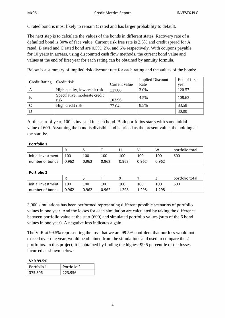
C rated bond is most likely to remain C rated and has larger probability to default.

The next step is to calculate the values of the bonds in different states. Recovery rate of a

defaulted bond is 30% of face value. Current risk free rate is 2.5% and credit spread for A

rated, B rated and C rated bond are 0.5%, 2%, and 6% respectively. With coupons payable

for 10 years in arrears, using discounted cash flow methods, the current bond value and

values at the end of first year for each rating can be obtained by annuity formula.

Below is a summary of implied risk discount rate for each rating and the values of the bonds:

Credit Rating Credit risk Current value

Implied Discount

Rate

End of first

year

A High quality, low credit risk 117.06 3.0% 120.57

B Speculative, moderate credit

risk 103.96 4.5% 108.63

C High credit risk 77.04 8.5% 83.58

D 30.00

At the start of year, 100 is invested in each bond. Both portfolios starts with same initial

value of 600. Assuming the bond is divisible and is priced as the present value, the holding at

the start is:

Portfolio 1

R S T U V W portfolio total

initial investment 100 100 100 100 100 100 600

number of bonds 0.962 0.962 0.962 0.962 0.962 0.962

Portfolio 2

R S T X Y Z portfolio total

initial investment 100 100 100 100 100 100 600

number of bonds 0.962 0.962 0.962 1.298 1.298 1.298

3,000 simulations has been performed representing different possible scenarios of portfolio

values in one year. And the losses for each simulation are calculated by taking the difference

between portfolio value at the start (600) and simulated portfolio values (sum of the 6 bond

values in one year). A negative loss indicates a gain.

The VaR at 99.5% representing the loss that we are 99.5% confident that our loss would not

exceed over one year, would be obtained from the simulations and used to compare the 2

portfolios. In this project, it is obtained by finding the highest 99.5 percentile of the losses

incurred as shown below:

VaR 99.5%

Portfolio 1 Portfolio 2

375.306 223.956


5

This means, for Portfolio 1, 99.5% of the time the loss wouldn’t exceed 375.306. For

Portfolio 2, 99.5% of the time the loss wouldn’t exceed 223.956. This result indicates that,

Portfolio 1 has a higher potential loss than Portfolio 2.


6

Results

Below is a summary statistics of the results:

Portfolio 1 Portfolio 2

Average Loss -4.39 -12.57

Average Portfolio Value 604.39 612.57

Variance 5237.32 4336.05

Max Loss 426.85 327.04

Max Gain 95.90 171.01

VaR 99.5% 375.31 223.96

Even though the average credit rating for Portfolio 1 is higher, the results show that Portfolio

2 generates a higher average return.

Also, Portfolio 2 has a lower variance, this means the portfolio values are less volatile than

Portfolio 1. The 99.5% Value at Risk for Portfolio 2 is much lower, this means at given

confidence level, the loss from Portfolio 2 is capped at a much lower level than Portfolio 1 in

one year’s time.

This is because Portfolio 2 contains 3 C rated bonds that has low correlation to each other and

to the 3 B rated bonds. The low correlation means that the portfolio is more diversified. So

when one specific market is bad, bond values would not drop together and create huge losses.

Below is a histogram of Portfolio 1:

We can see that in most case (57%) we would have a gain of 20, this is because the bonds are

relatively highly correlated, they tend to behave the same way as each other, i.e. if one bond

stays in B rating, the others are likely to stay in B rating, which causes the leptokurtic shape.

0

200

400

600

800

1000

1200

1400

1600

1800

-10

0

-80

-60

-40

-20 0

20

40

60

80

10

0

12

0

14

0

16

0

18

0

20

0

22

0

24

0

26

0

28

0

30

0

32

0

34

0

36

0

38

0

40

0

42

0

mo

re

Loss

Portfolio 1 Histogram


7

However, if one bond performs badly, the others are likely to behave the same way, which

causes the potential huge loss (greatest loss lies beyond 420 for a probability of 0.43%) in the

tail area. The tail is long and fat, which means there is a chance of catastrophic risk.

Below is a histogram for Portfolio 2:

Values for portfolio 2 is spreat more evenly. With four peaks at -70, -30, 40, and 110, these

may be caused by the 3 correlated B rated bonds (R, S, T) behaving in similar ways. But the

effect is offset by the 3 less correlated bonds (X, Y, Z).

It has a positive skew showing a chance of general trend of gain. The lagest loss is around

330 with a probability of 0.07% which is a much lower change for a lower loss compared to

Portfolio 1.

0

100

200

300

400

500

600

700

800

-18

0

-16

0

-14

0

-12

0

-10

0

-80

-60

-40

-20 0

20

40

60

80

10

0

12

0

14

0

16

0

18

0

20

0

22

0

24

0

26

0

28

0

30

0

32

0

Mo

re

Loss

Portfolio 2 Histogram


8

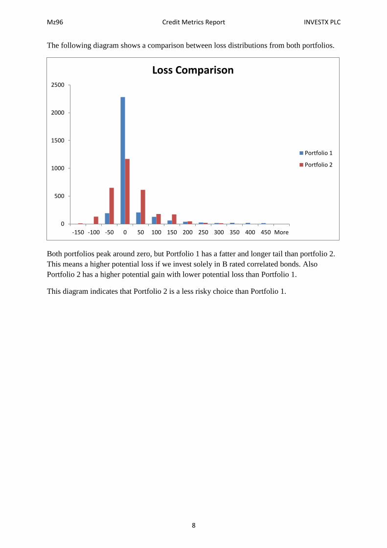
The following diagram shows a comparison between loss distributions from both portfolios.

Both portfolios peak around zero, but Portfolio 1 has a fatter and longer tail than portfolio 2.

This means a higher potential loss if we invest solely in B rated correlated bonds. Also

Portfolio 2 has a higher potential gain with lower potential loss than Portfolio 1.

This diagram indicates that Portfolio 2 is a less risky choice than Portfolio 1.

0

500

1000

1500

2000

2500

-150 -100 -50 0 50 100 150 200 250 300 350 400 450 More

Loss Comparison

Portfolio 1

Portfolio 2


9

Recommendation

Depending on how much risk the client would like to take, he should consider investing in

some C rated bonds for diversification in the portfolio. This would reduce the risk of large

losses occurring due to the high correlation of B rated bonds.

According to the results above, Portfolio 2 offers a less volatile return over the year and has a

lower VaR than Portfolio 1. This means if the worst case scenario happens, our client would

lose significantly less if he chooses Portfolio 2.

Since he wants a ‘safer’ portfolio, his statement of ‘invest solely in B rated bonds’ is not an

appropriate action to take as it is more risky due to concentration risk. The safer approach

should be adding some bonds with lower correlation, i.e.the C rated bonds in this case, so that

the tail of loss distribution is not as fat and portfolio values less concentrated. In this way,

there is less chance of huge losses due to all the correlated bonds performing badly together

which is safer.

According to his actual risk appetite and preference, he should choose how many C rated

bonds to add to the portfolio, or bonds other than the 9 bonds given that has low or negative

correlation to the existing invested bonds. This can reduce credit risk by diversification

without extra costs.


10

Limitations

The results should, however, be used with caution with consideration of the following

limitations:

Using equity returns’ correlation for bonds

The bonds’ credit quality’s correlation may not behave the same way as equity returns. Price

for shares can be affected by many demand and supply factors including subjective opinions

of investors while bonds may be affected by other factors. Therefore the Cholesky Matrix

may not represent the bonds’ correlations perfectly and this may lead to the inaccuracy of the

model.

Assume future performance would be the same

We used empirical data for modelling correlation and assume future behaviour to be the same,

which might not be the case. And there may be new risks or other factors effecting the credit

quality of bonds.

Difficulty to capture fat tail nature

This needs large amount of data and large number of simulations to capture the whole shape

of portfolio distribution.

Credit rating may not reflect the actual credit quality

I t is not necessary the highly rated investments have better credit quality as rating agency are

paid by the companies being rated. Therefore as the method relies on credit rating’s accuracy

to reflect credit risk, it may not be reliable.

Unavailability of rating

This method cannot be performed if a company has no credit rating available. E.g. Some

unlisted firms’ bonds would not be suitable to be used with this method.

Data quality

The quality of results depends hugely on the quality of the data given. The results would not

be reliable if there are any data errors.

Only 4 credit rating state

This is overly simplified as in reality there would be more categories for credit rating, which

leads to the only 4 values the bonds can take, giving cluster in certain values.

Limited amount of data

The data are only for the past 3 years and may not capture the whole picture for the

correlation between each bonds.

Assuming a multivariate Normal

It may not be the case in reality therefore introducing inaccuracy.


11

Simplified assumptions

Flat yield curve, all bonds starts at the same time, and other simplified assumptions may

mean that the modelling doesn’t follow reality closely and the results may not be very

accurate.

Credit matrics report

Documents

Transcript of Credit matrics report