CREDIT MARKET CONSTRAINTS AND PROFITABILITY IN

TUNISIAN AGRICULTURE

Abstract

This work provides an analytic model of dual credit markets and develops the links between creditaccess and agricultural productivity. Using data collected from rural Tunisia, this work providesdirect estimates of credit rationing and its effects. Econometric estimates are run for agriculturalinvestment and profitability as a function of credit access. The investigations of credit constraintsand their effects suggests that the presence of credit market constraints does impinge on farmprofitability and technology adoption.

Jeremy Foltz

Dept. of Ag.& Resource EconomicsUniversity of Connecticut

1376 Storrs rd., Storrs, CT 06269

email: Jeremy.Foltz@Uconn.edu

This work has been supported by grants from a Fulbright-Hays doctoral dissertation fellowship, theSocial Science Research Council, the MacArthur Scholars program at the University of Wisconsin.It benefitted from suggestions from Bradford Barham, Michael Carter, Jean-Paul Chavas, and SorenHauge.

1The data used in this paper come from a 1995 survey of irrigated farms in the Cap Bonregion of Tunisia. The randomly chosen sample consisted of 142 farmers who were asked aboutfarm production, household financial status, irrigation technology adoption, and access to creditmarkets. See Foltz (1998) for a description of the region and survey methodology.

1

I. Introduction

How can we [Tunisians] pretend to have food self-sufficiency as our objectivewhen we invest so little and accord so little credit [in agriculture] and we excludethe vast majority of the small and medium peasantry? (Sethom, 1992, p. 154)

Agricultural credit access has particular salience in the context of Tunisian rural

development. The government has as a current policy objective to improve agricultural

production and exports. Recent structural adjustment loans to Tunisia from the World Bank

(World Bank, 1996) have pushed the Tunisian government to reduce agricultural subsidies, price

interventions, and let the private sector control marketing of agricultural products. Government

investments in agriculture have been declining, with the private sector supposed to pick up the

slack. Simultaneously, the government has started restructuring its banking sector to make it

internationally viable through a program of privatization and subsidy reduction. Recent evidence

suggests that while the Tunisian structural adjustment program has been a success in most

respects, it has not created an increase in private investment (Jayarajah et al., 1996). Agricultural

investment has particularly lagged government expectations. If private agricultural entrepreneurs

are going to increase investment levels or invest in new technologies, they will need access to

credit.

While much of the literature on credit has been content to search for credit market

imperfections, the work presented here seeks to push the analysis to another level. Having

investigated the presence and possible causes of credit market imperfections, this work asks the

question: if credit markets work imperfectly, what effect does this have on agricultural

investment and productivity? This study presents some innovations to the literature on credit

market disequilibrium. It develops the links between credit access and agricultural productivity.

Using carefully collected data1 from rural Tunisia, this work can directly estimate credit rationing

and its effects. Direct estimates allow one to circumvent the problem of identifying empirically

2For a sampling of the theoretical literature see Stiglitz and Weiss, 1981; Carter, 1988;Milde and Riley, 1988. Recent empirical studies in a developing country context include

2

both the selection process of farm credit rationing and its effects on resource allocation. A

second strength of the work presented here is that it uses disaggregated figures on agricultural

production. This allows a focus on the relationship between credit rationing and investment as

well as productivity.

For policy makers credit rationing begs a question: Is there something systematic about

which types of people are credit constrained? If, for example, poorer farmers are shut out of the

credit market due to interest ceilings, they might become uncompetitive with others. If there is

something systematic about credit rationing one needs to know whether or not it systematically

reduces investment and productivity. Do farmers under-invest in new technologies because of

poor access to credit markets? First I investigate the determinants of which farms are credit

constrained using a reduced form probit estimation. Having determined the types of farmers who

are likely to be credit rationed, I then proceed to check whether this has any effect on

productivity or investment levels. In order to accomplish this, I develop econometric models of

endogenous and exogenous regimes for the credit constrained and unconstrained. These are then

estimated for farm profits and for farm investments including new technology investments. In

this model the efficiency costs of credit constraints will be reflected in differences in parameters

between the two profit functions.

Estimates of the credit constraint probit equation show that insecure land tenure, low

education levels, and low overall wealth significantly increased the probability of being credit

constrained. The estimates of the profit functions show significant differences in the returns to

land, education, and capital for constrained and unconstrained farmers. The estimation results

have a number of immediate implications both for Tunisian policy in both the credit market and

agricultural factor markets.

II. Credit Market Literature

Recent theoretical and empirical work in economics has established that credit markets in

developing countries work inefficiently due to a number of market imperfections.2 This new

Kochar, 1992; Conning, 1995; Mushinski, 1995; Hauge, 1997.

3Foltz (1998, Chapter 4) provides a formal model of the determinants of loan status andthe reasons behind the imperfect operation of credit markets. That work, using the same datahere, shows that Tunisian farmers may be rationed out of either the formal or informal markets. In Tunisia the causes were transaction costs and interest ceilings in the formal market, andmonopolistic practices in the informal market.

3

insight has sparked a renewed interest among development economists in problems of

agricultural credit. Long considered a constraint to agricultural development, economists now

study credit market disequilibrium as both an optimal response to information asymmetries and a

drag on productivity.

While much of the literature (Conning, 1995; Kochar, 1992; Mushinski, 1995)

concentrates on the determinants of access to formal loans with the idea of valuing the benefits to

a future formal loan program, here we are primarily interested in how access to capital affects

agricultural profits and investment3. The literature on loan programs cite a number of market

imperfections which lead some potential borrowers to be rationed out of the loan market. These

imperfections include: 1) interest rate ceilings usually imposed by the government, 2) monopoly

power in credit markets often exercised by informal lenders (Bell et al. 1996), 3) large

transaction costs incurred by borrowers in applying for loans (Key, 1997), 4) moral hazard

problems (Carter, 1988). In many cases a number of these imperfections combine to ration

farmers out of the loan market.

Most early studies of capital markets in developing countries defined the credit

constrained firms as those with no observed borrowing (e.g. Carter, 1989). Recent work has

sought to extend this in order to provide a more refined rendering of the markets. The 1983 U.S.

Survey of Consumer Finances, reported by Jappelli (1990), provides the first consistent method

of classifying borrowers by their rationing status. Feder et al. (1990) were among the first

authors to use an accurate representation of credit constraints and relate that to agricultural

productivity. Like this study, the data set they used contained information both on the level of

credit received by households and on whether the household was credit constrained. They

effectively demonstrate that only for the credit constrained does the level of credit received

4Carter (1989, p.23) also points out that thin or monopolistic output markets, common indeveloping countries, may imply that effective prices for self-consumed output will exceedmeasured farm-gate prices. When marginal output is valued by the household at above-marketprices, credit market effects would be lessened by measurement errors in farm revenues.

5They estimate that a 1% increase in credit to Chinese farm households will increaseproduction by only 0.04%. (Feder et al. 1990, p. 1156)

4

matter for agricultural productivity. For unconstrained households, the amount of credit received

by a household should not change the level of productivity of the household farm.

Since Feder et al. (1990) had aggregate productivity figures, rather than investment levels

for farmers, they potentially underestimate the output effects of increased credit access. One

would ordinarily expect credit to have a direct and significant effect on the level of investment.

The effect of that investment on productivity remains less evident because it takes many different

forms that may not change productivity in the short-term. Some of the investment possible

through credit access, even short-term credit, may be destined for long-term investments such as

agricultural buildings, or resource conserving technologies. Such a mixing and matching of long-

term and short-term investments implies that the ex-post results of an investment in the first year

of its use may be difficult to discern in a single year of aggregate production data.4 This suggests

that Feder et al. may have underestimated the benefits of credit access, which they estimate as

being very low for Chinese agricultural producers.5 They attribute much of this low output

elasticity of capital to credit diversion, whereby farmers use credit for consumption purposes

rather than for production.

This work fits in that body of the literature which seeks to measure the degree of credit

constraints directly ( Jappelli, 1990; Feder et al. 1990; Mushinski 1996; Barham et al. 1996;

Hauge 1997). Like that work, the analysis presented here also addresses one of the technical

difficulties in the work by Carter and Olinto (1996), and Conning (1995) in using actual data on

sample separation between the credit constrained and the unconstrained. Maddala (1983) points

out some of the pitfalls of estimating the endogenous sample separation rather than having data

on that separation. Among the potential problems mentioned are the large amount of weight

placed on the accuracy of the data to estimate the sample separation, a likelihood function with a

5

possibly ill defined maximum, and strong aggregation assumptions about individuals all being on

the same supply and demand curves. By having better data, this analysis is able to dispense with

a number of these shortfalls of switching regression models.

Credit Constraints and Agricultural Production

The literature on credit constraints (e.g. Carter, 1989; Feder et al. 1990; Hauge, 1997)

suggests that they can cause a misallocation of resources in farm production. This misallocation

of inputs can then cause the credit rationed farmer to have lower profit levels than his

unconstrained neighbor. The lower profit levels can come from a number of sources including

lower investment levels and a misallocation of variable inputs.

At the beginning of a production period, farm households need to allocate their available

resources between current period consumption, purchase of variable inputs for production, and

investment. The household unconstrained in the capital market can separate consumption

decisions from farm production decisions. Households can then choose production inputs

optimally for the production process they face. In this case the levels of inputs in production and

investment will not be effected by the level of credit they receive. The credit constrained

household, however, will have to choose among the investments they make and the inputs they

buy dependent upon the level of credit they receive. This will have a potentially detrimental

impact on production with it being lower for constrained households.

This suggests that constraints in credit markets can influence farm profits and farmer

resource allocation. A number of hypotheses spring from the literature:

Profit - Liquidity Effect: Access to credit allows farmers to optimize input usage for a given set

of fixed assets in the short term. Credit constrained farmers will use inputs only up to

their capital availability. In particular the amount of liquidity a constrained household

has will influence the overall profit level.

Investment Demand Effect: Farmers facing credit constraints will invest less in capital assets and

their land. Credit constrained farmers will not be able to smooth their expenses over time

6Feder et al. (1984) provide the most comprehensive review of the agricultural technologyadoption literature. Foltz (1998) develops an analytic model of technology adoption and tests itspropositions using the same data set from Tunisia.

6

implying that they will not make long-term investments, especially those which entail

sunk costs.

Technology Adoption Effect: Farmers without adequate capital cannot invest in a new technology

irrespective of that technology’s potential benefits. The technology adoption effect

represents a specific type of investment demand effect. Often the uncertainty,

information costs, and lumpiness of new technologies will have different effects from

standard investments.

While the profit and investment effect are standard results, the relationship between new

technology and credit access deserves further explanation. The literature on investments in new

agricultural technology6 suggests the importance of capital access to technology adoption

decision. Farmers without adequate capital will not have the money to invest in a new

technology no matter how profitable it might be. Along with capital access, secure land tenure,

access to timely information about the new technology, and the degree of risk exposure and

riskiness of the technology determine the degree of technology adoption.

One of the potential weaknesses within the technology adoption literature is that without

an adequate modeling of capital markets, one may be overstating the effects of tenure security

and risk exposure on agricultural investment. Tenure security may partially determine access to

the credit necessary to make investments. Farmers with more secure tenure are more likely to

receive credit from banks since they have collateral to offer. Without adequately estimating the

effects on credit access of tenure security and including that in a model of agricultural investment

one risks overstating how tenure security effects investments.

Farmers’ risk aversion will also be a function of their ability to smooth their consumption

over time. As shown by Eswaran and Kotwal (1989) access to credit can partially mitigate the

risk exposure of farm households by allowing them to borrow against future production. A

7

L S(Rf,K,2,uS) ' L f(Rf,K,uS) % L i(Rf,K,2,uS)

G ( ' L D(Rf,K,2,uD) & L S(Rf,K,2,uS)

farmer’s risk attitude toward a new agricultural investment with high output mean and variance

can be a function of his ability to smooth consumption through credit access. A study of risk

preferences relative to a new technology which does not simultaneously measure credit access

may find high levels of risk aversion, though the real cause is imperfect credit markets. Thus,

without taking into account credit access, one may overstate how tenure security and risk

preferences impinge on agricultural investments.

III. The Econometrics of Rationing

A farm household will be credit constrained when it demands more loans than the

combination of the formal and informal markets are willing to supply. When markets do not

clear fully through price adjustments, farmer credit status will be a function of factors effecting

both supply and demand of credit. Following the discussion of market imperfections presented

earlier we assume that demand and supply of credit adjusts on the basis of farm and farmer

characteristics. Let the notional demand curve of an individual be represented by LD(Rf,K,2,uD)

where Rf is the formal sector interest rate (1+rf), K represents farm capital, 2 represents farmer

ability, and uD is a variable representing unobserved latent qualities. Similarly let the net supply

of credit for that individual from all lending sectors, formal and informal, be given by:

where Lf(.) represents the formal sector loan supply and Li(.) represents informal sector supply.

The criterion for whether a household is credit constrained is whether households demand more

credit than lenders will supply to them. Define a variable G* as the reduced form excess demand

for credit:

Since the econometrician cannot directly observe the amount of excess demand, one moves to a

reduced form estimation by defining an index variable for the credit constrained. Let G take on

8

G ' 91 if G ( > 0 (rationing)0 otherwise (unrationed)

Prob(G ( > 0) ' Prob(()Z%, > 0)

ln L ' jGi'0

ln(1&Mi) % jGi'1

lnMi

the values of zero and one as follows:

In order to understand the determinants of credit status we are interested in characteristics

of farmers and farms which influence the probability that G*>0. Define Z as a vector containing

observable farm and farmer characteristics influencing either supply or demand (K and 2). If G*

were observable we could write it as a function of Z in the following manner: G*= (’Z + ,,

where ( is a parameter vector to estimated and , is a random disturbance term. With that

formulation we can write the probability that G* >0 in the following manner:

where , an error term assumed to be normally distributed with mean zero and variance equal to

one. The error term , represents both of the unobservable latent qualities of farmers and lenders,

us , uD, as well as potential noise in the data.

This formulation leads to a standard probit model to estimate the probability that a

household is credit constrained. Under the assumption that the error , is normally distributed

[~N(0,1)], the log likelihood function for a probit will be:

where M is the standard normal distribution evaluated at (’Z.

Data Implementation

The data used in here comes from a 1995 survey conducted by the author of randomly

selected households engaged in irrigated farming in the Cap Bon region of northeastern Tunisia.

Table 1 shows the types of credit sources and percent of farmers who borrowed by township.

7Of the 142 original farmers surveyed, 6 were dropped for missing data and unansweredquestions. No significant patterns were found among those dropped from the data set.

9

Surveyors interviewed a total of 142 farmers in 5 different towns with different cropping and

technology patterns7. Along with a full survey on agricultural production and assets, respondents

answered an extensive series of questions on their financial and credit status. These questions

were designed to elicit the credit liabilities of families and their access to their own capital. The

data shows 76% of the farmers with some sort of loan, the majority of the loans came from

outside the formal banking sector.

Empirically we are interested in a measure of whether or not a household is credit

rationed. Discerning this rationing is complicated by the fact that many households who do not

take out loans may have zero demand for credit. Therefore one must distinguish between those

who have no credit because they have no demand and those who have no credit because they

received an insufficient supply. Similarly households with a positive supply of credit may not

have received the full amount of credit they wanted. Thus one must partition those who received

credit into those who received sufficient credit and those with excess demand who did not.

I parameterize the dependent variable G using the data described in Table 2 on whether

farmers would accept a new loan for agricultural production. This defines farmers as credit

constrained if they would take both loans offered to them and they had not been turned down for

a loan because of non-payment of previous loans (classification #9). In the survey procedure the

loans were offered to farmers at the going formal sector interest rate for short-term loans. This

represents an over-estimate of the actual costs of credit in the formal sector and was greater than

the most often reported short-term loan rates in the informal sector. By requiring farmers to want

both loans, this measure represents a conservative measure of credit rationing.

The relevant variables in Z will specify farm fixed capital: K and farm quality measures:

8I use owned land as a measure of fixed assets, rather than operated land area whichwould be a measure of production potential. Potential production does enter into both borrowerand lender decision making. However, operated land size may be endogenous to creditavailability and land not owned by the farmers has no value as collateral to affect loan decisions. Bankers in Tunisia did, however, claim that it was technically possible to use rented land ascollateral on a loan if the rental contract were registered, with a duration of 3 years or more. When asked few of the respondents know of this possibility. Also most rental contracts wereinformal and for a one year period, suggesting that few farms if any were eligible for these typesof loans.

9For example loan demand will be increasing in initial capital stock if a farmer plans touse the money to purchase an item which complements the existing capital stock. Loan supplywould be increasing in initial capital stock if that capital stock could be used as collateral or werea sign that a farmer were more profitable.

10

ML S

MK>< 0 , ML S

M2> 0

ML D

MK>< 0 , ML D

M2> 0

2. The fixed capital measures include owned land8, owned machinery, family labor per hectare,

and household income. Measures of loan applicant quality will include, whether they have land

title, and the education level of the farm manager. Table 3 presents variable definitions and their

averages broken down by credit status.

An analytic model of credit markets presented in Foltz (1998, Chapter 4) suggests that the

following relationships hold about loan supply and demand:

Increasing farmer quality is predicted to increase both supply and demand for loans. The sign of

the change in loan size for a change in initial capital will depend on whether they are substitutes

or complements in the production process. The degree of substitution or complementarity will

depend on how the farmer intends to use the loan for loan demand, and on the degree to which

capital provides a source of collateral for loan supply.9 Also, if farmers are risk neutral, demand

for loans is no longer unambiguously increasing in fixed capital. Unfortunately even if we knew

the signs for the supply and demand equations exactly, they cannot give us unambiguous

11

predictions on the signs of the reduced form estimation of excess credit demand. In this case we

are in fact interested in the relative magnitude of the derivatives presented above rather than

simply their sign. For example if increases in 2 raise loan demand more than supply it would

show up as a predictor of credit constraints.

Therefore the reduced form estimation will tell us most about which factors are more

important to either supply or demand. A positive estimated coefficient, ( , signifies a

characteristic which increases demand more than supply. Among the characteristics used, I

expect family labor and education level to have a greater influence on demand than supply.

Having title to land is expected to have a greater influence on supply than demand, because it

increases collateral creating a direct relationship to supply, while the increase in demand due to

land titles moves indirectly through an investment demand equation. While the other variables

household expenditure, owned land and agricultural machinery have indeterminant signs a priori

dependent on the strength of their influence on either supply or demand.

The results from a probit estimate of the probability that a household is credit constrained

are presented in Table 4. The model predicts an unspectacular 65% of the farmers correctly.

This represents a small improvement over a naive model predicting all farmers as unconstrained

which would be correct 55% of the time. However, the model does distribute farmers between

constrained and unconstrained in approximately the right proportions, suggesting it has some

applicable explanatory power.

The estimated coefficients show many of the predicted signs, with the probability of

being credit constrained decreasing in household expenditure and land title. Higher household

income levels, proxied by expenditure, would seem to increase credit supply more than credit

demand. This fits with our intuition that a wealthier household would be more likely to receive

credit, yet also be less likely to need it. Land title as predicted increases credit supply more than

demand. This suggests that the benefits of land title in increasing credit supply may be stronger

than the degree to which it increases the desire to invest. This proposition is tested below in the

investment demand equations. Agricultural machinery, though not significant, points toward

farmers with more equipment as more likely to be credit constrained. It may be that more

mechanized farmers continue to need to purchase more equipment, leading to greater demand.

12

Also most agricultural equipment cannot be used as collateral so therefore would not increase

supply in any way. Two regional dummy variables show some significant regional variations in

credit status. The two regions with dummy variables are those with the greatest banking

infrastructure and therefore presumably greatest supply. Their positive coefficients should be

taken as evidence of a higher demand for credit in those regions. Since the highest degree of

credit rationing occurs in the regions with the lowest transaction costs (at least in travel time) this

suggests that transaction costs for farmers may not be the major cause of credit rationing.

I started this section by asking whether there were systematically certain types of farmers

rationed out of the credit market. The empirical evidence presented here suggests that poorer

farmers without title to their land are most likely to be rationed out of credit markets. These

results point toward some potentially adverse impacts on the type of agricultural development in

Tunisia. If poor farmers remain unable to borrow money in order to produce more or invest in

new technologies, they may be systematically left out of the agricultural growth potential in the

region. Similarly if credit is necessary for resource conserving technological investments, poor

farmers with insecure tenure will be less likely to adopt. These links, however, are empirical

questions which the next section addresses.

IV. The Effects of Credit Constraints

From the previous sections we now know that a significant number of Tunisian farmers

are credit rationed and that this rationing is systematically related to a number of characteristics.

I now turn to the effects of those credit constraints by developing a model of farm profits and

investment as a function of their credit status.

13

E(y ni |Gi'0) ' $n )

y xi % 0n )

y P % E(v yni |Gi'0)

E(yi|Gi'1) ' $c )

y xi % 0c )

y P % (*yLS

i ) % E(v yci |Gi'1)

E(Ii|Gi'1) ' $c )

I xi % 0c )

I P % Jc )

Ti % (*ILS

i ) % E(v Ici |Gi'1)

E(Ii|Gi'0) ' $n )

I xi % 0n )

I P% Jn )

Ti % E(v Ini |Gi'0)

Let an individual farmer’s expected net farm revenues for the unconstrained and the

constrained be denoted as: yn and yc . In general the expected farm profits will be:

where Gi is the credit constraint indicator variable, x represents observable farm and farmer

characteristics including fixed assets, P represents prices, and LS is the loan amount supplied to

that individual. The random variable v represents latent qualities unobservable to the

econometrician. We expect the common coefficients among these two equations to be different

between the constrained and unconstrained: i.e. $n Ö $c , 0n Ö 0c . For the credit constrained, we

also expect that net farm revenues will increase with the amount of credit they received, Ls,

implying * > 0.

Investment decisions (Ii) follow in a similar fashion with the addition of variables

describing farmers’ time horizon. The investment demand equation for an individual will be:

where Ti is a measure of tenure security. In general we expect $ and J to be non-zero coefficients

whether or not markets work efficiently. Farmers in an insecure tenure situation will have a

shorter time horizon and be less likely to invest in capital assets, new technology, or their land,

implying that: J > 0. Credit constrained farmers also should have lower investment levels

because of their inability to borrow from their future returns, implying that: * < 0.

Adoption of a new technology (Ai) will be similar in most respects to the investment

14

E(Ai|Gi'1) ' $c )

A xi % 0c )

A P % "c )

(i % Jc )

Ti % (*AL Si ) % E(v Ac

i |Gi'1)

E(Ai|Gi'0) ' $n )

A xi % 0n )

A P% "n )

(i % Jn )

Ti % E(v Ani |Gi'0)

decision with the addition of a variable describing the amount of information available about the

new technology. The equations for the new technology will be as follows:

where (i is a vector containing information about the new technology and Ti is a measure of

tenure security. In general the magnitude of $ is indeterminate depending on the character of the

technology and how it relates to farm assets. One expects J to be positive similar to the case of

investments in general. The coefficient on information is expected to be positive: " > 0. Credit

constrained farmers are also expected to buy less of the new technology: * < 0.

These equations describe a system of equations of farmer decisions and their effects.

Ideally they should be estimated as structural equations in a fully endogenous system. Due to

data limitations, the small number of data points, such a fully endogenous system is impractical.

Instead I proceed by estimating each equation as a reduced form estimates of each of the parts of

this system. This has an advantage in that for policy setting purposes, we are in fact interested in

the effects of credit on for example the reduced form profit function as much as we are interested

in the system as a whole.

Econometric Considerations

In order to test the relationship between credit access and farmer profits and investment

choices I use a switching regression model framework. Here the credit status, constrained or

unconstrained, determines the switch between two different regimes describing the dependent

variable. By positing two types of farmers, the constrained and the unconstrained, one can

estimate the difference between the parameters of the equations as a measure of the costs of

credit constraints. In the formulation used here I employ the sample separation from the data to

categorize farmers as constrained or unconstrained and then estimate the appropriate function for

each. The rest of this section describes two econometric methods for estimating a switching

15

E(v ci |Gi'1) ' E(v n

i |Gi'0) ' 0

y ni ' $n )

xi % v ni

y ci ' $c )

xi % *L Si % v c

i

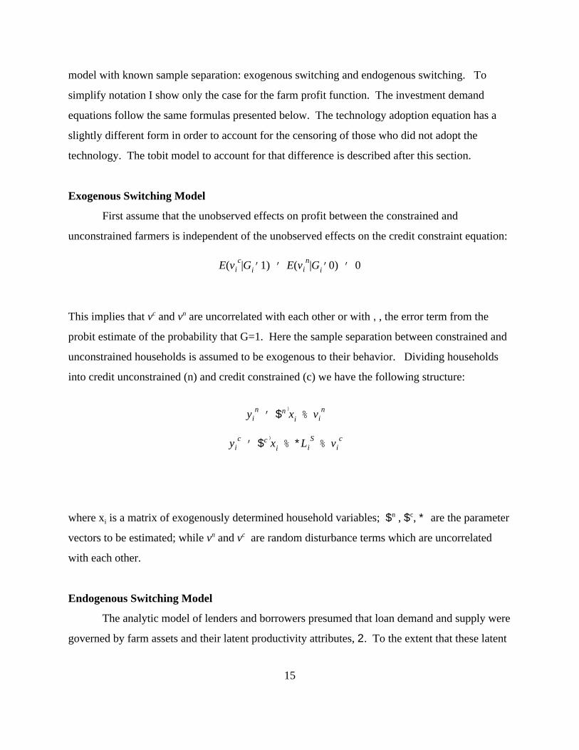
model with known sample separation: exogenous switching and endogenous switching. To

simplify notation I show only the case for the farm profit function. The investment demand

equations follow the same formulas presented below. The technology adoption equation has a

slightly different form in order to account for the censoring of those who did not adopt the

technology. The tobit model to account for that difference is described after this section.

Exogenous Switching Model

First assume that the unobserved effects on profit between the constrained and

unconstrained farmers is independent of the unobserved effects on the credit constraint equation:

This implies that vc and vn are uncorrelated with each other or with ,, the error term from the

probit estimate of the probability that G=1. Here the sample separation between constrained and

unconstrained households is assumed to be exogenous to their behavior. Dividing households

into credit unconstrained (n) and credit constrained (c) we have the following structure:

where xi is a matrix of exogenously determined household variables; $n , $c, * are the parameter

vectors to be estimated; while vn and vc are random disturbance terms which are uncorrelated

with each other.

Endogenous Switching Model

The analytic model of lenders and borrowers presumed that loan demand and supply were

governed by farm assets and their latent productivity attributes, 2. To the extent that these latent

16

y ni ' $n )

xi % v ni iff ()Zi % ,i # 0

y ci ' $c )

xi % *L Si % v c

i iff ()Zi % ,i > 0

productivity attributes are unobservable to the econometrician, they will be among the elements

of the disturbance term v. For example, one would expect that greater farmer skills would

decrease the probability of being credit constrained as well as the realized farm profits. If we

cannot control for farmer skill with observable characteristic, e.g. education, or farming

experience, our distribution term will be correlated with , from the credit constraint equation. In

this case the exogenous sample separation estimation will confound the output effects of farmer

skills with their credit access enhancement effects. The resultant estimated coefficients will be

inconsistent.

Relaxing the constrained version above I let the sample separation be endogenous to the

estimation of the dependent variable. That is I let the fact that a household might be credit

constrained be potentially correlated with the investments, inputs, or profits of that household.

Following Maddala (1983) for the endogenous switching model I assume two regimes with an

endogenous switching equation. For any observation i the relevant structure is:

where the switching equation is the standard probit estimation of whether a household is credit

constrained from the previous section. As researchers we observe only one value of Y dependent

upon which regime that particular individual is in: constrained or unconstrained. The parameters

of the probit equation can only be estimated up to a proportionality constant, so we assume that

the variance of the random disturbance terms will be one: Var( ,i ) = 1. We further assume that

the random disturbance terms vn ,vc, ,i have a trivariate normal distribution, with mean vector

zero, and the following covariance matrix:

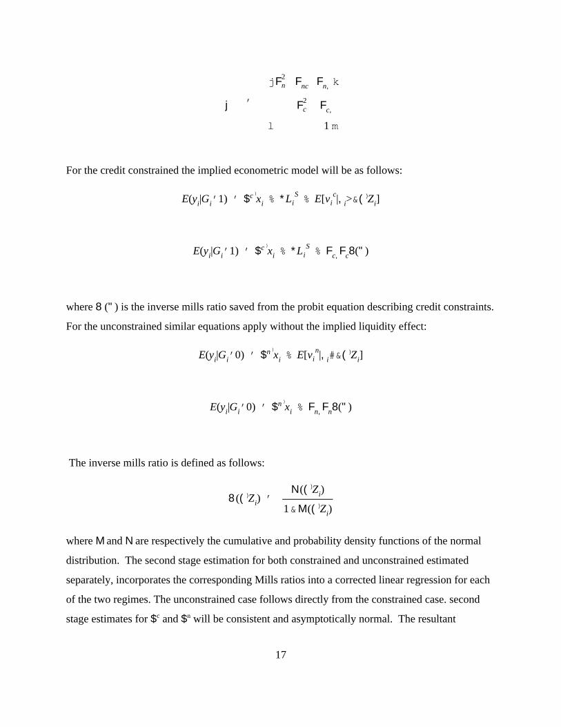
17

j '

j F2n Fnc Fn, k

F2c Fc,

l 1 m

E(yi|Gi'1) ' $c )

xi % *L Si % E[v c

i |,i>&()Zi]

E(yi|Gi'1) ' $c )

xi % *L Si % Fc,Fc8(")

E(yi|Gi'0) ' $n )

xi % E[v ni |,i#&(

)Zi]

E(yi|Gi'0) ' $n )

xi % Fn,Fn8(")

8 (()Zi) 'N (()Zi)

1&M (()Zi)

For the credit constrained the implied econometric model will be as follows:

where 8 (") is the inverse mills ratio saved from the probit equation describing credit constraints.

For the unconstrained similar equations apply without the implied liquidity effect:

The inverse mills ratio is defined as follows:

where M and N are respectively the cumulative and probability density functions of the normal

distribution. The second stage estimation for both constrained and unconstrained estimated

separately, incorporates the corresponding Mills ratios into a corrected linear regression for each

of the two regimes. The unconstrained case follows directly from the constrained case. second

stage estimates for $c and $n will be consistent and asymptotically normal. The resultant

10It is technically possible to estimate this tobit model under endogenous selection. Thesmall number of data points in this sample, however, made these techniques infeasible.

18

A'$)X %, if $)X %, $ 0

A'0 if $)X % , < 0.

ln L ' jAi>0

&1/2[ln(2B) % lnF2 %(Ai&#

)X)2

F2] % j

Ai'0ln[1&Mi(

#)XF

)]

variance-covariance matrix, however, needs correction for heteroskedasticity which is done using

a procedure outlined in the appendix to this paper.

A Tobit Model of Technology Adoption

The technology adoption model follows from the exogenous selection model with the

exception of a correction for sample censoring. I estimate the adoption equation only in the case

of exogenous selection.10

For a given individual, define a dependent variable A as a variable for the amount of the

technology individuals adopt. It can take on the values of zero or a positive value as follows:

where X is a matrix of farm and farmers characteristics, $ is a parameter to be estimated and , is

random disturbance term. One can translate this into a standard tobit model in which the

dependent variable, the amount of land devoted to drip irrigation, is censored at zero for those

who do not adopt the technology. Similar to the binary choice model, one can parameterize

technology preferences in the same fashion as with the binary model, $’X. We assume that the

error term, ,t, is distributed normally with mean zero and variance F2 . Using maximum

likelihood estimation, the log-likelihood function for the standard tobit model is:

where Mi is the cdf of the standard normal distribution function. Here the first part of the

likelihood function is essentially the classical regression model for the non-zero observations,

while the second half represents the probabilities for the censored observations. The maximum

19

likelihood estimator is consistent and asymptotically efficient (Green, 1993).

Estimations of the Effect of Credit Rationing

Having demonstrated the econometric technique, I now turn to the estimation of the

models to test the hypotheses of the effects of credit rationing on profits and investments. In

order test the effects of credit constraints I use the procedure outlined above to estimate a profit

function and an investment demand function. I start with the profit function.

The Table 3 presents the independent and dependent variables used in the estimations.

Those farmers unconstrained in the credit market on average have larger farms, higher

expenditure levels, more agricultural equipment, but lower debt levels and lower overall

profitability. This is a surprising result since one would expect that constrained farmers would

be less profitable and borrow less money. One also sees that the credit constrained have higher

levels of agricultural equipment than the unconstrained, as one might expect from the credit

rationing estimation. In general the variable means do not suggest that credit constraints matter

to profits or even the amount of credit. One should remember, however, that these are

unconditional means and that the estimations will provide a better view of whether credit

rationing matters.

Profit Equation

In estimating farm profits I use net revenue functions, often called pseudo-profit functions

(Carter, 1989) in order to account for possible imperfections in capital, land, and labor markets.

Net revenues differ from economic profits in that they do not account for depreciation costs and

payments to fixed factors, which in this case includes land, family labor, and management. In an

area of imperfectly operating markets farmers will not be able to rent their fixed factors out at a

“market” price. The going market price for a fixed factor might well overstate the real

opportunity costs of using that factor in production. Therefore, valuing profits using market

prices for capital inputs would bias our results. The sample used here has relatively similar

11Most of the differences in input and output prices were based on geographic differences,with 2 towns, Korba and Tazerka, having consistently higher labor costs and marginally lowerinput prices. These differences are picked up in regional dummy variables.

12Loan value as a proxy should under-estimte the true liquidity of a household. An idealmeasure would also include household savings and farm rolling capital funds from the beginningof the season. Farmers were unwilling to estimate this value in the survey.

13At this point the reader may object that wealth proxies liquidity and should only appearin the constrained equation. I include household expenditure, a measure of permanent income, inthe unconstrained equation as a proxy for farmer risk behavior. In a developing country withoutadequate risk markets, profits may be a function of farmer risk tolerance. If farmers exhibitdecreasing absolute risk aversion then risk tolerance will be increasing in income. Thecoefficient on wealth should otherwise be zero or negative.

20

farmers producing similar outputs and facing similar market prices for inputs and outputs.11

Therefore deviations of profits will be due to differences in farmer endowments and access to

markets, particularly the market for capital. Due to the imperfection of markets, farmers will

make profit decisions based on the shadow values of their fixed assets, making quantity a

reasonable proxy variable for the true price of those inputs.

As described above, the appropriate dependent variable describes net revenues of the

farm, while the independent variables will describe farm and farmer characteristics which

influence profits. The regressors for the constrained and the unconstrained are identical to each

other except for a liquidity variable, total loan value, in the equation for the credit constrained.12

Regressors common to the two equations represent farm fixed assets: owned land and capital

equipment; farmer characteristics: education and wealth13; whether a farmer has title to the land

he owns. Since there was relatively little variation in prices among farms, I have dropped price

variables from the equations. The regional dummy variables do, however, pick up some of the

regional variation in prices. The dependent variable, pseudo-profits, is hypothesized to be

increasing in farm fixed assets, farmer education, farmer wealth, and whether the farm has land

title. The credit constrained are expected to have increasing profits in the liquidity variable.

Table 5 shows estimated coefficients for a profit function estimated first assuming

exogenous sample separation and then with endogenous sample separation. Standard errors have

been corrected for heteroskedasticity. The first two columns show the exogenous sample

14The lower end of the 95% confidence bound on the credit constrained coefficient is784.5 while the upper end of the 95% confidence bound for the unconstrained is 213.3.

21

separation model, while the latter two, the endogenous sample separation model. The models

produce fairly high levels of fit, R2 equal to 0.51 and 0.74, for cross-section data with small data

sets. A reasonable number of the coefficients are significant at common levels and have the

expected signs. As predicted a number of the coefficients are different between the credit

constrained and unconstrained equations. This difference, however, is only statistically

significant in the case of the owned land variable.

The estimate of correlation between the error term in our switching equation and the

profit equation is as expected negative. A farmer constrained even though our model predicts he

should not be, will have lower profits than we would otherwise predict. The endogenous

separation model’s estimate of 8, the inverse mills ratio, does not turn out significantly different

from zero suggesting that this formulation has not perfectly described all the variance in

regression switching. The endogenous separation formulation changes the magnitude of a

number of the coefficients in both equations, though it does not change any of their signs. The

large but insignificant values of the endogeneity effect do not support our proposition of

endogenous sample separation. Though the significant difference in the magnitude of some

coefficients suggests that perhaps I have not fully captured all of the endogenous effects.

The results of our estimates for a pseudo-profit function confirm the profit-liquidity

hypothesis. The estimated coefficient on total debts owed is significantly large in magnitude, and

in the case of the endogenous sample separation statistically significant. As might be expected

under imperfectly operating land markets, the amount of owned land is a significant determinant

of overall profits. The significantly larger coefficient on land for the credit constrained suggests

that credit constrained farmers have a higher shadow price for land. These differences are

statistically significant at a 5% level.14 The increased profit (shadow value) a constrained farmer

would receive from renting another hectare of land is greater than the average land rental cost,

while that for the unconstrained is less than rental costs. This implies that liquidity may

constrain the ability to rent or buy land, leading to the divergence of shadow prices. The

estimated shadow price ($2,731 for the constrained and $422 for the unconstrained) for another

22

hectare of owned land brackets the rental values commonly seen in Cap Bon which ranged from

$500 to $3,000.

Of note is the poor performance of agricultural equipment in increasing farm profits once

one takes into account the effects of agricultural equipment on credit access. Neither the

constrained nor the unconstrained gain any profit gain from having better access to family labor.

Having title to land has a positive effect on overall profits for both the constrained and the

unconstrained. The effect appears stronger for the credit constrained, although the two estimates

for the constrained and unconstrained are not different from each other at any reasonable

significance level. Household expenditure level as a proxy for overall household permanent

income also has a positive effect on profits. Again the effect appears stronger for the credit

constrained as one might expect if liquidity effects were present. The differences between the

coefficients between constrained and unconstrained, however, are not statistically significant.

The estimations of the profit function have a number of immediate implications both for

the credit market and for other markets. (1) Better access to the credit market will improve the

profitability of a great number of farmers, though not necessarily the poorest. From the variable

averages it is clear that the constrained are not necessarily those with the lowest profit or who are

the poorest. It seems that the credit constrained might be the high quality producers who can

make the best use of their capital. (2) If credit access were improved, one of the most significant

effects would be in the land market. In fact many of those who claimed they would borrow when

offered a loan would do so to buy or rent land. This increased demand would potentially activate

the land market in the area. The corollary to this is that relaxing credit constraints may lead

toward larger farm sizes rather than productivity increases: increased profitability on a per-

hectare basis. The profit function estimation does not show higher shadow values for family

labor for the constrained nor does it show them for agricultural material. This suggests that

credit constraints may not affect labor or investments.

Investment Demand

In order to test the effects of credit constraints on farm investments the dependent

variable is defined as purchases of capital equipment, new technologies (drip irrigation), and

23

purchased manure. Capital equipment includes investments in tractors and machinery, irrigation

pumps, and green houses. The new technology is drip irrigation, a resource reducing and

production increasing technology. Finally I use manure purchases as a measure of long-term

investments in the land quality of a farm.

We expect that the capital constrained will invest as a function of the capital available to

them rather than their on farm needs. The unconstrained will invest as a function of their farm

needs and their own education level. As would be typical of investment demand functions,

investment should be: increasing and concave in farmer age, increasing in education, decreasing

in fixed assets (capital equipment and family size). Both the constrained and unconstrained are

expected to invest more on land for which they have title.

The estimates of an investment demand function, which I show in table 6, are not very

accurately estimated. The equations fit at a fairly low level (R2 = 0.38 and 0.63). This

formulation does not show direct evidence of a liquidity effect after controlling for the

probability of being credit constrained. In this case, however, the endogenous separation model

does show some merit, with our estimate of the coefficient on the inverse mills ratio significantly

different from zero at a 10% level. These estimated coefficients in general imply that the amount

of money borrowed does not explain investment levels for constrained farmers. However,

household expenditure provides a strong explanation of investments. The estimation of

investment demand for the credit constrained under endogenous credit constraints demonstrates

many of the classic tendencies of investment demand functions. It is increasing and concave in

farm manager age, decreasing in family size, and increasing in income. The puzzling result that

title land leads to less investment disappears when one takes into account the effects of land title

on credit access.

While I do not find a strong liquidity effect in the investment equations, there is a

significant difference in the investment behavior of the constrained and the unconstrained. In the

cases of education and years of farming the estimated coefficients are different from each other at

a 10% and 5% confidence level respectively. A number of the other coefficients are different

across equations, though not significantly so, including family size and owned farm size. This

suggest a number of different behavioral rules in terms of investment demand of the credit

24

constrained and unconstrained. The unconstrained operate as one would expect with more

educated farmers investing more. They also seem to follow a life cycle behavior in their

investments, with it estimated as concave in age. In other words, investments increase with age,

but decreasingly so as a person gets older. Only our measure of household permanent income,

expenditure, is significantly the same sign in both equations. The measure of tenure security,

title, has the same insignificantly negative sign across equations.

Technology Adoption

Having investigated the overall investment decisions of farmers I now disaggregate a part

of that decision to focus on investments in new technologies. The new technology in question

here is a water conserving drip irrigation technology. Some 25% of the total sample adopted drip

irrigation technology. As shown in Foltz (1997) drip irrigation can be highly profitable for these

farmers and reduce their water usage. The dependent variable used in this model is the number

of hectares equipped with drip irrigation technology. This variable equals zero for the non-

adopters (75%) while ranging between zero and two hectares for the adopters.

The independent variables used to describe the adoption decision are similar to those in

the investment equation with a few exceptions. Added to the equation are variables to describe

farmer water usage and farmer knowledge of the technology. As often noted in the literature on

new technologies (e.g. Saha et al. 1994, Shah et al. 1994) information about the new technology

is vital to its adoption. I use as a proxy the number of years a farmer has known about drip

irrigation. The water variable is the farmer’s water cost per hectare the previous year. The

degree of adoption is expected to be increasing in both knowledge and water expenditure. A

number of variables which appear in the other equations are dropped to save on precious degrees

of freedom.

Table 7 presents the results of the tobit estimation of an exogenous selection model for

technology adoption. The estimations are hampered by the small number of data points in each

subsample which leads to a fairly imprecise parameter estimates. They do, however, show some

of the expected patterns, albeit insignificant at commonly used levels. In the constrained

equation, total debt is significant at a 10% level. Its magnitude, though seemingly small, does

15For the credit constrained, the marginal effect of credit accounting for the samplecensoring is [0.91 x 10-5 ]. Using that to calculate an elasticity yields 0.37 of technologyadoption with respect to credit.

25

suggest that large changes, in the thousands of dollars, of credit will influence adoption of the

technology on the order of tenths of a hectare.15 The unconstrained equation shows no

parameters of interest to be significantly different from zero. Overall the results from the

technology adoption equation do find some support for the hypothesis that credit constraints

impinge on farmer technology adoption decisions. While the investment equation alone shows

little effect of credit constraints, the technology part of farmers investment decisions is at least

marginally affected by their liquidity.

V. Discussion

This work set out to test whether Tunisian farmers were constrained in credit markets.

The findings suggest that along a number of different measures of being credit constraints a

significant number of the surveyed farmers did not receive as large loans as they demanded.

Whether a farmer turned out to be credit constrained is a function of both supply and demand

factors. Among the most important supply factors seemed to be land title and household wealth.

Our measures of access to banks, the regional dummy variables, do not suggest that distance

from banks explains farmers being credit constrained. Despite some anecdotal evidence to the

contrary, if there are prohibitive transaction costs in applying for loans, transportation does not

seem to be one of them.

One should note that the most significant factors determining credit status are those that

increase demand. In particular the credit constrained farmers on average had higher profits,

owned less land, and were younger with higher education levels. This suggests that the credit

market is failing the ambitious young farmers rather than the established ones. The

unconstrained seem to fall into the category of those with low incomes, low supply of credit, and

low demand; and the wealthy who can mobilize their own savings. Potentially if it is the young

“middle class” farmer who is constrained in the credit market, Tunisian farming will be less

dynamic. If these are the farmers who might be adopting a new technology, policies to alleviate

26

their credit constraints could greatly increase agricultural potential.

In terms of agricultural policy in Tunisia, the findings here suggest that policies aimed at

alleviating credit constraints will benefit rural areas. Our investigations of credit constraints and

their effects suggests that the presence of credit market constraints does impinge on farm

profitability. Among the more important implications is that the constrained farmers have a

significantly higher shadow price for land than the unconstrained farmers. Therefore, policies to

alleviate credit constraints first and foremost will increase the profitability of credit constrained

farmers. Secondly alleviating credit constraints may activate the rural land markets allowing

peasants to forego potentially exploitative contracting situations. Alleviating credit market

imperfections may also have an impact on technology adoption decisions. Those impacts,

however, remain small and are mitigated by a number of other factors.

Often in the literature it is suggested that agricultural credit is in fact used for

consumption purposes (e.g. Feder et al. 1990). This would suggest that credit rationing affects

primarily consumption smoothing not agricultural productivity, thereby providing a possible

explanation for the poor predictive power of liquidity presented here. The survey results,

however, suggest that the credit constrained were not primarily interested in consumption

smoothing. When asked how they would use a loan, none of the respondents mentioned

household consumption. Only 7 out of the 102 respondents who asked for some sort of loan

wanted to use it for non-agricultural purposes. These 7 were evenly divided between those who

would use the loan for house construction and those who would use it to establish a non-

agricultural business. Neither of these motives for borrowing money suggest that credit was

primarily used in consumption smoothing.

While these estimates provide evidence on the benefits from better credit access

particularly for increasing agricultural profitability, the correct policy to provide loans to farmers

is not as clear. The literature on credit markets suggests that group lending systems may work

well in providing loans to small producers ignored by large banks. These, however, need to be

tailored to the specific institutional and cultural setting of Tunisia in order to be effective. This

research does not provide much guidance as to whether or not such systems would work in this

region of Tunisia. It is left for future research to investigate the optimal type of credit delivery

27

system for rural Tunisia.

Table 1CREDIT SOURCES

ZONE No Debts Debt fromPrivate Sources

BankDebt

Private andBank Debt

Korba 12% 72 4 12

Tazerka 28 64 4 4

Diar Hjaj 28 69 3 0

Lebna 39 47 7 7

Teffaloune 10 80 0 10

Survey 24 64 4 7

Table 2Financial and Credit Status of Households

Financial or Credit Status Percent of SampleHouseholds

1) Have access to $2,000 in their extended family 46 %

2) Have access to $10,000 in their extended family 12

3) Have no access to $2,000 anywhere 4

4) Have no access to $10,000 anywhere 55

5) Have asked for a loan in the last year 26

6) Classified as transaction cost rationed 12

7) Would take a $2,000 loan at 13% interest 62

8) Would take a $10,000 loan at 13% interest 52

9) Defined as credit rationed 45

28

Table 3: Variable Means by Credit Status

Variable Full Sample

CreditConstrained

Unconstrained

Education Level (1-5) 2.28 2.42 2.16

Family Size 6.9 6.9 6.9

Years Farming(Farm Manager)

24 21 26

Agricultural Equip. ($) 4889 5648 4273

Owned Land 2.7 1.2 4.0

Household Expenditureper month

256 209 295

Debts Owed ($) 4941 4064 5654

Land Title [0-1] 0.72 0.69 0.76

Knowledge of tech (yrs) 1.77 1.95 1.62

Water usage ($/hectare) 272 298 250

Profits ($) 11,702 13,624 10,139

Farm Investment:(Technology, Equip.,Manure)

2055 2110 2010

Hectares new technology(drip irrigation)

0.132 0.184 0.10

16Estimation also includes a constant and 2 regional dummy variables. Significance at a5% level denoted by **, the 10% level by *.

29

Table 4Estimated Coefficients of Probit Model:

The Probability of Being Credit Constrained16

Variable Est. Coefficient(t-statistic)

Owned Land (Ha) -0.0283(-0.47)

Agricultural Equipment ($) 0.00002(1.62)

Family Members per hectare ofland

-0.042(-1.05)

Household Expenditure per month ($)

-0.0032 (-3.29)**

Education Level 0.128(1.22)

Land Title [0-1] -0.456(-1.70)*

Log Likelihood -81.43

Percent Correctly Predicted(N=136)

65%

17The dependent variable is defined as total farm profits. Estimation also includes aconstant and 3 regional dummy variables.

30

Table 5:Pseudo-Profit Function Coefficients for Constrained and Unconstrained Households17

Exogenous Separation Endogenous Separation

Variable CreditConstrained

Unconstrained CreditConstrained

Unconstrained

Education -122.5(-0.06)

1724(1.15)

-651(-0.28)

1255(0.75)

Years Experience inFarming

-149(-0.96)

-117(-1.34)

-119(-0.69)

-121(-1.23)

Number of FamilyMembers

-705(-1.25)

-816(-1.86)*

-616(-1.01)

-732(-1.74)*

Agricultural Equipment 0.36(3.99)**

0.51(3.35)**

0.21(0.75)

0.39(1.43)

Owned Land (Ha) 2627.7(2.23)**

464.7(5.29)**

2731(2.75)**

422.3(3.88)**

Expenditure ($/month) 43.2(2.63)**

17.0(1.41)

66.1(1.63)

28.7(1.38)

Total Debts owed ($) 0.788(1.56)

N.A. 0.73(2.40)

N.A.

Title 6697(2.38)**

2409(0.88)

8978(1.62)

4316(1.02)

Lambda -10373(-0.62)

-8056(-0.69)

R-Square[n(cons)=61, n(un)=75]

0.51 0.74 0.52 0.74

18Estimation includes a constant and 3 regional dummy variables.

31

Table 6:Investments18

Exogenous Separation Endogenous Separation

Variable CreditConstrained

Unconstrained CreditConstrained

Unconstrained

Education -704.5(-2.0)

682.4(1.88)*

-838.3(-2.12)**

556.3(1.35)

Years Farming(Farm Manager)

-86.4(-1.26)

150.2(2.03)*

-98.1(-1.45)

179.4(2.46)**

(Years Farming)^2 0.32(0.28)

-2.05(-1.74)*

0.68(0.59)

-2.52(-2.12)**

Family Size -16.9(-0.17)

-252.0(-2.49)**

60.0(0.58)

-243.5(-2.30)**

Agricultural Equip.Owned previously ($)

0.056(2.23)**

0.004(0.08)

0.022(0.57)

-0.05(-0.9)

Owned Farm size 129.4(0.79)

0.015(0.001)

178.9(0.95)

-8.57(-0.35)

Household Expenditure 4.49(1.46)

10.8(6.07)*

9.84(2.18)**

14.8(4.54)**

Debts Owed ($) 0.05(0.99)

0.02(0.39)

Title [0-1] -841.6(-1.43)

-1421(-2.19)**

-204(-0.25)

-672(-0.7)

Lambda -2905(-1.66)

-3322(-1.72)*

R-Square[n(cons)=61, n(un)=75]

0.34 0.60 0.38 0.63

32

Table 7:Adoption of Drip Irrigation: Tobit estimations

Exogenous Separation

Variable CreditConstrained

Unconstrained

Education &0.04(&0.25)

0.14(0.68)

Years Farming(Farm Manager)

&0.016(&1.27)

&0.005(&0.33)

Water Cost ($/hectare) &0.00004(&0.09)

0.0002(0.57)

Years of knowledge ofthe technology

0.02(0.83)

0.11(1.54)

Owned Farm size &0.007(&0.08)

&0.17(&1.51)

HouseholdExpenditure

0.003(0.38)

0.007(1.29)

Debts Owed ($) 0.00003(1.77)*

NA

Log likelihood[n(cons)=61,n(un)=75]

-33.76 -25.61

33

Bibliography

Barham, Bradford; Stephen Boucher, and Michael Carter. 1996. “Credit Constraints, CreditUnions, and Small-Scale Producers in Guatemala.” World Development, 24, pp. 793-806.

Bell, Clive, T.N. Srinivasin, and C. Udry. 1996. "Rationing, Spillover, and Interlinking in CreditMarkets: The Case of Rural Punjab." Typescript. Yale University.

Besley, Timothy. 1995. “Property Rights and Investment Incentives: Theory and Evidence fromGhana.” Journal of Political Economy.103(5). pp.903-937.

Carter, Michael R. 1988. "Equilibrium Credit Rationing of Small Farm Agriculture." Journal ofDevelopment Studies. 28. pp. 83-103.

Carter, Michael R. 1989. “The Impact of Credit on Peasant Productivity and Differentiation inNicaragua.” Journal of Development Economics. Vol. 31. pp. 13-36.

Carter, Michael R., B. Barham, and D. Mesbah. 1996. “Agricultural Export Booms and the RuralPoor in Chile, Guatemala, and Paraguay.” Latin American Research Review 31(1).

Carter, Michael R. and Pedro Olinto. 1996. "Getting Institutions Right for Whom? The WealthDifferentiated Impact of Property Rights Reform on Investments in Rural Paraguay." Typscript. U. of Wisconsin-Madison.

Conning, Jonathan. 1995. "Mixing and Matching Loans: Credit Rationing and Spillover in aRural Loan Market in Chile." Typscript. Yale University.

Eswaran, Mukesh and Ashok Kotwal. 1989. “Credit as Insurance in Agrarian Economies.”Journal of Development Economics. Vol. 31. pp. 37-53.

Feder, Gershon, E. Just, and D. Zilberman. 1984. “Adoption of Agricultural Innovations inDeveloping Countries: A Survey.” Economic Development and Cultural Change. Vol.33, No.2, pp. 255-298.

Feder, Gershon, L. Lau, J. Lin and X. Luo. 1990. "The Relationship between Credit andProductivity in Chinese Agriculture: A Microeconomic Model of Disequilibrium."American Journal of Agricultural Economics. December. pp. 1151-1157.

Foltz, Jeremy. 1997. “The Economics of Water Conserving Technology Adoption in Tunisia: AnEmpirical Estimation of Farmer Technology Choice.” Typescript. U. of Wisconsin.

Foltz, Jeremy. 1998. “Developing Sustainable Agricultural Production: The Diffusion of WaterConserving Irrigation Technology in Tunisia.” Phd Dissertation. U. of Wisconsin.

34

Greene, William. 1993. Econometric Analysis. New York: MacMillan.

Hauge, Soren. 1997. “The Hidden Costs of Rationing in a Chilean Rural Credit Market.”Typescript. University of Wisconsin-Madison.

Jappelli, Tullio. 1990. “Who is Credit Constrained in the US Economy?” Quarterly Journal ofEconomics. 104, pp. 220-234.

Jayarajah, Carl; W. Branson, and B. Sen. 1996. Social Dimensions of Adjustment: World BankExperience, 1980-93. Washington DC: World Bank Press.

Key, Nigel. 1997. “Credit Constraints, Transaction Costs, and Access to Credit in RuralMexico.” Typescript. U. of California-Berkeley.

Kochar, Anjini. 1992. "An Empirical Investigation of Rationing Constraints in Rural CreditMarkets in India." Typscript. Stanford U.

Maddala, G.S. 1983. Limited Dependent and Qualitative Variables in Econometrics. Cambridge: Cambridge University Press.

Milde, Helmuth and John G. Riley. 1988. "Signaling in Credit Markets." Quarterly Journal ofEconomics. February. pp. 101-129.

Mushinski, David. 1995. "Credit Unions and Business Enterprise Access to Credit inGuatemala." Typscript. The College of William and Mary.

Saha, Atanu; H.A. Love; and R. Schwart. 1994. “Adoption of Emerging Technologies underOutput Uncertainty.” American Journal of Agricultural Economics. Vol. 76. No. 3.pp.836-846.

Sethom, Hafedh. 1992. Pouvoir Urbain et Paysanne en Tunisie. Tunis: Ceres Productions.

Shah, Farheed et al. 1994. “Adoption of Irrigation Technology.” in Karla Hoff et al. Eds.Economics of Rural Organization. Oxford: Oxford University Press.

Stiglitz, Joseph and A. Weiss. 1981. “Credit Rationing in Markets with Imperfect Information.”American Economic Review. LXXI, pp.393-410.

World Bank. 1996. Tunisia’s Global Integration and Sustainable Development: StrategicChoices for the 21st Century. Washington DC: World Bank Press.

Zeller, Manfred. 1994. “Determinants of Credit Rationing: A Study of Informal Lenders andFormal Credit Groups in Madagascar.” World Development. no. 22, pp. 1895-1907.

35

[$1

F1,] ' (C )

1C1)&1C )

1Y1

Var[$1

F1,] ' F2

1 (C )

1C1)&1 & F2

1, (C )

1C1)&1C )

1 [D1 & D1Z1(Z)7Z)&1Z )

1D1]C1(C)

1C1)&1

Appendix 1

Correction for Heteroskedasticity in Endogenous Switching Model

As Maddala (1983, pp. 227-8) shows, the estimated variances for the endogenous

switching model will be underestimated if we use a simple heteroskedasticity corrected variances

from OLS. This happens because we would be ignoring the effects of 8(") on the variance of $.

Instead we need to correct for the endogeneity of 8(") in the variance covariance matrix. I

proceed with the explanation for the credit constrained, since the two cases will differ only by the

subscripts used. Let W1 be the vector of 8(") for the credit constrained. Define C1 = (X1 - W1)

and the estimates of the parameters as:

where F1, is the estimated coefficient on the inverse mills ration and Y1 is the dependent variable.

Let N1 be the number of observations in the constrained sample out of a full sample size N and

define the matrix D1 as an N1 x N1 matrix whose ith diagonal element is W1i (W1i + (’Zi) where Zi

is the ith element of the matrix Z . Also define 7 as an NxN matrix whose ith element is equal to

Ni / [ Mi (1- Mi )]. Now define the estimated variance in the following way:

where Z1 is the partition of the matrix Z for those who are credit constrained. For the

unconstrained we can change the subscript and get the result we want.