TS 101 756 - V1.8.1 - Digital Audio Broadcasting (DAB); Registered ...

Coverage Optimizationin Digital AudioBroadcasting Networks
AGNES LIGETI
RADIO COMMUNICATION SYSTEMS LABORATORY


RADIO COMMUNICATION SYSTEMS LABORATORYDEPARTMENT OF SIGNALS, SENSORS AND SYSTEMS
Coverage Optimizationin Digital AudioBroadcasting Networks
AGNES LIGETI
A dissertation submitted tothe Royal Institute of Technologyin partial fulfilment of the degree ofTechnical Licentiate
May 1997
TRITA—S3—RST—9702ISSN 1400—9137ISRN KTH/RST/R-- 97/02--SE

i
Abstract
In OFDM (Orthogonal Frequency Division Multiplexing) based digital audiobroadcasting networks all transmitters can distribute simultaneously the sameinformation using the same frequency block. In such a Single Frequency Net-work (SFN) due to the multipath tolerance of the system within a certain delay,there is a mutual addition of the received signal power from all transmitters.In order to take advantage of this network gain, proper network design isrequired.
In the thesis we focus on the design of SFNs in existing electromagnetic envi-ronment. Our objective is to design a network for distributing a new programover a predefined service area with sufficient signal quality and allowable in-terference level at minimized network hardware cost. The coverage planningtask is formulated as a discrete optimization problem, where transmitter pa-rameters such as power, antenna height and locations are the decisionvariables.
In order to make reliable outage probability estimation by means of sampling(testpoint) techniques, the characteristics of the service area and a number ofsampling techniques are investigated. The proper testpoint distance is shownto be strongly related to the terrain characteristics, propagation model and thetotal outage level. Systematic sampling came out as the best in most of the casestudies. Using stratified sampling based on terrain altitudes and on networkconfigurations did not result in significant improvements.
Different optimization techniques such as heuristics, local search and simulat-ed annealing are investigated and compared. All the algorithms were able tocope with small scale problems. However, in problems with large state spacesimulated annealing outstripped all other algorithms, which confirms that insuch a problem several local minima exist. Minimizing the network hardwarecost when the technical constraints are satisfied gave significant cost reduc-tion. The cost parameters and technical criteria determine the structure of thenetwork. The sensitivity of transmitter positions is also investigated with thehelp of optimization. Refined placement of the transmitters resulted in loweroutage probability, but the improvement decreases with increasing transmitterdensity.

ii

iii
Acknowledgments
First, I would like to thank my advisor Professor Jens Zander, for his guidanceand invaluable comments throughout this work. To both my former andpresent colleagues at the Radio Communication Systems Laboratory, I amgrateful for the friendly and stimulating atmosphere. In particular I am indebt-ed to Göran Malmgren for his valuable and constructive criticism on the thesismanuscript. Special thanks goes to our guest researcher, Seong-Lyun Kim,Mobile Telecommunications Division, Electronics and TelecommunicationsResearch Institute in Korea, for his comments and suggestions regarding opti-mization techniques in Chapter 4 and 5. I am grateful to Lise-Lotte Wahlbergfor her help with all practical issues involved in completing this work. I alsothank Mats Ek, Teracom, for the stimulating discussions.
Finally, I would like to express my gratitude to Zsolt and my parents for theirinexhaustible love, support and encouragement.
The financial support for this work was provided by the National Board forIndustrial and Technical Development (NUTEK), which is hereby acknow-ledged.

iv
v
Contents
Chapter 1 Introduction . . . . . . . . . . . . . . . . . . . . . . . . . . . . . . . . . . 11.1 Radio network coverage design . . . . . . . . . . . . . . . . . . . . 21.2 Service specific characteristics . . . . . . . . . . . . . . . . . . . . 41.3 Related work . . . . . . . . . . . . . . . . . . . . . . . . . . . . . . . . . . 91.4 Scope of the thesis . . . . . . . . . . . . . . . . . . . . . . . . . . . . . 13
Chapter 2 System Models . . . . . . . . . . . . . . . . . . . . . . . . . . . . . . . 172.1 Transmitter network . . . . . . . . . . . . . . . . . . . . . . . . . . . . 172.2 Digital terrain database . . . . . . . . . . . . . . . . . . . . . . . . . 182.3 Propagation model . . . . . . . . . . . . . . . . . . . . . . . . . . . . . 182.4 Interference modeling . . . . . . . . . . . . . . . . . . . . . . . . . . 212.5 Signal-coverage-area prediction . . . . . . . . . . . . . . . . . . 242.6 Design objectives . . . . . . . . . . . . . . . . . . . . . . . . . . . . . . 27
Chapter 3 Outage Probability Estimation . . . . . . . . . . . . . . . . . . 293.1 Outage probability estimation by testpoints . . . . . . . . . 293.2 Service area characteristics . . . . . . . . . . . . . . . . . . . . . . 313.3 Sampling techniques . . . . . . . . . . . . . . . . . . . . . . . . . . . 403.4 Numerical results . . . . . . . . . . . . . . . . . . . . . . . . . . . . . . 46
Chapter 4 Minimal Cost Coverage Planningfor SFN based DAB. . . . . . . . . . . . . . . . . . . . . . . . . . . . 49
4.1 Objective function and state space . . . . . . . . . . . . . . . . 514.2 Algorithms . . . . . . . . . . . . . . . . . . . . . . . . . . . . . . . . . . . 534.3 Performance Results . . . . . . . . . . . . . . . . . . . . . . . . . . . 60
Chapter 5 Practical SFN Planning . . . . . . . . . . . . . . . . . . . . . . . . 695.1 Cost sensitive network planning . . . . . . . . . . . . . . . . . . 695.2 Transmitter location sensitivity . . . . . . . . . . . . . . . . . . . 715.3 Network planning in electromagnetic environment . . . 76

vi
Chapter 6 Conclusions . . . . . . . . . . . . . . . . . . . . . . . . . . . . . . . . . .796.1 Discussion . . . . . . . . . . . . . . . . . . . . . . . . . . . . . . . . . . . .796.2 Future work . . . . . . . . . . . . . . . . . . . . . . . . . . . . . . . . . . .82
References . . . . . . . . . . . . . . . . . . . . . . . . . . . . . . . . . . . . . . . . . . . . .83
Appendix A:Simulated Annealing . . . . . . . . . . . . . . . . . . . . . . . . .89

1
Chapter 1
Introduction
Since the beginning of the twentieth century, audio broadcasting has been go-ing through enormous changes. Due to several driving forces such as thedevelopments of enabling technologies, the increasing quality requirementsand the demands for new services, existing systems have been modernized andnew types of audio broadcasting have been introduced. In the beginning, ma-jority of public radio services were based on HF AM broadcasting, which wasfollowed by VHF FM broadcasting from the sixties. VHF FM broadcastingspread out very quickly due to its reliable and high quality service for fixedreception. Today, the emerging Digital Audio Broadcasting (DAB) can al-ready offer CD quality services both for fixed and for mobile receivers.
Besides the continuous improvement in sound quality for normal programtransmission, there is another trend in the evolution of radio networks. In thebeginning and up to the eighties, radio networks were dedicated (single-pur-pose) networks. In the past few years, other services have been introduced(piggy-backed on existing radio programs) such as paging services, program-associated data services, location-dependent information distribution. In thefuture digital broadcasting will play an important role in interactive multime-dia (including audio, video and data) and internet services, providing thedownlink connection. The reverse communication will probably be imple-mented via other means of communication, such as mobile telephony.
A joint project “Eureka-147” [51] has been launched by the EBU (EuropeanBroadcasting Union) with participations of governmental authorities, scientif-ic institutes and industrial companies in January of 1988 for developing a newdigital audio broadcasting system. In order to investigate the network planningapproaches for terrestrial DAB service, the EBU established a working groupknown as R1/DIG (after a re-organization B/TAP). In the frame of group ac-tivities some simple design rules for DAB planning [48] were established by

2 Introduction
determining (1) the minimum wanted fieldstrength [56] (assuming Rayleighand Gaussian channel, 1.5 MHz DAB signal and 1.5 m receiver height), (2)the required protection ratios and re-use distances between DAB-DAB net-works and between DAB and other services that coexist in the same frequencyband, (3) the type of transmitter and receiver antennas and (4) other practicalnetwork aspects such as utilization of already existing transmitters.
As a major results, the T-DAB Planning Meeting in Wiesbaden [49] providedan allotment plan, which allocates frequency blocks to geographical areas andcountries. Two T-DAB coverages for each country were allowed providingcoverage by one national service area and a joint coverage of the whole coun-try by several non-overlapping regional service areas.1 Most countries havetheir first priority for national or large regional coverage in Band III and theirsecond priority for regional or local coverage in the 1.5 -GHz band. The nordiccountries have their second priority allotments also in Band III.
The DAB service must actually be realized by a new set of transmitters. In thisthesis we focus on cost minimized coverage planning for SFN based DAB net-works over predefined service areas. The coverage design is formulated as anoptimization problem, and we are looking for efficient optimization tech-niques for SFN planning. In the thesis some algorithms are suggested anddifferent SFN specific network characteristics are analyzed.
1.1 Radio network coverage design
An important part of planning any radio communication network is coverageplanning: to ensure that a sufficient signal quality required by the new servicewill be available all over the area where the service is to be offered. Networkcoverage planning involves determining the proper number of transmitters,accurate transmitter locations, radiated power levels, antenna heights, antennapatterns, polarization, frequencies and service dependent parameters — all inorder to satisfy the required service coverage.
During a planning process for a new service there are three types of interfer-ences encountered in the network, which have to be kept at a satisfactory low
1. The allotment gives a country the right to use a frequency block to provide T-DAB service con-taining up to 6 programs within the predefined service area.

1.1 Radio network coverage design 3
level: (1) Internal interference: interference among the transmitters of thenetwork that is subject of the planning. (2) External interference: comingfrom other networks operating in the same frequency range. (3) Generated in-terference: the interference caused by the network to other networks. Thissituation is illustrated in Figure 1-1.
In the early days of radio communication coverage planning was based onsimple rules of thumb such as “the higher power radiated the better” (for min-imizing the number of transmitter sites and thus reducing the cost of theinfrastructure), and that time whole national radio broadcasting networks werebuilt of a very few number of transmitters, operating with extremely high ra-diated power. As the number of independent radio networks offering differentservices — from military systems to public mobile telephony — heavily in-creased, it was recognized that the “brute force” approach of the old daysleaded to pitfalls: the increased interference background level forced new net-works to use even higher power. Such a “power racing” resulted in the quicksaturation of the available radio spectrum, leading to an unnecessary naturalenvironment degradation and capital investment losses. Instead of being lim-ited by the noise, the coverage of the networks become limited by theinterference, and it become necessary to apply sophisticated network planningmethods together with international coordination.
Figure 1-1 Coverage design of a radio network. During planning of a newnetwork coordination with existing networks in the same frequency bandis required. The allowable levels of the three types of interference arestrictly regulated.
1 2
32
2
3
3
11

4 Introduction
Today, radio spectrum is treated as a finite natural resource shared by all coun-tries. Since radio waves do not stop at political borders, the share of thespectrum is subject of international negotiations: the whole — today usable —spectrum is carefully divided into smaller and larger frequency bands, andeach band is allocated to a certain service type usable by one or more coun-tries. Besides of spectrum partitioning, the allowed interference betweendifferent coexisting networks is also regulated, both at national and interna-tional levels.
Despite the fact that the radio spectrum has become saturated, there is still agrowing demand for new radio services. There are two complementing direc-tions to relieve the problem: (1) extending the resource with conquering higherand higher frequency ranges and/or (2) increasing the utilization of the exist-ing resources with better frequency economy. The latter means lowinterference and high frequency reuse. Such economical goals must be keptin mind when designing the coverage for new services. Modern — computersupported — coverage planning methods ensure that the required coveragecan be achieved with using the possible minimal radiated power, hence mini-mizing spectrum pollution.
Making use of the powerful new generation workstations, advanced coverageplanning methods were developed. The advanced methods use digital terrainmodels and database for computerized wave-propagation- and interferencecalculations. In larger networks even advanced optimization methods are ap-plied in order to find the most suitable solution.
1.2 Service specific characteristics
In mobile radio the communication is bidirectional, with dedicated point-to-point “channels”. Therefore the number of served customers is limited by thechannel capacity per transmitter and the density of transmitters. Whereas, dueto the uni-directional point-to-multipoint feature of broadcasting networks, thenumber of receivers is inherently unlimited over the area service is offered.
Concerning traditional FM broadcasting, there are two inherent features of theFM technique that create the main constraints for network planning: (1) It issensitive to multipath propagation which prohibits from the reuse of the same
1.2 Service specific characteristics 5
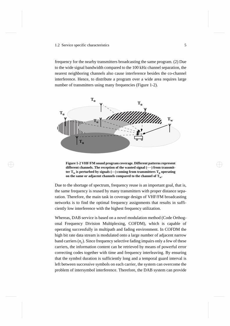
frequency for the nearby transmitters broadcasting the same program. (2) Dueto the wide signal bandwidth compared to the 100 kHz channel separation, thenearest neighboring channels also cause interference besides the co-channelinterference. Hence, to distribute a program over a wide area requires largenumber of transmitters using many frequencies (Figure 1-2).
Due to the shortage of spectrum, frequency reuse is an important goal, that is,the same frequency is reused by many transmitters with proper distance sepa-ration. Therefore, the main task in coverage design of VHF/FM broadcastingnetworks is to find the optimal frequency assignments that results in suffi-ciently low interference with the highest frequency utilization.
Whereas, DAB service is based on a novel modulation method (Code Orthog-onal Frequency Division Multiplexing, COFDM), which is capable ofoperating successfully in multipath and fading environment. In COFDM thehigh bit rate data stream is modulated onto a large number of adjacent narrowband carriers (nc). Since frequency selective fading impairs only a few of thesecarriers, the information content can be retrieved by means of powerful errorcorrecting codes together with time and frequency interleaving. By ensuringthat the symbol duration is sufficiently long and a temporal guard interval isleft between successive symbols on each carrier, the system can overcome theproblem of intersymbol interference. Therefore, the DAB system can provide
Figure 1-2 VHF/FM sound program coverage. Different patterns representdifferent channels. The reception of the wanted signal (—) from transmit-ter Tw is perturbed by signals (---) coming from transmitters Tu operatingon the same or adjacent channels compared to the channel of Tw.
Tw
TuTu
Tu
Tu
Tu
6 Introduction
CD quality radio service to also mobile and portable receivers.
The capability of DAB to overcome multipath interference allows distributinga program over all transmitters in a radio network using the same frequencyblock. A large diversity gain (or network gain) is obtained yielding better cov-erage and frequency economy than in analog broadcasting networks. Thus,one program distribution over a whole country requires only one frequencyblock and one OFDM frequency block can distribute six programs on the 1.5MHz bandwidth.
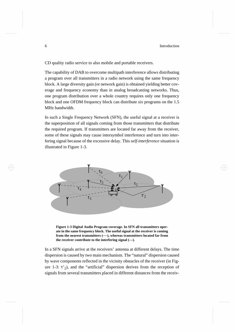
In such a Single Frequency Network (SFN), the useful signal at a receiver isthe superposition of all signals coming from those transmitters that distributethe required program. If transmitters are located far away from the receiver,some of these signals may cause intersymbol interference and turn into inter-fering signal because of the excessive delay. This self-interference situation isillustrated in Figure 1-3.
In a SFN signals arrive at the receivers’ antenna at different delays. The timedispersion is caused by two main mechanism. The “natural” dispersion causedby wave components reflected in the vicinity obstacles of the receiver (in Fig-ure 1-3: τ’2), and the “artificial” dispersion derives from the reception ofsignals from several transmitters placed in different distances from the receiv-
Figure 1-3 Digital Audio Program coverage. In SFN all transmitters oper-ate in the same frequency block. The useful signal at the receiver is comingfrom the nearest transmitters (—), whereas transmitters located far fromthe receiver contribute to the interfering signal (---).
τ1
τ2
τ3τ'2
τ5
τ6
τ4

1.2 Service specific characteristics 7
er. Since the symbol duration is very long compared to the “natural”dispersion, the effect of reflection in the vicinity of the receiver can be neglect-ed. Thus, the intersymbol interference is caused mainly by the “artificial”delay spread. In OFDM systems the extreme delay spread is controlled by us-ing a longer transmitted signal than the actual interval observed by thereceiver. The signal with time interval Ts consist of a useful symbol part withtime interval Tu and a guard interval Tg, see Figure 1-4.
If the delay spread of the signal is smaller than the guard interval, no intersym-bol interference occurs and the signal contribute totally to the wanted signal.Signals arriving later than Ts are treated as interfering signals. Those signalsarriving in between contribute partially both to the wanted and to the interfer-ing signal.
DAB systems proposed by EBU and ETSI has three modes of operation, usingdifferent symbol intervals (Ts, Tu, Tg). The choice of the transmission modedepends on the system operation conditions:
• Transmission mode I is supposed to be used for terrestrial nationalSFNs and local-area broadcasting, in bands I, II and III with a maximumdistance of approx. 100 km between adjacent transmitters.
• Transmission mode II is intended for terrestrial local broadcasting inbands I, II, III, IV and V and in the 1452-1492 MHz frequency range(L-band). It can also be used for satellite-only and hybrid satellite-ter-restrial broadcasting in the L-band.
Figure 1-4 a) The transmitted symbol Ts. The symbol consists of the basicsymbol Tu and the guard interval Tg. b) Multipath delayed signals in com-parison with the window Tu used for detection in the receiver.
Tu Tg
τo
Transmitted signal Received signals
Receiver window
τo+Tu
b,a,
8 Introduction
• The intended application of transmission mode III is the introductionof satellite and hybrid satellite-terrestrial broadcasting below 3GHz.Mode III is also preferred for cable distribution because it can be usedat any frequency available on cable.
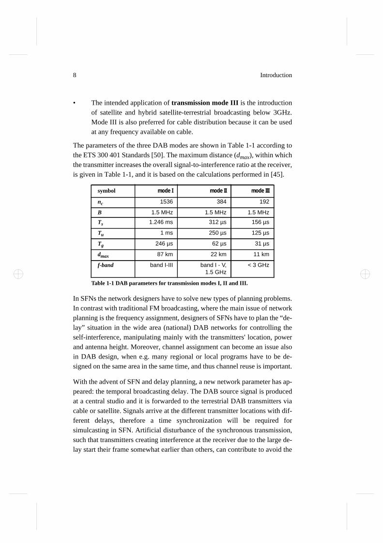
The parameters of the three DAB modes are shown in Table 1-1 according tothe ETS 300 401 Standards [50]. The maximum distance (dmax), within whichthe transmitter increases the overall signal-to-interference ratio at the receiver,is given in Table 1-1, and it is based on the calculations performed in [45].
In SFNs the network designers have to solve new types of planning problems.In contrast with traditional FM broadcasting, where the main issue of networkplanning is the frequency assignment, designers of SFNs have to plan the “de-lay” situation in the wide area (national) DAB networks for controlling theself-interference, manipulating mainly with the transmitters' location, powerand antenna height. Moreover, channel assignment can become an issue alsoin DAB design, when e.g. many regional or local programs have to be de-signed on the same area in the same time, and thus channel reuse is important.
With the advent of SFN and delay planning, a new network parameter has ap-peared: the temporal broadcasting delay. The DAB source signal is producedat a central studio and it is forwarded to the terrestrial DAB transmitters viacable or satellite. Signals arrive at the different transmitter locations with dif-ferent delays, therefore a time synchronization will be required forsimulcasting in SFN. Artificial disturbance of the synchronous transmission,such that transmitters creating interference at the receiver due to the large de-lay start their frame somewhat earlier than others, can contribute to avoid the
symbol mode I mode II mode III
nc 1536 384 192
B 1.5 MHz 1.5 MHz 1.5 MHz
Ts 1.246 ms 312 µs 156 µs
Tu 1 ms 250 µs 125 µs
Tg 246 µs 62 µs 31 µs
dmax 87 km 22 km 11 km
f-band band I-III band I - V,1.5 GHz
< 3 GHz
Table 1-1 DAB parameters for transmission modes I, II and III.

1.3 Related work 9
problem of self-interference. Probably, using “precasting” for transmitters lo-cating near to the edge of the service area can improve the overall receptionquality in the service area.
As all frequency bands considered for DAB are already occupied by other ser-vices, an extensive coordination will be necessary. In the VHF range threeimportant type of interference have to be considered: DAB interferences withDAB, television and military aeronautical services. In general, the DAB signalis more robust against interference from other services than vice-versa. Hence,the interference effect into the DAB channel is less critical than the causedinterference.
1.3 Related work
The coverage design of audio broadcasting networks involves different areasas wave-propagation using digital terrain database, interference modeling,continuous and discrete optimization techniques and service characteristics.
The selection of the digital terrain database parameters such as grid size, inter-polation methods has a strong influence on the prediction error. In [2] theseparameters are analyzed. Using spectral estimation technique a grid size of
m2 is suitable for representing the mountain areas, whereas for flatterrain a grid size of m2 seems to be enough in order to keep theheight standard deviation error below 5 m. Eight different interpolation meth-ods are compared in the paper. The linear interpolation using four pointsresulted in as good approximation error as more sophisticated methods duringmuch shorter time. The estimation error due to the interpolation error in thecoverage prediction are found 5-6 dB secondary compared the errors includedin the propagation models themselves.
According to the national and regional DAB frequency range, channel 12-13(~230 MHz), our literature study on wave propagation models is confined tothe VHF range. A great number of different methods for the local mean field-strength prediction over irregular terrain has been developed in the last years[3]-[17]. A comprehensive comparison study of today existing 2D propaga-tion models is given by Grosskopf [11][12], and Perez-Fontan and Hernando-Rabanos [13].
50 50×500 500×

10 Introduction
The propagation models are categorized as area propagation models andpoint-to-point propagation models. In area propagation models the mediantransmission loss calculations are based on generalized characteristics of theareas surrounding the transmitter and receiver. The point-to-point propagationmodels calculate the median transmission loss based on specific characteris-tics of the path between the transmitter and the receiver. The CCIR [3],Okumura and the “Longley and Rice” [4] models belong to the first category,while “Durkin and Edwards”, “Blomquist and Ladell” [8][9], and diffractionmodels from Deygout [6], Epstein-Peterson [10], Bullington [5], Giovaneli [7]are “point-to-point” propagation models.
In many point-to-point models the transmission loss consists of a theoreticalestimate modified by an empirical correction factor due to the terrain irregu-larity and vegetation. The terrain profile is replaced by a series of the mostprominent features represented by ideal knife-edges or rounded obstacles anddiffraction fields from other obstacles can be neglected. The transmission lossdue to the multiple knife edges is estimated by several methods based on theapplication of geometric optics and the single knife-edge diffraction lossmodel.
New approaches have been developed using powerful computers and more ac-curate 3D-databases with high resolution. They model more realistically theTransmitter-Receiver (T-R) profile by replacing the knife-edges by wedgesand convex surfaces to model obstacles in the profile [15]; and the fieldstrength calculation by geometric theory of diffraction is based on point-to-point ray tracing [14][16]. In a very irregular terrain, reflection and scatteringfrom the terrain obstacles vertical to the 2D-profile can yield severe additionalpath loss. Therefore, the 2D model is extended to 3D including bistatic scat-tering from the terrain on the vertical T-R plane using theories from physicaloptics [17].
The exact statistical treatment of the total field constructed by several individ-ual lognormal shadowed signals is very hard to carry out numerically. For thatreason a number of approximation have been developed for determining thepower sums of log-normal stochastic variables. The Power Sum Method, theSimplified Multiplication Method [19], and the Log-Normal Method are com-monly used in broadcasting practice. A comprehensive description of the mostcommon methods is given in [18] and they are compared in [20][21]. An ap-
1.3 Related work 11
proximate technique for the evaluation of the mean and the variance of thepower sums with log-normal components are presented by Schwartz and Yehin [22].
Description of the service area by the representative terrain area elements(called testpoints) is a commonly used method in network design. Differenttypes of selection methods are presented in the literature. In paper [28] for de-signing VHF networks, the testpoints are selected in pairs, i.e. for each pair oftransmitters two critical testpoints are determined. In the wanted coveragearea of each transmitter one testpoint that suffers most from interference of theother transmitter (lowest carrier-to-interference ratio) is selected. Contrary to[28], the method in [29] is based on the generalized concept for description ofthe electromagnetic environment. There, testpoints represent towns, commu-nities, transmitter locations and other highly protected locations. Thus, theyare not associated with a certain transmitting station, instead they represent acertain area of the country.
The coverage optimization problem consists of frequency, power, transmitterantenna-height and transmitter location assignment tasks. The goal of the cov-erage optimization is to minimize the interference in the network, namely torealize an acceptable interference in order to offer a reliable coverage. The fre-quency assignment itself is equivalent to the generalized graph coloringproblem, which is an NP complete problem. Using this equivalence and recentresults concerning the complexity of graph coloring, Hale in [37] classifymany frequency assignment problems (frequency-distance constrained, fre-quency constrained etc.) according to the execution time efficiency ofalgorithms that may be devised for their solution.
Modeling the power, transmitter antenna-height and transmitter location as-signment problems as a discrete valued problem, the coverage optimizationproblem becomes a discrete optimization problem [30][32], that falls in thecategory of NP-complete problems, i.e. in the worst case it is not solvable inpolynomial time. In order to find satisfying solution for coverage optimizationmany approximation or heuristic algorithms were developed, for which thereis usually no guarantee that the solution found by the algorithm is optimal, butfor which polynomial bounds on the computation time can be given [33].
Simulated Annealing [34][35] is an approximative optimization technique.

12 Introduction
The algorithm is based on randomization techniques and also incorporates anumber of aspects related to iterative improvement algorithms. These algo-rithms determine the definition of configurations, an objective function and ageneration mechanism, i.e. a simple prescription to generate a transition froma configuration to another one by a small perturbation (neighborhood). Simu-lated Annealing is a derivative of the Monte-Carlo method proposed byMetropolis, and is based on the analogy between the simulation of the anneal-ing of solids. The convergence behavior of the algorithm and the mathematicalproofs can be found in [36]. The first attempt to use the Monte-Carlo methodfor VHF FM frequency assignment is presented in [37]. Simulated Annealingwas successfully applied in planning of the conventional FM broadcasting[39][40][41], and also in mobile systems [42][43].
Using a new modulation scheme COFDM (Code Orthogonal Frequency Divi-sion Multiplexing) [44][46], DAB is able to overcome the multipathinterference offering reliable service for mobile receivers. The “artificial”multipath situation provided by the single frequency feature can be changed todiversity gain with the coding technique, resulting in improved coverage.DAB has successfully passed the first pilot projects, commercial introductionis planned from 1996. A set of European standards is already available [50],which helps in spreading the new service.
There are several reports on network planning for DAB [52][53][54]. For thefirst implementations existing FM transmitter sites are used. Propagation cal-culations are based on properly adapted CCIR models (receiver antenna heightis 2 m, required coverage is 99 %, etc.). More refined DTM-based models arealso reported. [45] gives a comprehensive study on interference calculationsfor DAB networks. Pilot projects include both national (DAB Mode I) and lo-cal (Mode II) networks. In national networks high frequency utilization andexcellent sound quality have been proved already in the practice, while theanalysis of local networks require further efforts. Re-use distance determina-tion, ideal network topology for local networks (number of transmitters,optimal power, optimal antenna height etc.) are among the open issues. Sev-eral article address these topics [55][59]-[62] establishing different methodsfor finding design parameters.
By using single frequency network with a high number of transmitters for cov-ering the service area, the frequency reuse distance can be reduced
1.4 Scope of the thesis 13
considerably due to the following effects: (1) The closer the individual trans-mitters of the SFN are located the less power and the less high antennas needto be used, which decreases the interference caused by the network for the sur-rounding areas. (2) Use of directional antennas pointed towards the centre ofthe SFN reduces the interference to neighboring SFNs. (3) The high numberof transmitters in the network increases the network gain, that results in a low-er required power level.
A detailed investigation to maximize the size of the service area of a SFN ispresented in [64]. As decision variables, the network parameters such as themaximum ERP, the temporal broadcasting offset and the antenna pattern areapplied and they can be assigned for each transmitter individually during theoptimization process. The number and the location of the transmitters havebeen fixed before the optimization. The optimization is performed in threesteps, creating an optimization phase for each type of the decision variables.As optimization method the “great deluge” global approximative algorithm isimplemented. The service area is described via 3000 testpoints. The resultsshow that it is more efficient to use a large number of low-power transmittersthan only a few with high ERP.
1.4 Scope of the thesis
In the thesis our focus is on the optimization of digital audio broadcasting net-works. In our formulation the goal is to establish a transmitter network in anexisting electromagnetic environment, in order to distribute a new programover a predefined area (called service area) with a sufficient signal qualitymeasured by the outage probability and allowable interference level, with theminimized network hardware cost. The cost is defined by the power, antennaheight and transmitter site cost. We formulate the coverage planning as an op-timization problem, where the antenna parameters such as power, antennaheight and site construct the decision variable of the problem and the objectivefunction is given by the collective cost of the transmitters in the network. Theoutage probability constraints are included in the objective function as a pen-alty, creating an unconstrained discrete optimization problem.
The calculation of the outage probability is based on computerized wave prop-agation models using digital terrain database, interference modeling and

14 Introduction
coverage calculations. Without loss of generality we have chosen two propa-gation models — an area prediction model CCIR [3] and a point-to-pointmodel Blomquist and Ladell [8][9] —, which are commonly used in the radioengineering practice. For calculating the interference and coverage in DABnetworks the ETSI DAB standard [50] and CCETT interference model [45]are used.
The outage probability estimation is based on the measurements or estimationof the service quality in certain terrain area elements (test points) of the targetservice area. For the digital service, calculation of the bit-error rate using theSIR is not in the scope of the thesis. In order to decrease the necessary numberof coverage calculations appropriate sampling techniques are to be found. Weinvestigate the characteristics of the coverage area in the first part of the thesis.The coverage area constructs a correlated population in space. The spatial cor-relation of the outage is strongly related to the terrain characteristics,propagation model and the level of the total outage. Our goal is to determinethe dependency of the local outage based on the terrain and transmitternetwork.
The outage probability estimation in a selected number of terrain elements isa sampling problem. We investigate different sampling processes such as sim-ple random sampling, systematic sampling, stratified simple random samplingbased on the terrain, stratified simple random sampling based on the transmit-ter network structure and sequential sampling.
In the second part of the thesis we take the challenge to discover efficient op-timization algorithms for SFN planning, using different optimizationtechniques such as probabilistic approximative algorithm Simulated Anneal-ing, two types of Local Search techniques and heuristics algorithms. In SFNsthe power, antenna-height and transmitter sites create the state space for theoptimization, together with the total number of transmitters. With the optimi-zation our goal is twofold: on the one hand to develop efficient algorithms forSFN coverage design, on the other hand to discover the inherent features ofdigital audio broadcasting networks.
The main contributions of the thesis are:
• Throughout analysis of the spatial characteristics of the coverage (out-age) in SFNs

1.4 Scope of the thesis 15
• Derivation of optimal sampling strategies for outage probabilityestimation
• Cost based coverage design formulated as a discrete optimizationproblem
• Efficiency comparison of a number of optimization techniques, includ-ing simple heuristics, local search and simulated annealing for theproblem
• Identification of a number of simple design rules via optimizationexperiments

16 Introduction

17
Chapter 2
System Models
This chapter describes the modeling assumptions that is used for coverage de-sign in the thesis, including the following items: transmitters, terrain,propagation, interference, coverage estimation and design objectives.
2.1 Transmitter network
Generally, the factors by which radio communication networks are deter-mined are: operating frequency, radiated power, transmitter location, antennaheight, radiation pattern, polarization, receivers and modulation. In the thesisbroadcasting networks are modeled in the following way: A transmitter in anSFN is characterized by the following set of operational parameters:
• frequency (f)
• transmitted power (p)
• antenna height (h)
• location (s)
• and radiated program (g).
The transmitters are divided into two groups, according to their role in the cov-erage design: (1) New transmitters are subject of the coverage planning, i.e.their parameters (at least some of them) provide the grade of freedom to thecoverage optimization process. Note, that the number of transmitters itself isalso often a free parameter. New transmitters may or may not serve the samebroadcasting program. (2) Existing transmitters form the electromagneticenvironment, in which the new transmitters have to be embedded. Their inter-ference to the new service area and the interference from the new transmittersto their served area have to be considered. Their operational parameters how-ever, cannot be changed. Existing transmitters can be either transmitters of

18 System Models
other services (programs) that operate in the same frequency band as the newservice or can be existing transmitters of the new service that are already inoperation.
Parameters of a transmitter are grouped to the following touple ti which unam-biguously describes transmitter i.
(2-1)
The sets of and de-note the set of new transmitters and existing transmitters, respectively. nN isthe number of new transmitters, while nI is the number of existing transmitters.The number nN and the parameters of transmitters in set N are the subject ofthe coverage design. The set N is called network configuration. During theplanning process, a large number of configurations are evaluated in order toselect one, which optimal fit to our requirements. The set of all possible net-work configurations will be denoted by Ω.
2.2 Digital terrain database
In radio communication system planning tools a large variety of digital terraindatabases are applied. They contain information about the topography, themorphology divided into land usage categories (such as water, forest, open ar-ea, suburban, city etc.) and about the population distribution. Matrixrepresentation ranging from 1000x1000 m2 to 50x50 m2 grid size are used torepresent the relief. Natural or artificial obstacles such as rivers, roads or bor-der of a city, county and country are usually stored in vectorized form.
The terrain database applied in the thesis contains only altitude information inrasterized form, where one raster (also called segment) corresponds to an areaof . For constructing terrain profile between the receiver andthe transmitter linear interpolation is used.
2.3 Propagation model
A great number of different methods for the local mean field-strength predic-tion over irregular terrain have been developed. Because of the complexity of
ti f i pi hi si gi, , , ,⟨ ⟩=
N t1 t2 … ti … tnN, , , , , = I t1 t2 … ti … tnI
, , , , , =
250m 250m×
2.3 Propagation model 19
the 3D and ray-tracing propagation models we will confine ourselves to the2D-methods. In the thesis, CCIR model as an area propagation model is ap-plied, because this model is used in the international broadcastingcoordination. Comparison studies in [11][12][13] have shown that the modelfrom Blomquist & Ladell yields a relatively good accuracy with the smalleststandard deviation and a mean prediction error near to zero, which led us tochoose this model as a point-to-point model in our coverage prediction.
2.3.1 CCIR model
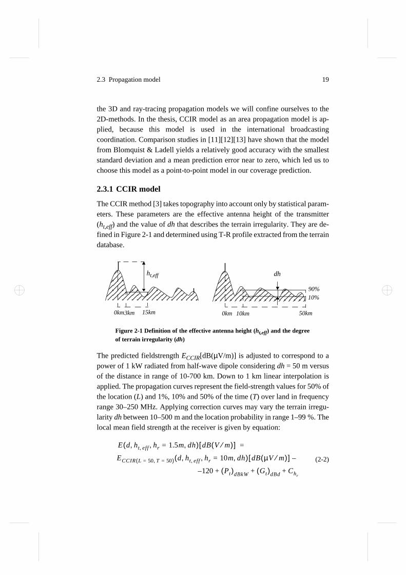
The CCIR method [3] takes topography into account only by statistical param-eters. These parameters are the effective antenna height of the transmitter(ht,eff) and the value of dh that describes the terrain irregularity. They are de-fined in Figure 2-1 and determined using T-R profile extracted from the terraindatabase.
The predicted fieldstrength ECCIR[dB(µV/m)] is adjusted to correspond to apower of 1 kW radiated from half-wave dipole considering dh = 50 m versusof the distance in range of 10-700 km. Down to 1 km linear interpolation isapplied. The propagation curves represent the field-strength values for 50% ofthe location (L) and 1%, 10% and 50% of the time (T) over land in frequencyrange 30–250 MHz. Applying correction curves may vary the terrain irregu-larity dh between 10–500 m and the location probability in range 1–99 %. Thelocal mean field strength at the receiver is given by equation:
(2-2)
Figure 2-1 Definition of the effective antenna height (ht,eff) and the degreeof terrain irregularity (dh)
3km 15km
ht,eff
10km 50km
dh
90%10%
0km0km
E d ht eff, hr 1.5m= dh, , ,( ) dB V m⁄( )[ ] =
ECCIR L 50 T 50=,=( ) d ht eff, hr 10m dh,=, ,( ) dB µV m⁄( )[ ] –
120– Pt( )dBkW Gt( )dBd Chr+ + +
20 System Models
where Pt is the transmitted power and Gt is the antenna gain of the transmitter.CCIR Recommendation 370 curves are related to a receiving antenna heightof 10 m above ground, whereas a terrestrial DAB (T-DAB) service will beplanned primarily for mobile, i.e. with a receiving antenna height of about1.5 m. Measurements performed show that a correction factor ( ) of 10 dBis necessary.
2.3.2 Blomquist and Ladell model
A semi-empirical model by Blomquist and Ladell [8][9] has been developedfor frequency range 30–1000 MHz. The model consists of several basic prop-agation models such as propagation over smooth spherical earth (Ls),diffraction by multiple knife edges according to the “Epstein-Peterson” model(Ld), and empirical loss model for vegetation and urban areas. The model as-sumes digital terrain database to provide the topological and morphologicalinformation. Considering our available database we are dealing with only thealtitude information.
At low frequencies the electrical properties of the obstacles are the most deter-mining factor. The terrain irregularities can be neglected and the basictransmission loss is given by the smooth spherical earth model. With increas-ing frequency the wave behaves as light and its properties can be determinedin terms of optics. The diffraction by hills and mountains becomes the domi-nant propagation mechanism. In the “Blomquist and Ladell” model these twofactors are included in the propagation loss by a bridging function, which isthe square root of the sum of the squares of these two components. The totalpropagation loss (Ltot) in [dB] is given in equation (2-3) includes also the freespace transmission loss (Lfs). Parameters d and λ are the distance between thetransmitter and the receiver, and the wave-length in [m], respectively.
(2-3)
The local mean field strength at the receiver is given by equation (2-4), wherethe quantity Zo is the impedance of free space and equals 377.
(2-4)
In order to evaluate the influence of using structural and effective antennaheights, prediction error has been analyzed for both cases in [13]. The results
Chr
Ltot L fs Ls2
Ld2++= where L fs 20 lg 4πd λ⁄( )⋅=
E( )dB Pt( )dB Gt( )dB 10lg Zo( ) Ltot( )dB 10lgλ2
4π------
––++=
2.4 Interference modeling 21
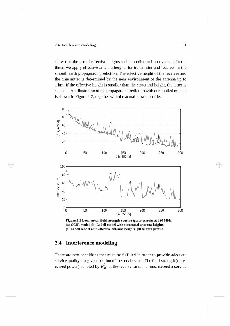
show that the use of effective heights yields prediction improvement. In thethesis we apply effective antenna heights for transmitter and receiver in thesmooth earth propagation prediction. The effective height of the receiver andthe transmitter is determined by the near environment of the antenna up to1 km. If the effective height is smaller than the structural height, the latter isselected. An illustration of the propagation prediction with our applied modelsis shown in Figure 2-2, together with the actual terrain profile.
2.4 Interference modeling
There are two conditions that must be fulfilled in order to provide adequateservice quality at a given location of the service area. The field-strength (or re-ceived power) denoted by at the receiver antenna must exceed a service
Figure 2-2 Local mean field strength over irregular terrain at 230 MHz(a) CCIR model, (b) Ladell model with structural antenna heights,(c) Ladell model with effective antenna heights, (d) terrain profile.
0 50 100 150 200 250 3000
20
40
60
80
100
d in 250[m]
E[d
B(u
V/m
)]
0 50 100 150 200 250 3000
20
40
60
80
100
d in 250[m]
Alti
tud
e in
[m
]
d
b
ca
EW2

22 System Models
specific noise ( ) and interference level ( ). We assume that the qualityof the received signal at a given location (x,y) depends only on the Signal-to-Interference Ratio (SIR), denoted by Γ and defined as
. (2-5)
A general signal environment in SFN comprises nw wanted useful fields Ew,i,i = 1...nw, and nu unwanted interfering fields Eu,i, i = 1...nu, and noise fieldstrength EN. Thus, (2-5) can be rewritten as
. (2-6)
The useful signal at the receiver is the part of the total signal power that fallswithin the receiver window. The unwanted field consists of two parts, the firstpart is the power from the transmitters of the network that due to the signal de-lay overlaps with the following symbol and the second part is the interferingpower from external transmitters transmitting different program on the samefrequency block. The SIR can then be written as a function of the propagationdelay between the receiver and all the transmitters:
. (2-7)
The ratio between the useful and interfering contribution of a given signal isdecided by a weighting function w(τi – τo), according to the delay of the signal(τi – τ0). For the weighting function we apply the quadratic function that wassuggested in [45], shown in Figure 2-3 and described by Table 2-1. The sym-bol τi is the time of arrival of the signal from transmitter i at the receiver. Thetotal useful power depends on the starting point τ0 of the receiver detectionwindow. The time synchronization concerns the precise generation of the FFTwindow and can be considered as both a frame and a symbol synchronization.For frame synchronization the detector will use a special symbol (called “null”
EN2
EU2
Γ x y,( )EW
2x y,( )
EU2
x y,( ) EN2
x y,( )+------------------------------------------------=
Γ x y,( )
Ew i,2
i 1=
nw
∑
Eu i,2
i 1=
nu
∑ EN2+
--------------------------------=
Γ x y,( )Ei
2w τ i τ0–( )⋅
i N∈∑
Ei2 1 w τ i τ0–( )–( )⋅
i N∈∑ Ei
2
i I∈∑ EN
2+ +----------------------------------------------------------------------------------------------=

2.4 Interference modeling 23
symbol) in the frame. For symbol (precise time) synchronization the generalcriterion is to maximize the Signal-to-Interference Ratio. The receiver has tochoose the starting point of the window in such a way that the useful receivedpower from the signals has to be as high as possible besides of minimizing theoverall interfering power. This starting point will be called the time synchro-nization point.
In our model we assume a very simple receiver, where the window starts at thearrival of the first received signal plus the guard interval Tg. The difficulties ofthe synchronization in the presence of pre-echoes and post-echo are discussedin [47].
Figure 2-3 Weighting of the received signal power depending on the delayof the signal to the synchronization time.
Delay w(τ)
Table 2-1 Weighting function
Tg Tg+Tu
w τ( )
τ
Eu,i2 = Ei
2(1 – w (τi – το))
Ew,i2 = Ei
2 w (τi – το)
τ T u–≤ 0
T u– τ 0≤ ≤T u τ+
T u---------------
2
0 τ T g≤ ≤ 1
T g τ T u T g+≤ ≤T u τ T g+–
T u---------------------------
2
τ T u T g+≥ 0
24 System Models
2.5 Signal-coverage-area prediction
The coverage property of a given network configuration is measured by theoutage probability denoted by po, and defined as
(2-8)
within the target service area (denoted by A), where γo is the protection ratio,i.e., the minimum required SIR to provide the required reception quality.
When the pair of RVs (x, y) are uniformly distributed over the service area, theoutage probability is the area outage probability defined by equation (2-9).
(2-9)
In the other hand, if the RVs (x, y) describe the location of the users with dis-tribution function fxy(x, y), po is the population outage probability.
It has been determined from experiment that the field strength obeys certaindistribution laws which specify its behavior in space and time. The locationvariation of a single field strength E can be modeled by a log-normal distribu-tion due to the prediction error [11]. Concentrating on the location variability,this distribution is given by
(2-10)
where the field strength is defined in dB, . According to themeasurements in [58] a standard deviation of location of 6.5 dB is assumed,when CCIR propagation model is applied. This value is more suitable for 1.5MHz wide band DAB signal than the suggested 8.3 dB for FM narrow bandsignal in the CCIR Rep. 945-2 [18]. Due to the better estimation for Ladellmodel [11] the location standard deviation of 4.0 dB is applied.
For most systems the fieldstrength at a given reception location varies alsorandomly with time. These temporal fluctuations are caused by the variationwith time of the refraction, reflection, diffraction, absorption and scattering
po Pr Γ x y,( ) γo< f xy x y,( )⋅ xd ydx( y ) A∈,
∫∫=
po1A--- Pr Γ x y,( ) γo< xd yd
x( y ) A∈,∫∫=
f F η σ,( ) 1
2π σ⋅------------------ F η–( )2–
2σ2-----------------------
exp⋅=
F 10 E2( )10log=
2.5 Signal-coverage-area prediction 25
phenomena in the troposphere and ionosphere or by the movement of the re-ceiver. Time percentage is usually embedded in the wave propagation models,otherwise it may be neglected assuming 100% for the time fraction.
We assume, that the fieldstrength at a given location is characterized by a log-normal distribution. In this case we can determine the probability of coverage(pc) in a small area around the point (x, y) as
. (2-11)
Due to the interference behavior of the system, the total interference field EU2
consists of the sum of several log-normally distributed random variables. Thesame can be said about the wanted signal.
The exact statistical treatment of the total field is very hard to carry out numer-ically. Approximation methods have been developed for determining thepower sums of log-normal stochastic variables. In our study we consider theLog-Normal-Method described in [18], which is often applied in the broad-casting planning practice, and gives quite accurate result according to thecomparison in [20][21] among methods described in [18].
Log-normal method
This method is based on the following assumptions: (1) the field strengths Fi
from all transmitters are independent identically distributed (i.i.d.) normal ran-dom variables with σ standard deviation, (2) the signals are replaced by oneresultant field strength ET which is subject to the log-normal distribution, i.e.,FT has a normal distribution with mean
(2-12)
and standard deviation
(2-13)
with
(2-14)
pc x y,( ) Pr Γ x y,( ) γo> PrEW
2
EU2
EN2+
--------------------- γo>
= =
ηT 0.1152σ2 10lg Ei2
i∑
5lg U( )–+=
σT 6.58 lg U( )⋅=
U
k 1–( ) Ei2
i∑
Eii
∑ 2
------------------------------ 1+= and k σ 4.34⁄( )2[ ]exp= .

26 System Models
The total useful and interfering field strength can be described by log-normaldistribution with parameters ηW, σW and ηU, σU respectively. Different ap-proximate treatments have been investigated in [21] for determining thecoverage probability. In one approach the noise is considered as an interferingfield and it is included in the total field strength as a similar component to theinterfering incoming signals. In this case the SIR Γ(x,y) in dB has normal dis-tribution N( ) with parameters and
, and it is possible to evaluate the expression (2-11),
(2-15)
where is the normal distribution function. We assume that there is nocorrelation between the total useful and interfering signal, i.e. . This as-sumption is not really true in SFN, where due to the contribution of a signal asboth useful and interfering, there is a correlation between the total useful andinterfering field.
For noise limited system the coverage probability can be written as
(2-16)
where the effect of the noise and interference are considered independently.
The service coverage at a given location is achieved if and only if
(2-17)
where pc,min is the system specific probability threshold which for a DAB sys-tem is 0.99. In contrast to analog broadcasting, where pc,min = 0.50, such highthreshold is required due to the rapid degradation of the reception quality incase of insufficient SIR.
Γ x y,( ) σΓ x y,( ), Γ x y,( ) ηW ηU–=σΓ
2 σW2 2ρσWσU– σU
2+=
pc x y,( ) Pr Γ x y,( ) γo> 1
2πσΓ
----------------- Γ Γ–( )2–
2σΓ2
-----------------------
exp⋅γo
∞
∫ dΓ==
1 Φγo Γ–
σΓ------------
– ΦΓ γo–
σΓ--------------
12--- 1 erf
Γ γo–
2σΓ
--------------
+
⋅= = =
Φ •( )ρ 0=
pc x y,( ) Pr EW2
EU2⁄ γo> Pr EW
2EN
2⁄ γo> ⋅= =
ΦηW ηU– γo–
σΓ--------------------------------
ΦηW FN– γo–
σW--------------------------------
⋅=
pc x y,( ) pc min,≥

2.6 Design objectives 27
In the thesis we have defined the outage probability as
(2-18)
where the pc(x, y) is given in (2-11). Such a relation between pc and Γ does notgive an one-to-one mapping and therefore, in general eq. (2-18) is not the sameas (2-8). The two equations are equivalent when the standard deviation of Γ isthe same at all location of the service area and the protection ratio is
.
An outage probability is required for the DAB system and is as-sumed in the thesis. The protection ratio γo=10 dB and the noise field strength25 dBµV/m is applied. Throughout the thesis we use the terms coverage areaand service area.
1 Coverage area: The area for which the coverage probability isexceeding the system specific level.
2 Service area: The area within which radio service is to be provided.
2.6 Design objectives
During the network design an important issue is how to measure (estimate) thequality of a given solution regarding the network configuration. The objectiveis to keep the number of such quality measure parameters as small as possible.We will focus on two types of quality objectives.
As a purely technical quality measure of the network, the outage probabilityor the minimal coverage probability over the service area can be used,
(2-19)
or
. (2-20)
A more practical objective deals with the price of the solution in terms of in-stallation and provision costs. In practice, the goal of the design is to achievea low outage probability that is below a given threshold po,max (e.g. 1% for
po Pr pc x y,( ) pc min,< f xy x y,( )⋅ xd ydx( y ) A∈,
∫∫=
γo' γo σΓ Φ 1–⋅ pc min,( )+=
po 0.01≤
maximizeN Ω∈
min pc N I x y,( ), ,( )( )x y,( ) A∈
minimize po N I,( )( )N Ω∈

28 System Models
DAB) at as low cost as possible. Instead of optimizing further the technicalperformance, which would lead to an exaggerated network, we change the ob-jective for minimizing the network cost. The following simple model can beused for describing the cost: the cost Ct of transmitter i is given as a functionof the applied power, antenna height and transmitter site by the following gen-eral cost function:
(2-21)
The overall cost of a given network is calculated simply as:
(2-22)
where nN is the number of the new transmitters. In this case the optimizationproblem can be expressed as
(2-23)
The generated interference can be considered during the optimization or in asecond phase of the planning process. In the first case the optimization prob-lem is modified by including a new constraint in the optimization
minimize
subject to and (2-24)
for
.
In the above equation the third component corresponds to the constraint on thegenerated interference. In a predefined set of coordination testpoints (K withsize nk), the total unwanted fieldstrength EU created by the new network mustnot exceed the system defined level denoted by EU,max.
Ct ti( ) C p pi( ) Ch hi( ) Cs si( )+ +=
CN N( ) Ct ti( )i 1=
nN
∑=
minimize CN N( )( ) subject to po N I,( ) po max,<N Ω∈
CN N( )
po N I,( ) po max,<
EU N k,( ) EU max,< k K∈
N Ω∈
29
Chapter 3
Outage Probability Estimation
3.1 Outage probability estimation by testpoints
As we have introduced in the previous chapter, our design objective and con-straints are related to the outage probability po, that is at arandomly selected point of the targeted service area. In principle, the abovedefinition yields an infinite value space for geographical positions. Due to theapplication of digital terrain database with sectorized (rasterized) information,we can only estimate the outage probability with errors induced by the data-base quantization and the propagation model. To define the outage probabilitypo over the service area, we form a zero-one RV z associated with the event
(3-1)
with po = ηz = Prz = 1 and σz2 = po(1–po), where x, y is a 2D-random pro-
cess. For a location i with coordinates (xi, yi) the observed value of z, zi is 1 ifthe location i is not covered, that is pc(x,y) < pc,min, and 0 otherwise.
Due to the infinite value of geographical locations in the service area, z is usu-ally evaluated at a selected set. Those points are the so-called testpoints, atwhich the outage probability is estimated by
(3-2)
where n is the number of testpoints. To determine the accuracy of z as an esti-mator of po, we consider its mean square error and therelative mean square error (or square of coefficient of variation):
pc x y,( ) pc min,<
z1 pc x y,( ) pc min,<
0 pc x y,( ) pc min,≥
=
z1n--- zi
i 1=
n
∑⋅=
σz2
E z po–( )2 =

30 Outage Probability Estimation
. (3-3)
The above estimation of the outage probability is a sampling problem, so wecan utilize well-established results from sampling theory. In a sampling inves-tigation only a part of the population is examined. The idea that very large setsof data must be available for drawing reliable conclusions is totally incorrect;sometimes even a very small sample set can produce sufficient information.
Due to the application of digital terrain database with sectorized (rasterized)information, the predefined service area is a collection of a finite number ofarea elements denoted by A with size nA. The sample outage will be comparedto the outage of nA area elements. In the determination of the sampling error,we will assume that no error occurs because of the inaccuracy of the propaga-tion model and the database quantization. The estimation error of po definedby equation (3-3) depends on a number of factors, such as:
• the number of testpoints (n),• the testpoint selection method,• the characteristics of the terrain,• the network configuration,• and the outage probability.
These influencing factors will be discussed in the following subsection.
The scope of this chapter is to suggest proper sampling methods for coverageplanning. Throughout the rest of the thesis, we assume that the testpoint selec-tion procedure itself needs much less time and memory than the calculation ofthe coverage probability (or SIR) in a sample area element. Consequently, weare searching for a sampling method that requires the smallest number oftestpoints to provide the outage probability estimate with a certain prescribedconfidence.
The outage characteristics and the sampling techniques have been evaluatedwith the help of a large number of test cases. All test cases were based on oneout of four reference terrains and one out of four reference network configu-rations. They are introduced below.
σ2ε σz
2po
2⁄ Ez po–
po--------------
2
= =
3.2 Service area characteristics 31
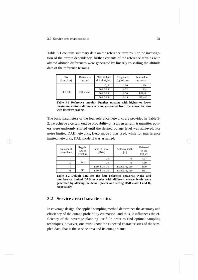
Table 3-1 contains summary data on the reference terrains. For the investiga-tion of the terrain dependency, further variants of the reference terrains withaltered altitude differences were generated by linearly re-scaling the altitudedata of the reference terrains.
The basic parameters of the four reference networks are provided in Table 3-2. To achieve a certain outage probability on a given terrain, transmitter pow-ers were uniformly shifted until the desired outage level was achieved. Fornoise limited DAB networks, DAB mode I was used, while for interferencelimited networks, DAB mode II was assumed.
3.2 Service area characteristics
In coverage design, the applied sampling method determines the accuracy andefficiency of the outage probability estimation, and thus, it influences the ef-ficiency of the coverage planning itself. In order to find optimal samplingtechniques, however, one must know the expected characteristics of the sam-pled data, that is the service area and its outage status.
Size[km x km]
Raster size[m x m]
Max. altitudediff. & σh [m]
Roughness(ρ(10 km))
Referred inthe text as:
100 x 100 250 x 250
0, 0 1.00 flat
300, 52.8 0.32 hilly
300, 52.8 0.50 hilly-L
300, 52.8 0.15 hilly-H
Table 3-1 Reference terrains. Further terrains with higher or lowermaximum altitude differences were generated from the above terrainswith linear re-scaling.
Number oftransmitters
Regularlattice
structure
Emitted Power[dBW]
Antenna height[m]
Referredin the
text as:
7Yes
20 75 G07
19 20 75 G19
9No
mixed: 20, 30 mixed: 75, 150 R09
31 mixed: 20, 30 mixed: 75, 150 R31
Table 3-2 Default data for the four reference networks. Noise andinterference limited DAB networks with different outage levels weregenerated by altering the default power and setting DAB mode I and II,respectively.

32 Outage Probability Estimation
In order to motivate our further discussions, we present a pair of example SIRmaps in Figure 3-1.
The map on the left side was generated over a flat terrain, while the map onthe right side was calculated using our reference hilly terrain. In both cases thetarget area is a circular area over the 100 x 100 km terrain segment with 250 mresolution. The same reference network configuration was used for both cases,and tuned to provide approx. 30% outage, by uniformly shifting the emittedpower of the transmitters. This tuning was carried out separately for the twocases. Comparing the two maps, one can identify that there are two main char-acteristics of the maps:
1 Outage points are often clustered, i.e., the outage status of theneighbor points are often strongly correlated.
2 There are certain points in the service area where outage happenswith higher probability than at other places. This indicates place-dependent probability.
Finding rules of the correlation helps to identify minimal distance betweensampled points (testpoints), and may or may not motivate to use adaptive sam-pling. If apriory rules can be found that can tell us before actual samplingwhere the places with high outage are, this may call for stratified sampling.
Figure 3-1 Example SIR maps for a flat and a hilly terrain by the same out-age probability (30%), using reference network R09, propagation model:Ladell
flat terrain hilly terrain

3.2 Service area characteristics 33
The following two subsections investigate the above two main characteristicsof outage status maps.
3.2.1 Spatial correlation of the coverage
Intuitively, there are four potential factors that affects how much the outagespots on the service area are clustered, such as
1 the applied wave-propagation model,
2 the actual outage probability,
3 terrain characteristics and
4 the network configuration.
This subsection gives an overview of how the spatial correlation of the outagespots can be characterized, investigates the effect of those four factors, andconcludes how the found rules can be used for designing the sampling process.The spatial correlation coefficient is defined by
(3-4)
where
. (3-5)
Figure 3-2 presents the normalized correlation of the outage status as a func-tion of the distance between sampled points, for a number of networkconfigurations and for flat and hilly terrains. There is one apparent commonfeature of the curves, namely that they are decaying in a nearly exponentialfashion. Lets denote z1, z2,..., zi a series of RVs representing the outage statusof consecutive neighboring samples starting from a given point and movingalong a straight line at a constant step, . As before, zi is equal to 1 if point iis not covered, 0 otherwise. If we model the above series via a two-state dis-crete “time” Markov chain, then with properly set state transition probabilitiesp10 and p01, we can mimic the correlation structure of any of the presentedconfigurations quite well. Putting this in the reverse way, the spatial correla-tion of the outage maps can be modeled via a two-parameter model. Since p10and p01 determines together the outage probability itself, which we suppose tobe known, one of the probabilities can be omitted. Somewhat arbitrarily, but
ρzi xi yi,( ) z j x j y j,( ), d( )E ziz j E zi E z j –
σziσz j
⋅-------------------------------------------------------=
d xi x j–( )2 yi y j–( )2+=
θ

34 Outage Probability Estimation
without loosing generality, we chose the complement of p10, γc = p11 = 1 –p10, to describe the size of outage clusters, which can generally be defined viathe following conditional probability in the two-dimensional space:
. (3-6)
Due to the application of digital terrain database with sectorized (rasterized)information of resolution , the conditional probability isdetermined at θ=250m. In the rest of the chapter the symbol γc will coincidewith notation . The following table shows the γc values for thesame cases as presented in the previous figure.
Figure 3-2 Example normalized correlation curves for the outage status vs.the distance between sampled points, propagation model: Ladell
Networkγc
flat hilly
DAB I, G07, 30% outage 0.9721 0.5174
DAB I, G07, 10% outage 0.9373 0.3048
DAB I, G07, 1% outage 0.8957 0.1138
Table 3-3 Conditional probability γc for six example configurations, fordifferent outage levels for flat and hilly terrains.
0 5 10 15 20 25 30 35 400
0.1
0.2
0.3
0.4
0.5
0.6
0.7
0.8
0.9
1
Distance, d [x 250 m]
ρ(d)
Outage probability:po = 0.3po = 0.1po = 0.01
Network:G07, DAB I, flatG07, DAB II, flatG07, DAB I, hilly
γc θ( ) Pr z xi yi,( ) 1= z x j y j,( ) 1= i j– 1=, ≡
250m 250m× γc θ( )
γc θ 250m=( )
3.2 Service area characteristics 35
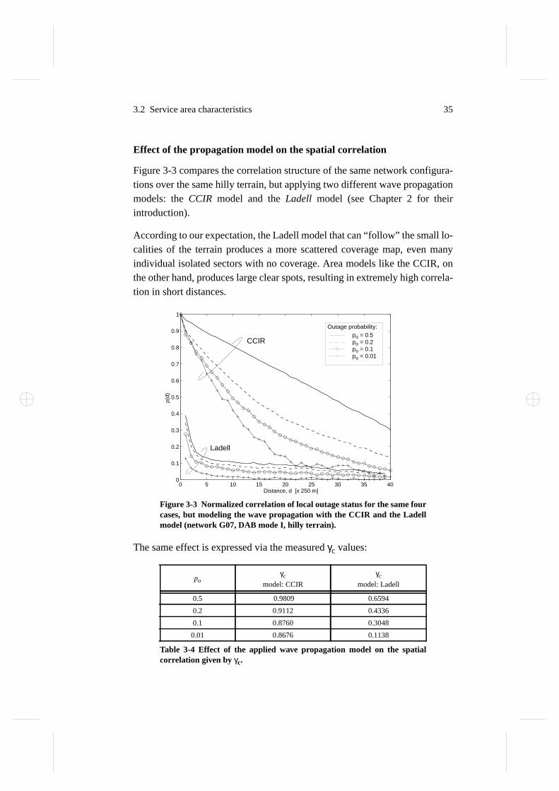
Effect of the propagation model on the spatial correlation
Figure 3-3 compares the correlation structure of the same network configura-tions over the same hilly terrain, but applying two different wave propagationmodels: the CCIR model and the Ladell model (see Chapter 2 for theirintroduction).
According to our expectation, the Ladell model that can “follow” the small lo-calities of the terrain produces a more scattered coverage map, even manyindividual isolated sectors with no coverage. Area models like the CCIR, onthe other hand, produces large clear spots, resulting in extremely high correla-tion in short distances.
The same effect is expressed via the measured γc values:
Figure 3-3 Normalized correlation of local outage status for the same fourcases, but modeling the wave propagation with the CCIR and the Ladellmodel (network G07, DAB mode I, hilly terrain).
poγc
model: CCIR
γc
model: Ladell
0.5 0.9809 0.6594
0.2 0.9112 0.4336
0.1 0.8760 0.3048
0.01 0.8676 0.1138
Table 3-4 Effect of the applied wave propagation model on the spatialcorrelation given by γc.
0 5 10 15 20 25 30 35 400
0.1
0.2
0.3
0.4
0.5
0.6
0.7
0.8
0.9
1
Distance, d [x 250 m]
ρ(d)
Ladell
CCIR
Outage probability:po = 0.5po = 0.2po = 0.1po = 0.01

36 Outage Probability Estimation
Effect of the outage probability on the spatial correlation
It is expected that the clustered feature of the outage spots diminishes with de-creasing outage probability. To verify our expectations, five networkconfigurations have been tuned by power shifting to provide different levelsof outage over the flat and the hilly terrain, and γc values were evaluated. Fig-ure 3-4 presents the result.
Surprisingly, it can be observed that γc does not strongly depend on the net-work configurations, but more clearly affected by the terrain and the outageprobability (the latter two can be intuitively conceived).
Effect of the terrain characteristics on the spatial correlation
To describe the characteristics of the terrain, there are several different param-eters suggested in the literature [2]. One of the simplest way to characterize theundulation and the roughness of the terrain is via the standard deviation ofheights σh and the correlation coefficient between terrain altitudes ρ(d) at oneor more constant distances. In [25] it is shown that natural terrains show nearlyexponentially decaying correlation as a function of d, therefore we assume thatσh and ρ(d = 10 km) determine together the characteristics of the terrain. Ter-rains with different height standard deviations σh and correlation coefficients
Figure 3-4 γc vs. the outage probability for five different network configu-rations over the flat and the hilly terrain, propagation model: Ladell
10−4
10−3
10−2
10−1
100
0
0.2
0.4
0.6
0.8
1
po
γ c
flat
hilly

3.2 Service area characteristics 37
ρ(10 km) have been investigated. Reference network R09 with DAB mode Ihave been adjusted for each test terrain to provide the specified outage proba-bility. Figure 3-5 presents the resulted correlation expressed via the respectiveγc for outage level .
It can be seen that γc decreases very steeply in the range of σh ~ 0-30 m, anddeviations larger than 50 m have no considerable further effect. The impact ofthe terrain correlation seems to be independent of the deviation, giving a near-ly constant shift to γc values.
So far, we have investigated the correlation characteristics of coverage maps.We have seen that γc depends strongly on the applied propagation model. Thefigures showed that the very low outage yields low correlation. Obviously, flatterrain gives higher correlation than hilly terrain. The correlation of the cover-age for flat terrain decreases slowly with decreasing outage level. On the otherhand, for hilly terrain the correlation decreases steeply with decreasing outagedue to terrain irregularities. The terrain is the most important factor that effectsthe correlation, while the actual network structure has negligible effect.
We characterized the spatial correlation of the outage by parameter γc. We canestimate the average radius of the outage clusters rc = as to satisfythe equation , where ν is a constant (e.g. ν = 0.5). To achieve effi-
Figure 3-5 γc versus terrain altitude standard deviation σh, for three differ-ently autocorrelated terrains. po= 0.1, propagation model: Ladell
po 0.1=
ρ(10km) = 0.15
ρ(10km) = 0.32
ρ(10km) = 0.5
0 50 100 150 200 2500.2
0.3
0.4
0.5
0.6
0.7
0.8
σh [m]
γ c
k 250m×γc( )k ν=

38 Outage Probability Estimation
cient outage estimation, the distance [m] can be used as aminimal distance between testpoints.
3.2.2 Location dependency of the outage
The other potential way of improving the efficiency of the outage probabilityestimation is to find some location-dependent variables external to the sam-pling process that show high correlation with the local outage status. If such avariable could be found, it would call for stratified sampling. There are two in-tuitively apparent sources for such a variable, such as:
• the altitude at the terrain element,
• the relative position of the terrain element within the transmitternetwork.
In the following sub-sections we investigate those two sources.
Dependency of the outage on terrain altitudes
The dependency of the local outage status on the terrain altitude is investigatedin the following way: the entire set A of all terrain elements within the targetservice area is divided into non-overlapping sub-sets (strata)according to their altitude, and the following conditional probability
is determined for strata k.
The above investigation has been carried out for a number of different networkconfigurations. Figure 3-6 to 3-7 summarizes our results. Figure 3-6 showsthree cases where noise limited DAB networks (mode I) were set to achievepo = 0.01, 0.1, 0.3 outage probabilities. The strata have been defined by di-viding the entire altitude range of the terrain into mh = 10 equal sub-ranges.The vertical axis shows the conditional probabilities per stratum normalizedto the overall outage probability.
The results show that, for the investigated networks, most of the outage hap-pened at the two strata with the lowest altitude, and almost zero outage wasobserved at the four highest strata. This result is reasonable since we could ex-pect that when the SNR is the limiting factor, then points located at low altitudeand potentially shielded by terrain obstacles are the most sensitive one.
dmin 2k 250×≤
A1h
A2h ... Amh
h, , ,
po k( ) Pr zi j, 1= zi j, Akh∈( ) =

3.2 Service area characteristics 39
Figure 3-7 presents two cases where DAB with mode II was applied. It can be
Figure 3-6 Normalized outage probability per altitude-based terrain stra-tum for DAB mode I (noise limited case). Propagation model: Ladell.a: outage probability 0.3b: outage probability 0.1c: outage probability 0.01
Figure 3-7 Normalized outage probability per altitude-based terrain stra-tum for DAB mode II (interference limited). Propagation model: Ladella: outage probability 0.3b: outage probability 0.1
1 2 3 4 5 6 7 8 9 100
0.5
1
1.5
2
2.5
3
Height strata
p o (
stra
tum
) / p
o
a
b
c
1 2 3 4 5 6 7 8 9 100
1
2
3
4
5
6
7
Height strata
p o (
stra
tum
) / p
o
a
b

40 Outage Probability Estimation
seen that moving from a noise limited environment to an interference-limitedone can smooth down this distribution or even reverse the situation: nowpoints at the highest altitude become the most vulnerable ones. It can be intu-itively explained such that the probability that a point is visible by both theuseful and the interfering transmitters is increasing with increasing altitude.
It can be concluded from the above results that if the presence of interferencecan be excluded from a certain design case e.g. when DAB mode I is appliedover a relatively small service area, we can confidently say that uncoveredpoints are located at low altitudes. In these cases stratified sampling might beworthwhile to apply. However, in the case of unknown interference situation,we can say nearly nothing about the expected place of outages.
Dependency of the outage on the network configuration
The other potential source for apriori knowledge on the local outage is the po-sition of the area element relative to the transmitters in the network. Weformulate our control variable d for the area element as follows: for each trans-mitter that submits signal to the receiver at the area element with coordinates(xa, ya), we determine the relative distances between (xa, ya) and the transmit-ter (xt, yt), as the true distance normalized to the noise limited coverage radius(Ro) of the transmitter assuming flat terrain. The shortest relative distance ischosen to formulate our strata.
Figure 3-8 shows the results for DAB network. The probability of outage isincreasing with the increasing relative distance from the transmitters. Similar-ly to the previous sub-section, in the case of interference, the outage level canincrease considerably in the near vicinity of the transmitters, compared to thenoise-limited cases.
The results indicate that it is relatively safe to say that the majority of the un-covered points are located farther from the transmitters than the 75% of thenoise limited coverage radius.
3.3 Sampling techniques
In the preceding part of the chapter we studied the basic characteristics of net-work coverage status maps and now we are ready to overview the possible

3.3 Sampling techniques 41
sampling strategies to suggest efficient methods for outage probabilityestimation.
An ordered sample of size n is sequence s0 = ((i1, j1),....., (in,jn)) of n of thearea elements. The set of the possible samples is denoted by S0. The samplingdesign may be specified as a conditional probability of select-ing the sample so for each possible sample of . The selectionprobabilities may depend on any observations of the variable of interest z oron any auxiliary variable v.
In a conventional design, the selection probabilities do not depend on any ob-servations of the variable of interest z, therefore the entire sample may beselected prior to the survey. However, they may depend on any auxiliary vari-able v known for the population. In the thesis a number of conventionalsampling surveys will be investigated such as the simple random samplingwithout replacement, stratified random sampling based on terrain, stratifiedrandom sampling based on the network configuration and systematicsampling.
In adaptive sampling the procedure of selecting units may depend on values of
Figure 3-8 Probability of outage versus of normalized distance from thetransmitter, system: DAB, propagation model: Ladell1a: po = 0.3, noise limited 2a: po = 0.3, interference limited1b: po = 0.1, noise limited 2b: po = 0.1, interference limited1c: po = 0.01,noise limited
0 0.5 1 1.50
0.1
0.2
0.3
0.4
0.5
Normalized distance from transmitter, r / Ro
Loca
l out
age
prob
abili
ty
1a
1b
1c
2a
2b
Pr s0 z v,( ) s0 S0∈

42 Outage Probability Estimation
the variable of interest, but only through units included in the sample duringthe survey, i.e. . Thus, the sampling plan has the flex-ibility to change during the survey in response to observed patterns. Theapplication of this type of sampling to our problem will not be discussed in thisthesis, but it is suggested for future research [27].
3.3.1 Simple random sampling
Simple random sampling (SRS) is a method of selecting n elements at randomout of nA such that all elements have an equal chance of being included in thesample. In practice SRS is drawn element by element. The applied samplingis without replacement, i.e. the selected sample is not replaced into the popu-lation. The sample mean zsrs of z is an unbiased and consistent point estimateof po:
(3-7)
We select independently n elements at random —so that all elements have anequal chance of being included in the sample— without replacement andcount the number of “outage”-elements (q) in our sample. q is a RV and has ahypergeometric distribution H(nA, n, po):
(3-8)
(k takes on all integer values such that ).For a hypergeometric distribution we have
(3-9)
The mean is the same as for the binomial distribution, but the variance is dif-ferent. There is a factor in the hypergeometric case,and it is called the finite population correction. If nA is large compared to n,the RV q is approximately binomially distributed (Bin(n, po)) and dn is near to1, otherwise the variance of the hypergeometric distribution is less than thevariance of the binomial distribution.
Pr s0 z Pr s0 zs0 =
zsrs1n--- zi
i 1=
n
∑= where η zsrspo= and σzsrs
2E zsrs po–( )2 =
pq k( )nA po
k nA 1 po–( )
n k– nA
n ⁄=
0 k nA po≤ ≤ 0 n k– nA 1 po–( )≤ ≤,
E q n po=
σq2 nA n–
nA 1–---------------n po 1 po–( )=
dn2 nA n–( ) nA 1–( )⁄=

3.3 Sampling techniques 43
Confidence interval estimation
Our interest is to consider the relative error (ε). As an intermediate step wedetermine the relative frequency of “outage”, that is, the ratio z = q/n of thefrequency to the total number of trials. The distribution of z is easily obtainedfrom that of q:
(3-10)
Our goal is to minimize the relative error , which has the dis-tribution from that of z.
(3-11)
For large n the distribution of ε is approximately ~ N(0, ). Hence
(3-12)
The is the α/2-quantile of a standard normal distribution N(0,1). Forlarge n the following approximation can be used to obtain the confidence in-terval, if we replace on the right side the unknown po by its point estimate z:
(3-13)
The interval Iε covers ε with probability , called confidence level.If n/nA is smaller than 0.1, we may take dn = 1, without introducing any seriouserror. Let us examine how the length of the interval depends on the size of nA
of the population and the size of n. For a given confidence level the intervallength is determined as:
(3-14)
From (3-14) it follows, that for satisfying a given confidence interval length:
(3-15)
E z po σz2
dn2po 1 po–( ) n⁄=;=
ε z po–( ) po⁄=
E ε 0; σε σz po⁄ dn
1 po–( )n po
-------------------= = =
σε2
P ε λα 2⁄ σε< γ 1 α–= =
λα 2⁄
Iε λα 2⁄ d– λα 2⁄ d,( ) where d dn1 z–( )nz
----------------==
1 α–
L λα 2⁄nA n–( )nA 1–( )
------------------- 1 z–( )nz
----------------=
n ∆2 1nA------+
1–where ∆ L
λα 2⁄----------- z
1 z–( )----------------=>
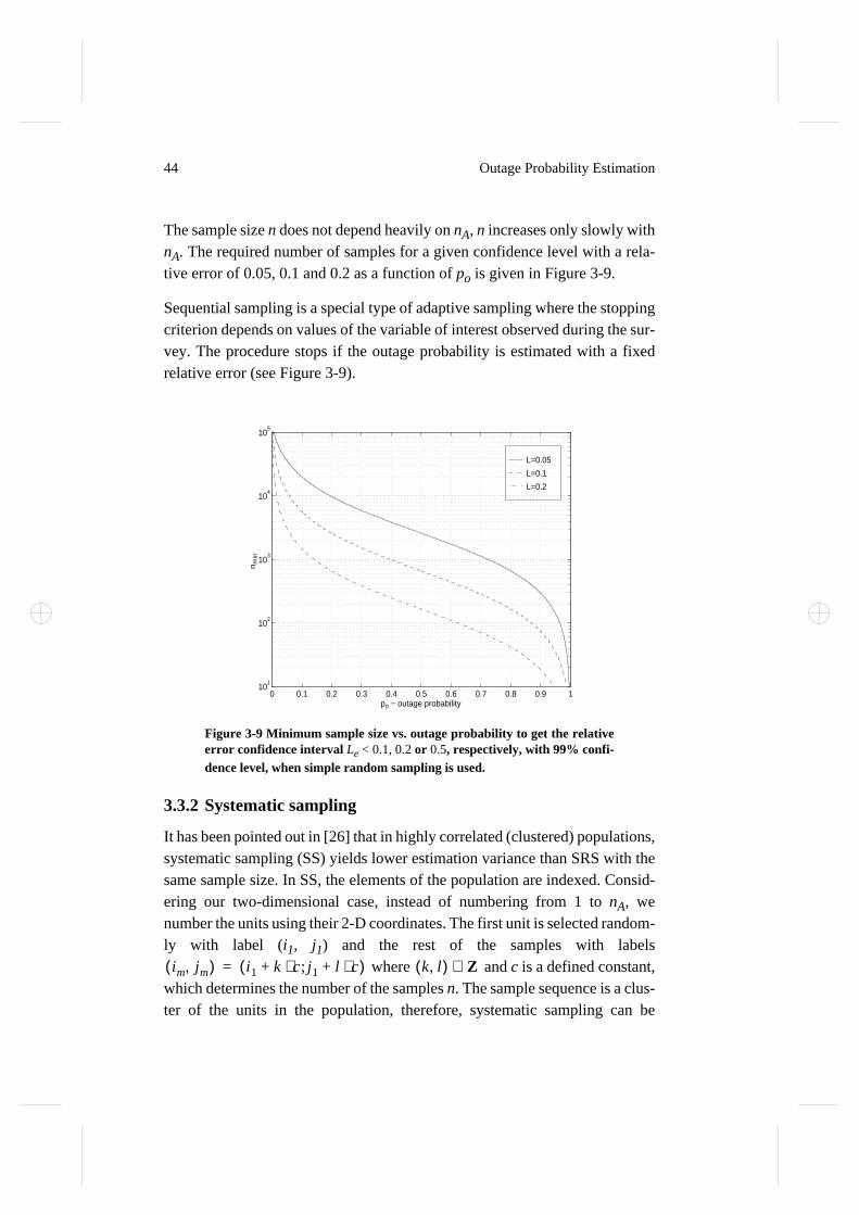
44 Outage Probability Estimation
The sample size n does not depend heavily on nA, n increases only slowly withnA. The required number of samples for a given confidence level with a rela-tive error of 0.05, 0.1 and 0.2 as a function of po is given in Figure 3-9.
Sequential sampling is a special type of adaptive sampling where the stoppingcriterion depends on values of the variable of interest observed during the sur-vey. The procedure stops if the outage probability is estimated with a fixedrelative error (see Figure 3-9).
3.3.2 Systematic sampling
It has been pointed out in [26] that in highly correlated (clustered) populations,systematic sampling (SS) yields lower estimation variance than SRS with thesame sample size. In SS, the elements of the population are indexed. Consid-ering our two-dimensional case, instead of numbering from 1 to nA, wenumber the units using their 2-D coordinates. The first unit is selected random-ly with label (i1, j1) and the rest of the samples with labels
where and c is a defined constant,which determines the number of the samples n. The sample sequence is a clus-ter of the units in the population, therefore, systematic sampling can be
Figure 3-9 Minimum sample size vs. outage probability to get the relativeerror confidence interval Le < 0.1, 0.2 or 0.5, respectively, with 99% confi-dence level, when simple random sampling is used.
L=0.05
L=0.1
L=0.2
0 0.1 0.2 0.3 0.4 0.5 0.6 0.7 0.8 0.9 110
1
102
103
104
105
po − outage probability
nm
in
im jm,( ) i1 k c⋅+ j1 l c⋅+;( )= k l,( ) Z∈

3.3 Sampling techniques 45
considered as a simple random sampling applied to a set of clusters with setsize c2. The size of the clusters may be different, which may introduce somedisturbance, but for our cases where n > 50, it can be ignored. The point esti-mate of systematic sampling coincides with eq. (3-7).
3.3.3 Stratified sampling
In stratified sampling (STS) the population A of nA units is divided into sub-populations A1, A2,...,AL of N1, N2,..., NL units, respectively. Thesesubpopulations called strata are non-overlapping and they comprise the wholepopulation nA = N1 + N2 +... + NL. For the population unit mean per unit, thesimplest type of estimate appropriate to stratified sampling is zsts [26],
(3-16)
where the following symbols refer to the stratum h: Nh is the total number ofunits, nh number of units in the sample, zhi is the value of the ith unit and zh isthe sample mean of the stratum h. L is the number of strata.
The basic idea behind stratified sampling is, that it may bring a gain in preci-sion in the estimates of characteristics of the whole population dividing theheterogeneous population into internally homogeneous sub-populations. Thevariance of the estimated mean zsts is smallest, if the sample is allocated withnh proportional to Nhσh.
According to the results of the previous sub-section, we will apply stratifiedsampling on the basis of two auxiliary variables: At first, the strata will be de-fined based on the terrain characteristics (T-STS) — more precisely, thealtitude information of terrain sectors will form our stratification variable.
Secondly, stratified sampling will be investigated based on network configu-ration (N-STS). Our assumption is that receivers in the vicinity of thetransmitters are safe against coverage outage, the intersection areas are moreexposed to low coverage probability.
zsts1
nA------ Nh zh⋅
h 1=
L
∑= where zh1nh----- zhi
i 1=
nh
∑=
46 Outage Probability Estimation
3.4 Numerical results
So far in this chapter we studied the basic characteristics of outage status mapsfor SFNs, and we have investigated some of the sampling methods that can beapplied for efficient outage probability estimation.
The performance of the sampling methods have been evaluated on a largenumber of test networks, in terms of their required sample size to achieve agiven confidence level. Figures 3-10 and 3-11 contain an extraction from ourresults, where the following four sampling algorithms have been applied to theG09 reference network with outage level po = 0.1 and both for flat and for hillyterrains:
• Simple random sampling (SRS)
• Systematic sampling (SS)
• Network-based Stratified Sampling (N-STS) with two strata
• Terrain-based Stratified Sampling (T-STS), only for cases with the hillyterrain with two strata.
Their performance is presented as the relative error with 99% confidence levelas a function of the sample size n.
In general, it can be seen that SRS had the poorest performance, we present ithere mainly for the sake of comparison. It is also apparent from the figures thatsystematic sampling came out as the best in most of the cases, outperformingboth the network-based and the terrain-based stratified simple random sam-pling methods, although its advantage is slighter on hilly terrains (see Figure3-11), where the spatial correlation of the outage status is negligible.
The relatively week performance of both stratified sampling methods can beexplained by the fact that the sampled variables are in our case binary vari-ables: The sampling gain (i.e. the variance reduction) of stratified samplingcan be considerable only if there can be found a stratum (or a few of them)with relatively small population but with much higher variance than in the restof the sampling space. In our case, the sampled RV:s are binary, so the samplevariance is ranged between 0 and 0.5. Large variance differences would occuronly if one could find strata with variance near to 0, which would require ex-tremely small outage probability in the given stratum. In practical cases, it isvery unrealistic to find such a stratum.

3.4 Numerical results 47
Figure 3-10 Coefficient of variance vs. number of samples;Parameters: po = 0.10; flat terrain, propagation model: Ladell
Figure 3-11 Coefficient of variance vs. number of samples;Parameters: po = 0.10; hilly terrain, propagation model: Ladell
SRS
SS
N−STS
102
103
104
105
10−3
10−2
10−1
100
101
n − number of samples
L −
co
nfid
en
ce in
terv
al l
en
gth
Flat terrain, Outage: 0.100000
SRS
SS
N−STS
T−STS
102
103
104
105
10−3
10−2
10−1
100
101
Hilly terrain, Outage: 0.100000
n − number of samples
L −
co
nfid
en
ce in
terv
al l
en
gth
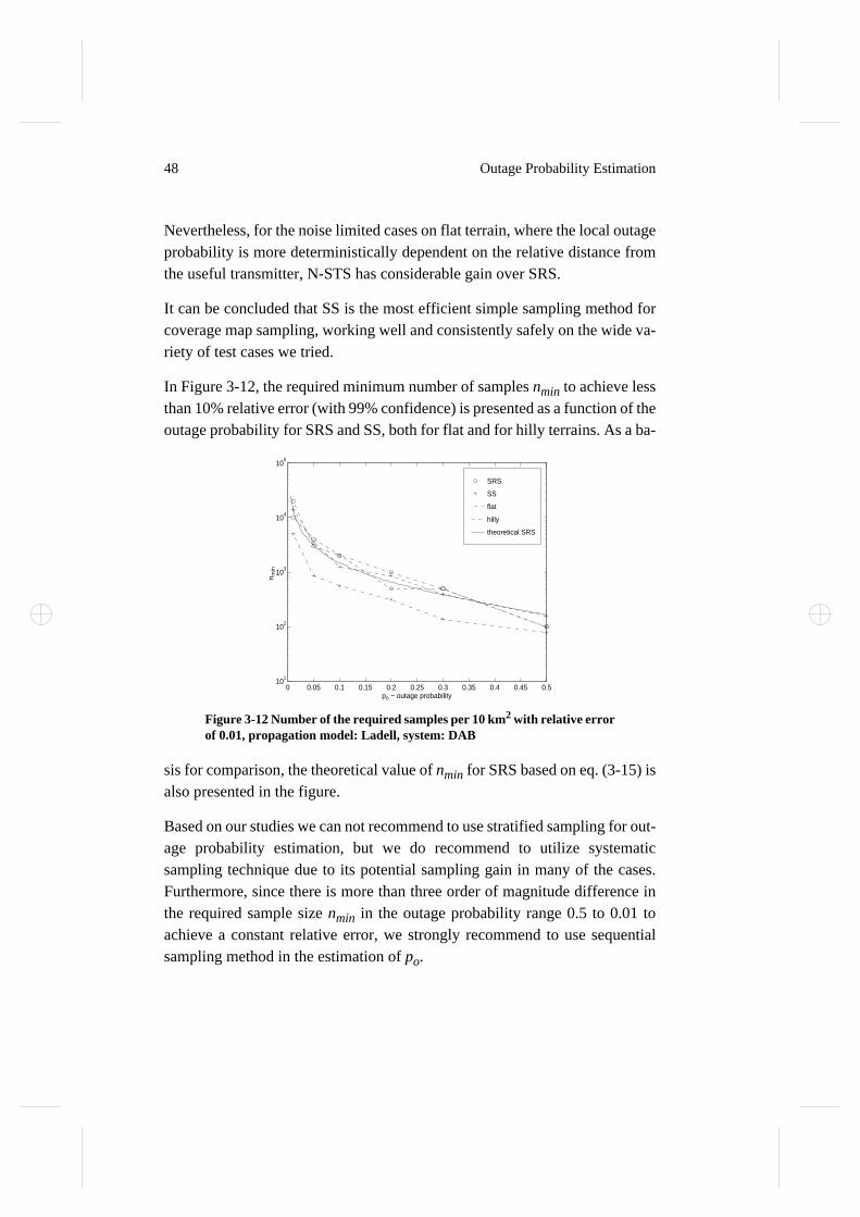
48 Outage Probability Estimation
Nevertheless, for the noise limited cases on flat terrain, where the local outageprobability is more deterministically dependent on the relative distance fromthe useful transmitter, N-STS has considerable gain over SRS.
It can be concluded that SS is the most efficient simple sampling method forcoverage map sampling, working well and consistently safely on the wide va-riety of test cases we tried.
In Figure 3-12, the required minimum number of samples nmin to achieve lessthan 10% relative error (with 99% confidence) is presented as a function of theoutage probability for SRS and SS, both for flat and for hilly terrains. As a ba-
sis for comparison, the theoretical value of nmin for SRS based on eq. (3-15) isalso presented in the figure.
Based on our studies we can not recommend to use stratified sampling for out-age probability estimation, but we do recommend to utilize systematicsampling technique due to its potential sampling gain in many of the cases.Furthermore, since there is more than three order of magnitude difference inthe required sample size nmin in the outage probability range 0.5 to 0.01 toachieve a constant relative error, we strongly recommend to use sequentialsampling method in the estimation of po.
Figure 3-12 Number of the required samples per 10 km2 with relative errorof 0.01, propagation model: Ladell, system: DAB
SRS
SS
flat
hilly
theoretical SRS
0 0.05 0.1 0.15 0.2 0.25 0.3 0.35 0.4 0.45 0.510
1
102
103
104
105
po − outage probability
nm
in

49
Chapter 4
Minimal Cost Coverage Planningfor SFN based DAB
There are many aspects that have to be considered during coverage planningof radio networks. Some of the most important factors are: quality of the cov-erage, size of the service area, cost of implementation and provisioning,coordination with existing networks (generated interference) and frequencyreuse factor. Depending on how these and other factors are incorporated intothe design, there can be many possible strategies. When optimization is in-volved in the design, each of these factors can be either part of the objectivefunction or subject of certain constraints or neglected in the optimization pro-cess. Our formulation of the optimization problem involves all of the abovefactors except frequency reuse, although the latter could also be taken into ac-count with a straightforward extension of the model.
Contrary to FM coverage planning, — where the focus is on the frequency as-signment, and the rest of the parameters are often disregarded from theoptimization (fixed values) — the frequency planning becomes a secondaryproblem in SFN’s. The main issue is the delay planning with optimization ofthe transmitter parameters such as transmitter location, transmitted power, an-tenna height, antenna diagram and temporal broadcasting delay (or offset), allof which can be individually assigned to each transmitter. The total number oftransmitters is also a free parameter.
The transmitter parameters can be divided into the classes of discrete and con-tinuous parameters: Frequency assignment is usually formulated as a purelydiscrete problem. Some of the parameters (antenna height, power, location)are continuous, but in the practice some of them are handled often in a discreteway. The locations of transmitters are usually considered to be discrete due toutilization of existing available antenna towers, of which reuse can consider-ably decrease the cost of the network. In this case there are also some

50 Minimal Cost Coverage Planning for SFN based DAB
limitations on the antenna height depending on the tower height and the occu-pancy of the tower by other services.
In our optimization problem the location, transmitted power, antenna heightare the decision variables given by discrete sets. The number of transmitters isalso a decision variable. The frequency allotment plan for national and region-al programs has been already determined for the European countries [49], sowe assume that the frequency of the SFN is already given. The antenna pat-terns are assumed omnidirectional and the transmitters are simulcasting, i.e.there is no temporal offset applied. The objective function includes the qualitymeasure of the coverage of the new service over the predefined service area,the network hardware cost and the maximum allowable generated interferencelevel. The effect of the existing networks on the service area of the new DABservice is included in the quality measure.
Coordination with the existing networks (by controlling the generated interfer-ence), can be performed during the optimization, or after the optimizationusing the algorithm suggested in [65]. There, the authors describe a coordina-tion process which checks the interfering total fieldstrength created by the newnetwork at coordination testpoints located outside the service area at a pre-defined distance from the network. If the interfering fieldstrength exceeds theallowable predefined value, antenna pattern correction of the transmitters nearto the edges of the service area is applied. These predefined coordination pa-rameters are specified in [49] for each DAB frequency band.
Our problem is a planning problem (as opposed to a real-time control prob-lem); it is not required to solve it in a very short time. To design the coveragefor a new network, the time that is available to obtain the solution can be as-sumed from some days to some months. In practical planning we have tohandle particular problem with its given state space. In smaller problems evenexhaustive search can be a feasible approach, while larger networks would re-quire hundreds of years to find the globally optimum solution. Knowing thescale of the problem, appropriate optimization techniques have to be selected.
Our problem is not tractable analytically. Reliable propagation predictionmodels are based on sophisticated calculations involving topographical data.The summation of log-normal variables in calculation of the total fieldstrengthis built on the basis of statistics. For determining the coverage probability for
4.1 Objective function and state space 51
each terrain element we have to calculate the constructive or interfering con-tribution of each transmitter. This status varies from terrain elements to terrainelements. The outage probability is computed using a discrete estimate, wherethe estimation error is induced by the terrain database quantization, propaga-tion model and the applied sampling technique. Consequently, we optimizethe sample outage of one realization of the testpoint selection. The objectivefunction is a weighted sum of the sample outage and the cost function. Wehave to face a nonlinear discrete function with high-dimensionality, which re-sults in a non-linear discrete optimization problem.
There have been other attempts to optimize the coverage of SFNs. For in-stance, authors of [64] present a method that maximizes the size of thecoverage area, satisfying a given quality constraint. Up to our knowledge, ourwork is novel in the sense that it involves cost and external interference issuesin the optimization.
For solving such an optimization problem we apply heuristic and stochasticoptimization techniques. The detailed description of the methods is given inthe next sections. Our goal is twofold: the one hand to suggest effective algo-rithms for network planning, on the other hand to discover inherent features ofSFN transmitter configurations with the help of optimization. The rest of thischapter deals with the first issue, the second one is treated by Chapter 5.
4.1 Objective function and state space
In order to derive an optimization problem with a discrete state space, thetransmitter parameters are confined to discrete parameters. The radiated pow-er, antenna height and transmitter location may take values from the “feasible”sets:
(4-1)
The , and denote the size of the respective sets. These feasible setsare defined for all transmitter sites uniformly, and each transmitter can chooseany of the values from the sets. A more practical extension of this model
S S1 S2 … SnS, , , =
P P1 P2 … PnP, , , =
H H1 H2 … HnH, , , =
nP nH nS

52 Minimal Cost Coverage Planning for SFN based DAB
would be the case where the power and antenna height sets were defined indi-vidually for each transmitter location. Though we restricted our formulation tothe uniform case, the presented techniques can be applied to the more generalformulation in a straight forward manner.
The design objective is defined as follows:
minimize
subject to and (4-2)
for
where
,
,
, , and . (4-3)
The penalty method [31] is applied to approximate the constrained optimiza-tion problem given by (4-2) by an unconstrained problem. The approximationis accomplished by adding a term to the objective function that prescribes ahigh cost if the constraint is violated. The unconstrained optimization problemis formulated as:
minimize (4-4)
where the network cost is normalized to an externally given “ceiling” cost(Cmax). The penalty for violating the coverage requirement is given by equa-tion (4-5).
(4-5)
is the penalty for violating the generated interferencelimit, where n*K is the number of coordination testpoints where the constraintis not satisfied. Parameters α, β and γ are external constants that determine theseverity of the penalties.
CN N( )
po N I,( ) po max,<
EU N ki,( ) EU max,< ki K∈
N t1 t2 ... tnN, , , Ω∈=
ti pi hi si, ,⟨ ⟩=
pi P∈ hi H∈ si S∈ nN Z+∈
f N( ) CN N( ) Cmax⁄ χC N I,( ) χI N K,( )+ +=
χC N I,( )α
po N I,( ) po max,–
1 po max,–------------------------------------------⋅ β+ po N I,( ) po max,≥
0 po N I,( ) po max,<
=
χI N K,( ) γ n∗ K⋅=

4.2 Algorithms 53
Considering new transmitters, the set of possible network configurations(Ω) of the design problem has the size of
, (4-6)
provided that not more than one transmitter can be placed at a single site. If wealso let nN be a decision variable, the total state space becomes
. (4-7)
Concerning the cost of the network, we apply the following simplified model:For each value of set P, H and S a relative cost value is defined. CP, CH andCS denote the sets of cost values associated to P, H and S, respectively. If atransmitter i uses the power quantity step k from P, antenna height step l fromH and site m from S, its cost is calculated simply as .
4.2 Algorithms
All exact methods known for determining the global optimal solution for NPcomplete problems require a computing time that increases exponentially inthe worst case as the problem size increases. We will apply an exact method(deterministic total search, TS) to determine the optimal solution for small-scale problems and to provide a basis for comparison when measuring the per-formance of other heuristic algorithms.
Real life problems only seldom require the global optimum, a suboptimal so-lution can already be satisfactory, provided a certain evidence that it is not toobad. In practical problems, approximative heuristic approaches designed withgood engineering sense, exploiting the inherent feature of the specific problemin hand can give surprisingly good performance, although, they may sacrificethe guarantee of optimality — or in case of constrained problems even theguarantee that a satisfactory solution is found. Preferred heuristic methods arethose that bear polynomial running time and memory requirements.
Stochastic searching techniques such as Simulated Annealing (SA) (due toKirkpatric, Gelatt and Vecchi [34]), are another source of tools to successfullyattack NP compete problems.
nN
ℑ Ω nN( ) nPnH( )nNnS!
nS nN–( )! nN!⋅-------------------------------------=
ℑ Ω nPnH 1+( )nS 1–=
Ct ti( ) CkP
ClH
CmS+ +=

54 Minimal Cost Coverage Planning for SFN based DAB
Stochastic and heuristic elements can be combined into one searching algo-rithm, which can further improve efficiency, via compensating the shortage ofthe involved specific elements. Two possible ways for the integration are: (1)hybrid techniques that utilize both elements in the same time, or (2) multi-stage optimization algorithms where stochastic and heuristic elements are ap-plied sequentially to solve the same problem. Examples for hybrid methodsare when randomness is involved in a heuristic search or when heuristic ruleshelp SA to determine the next state during its stochastic search. Multi-stagetechniques can be best exemplified via a method that uses a simple heuristicalgorithm to find an “initial” state from which stochastic SA can start search-ing for further improvements.
In the following subsections we introduce three basic algorithms that havebeen developed to serve as a basic component in solving our coverage plan-ning problem. Two of them are hybrid methods: the first one is a constructivemethod that builds a network from scratch in a sequential (step-by-step) man-ner, using heuristic rules. The second algorithm implements a localtransformation method that aims to improve an existing solution by (local-)searching a well defined neighborhood of the original solution. Both applyrandomness in the searching process. Our third algorithm is a special adapta-tion of the general SA to our coverage planning problem.
In Section 1 we mentioned a number of references in the literature where au-thors applied stochastic or heuristic algorithms to coverage planning in radionetwork design. The main importance of our work comes from the very prac-tical but still compact formulation of the problem i.e. incorporating theinternal and external interference constraints and cost aspects into a non-con-strained optimization problem. The applicability of known heuristic searchingtechniques to this type of problem formulation was unknown. A further nov-elty of our work is the set of basic searching algorithms specifically developedor tailored to the above problem, moreover, a number of multi-stage algo-rithms constructed from the basic components to efficiently solve the SFNcoverage design problem.
In all the three methods, randomness plays an important role. In the definitionsof the algorithms “randomly chosen” means “randomly chosen with uniformdistribution”, if not specifically stated.
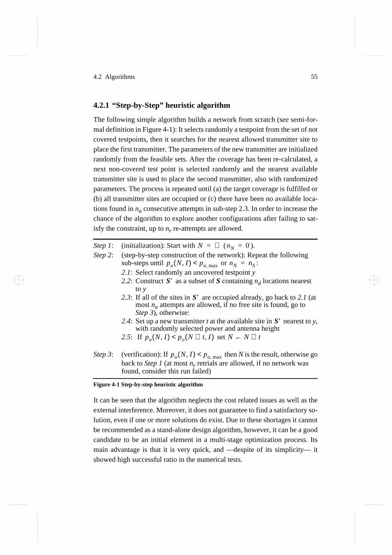
4.2 Algorithms 55
4.2.1 “Step-by-Step” heuristic algorithm
The following simple algorithm builds a network from scratch (see semi-for-mal definition in Figure 4-1): It selects randomly a testpoint from the set of notcovered testpoints, then it searches for the nearest allowed transmitter site toplace the first transmitter. The parameters of the new transmitter are initializedrandomly from the feasible sets. After the coverage has been re-calculated, anext non-covered test point is selected randomly and the nearest availabletransmitter site is used to place the second transmitter, also with randomizedparameters. The process is repeated until (a) the target coverage is fulfilled or(b) all transmitter sites are occupied or (c) there have been no available loca-tions found in na consecutive attempts in sub-step 2.3. In order to increase thechance of the algorithm to explore another configurations after failing to sat-isfy the constraint, up to nr re-attempts are allowed.
It can be seen that the algorithm neglects the cost related issues as well as theexternal interference. Moreover, it does not guarantee to find a satisfactory so-lution, even if one or more solutions do exist. Due to these shortages it cannotbe recommended as a stand-alone design algorithm, however, it can be a goodcandidate to be an initial element in a multi-stage optimization process. Itsmain advantage is that it is very quick, and —despite of its simplicity— itshowed high successful ratio in the numerical tests.
Step 1: (initialization): Start with ( ).Step 2: (step-by-step construction of the network): Repeat the following
sub-steps until or :2.1: Select randomly an uncovered testpoint y2.2: Construct as a subset of S containing nd locations nearest
to y2.3: If all of the sites in are occupied already, go back to 2.1 (at
most na attempts are allowed, if no free site is found, go toStep 3), otherwise:
2.4: Set up a new transmitter t at the available site in nearest to y,with randomly selected power and antenna height
2.5: If set
Step 3: (verification): If then N is the result, otherwise goback to Step 1 (at most nr retrials are allowed, if no network wasfound, consider this run failed)
Figure 4-1 Step-by-step heuristic algorithm
N ∅= nN 0=
po N I,( ) po max,< nN nS=
S ′
S ′
S ′
po N I,( ) po N t∪ I,( )< N N t∪←
po N I,( ) po max,<

56 Minimal Cost Coverage Planning for SFN based DAB
4.2.2 Local search
One obvious possibility to further optimize the solution found by the step-by-step method is to apply a local search method that aims to improve the existingsolution by locally searching a well-defined neighborhood of the given solu-tion. A Local Search (LS) algorithm that is specifically formulated to workwith our model is presented in Figure 4-2, and it works as follows: During oneiteration of the searching process it “visits” each of the transmitters once, ac-cording to a random order. (The order of visits is randomized individually foreach iteration in Step 1.) During visiting a transmitter the algorithm tries tomodify the power and antenna height parameters of the transmitter in order todecrease the objective function, that is, either improving the coverage or low-ering the total cost of the network. As an extreme case, the algorithm can eveneliminate (switch off) a transmitter temporarily if that is justified by the objec-tive function. In a later iteration, such a transmitter can be re-activated(switched on) by assigning the lowest power and antenna height value from thefeasible set. However, if a transmitter is found to be switched off at the end ofthe searching process, it is removed from the solution set. If no improvementcan be found, the parameter is left intact. The iterations are repeated until nofurther improvements have been made within the last iteration.
According to the “greediness” of a single visit, two variations of the schemeexist: (1) during one visit each parameter is allowed to be shifted only to thenext higher or next lower value of the feasible set (non-greedy), or (2) the bestpossible value in the feasible set (in terms of the impact to the objective func-tion) is searched for and assigned at each visit for each parameter (greedy).From now on we denote greedy and non-greedy variation of LS by LSG andLSN, respectively.
The algorithm is strictly monotonous in the sense that only improvements areallowed. Consequently, provided that the initial solution is feasible (i.e. theconstraints in (4-2) are not satisfied), the result remains always feasible, al-though it might be far away from the global optimum.
The same searching scheme can be applied to randomly generated configura-tions, though the result is not guaranteed to be feasible in such cases. Underrandom initial configuration we mean a network where a randomly selectedsubset of the available transmitter locations are planted by randomly parame-

4.2 Algorithms 57
terized transmitters, and the rest of the locations are “switched off”. Thesearching algorithm is then allowed to activate switched-off sites and, asabove, to switch off active sites.
Initially: Start with a given , and calculate .
Step 1: Construct a randomly scrambled index vector
Step 2: For each do the following sub-steps:
2.1: If is switched off:
Save current N, . Switch on , assign lowest power
and antenna height and calculate . If ,restore N from Ns.
2.2: If is switched on:
, lower power of by one step (if cannot be lowered,
switch it off) then calculate . If , keep N,otherwise restore N from Ns. (In greedy case, repeat step 2.2until no further improvements can be done.)
2.3: If is switched on but no changes happened in 2.2:
, increase power of (if poss.) then calculate .
If , keep N, otherwise . (If greedy,repeat step 2.3 until no further improvements can be made.)
2.4: If is switched on:
, lower antenna height of by one step (if possible),
then calculate . If , keep N,
otherwise . (If greedy, repeat step 2.4 untilno further improvements can be done.)
2.5: If is switched on but no changes happened in 2.4:
, increase antenna height of (if possible) then
calculate . If , keep N, otherwise .(If greedy, repeat step 2.5 until no further improvements can bemade.)
Step 3: If any improvements were made in Step 2, continue the search fromStep 1, otherwise quit, N contains the result.
Figure 4-2 Local search algorithm
N t1 ... tnN, , = f N( )
l l1 l2 ... lnS, , ,( )=
i 1 to nN[ ]=
tli
Ns N← tli
f N( ) f N( ) f Ns( )>
tli
Ns N← tli
f N( ) f N( ) f Ns( )<
tli
Ns N← tlif N( )
f N( ) f Ns( )< N Ns←
tli
Ns N← tli
f N( ) f N( ) f Ns( )<N Ns←
tli
Ns N← tli
f N( ) f N( ) f Ns( )< N Ns←

58 Minimal Cost Coverage Planning for SFN based DAB
4.2.3 Simulated annealing
After a brief introduction, this sub-section focuses mainly on how we adaptedSimulated Annealing (SA) to our problem, and presents those parameters andfeatures of SA in details that are closely related to SFN design. A comprehen-sive description of SA can be found in Appendix A.
Simulated Annealing is an optimization method containing stochastic ele-ments. As a result, we sacrifice the possibility of an absolute guarantee ofsuccess of finding the global optimum. However, it can guarantee the stochas-tic convergence to the global optimum as the sample size increases.
The principle of the algorithm is as follows: The algorithm starts from an ini-tial state and it explores the state space via a series of state transitions. Usually,two consecutive states are different from each other only in a small detail. Letf(Ni) be the objective function value of the state that is reached after the i-thstep. At time i we select a new state by means of a stochastic next state gener-ation (NSG) procedure. This new state is accepted to become the i+1st statereached by the algorithm with probability pacc. The acceptance probability isgiven by the following expression:
(4-8)
If the new state is not accepted, another candidate is generated by the sameNSG procedure. The control parameter Tj in expression (4-8), is decreasingduring the optimization process (cooling) according to a so-called coolingstrategy. In our SFN adaptation the result of cooling is that at the beginningthe algorithm may accept networks even with higher objective value (energy),but the acceptance probability of networks with higher energy is continuouslydecreasing during the process, and at the end only SFN configurations withlower energy are accepted. The best solution is saved during the optimization.
According to the result of extensive performance tuning of SA presented in[40], we use the following parameters during our case studies: exponentialcooling processes with annealing factor αT = 0.97 - 0.99, initial and a finaltemperature Tmax = 10, Tmin = 0.001. The number of state changes at a single
pacc
1 f Ni 1+( ) f Ni( )<
expf Ni 1+( ) f Ni( )–( )–
T j--------------------------------------------------
f Ni 1+( ) f Ni( )≥
=
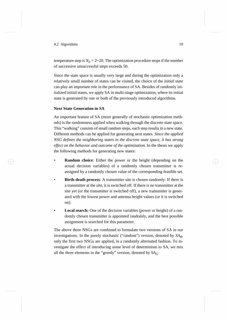
4.2 Algorithms 59
temperature step is N0 = 2~20. The optimization procedure stops if the numberof successive unsuccessful steps exceeds 50.
Since the state space is usually very large and during the optimization only arelatively small number of states can be visited, the choice of the initial statecan play an important role in the performance of SA. Besides of randomly ini-tialized initial states, we apply SA in multi-stage optimization, where its initialstate is generated by one or both of the previously introduced algorithms.
Next State Generation in SA
An important feature of SA (more generally of stochastic optimization meth-ods) is the randomness applied when walking through the discrete state space.This “walking” consists of small random steps, each step results in a new state.Different methods can be applied for generating next states. Since the appliedNSG defines the neighboring states in the discrete state space, it has strongeffect on the behavior and outcome of the optimization. In the thesis we applythe following methods for generating new states:
• Random choice: Either the power or the height (depending on theactual decision variables) of a randomly chosen transmitter is re-assigned by a randomly chosen value of the corresponding feasible set.
• Birth-death process: A transmitter site is chosen randomly. If there isa transmitter at the site, it is switched off. If there is no transmitter at thesite yet (or the transmitter is switched off), a new transmitter is gener-ated with the lowest power and antenna height values (or it is switchedon).
• Local search: One of the decision variables (power or height) of a ran-domly chosen transmitter is appointed randomly, and the best possibleassignment is searched for this parameter.
The above three NSGs are combined to formulate two versions of SA in ourinvestigations. In the purely stochastic (“random”) version, denoted by SAR,only the first two NSGs are applied, in a randomly alternated fashion. To in-vestigate the effect of introducing some level of determinism to SA, we mixall the three elements in the “greedy” version, denoted by SAG.

60 Minimal Cost Coverage Planning for SFN based DAB
4.2.4 Combined multi-stage algorithms
Since there are certain limitations of each of the above algorithm, we investi-gate if more powerful algorithms can be constructed with cascading of thoseelements. We have investigated the performance of the following single- andmulti-stage algorithms:
4.3 Performance Results
We have chosen three planning situations with increasing complexity to dem-onstrate the performance characteristics of the algorithms. Two of these threecases were solved by deterministic total search too, in order to be able to makemore reliable comparisons.
In the objective function we use α = 10 and β = 0.5, moreover the interferencepenalty is not considered (γ = 0). The performance measures used for evaluat-ing the algorithms are: (1) best objective value, (2) worst objective value, (3)
No Description Abbreviation
Single stage algorithms:
0 Deterministic Total Search TS
1 Step-by-Step SS
Two-stage algorithms:
First stage: Second stage:
2 Step-by-Step Non-greedy Local Search SS+LSN
3 Step-by-Step Greedy Local Search SS+LSG
4 Random initialization Non-greedy Local Search R+LSN
5 Random initialization Greedy Local Search R+LSG
6 Random initialization Rand. Simulated Annealing R+SAR
7 Step-by-Step Rand. Simulated Annealing SS+SAR
8 Random initialization Greedy SA R+SAG
Three-stage algorithms:
First stage: Second stage: Third stage:
9 Step-by-step G. Local Search Random SA SS+LSN+SAR
Table 4-1 Investigated algorithms. For detailed description of the buildingcomponents see previous sub-sections.

4.3 Performance Results 61
average objective value, (4) variance and (5) average number of visited states(which is proportional to the number of point-to-point path-loss calculationsas well as to the running time). On each case study the algorithms were exe-cuted a number of times, in order to calculate the performance statistics.Algorithms involving SA usually visit one order of magnitude more states dur-ing a single run than others not involving SA. In order to maintain fairness ofthe comparison, non-SA algorithms were repeated 50 times, while SA-basedalgorithms had only five chances.
Case 1: Small scale general design problem
The first test case is a small scale design problem with state space size: There are seven transmitter locations defined on a circular ser-
vice area with radius 50 km over hilly terrain. The feasible power and antennaheight values are P = 35, 45 [dBW] and H = 50, 100 [m], respectively.The corresponding cost values are CS = 80, 90, ... , 140, CP = 50, 100 andCH = 70, 140. DAB mode I is assumed. Cmax is set to 4900.
Figure 4-3 shows the distribution of the objective function values over the totalstate space of the problem calculated by deterministic total search The statespace is apparently divided into two parts due to the severe penalty for net-works not satisfying the constraint. The figure approves our choice of the
Figure 4-3 Distribution of the objective function values over the totalstate space for case 1
ℑ 7.8 4×10≅
0 0.5 1 1.5 2 2.5 3 3.5 40
500
1000
1500
2000
2500
3000
3500
Value of the objective function
Num
ber
of st
ate
s
Case 1: State space

62 Minimal Cost Coverage Planning for SFN based DAB
objective function. There are a very large number of configurations that satisfythe outage probability constraint, but using unnecessarily high hardware cost.Figure 4-4 and Table 4-2 presents the performance results of the ninealgorithms.
Figure 4-4 Performance results of the algorithms for Case 1
Algorithm
Objective function values(Global optimum: 0.3041)
# ofvisitedstatesMean (σ) Min / Max
1 SS 0.4061 (0.0246) 0.3510 / 0.4653 8.1
2 SS+LSN 0.3791 (0.0218) 0.3245 / 0.4204 40.0
3 SS+LSG 0.3669 (0.0226) 0.3041 / 0.4020 39.0
4 R+LSN 0.3450 (0.0245) 0.3041 / 0.4020 41.6
5 R+LSG 0.3496 (0.0203) 0.3184 / 0.4082 41.6
6 R+SAR 0.3457 (0.0204) 0.3102 / 0.3592 552.2
7 SS+SAR 0.3363 (0.0129) 0.3184 / 0.3510 557.8
8 R+SAG 0.3514 (0.0191) 0.3327 / 0.3776 466.2
9 SS+LSG+SAR 0.3269 (0.0172) 0.3041 / 0.3469 598.8
Table 4-2 Performance results of the algorithms for Case 1
valu
e of
the
obje
ctiv
e fu
nctio
n
opt
mean
min
max
1 2 3 4 5 6 7 8 90.2
0.25
0.3
0.35
0.4
0.45
0.5
Algorithms
Case 1
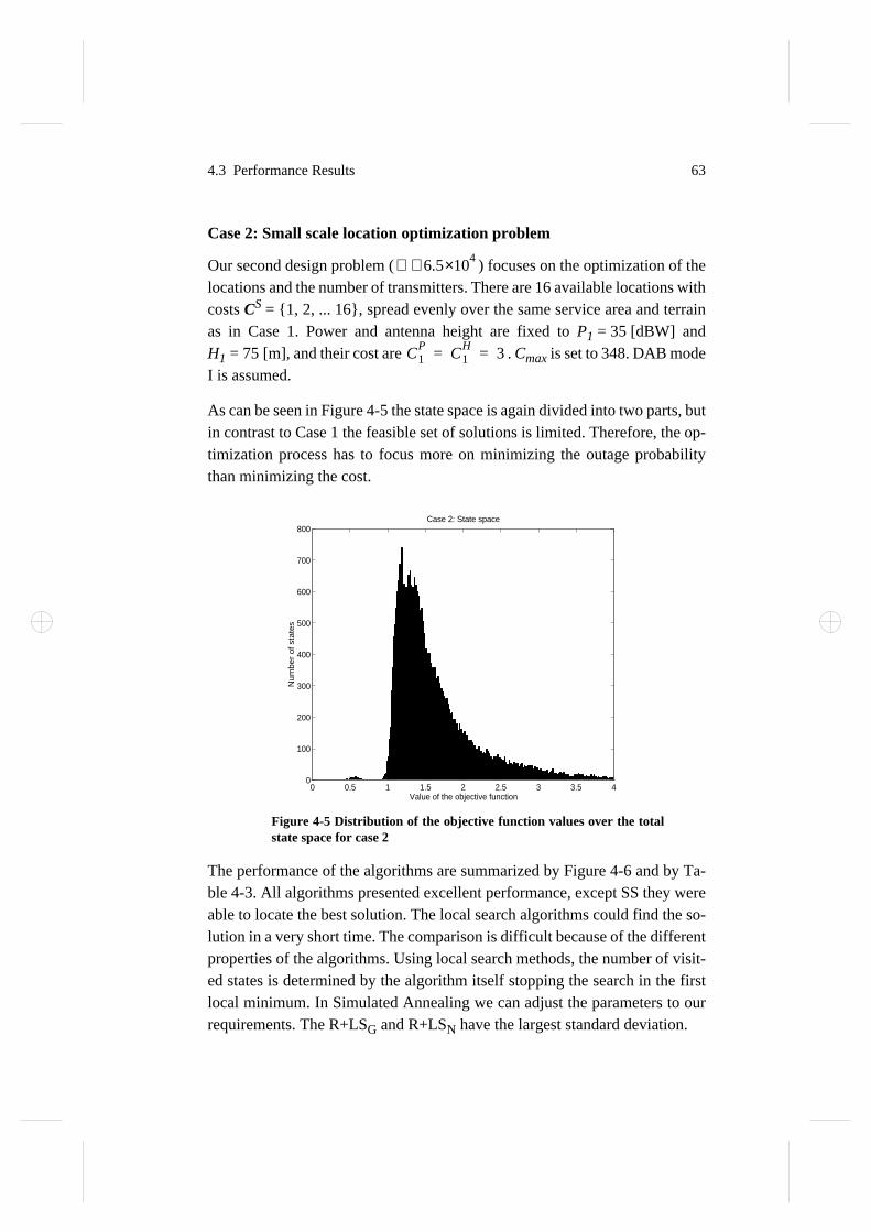
4.3 Performance Results 63
Case 2: Small scale location optimization problem
Our second design problem ( ) focuses on the optimization of thelocations and the number of transmitters. There are 16 available locations withcosts CS = 1, 2, ... 16, spread evenly over the same service area and terrainas in Case 1. Power and antenna height are fixed to P1 = 35 [dBW] andH1 = 75 [m], and their cost are . Cmax is set to 348. DAB modeI is assumed.
As can be seen in Figure 4-5 the state space is again divided into two parts, butin contrast to Case 1 the feasible set of solutions is limited. Therefore, the op-timization process has to focus more on minimizing the outage probabilitythan minimizing the cost.
The performance of the algorithms are summarized by Figure 4-6 and by Ta-ble 4-3. All algorithms presented excellent performance, except SS they wereable to locate the best solution. The local search algorithms could find the so-lution in a very short time. The comparison is difficult because of the differentproperties of the algorithms. Using local search methods, the number of visit-ed states is determined by the algorithm itself stopping the search in the firstlocal minimum. In Simulated Annealing we can adjust the parameters to ourrequirements. The R+LSG and R+LSN have the largest standard deviation.
Figure 4-5 Distribution of the objective function values over the totalstate space for case 2
ℑ 6.5 4×10≅
C1P
C1H 3= =
0 0.5 1 1.5 2 2.5 3 3.5 40
100
200
300
400
500
600
700
800
Value of the objective function
Num
ber
of st
ate
s
Case 2: State space
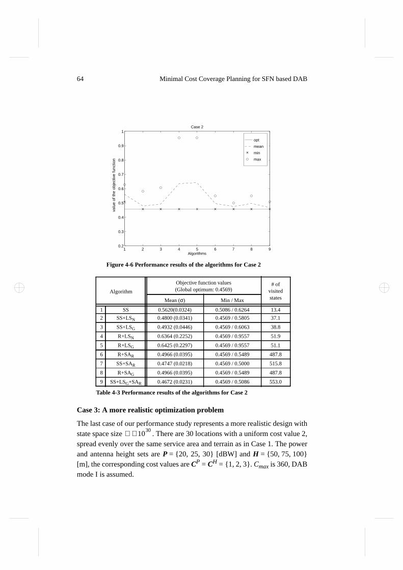
64 Minimal Cost Coverage Planning for SFN based DAB
Case 3: A more realistic optimization problem
The last case of our performance study represents a more realistic design withstate space size . There are 30 locations with a uniform cost value 2,spread evenly over the same service area and terrain as in Case 1. The powerand antenna height sets are P = 20, 25, 30 [dBW] and H = 50, 75, 100[m], the corresponding cost values are CP = CH = 1, 2, 3. Cmax is 360, DABmode I is assumed.
Figure 4-6 Performance results of the algorithms for Case 2
Algorithm
Objective function values(Global optimum: 0.4569)
# ofvisitedstatesMean (σ) Min / Max
1 SS 0.5620(0.0324) 0.5086 / 0.6264 13.4
2 SS+LSN 0.4800 (0.0341) 0.4569 / 0.5805 37.1
3 SS+LSG 0.4932 (0.0446) 0.4569 / 0.6063 38.8
4 R+LSN 0.6364 (0.2252) 0.4569 / 0.9557 51.9
5 R+LSG 0.6425 (0.2297) 0.4569 / 0.9557 51.1
6 R+SAR 0.4966 (0.0395) 0.4569 / 0.5489 487.8
7 SS+SAR 0.4747 (0.0218) 0.4569 / 0.5000 515.8
8 R+SAG 0.4966 (0.0395) 0.4569 / 0.5489 487.8
9 SS+LSG+SAR 0.4672 (0.0231) 0.4569 / 0.5086 553.0
Table 4-3 Performance results of the algorithms for Case 2
valu
e of
the
obje
ctiv
e fu
nctio
n
opt
mean
min
max
1 2 3 4 5 6 7 8 90.2
0.3
0.4
0.5
0.6
0.7
0.8
0.9
1
Algorithms
Case 2
ℑ 1030≅

4.3 Performance Results 65
In this problem Simulated Annealing outstripped the other algorithms, as wecan see in Figure 4-7 and in Table 4-4. The result indicates that in such largescale problems there exist several local minimum solutions, where the appli-cation of Simulated Annealing has a large advantage jumping over severallocality.
Figure 4-7 Performance results of the algorithms for Case 3
Algorithm
Objective function values(Global optimum: unknown)
# ofvisitedstates
Mean (σ) Min / Max
1 SS 0.3876 (0.0240) 0.3361 / 0.4444 76.8
2 SS+LSN 0.3571 (0.0231) 0.3139 / 0.4111 259.7
3 SS+LSG 0.3565 (0.0284) 0.2972 / 0.4111 218.5
4 R+LSN 0.3427 (0.0945) 0.2833 / 0.7898 243.8
5 R+LSG 0.3334 (0.1276) 0.2472 / 0.8384 187.8
6 R+SAR 0.2822 (0.0140) 0.2667 / 0.3028 2821.6
7 SS+SAR 0.2694 (0.0056) 0.2639 / 0.2750 2982.6
8 R+SAG 0.2917 (0.0212) 0.2583 / 0.3111 2194.4
9 SS+LSG+SAR 0.2850 (0.0266) 0.2500 / 0.3167 3000.8
Table 4-4 Performance results of the algorithms for Case 3
valu
e of
the
obje
ctiv
e fu
nctio
n
mean
min
max
1 2 3 4 5 6 7 8 90.2
0.25
0.3
0.35
0.4
0.45
0.5
Algorithms
Case 3

66 Minimal Cost Coverage Planning for SFN based DAB
Conclusions from the three case studies
Based upon the numerical results of the three case studies, a number of generalconclusions can be drawn.
• Three-stage SS+LSR+SAR was consistently the best performingalgorithm.
• Determinism (greediness) involved in the next state generation proce-dure did not improve performance of SA.
• It is hard to say anything about the advantage or drawback to applygreediness in LS, both versions showed quite similar performance.
• In the location optimization case (Case 2) LS had major difficulties.This can be explained by the lack of ability to relocate transmitters.Relocation would require LS to remove a transmitter in one step andcreate another transmitter in a later step, or vice versa. Removal is usu-ally barred by the serious temporary degradation of the coverage, whileimplementation of a new transmitter fails because the unjustifiedincreasement of network cost. This drawback of LS could probably beeliminated (or at least alleviated) with altering the neighbourhood defi-nition, e.g. by introducing state changes that directly relocatetransmitters. Such extensions to LS are recommended for furtherstudies.
• As a consequence of the above, randomly initialized LS was very incon-sistent in Case 2 where the location of transmitters was a major issue.
• However, it is interesting to see that the best results of randomly initial-ized LS are better than of SS based LS. This indicates an interestingfeature of SS, namely that although it consistently finds a relativelygood solution, it is also very consistently far from being near to the bestsolution. Since LS is very much trapped in the neighbourhood of thesolution given by SS, the final solution of the two stages remains "mid-dle-class".
• SS based LS is more reliable and consistent (in terms of variance andworst case solution) than its randomly initialized peer, consequently, itwas more appropriate to use as a feeder method to SA in the three-stagealgorithm than any other methods.

4.3 Performance Results 67
• The capability of SA to skip out from local minima is especially attrac-tive in cost sensitive design cases, e.g. when cost is an important issueand there are a large number of satisfying solutions with wide range ofcost values. In such cases LS sticks to the neighbourhood of the solutionfound by SS (or generated randomly) resulting in solutions that are sat-isfying the constraints, but totally disregarding cost. SA spendsconsiderable efforts in the search to further minimize the total cost.

68 Minimal Cost Coverage Planning for SFN based DAB

69
Chapter 5
Practical SFN Planning
5.1 Cost sensitive network planning
In this subsection, we present the effects of different cost configurations in thesame design problem. The trials is performed in a national planning task. Inthis case, DAB Mode I (Tg=246 µs, Ts=1000 µs) is used. The area is 100 x 100km with max. height difference 300 m. The testpoints are selected on regulargrid with distance of 1 km. There are 30 potential transmitter sites, each rep-resents an available FM transmitter site where the new transmitter can easilybe placed. The interference environment is not considered. The feasible set ofpower values is P = 20, 25, 30, 33, 35 [dBW] and, the feasible set of antennaheight values is H = 50, 100, 150, 200, 250 [m]. Two different cost config-urations are applied during the optimization as defined by Table 5-1 and Table5-2.
For both cost configurations the optimization is performed by algorithmR+SA, 20 times. The resulted network configurations are evaluated by the fre-quency of the transmitters with power and antenna height values of P and H.
P[dBW] 20 25 30 33 35
CP 30 200 700 2100 3150
H [m] 50 100 150 200 250
CH 80 150 900 1650 2100
Table 5-1 Cost configuration with CS = 100
P[dBW] 20 25 30 33 35
CP 30 100 400 700 1050
H [m] 50 100 150 200 250
CH 80 150 300 550 700
Table 5-2 Cost configuration with CS = 500
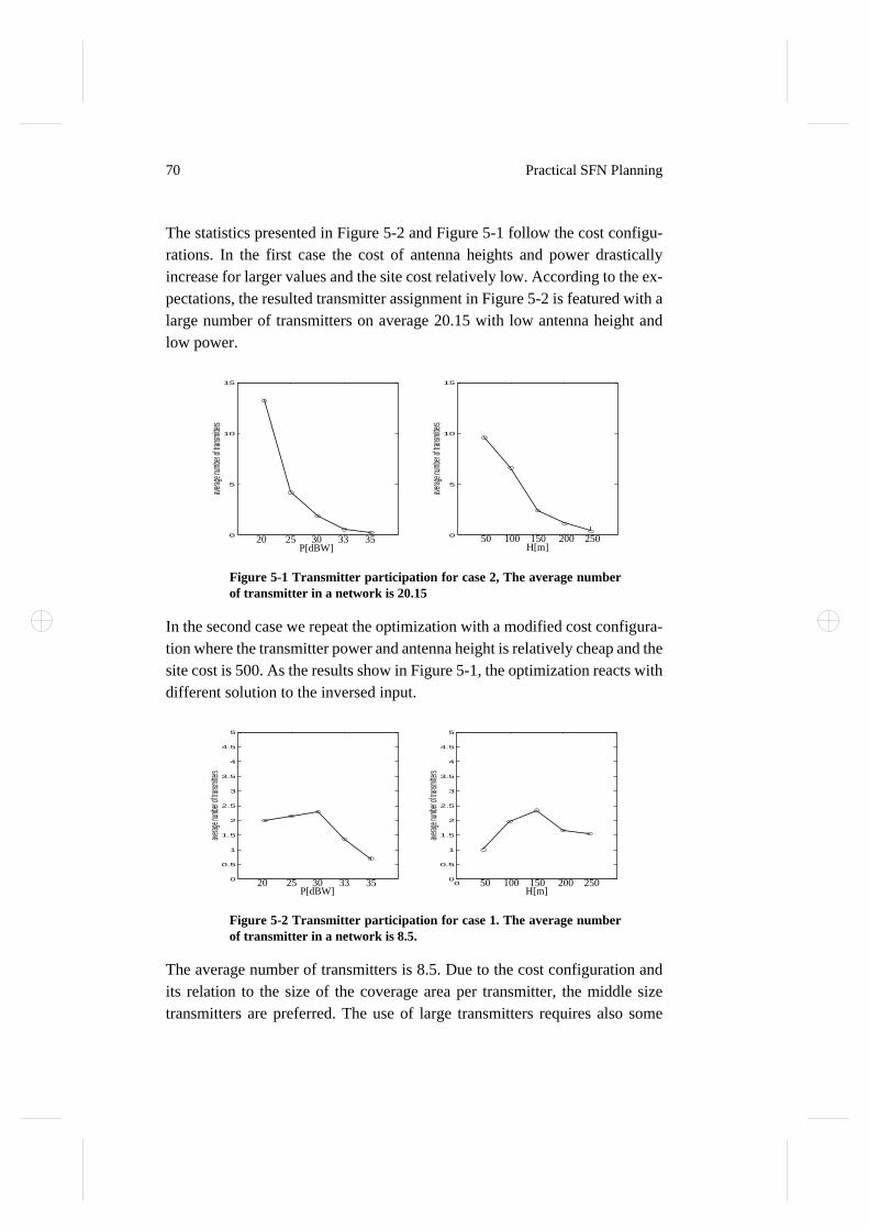
70 Practical SFN Planning
The statistics presented in Figure 5-2 and Figure 5-1 follow the cost configu-rations. In the first case the cost of antenna heights and power drasticallyincrease for larger values and the site cost relatively low. According to the ex-pectations, the resulted transmitter assignment in Figure 5-2 is featured with alarge number of transmitters on average 20.15 with low antenna height andlow power.
In the second case we repeat the optimization with a modified cost configura-tion where the transmitter power and antenna height is relatively cheap and thesite cost is 500. As the results show in Figure 5-1, the optimization reacts withdifferent solution to the inversed input.
The average number of transmitters is 8.5. Due to the cost configuration andits relation to the size of the coverage area per transmitter, the middle sizetransmitters are preferred. The use of large transmitters requires also some
Figure 5-1 Transmitter participation for case 2, The average numberof transmitter in a network is 20.15
Figure 5-2 Transmitter participation for case 1. The average numberof transmitter in a network is 8.5.
0
5
10
15
averag
e num
ber of
transm
itters
0
5
10
15
averag
e num
ber of
transm
itters
20 25 30 33 35P[dBW]
50 100 150 200 250H[m]
0
0.5
1
1.5
2
2.5
3
3.5
4
4.5
5
averag
e num
ber of
transm
itters
00
0.5
1
1.5
2
2.5
3
3.5
4
4.5
5
averag
e num
ber of
transm
itters
20 25 30 33 35P[dBW]
50 100 150 200 250H[m]
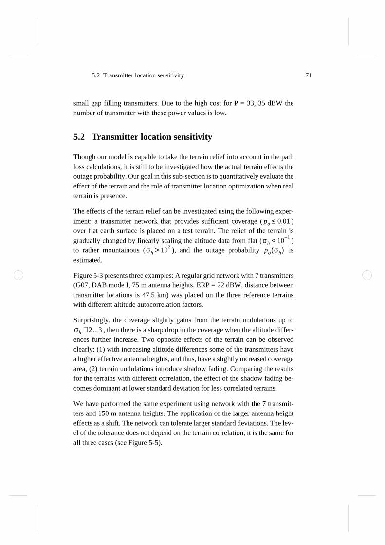
5.2 Transmitter location sensitivity 71
small gap filling transmitters. Due to the high cost for P = 33, 35 dBW thenumber of transmitter with these power values is low.
5.2 Transmitter location sensitivity
Though our model is capable to take the terrain relief into account in the pathloss calculations, it is still to be investigated how the actual terrain effects theoutage probability. Our goal in this sub-section is to quantitatively evaluate theeffect of the terrain and the role of transmitter location optimization when realterrain is presence.
The effects of the terrain relief can be investigated using the following exper-iment: a transmitter network that provides sufficient coverage ( )over flat earth surface is placed on a test terrain. The relief of the terrain isgradually changed by linearly scaling the altitude data from flat ( )to rather mountainous ( ), and the outage probability isestimated.
Figure 5-3 presents three examples: A regular grid network with 7 transmitters(G07, DAB mode I, 75 m antenna heights, ERP = 22 dBW, distance betweentransmitter locations is 47.5 km) was placed on the three reference terrainswith different altitude autocorrelation factors.
Surprisingly, the coverage slightly gains from the terrain undulations up to, then there is a sharp drop in the coverage when the altitude differ-
ences further increase. Two opposite effects of the terrain can be observedclearly: (1) with increasing altitude differences some of the transmitters havea higher effective antenna heights, and thus, have a slightly increased coveragearea, (2) terrain undulations introduce shadow fading. Comparing the resultsfor the terrains with different correlation, the effect of the shadow fading be-comes dominant at lower standard deviation for less correlated terrains.
We have performed the same experiment using network with the 7 transmit-ters and 150 m antenna heights. The application of the larger antenna heighteffects as a shift. The network can tolerate larger standard deviations. The lev-el of the tolerance does not depend on the terrain correlation, it is the same forall three cases (see Figure 5-5).
po 0.01≤
σh 10 1–<σh 102> po σh( )
σh 2...3∼
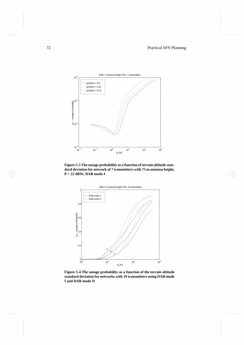
72 Practical SFN Planning
Figure 5-3 The outage probability as a function of terrain altitude stan-dard deviation for network of 7 transmitters with 75 m antenna height,P = 22 dBW, DAB mode-I
Figure 5-4 The outage probability as a function of the terrain altitudestandard deviation for networks with 19 transmitters using DAB modeI and DAB mode II
ρ(10km) = 0.5
ρ(10km) = 0.32
ρ(10km) = 0.15
10−2
10−1
100
101
102
103
10−3
10−2
10−1
100
σh [m]
po −
ou
tag
e p
rob
ab
ility
DAB−I, Antenna height 75m, 7 transmitters
DAB mode−I DAB mode−II
100
101
102
103
0
0.2
0.4
0.6
0.8
1
σh [m]
po −
ou
tag
e p
rob
ab
ility
DAB I−II, Antenna height 75m, 19 transmitters
ab
c
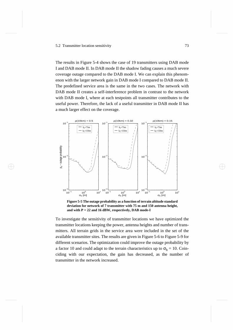
5.2 Transmitter location sensitivity 73
The results in Figure 5-4 shows the case of 19 transmitters using DAB modeI and DAB mode II. In DAB mode II the shadow fading causes a much severecoverage outage compared to the DAB mode I. We can explain this phenom-enon with the larger network gain in DAB mode I compared to DAB mode II.The predefined service area is the same in the two cases. The network withDAB mode II creates a self-interference problem in contrast to the networkwith DAB mode I, where at each testpoints all transmitter contributes to theuseful power. Therefore, the lack of a useful transmitter in DAB mode II hasa much larger effect on the coverage.
To investigate the sensitivity of transmitter locations we have optimized thetransmitter locations keeping the power, antenna heights and number of trans-mitters. All terrain grids in the service area were included in the set of theavailable transmitter sites. The results are given in Figure 5-6 to Figure 5-9 fordifferent scenarios. The optimization could improve the outage probability bya factor 10 and could adapt to the terrain characteristics up to σh = 10. Coin-ciding with our expectation, the gain has decreased, as the number oftransmitter in the network increased.
Figure 5-5 The outage probability as a function of terrain altitude standarddeviation for network of 7 transmitter with 75 m and 150 antenna height,and with P = 22 and 16 dBW, respectively, DAB mode-I
10−1
100
101
10−3
10−2
10−1
σh [m]
p o −
out
age
prob
abilit
y
ρ(10km) = 0.5
10−1
100
101
10−3
10−2
10−1
σh [m]
ρ(10km) = 0.32
10−1
100
101
10−3
10−2
10−1
σh [m]
ρ(10km) = 0.15
-- ht=75m
ht=150m
-- ht=75m
ht=150m
-- ht=75m
ht=150m
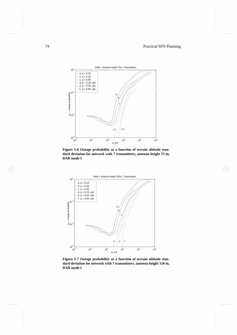
74 Practical SFN Planning
Figure 5-6 Outage probability as a function of terrain altitude stan-dard deviation for network with 7 transmitters, antenna height 75 m,DAB mode I
Figure 5-7 Outage probability as a function of terrain altitude stan-dard deviation for network with 7 transmitters, antenna height 150 m,DAB mode I
10−2
10−1
100
101
102
103
10−3
10−2
10−1
100
σh [m]
po −
ou
tag
e p
rob
ab
ility
DAB−I, Antenna height 75m, 7 transmitters
a
b
c
d e−f
a: ρ = 0.15b: ρ = 0.32c: ρ = 0.50d: ρ = 0.15, opt.e: ρ = 0.32, opt.f: ρ = 0.50, opt.
10−2
10−1
100
101
102
103
10−3
10−2
10−1
100
σh [m]
po −
ou
tag
e p
rob
ab
ility
DAB−I, Antenna height 150m, 7 transmitters
a
b
c
de f
a: ρ = 0.15b: ρ = 0.32c: ρ = 0.50d: ρ = 0.15, opt.e: ρ = 0.32, opt.f: ρ = 0.50, opt.
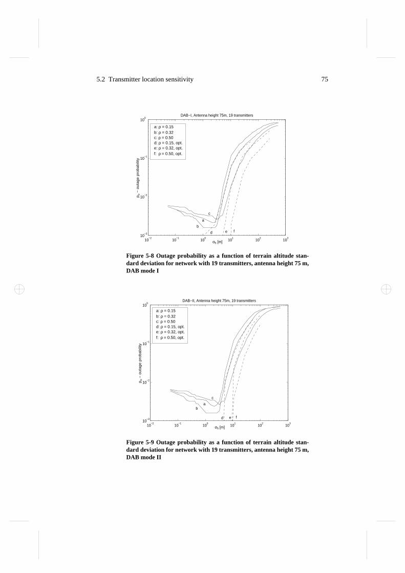
5.2 Transmitter location sensitivity 75
Figure 5-8 Outage probability as a function of terrain altitude stan-dard deviation for network with 19 transmitters, antenna height 75 m,DAB mode I
Figure 5-9 Outage probability as a function of terrain altitude stan-dard deviation for network with 19 transmitters, antenna height 75 m,DAB mode II
10−2
10−1
100
101
102
103
10−3
10−2
10−1
100
σh [m]
po −
ou
tag
e p
rob
ab
ility
DAB−I, Antenna height 75m, 19 transmitters
b
a
c
d e f
a: ρ = 0.15b: ρ = 0.32c: ρ = 0.50d: ρ = 0.15, opt.e: ρ = 0.32, opt.f: ρ = 0.50, opt.
10−2
10−1
100
101
102
103
10−3
10−2
10−1
100
σh [m]
po −
ou
tag
e p
rob
ab
ility
DAB−II, Antenna height 75m, 19 transmitters
ab
c
d e f
a: ρ = 0.15b: ρ = 0.32c: ρ = 0.50d: ρ = 0.15, opt.e: ρ = 0.32, opt.f: ρ = 0.50, opt.
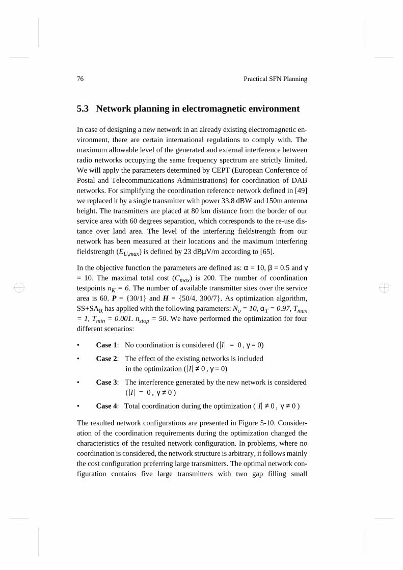
76 Practical SFN Planning
5.3 Network planning in electromagnetic environment
In case of designing a new network in an already existing electromagnetic en-vironment, there are certain international regulations to comply with. Themaximum allowable level of the generated and external interference betweenradio networks occupying the same frequency spectrum are strictly limited.We will apply the parameters determined by CEPT (European Conference ofPostal and Telecommunications Administrations) for coordination of DABnetworks. For simplifying the coordination reference network defined in [49]we replaced it by a single transmitter with power 33.8 dBW and 150m antennaheight. The transmitters are placed at 80 km distance from the border of ourservice area with 60 degrees separation, which corresponds to the re-use dis-tance over land area. The level of the interfering fieldstrength from ournetwork has been measured at their locations and the maximum interferingfieldstrength (EU,max) is defined by 23 dBµV/m according to [65].
In the objective function the parameters are defined as: α = 10, β = 0.5 and γ= 10. The maximal total cost (Cmax) is 200. The number of coordinationtestpoints nK = 6. The number of available transmitter sites over the servicearea is 60. P = 30/1 and H = 50/4, 300/7. As optimization algorithm,SS+SAR has applied with the following parameters: No = 10, αT = 0.97, Tmax
= 1, Tmin = 0.001. nstop = 50. We have performed the optimization for fourdifferent scenarios:
• Case 1: No coordination is considered ( , γ = 0)
• Case 2: The effect of the existing networks is includedin the optimization ( , γ = 0)
• Case 3: The interference generated by the new network is considered( , )
• Case 4: Total coordination during the optimization ( , )
The resulted network configurations are presented in Figure 5-10. Consider-ation of the coordination requirements during the optimization changed thecharacteristics of the resulted network configuration. In problems, where nocoordination is considered, the network structure is arbitrary, it follows mainlythe cost configuration preferring large transmitters. The optimal network con-figuration contains five large transmitters with two gap filling small
I 0=
I 0≠
I 0= γ 0≠
I 0≠ γ 0≠
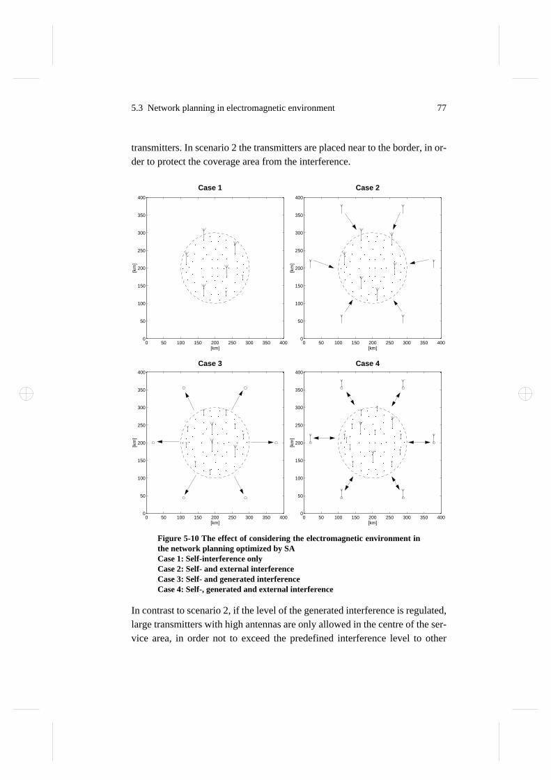
5.3 Network planning in electromagnetic environment 77
transmitters. In scenario 2 the transmitters are placed near to the border, in or-der to protect the coverage area from the interference.
In contrast to scenario 2, if the level of the generated interference is regulated,large transmitters with high antennas are only allowed in the centre of the ser-vice area, in order not to exceed the predefined interference level to other
Figure 5-10 The effect of considering the electromagnetic environment inthe network planning optimized by SACase 1: Self-interference onlyCase 2: Self- and external interferenceCase 3: Self- and generated interferenceCase 4: Self-, generated and external interference
0 50 100 150 200 250 300 350 4000
50
100
150
200
250
300
350
400
[km]
[km
]
0 50 100 150 200 250 300 350 4000
50
100
150
200
250
300
350
400
[km]
[km
]
Case 1 Case 2
Case 3 Case 4
0 50 100 150 200 250 300 350 4000
50
100
150
200
250
300
350
400
[km]
[km
]
0 50 100 150 200 250 300 350 4000
50
100
150
200
250
300
350
400
[km]
[km
]

78 Practical SFN Planning
networks. At the border we can find transmitters only with low antennaheights. Scenario 4 keeps the property of scenario 3, whereas to satisfy thecoverage requirements of own against the increased interference level addi-tional transmitters are required.
In our problem omnidirectional antenna pattern is used for all transmitters.Another solution is suggested in [65], using directional antennas pointed to thecenter of the service area at the border. In this case the coordination can be per-formed in a second phase.
79
Chapter 6
Conclusions
6.1 Discussion
In the thesis we have focused on the cost minimized coverage planning of SFNin existing electromagnetic environment. The coverage planning is formulatedas an optimization problem, where the transmitter parameters as power, anten-na height and location construct the decision variables. The objective functionwas the collective cost of the transmitters in the network. The outage proba-bility and maximum allowable interference level requirements were includedin the objective function as a penalty.
In order to make reliable outage probability estimation by means of sampling(testpoint) techniques, characteristics of the service area and different sam-pling techniques were investigated. The proper testpoint distance was shownto be strongly related to the terrain characteristics, to the applied propagationmodel and to the level of the total outage. The outage areas for noise limitednetworks are located at low altitudes. Whereas, in interference limited case theprobability of outage are also increased for the high altitudes. In case of un-known interference, it is very difficult to determine the expected place of theoutage. Concerning the dependency of the outage on the relative distance fromtransmitters, the majority of the non-covered points are found farther from thetransmitters.
The performance of the sampling methods have been evaluated on a largenumber of networks, in terms of their required sample size to achieve a givenconfidence level. It was shown that systematic sampling came out as the bestin most of the cases. The proper testpoint distance for systematic sampling canbe determined from the correlation status of the outage.

80 Conclusions
An alternative improvement method of the estimation was investigated by us-ing stratified sampling. The stratified sampling method shown relatively poorperformance compared to our expectation. The explanation comes from the bi-nary nature of our sampled variable. Nevertheless, for some specific casessuch as the noise limited case on approx. flat terrain “network-based” sam-pling shown considerable gain over SRS.
We determined the required minimum number of samples to achieve a re-quired confidence as a function of the outage probability. Due to the fact, thatduring the optimization different network configurations with different outagelevels are evaluated, we recommend the application of sequential sampling.
In the optimization of the coverage for SFN, our primary objective function isdefined as the network hardware cost. The constraints are the technical perfor-mance measures such as the required maximum outage probability and themaximum allowable level of caused interference. The problem is reformulatedby including the constraints in the objective function as a penalty.
The investigation of the state space using deterministic total search approvedour decision to include the network hardware cost in the optimization. Thereexist several network configurations that satisfy our technical requirements.Therefore, instead of optimizing further the technical parameters, minimizingthe network cost can give significant cost reduction. Of course, the gain de-pends on the predefined values of the feasible sets of power, antenna heightand transmitter locations. These sets determine the size of the feasible and in-feasible regions of the optimization problem.
Different types of optimization techniques have been investigated and com-pared through case studies. For solving relatively small scale problems allalgorithms performed well, the heuristics and local search algorithm couldfind the solution in very short time. In more complicated problems with largestate space Simulated Annealing outstripped the other algorithms. It showsthat in such large scale problems there exist several local minimum solutionsand efficient optimization requires the ability of escaping from local minima.
In cases when location optimization is a major issue, LS had difficulties,which can be explained by the lack of ability to relocate transmitters. Reloca-tion would require LS to remove a transmitter in one step and create anothertransmitter in a later step, or vice versa. Removal is usually barred by the se-
6.1 Discussion 81
rious temporary degradation of the coverage, while implementation of a newtransmitter fails because the unjustified increasement of network cost. Thisdrawback of LS could probably be eliminated (or at least alleviated) with al-tering the neighbourhood definition, e.g. by introducing state changes thatdirectly relocate transmitters. Such extensions to LS are recommended for fur-ther studies.
The capability of SA to skip out from local minima is especially attractive incost sensitive design cases, e.g. when cost is an important issue and there area large number of satisfying solutions with wide range of cost values. In suchcases LS sticks to the neighbourhood of the solution found by SS (or generatedrandomly) resulting in solutions that are satisfying the constraints, but totallydisregarding cost. SA spends considerable efforts in the search to further min-imize the total cost.
We have investigated the sensitivity of transmitter locations for given test net-work configurations in presence of the terrain with different correlation anddifferent standard deviation of altitude. Comparing with coverage on flat ter-rain, the coverage slightly gains from the terrain undulations up to σh = 2-3 mbecause of the increased effective antenna height of some of the transmitters.Coverage drops drastically when the altitude differences further increase, dueto the increasing shadow fading effect. For less correlated terrain this effectappears at smaller altitude differences. For DAB mode II the effect is muchsevere than in case of DAB I. We can explain this phenomenon with the largernetwork gain in DAB mode I compared to mode II.
To investigate the gain of optimization we have optimized the transmitter lo-cations keeping the power, antenna heights and number of transmitters fixed.The optimization could improve the outage probability by a factor of 10 andcould adapt to the terrain characteristics up to σh ~ 10m. Coinciding with ourexpectations, the gain has decreased, as the number of transmitter in the net-work increased.
Consideration of the coordination requirements during the optimizationchanged the characteristics of the resulted network configuration. In problems,where no coordination was considered, the network structure was quite regularand perfectly adapted to the cost configuration. In case of coordination, thetransmitters at the border of the service area were assigned by low antenna

82 Conclusions
heights, in order not to exceed the predefined interference level. Coordinatednetworks required slightly higher cost.
6.2 Future work
One of the objectives is to continue the research on digital broadcasting net-work design with the following alternative subjects:
• Use of heuristic optimization technique based on network analysis andapplication of improved stochastic planning tools including continuousvariables (e.g. for power and antenna height)
• Network design included frequency and delay planning
• Local and wide area coverage optimization in the same time (frequencyand network sharing) i.e: how to combine several applications to reducethe total cost. Using the same infrastructure to different applicationswith different requirements.
• Reducing the self-interference for larger local SFNs: Transmitter delaytuning, i.e. select the transmission instant such the areas that where ear-lier not covered properly gets a better lower self-interferenceenvironment.
• Investigation of the Power-Sum methods used for mobile cellular net-work planning for broadcasting application and comparing with theCCIR methods

83
References
Digital Terrain Database:
[1] Maguire, D., J., Goodchild, M., F., Rhind, D., W., “Geographical Infor-mation Systems: Principles and Applications”, Longman Scientific &Technical with John Wiley & Sons, New York, ISBN 0-582-05661-6,1991
[2] Perez Fontan, F., Hernando, J., M., “Selection of Digital Terrain DataBase Parameters for Radiocommunication System Planning Applica-tions”, IEEE Trans. on Broadcasting, Vol. 39, No. 3, September 1993
Propagation model:
[3] CCIR Rec. 370-5, “VHF and UHF Propagation Curves for the Fre-quency Range from 30 MHz to 1000 MHz”, 1990
[4] Longley, A., G., Rice, P., L., “Prediction of Tropospheric Radio Trans-mission Loss over Irregular Terrain”, Inst. for Telecomm. Sci., Boulder,Colorado, ESSA Tech. Report ERL-79-ITS-67
[5] Bullington, K., “Radio Propagation at Frequencies Above 30 Megacy-cles", Proceedings of the I.R.E. - Waves and Electrons Section, October1947.
[6] Deygout, J., “Multiple Knife-Edge Diffraction of Microwaves”, IEEETrans. on Antennas and Propagation, Vol. Ap-14, No. 4, July 1966.
[7] Giovaneli, C., L., “An Analysis of Simplified Solution for MultipleKnife-Edge Diffraction”, IEEE Trans. on Antennas and Propagation,Vol. Ap-32, No. 3, March 1984.
[8] Blomquist, Å., Ladell, L., “Prediction and Calculation of TransmissionLoss in Different Types of Terrain”, FOA 3 Rapport, C 3792-E2, June1974.
[9] Ladell, L., “Transmission Loss Predictions in Wooded Terrain”, NordicRadio Symposium, Conference Proceedings pp41-50, Saltsjbaden,Sweden, 15-17 April, 1986

84
[10] Lee, W., C., Y., “Mobile Communications Engineering”, McGraw-HillBook Company, ISBN 0-07-037039-7, Chapter 4: Path Loss over HillyTerrain and General Methods of Prediction
[11] Grosskopf, R., “Comparison of Different Methods for the Prediction ofthe Field Strength in the VHF Range”, IEEE Trans. on Antennas andPropagation, Vol. Ap-35, No. 7, July 1987
[12] Grosskopf, R., “Comparison of Field Strength Prediction Methods inthe UHF Range”, Proc. of the Sixth Int. Conf. Antennas and Propaga-tion, ICAP 89, IEE No. 301, part 2, pp 350-354
[13] Perez Fontan, F., Hernando, J., M., “Comparison of Irregular TerrainPropagation Models for Use in Digital Terrain Data Based Radiocom-munication System Planning Tools”, IEEE Trans. on Broadcasting,Vol. 41, No. 2, June 1995.
[14] Asp, B., Holm, P., “Application of GTD to Radio Path Loss Predic-tions”, Proc. NRS-95 Nordic Radio Symposium, ISBN 91-630-3415-8
[15] Lebherz, M., Wiesbeck, W., Blasberg, H.-J., Krank, W., “Calculation ofbroadcast coverage based on a digital terrain model”, Proc. of the SixthInt. Conf. Antennas and Propagation, ICAP 89, IEE No. 301, part 2, pp355-359
[16] Lebherz, M., Wiesbeck, W., Krank, W., “A versatile wave propagationmodel for the VHF/UHF range considering three-dimensional terrain”,IEEE Trans. on Antennas and Propagation, Vol.Ap-40, No.10, pp1121-1131, 1992
[17] Kurner, T., Cichon, D.-J., Wiesbeck, W., “Concepts and Results for 3DDigital Terrain-Based Wave Propagation Model”, IEEE JSAC, Vol.11,No.7, September 1993
Coverage probability and multiple interference calculation:
[18] CCIR Rep. 945-2, “Methods for the Assessment of Multiple Interfer-ence”, 1990.
[19] O’Leary, T., Rutkowski, J., “Combining multiple interfering fieldstrengths: the simplified multiplication method and its physical andmathematical basis”, Telecommunication Journal Vol. 49 -XII/1982
[20] Brugger, R., “Comparative analysis of standard methods for the combi-nation of multiple interfering fieldstrengths”, GT RT/DIG 063, GT R4

85
383, Munich, December 1991
[21] Brugger, R., “Treatment of minimum fieldstrength in coverage calcula-tions for digital services”, GT R1/DIG 205, January 1994
[22] Schwartz, S. C., Yeh, Y. S., “On the Distribution Function andMoments of Power Sums With Log-Normal Components”, The BellSystem Technical Journal, Vol. 61, No. 7, September 1982
Statistics and Sampling theory:
[23] Papoulis, A., “Probability, Random Variables and Stochastic Pro-cesses”, Third Edition, McGraw-Hill International Editions, ISBN 0-07-100870-5, 1991
[24] Blom, G., “Probability and Statistics, Theory and Applications”,Springer-Verlag, ISBN 0-387-96852-0, 1989
[25] Ripley, B.-D., “Spatial Statistics”, Wiley Series in Probability andMathematical Statistics, John Wiley & Sons, ISBN 0-471-08367-4,1981
[26] Cochran, W., G., “Sampling Techniques”, Wiley Publications in Statis-tics, John Wiley & Sons, 1953
[27] Thompson, S., K., Seber, G., A., “Adaptive Sampling”, Wiley series inProbability and Statistics, John Wiley & Sons, ISBN 0-471-55871-0,1996
[28] Quellmalz, A., Krank, W., Wiesbeck, W., “Transmitter Network Mod-elling for Efficient Frequency Assignment Applications”, SeventhInternational Conference on antennas and Propagation, University ofYork, UK, 15-16 April 1991.
[29] Sega, W., Marszalek, A., “EM environment analysis of broadcastingnetwork in VHF/UHF namd based on test point concept”, Proceedingsof the Symposium on EMC, Wroclaw, Poland, pp. 678-680, 1992.
Optimization techniques:
[30] Nemhauser, G., L., Rinnooy Kan, A.H.G., Todd, M.J., “Optimization”,Handbooks in Operations Research and Management Science, NorthHolland, Elsevier Science Publishers B.V., 1989, ISBN 0-444-87284-1
[31] Luenberger, D. G., “Linear and nonlinear programming”, AddisonWesley, 1989.
86
[32] Parker, R., G., Rardin, R., L., “Discrete Optimization”, AcademicPress, Inc. 1988, ISBN 0-12-545075-3
[33] Christofides, N., Mingozzi, A., Toth, P., Sandi, C., “CombinatorialOptimization”, John Wiley & Sons, 1979
[34] Kirkpatrick, S., Gelatt, C.D., Vecchi, M.P., “Optimization by SimulatedAnnealing”, Science, Vol. 220, No. 4598, May 1983.
[35] Laarhoven, P., J., M., Aarts, E., H., L., “Simulated Annealing: Theoryand Applications”, D. Reidel Publishing Company 1987, ISBN 90-277-2513-6
[36] Hajek, B., “Cooling schedules for optimal annealing”, Mathematics ofHale, K., W., “Frequency Assignment: Theory and Applications”, Pro-ceedings of the IEEE, Vol. 68, No. 12, December 1980.
[37] Hale, K., W., “Frequency Assignment: Theory and Applications”, Pro-ceedings of the IEEE, Vol. 68, No. 12, December 1980.
[38] Cesky, T., “Computerized VHF/FM frequency assignments using aMonte-Carlo method”, EBU Review-Technical, No. 231, October1988.
[39] Quellmalz, A., Knälmann, A., Krank, W., “Simulated Annealing as atool for transmitter network planning” (German), RundfunktechnischeMitteilungen, Vol. 37, No. 1, pp18-31, 1993
[40] Ligeti, A., “Verification, Analysis and Improvement of StochasticAlgorithms for Channel Assignment” (German), Ms. C. thesis, Techni-cal University of Karlsruhe, Germany, 1992.
[41] Ligeti, A., Szekeres, B., Zsuffa, Z., “Assignment of Broadcasting Fre-quencies by Utilizing Stochastic Optimization and Digital TerrainDatabase”, Proceedings of the Symposium on EMC, Wroclaw, Poland,pp. 488-492, 1994
[42] M. Dugue Anton, D. Kunz, B. Ruber, “Channel Assignment for Cellu-lar Radio Using Simulated Annealing”, IEEE Trans. on VehicularTechnology, Vol. 42, No. 1, February 1993.
[43] Mathar, R., Mattfeldt, J., “Channel Assignment in Cellular Radio Net-works”, IEEE Trans. on Vehicular Technology, Vol. 42, No. 4,November 1993.

87
Digital Audio Broadcasting:
[44] Alard, M., Lassalle, R., “Principles of modulation and channel codingfor digital broadcasting for mobile receivers”, EBU Technical Review,No. 224, August 1987
[45] CCETT: “Analysis of Interfering Effects in a Single Frequency Net-work”, GT V4/RSM 93, September, 1989
[46] CCETT: “Description of the COFDM system”, [3] is included, GT V4/RSM 148, May, 1990
[47] Rault, J.C., Pillet, D., Castelain, D., “Time Synchronisation of the DABreceiver in a SFN network”, CCETT, Ref: SRL/DHN/089/94/JCR,April 1994
[48] ---, “Technical Bases for the CEPT T-DAB Planning Conference”,Draft, GT R1/DIG 170 Rev. 2, Copenhagen Dec 93/Kingswood Jan 94
[49] Hunt, K. J., Cesky, T., Jeacock, T., Mägele, M., O’Leary, T., Petke, G.,“The CEPT T-DAB Planning Meeting, Wiesbaden, July 1995”, EBUTechnical Review, Spring 1996
[50] European Telecommunication Standard Institute, “Radio broadcast sys-tems; Digital Audio Broadcasting (DAB) to mobile, portable and fixedreceivers”, Draft prevision ETS 300 401, March 1994.
[51] Plenge, G., “DAB - A new sound broadcasting system Status of thedevelopment - Routes to its introduction”, EBU Technical Review, No.246, April 1991.
[52] Lau, A., Williams, W.F., “Service planning for terrestrial Digital AudioBroadcasting”, EBU Technical Review, Summer 1992.
[53] Lee, M., B., R., “Planning Methods for National Single Frequency Net-work for DAB”, IEE, 8th International Conference on Antennas andPropagation, Vol. 2, London 1993
[54] Prosch, T., A., “The Digital Audio Broadcast Single Frequency Net-work Project in Southwest Germany”, IEEE Trans. Broadcasting, Vol.40, No. 4, December 1994.
[55] Brugger, R., “DAB Coverage of Interfering Single Frequency Net-works”, GT R1/DIG 167, June 1993
[56] Lau, A., “Minimum wanted fieldstrength for T-DAB planning”, GT R1/DIG 221

88
[57] Bell, C.P., Williams, W.F., “DAB: Minimum Separation Distances forSingle Frequency Networks”, BBC Contribution, GT R1/DIG 181,October 1993
[58] Lau, A., Pausch, M., Wutschner, W., “First results of field tests with theDAB single frequency network in Bavaria”, EBU Technical Review,Autumn 1994
[59] Rebhan, R., Zander, J., “On the Outage Probability in Single FrequencyNetworks for Digital Broadcasting”, IEEE Trans. Broadcasting, Vol.39, No. 4, December 1993.
[60] Malmgren, G., “On Local/Regional Single Frequency Networks”, Nor-dic Radio Symposium, Conference Proceedings pp. 189-194, April1995.
[61] Malmgren, G., “On the Outage Probability in Local/Regional SingleFrequency Broadcasting Networks”, Kluwer, Wireless Personal Com-munications, Vol. 2, Issue 2/2, 1996
[62] Μalmgren, G., “Network Planning of Single Frequency BroadcastingNetworks”, Technical Licentiate, TRITA-S3-RST-9602, ISSN 1400-9137, ISRN KTH/RST/R-96/02-SE, KTH Dept. of Signals, Sensors andSystems, 1994
[63] Μalmgren, G., “Single Frequency Broadcasting Networks”, PhD The-sis, TRITA-S3-RST-970x, ISSN 1400-9137, ISRN KTH/RST/R-97/0x-SE, KTH Dept. of Signals, Sensors and Systems, 1997
[64] Beutler, R., “Optimization of Digital Single Frequency Networks”, Fre-quenz, Vol. 49, No. 11-12, November-December 1995
[65] Kuchen, F., Becker, T. C., Wiesbeck, W., “Optimizing the CoverageArea of Single Frequency Networks”, International Broadcasting Con-vention, London, U.K., 1996
[66] Ligeti, A., “On Coverage Optimization in Single Frequency Networkusing Simulated Annealing”, Dept. Report TRITA-IT R 95-06, ISRNKTH/IT/R-95/06-SE, KTH Dept. of Teleinformatics, Sweden, 1995
[67] Ligeti, A., “On Coverage Optimization in Single Frequency Networkfor Digital Broadcasting using Simulated Annealing”, Nordic RadioSymposium, Conference Proceedings pp. 67-72, April 1995.

89
Appendix A
Simulated Annealing
The Simulated Annealing developed by Kirkpatrick, Gelatt, Vecchi in 1982[34] is a application of Metropolis-algorithm with a monotone decreasing con-trol parameter so-called “temperature” for solving combinatorial optimizationproblems.
The Metropolis-algorithm was applied at first for investigation of physicalproperties of systems in thermodynamic balance. The principle of the algo-rithm: The algorithm creates an order of states of material. Two consecutivestates are different from each other only in a small particle (e.g. in a molecule).Let Ei be the energy of the state that is reached after the i-th algorithm step. Attime i we select a new state by means of some next state generation procedure.This new state is accepted to become the i+1st state reached by the algorithmwith probability pacc. The acceptance probability is given by the followingexpression:
(A-1)
By applying Metropolis-algorithm with a decreasing temperature the Simulat-ed Annealing (SA) models the crystallization process of the material. Theprocess results in a crystal structure with minimal energy.
Application of the process for mathematical optimization problem can be es-tablished via the following equivalence:
• A state of the parameters-space of the optimization problem corre-sponds a state of the material.
• The value of objective function in a state corresponds to the energy ofthe material in this state.
pacc
1 Ei 1+ Ei<
exp Ei 1+ Ei–( ) T⁄–( ) Ei 1+ Ei≥
=
90 Appendix A: Simulated Annealing
• A control parameter T, which is equivalent with the physical tempera-ture of material, has also been introduced and after the analogy it iscalled as “Temperature”.
The analogy between the cooling a fluid and optimization may fail in one im-portant respect. In ideal fluids all the atoms are alike and the optimal state is aregular crystal, while a typical optimization problem will contain many dis-trict, noninterchangeable elements, so a regular solution is unlikely. It is nowbelieved, that the state space of the coverage optimization has many nearlyequal local optima rather than one outstanding global one. Furthermore, dueto the asymmetry no equivalent state transitions exist during the optimization.
Basic structure of the algorithm
The steps of SA are shown in Figure A-1. The optimization starts from a ran-domly chosen initial state at the given maximal temperature (Tmax). Theenergy of the state E(S) is calculated. From this state will be establish a newstate (S’) with energy E(S’) by applying a suitable next state generation mech-anism. Depending on the energy difference (dE), if the new energy is lowerthan the previous, the new state will be accepted, else the new state is accepteddepending on the acceptance probability. In the exterior cycle the temperaturestairwise decreases until a given minimal temperature (Tmin) is reached, and inevery temperature step the next state generation, energy calculation and stateacceptance is performed several times.
The important feature of algorithm is that a worse state can be accepted, thusthe algorithm can jump out from the local minimum. At the beginning of thecooling process (at high temperature), a worse state can be accepted by thesame probability than a better one, then with decreasing temperature the prob-ability of acceptance of states with higher energy will decrease, and at the endof the cooling process only the states with lower energy will be accepted. Theacceptance probability depending on the temperature and energy difference isshown in Figure A-1.
The disadvantage of acceptance of worse states is, that we can lose the best so-lution during the process. Avoiding this problem it is worth continuouslysaving the actual best solution.

91
Figure A-1 Flow-chart of Simulated Annealing
Energy-difference
START
Generate initial state (S)
Calculate the energy of S
Set initial temperatureT(0) = Tmax
Generate a new state (S’)
Calculate E(S’)
S = S’
T(i+1) = αΤ * T(i)
yes
no
dE = E(S’) - E(S)
for j = 1 ... N0
for i = 1 ... NT
dE < 0
p > x RV (0..1)
probability of acceptance S’p = exp((-dE) / T(i))yes
no
END

92 Appendix A: Simulated Annealing
The definition of energy (object) function of the optimization requires carefulconsiderations. We have to express our requirements with one value for everystate. This energy is calculated in every steps, that requires a quick calculationfor it. The next state generation determines the neighborhood of every state(set of states), that the algorithm can reach from the actual state with one step.Assuming exponential cooling, the parameters of cooling process are the max-imal initial temperature (Tmax), the minimal (final) temperature (Tmin) and theannealing factor (αΤ). These three parameters determine the cooling processtogether. After the theory, these parameters can be set in the following way:
• At the beginning on Tmax the states with the highest energy and the low-est energy should be accepted with same probability. It means, that theacceptance probability must be high (90-99 percentage) both for highestand smallest energy differences (max dE, min dE).
• At the end on Tmin the algorithm has to allow the acceptance states withonly smaller energy
• The transition has to be slow enough, we have to apply a annealing fac-tor 0.96-0.99.
A suitable cooling process and acceptance probability are presented in FigureA-3 and Figure A-1. N0 is number of state changes at a single temperature step.The number of temperature steps NT can be calculated as follows:
(A-2)
Figure A-2 Acceptance probability as a function of dE
1 2 3 dE
Pacc = exp(-dE / T)
T decreased(Cooling)
-1
T min T max αTNT⋅=

93
Figure A-3 Temperature during the cooling process(Tmax = 10, Tmin = 0.001, αΤ = 0.97)
Figure A-4 Acceptance probability during the cooling processfor max dE (0.5) and min dE (0.01)
0 50 100 150 200 250 3000
1
2
3
4
5
6
7
8
9
10
Temperature steps
Tem
pera
ture
dur
ing
the
cool
ing
proc
ess
0 50 100 150 200 250 3000
0.1
0.2
0.3
0.4
0.5
0.6
0.7
0.8
0.9
1
Temperature steps
Acce
ptan
ce p
roba
bility
max dE
min dE

94 Appendix A: Simulated Annealing


Radio Communication Systems Lab.Dept. of Signals, Sensors and SystemsRoyal Institute of TechnologyS-100 44 STOCKHOLMSWEDEN
TRITA—S3—RST—9702ISSN 1400—9137
ISRN KTH/RST/R-- 97/02 --SE

Agn
es L
iget
iC
over
age
Opt
imiz
atio
n in
Dig
ital
Aud
io B
road
cast
ing
Net
wor
ksK
TH
199
7