cover new impa ceris 2010 - Boston Collegefm · Cerulli G., Working Paper Cnr-Ceris, N° 05/2014 ....

WorkingPaperWorkingPaper

ISTITUTO DI RICERCASULL’IMPRESA E LO SVILUPPO

ISSN (print): 1591-0709ISSN (on line): 2036-8216

Co

nsi

gli

o N

azio

na

le d

ell

e R

ice

rch

e

cover new impa ceris 2010 26-01-2010 7:36 Pagina 1

e.viarisio

Casella di testo

l Working paper Cnr-Ceris, N.05/2014 l CTREATREG: STATA MODULE FOR ESTIMATING DOSE-RESPONSE MODELS UNDER EXOGENOUS AND ENDOGENOUS TREATMENT l Giovanni Cerulli

Cerulli G., Working Paper Cnr-Ceris, N° 05/2014

Copyright © 2014 by Cnr-Ceris All rights reserved. Parts of this paper may be reproduced with the permission of the author(s) and quoting the source.

Tutti i diritti riservati. Parti di quest’articolo possono essere riprodotte previa autorizzazione citando la fonte.

WORKING PAPER CNR - CERIS

RIVISTA SOGGETTA A REFERAGGIO INTERNO ED ESTERNO

ANNO 16, N° 5 – 2014 Autorizzazione del Tribunale di Torino

N. 2681 del 28 marzo 1977

ISSN (print): 1591-0709 ISSN (on line): 2036-8216

DIRETTORE RESPONSABILE

Secondo Rolfo

DIREZIONE E REDAZIONE Cnr-Ceris Via Real Collegio, 30 10024 Moncalieri (Torino), Italy Tel. +39 011 6824.911 Fax +39 011 6824.966 [email protected] www.ceris.cnr.it

COMITATO SCIENTIFICO

Secondo Rolfo

Giuseppe Calabrese

Elena Ragazzi

Maurizio Rocchi

Giampaolo Vitali

Roberto Zoboli

SEDE DI ROMA Via dei Taurini, 19 00185 Roma, Italy Tel. +39 06 49937810 Fax +39 06 49937884

SEDE DI MILANO Via Bassini, 15 20121 Milano, Italy tel. +39 02 23699501 Fax +39 02 23699530

SEGRETERIA DI REDAZIONE Enrico Viarisio [email protected]

DISTRIBUZIONE On line: www.ceris.cnr.it/index.php?option=com_content&task=section&id=4&Itemid=64

FOTOCOMPOSIZIONE E IMPAGINAZIONE In proprio

Finito di stampare nel mese di Aprile 2014


CTREATREG: Stata module for estimating

dose-response models under exogenous and endogenous treatment

Giovanni Cerulli

CNR - National Research Council of Italy CERIS - Institute for Economic Research on Firm and Growth

Via dei Taurini 19, 00185 Roma, ITALY

Mail: [email protected]

Tel.: 06-49937867

ABSTRACT: This paper presents ctreatreg, a Stata module for estimating a dose-response function when: (i) treatment is continuous, (ii) individuals may react heterogeneously to observable confounders, and (iii) selection-into-treatment may be endogenous. Two estimation procedures are implemented: OLS under Conditional Mean Independence, and Instrumental-Variables (IV) under selection endogeneity. A Monte Carlo experiment to test the reliability of the proposed command is finally set out.

Keywords: Stata commands; treatment effects, dose-response function, continuous treatment, Monte Carlo, R&D support

JEL Codes: C21, C87, D04


4

CONTENTS

1. Introduction .............................................................................................................................. 5

2. The model ................................................................................................................................ 6

3. The regression approach .......................................................................................................... 7

3.1 Estimation under Unconfoundedness .......................................................................... 8

3.2 Estimation under treatment endogeneity ..................................................................... 9

3.3 Estimation of comparative dose-response functions ................................................. 11

4. The Stata routine ctreatreg .............................................................................................. 11

5. An instructional application ................................................................................................... 13

6. A Monte Carlo experiment for testing ctreatreg’s reliability......................................... 19

7. Conclusion ............................................................................................................................. 21

References ................................................................................................................................... 22


5

1. INTRODUCTION

his paper presents a Stata routine,

ctreatreg, for estimating a

dose-response function through a

regression approach when: (i) treatment is

continuous, (ii) individuals may react

heterogeneously to observable confounders,

and (iii) selection-into-treatment may be

potentially endogenous. In this context, the

dose-response function is equal to the

“Average Treatment Effect, given the level

of treatment t” (i.e. ATE(t)). But also other

causal parameters of interest, such as the

unconditional Average Treatment Effect

(ATE), the Average Treatment Effect on

Treated (ATET), the Average Treatment

Effect on Non-Treated (ATENT) are

estimated by ctreatreg, along with

those effects conditional on the vector (x; t),

where x is a vector of pre-determined

variables.

Such a routine seems of worth, as in

many socio-economic and epidemiological

contexts, interventions take the form of a

continuous exposure to a certain type of

treatment. Indeed, from a program

evaluation perspective, what is relevant in

many settings is not only the binary

treatment status, but also the level of

exposure (or “dose”) provided by a public

agency.

This is also in tune with the language of

epidemiology, where dose-response

functions are usually estimated in order to

check patients’ resilience to different levels

of drug administration (Robertson et al.,

1994; Royston and Sauerbrei, 2008).

To fix ideas, consider a policy program

where the treatment is assigned not

randomly (i.e., according to some

“structural” rule), and where – after setting

who is treated and who is not – the program

provides a different “level” or “exposure”

to treatment ranging from 0 (no treatment)

to 100 (maximum treatment level). Two

groups of units are thus formed: (i)

untreated, whose level of treatment (or

dose) is zero, and (ii) treated, whose level

of treatment is greater than zero.

We are interested in estimating the causal

effect of the treatment variable t on an

outcome y within the observed sample, by

assuming that treated and untreated units

may respond differently both to specific

observable confounders (that we collect in a

vector x), and to the “intensity” of the

treatment t. We wish to estimate a dose-

response function of y on t, either when the

treatment is assumed to be exogenous (i.e.,

selection-into-treatment depends only on

observable-to-analyst factors) or

endogenous (i.e., selection-into-treatment

depends both on observable and

unobservable-to-analyst factors).

Compared with similar models - and in

particular the one proposed by Hirano and

Imbens (2004) implemented in Stata by Bia

and Mattei (2008)1 - this model does not

need a full normality assumption, and it is

well-suited when many individuals have a

zero-level of treatment (“spike” or no-nil

probability mass at zero as in Royston et al.

(2010)). Additionally, it may account for

treatment “endogeneity” by exploiting an

1 See also Bia, Flores and Mattei (2011) generalizing

the Hirano-Imbens (2004) model by allowing for a

nonparametric estimation of the Dose-Response

Function. Furthermore, see Guardabascio and

Ventura (2013) for an extension of the Hirano-

Imbens model allowing for various non-normal

distributions of the continuous-treatment variable.

T


6

Instrumental-Variables (IV) estimation in a

continuous treatment context.

The reliability of the model and of its

Stata implementation via ctreatreg is

then checked by a Monte Carlo experiment,

proving that the model and the routine lead

to expected theoretical results.

The routine provides also an interesting

graphical representation of results by

optionally plotting both the conditional

effects’ distribution and the dose-response

function along with its confidence intervals.

The paper is organized as follows: section

2 and 3 present the model, its assumptions

and formulas, as well as the related

estimation techniques (section 3); section 4

presents and explains the use of the Stata

routine ctreatreg; then, the paper goes

on by showing, in section 5, an application

of ctreatreg on real data; section 6 sets

out the results from a related Monte Carlo

experiment to test the routine’s reliability;

section 7, finally, concludes the paper. At

the end of the paper, Table1A reports

ctreatreg’s help-file.

2. THE MODEL

We set out with some notation. Consider

two different and exclusive outcomes: one

referring to a unit i when she is treated, y1i;

and one referring to the same unit when she

is untreated, y0i.

Define wi as the treatment indicator,

taking value 1 for treated and 0 for

untreated units, and xi = (x1i, x2i, x3i, ... , xMi)

as a row vector of M exogenous and

observable characteristics (confounders) for

unit i = 1, ... , N. Let N be the number of

units involved in the experiment, N1 be the

number of treated units, and N0 the number

of untreated units with N = N1 + N0.

Define two distinct functions, g1(xi) and

g0(xi), as the unit i’s responses to the vector

of confounding variables xi when the unit is

treated and untreated respectively. Assume

µ1 and µ0 to be two scalars, and e1 and e0

two random variables having zero

unconditional mean and constant variance.

Finally, define ti – taking values within the

continuous range [0;100] – as the

continuous-treatment indicator, and h(ti) as

a general derivable function of ti.

In what follows, in order to simplify

notation, we’ll get rid of the subscript i

when defining population quantities and

relations.

Given previous notation, we assume a

specific population generating process for

the two exclusive potential outcomes2:

1 1 1 1

0 0 0 0

1: ( ) ( )

0 : ( )

w y g h t e

w y g e

µµ

= = + + + = = + +

x

x

(1)

where the h(t) function is different from

zero only in the treated status. Given this,

we can also define the causal parameters of

interests.

Indeed, by defining the treatment effect as

the difference TE = (y1 – y0), We define the

causal parameters of interests, as the

population Average Treatment Effects

(ATEs) conditional on x and t, that is:

2 Such a model is the representation of a treatment

random coefficient regression as showed by

Wooldridge (1997; 2003). See also Wooldridge

(2010, Ch. 18). For the sake of simplicity, as we refer

to the population model, here we avoid to write the

subscript i referring to each single unit i’s

relationships.


7

1 0

1 0

1 0

ATE( ; ) E( | , )

ATET( ; 0) E( | , 0)

ATENT( ; 0) E( | , 0)

t y y t

t y y t

t y y t

= −> = − >

= = − =

x x

x x

x x

(2)

where ATE indicates the overall average

treatment effect, ATET the average

treatment effect on treated, and ATENT the

one on untreated units. By the law of

iterated expectation (LIE), we know that the

population unconditional ATEs are

obtained as:

( ; )

( ; 0)

( ; 0)

ATE = E ATE( ; )

ATET = E ATE( ; 0)

ATENT = E ATE( ; 0)

t

t

t

t

t

t

>

=

>

=

x

x

x

x

x

x

(3)

where Ez(·) identifies the mean operator

taken over the support of a generic vector of

variables z. By assuming a linear-in-

parameters parametric form for

0( )g = 0x xδ and 1 1( )g =x xδ the

Average Treatment Effect (ATE)

conditional on x and t becomes:

(4)

where µ=(µ1-µ0) and δ=(δ1-δ0) and the

unconditional Average Treatment Effect

(ATE) related to model (1) is equal to:

where p(·) is a probability, and 0th > is the

average of the response function taken

over t > 0. Since, by LIE, we have that

ATE = p(w=1)·ATET + p(w=0)·ATENT,

we obtain from the previous formula that:

where the dose-response function is given

by averaging ATE(x, t) over x:

(6)

that is a function of the treatment intensity

t. The estimation of equation (6) under

different identification hypothesises is the

main purpose of next sections.

3. THE REGRESSION APPROACH

In this section we consider the conditions

for a consistent estimation of the causal

parameters defined in (2) and (3) and thus

of the dose-response function in (6).

What it is firstly needed, however, is a

consistent estimation of the parameters of

the potential outcomes in (1) – we call here

“basic” parameters – as both ATEs and the

dose-response function are functions of

these parameters.

Under previous definitions and

assumptions, and in particular the form of

the potential outcomes in model (1), to be

substituted into Rubin’s potential outcome

equation 0 1 0( )i i i iy y w y y= + − , the

following Baseline random-coefficient

regression can be obtained (Wooldridge,

1997; 2003):

ATE( , , ) [ ( )] (1 ) [ ]t w w h t wµ µ= ⋅ + + + − ⋅ +x xδ δ

ATE( , , ) [ ( )] (1 ) [ ]t w w h t wµ µ= ⋅ + + + − ⋅ +δ xδ

0 0 0ATE = ( 1) ( ) ( 0) ( )t t tp w h p wµ µ> > == ⋅ + + + = ⋅ +x δ δ

0 0 0ATE = ( 1) ( ) ( 0) ( )t t tp w h p wµ µ> > == ⋅ + + + = ⋅ +δ x δ

0 0 0

0 0

0

ATE ( 1)( ) ( 0)( )

ATET

ATENT

µ µµ

µ

> > =

> >

=

= = + + + = +

= + + = +

t t t

t t

t

p w h p w

h

x δ x δ

x δ

x δ

0ATET ( ( ) ) if 0ATE( )

ATENT if 0th t h t

tt

> + − >=

=


8

(7)

where

0 1 0( )i i i i ie w e eη = + ⋅ − .

The equation sets out in (12), provides the

baseline regression for estimating the basic

parameters (µ0, µ1, δ0, δ1, ATE) and then all

the remaining ATEs.

Both a semi-parametric or a parametric

approach can be employed as soon as a

parametric or a non-parametric form of the

function h(t) is assumed.

In both cases, however, in order to get a

consistent estimation of basic parameters,

we need some additional hypotheses. We

start by assuming first Unconfoundedness

or Conditional Mean Independence (CMI),

showing that it is sufficient to provide

parameters’ consistent estimation.

Then we remove this hypothesis and

introduce other identifying assumptions.

3.1 Estimation under Unconfoundedness

Unconfoundedness states that, conditional

on the knowledge of the true exogenous

confounders x, the condition for

randomization are restored, and causal

parameters become identifiable.

Given the set of random variables

y1i, y1i, wi , xi as defined above,

Unconfoundedness (or CMI) implies that:

E(yij | wi , xi) = E(yij | xi) with j = 0,1

CMI is a sufficient condition for

identifying ATEs and the dose-response

function in this context.

Indeed, this assumption entails that, given

the observable variables collected in x, both

w and t are exogenous in equation (7), so

that we can write the regression line of the

response y simply as:

(8)

and Ordinary Least Squares (OLS) can be

used to retrieve consistent estimation of all

parameters.

Once a consistent estimation of the

parameters in (8) is obtained, we can

estimate ATE directly from this regression,

and ATET, ATENT and the dose-response

function by plugging the estimated basic

parameters into formula (5) and (6).

This is possible because these parameters

are functions of consistent estimates, and

thus consistent themselves.

Observe that standard errors for ATET

and ATENT can be correctly obtained via

bootstrapping (see Wooldridge, 2010, pp.

911-919).

To complete the identification of ATEs

and the dose-response function, we finally

assume a parametric form for h(t):

2 3( )i i i ih t at bt ct= + +

(9)

where a, b, and c are parameters to be

estimated in regression (8).

0 ATE ( ) ( ( ) )i i i i i i i iy w w w h t hµ η= + ⋅ + + ⋅ − + ⋅ − +0x δ x x δ

ATE ( ) ( ( ) )i i i i i i i iy w w w h t hµ η= + ⋅ + + ⋅ − + ⋅ − +δ δ

0E( | , , ) ATE ( ) ( ( ) )i i i i i i i i i iy w t w w w h t hµ= + ⋅ + + ⋅ − + ⋅ −0x x δ δ

E( | , , ) ATE ( ) ( ( ) )i i i i i i i i i iy w t w w w h t h= + ⋅ + + ⋅ − + ⋅ −δ x x δ


9

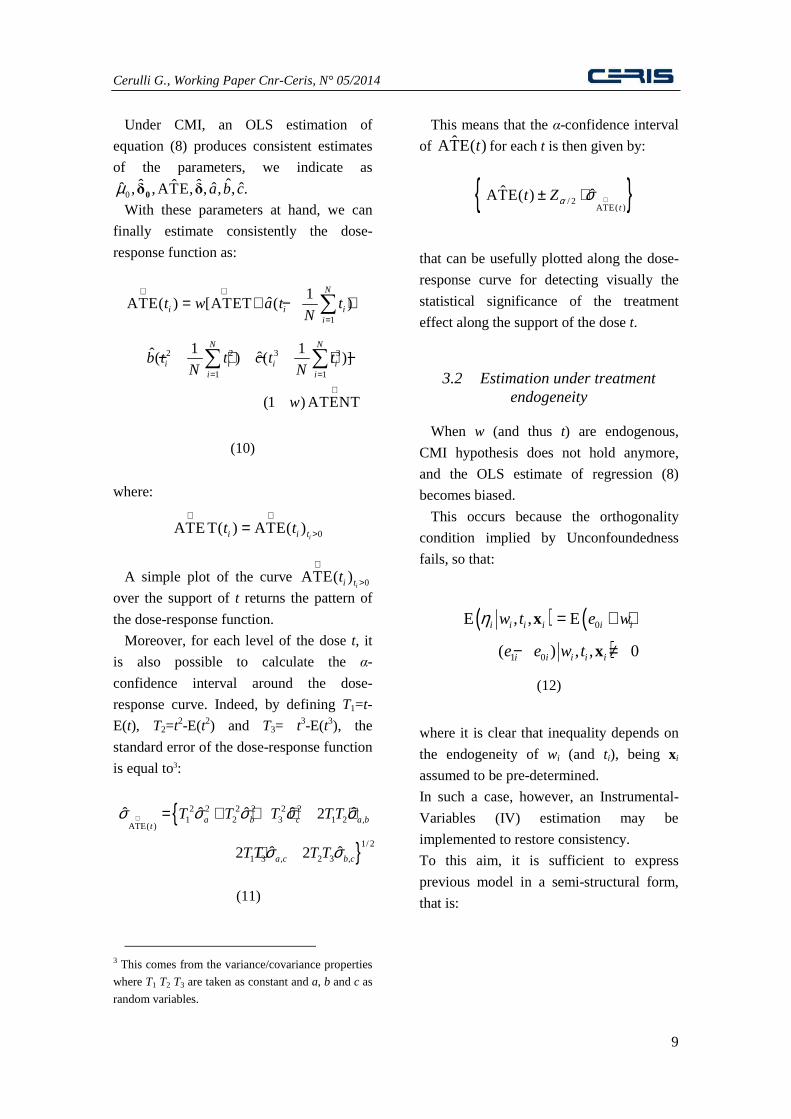
Under CMI, an OLS estimation of

equation (8) produces consistent estimates

of the parameters, we indicate as

0ˆˆ ˆˆˆ ˆ ˆ, ,ATE, , , , .a b cµ 0δ δ

With these parameters at hand, we can

finally estimate consistently the dose-

response function as:

(10)

where:

0ATE T( ) ATE( )ii i tt t

∧ ∧

>=

A simple plot of the curve 0ATE( )∧

>ii ttover the support of t returns the pattern of

the dose-response function.

Moreover, for each level of the dose t, it

is also possible to calculate the α-

confidence interval around the dose-

response curve. Indeed, by defining T1=t-

E(t), T2=t2-E(t2) and T3= t3-E(t3), the

standard error of the dose-response function

is equal to3:

(11)

3 This comes from the variance/covariance properties

where T1 T2 T3 are taken as constant and a, b and c as

random variables.

This means that the α-confidence interval

of ÂTE( )t for each t is then given by:

/ 2ATE( )

ˆ ˆ ATE( )t

t Zα σ ∧± ⋅

that can be usefully plotted along the dose-

response curve for detecting visually the

statistical significance of the treatment

effect along the support of the dose t.

3.2 Estimation under treatment endogeneity

When w (and thus t) are endogenous,

CMI hypothesis does not hold anymore,

and the OLS estimate of regression (8)

becomes biased.

This occurs because the orthogonality

condition implied by Unconfoundedness

fails, so that:

(12)

where it is clear that inequality depends on

the endogeneity of wi (and ti), being xi

assumed to be pre-determined.

In such a case, however, an Instrumental-

Variables (IV) estimation may be

implemented to restore consistency.

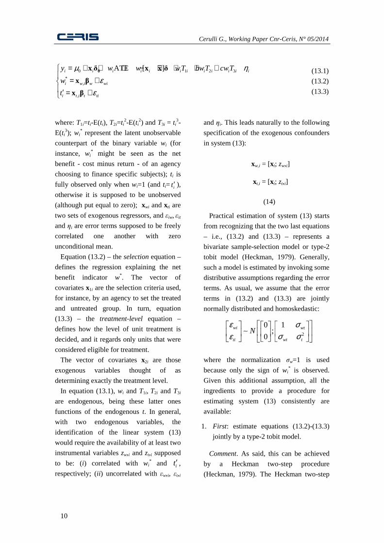
To this aim, it is sufficient to express

previous model in a semi-structural form,

that is:

1 1 1

1 1 1ˆ ÂTE( ) [ATET ( ) ( ) ( )] (1 ) ATENT

N N N

i i i i i i ii i i

t w a t t b t t c t t wN N N

∧ ∧ ∧

= = =

= + − + − + − + −∑ ∑ ∑

2 2 3 3

1 1 1

1 1 1ˆˆ ÂTE( ) [ATET ( ) ( ) ( )] (1 ) ATENTN N N

i i i i i i ii i i

t w a t t b t t c t t wN N N

∧ ∧ ∧

= = =

= + − + − + − + −∑ ∑ ∑

ATE( ) [ATET ( ) ( ) ( )] (1 ) ATENTt w a t t b t t c t t w∧ ∧ ∧

= + − + − + − + −

2 2 2 2 2 21 2 3 1 2 , 1 3 , 2 3 ,

ATE( )ˆ ˆ ˆ ˆ ˆ ˆ ˆ2 2 2a b c a b a c b c

tT T T TT TT T Tσ σ σ σ σ σ σ∧ = + + + + +

1/ 2

1 2 3 1 2 , 1 3 , 2 3 ,ˆ ˆ ˆ ˆ ˆ ˆ ˆ2 2 2a b c a b a c b cT T T TT TT T Tσ σ σ σ σ σ σ= + + + + +

( ) ( 0 1 0E , , E ( ) , , 0i i i i i i i i i i iw t e w e e w tη = + ⋅ − ≠x x

)0 1 0E , , E ( ) , , 0i i i i i i i i i i iw t e w e e w t= + ⋅ − ≠x x


10

0 1 2 3

*,

,

ATE [ ]

i i i i i i i i i i i i

i w i w wi

i t i t ti

y w w wT bwT cwT

w

t

µ ηε

ε

= + + + − + + + +

= +′ = +

0x δ x x δ

x β

x β

(13.1)

(13.2)

(13.3)

where: T1i=ti-E(ti), T2i=ti2-E(ti

2) and T3i = ti3-

E(ti3); wi

* represent the latent unobservable

counterpart of the binary variable wi (for

instance, wi* might be seen as the net

benefit - cost minus return - of an agency

choosing to finance specific subjects); ti is

fully observed only when wi=1 (and ti= it ′ ),

otherwise it is supposed to be unobserved

(although put equal to zero); xwi and xti are

two sets of exogenous regressors, and εiw, εit

and ηi are error terms supposed to be freely

correlated one another with zero

unconditional mean.

Equation (13.2) – the selection equation –

defines the regression explaining the net

benefit indicator w*. The vector of

covariates x1i are the selection criteria used,

for instance, by an agency to set the treated

and untreated group. In turn, equation

(13.3) – the treatment-level equation –

defines how the level of unit treatment is

decided, and it regards only units that were

considered eligible for treatment.

The vector of covariates x2i are those

exogenous variables thought of as

determining exactly the treatment level.

In equation (13.1), wi and T1i, T2i and T3i

are endogenous, being these latter ones

functions of the endogenous t. In general,

with two endogenous variables, the

identification of the linear system (13)

would require the availability of at least two

instrumental variables zw,i and zt,i supposed

to be: (i) correlated with wi* and it′ ,

respectively; (ii ) uncorrelated with εw,i, εt,i

and ηi. This leads naturally to the following

specification of the exogenous confounders

in system (13):

xw,i = [xi; zw,i]

xt,i = [xi; zt,i]

(14)

Practical estimation of system (13) starts

from recognizing that the two last equations

– i.e., (13.2) and (13.3) – represents a

bivariate sample-selection model or type-2

tobit model (Heckman, 1979). Generally,

such a model is estimated by invoking some

distributive assumptions regarding the error

terms. As usual, we assume that the error

terms in (13.2) and (13.3) are jointly

normally distributed and homoskedastic:

2

10;

0wi wt

wt tti

Nε σ

σ σε

∼

where the normalization σw=1 is used

because only the sign of wi* is observed.

Given this additional assumption, all the

ingredients to provide a procedure for

estimating system (13) consistently are

available:

1. First: estimate equations (13.2)-(13.3)

jointly by a type-2 tobit model.

Comment. As said, this can be achieved

by a Heckman two-step procedure

(Heckman, 1979). The Heckman two-step


11

( 1 2 3ˆ ˆ ˆˆ ˆ ˆ ˆ ˆ, , [ ], , ,i wi wi i wi i wi i wi ip p p T p T p T−x x x )

procedure performs a probit of wi on x1i in

the first step using only the N1 selected

observations, and an OLS regression of it ′

on x2i, augmented by the Mills’ ratio

obtained from the probit in the second step,

using all the N observations as predictions

are made also for the censored data.

However, because of the errors’ joint

normality, a maximum-likelihood (ML)

estimation can be also employed; ML leads

to more efficient estimates of βw and βt.

2. Second: compute the predicted values

of wi (i.e. ˆwip ) and ti (i.e. it ) from

the previous type-2 tobit estimation,

and then perform a two-stage

least squares (2SLS) for equation

(13.1) using as instruments

the following exogenous variables

Comment. This 2SLS approach provides

consistent estimation of the basic

coefficients 0, , ATE, , , , a b cµ 0δ δ

(Wooldridge, 2010, pp. 937-951)4.

3. Third: once previous procedure

estimates consistently the basic

parameters in system (13), the causal

parameters of interest - ATEs and the

dose-response function - can be

consistently estimated by the same plug-

in approach used for the OLS case.

4 Observe that instruments used in the 2SLS are based

on the orthogonal projection of wi and ti on the vector

space generated by all the exogenous variables of

system (13).

3.3 Estimation of comparative dose-response functions

Besides the dose-response function and

the other causal parameters of interest as

defined above, the previous model allows

also for calculating the average comparative

response at different level of treatment (as

in Hirano and Imbens, 2004). This quantity

takes this formula:

ATE( , ) E[ ( ) ( )]∆ = + ∆ −t y t y t (15)

Equation (15) identifies the average

treatment effect between two states (or

levels of treatment): t and t + ∆ . Given a

level of ∆ = ∆ , we can get a particular

ATE( , )t ∆ that can be seen as the

“treatment function at ∆” .

4. THE STATA ROUTINE

CTREATREG

The Stata routine ctreatreg estimates

previous dose-response function both under

CMI and under treatment endogeneity5.

The complete Stata help-file of the

routine showing the syntax along with the

options as set out in Table A1, at the end of

this paper.

Here, we just report the syntax and a

comment on the main options.

5 For a Stata implementation when the treatment is

binary see Cerulli (2012).


12

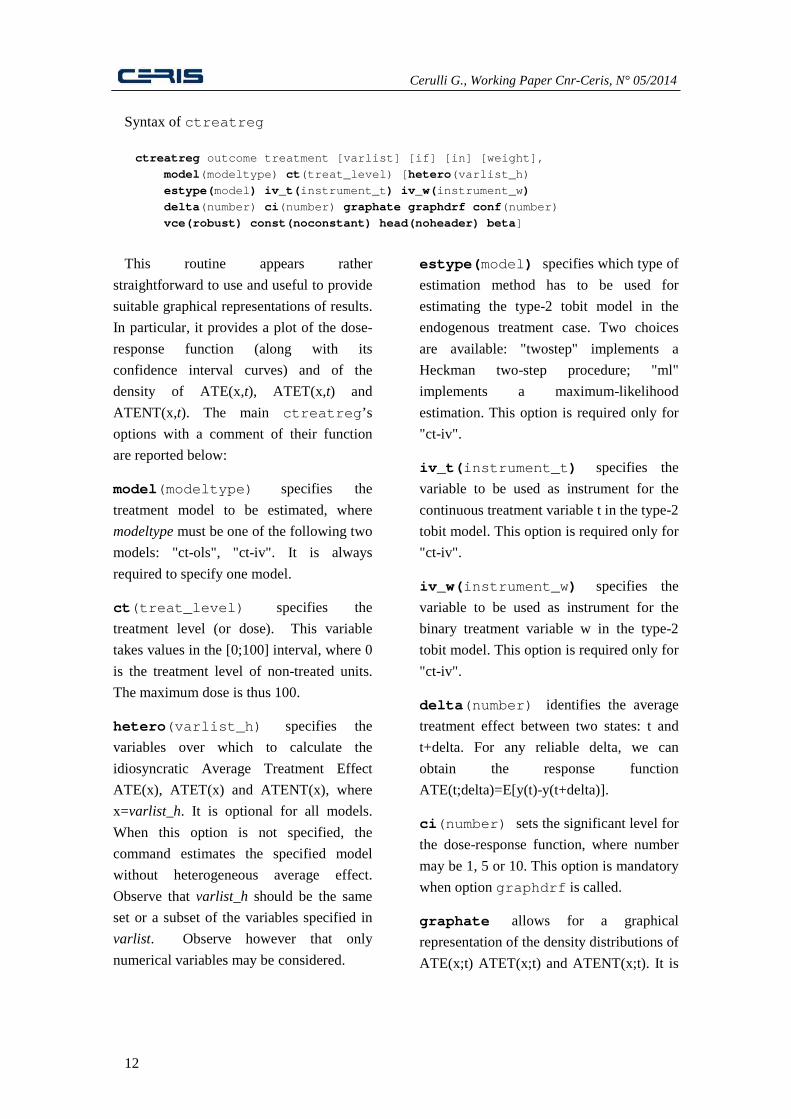
Syntax of ctreatreg ctreatreg outcome treatment [varlist] [if] [in] [weight],

model(modeltype) ct(treat_level) [hetero(varlist_h)

estype(model) iv_t(instrument_t) iv_w(instrument_w)

delta(number) ci(number) graphate graphdrf conf(number)

vce(robust) const(noconstant) head(noheader) beta]

This routine appears rather

straightforward to use and useful to provide

suitable graphical representations of results.

In particular, it provides a plot of the dose-

response function (along with its

confidence interval curves) and of the

density of ATE(x,t), ATET(x,t) and

ATENT(x,t). The main ctreatreg’s

options with a comment of their function

are reported below:

model(modeltype) specifies the

treatment model to be estimated, where

modeltype must be one of the following two

models: "ct-ols", "ct-iv". It is always

required to specify one model.

ct(treat_level) specifies the

treatment level (or dose). This variable

takes values in the [0;100] interval, where 0

is the treatment level of non-treated units.

The maximum dose is thus 100.

hetero(varlist_h) specifies the

variables over which to calculate the

idiosyncratic Average Treatment Effect

ATE(x), ATET(x) and ATENT(x), where

x=varlist_h. It is optional for all models.

When this option is not specified, the

command estimates the specified model

without heterogeneous average effect.

Observe that varlist_h should be the same

set or a subset of the variables specified in

varlist. Observe however that only

numerical variables may be considered.

estype(model) specifies which type of

estimation method has to be used for

estimating the type-2 tobit model in the

endogenous treatment case. Two choices

are available: "twostep" implements a

Heckman two-step procedure; "ml"

implements a maximum-likelihood

estimation. This option is required only for

"ct-iv".

iv_t(instrument_t) specifies the

variable to be used as instrument for the

continuous treatment variable t in the type-2

tobit model. This option is required only for

"ct-iv".

iv_w(instrument_w) specifies the

variable to be used as instrument for the

binary treatment variable w in the type-2

tobit model. This option is required only for

"ct-iv".

delta(number) identifies the average

treatment effect between two states: t and

t+delta. For any reliable delta, we can

obtain the response function

ATE(t;delta)=E[y(t)-y(t+delta)].

ci(number) sets the significant level for

the dose-response function, where number

may be 1, 5 or 10. This option is mandatory

when option graphdrf is called.

graphate allows for a graphical

representation of the density distributions of

ATE(x;t) ATET(x;t) and ATENT(x;t). It is


13

optional for all models and gives an

outcome only if variables into hetero()

are specified.

graphdrf allows for a graphical

representation of the Dose Response

Function (DRF) and of its derivative. By

default, it plots also the 95% confidence

interval of the DRF over the dose levels.

Finally, ctreatreg generates some

useful variables for post-estimation analysis

and returns the estimated treatment effects

into scalars so to get, for instance,

bootstrapped standard errors for ATET and

ATENT that do not have a standard

analytical form (see Table A1).

5. AN INSTRUCTIONAL

APPLICATION

To see how to use ctreatreg in

practice, we consider the Stata 13 example-

dataset “nlsw88.dta” collecting data from

the National Longitudinal Survey of Young

Women of 1988, containing information on

women’s labor conditions such as wages,

educational level, race, marital status, etc..

As an example, we aim at studying the

impact of the variable “tenure” (job tenure)

on “wage” (wages in dollars per hour)

conditional on a series of other covariates

(i.e., observable confounders) referring to

each single woman.

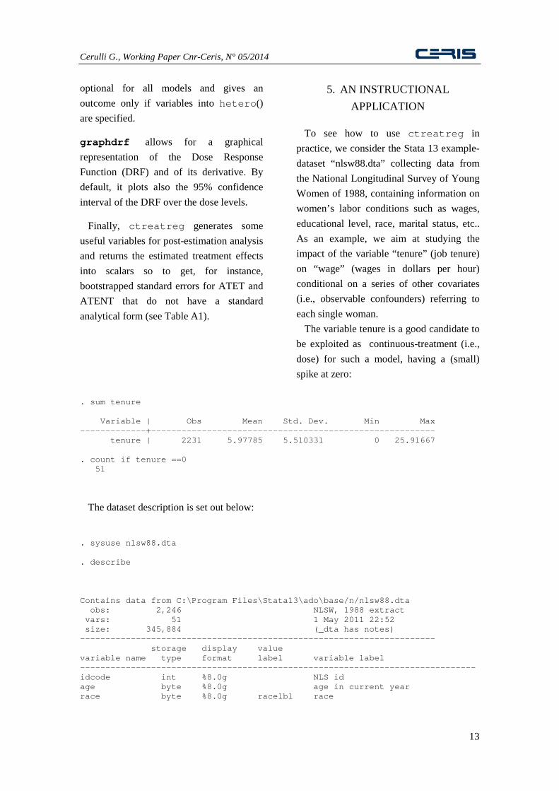
The variable tenure is a good candidate to

be exploited as continuous-treatment (i.e.,

dose) for such a model, having a (small)

spike at zero: . sum tenure Variable | Obs Mean Std. Dev. Min Max -------------+-------------------------------------------------------- tenure | 2231 5.97785 5.510331 0 25.91667 . count if tenure ==0 51

The dataset description is set out below:

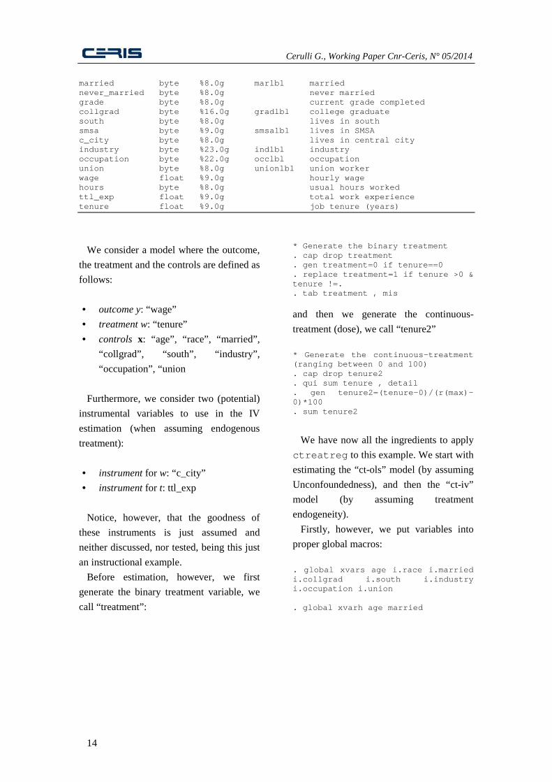
. sysuse nlsw88.dta . describe Contains data from C:\Program Files\Stata13\ado\base/n/nlsw88.dta obs: 2,246 NLSW, 1988 extract vars: 51 1 May 2011 22:52 size: 345,884 (_dta has notes) ---------------------------------------------------------------------- storage display value variable name type format label variable label ------------------------------------------------------------------------------ idcode int %8.0g NLS id age byte %8.0g age in current year race byte %8.0g racelbl race


14

married byte %8.0g marlbl married never_married byte %8.0g never married grade byte %8.0g current grade completed collgrad byte %16.0g gradlbl college graduate south byte %8.0g lives in south smsa byte %9.0g smsalbl lives in SMSA c_city byte %8.0g lives in central city industry byte %23.0g indlbl industry occupation byte %22.0g occlbl occupation union byte %8.0g unionlbl union worker wage float %9.0g hourly wage hours byte %8.0g usual hours worked ttl_exp float %9.0g total work experience tenure float %9.0g job tenure (years)

We consider a model where the outcome,

the treatment and the controls are defined as

follows:

• outcome y: “wage”

• treatment w: “tenure”

• controls x: “age”, “race”, “married”,

“collgrad”, “south”, “industry”,

“occupation”, “union

Furthermore, we consider two (potential)

instrumental variables to use in the IV

estimation (when assuming endogenous

treatment):

• instrument for w: “c_city”

• instrument for t: ttl_exp

Notice, however, that the goodness of

these instruments is just assumed and

neither discussed, nor tested, being this just

an instructional example.

Before estimation, however, we first

generate the binary treatment variable, we

call “treatment”:

* Generate the binary treatment . cap drop treatment . gen treatment=0 if tenure==0 . replace treatment=1 if tenure >0 & tenure !=. . tab treatment , mis

and then we generate the continuous-

treatment (dose), we call “tenure2”

* Generate the continuous-treatment (ranging between 0 and 100) . cap drop tenure2 . qui sum tenure , detail . gen tenure2=(tenure-0)/(r(max)-0)*100 . sum tenure2

We have now all the ingredients to apply

ctreatreg to this example. We start with

estimating the “ct-ols” model (by assuming

Unconfoundedness), and then the “ct-iv”

model (by assuming treatment

endogeneity).

Firstly, however, we put variables into

proper global macros:

. global xvars age i.race i.married i.collgrad i.south i.industry i.occupation i.union . global xvarh age married


15

1. Applying ctreatreg using "ct-ols" (Unconfoundedness):

. xi: ctreatreg wage treatment $xvars , graphrf ///

delta(10) hetero($xvarh) model(ct-ols) ct(tenure2) ci(1)

Source | SS df MS Number of obs = 1851

-------------+------------------------------ F( 36, 1814) = 31.98

Model | 12500.2091 36 347.228032 Prob > F = 0.0000

Residual | 19693.1797 1814 10.8562181 R-squared = 0.3883

-------------+------------------------------ Adj R-squared = 0.3761

Total | 32193.3889 1850 17.4018318 Root MSE = 3.2949

--------------------------------------------------------------------------------

wage | Coef. Std. Err. t P>|t| [95% Conf. Interval]

---------------+----------------------------------------------------------------

treatment | -.9830216 .5226014 -1.88 0.060 -2.007985 .0419421

age | .2534269 .1523452 1.66 0.096 -.0453635 .5522173

_Irace_2 | -.2183432 .1938451 -1.13 0.260 -.5985263 .1618399

_Irace_3 | .4435454 .6846921 0.65 0.517 -.8993225 1.786413

_Imarried_1 | 1.673357 1.137141 1.47 0.141 -.5568866 3.903602

_Icollgrad_1 | 2.897919 .2261756 12.81 0.000 2.454327 3.34151

_Isouth_1 | -.9020501 .166936 -5.40 0.000 -1.229457 -.5746431

_Iindustry_2 | .8564371 2.577174 0.33 0.740 -4.198104 5.910978

_Iindustry_3 | 2.053313 1.322305 1.55 0.121 -.540087 4.646714

_Iindustry_4 | .7290251 1.115645 0.65 0.514 -1.459059 2.917109

_Iindustry_5 | 3.530271 1.152409 3.06 0.002 1.270084 5.790458

_Iindustry_6 | -1.227708 1.106073 -1.11 0.267 -3.397019 .9416029

_Iindustry_7 | 1.205707 1.124255 1.07 0.284 -.9992633 3.410677

_Iindustry_8 | .0125544 1.173701 0.01 0.991 -2.289393 2.314502

_Iindustry_9 | -.5871449 1.212847 -0.48 0.628 -2.965868 1.791578

_Iindustry_10 | .6133445 1.407516 0.44 0.663 -2.147178 3.373867

_Iindustry_11 | -.6954708 1.102368 -0.63 0.528 -2.857514 1.466572

_Iindustry_12 | .8412632 1.125167 0.75 0.455 -1.365496 3.048023

_Ioccupatio_2 | .383661 .3211564 1.19 0.232 -.2462143 1.013536

_Ioccupatio_3 | -2.338188 .2647344 -8.83 0.000 -2.857404 -1.818971

_Ioccupatio_4 | -1.239092 .4720051 -2.63 0.009 -2.164823 -.3133615

_Ioccupatio_5 | -2.120975 .5446508 -3.89 0.000 -3.189184 -1.052767

_Ioccupatio_6 | -3.692821 .3946061 -9.36 0.000 -4.466752 -2.918891

_Ioccupatio_7 | -3.825877 .9565287 -4.00 0.000 -5.70189 -1.949863

_Ioccupatio_8 | -2.814455 .3311778 -8.50 0.000 -3.463985 -2.164925

_Ioccupatio_9 | -3.769752 3.483959 -1.08 0.279 -10.60275 3.063242

_Ioccupatio_10 | -4.184864 1.639078 -2.55 0.011 -7.399542 -.9701856

_Ioccupatio_11 | -3.131495 1.001367 -3.13 0.002 -5.095449 -1.167541

_Ioccupatio_12 | -4.126322 3.321699 -1.24 0.214 -10.64108 2.388436

_Ioccupatio_13 | -2.298906 .3491133 -6.58 0.000 -2.983613 -1.6142

_Iunion_1 | .9275427 .1960457 4.73 0.000 .5430437 1.312042

16

_ws_age | -.2517413 .154501

_ws_married | -1.875545 1.146583

Tw | .0592733 .0282068 2.10 0.036 .0039

T2w | -.0002733 .0008544

T3w | -1.23e-06 7.13e

_cons | -1.19245 6.197508

--------------------------------------------------------------------------------

Results show a good R-squared with a

negative and significant ATE, equal to

around –.98. It means that, on average on

all values taken by job tenure, the effect of

tenure on wage is negative. However,

ctreatreg is able to plot the Dose

Figure 1. Dose response function of “job tenure” on “wage”. Exogenous treatment case.

2. Applying ctreatreg using "CT

xi: ctreatreg wage treatment $xvars , graphrf ///

delta(10) hetero($xvarh) model(ct

estype(twostep) iv_t(ttl_exp) iv_w(c_city)

Cerulli G., Working Paper Cnr

.2517413 .154501 -1.63 0.103 -.5547598 .0512772

1.875545 1.146583 -1.64 0.102 -4.124306 .3732158

Tw | .0592733 .0282068 2.10 0.036 .0039521 .1145946

.0002733 .0008544 -0.32 0.749 -.001949 .0014024

06 7.13e-06 -0.17 0.863 -.0000152 .0000128

1.19245 6.197508 -0.19 0.847 -13.34745 10.962

--------------------------------------------------------------------------------

squared with a

negative and significant ATE, equal to

.98. It means that, on average on

enure, the effect of

tenure on wage is negative. However,

is able to plot the Dose

Response Function (Fig. 1), showing that

the relation is first weakly increasing and

then decreasing with a maximum around a

dose level of 70.

The relation is quite strongly significant

(at 1%).


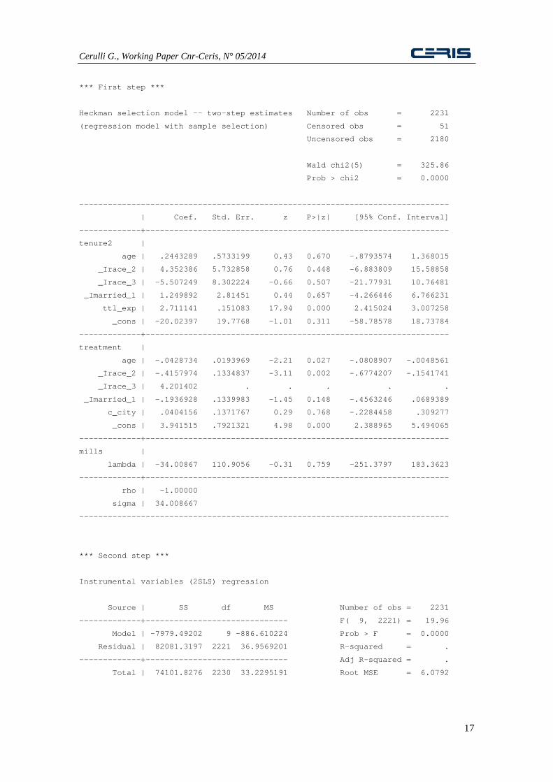
using "CT-IV" (Treatment endogeneity):

xi: ctreatreg wage treatment $xvars , graphrf ///

delta(10) hetero($xvarh) model(ct-iv) ct(tenure2) ci(1) ///

estype(twostep) iv_t(ttl_exp) iv_w(c_city)

Cnr-Ceris, N° 05/2014

.5547598 .0512772

4.124306 .3732158

521 .1145946

.001949 .0014024

.0000152 .0000128

13.34745 10.96255

--------------------------------------------------------------------------------

Response Function (Fig. 1), showing that

the relation is first weakly increasing and

then decreasing with a maximum around a

The relation is quite strongly significant



17

*** First step ***

Heckman selection model -- two-step estimates Number of obs = 2231

(regression model with sample selection) Censored obs = 51

Uncensored obs = 2180

Wald chi2(5) = 325.86

Prob > chi2 = 0.0000

------------------------------------------------------------------------------

| Coef. Std. Err. z P>|z| [95% Conf. Interval]

-------------+----------------------------------------------------------------

tenure2 |

age | .2443289 .5733199 0.43 0.670 -.8793574 1.368015

_Irace_2 | 4.352386 5.732858 0.76 0.448 -6.883809 15.58858

_Irace_3 | -5.507249 8.302224 -0.66 0.507 -21.77931 10.76481

_Imarried_1 | 1.249892 2.81451 0.44 0.657 -4.266446 6.766231

ttl_exp | 2.711141 .151083 17.94 0.000 2.415024 3.007258

_cons | -20.02397 19.7768 -1.01 0.311 -58.78578 18.73784

-------------+----------------------------------------------------------------

treatment |

age | -.0428734 .0193969 -2.21 0.027 -.0808907 -.0048561

_Irace_2 | -.4157974 .1334837 -3.11 0.002 -.6774207 -.1541741

_Irace_3 | 4.201402 . . . . .

_Imarried_1 | -.1936928 .1339983 -1.45 0.148 -.4563246 .0689389

c_city | .0404156 .1371767 0.29 0.768 -.2284458 .309277

_cons | 3.941515 .7921321 4.98 0.000 2.388965 5.494065

-------------+----------------------------------------------------------------

mills |

lambda | -34.00867 110.9056 -0.31 0.759 -251.3797 183.3623

-------------+----------------------------------------------------------------

rho | -1.00000

sigma | 34.008667

------------------------------------------------------------------------------

*** Second step ***

Instrumental variables (2SLS) regression

Source | SS df MS Number of obs = 2231

-------------+------------------------------ F( 9, 2221) = 19.96

Model | -7979.49202 9 -886.610224 Prob > F = 0.0000

Residual | 82081.3197 2221 36.9569201 R-squared = .

-------------+------------------------------ Adj R-squared = .

Total | 74101.8276 2230 33.2295191 Root MSE = 6.0792

18

------------------------------------------------------------------------------


-------------+-----------------------

treatment | 2.382129 28.81026 0.08 0.934

_ws_age | 2.483951 3.440528 0.72 0.470

Tw | .4324907 .1644757 2.63 0.009

T2w | -.006349 .0051065

T3w | .0000279 .0000414 0.67 0.500

age | -2.531013 3.396567

_Irace_2 | -1.90372 .732588

_Irace_3 | .9560915 1.293234 0.74 0.460

_Imarried_1 | -.7593091 .3741212

_cons | 105.4548 154.0347 0.68 0.494

------------------------------------------------------------------------------

Instrumented: treatment _ws_age Tw T2

Instruments: age _Irace_2 _Irace_3 _Imarried_1 probw _ps_age T_hatp

T_hat2p T_hat3p

We see that ATE becomes now positive

(2.38), but no longer significant. However,

the Dose Response Function (Fig. 2) set

Figure 2. Dose response function of “job tenure” on “wage”. Endogenous treatment case.

Cerulli G., Working Paper Cnr

------------------------------------------------------------------------------


----------------------------------------------------------------

treatment | 2.382129 28.81026 0.08 0.934 -54.11573 58.87999

_ws_age | 2.483951 3.440528 0.72 0.470 -4.263037 9.23094

Tw | .4324907 .1644757 2.63 0.009 .1099485 .7550328

.006349 .0051065 -1.24 0.214 -.0163629 .0036649

T3w | .0000279 .0000414 0.67 0.500 -.0000533 .0001091

2.531013 3.396567 -0.75 0.456 -9.191792 4.129767

1.90372 .732588 -2.60 0.009 -3.340349

_Irace_3 | .9560915 1.293234 0.74 0.460 -1.579983 3.492166

593091 .3741212 -2.03 0.043 -1.492973

_cons | 105.4548 154.0347 0.68 0.494 -196.6122 407.5218

------------------------------------------------------------------------------

Instrumented: treatment _ws_age Tw T2w T3w


T_hat2p T_hat3p

We see that ATE becomes now positive

(2.38), but no longer significant. However,

the Dose Response Function (Fig. 2) sets

out a pattern similar to the previous model,

with still a slight parabolic form, getting the

maximum at a dose level around 45.


Cnr-Ceris, N° 05/2014

------------------------------------------------------------------------------


-----------------------------------------

54.11573 58.87999

4.263037 9.23094

.1099485 .7550328

.0163629 .0036649

.0000533 .0001091

9.191792 4.129767

3.340349 -.4670908

1.579983 3.492166

1.492973 -.0256451

196.6122 407.5218

------------------------------------------------------------------------------


out a pattern similar to the previous model,

with still a slight parabolic form, getting the

maximum at a dose level around 45.



19

Of course, such results have to be taken

just as instructional, as we have no idea

about instruments’ goodness.

6. A MONTE CARLO EXPERIMENT

FOR TESTING CTREATREG’S

RELIABILITY

In this section we provide a Monte Carlo

experiment to check whether ctreatreg

complies with predictions from the theory

and to assess its correctness from a

computational point of view. The first step

is that of defining a data generating process

(DGP) as follows:

1 2

0 1 2

1 1 2

1 2

1[50 60 30 60 0]

0.1 0.2 0.3

0.3 0.6 0.3

0.4 0.6

= + + + + > = + + + = + + + = + +

w x x z a

y x x e

y x x e

t x x u

where we have assumed, for simplifying the

model, that e1=e0=e and:

1

2

(0;1) 100

(0;1) 100

(15,1)

(100,1)w

t

x U

x U

z N

z N

⋅ ⋅

∼

∼

∼

∼

with:

2 2, ,2 2

2 2,

( , ) ( ; )

1, 6.5, 0.8

σ σ σ ρ σ σσ σ

σ σ ρ

= =

= = =

∼

a a u a a u a u

u u

a u a u

a u N 0 Ω

Ω

Finally, we suppose that the correlation

between a and e0 can be either equal or

different from zero. In the latter case, w is

endogenous. Therefore, we assume the

following DGP6:

2 2

(0;1)

/(1 )

corr( ; )

0.0001

η γ

γ ρ ρρη

= + +

= −==

∼

e a v

v N

e a

When ρ=0 the model “ct-ols” would be

the appropriate one; otherwise, the model

“ct-iv” should be employed. By zw and zt,

we indicate the instrumental variable for w

and t, directly correlated with w and t

respectively, but (directly) uncorrelated

with y1 and y0.

Given these assumptions, the DGP is

completed by the potential outcome

equation yi = y0i + wi (y1i - y0i), generating

the observable outcome (or response) y.

The DGP is simulated 200 times using a

sample size of 10,000. For each simulation

we get a different data matrix (x1, x2, y, w, t,

zw, zt) on which we apply the two models

(“ct-ols” and “ct-iv”) implemented by

ctreatreg.

Case 1. Exogeneity

We start by assuming ρ=0, that is, zero

correlation between the error term of the

outcome equation (e) and the error term of

the selection equation (a). Under this

assumption, w is exogenous.

6 The coefficient γ is equal to (ρ2/(1- ρ2))-1/2 , where

ρ=corr(e0;a). To get this result put x=e and y=a. We

know that corr(x;y)=cov(x;y)/sd(x)sd(y). We can see

that, while var(y)=1 by assumption, var(x)=γ2+1.

Moreover,cov(x;y)=cov(η+γa+v;a)=cov(η+γa;a)+cov

(v;a)=cov(η+γa;a)=cov(γa;a)=γcov(a;a)=γvar(a)=γ.

Thus, ρ=γ/(γ2+1)-1/2, that implies that γ=(ρ2/(1- ρ2))-1/2.


20

Table 1. Mean test of ATE from Monte Carlo results using ctreatreg.

Exogenous selection is assumed.

Mean Std. Err. [95% Confidence Interval]

ATE (true value) 9.22 - - - ATE - CT-OLS 9.21 0.01 9.19 9.22 ATE - CT-IV 9.20 0.01 9.19 9.22 % BIAS of OLS 0.81 0.04 0.73 0.90 % BIAS of IV 0.86 0.04 0.77 0.94

Note: ρ=0. Number of observations 10,000. Number of simulations 200.

Moreover, we assume a strong correlation

between the selection and the dose

equation, as implied by a correlation

between a and u equal to 0.8. Results are

set out in Table 1. It is immediate to see

that the value of ATE obtained by the “ct-

ols” estimator is really close to the true

ATE (9.22) and that the confidence interval

at 5% of significance for this estimator

strictly contains that value. But also the

percentage bias of “ct-iv” is very low

(0.86%) and comparable with CT-OLS

(0.81%) and sufficient to imply that the 5%

of significance contains the true ATE even

in this case.

These results confirm what was expected,

thus showing that the option “ct-ols” of

ctreatreg behaves correctly. As a

conclusion, when the analyst assumes

exogeneity, he/she may reliably use

ctreatreg with the option “ct-ols”.

Case 2. Endogeneity

If we assume that ρ=0.7, that is, a high

positive correlation between the error term

of the outcome equation (e) and the error

term of the selection equation (a), then w

becomes endogenous. For the sake of

comparison, we still assume the same

strong correlation between the selection and

the dose equation (0.8).Table 2 shows that

results are - also in this case - coherent with

the theoretical predictions. Indeed, the

percentage bias of model “ct-ols” is rather

high and equal to around 18%, whereas the

bias of “ct-iv” is around 1%. Furthermore,

and more importantly, the 95% mean test

confidence interval for “ct-iv” contains the

true ATE.

Table 2. Mean test of ATE from Monte Carlo results using ctreatreg.

Endogenous selection is assumed.

Mean Std. Err. [95% Confidence Interval]

ATE (true value) 9.22 - - - ATE - CT-OLS 7.53 0.01 7.51 7.55 ATE - CT-IV 9.22 0.01 9.20 9.24 % BIAS of OLS 18.26 0.11 18.05 18.48 % BIAS of IV 1.28 0.07 1.15 1.41

Note: ρ=0.7. Number of observations 10,000. Number of simulations 200.


21

MODEL CT-OLS (under exogeneity) MODEL CT-IV (under endogeneity)

Figure 3. Graphical representation of the dose-response function using the ctreatreg option

CT-OLS and CT-IV under exogeneity and endogeneity respectively.

As expected, this implies that “ct-iv” is an

unbiased estimator in presence of selection

endogeneity, thus leading to a reliable

estimation of the true value of ATE.

Overall, these results confirm the

reliability of both the model and

ctreatreg by allowing for a trustful use

of this model and its related Stata

implementation either under selection

exogeneity or endogeneity. Finally, Fig. 3

plots the dose-response function along with

the 95% interval confidence lines for both

models. This is done by exploiting the

“graphdrf” option of ctreatreg. Results

clearly confirm our predictions.

7. CONCLUSION

The paper has presented ctreatreg, a

Stata module for estimating dose-response

functions through a regression approach

where: (i) treatment is continuous, (ii)

individuals may react heterogeneously to

observable confounders, and (iii) selection-

into-treatment may be endogenous.

Two estimation procedures are

contemplated by this routine: one based on

OLS under Conditional Mean Independence

(or CMI), and one based on Instrumental-

variables (IV), when assuming selection

endogeneity.

An application to real data, for testing in

an instructional example the impact of job

tenure on wages, has been set out. Finally,

in order to test the reliability of the

formulas and of their associated Stata

implementation, a Monte Carlo experiment

has been performed.

Monte Carlo results show that the

model’s formulas and the Stata routine

accompanying it are both reliable as

estimates consistently fit expected results.

01

02

030

40

Res

pons

e-fu

nctio

n

0 10 20 30 40 50 60 70 80 90 100

Dose (t)

ATE(t)95% confidence interval

Model: ct-ols

Outcome variable: outcome

Dose Response Function

010

2030

40

Res

pons

e-fu

nctio

n

0 10 20 30 40 50 60 70 80 90 100

Dose (t)

ATE(t)95% confidence interval

Model: ct-iv

Outcome variable: outcome

Dose Response Function


22

REFERENCES

Bia M., Mattei A. (2008) A Stata package

for the estimation of the dose–response

function through adjustment for the

generalized propensity score, The Stata

Journal, 8, 3, 354–373.

Bia M., Flores C. and Mattei A. (2011)

Nonparametric Estimators of dose-

response functions, CEPS/INSTEAD

Working Paper Series 2011-40,

CEPS/INSTEAD.

Cerulli G. (2012). “ivtreatreg: a new Stata

routine for estimating binary treatment

models with heterogeneous response to

treatment under observable and

unobservable selection”, CNR-Ceris

Working Papers, No. 03/12. Available at:

http://econpapers.repec.org/software/bocb

ocode/s457405.htm

Guardabascio B., Ventura M. (2013)

Estimating the dose-response function

through the GLM approach, MPRA Paper

45013, University Library of Munich,

Germany, revised 13 Mar 2013.

Forthcoming in: The Stata Journal.

Hirano K., Imbens G. (2004) The

propensity score with continuous

treatments. In Gelman, A. & Meng, X.L.

(Eds.), Applied Bayesian Modeling and

Causal Inference from Incomplete-Data

Perspectives (73-84). New York: Wiley.

Wooldridge J.M. (1997) On two stage least

squares estimation of the average

treatment effect in a random coefficient

model, Economics Letters, 56, 2,

129-133.

Wooldridge J.M. (2003) Further Results on

Instrumental Variables Estimation of

Average Treatment Effects in the

Correlated Random Coefficient Model,

Economics Letters, 79, 185-191.

Wooldridge J.M. (2010) Econometric

Analysis of cross section and panel data.

Chapter 18. Cambridge: MIT Press.

Royston P., Sauerbrei W., Becher H. (2010)

Modelling continuous exposures with a

'spike' at zero: a new procedure based on

fractional polynomials. Statistics in

Medicine, 29, 1219-27.

Royston P., Sauerbrei W. (2008)

Multivariable Model-building: A

Pragmatic Approach to Regression

Analysis Based on Fractional

Polynomials for Modelling Continuous

Variables. Wiley: Chichester.

Robertson, C., Boyle P., Hsieh C.C.,

Macfarlane G.J., Maisonneuve P. (1994)

Some statistical considerations in the

analysis of case-control studies when the

exposure variables are continuous

measurements, Epidemiology, 5,164-170.


23

Table A1. Stata help-file for ctreatreg.

help ctreatreg ---------------------------------------------------------------------------------------------------------------------- Title ctreatreg - Dose-Response model with "continuous" treatment, endogeneity and heterogeneous response to observable confounders Syntax ctreatreg outcome treatment [varlist] [if] [in] [weight], model(modeltype) ct(treat_level) [hetero(varlist_h) estype(model) iv_t(instrument_t) iv_w(instrument_w) delta(number) ci(number) graphate graphdrf conf(number) vce(robust) const(noconstant) head(noheader) beta] fweights, iweights, and pweights are allowed; see weight. Description ctreatreg estimates the dose-response function (DRF) of a given treatment on a specific target variable, within a model where units are treated with different levels. The DRF is defined as the “average treatment effect, given the level of the treatment t” (i.e. ATE(t)). The routine also estimates other “causal” parameters of interest, such as the average treatment effect (ATE), the average treatment effect on treated (ATET), the average treatment effect on non-treated (ATENT), and the same effects conditional on t and on the vector of covariates x.The DRF is approximated by a third degree polynomial function. Both OLS and IV estimation are available, according to the case in which the treatment is not or is endogenous. In particular, the implemented IV estimation is based on a Heckman bivariate selection model (i.e., type-2 tobit) for w (the yes/no decision to treat ……….a given unit) and t (the level of the treatment provided) in the first step, and a 2SLS estimation for the outcome (y) equation in the second step. The routine allows also for a graphical representation of results. Options model(modeltype) specifies the treatment model to be estimated, where modeltype must be one of the following two models: "ct-ols", "ct-iv". it is always required to specify one model. ct(treat_level) specifies the treatment level (or dose). This variable takes values in the [0;100] interval, where 0 is the treatment level of non-treated units. The maximun dose is thus 100. hetero(varlist_h) specifies the variables over which to calculate the idiosyncratic Average Treatment Effect ATE(x), ATET(x) and ATENT(x), where x=varlist_h. It is optional for all models. When this option is not specified, the command estimates the specified model without heterogeneous average effect. Observe that varlist_h should be the same set or a subset of the variables specified in varlist. Observe however that only numerical variables may be considered. estype(model) specifies which type of estimation method has to be used for estimating the type-2 tobit model in the endogenous treatment case. Two choices are available: "twostep" implements a Heckman two-step procedure; "ml" implements a maximum-likelihood estimation. This option is required only for "ct-iv". iv_t(instrument_t) specifies the variable to be used as instrument for the continuous treatment variable t in the type-2 tobit model. This option is required only for "ct-iv". iv_w(instrument_w) specifies the variable to be used as instrument for the binary treatment variable w in the type-2 tobit model. This option is required only for "ct-iv". delta(number) identifies the average treatment effect between two states: t and t+delta. For any reliable delta, we can obtain the response function ATE(t;delta)=E[y(t)-y(t+delta)]. ci(number) sets the significant level for the dose-response function, where number may be 1, 5 or 10. graphate allows for a graphical representation of the density distributions of ATE(x;t) ATET(x;t) and ATENT(x;t). It is optional for all models and gives an outcome only if variables into hetero() are specified. graphdrf allows for a graphical representation of the Dose Response Function (DRF) and of its derivative. It plots also the 95% confidence interval of the DRF over the dose levels. vce(robust) allows for robust regression standard errors. It is optional for all models. beta reports standardized beta coefficients. It is optional for all models. const(noconstant) suppresses regression constant term. It is optional for all models. conf(number) sets the confidence level equal to the specified number. The default is number=95. modeltype_options description -------------------------------------------------------------------------------------------------------------------- Model ct-ols Control-function regression estimated by ordinary least squares ct-iv IV regression estimated by Heckman bivariate selection model and 2SLS -------------------------------------------------------------------------------------------------------------------- ctreatreg creates a number of variables: _ws_varname_h are the additional regressors used in model's regression when hetero(varlist_h) is specified. _ps_varname_h are the additional instruments used in model's regression when hetero(varlist_h) is specified in model "ct-iv". ATE(x;t) is an estimate of the idiosyncratic Average Treatment Effect. ATET(x;t) is an estimate of the idiosyncratic Average Treatment Effect on treated. ATENT(x;t) is an estimate of the idiosyncratic Average Treatment Effect on Non-Treated.


24

ATE(t) is an estimate of the dose-response function. ATET(t) is the value of the dose-response function in t>0. ATENT(t) it is the value of the dose-response function in t=0. probw is the predicted probability from the Heckman selection model (estimated only for model "ct-iv"). mills is the predicted Mills' ratio from the Heckman selection model (estimated only for model "ct-iv"). t is a copy of the treatment level variable, but only in the sample considered. t_hat is the prediction of the level of treatment from the Heckman bivariate selection model (estimated only for model "ct-iv"). der_ATE_t is the estimate of the derivative of the dose-response function. std_ATE_t is the standardized value of the dose-response function. std_der_ATE_t is the standardized value of the derivative of the dose-response function. Tw, T2w, T3w are the three polynomial factors of the dose-response function. T_hatp, T2_hatp, T3_hatp are the three instruments for the polynomial factors of the dose-response function when model "ct-iv" is used. ctreatreg returns the following scalars: r(N_tot) is the total number of (used) observations. r(N_treated) is the number of (used) treated units. r(N_untreated) is the number of (used) untreated units. r(ate) is the value of the Average Treatment Effect. r(atet) is the value of the Average Treatment Effect on Treated. r(atent) is the value of the Average Treatment Effect on Non-treated. Remarks The variable specified in treatment has to be a 0/1 binary variable (1 = treated, 0 = untreated). The standard errors for ATET and ATENT may be obtained via bootstrapping. When using the option ct-iv in modeltype(), be sure that the number of variables included in hetero() is less than the number of variables included in varlist. This is because otherwise instruments are too much correlated and some emerging collinearity prevent to identify the estimates. For instance, when six covariates are specified in varlist, at most five are to be put into hetero().

Working Paper Cnr-Ceris

ISSN (print): 1591-0709 ISSN (on line): 2036-8216

Download

www.ceris.cnr.it/index.php?option=com_content&task=section&id=4&Itemid=64

Hard copies are available on request,

please, write to:

Cnr-Ceris

Via Real Collegio, n. 30

10024 Moncalieri (Torino), Italy

Tel. +39 011 6824.911 Fax +39 011 6824.966

[email protected] www.ceris.cnr.it

Copyright © 2014 by Cnr–Ceris

All rights reserved. Parts of this paper may be reproduced with the permission

of the author(s) and quoting the source.

mailto:[email protected]

cover new impa ceris 2010 - Boston Collegefm · Cerulli G., Working Paper Cnr-Ceris, N° 05/2014 ....

Documents

Transcript of cover new impa ceris 2010 - Boston Collegefm · Cerulli G., Working Paper Cnr-Ceris, N° 05/2014 ....