CoVaR∗

Tobias Adrian†

Federal Reserve Bank of New YorkMarkus K. Brunnermeier‡

Princeton University

This Version: September 10, 2014

Abstract

We propose a measure for systemic risk, ∆CoVaR, defined as the conditional value at risk(CoVaR) of the financial system conditional on an institution being under distress in excess ofthe CoVaR conditional on the median state of the institution. Our ∆CoVaR estimates show thatcharacteristics such as leverage, size, maturity mismatch, and asset price booms significantlypredict systemic risk contribution. We provide out-of-sample forecasts of a countercyclical,forward-looking measure of systemic risk and show that the 2006Q4 value of this measure wouldhave predicted more than one third of realized ∆CoVaR during the financial crisis.

Keywords: Value at Risk, Systemic Risk, Risk Spillovers, Financial Architecture

JEL classification: G01, G10, G18, G20, G28, G32, G38

∗Special thanks go to Evan Friedman, Daniel Green, Hoai-Luu Nguyen, Daniel Stackman and Christian Wolffor outstanding research assistance. The authors also thank Paolo Angelini, Gadi Barlevy, Rene Carmona, StephenBrown, Robert Engle, Mark Flannery, Xavier Gabaix, Paul Glasserman, Beverly Hirtle, Jon Danielson, John Kambhu,Arvind Krishnamurthy, Burton Malkiel, Ulrich Muller, Maureen O’Hara, Andrew Patton, Matt Pritsker, MattRichardson, Jean-Charles Rochet, Jose Scheinkman, Jeremy Stein, Kevin Stiroh, Rene Stulz, and Skander Vanden Heuvel for feedback, as well as seminar participants at numerous universities, central banks, and conferences. Weare grateful for support from the Institute for Quantitative Investment Research Europe. Brunnermeier acknowledgesfinancial support from the Alfred P. Sloan Foundation. The paper first appeared as Federal Reserve Bank of NewYork Staff Report 348 on September 5, 2008. The views expressed in this paper are those of the authors and do notnecessarily represent those of the Federal Reserve Bank of New York or the Federal Reserve System.†Federal Reserve Bank of New York, Capital Markets Function, Research and Statistics Group, 33 Liberty Street,

New York, NY 10045, tobias.adrian@ny.frb.org, http://nyfedeconomists.org/adrian.‡Princeton University, Bendheim Center for Finance, Department of Economics, Princeton, NJ 08540-5296, NBER,

CEPR, CESIfo, markus@princeton.edu, http://www.princeton.edu/~markus.

1 Introduction

In times of financial crisis, losses spread across financial institutions, threatening the financial

system as a whole.1 The spreading of distress gives rise to systemic risk—the risk that the interme-

diation capacity of the entire financial system is impaired, with potentially adverse consequences

for the supply of credit to the real economy. In systemic financial events, spillovers across institu-

tions can arise from direct contractual links and heightened counterparty credit risk, or can occur

indirectly through price effects and liquidity spirals. As a result of these spillovers, the measured

comovement of institutions’ assets and liabilities tends to rise above and beyond levels purely jus-

tified by fundamentals. Systemic risk measures capture the potential for the spreading of financial

distress across institutions by gauging this increase in tail comovement.

The most common measure of risk used by financial institutions—the value at risk (VaR)—

focuses on the risk of an individual institution in isolation. For example, the q%-VaRi is the

maximum loss of institution i at the q%-confidence level.2 However, a single institution’s risk

measure does not necessarily reflect its contribution to overall systemic risk, for several reasons.

Some institutions are individually systemic—they are so interconnected and large that they can

cause negative risk spillover effects on others. Similarly, several smaller institutions may be systemic

as part of a herd. In addition to the cross-sectional dimension, systemic risk also has a time-series

dimension. Systemic risks typically build in times of low volatility, and materialize during crises.

A good systemic risk measure should capture this build-up. This means that high-frequency risk

measures that rely mostly on contemporaneous price movements are potentially misleading.

In this paper, we propose a new reduced-form measure of contributions to systemic risk—the

∆CoVaR. This new measure captures tail dependency and includes negative spillover dynamics in

times of crises. We also project the ∆CoVaR on lagged institutional characteristics (in particular

size, leverage, and maturity mismatch) and conditioning variables (in particular market volatility

and fixed income spreads). This procedure gives a forward-looking systemic risk contribution

measure—the forward -∆CoVaR— which captures the build-up of systemic risk in tranquil times.

To emphasize the systemic nature of our risk measure, we add to existing risk measures the

1Examples include the 1987 equity market crash, which was started by portfolio hedging of pension funds and ledto substantial losses of investment banks; the 1998 crisis, which was started with losses of hedge funds and spilledover to the trading floors of commercial and investment banks; and the 2007-09 crisis, which spread from SIVs tocommercial banks and on to investment banks and hedge funds. See e.g. Brady (1988), Rubin, Greenspan, Levitt,and Born (1999), Brunnermeier (2009), and Adrian and Shin (2010a).

2See Kupiec (2002) and Jorion (2006) for detailed overviews.

1

prefix “Co,” for conditional. We focus primarily on CoVaR, where institution i’s CoVaR relative

to the system is defined as the VaR of the whole financial sector conditional on institution i being

in a particular state, such as distress or the median state.3 The difference between the CoVaR

conditional on the distress of an institution and the CoVaR conditional on the “normal” state

of the institution, ∆CoVaR, captures the contribution of a particular institution, in a non-causal

sense, to the overall systemic risk. ∆CoVaR is a statistical tail dependency measure, and so is best

viewed as a useful reduced-form analytical tool capturing (tail) comovements.

The systemic risk contribution measure ∆CoVaR differs from an individual institution’s risk

measure VaR. Figure 1 shows this for the leading financial institutions in the US. Hence, it is not

sufficient to regulate financial institutions purely based on the risk of institutions in isolation as it

can lead to excessive risk-taking along systemic risk dimension.

WB

WFC

JPM

BAC

C

MER

BSC

MS

LEH

GS

AIG

MET

PRU

FNMFRE

10

20

30

40

50

∆C

oV

aR

60 80 100 120 140 160Institution VaR

Commercial Banks Investment Banks

Insurance Companies GSEs

Figure 1: VaR and ∆CoVaR. The scatter plot shows the weak link between institutions’ risk in isolation,

measured by VaRi (x-axis), and institutions’ contribution to system risk, measured by ∆CoVaRi (y-axis).

The VaRi and ∆CoVaRi are unconditional 99% measures estimated as of 2006Q4 and are reported in

quarterly percent returns for merger adjusted entities. ∆CoVaRi is the difference between the financial

system’s VaR conditional on firm i′s distress and the financial system’s VaR conditional on firm i′s median

state. The institution names are listed in Appendix D.

3Under many distributional assumptions (such as the assumption that shocks are conditionally Gaussian), the VaRof an institution is proportional to the variance of the institution, and the CoVaR of an institution is proportionalto the covariance of the financial system and the individual institution.

2

∆CoVaR is directional. Reverting the conditioning allows one to answer which institutions

are most at risk should a financial crisis occur (as opposed to which institutions contributes to it

the most). ∆CoVaR is general enough to capture directional tail dependency from institution to

institution across the whole financial network.

So far, we have deliberately not specified how to estimate ∆CoVaR, since there are many

possible ways. In this paper, we primarily use quantile regressions, which are appealing for their

simplicity. Since we want to capture all forms of risk, including not only the risk of adverse asset

price movements, but also funding liquidity risk, our estimates of ∆CoVaR are based on weekly

equity returns of all publicly traded financial institutions. However, ∆CoVaR can also be estimated

using methods such as GARCH models, as we show in the appendix.

We calculate unconditional and conditional measures of ∆CoVaR using the full length of avail-

able data. We use weekly data from 1971Q1 to 2013Q2 for all publicly traded commercial banks,

broker-dealers, insurance companies, and real estate companies. We also verify for financial firms

that are listed since 1926 that a longer estimation window does not materially alter the systemic

risk contribution estimates. We model the variation of ∆CoVaR as a function of state variables

that capture the evolution of tail risk dependence over time. These state variables include the

slope of the yield curve, the aggregate credit spread, and realized equity market volatility. We first

estimate ∆CoVaR conditional on the state variables. In a second step we use panel regressions,

and relate these time-varying ∆CoVaRs—in a predictive, Granger causal sense—to measures of

each institution’s characteristics like maturity mismatch, leverage, size, and asset valuations. We

find relationships that are in line with theoretical predictions: higher leverage, more maturity mis-

match, larger size, and higher valuations forecast higher systemic risk contributions across financial

institutions.

Systemic risk monitoring should be based on forward-looking risk measures. We propose such

a forward-looking measure—the forward-∆CoVaR. This forward-∆CoVaR has countercyclical fea-

tures, reflecting the buildup of systemic risk in good times, and the realization of systemic risk

in crises. Crucially, the countercyclicality of our forward measure is a result, not an assump-

tion. Econometrically, we construct the forward -∆CoVaR by regressing time-varying ∆CoVaRs

on lagged institutional characteristics and common risk factors. We estimate forward -∆CoVaR

out-of-sample. Consistent with the “volatility paradox”—the notion that low volatility environ-

3

ments breed the build up of systemic risk—the forward -∆CoVaR is negatively correlated with the

contemporaneous ∆CoVaR. We also demonstrate that the forward -∆CoVaR has out of sample pre-

dictive power for realized ∆CoVaR in tail events. In particular, the forward -∆CoVaR estimated

using data through the end of 2006 predicts a substantial fraction of the cross-sectional dispersion

in realized ∆CoVaR during the financial crisis of 2007-08. The forward -∆CoVaR can thus be

used to monitor the buildup of systemic risk in a forward-looking manner. It remains, however,

a reduced-form measure, and so does not causally allocate systemic risk contributions to different

financial institutions.

Outline. The remainder of the paper is organized in five sections. We first present a review

of the related literature. Then, in Section 3, we present the methodology, define ∆CoVaR and

discuss its properties. In Section 4, we outline the estimation method via quantile regressions. We

allow for time variation in the ∆CoVaRs by modeling them as a function of various state variables

and present estimates of these time varying ∆CoVaRs. Section 5 then introduces the forward -

∆CoVaR, illustrates its countercyclicality and demonstrates that institutional characteristics such

as size, leverage, and maturity mismatch can predict systemic risk contribution in the cross section

of institutions. We conclude in Section 6.

2 Literature Review

Our co-risk measure is motivated by theoretical research on externalities across financial institutions

that give rise to amplifying liquidity spirals and persistent distortions. It also relates closely to

recent econometric work on contagion and spillover effects.

2.1 Theoretical Background on Systemic Risk

Spillovers can give rise to excessive risk taking and leverage in the run-up phase to a crisis. Spillovers

in the form of externalities arise when individual institutions take potential fire-sale prices as given,

while fire-sale prices are determined jointly by all institutions. In an incomplete market setting,

this pecuniary externality leads to an outcome that is not even constrained Pareto efficient. This

result was derived in a banking context in Bhattacharya and Gale (1987) and a general equilibrium

incomplete market setting by Stiglitz (1982) and Geanakoplos and Polemarchakis (1986). Prices

4

can also affect borrowing constraints. These externality effects are studied within an international

finance context by Caballero and Krishnamurthy (2004), and most recently shown in Lorenzoni

(2008), Acharya (2009), Stein (2009), and Korinek (2010). Runs on financial institutions are

dynamic co-opetition games and lead to externalities, as does banks’ liquidity hoarding. While

hoarding might be microprudent from a single bank’s perspective it need not be macroprudent

(fallacy of the commons). Finally, network effects can also lead to spillover effects, as emphasized

by Allen, Babus, and Carletti (2010).

Procyclicality occurs because risk measures tend to be low in booms and high in crises. Brun-

nermeier and Sannikov (2014) coined the term “volatility paradox”. The margin/haircut spiral

and precautionary hoarding behavior, outlined in Brunnermeier and Pedersen (2009) and Adrian

and Boyarchenko (2012), lead financial institutions to shed assets at fire-sale prices. Adrian and

Shin (2010b), Gorton and Metrick (2010), and Adrian, Etula, and Muir (2010) provide empirical

evidence for the margin/haircut spiral. Borio (2004) is an early contribution that discusses a policy

framework to address margin/haircut spirals and procyclicality.

2.2 Other Systemic Risk Measures

∆CoVaR, of course, is not the only systemic risk measure. Huang, Zhou, and Zhu (2010) develop a

systemic risk indicator that measures the price of insurance against systemic financial distress from

credit default swap (CDS) prices. Acharya, Pedersen, Philippon, and Richardson (2010) focus

on high-frequency marginal expected shortfall as a systemic risk measure. Like our “Exposure-

∆CoVaR”—to be defined later—they switch the conditioning and address the question of which

institutions are most exposed to a financial crisis as opposed to which institution contributes

most to a crisis. Importantly, their analysis focuses on a cross-sectional comparison of financial

institutions and does not address the problem of procyclicality that arises from contemporaneuous

risk measurement. In other words, they do not address the stylized fact that risk builds up in the

background during boom phases characterized by low volatility and materializes only in crisis times.

Acharya, Engle, and Richardson (2012) develop the closely related SRISK measure which calculates

capital shortfall of individual institutions conditional on market stress. Billio, Getmansky, Lo, and

Pelizzon (2010) propose a systemic risk measure that relies on Granger causality among firms.

Giglio (2011) uses a nonparametric approach to derive bounds of systemic risk from CDS prices. A

5

number of recent papers have extended the ∆CoVaR method and applied it to additional financial

sectors. For example, Adams, Fuss, and Gropp (2010) study risk spillovers among financial sectors;

Wong and Fong (2010) estimate ∆CoVaR for the CDS of Asia-Pacific banks; Gauthier, Lehar,

and Souissi (2012) estimate systemic risk exposures for the Canadian banking system. Another

important strand of the literature, initiated by Lehar (2005) and Gray, Merton, and Bodie (2007),

uses contingent claims analysis to measure systemic risk. Bodie, Gray, and Merton (2007) develop

a policy framework based on the contingent claims. Segoviano and Goodhart (2009) use a related

approach to measure risk in the global banking system.

2.3 The Econometrics of Tail Risk and Contagion

The ∆CoVaR measure is also related to the literature on volatility models and tail risk. In a seminal

contribution, Engle and Manganelli (2004) develop CAViaR, which uses quantile regressions in

combination with a GARCH model to capture the time varying tail behavior of asset returns.

Manganelli, Kim, and White (2011) study a multivariate extension of CAViaR, which can be used

to generate a dynamic version of CoVaR. Brownlees and Engle (2010) propose methodologies to

estimate systemic risk measures using GARCH models.

The ∆CoVaR measure can additionally be related to an earlier literature on contagion and

volatility spillovers (see Claessens and Forbes (2001) for an overview). The most common method

to test for volatility spillovers is to estimate multivariate GARCH processes. Another approach

is to use multivariate extreme value theory. Hartmann, Straetmans, and de Vries (2004) develop

a contagion measure that focuses on extreme events. Danielsson and de Vries (2000) argue that

extreme value theory works well only for very low quantiles.

Since the current paper was first circulated in 2008, a literature on alternative estimation

approaches for CoVaR has been emerging. CoVaR is estimated using multivariate GARCH by

Girardi and Tolga Ergun (2013) (see also our Appendix B). Mainik and Schaanning (2012) and Oh

and Patton (2013) use copulas. Bayesian inference for CoVaR estimation is proposed by Bernardi,

Gayraud, and Petrella (2013). Bernardi, Maruotti, and Petrella (2013) and Cao (2013) make

distributional assumptions about shocks and employ maximum likelihood estimators. Extensions

of the quantile regression approach for CoVaR can be found in Castro and Ferrari (2014).

6

3 CoVaR Methodology

3.1 Definition of ∆CoVaR

Recall that VaRiq is implicitly defined as the q% quantile, i.e.,

Pr(Xi ≤ VaRi

q

)= q%,

where Xi is the loss of institution i for which the VaRiq is defined. Defined like this, VaRi

q is

typically a positive number when q > 50, in line with the commonly used sign convention. Hence

more risk corresponds to a greater VaRiq. We define Xi as the “return loss”.

Definition 1 We denote by CoVaRj|C(Xi)q the VaR of institution j (or the financial system) con-

ditional on some event C(Xi)

of institution i. That is, CoVaRj|C(Xi)q is implicitly defined by the

q%-quantile of the conditional probability distribution:

Pr

(X j|C

(Xi)≤ CoV aRj|C(Xi)

q

)= q%.

We denote institution i’s contribution to j by

∆CoV aRj|iq = CoVaRj|Xi=VaRi

qq − CoVaR

j|Xi=VaRi50

q ,

and in dollar terms

∆$CoV aRj|iq =$Sizei ·∆CoV aRj|iq .

In our benchmark specification j will be the losses of the portfolio of all financial institutions.

Conditioning. To obtain CoVaR we typically condition on an event C that is equally likely

across institutions. Usually C is institution i’s loss being at or above its VaRiq level, which—by

definition—occurs with likelihood (1− q) %. Importantly, this implies that the likelihood of the

conditioning event is independent of the riskiness of i’s strategy. If we were to condition on a

particular return level (instead of a quantile), then more conservative (i.e., less risky) institutions

could have a higher CoVaR simply because the conditioning event would be a more extreme event

for less risky institutions.

7

∆CoVaR captures the increase in CoVaR as one shifts the conditioning event from the median

return of institution i to the adverse VaRiq (with equality). ∆CoVaR measures the “tail depen-

dency” between two random variables. Note that, for jointly normally distributed random variables,

∆CoVaR is related to the correlation coefficient, while CoVaR corresponds to a conditional vari-

ance. Conditioning by itself reduces the variance, while conditioning on adverse events increases

expected losses.

∆$CoVaR takes the size of institution i into account in order to compare the systemic risk

contributions across institutions. For the purpose of this paper we capture the size with the market

equity of the institution. Financial regulators (and in an earlier draft of our paper we) use total

assets for the return as well as the size definition.4

CoES. One attractive feature of CoVaR is that it can be easily adapted for other “corisk-

measures.” An example of this is the co-expected shortfall, CoES. Expected shortfall, the expected

loss conditional on a VaR event, has a number of advantages relative to VaR5, and these consider-

ations extend to CoES. CoESj|iq may be defined as the expected loss for institution j conditional

on its losses exceeding CoVaRj|iq , and ∆CoES

j|iq analogously is just CoES

j|iq − CoES

j|i50 .

3.2 The Economics of Systemic Risk

Systemic risk has a time-series and a cross-sectional dimension. In the time-series, systemic risk

builds up during credit booms when contemporaneously measured risk is low. This buildup of

systemic risk during times of low measured risk gives rise to a “volatility paradox.” Hence, contem-

poraneous systemic risk measures are not suited to capture the buildup component of systemic risk.

In Section 5, we construct a “forward-∆CoVaR” that avoids the “procyclicality pitfall” by estimat-

ing the relationship between current firm characteristics and future tail dependency, as proxied by

∆CoVaRj|iq,t.

The cross-sectional component of systemic risk relates to the spillover effects that amplify initial

adverse shocks in times of crises. The contemporaneous ∆CoVaRi measures the tail dependency and

4For multi-strategy institutions and funds, it might make sense to calculate the ∆CoVaR for each strategy sseparately and obtain ∆$CoV aR

j|iq =

∑s Size

s,i ·∆CoV aRj|sq . This ensures that mergers and carve-outs of strategies

do not impact their overall systemic risk contribution measure, and also improves the cross-sectional comparison.5In particular, the VaR is not subadditive and does not take distributional aspects within the tail into account.

However, these concerns are mostly theoretical in nature as the exact distribution within the tails is difficult toestimate.

8

captures both spillover and common exposure effects. It captures how much an institution adds to

the overall risk of the financial system. The spillover effects can be direct, through contractual links

among financial institutions. Indirect spillover effects, however, are quantitatively more important.

Selling off assets can lead to mark-to-market losses for all market participants who hold a similar

exposure. Moreover, the increase in volatility might tighten margins and haircuts forcing other

market participants to delever as well (margin spiral). This can lead to crowded trades which

increases the price impact even further, see e.g. Brunnermeier and Pedersen (2009). Many of

these spillovers are externalities. That is, when taking on the initial position with low market

liquidity funded with short-term liabilities—i.e. with high liquidity mismatch— individual market

participants do not internalize that subsequent individually optimal response in times of crises

will impose (pecuniary) externalities on others. As a consequence, the initial risk taking is often

excessive in the run-up phase, which generates the first component of systemic risk.

3.3 Tail Dependency versus Causality

∆CoVaRj|iq is a statistical tail-dependency measure and does not necessarily correctly capture

externalities or spillover effects, for several reasons. First, the externalities are typically not fully

observable in equilibrium, since other institutions might reposition themselves in order to reduce the

impact of the externalities. Second, ∆CoVaRj|iq also captures the common exposure to exogenous

aggregate macroeconomic risk factors.

More generally, causal statements can only be made within a specific model. Here, we consider

for illustrative purposes a simple stylized financial system that can be split into two groups, in-

stitutions of type i and of type j. There are two latent independent risk factors, ∆Zi and ∆Zj .

We conjecture that institutions of type i are directly exposed to the sector specific shock ∆Zi, and

indirectly exposed to ∆Zj due to spillover effects. The assumed data generating process of returns

for type i institutions −Xit+1 = ∆N i

t+1/Nit is

−Xit+1 = µi (·) + σii (·) ∆Zit+1 + σij (·) ∆Zjt+1, (1)

where the short-hand notation (·) indicates that the (geometric) drift and volatility loadings are

functions of the following state variables(Mt, L

it, L

jt , N

it , N

jt

): the state of the macro-economy, Mt,

the leverage and liquidity mismatch of type i institutions, Lit, and of type j institutions, Ljt , as well

9

as the net worth levels N it and N j

t . Leverage Lit is a choice variable and presumably, for i type

institutions, increases the loading to the own latent risk factor ∆Zit+1. One would also presume

that the exposure of i type institutions to ∆Zjt+1 due to spillovers, σij (·), is increasing in the own

leverage, Lit, and others’ leverage, Ljt .

Analogously, for institutions of type j, we propose the following data generating process:

−Xjt+1 = µj (·) + σjj (·) ∆Zjt+1 + σji (·) ∆Zit+1. (2)

As the two latent shock processes ∆Zit+1 and ∆Zjt+1 are unobservable, the empirical analysis

starts with the following two of reduced form equations:6

−Xit+1 = µi (·)− σij (·)Xj

t+1 + σii (·) ∆Zit+1, (3)

−Xjt+1 = µj (·)− σji (·)Xi

t+1 + σjj (·) ∆Zjt+1. (4)

Consider an adverse shock ∆Zit+1 < 0. This shock lowers −Xit+1 by σiit ∆Zit+1. First round spillover

effects also reduce the others’ return −∆Xjt+1 by σjit σ

iit ∆Zit+1. Lower −∆Xj

t+1, in turn, lowers

−∆Xit+1 by σijt σ

jit σ

iit ∆Zit+1 due to second round spillover effects. The argument goes on through

third, fourth etc. round effects. When a fixed point is ultimately reached, we obtain the volatility

loadings of the initially proposed data generating process σiit =∑∞

n=0(σijt σjit )nσiit =

σiit

1−σijt σ

jit

.

Similarly, σijt =∑∞

n=0(σijt σjit )nσijt σ

jjt =

σijt σ

jjt

1−σijt σ

jit

. Analogously, replacing i with j and vice versa,

we obtain σjjt and σjit . That is, this reasoning allows one to link reduced form σs to primitive σs.

Gaussian case. An explicit formula can be derived for the special case in which all innovations

∆Zit+1 and ∆Zjt+1 are jointly Gaussian distributed. In this case

∆CoV aRj|iq,t = ∆V aRiqt · β

ijt (5)

= −(Φ−1 (q)

)2 Covt [Xit+1, X

jt+1

]∆V aRiq,t

= −Φ−1(q)σjtρijt , (6)

6The location scale model outlined in Appendix A falls in this category, with µj(Mt), σji = const., σjj(Mt, X

it+1),

and the error term distributed i.i.d. with zero mean and unit variance. Another difference relative to this model arelosses in return space (not net worth in return space) as the dependent variable.

10

where βijt =Covt[Xi

t+1,Xjt+1]

V art[Xit+1]

=σiit σ

jit +σij

t σjjt

σiit σ

iit +σij

t σijt

is the OLS regression coefficient of reduced form Equa-

tion (4). Note that in the Gaussian case the OLS and median quantile regression coefficient are

the same. Φ (·) is the standard Gaussian cdf, σjt is the standard deviation of N jt+1/N

jt , and ρijt

the correlation coefficient between N it+1/N

it and N j

t+1/Njt . The Gaussian setting results in a nice

analytical solution, but its tail properties are less desirable than those of more general distributional

specifications.

3.4 CoVaR, Exposure-CoVaR, Network-CoVaR

The superscripts j or i can refer to losses of individual institutions or of a portfolio of institutions.

∆CoVaRj|iq is directional. That is, the ∆CoVaR

system|iq of the system conditional on institution i

is not equal to ∆CoVaRi|systemq of institution i conditional on the financial system being in crisis.

The conditioning radically changes the interpretation of the systemic risk contribution measure.

In this paper we consider primarily the direction of conditioning ∆CoVaRsystem|iq . It stresses how

much more risky the system is in states of the world in which institution i is in distress relative to

its normal times. Specifically,

∆CoVaRsystem|iq = CoVaR

system|Xi=VaRiq

q − CoVaRsystem|Xi=VaRi

50q .

Exposure-∆CoVaR. For risk management questions, it is sometimes useful to compute the

opposite conditioning. We can derive CoVaRj|system, which answers the question of which institu-

tions are most at risk should a financial crisis occur. ∆CoVaRj|system, which we label “Exposure-

∆CoVaR”, reports institution j’s increase in value at risk in the case of a financial crisis. In other

words, the Exposure-∆CoVaR is a measure of an individual institution’s exposure to system wide

distress, and is similar to the stress tests performed by individual institutions or regulators.

The importance of the direction of the conditioning is probably best illustrated with the follow-

ing example. Consider a financial institution (perhaps a venture capitalist) with returns subject

to substantial idiosyncratic noise. If the financial system overall is in significant distress, then

this institution is also likely to face difficulties, so its Exposure-∆CoVaR is high. At the same

time, conditioning on this particular institution being in distress does not materially impact the

probability that the wider financial system is in distress (due to the large idiosyncratic component

of the returns), and so ∆CoVaR is low. In this example the Exposure-∆CoVaR would send the

11

wrong signal about systemicness, were it to be viewed as an indicator of such.

Network-∆CoVaR. Finally, whenever j and i in CoVaRj|i refer to individual institutions, we

talk of a “Network -∆CoVaR”. In this case we can study of tail dependency across a whole financial

network.

To simplify notation we sometimes drop the subscript q when it is not necessary to specify the

confidence level of the risk measures. Also, for the benchmark ∆CoVaRsystem|i we often write only

∆CoVaRi. Later we will also introduce a time varying systemic risk contribution measure and add

a subscript t to denote time ∆CoVaRsystem|iq,t .

3.5 Properties of ∆CoVaR

Clone Property. Our ∆CoVaR definition satisfies the desired property that, after splitting one

large individually systemic institution into n smaller clones, the CoVaR of the large institution (in

return space) is exactly the same as the CoVaRs of the n clones. Put differently, conditioning on

the distress of a large systemic institution is the same as conditioning on one of the n clones. This

property of course also holds for the Gaussian case, as can be seen from Equation (6). Both the

covariance and the ∆VaR are divided by n, leaving ∆CoVaRj|iq,t unchanged.

Systemic as Part of a Herd. Consider a large number of small financial institutions which

hold similar positions, and are funded in a similar way—in short, they are exposed to the same

factors. Now, if only one of these institutions falls into distress, then this will not necessarily cause

a systemic crisis. However, if the distress is due to a common factor, then the other institutions

will also be in distress. Overall, the institutions are systemic as part of a herd. Each individual

institution’s co-risk measure should capture this notion of being “systemic as part of a herd”, even

in the absence of a direct causal link. The ∆CoVaR measure achieves exactly that. Moreover,

when we estimate ∆CoVaR, we control for lagged state variables that capture variation in tail risk

not directly related to the financial system risk exposure. This discussion connects naturally with

the clone property: If we split a systemically important institution into n clones, then each clone

is systemic as part of the herd. The ∆CoVaR of each clone is the same as that of the original

institution, capturing the intuition of systemic risk in a herd.

12

Endogeneity of Systemic Risk. Note that each institution’s ∆CoVaR is endogenous and de-

pends on other institutions’ risk taking. Hence, imposing a regulatory framework that forces insti-

tutions to lower their leverage and liquidity mismatch, Li, lowers reduced form σi·(·) in Equations

(1, 2), and spillover effects captured in primitive σi·(·) in Equations (3, 4).

To the extent that a regulatory framework tries to internalize externalities, ∆CoVaR measures

change. ∆CoVaR is an equilibrium concept which adapts to changing environments and provides

incentives for institutions to reduce their exposure to risk if other institutions load excessively on it.

Overall, we believe that ∆CoVaR can be a useful reduced-form analytical tool, but should neither

serve as an explicit target for regulators, nor guide the setting of systemic taxes.7

4 ∆CoVaR Estimation

In this section we outline the estimation of ∆CoVaR. In Section 4.1 we start with a discussion

of alternative estimation approaches and then in Section 4.2 present the quantile regression based

estimation method that we use in this paper. We go on to describe estimation of the time-varying,

conditional ∆CoVaR in Section 4.3. Details on the econometrics are given in Appendix A and

robustness checks including the GARCH estimation of ∆CoVaR are provided in Appendix B.

Section 4.4 provides estimates of ∆CoVaR and discusses properties of the estimates.

4.1 Alternative Empirical Approaches

The CoVaR measure can be computed in various ways. Our main estimation approach relies on

quantile regressions, as we explain in Sections 4.2 and 4.3. Quantile regressions are a numerically

efficient way to estimate CoVaR. Bassett and Koenker (1978) and Koenker and Bassett (1978) are

the first to derive the statistical properties of quantile regressions. Chernozhukov (2005) provides

statistical properties for extremal quantile regressions, and Chernozhukov and Umantsev (2001)

and Chernozhukov and Du (2008) discuss VaR applications.

It should be emphasized that quantile regressions are by no means the only way to estimate

CoVaR. There is an emerging literature that prooposes alternative ways to estimate CoVaR. It can

be computed from models with time-varying second moments, from measures of extreme events,

using Bayesian methods, or using maximum likelihood estimation. We will now briefly discuss the

7The virtues and limitations of the ∆CoVaR thus aren’t in conflict with Goodhart’s law (see Goodhart (1975)).

13

most common alternative estimation procedures.

A particularly popular approach to estimating CoVaR is from multivariate GARCH models.

We provide such alternative estimates using bivariate GARCH models in Appendix B. Girardi

and Tolga Ergun (2013) also provide estimates of CoVaR from multivariate GARCH models. An

advantage of the GARCH estimation is that it captures the dynamic evolution of systemic risk

contributions explicitly.

CoVaR can also be calculated from copulas. Mainik and Schaanning (2012) present analytical

results for CoVaR using copulas, and compare the properties to alternative systemic risk measures.

Oh and Patton (2013) present estimates of CoVaR and related systemic risk measures from CDS

spreads using copulas. An advantage of the copula methodology is that it allows estimation of the

whole joint distribution including fat tails and heteroskedasticity.

Bayesian inference can also be used for CoVaR estimation. Bernardi, Gayraud, and Petrella

(2013) present a Bayesian quantile regression framework based on a Markov chain Monte Carlo

algorithm exploiting the Asymmetric Laplace distribution and its representation as a location-scale

mixture of Normals.

A number of recent papers make distributional assumptions and use maximum likelihood tech-

niques to estimate CoVaR. For example, Bernardi, Maruotti, and Petrella (2013) estimate CoVaR

using a multivariate Markov switching model with a student-t distribution accounting for heavy tails

and nonlinear dependence. Cao (2013) estimates a multivariate student-t distribution to calculate

the joint distribution of CoVaR across firms “Multi-CoVaR”. The maximum likelihood methodol-

ogy has efficiency advantages relative to the quantile regressions if the distributional assumptions

are correct.

In addition, there is a growing literature that develops the econometrics of quantile regressions

for CoVaR estimation. Castro and Ferrari (2014) derive test statistics for CoVaR which can be

used to rank firms according to systemic importance. Manganelli, Kim, and White (2011) propose

a dynamic CoVaR estimation using a combination of quantile regressions and GARCH.

4.2 Estimation Method: Quantile Regression

We use quantile regressions to estimate CoVaR. In this section, the model underlying our discussion

of the estimation procedure is an extremely stylized version of the reduced-form model discussed

14

in Section 3. A more general version will be used in Section 4.3, and a full discussion is relegated

to Appendix A.

To see the attractiveness of quantile regressions, consider the predicted value of a quantile

regression of the financial sector losses Xsystemq on the losses of a particular institution i for the

q%-quantile:

Xsystem|Xi

q = αiq + βi

qXi, (7)

where Xsystem|Xi

q denotes the predicted value for a q%-quantile of the system conditional on a

return realization Xi of institution i.8 From the definition of value at risk, it follows directly that

CoVaRsystem|Xi

q = Xsystem|Xi

q . (8)

That is, the predicted value from the quantile regression of system return losses on the losses

institution i gives the value at risk of the financial system conditional on Xi. The CoVaRsystem|iq

given Xi is just the conditional quantile. Using the particular predicted value of Xi =VaRiq

yields our CoVaRiq measure (CoVaR

system|Xi=V aRiq

q ). More formally, within the quantile regression

framework, our specific CoVaRiq measure is simply given by

CoVaRiq = VaR

system|Xi=VaRiq

q = αiq + βi

qVaRiq. (9)

VaRi can be obtained simply as the q%-quantile of institution i’s losses. So ∆CoVaRiq is

∆CoVaRiq = CoVaRi

q − CoVaRsystem|VaRi

50q = β

i

q

(VaRi

q −VaRi50

). (10)

As explained in Section 3, we are referring to the conditional VaR expressed in percentage loss

rates. The unconditional VaRiq and ∆CoVaRi

q estimates for Figure 1 are based on Equation (10).

Measuring Losses. Our analysis relies on publicly available data and focuses on return losses to

market equity, Xit+1 = −∆N i

t+1/Nit . Alternatively one could also conduct the analysis with book

equity data, defined as the residual between total assets and liabilities. Systemic risk supervisors

8Note that a median regression is the special case of a quantile regression where q = 50.We provide a short synopsisof quantile regressions in the context of linear factor models in Appendix A. Koenker (2005) provides a more detailedoverview of many econometric issues.

While quantile regressions are used regularly in many applied fields of economics, their applications to financialeconomics are limited.

15

have a larger set of data at their disposal. Hence they could also compute the VaRi and ∆CoVaRi

from a broader definition of equity which would include equity in off-balance-sheet items, exposures

from derivative contracts, and other claims that are not properly captured by publicly traded equity

values. A more complete description would potentially improve the measurement of systemic risk

and systemic risk contribution. The analysis could also be extended to compute the risk measures

for assets or liabilities, separately. For example, the ∆CoVaRi for liabilities captures the extent

to which financial institutions rely on debt funding—such as repos or commercial paper—that can

collapse during systemic risk events. Total assets are most closely related to the supply of credit

to the real economy, and risk measures for regulatory purposes are typically computed for total

assets (earlier versions of this paper used market valued total assets as a basis for the systemic risk

contribution calculations).

Financial Institution Data. We focus on publicly traded financial institutions, consisting of

four financial sectors: commercial banks, security broker-dealers (including the investment banks),

insurance companies, and real estate companies. We start our sample in 1971Q1 and end it in

2013Q2. The data thus cover six recessions (1974-75, 1980, 1981, 1990-91, 2001, and 2007-09) and

several financial crises (including 1987, 1994, 1997, 1998, 2000, 2008, and 2011). We also present

a robustness check where we use financial institution data going back to 1926Q3. We obtain daily

market equity data from CRSP and quarterly balance sheet data from COMPUSTAT. We have a

total of 1823 institutions in our sample. For bank holding companies, we use additional asset and

liability variables from the FR Y9-C reports. Overall the main part of our empirical analysis is

carried out with weekly observations, allowing reasonable inference even with the relatively short

samples available. Appendix C provides a detailed description of the data.

4.3 Time Variation Associated with Systematic State Variables

The previous section presented a methodology for estimating ∆CoVaR that is constant over time.

To capture time variation in the joint distribution of Xsystem and Xi, we estimate VaRs and

∆CoVaRs as a function of state variables, allowing us to model the evolution of the conditional

distributions over time. We indicate time-varying CoVaRiq,t and VaRi

q,t with a subscript t and

estimate the time variation conditional on a vector of lagged state variables Mt−1. We run the

16

following quantile regressions in the weekly data (where i is an institution):

Xit = αiq + γiqMt−1 + εiq,t, (11a)

Xsystem|it = αsystem|iq + γsystem|iq Mt−1 + βsystem|iq Xi

t + εsystem|iq,t . (11b)

We then generate the predicted values from these regressions to obtain

V aRiq,t = αiq + γiqMt−1, (12a)

CoV aRiq,t = αsystem|iq + γsystem|iq Mt−1 + βsystem|iq V aRiq,t. (12b)

Finally, we compute ∆CoV aRiq,t for each institution:

∆CoV aRiq,t = CoV aRiq,t − CoV aRi50,t (13)

= βsystem|iq

(V aRiq,t − V aRi50,t

). (14)

From these regressions, we obtain a panel of weekly ∆CoVaRiq,t. For the forecasting regressions

in Section 5, we generate a weekly time series of the ∆$CoV aRiq,t by multiplying ∆CoVaRiq,t by

the respective market equity MEit . We then obtain a quarterly time series of ∆$CoV aRiq,t by

averaging the weekly risk measures within each quarter. In order to obtain stationary variables,

we furthermore divide each ∆$CoV aRiq,t by the cross-sectional average of market equity N it .

State variables. To estimate the time-varying ∆CoVaRt and VaRt, we include a set of state

variables Mt that are (i) well known to capture time variation in conditional moments of asset

returns, and (ii) liquid and easily tractable. The systematic state variables Mt−1 are lagged. They

should not be interpreted as systematic risk factors, but rather as conditioning variables that are

shifting the conditional mean and the conditional volatility of the risk measures. Note that different

firms can load on these risk factors in different directions, so that particular correlations of the risk

measures across firms—or correlations of the different risk measures for the same firm—are not

imposed by construction. We restrict ourselves to a small set of risk factors to avoid overfitting the

data. Our factors are:

(i) The change in the three-month yield from the Federal Reserve Board’s H.15. We use the change

17

in the three-month Treasury bill rate because we find that the change, not the level, is most

significant in explaining the tails of financial sector market-valued asset returns.

(ii) The change in the slope of the yield curve, measured by the yield spread between the long term

bond composite and the three-month bill rate obtained from the Federal Reserve Board’s H.15

release.

(iii) A short term “TED spread,” defined as the difference between the three-month Libor rate

and the three-month secondary market bill rate. This liquidity spread measures short-term fund-

ing liquidity risk. We use the three-month Libor rate that is available from the British Bankers

Association, and obtain the three-month Treasury rate from the Federal Reserve Bank of New

York.

(iv) The change in the credit spread between Moody’s Baa-rated bonds and the ten year Treasury

rate from the Federal Reserve Board’s H.15 release.

(v) The weekly market return computed from the S&P500.

(vi) The weekly real estate sector return in excess of the market financial sector return (from the

real estate companies with SIC code 65-66).

(vii) Equity volatility, which is computed as the 22 day rolling standard deviation of the daily CRSP

equity market return.

Table 1 provides summary statistics of the state variables. The 1% -stress level is the level

of each respective variable during the 1% worst weeks for financial system asset returns. For

example, the average of the equity volatility during the stress periods is 2.27, as the worst times for

the financial system include the times when the equity volatility was highest. Similarly, the stress

level corresponds to a high level of the liquidity spread, a sharp decline in the Treasury bill rate,

sharp increases of the term and credit spreads, and large negative market return realizations.

[Table 1 here]

4.4 ∆CoVaR Summary Statistics

Table 2 provides the estimates of our weekly conditional ∆CoVaRi99,t measures that we obtain from

using quantile regressions. Each of the summary statistics constitutes the universe of financial

institutions.

[Table 2 here]

18

Line (1) of Table 2 give the summary statistics for the market equity loss rates; line (2) gives

the summary statistics for the VaRi99,t for each institution; line (3) gives the summary statistics

for ∆CoVaRi99,t; line (4) gives the summary statistics for the stress-∆CoVaRi

99,t; and line (5) gives

the summary statistics for the financial system value at risk, VaRsystem99,t . The stress-∆CoVaRi

99,t

is estimated by substituting the worst 1% of state variable realizations into the fitted model for

∆CoVaRi99,t (see equations 12a and 12b).

Recall that ∆%CoVaRit measures the marginal contribution of institution i to overall systemic

risk and reflects the difference between the value at risk of the financial universe conditional on

the stressed and the median state of institution i. We report the mean, standard deviation, and

number of observations for each of the items in Table 2. We have a total of 1823 institutions in

the sample, with an average length of 736 weeks. The institution with the longest history spans

all 2209 weeks of the 1971Q1-2013Q2 sample period. We require institutions to have at least 260

weeks of equity return data in order to be included in the panel. In the following analysis, we focus

primarily on the 99% and the 95% quantiles, corresponding to the worst 22 weeks and the worst

110 weeks over the sample horizon, respectively. It is straightforward to estimate more extreme

tails following Chernozhukov and Du (2008) by extrapolating the quantile estimates using extreme

value theory, an analysis that we leave for future research. In the following analysis, we largely find

results to be qualitatively similar for the 99% and the 95% quantiles.

[Table 3 here]

We obtain time variation of the risk measures by running quantile regressions of equity losses

on the lagged state variables. We report average t−stats of these regressions in Table 3. A higher

equity volatility, higher TED spread, and lower market return tend to be associated with a larger

risk measures. In addition, increases in the three-month yield, increases in the term spread, and

increases the credit spread tend to be associated with larger risk. Overall, the average significance

of the conditioning variables reported in Table 3 show that the state variables do indeed proxy for

the time variation in the quantiles and particularly in CoVaR.

4.5 ∆CoVaR versus VaR

Figure 1 shows that, across institutions, there is only a very loose link between an institution’s

VaRi and its contribution to systemic risk as measured by ∆CoVaRi. Hence, imposing financial

19

regulation solely based on the risk of an institution in isolation might not be sufficient to insulate

the financial sector against systemic risk. Figure 2 repeats the scatter plot the time series average

of ∆CoVaRit against the time series average of VaRi

t for all institutions in our sample, for each of

the four financial industries. While there is only a weak link between ∆CoVaRit and VaRi

t in the

cross section, there is a strong time series relationship. This can be seen in Figure 3, which plots

the time series of the ∆CoVaRit and VaRi

t for a sample of the largest firms over time.

[Figure 2 here]

[Figure 3 here]

4.6 Out of Sample Estimates of ∆CoVaR

Figure 4 shows the weekly ∆CoVaR of Lehman Brothers, Bank of America, JP Morgan, and

Goldman Sachs for the crisis period 2007-08. The three vertical bars indicate the onset of the crisis

when BNP reported funding problems (August 7, 2007), the Bear Stearns crisis (March 14, 2008)

and the Lehman Bankruptcy (September 15, 2008). Each of the plots shows both the in-sample

and the out-of sample estimate of ∆CoVaR using expanding windows.

[Figure 4 here]

Among these four figures, Lehman Brothers clearly stands out as its ∆CoVaR rises sharply

with the onset of the financial crisis in the summer of 2007, and remains elevated throughout the

middle of 2008. While the ∆CoVaR for Lehman declined following the Bear Stearns crisis, it is

steadily increasing from mid-2008. It is also noteworthy that the level of ∆CoVaR for Goldman

Sachs and Lehman is materially larger than those for Bank of America and JP Morgan, reflecting

the fact that those were stand alone dealers, at least until October 2008 when Goldman Sachs was

transformed into a Bank Holding Company with access to government backstops.

4.7 Historical ∆CoVaR

It is potentially challenging to estimate systemic risk, as major financial crises occur rarely, making

the estimation of tail dependence between individual institutions and the financial system statis-

tically challenging. In order to understand the extent to which ∆CoVaR estimates are sensitive

to the length of the estimation horizon, we select a subset of financial firms with equity market

20

returns that extend back as far as 1926Q3.9 We then compare the estimated ∆CoVaRit time series

since 1926Q3 to the one estimated since 1971Q1, as shown in Figure 5.

[Figure 5 here]

The comparison of the ∆CoVaRs estimated over very long time horizons reveal two things.

Firstly, systemic risk measures were not as high in the Great Depression as they were during the

recent financial crisis. This could be an artifact of the composition of the firms, as the four firms

with a very long time series are not necessarily a good proxy for the type of risks that emerged

during the Great Depression.10 Secondly, the longer time series does exhibit fatter tails, and in

fact generates a slightly higher measure of systemic risk over the whole time horizon. Tail risk

thus appears to be biased downwards in the shorter sample. However, the correlation between

the shorter and longer time series is 96 percent. We conclude that the shorter time span for the

estimation since 1971 provides an adequate estimate of systemic risk contributions in comparison

to the longer estimation since 1926.

5 Forward-∆CoVaR

In this section we link ∆CoVaR to financial institutions’ characteristics to address two key issues:

procyclicality and measurement accuracy. Procyclicality refers to the time series component of sys-

temic risk. Systemic risk builds in the background during seemingly quiet times, when volatility is

low (the volatility paradox). Any regulation that relies on contemporaneous risk measure estimates

would be unnecessarily loose in periods when imbalances are building up and unnecessarily tight

after crises erupt. In other words, such regulation would amplify the adverse impacts after bad

shocks, while also amplifying balance sheet growth and risk taking in expansions.11 We propose to

focus on variables that predict future, rather than contemporaneous, ∆$CoVaR. In this section, we

calculate a forward-looking systemic risk contribution measure that can serve as a useful analytical

9The four financial firms that we use in the basket are Adams Express Co (ADX), Century Business Credit Inc(CTY), Lee National Corp (LR), and Power REIT (PW).

10Bank equity was generally not traded in public equity markets until the 1960s.11See Estrella (2004), Kashyap and Stein (2004), and Gordy and Howells (2006) for studies of the procyclical nature

of capital regulation.

21

tool for financial stability monitoring, and may provide some guidance for (countercyclical) macro-

prudential policy. We first present the dependence of ∆CoVaR on lagged characteristics. We then

use the characteristics to construct the forward-∆CoVaR.

Second, any tail risk measure, estimated at a high frequency, is by its very nature imprecise.

Quantifying the relationship between ∆CoVaR and more easily observable institution-specific vari-

ables, such as size, leverage, and maturity mismatch, deals with the measurement inaccuracy in

direct estimation of ∆CoVaR, at least to some extent. For this purpose, we project ∆CoVaR onto

explanatory variables. Since the analysis involves the comparison of ∆CoVaR across firms, we use

∆$CoVaR, as the dollar valued number takes the size of firms into account.

For each firm we regress ∆$CoVaR on the institution i’s characteristics, as well as the con-

ditioning macro-variables. More specifically, for a forecast horizon h = 1, 4, 8 quarters, we run

regressions

∆$CoV aRiq,t = a+ cMt−h + bXit−h + ηit, (15)

where Xit−h are the vector of characteristics for institution i, Mt−h is the vector of macro state

variables lagged h quarters, and ηit is an error term.

We label the h quarters predicted value forward -∆$CoVaR,

∆Fwdh CoV aRiq,t = a+ cMt−h + bXi

t−h. (16)

5.1 ∆CoVaR Predictors

As previously, the macro-state variables are the change in the three-month yield, the change in the

slope of the yield curve, the TED spread, the change in the credit spread, the market return, the

real estate sector return, and equity volatility.

Institutions’ Characteristics. The main characteristics that we consider are the following:

(i) Leverage. For this, we use the ratio of market value assets to market equity.

(ii) The maturity mismatch. This is defined as the ratio of book assets to short term debt less short

term investments less cash.

(iii) Size. As a proxy for size, we use the log of total market equity for each firm divided by the log

22

of the cross sectional average of market equity.

(iv) A boom indicator. Specifically, this indicator gives (for each firm) the number of consecutive

quarters of being in the top decile of the market-to-book ratio across firms.

[Table 4 here]

[Table 5 here]

Table 4 provides the summary statistics for ∆$CoVaRit at the quarterly frequency, and the

quarterly firm characteristics. In Table 5, we ask whether systemic risk contribution can be forecast

cross-sectionally by lagged characteristics at different time horizons. Table 5 shows that firms with

higher leverage, more maturity mismatch, larger size, and higher equity valuation according to

the boom variable tend to be associated with larger systemic risk contributions one quarter, one

year, and two years later. These results hold for the 99% ∆$CoVaR and the 95% ∆$CoVaR. The

coefficients in Table 5 are sensitivities of ∆$CoVaRit with respect to the characteristics expressed

in units of basis points of systemic risk contribution. For example, the coefficient of 14.5 on the

leverage forecast at the two-year horizon implies that an increase in leverage (say, from 15 to 16) of

an institution is associated with an increase in systemic risk contribution as measured by ∆CoVaR

of 14.5 basis points of quarterly market equity losses at the 95% systemic risk level. Columns

(1)-(3) and (4)-(6) of Table 5 can be understood as a “term structure” of systemic risk contribution

if read from right to left. The comparison of Panels A and B provide a gauge of the “tailness” of

systemic risk contribution.

Importantly, these results allow us to connect ∆CoVaR with frequently and reliably measured

institution-level characteristics. ∆$CoVaR—like any tail risk measure—relies on relatively few

extreme-crises data points. Hence, adverse movements, especially followed by periods of stability,

can lead to sizable increases in tail risk measures. In contrast, measurement of characteristics such

as size are very robust, and they can be measured more reliably at higher frequencies. The debate

surrounding “too big to fail” suggests that size is considered by some to be the all-dominating

variable, and, subsequently, that large institutions should face more stringent regulations then

smaller institutions. As mentioned above, focusing on size alone fails to acknowledge that many

small institutions can be systemic as part of a herd. Our solution to this problem is to combine the

virtues of both types of measures by projecting the systemic risk contribution measure ∆$CoVaR

on multiple, more frequently observable variables, providing a tool that might prove useful in

23

identifying “systemically important financial institutions.” The regression coefficients of Table 5

can be used to weigh the relative importance of various firm characteristics. For example, the trade-

off between size and leverage is given by the ratio of the two respective coefficients of our forecasting

regressions. Of course, in order to achieve a given level of systemic risk contribution per units of total

assets, instead of lowering the size, the bank could also reduce its maturity mismatch or improve its

systemic risk profile along other dimensions. In fact, in determining systemic importance of global

banks for regulatory purposes, the Basel Committee on Bank Supervision BCBS (2013) relies on

frequently observed firms characteristics.

Additional Characteristics for Bank Holding Companies. Ideally, one would like to link

the systemic risk contribution measure to more institutional characteristics than simply size, lever-

age, maturity mismatch etc. If one restricts the sample to bank holding companies, we have more

granular balance sheet items. On the asset side of banks’ balance sheets, we use loans, loan-loss

allowances, intangible loss allowances, intangible assets, and trading assets. Each of these asset

composition variables is expressed as a percentage of total book assets. The cross-sectional regres-

sions with these asset composition variables are reported in Panel A of Table 6. In order to capture

the liability side of banks’ balance sheets, we use interest-bearing core deposits, non-interest-bearing

deposits, large time deposits, and demand deposits. Again, each of these variables is expressed as

a percentage of total book assets. The variables can be interpreted as refinements of the maturity

mismatch variable used earlier. The cross-sectional regressions with the liability aggregates are

reported in Panel B of Table 6.

[Table 6 here]

Panel A of Table 6 shows which types of liability variables are significantly increasing or de-

creasing systemic risk contribution. Bank holding companies with a higher fraction of non-interest-

bearing deposits have a significantly higher systemic risk contribution, while interest bearing core

deposits and large time deposits are decreasing the forward estimate of ∆$CoVaR. Non-interest-

bearing deposits are typically held by nonfinancial corporations and households, and can be quickly

reallocated across banks conditional on stress in a particular institution. Interest-bearing core de-

posits and large time deposits, on the other hand, are more stable sources of funding and are thus

decreasing the systemic tail risk contribution (i.e., they have a negative sign). The maturity mis-

24

match variable that we constructed for the universe of financial institutions is no longer significant

once we include the more refined liability measures for the bank holding companies.

Panel B of Table 6 shows that the fraction of trading assets is a particularly good predictor

for systemic risk contribution, with the positive sign indicating that increased trading activity is

associated with greater systemicness (as gauged by ∆CoVaR) of bank holding companies. Larger

shares of loans also tend to increase banks’ contribution to aggregate systemic risk, while intangible

assets do not have much predictive power. Finally, loan loss reserves do not appear significant, likely

because they do not have a strong forward-looking component.

In summary, the results of Table 6, in comparison to Table 5, show that more information

about the balance sheet characteristics of financial institutions can potentially improve the esti-

mated forward -∆$CoVaR. We expect additional data that capture particular activities of financial

institutions, as well as supervisory data, to lead to further improvements in the estimation precision

of forward systemic risk contribution.

5.2 Forward-∆CoVaR

The predicted values of the Regression (15) yields a time-series of forward-∆CoVaR for each in-

stitution i. In Figure 6 we plot the ∆CoVaR together with the two-year forward-∆CoVaR for

the average of the largest 50 financial institutions, where the size is computed as of 2007Q1. The

forward-∆CoVaR is estimated in-sample through the end of 2001, and out-of-sample since 2002Q1.

The figure clearly shows the strong negative correlation of the contemporaneous ∆CoVaR and the

forward-∆CoVaR. In particular, during the credit boom of 2003-06, the contemporaneous ∆CoVaR

is estimated to be small, while the forward ∆CoVaR is large. Macroprudential regulation based on

the forward-∆CoVaR is thus countercyclical.

[Figure 6 here]

From an economic perspective, the countercyclicality of the forward measure reflects the fact

that risk taking of intermediaries is endogenously high in expansions, which makes them vulnerable

to adverse economic shocks. For example, in the equilibrium model of Adrian and Boyarchenko

(2012), contemporaneous volatility is low in booms, which relaxes risk management constraints on

intermediaries, allowing them to increase risk taking, and making them more vulnerable to shocks.

25

Similarly, in Brunnermeier and Sannikov (2014), credit booms foreshadow episodes of increased

financial fragility.

5.3 Cross-Sectional Predictive Power of Forward-∆CoVaR

Next, we test the extent to which the forward-∆CoVaRi predicts realized ∆CoVaRi across insti-

tutions during the financial crisis. To do so, we calculate forward-∆CoVaRi for each firm up to

2006Q4. We also calculate the crisis ∆CoVaRi for each firm for the 2007Q2-2009Q2 period. In

order to show the out-of-sample forecasting performance of forward-∆CoVaRi, regress the crisis-

∆CoVaRi95 (computed for 2007Q1 -2008Q4) on the forward-∆CoVaRi

95 (as of 2006Q4). We report

the 95% level, though we found that the 99% gives very similar results.

[Table 7 here]

Table 7 shows that the two year ahead forward-∆CoVaR as of the end of 2006Q4 was able to

explain over one third of the cross sectional variation of realized ∆CoVaR during the crisis. The

one year ahead forecast of 2008Q4 using data as of 2007Q4 only predicts one fifth of the cross

sectional dispersion, while the one quarter ahead forecast for 2008Q4 as of 2008Q3 predicts over

three quarters of the cross section of systemic risk. The last two columns of Table 7 also show the

one year and one quarter ahead forecasts of realized ∆CoVaR as of 2006Q4. We view these findings

as very strong ones, indicating that the systemic risk measures have significant forecasting power

for the cross section of realized systemic risk.

6 Conclusion

During financial crises or periods of financial intermediary distress, tail events tend to spill across

financial institutions. Such spillovers are preceded by a risk-buildup phase. Both elements are

important contributors to financial system risk. ∆CoVaR is a parsimonious measure of systemic risk

contribution that complements measures designed for individual financial institutions. ∆CoVaR

broadens risk measurement to allow a macroprudential perspective. The forward-∆CoVaR is a

forward-looking measure of systemic risk contribution. It is constructed by projecting ∆CoVaR on

lagged firm characteristics such as size, leverage, maturity mismatch, and industry dummies. This

forward-looking measure can potentially be used in macroprudential policy applications.

26

References

Acharya, V. (2009): “A Theory of Systemic Risk and Design of Prudential Bank Regulation,”Journal of Financial Stability, 5(3), 224 – 255.

Acharya, V., R. Engle, and M. Richardson (2012): “Capital shortfall: A new approach toranking and regulating systemic risks,” The American Economic Review, 102(3), 59–64.

Acharya, V., L. Pedersen, T. Philippon, and M. Richardson (2010): “Measuring SystemicRisk,” NYU Working Paper.

Adams, Z., R. Fuss, and R. Gropp (2010): “Modeling Spillover Effects Among Financial In-stitutions: A State-Dependent Sensitivity Value-at-Risk (SDSVaR) Approach,” EBS WorkingPaper.

Adrian, T., and N. Boyarchenko (2012): “Intermediary Leverage Cycles and Financial Stabil-ity,” FRB of New York Staff Report, (567).

Adrian, T., E. Etula, and T. Muir (2010): “Financial Intermediaries and the Cross-Section ofAsset Returns,” Journal of Finance, forthcoming.

Adrian, T., and H. Shin (2010a): “The Changing Nature of Financial Intermediation and theFinancial Crisis of 2007-2009,” Annual Review of Economics, (2), 603–618.

Adrian, T., and H. S. Shin (2010b): “Liquidity and Leverage,” Journal of Financial Intermedi-ation, 19(3), 418–437.

Allen, F., A. Babus, and E. Carletti (2010): “Financial Connections and Systemic Risk,”European Banking Center Discussion Paper.

Bassett, G. W., and R. Koenker (1978): “Asymptotic Theory of Least Absolute Error Re-gression,” Journal of the American Statistical Association, 73(363), 618–622.

BCBS (2013): “Global systemically important banks: updated assessment methodology and thehigher loss absorbency requirement,” Bank for International Settlements Framework Text.

Bernardi, M., G. Gayraud, and L. Petrella (2013): “Bayesian inference for CoVaR,” arXivpreprint arXiv:1306.2834.

Bernardi, M., A. Maruotti, and L. Petrella (2013): “Multivariate Markov-Switching mod-els and tail risk interdependence,” arXiv preprint arXiv:1312.6407.

Bhattacharya, S., and D. Gale (1987): “Preference Shocks, Liquidity and Central Bank Pol-icy,” in New Approaches to Monetary Economics, ed. by W. A. Barnett, and K. J. Singleton.Cambridge University Press, Cambridge, UK.

Billio, M., M. Getmansky, A. Lo, and L. Pelizzon (2010): “Measuring Systemic Risk in theFinance and Insurance Sectors,” MIT Working Paper.

Bodie, Z., D. Gray, and R. Merton (2007): “New Framework for Measuring and ManagingMacrofinancial Risk and Financial Stability,” NBER Working Paper.

Borio, C. (2004): “Market Distress and Vanishing Liquidity: Anatomy and Policy Options,” BISWorking Paper 158.

27

Brady, N. F. (1988): “Report of the Presidential Task Force on Market Mechanisms,” U.S.Government Printing Office.

Brownlees, C., and R. Engle (2010): “Volatility, Correlation and Tails for Systemic RiskMeasurement,” NYU Working Paper.

Brunnermeier, M. K. (2009): “Deciphering the Liquidity and Credit Crunch 2007-08,” Journalof Economic Perspectives, 23(1), 77–100.

Brunnermeier, M. K., and L. H. Pedersen (2009): “Market Liquidity and Funding Liquidity,”Review of Financial Studies, 22, 2201–2238.

Brunnermeier, M. K., and Y. Sannikov (2014): “A Macroeconomic Model with a FinancialSector,” American Economic Review, 104(2), 379–421.

Caballero, R., and A. Krishnamurthy (2004): “Smoothing Sudden Stops,” Journal of Eco-nomic Theory, 119(1), 104–127.

Cao, Z. (2013): “Multi-CoVaR and Shapley Value: A Systemic Risk Measure,” Bank of FranceWorking Paper.

Castro, C., and S. Ferrari (2014): “Measuring and testing for the systemically importantfinancial institutions,” Journal of Empirical Finance, 25, 1–14.

Chernozhukov, V. (2005): “Extremal Quantile Regression,” Annals of Statistics, pp. 806–839.

Chernozhukov, V., and S. Du (2008): “Extremal Quantiles and Value-at-Risk,” The NewPalgrave Dictionary of Economics, Second Edition(1), 271–292.

Chernozhukov, V., and L. Umantsev (2001): “Conditional Value-at-Risk: Aspects of Modelingand Estimation,” Empirical Economics, 26(1), 271–292.

Christoffersen, P. (1998): “Evaluating Interval Forecasts,” International Economic Review,39(4), 841–862.

Claessens, S., and K. Forbes (2001): International Financial Contagion. Springer: New York.

Danielsson, J., and C. G. de Vries (2000): “Value-at-Risk and Extreme Returns,” Annalesd’Economie et de Statistique, 60, 239–270.

Engle, R. F., and S. Manganelli (2004): “CAViaR: Conditional Autoregressive Value at Riskby Regression Quantiles,” Journal of Business and Economic Statistics, 23(4).

Estrella, A. (2004): “The Cyclical Behavior of Optimal Bank Capital,” Journal of Banking andFinance, 28(6), 1469–1498.

Gauthier, C., A. Lehar, and M. Souissi (2012): “Macroprudential capital requirements andsystemic risk,” journal of Financial Intermediation, 21(4), 594–618.

Geanakoplos, J., and H. Polemarchakis (1986): “Existence, Regularity, and ConstrainedSuboptimality of Competitive Allocation When the Market is Incomplete,” in Uncertainty, In-formation and Communication, Essays in Honor of Kenneth J. Arrow, vol. 3.

Giglio, S. (2011): “Credit Default Swap Spreads and Systemic Financial Risk,” working paper,Harvard University.

28

Girardi, G., and A. Tolga Ergun (2013): “Systemic risk measurement: Multivariate GARCHestimation of CoVaR,” Journal of Banking & Finance, 37(8), 3169–3180.

Goodhart, C. (1975): “Problems of Monetary Management: the UK Experience,” Papers inMonetary Economics, I.

Gordy, M., and B. Howells (2006): “Procyclicality in Basel II: Can we treat the disease withoutkilling the patient?,” Journal of Financial Intermediation, 15, 395–417.

Gorton, G., and A. Metrick (2010): “Haircuts,” NBER Working Paper 15273.

Gray, D., R. Merton, and Z. Bodie (2007): “Contingent Claims Approach to Measuring andManaging Sovereign Credit Risk,” Journal of Investment Management, 5(4), 5–28.

Hartmann, P., S. Straetmans, and C. G. de Vries (2004): “Asset Market Linkages in CrisisPeriods,” Review of Economics and Statistics, 86(1), 313–326.

Huang, X., H. Zhou, and H. Zhu (2010): “Measuring Systemic Risk Contributions,” BISWorking Paper.

Jorion, P. (2006): “Value at Risk,” McGraw-Hill, 3rd edn.

Kashyap, A. A., and J. Stein (2004): “Cyclical Implications of the Basel II Capital Standards,”Federal Reserve Bank of Chicago Economic Perspectives, 28(1).

Koenker, R. (2005): Quantile Regression. Cambridge University Press: Cambridge, UK.

Koenker, R., and G. W. Bassett (1978): “Regression Quantiles,” Econometrica, 46(1), 33–50.

Korinek, A. (2010): “Systemic Risk-taking: Amplification Effects, Externalities and RegulatoryResponses,” University of Maryland Working Paper.

Kupiec, P. (2002): “Stress-testing in a Value at Risk Framework,” Risk Management: Value atRisk and Beyond.

Lehar, A. (2005): “Measuring systemic risk: A risk management approach,” Journal of Bankingand Finance, 29(10), 2577–2603.

Lorenzoni, G. (2008): “Inefficient Credit Booms,” Review of Economic Studies, 75(3), 809–833.

Mainik, G., and E. Schaanning (2012): “On dependence consistency of CoVaR and some othersystemic risk measures,” arXiv preprint arXiv:1207.3464.

Manganelli, S., T.-H. Kim, and H. White (2011): “VAR for VaR: Measuring Systemic RiskUsing Multivariate Regression Quantiles,” unpublished working paper, ECB.

Oh, D. H., and A. J. Patton (2013): “Time-varying systemic risk: Evidence from a dynamiccopula model of cds spreads,” Duke University Working Paper.

Rubin, R. E., A. Greenspan, A. Levitt, and B. Born (1999): “Hedge Funds, Leverage, andthe Lessons of Long-Term Capital Management,” Report of The President’s Working Group onFinancial Markets.

Segoviano, M., and C. Goodhart (2009): “Banking Stability Measures,” Financial MarketsGroup Working Paper, London School of Economics and Political Science.

29

Stein, J. (2009): “Presidential Address: Sophisticated Investors and Market Efficiency,” TheJournal of Finance, 64(4), 1517–1548.

Stiglitz, J. (1982): “The Inefficiency of Stock Market Equilibrium,” Review of Economic Studies,49, 241–261.

Wong, A., and T. Fong (2010): “An Analysis of the Interconnectivity among the Asia-PacificEconomies,” Hong Kong Monetary Authority Working Paper.

Appendices

A CoVaR Estimation via Quantile Regressions

This appendix explains how to use quantile regressions to estimate VaR and CoVaR. As discussedin footnote 5, the model considered here is a special case of the stylized financial system analyzed inSection 3, with particularly simple expressions for µj (·), σji (·) and σjj (·). Specifically, we assumethat losses Xi

t have the following linear factor structure

Xjt+1 = φ0 +Mtφ1 +Xi

t+1φ2 + (φ3 +Mtφ4) ∆Zjt+1, (17)

where Mt is a vector of state variables. The error term ∆Zjt+1 is assumed to be i.i.d. with

zero mean and unit variance, and E[∆Zjt+1|Mt, X

it+1

]= 0. The conditional expected return

µj[Xjt+1|Mt, X

it+1

]= φ0 +Mtφ1 +Xi

t+1φ2 depends on the set of state variables Mt and on Xit+1,

and the conditional volatility σjjt

[Xjt+1|Mt, X

it+1

]= (φ3 +Mtφ4) is a direct function of the state

variables Mt.12 The coefficients φ0, φ1, and φ2 could be estimated consistently via OLS of Xi

t+1 on

Mt and Xit+1. The predicted value of such an OLS regression would be the mean of Xj

t+1 conditionalon Mt and Xi

t+1. In order to compute the VaR and CoVaR from OLS regressions, one would have

to also estimate φ3, φ4, and φ5, and then make distributional assumptions about ∆Zjt+1.13 Thequantile regressions incorporate estimates of the conditional mean and the conditional volatilityto produce conditional quantiles, without the distributional assumptions that would be needed forestimation via OLS.

Instead of using OLS regressions, we use quantile regressions to estimate model (17) for differentpercentiles. We denote the cumulative distribution function (cdf) of ∆Zj by F∆Zj (·), and its inversecdf by F−1

∆Zj (q) for the q%-quantile. It follows immediately that the inverse cdf of Xjt+1 is

F−1

Xjt+1

(q|Mt, X

it+1

)= αq +Mtγq +Xi

t+1βq, (18)

where αq = φ0 + φ3F−1∆Zj (q), γq = φ1 + φ4F

−1∆Zj (q), and βq = φ2 for quantiles q ∈ (0, 100). We call

12Alternatively, Xit+1 could have also been introduced as a direct determinant of the volatility. The model would

then just be Xjt+1 = φ0 +Mtφ1 +Xi

t+1φ2 +(φ3 +Mtφ4 +Xi

t+1φ5

)∆Zj

t+1.13The model (17) could alternatively be estimated via maximum likelihood if distributional assumptions about ∆Z

are made.

30

F−1

Xjt+1

(q|Mt, X

it+1

)the conditional quantile function. From the definition of VaR, we obtain

VaRjq,t+1 = inf

VaRjq,t+1

{Pr(Xjt+1|

{Mt, X

it+1

}≤ VaRj

q,t+1

)≥ q%

}= F−1

Xjt+1

(q|Mt, X

it+1

).

The conditional quantile function F−1

Xjt+1

(q|Mt, X

it+1

)is the VaRj

q,t+1 conditional on Mt and Xit+1.

By conditioning on Xit+1 =VaRi

q,t+1, we obtain the CoVaRj|iq,t+1 from the quantile function:

CoVaRj|iq,t+1 = inf

VaRjq,t+1

{Pr(Xt+1|

{Mt, X

it+1 = VaRi

q,t+1

}≤ VaRj

q,t+1

)≥ q%

}= F−1

Xjt+1

(q|Mt, X

it+1 = VaRi

q,t+1

). (19)

We estimate the quantile function as the predicted value of the q%-quantile regression of Xit+1 on

Mt and Xjt+1 by solving

minαq ,βq ,γq

∑t

q%∣∣∣Xj

t+1 − αq −Mtβq −Xit+1γq

∣∣∣(1− q%)

∣∣∣Xjt+1 − αq −Mtβq −Xi

t+1γq

∣∣∣ if(Xjt+1 − αq −Mtβq −Xi

t+1γq

)≥ 0

if(Xjt+1 − αq −Mtβq −Xi

t+1γq

)< 0

.

Bassett and Koenker (1978) and Koenker and Bassett (1978) provide statistical properties of quan-tile regressions. Chernozhukov and Umantsev (2001) and Chernozhukov and Du (2008) discussVaR applications of quantile regressions.

B Robustness Checks

B.1 GARCH ∆CoVaR

One potential shortcoming of the quantile estimation procedure described in Section 4 is thatit models time varying moments only as a function of aggregate state variables. An alternativeapproach is to estimate bivariate GARCH models to obtain the time-varying covariance betweeninstitutions and the financial system. As a robustness check, we estimate ∆CoVaR using a bivariatediagonal GARCH model (DVECH ) and find that this method produces estimates quite similar tothe quantile regression method, leading us to the conclusion that the quantile regression frameworkis sufficiently flexible to estimate ∆CoVaR. We begin by outlining a simple Gaussian frameworkunder which ∆CoVaR has a closed-form expression, and then present the estimation results. TheGaussian framework is a special case of the stylized financial system we develop in Section 3, withdeterministic mean and covariance terms, and jointly normally distributed latent shock processes.

Gaussian Model Assume firm and system losses follow a bivariate normal distribution:

(Xit , X

systemt

)∼ N

( 00

),

(σit)2

ρitσitσsystemt

ρitσitσsystemt

(σsystemt

)2

(20)

31

By properties of the multivariate normal distribution, the distribution of system losses conditionalon firm losses is also normally distributed:

Xsystemt |Xi

t ∼ N

(Xtiσsystemt ρitσit

, (1−(ρit)2

)(σsystemt

)2)

(21)

Using the definition of CoVaRiq,t

Pr(Xsystemt |Xi

t = V aRiq,t ≤ CoV aRiq,t)

= q%, (22)

we find

Pr

Xsystemt −Xi

tρitσsystemt /σit

σsystemt

√1−

(ρit)2

∣∣∣∣∣∣Xit = V aRiq,t

≤ CoV aRiq,t −Xitρtσ

systemt /σit

σsystemt

√1−

(ρit)2

= q%. (23)

Note that

[Xsystem

t −Xitρ

itσ

systemt /σi

t

σsystemt

√1−(ρit)

2

]∼ N(0, 1). Also, the firm value-at-risk is given by V aRiq,t =

Φ−1 (q%)σit. Combining the two, and using the simple expression for VaR if losses are distributedas in Equation (21), we can write:

CoV aRiq,t = Φ−1 (q%)σsystemt

√1−

(ρit)2

+ Φ−1 (q%) ρitσsystemt (24)

Because Φ−1 (50%) = 0, solving for ∆CoVaR gives:

∆CoVaRiq,t = Φ−1 (q%) ρitσ

systemt (25)

In the Gaussian framework, ∆CoVaR is thus pinned down by three determinants: the correlation,the volatility of the financial system, and the Gaussian quantile. Cross-sectionally, the only ingre-dient that varies is the correlation of firms with the system, while over time, both the correlationand the system volatility are changing. While the time variation of ∆CoVaR is a function of thestate variables Mt from section 4.3 in the quantile regression approach, it is only a function ofthe time varying variances and covariances in the GARCH approach. Despite these very differentcomputations, we will see that the resulting ∆CoVaR estimates are—perhaps surprisingly—similar.

Estimation We estimate a bivariate diagonal vech GARCH (1,1) for each institution in our sam-ple.14 As a robustness check, we estimated the panel regressions of Section 5 on a matched sampleof 1035 institutions which our GARCH estimates converged.

[Table 8 here]

The results in Table 8 show the coefficients on size, leverage, maturity mismatch, and boom arequalitatively similar between the GARCH and quantile estimation methods. Hence the economicdeterminants of systemic risk contributions across firms does not appear to be dependent on theparticular estimation method that is used to compute CoVaR. Figure 7 shows the GARCH andquantile estimates of ∆CoVaR for Citibank, Goldman Sachs, Metlife, and Wells Fargo showingclose similarity across firms and over time.

14We were able to get convergence of the Garch model for 56% of firms. We found that convergence of the modelsin our data is very sensitive to both missing values and extreme returns. Truncation of returns generally, but notconsistently, resulted in an increase in the fraction of the models that converged.

32

[Figure 7 here]

Specification Tests In order to compare the performance of quantile estimates and the GARCHmodel more formally, we perform the conditional specification tests for value at risk measuresproposed by Christoffersen (1998). Table 10 shows the fraction of firms whose VaR estimates havecorrect conditional coverage, i.e. the fraction of firms for which the probability of losses that exceedthe VaR is below the 95% or 99% values. The conditional coverage is computed via a likelihoodratio test whose alternative hypothesis is that the probability the VaR forecast is correct conditionalon past observations and is equal to the specified probability. The table then presents the fractionof firms for which the null hypothesis is rejected.

[Table 10 here]

Table 10 shows that GARCH estimates perform better for the 95th percentile, while the quan-tile estimates perform considerably better for the 99th percentile. For example, at the 5% level,the conditional coverage of the quantile model is .46 for the 99th percentile and .52 for the 95th

percentile, while, for the GARCH model, the respective fractions are .20 and .70.

B.2 Alternative Financial System Losses

The financial system loss variable Xsystemt used in the paper is the weekly loss on the market

equity of the financial system, as proxied by the universe of financial institutions. This measure isgenerated by taking average market equity losses, weighted by lagged market eqiuty. One concernwith this methodology is that it might introduce a mechanical correlation between each institutionand the financial system proportional to the relative size of the financial institution. We check tosee if such a mechanical correlation is driving our results by reestimating institutions’ ∆CoVaRusing system return variables formed from the value weighted returns of all other institutions inthe sample, leaving out the institution for which ∆CoVaR is being estimated.

[Table 9 here]

We find a very strong correlation across institutions, and across time, for the two differentsystemic risk contribution measures. In fact, even for the largest institutions we find a very strongcorrelation between the baseline system return variable and the modified system return, with cor-relation coefficients over 99%. Table 9 reports the forward-∆CoVaR regressions for the 95% levelusing both specifications. The coefficients under the two specifications are statistically indistin-guishable, indicating that this mechanical correlation is not driving our results.

C Data Description

C.1 CRSP and COMPUSTAT Data

As discussed in the paper, we estimate ∆CoVaR for market equity losses of financial institutions.We start with daily equity data from CRSP for all financial institutions with two-digit COMPU-STAT SIC codes between 60 and 67 inclusive, indexed by PERMNO. Banks correspond to SICcodes 60, 61, and 6712; insurance companies correspond to SIC codes 63-64, real estate companiescorrespond to SIC codes 65-6, and broker-dealers are SIC code 67 (except for the bank holdingcompanies, 6712). All other financial firms in our initial sample are placed in an “other”category.We manually adjust the COMPUSTAT SIC codes to account for the conversions of several large

33

institutions into bank holding companies in late 2008, but otherwise do not find time varying in-dustry classifications. Following the asset pricing literature, we keep only ordinary common shares(which exclude certificates, ADRs, SBIS, REITs, etc.) and drop daily equity observations withmissing or negative prices or missing returns. Our keeping only ordinary common shares excludesseveral large international institutions, such as Credit Suisse and Barclays, which are listed in theUnited States as American Depository Receipts.

The daily data are collapsed to a weekly frequency and merged with quarterly balance sheetdata from the CRSP/COMPUSTAT quarterly dataset. The quarterly data are filtered to removeleverage and book-to-market ratios less than zero and greater than 100. We also apply 1% and99% truncation to maturity mismatch.

Market equity and balance sheet data are adjusted for mergers and acquisitions using the CRSPdaily dataset. We use a recursive algorithm to traverse the CRSP DELIST file to find the fullacquisition history of all institutions in our sample. The history of acquired firms is collapsed intothe history of their acquirers. For example, we account for the possibility that firm A was acquiredby firm B, which was then acquired by firm C, etc. Our final panel therefore does not includeany firms that we are able to identify as having been ultimately acquired by another firm in ouruniverse. The final estimation sample is restricted to include firms with at least 260 weeks of non-missing market equity returns. To construct the overall financial system portfolio (for j = system),we simply compute the average market equity-valued returns of all financial institutions, weightedby the (lagged) market value of their equity.

C.2 Bank Holding Company Y9-C Data

Balance sheet data from the FR Y-9C reports are incorporated into our panel data set using amapping maintained by the Federal Reserve Bank of New York.15 We are able to match datafor 732 U.S. bank holding companies for a total of 40, 241 bank-quarter observations. The linkis constructed by matching PERMCOs in the linking table to RSSD9001 in the Y9-C data. Wethen match to the last available PERMCO of each institution in our CRSP/COMPUSTAT sample.It is important to note that our main panel of CRSP and COMPUSTAT data are historicallymerger-adjusted, but the Y9-C data is not.

In the forecasting regressions of Table 6, these variables are expressed as a percentage of totalbook assets. All ratios are truncated at the 1% and 99% level across the panel. Detailed descriptionsof the Y9-C variables listed above can be found in the Federal Reserve Board of Governors MicroData Reference Manual.16

15The mapping is available at http://www.ny.frb.org/research/banking research/datasets.html.16http://www.federalreserve.gov/reportforms/mdrm

34

Date Range FR Y-9C Series Name

Trading Assets 1986:Q1–1994:Q4 bhck2146

1995:Q1–2013:Q2 bhck3545

Loans Net Loan-Loss Reserves 1986:Q1–2013:Q2 bhck2122-bhck3123

Loan-Loss Reserve 1986:Q1–2013:Q2 bhck3123

Intangible Assets 1986:Q1–1991:Q4 bhck3163+bhck3165

1992:Q1–2000:Q4 bhck3163+bhck3164

+bhck5506+bhck5507

2001:Q1–2013:Q2 bhck3163+bhck0426

Interest-Bearing Core Deposits 1986:Q1–2013:Q2 bhcb2210+bhcb3187+bhch6648

+bhdma164+bhcb2389

Non-Interest-Bearing Deposits 1986:Q1–2013:Q2 bhdm6631+bhfn6631

Large Time Deposits 1986:Q1–2013:Q2 bhcb2604

Demand Deposits 1986:Q1–2013:Q2 bhcb2210

D List of Financial Institutions for Figure 117

Banks and Thrifts: Bank of America (BAC), Citigroup (C), JPMorgan Chase (JPM), Wachovia(WB), Wells Fargo (WFC)

Investment Banks: Bear Stearns (BSC), Goldman Sachs (GS), Lehman Brothers (LEH), MerrillLynch (MER), Morgan Stanley (MS)

GSEs: Fannie Mae (FNM), Freddie Mac (FRE)

Insurance Companies: American International Group (AIG), Metlife (MET), Prudential (PRU)

17Industry classifications are as of 2006Q4.

35

Figure 2: Cross-section of ∆%CoVaR and VaR

−10

010

20

30

40

∆%C

oV

aR

50 100 150 200 250 300VaR

Commercial Banks

−10

010

20

30

∆%C

oV

aR

50 100 150 200 250VaR

Insurance Companies

−10

010

20

30

∆%C

oV

aR

50 100 150 200 250VaR

Real Estate

010

20

30

40

∆%C

oV

aR

50 100 150 200 250VaR

Broker Dealers

The scatter plot shows the weak cross-sectional link between the time-series average of a portfo-lio’s risk in isolation, measured by VaRi

95,t (x-axis), and the time-series average of a portfolio’s

contribution to system risk, measured by ∆CoVaRi95,t (y-axis). The VaRi

95,t and ∆CoVaRi95,t are

in units of quarterly percent of total market equity loss rates.

36

Figure 3: Time-series of ∆ CoVaR and VaR for Large Financial Institutions

−1

50

−1

00

−5

00

50

10

01

50

20

0(S

tres

s) ∆

%C

oV

aR

−4

00

−3

00

−2

00

−1

00

01

00

20

03

00

40

05

00

Mar

ket

Eq

uit

y l

oss

, V

aR

1970w1 1980w1 1990w1 2000w1 2010w1

Market Equity Loss VaR

∆%CoVaR Stress ∆

%CoVaR

This figure shows the market equity losses (blue), the VaRi95,t (gray), and the ∆CoVaRi

95,t

(red) for a sample of the 50 largest financial institutions as of the beginning of 2007. Thestress-∆CoVaRi

95,t is also plotted. All variables are quarterly percent of market equityloss rates.

37

Figure 4: Time-series of ∆ CoVaR of four large Financial Institutions

BNP Bear Stearns Lehman

020

40

60

80

2007w1 2007w27 2008w1 2008w27 2009w1

JP Morgan

BNP Bear Stearns Lehman

020

40

60

80

2007w1 2007w27 2008w1 2008w27 2009w1

Bank of America

BNP Bear Stearns Lehman

050

100

150

2007w1 2007w27 2008w1 2008w27 2009w1

Goldman Sachs

BNP Bear Stearns Lehman

20

40

60

80

100

120

2007w1 2007w27 2008w1 2008w27 2009w1

Lehman Brothers

In Sample Out of Sample

This figure shows the time series of weekly ∆%CoVaRi95,t estimated in sample (blue) and

out of sample (red). All variables are quarterly percent of market equity loss rates. Thefirst vertical line refers to the week of August 7, 2007, when BNP experienced fundingshortages. The second vertical line corresponds to the week of March 15, 2008, when BearStearns was distressed. The third vertical line corresponds to the week of September 15,2008, when Lehman Brothers filed for bankruptcy.

38

Figure 5: Historical ∆ CoVaR

02

04

06

08

0

1930 1940 1950 1960 1970 1980 1990 2000 2010

1926−2013 1971−2013

This figure shows the ∆CoVaRi95,t for a portfolio of four firms estimated in two ways

from weekly data, shown as average within quarters. The red line shows the estimated∆CoVaRi

95,t since 1971, while the blue line shows the estimated ∆CoVaRi95,t since 1926Q3.

The ∆CoVaRs are estimated with respect to the value-weighted CRSP market return. Therisk measures are in percent quarterly equity losses.

39

Figure 6: Countercyclicality of Forward-∆CoVaR

10

20

30

40

50

60

1971 1976 1981 1986 1991 1996 2001 2006 2011

2−year Forward Contemporaneous

This figure shows average forward and contemporaneous ∆CoVaRi95,t estimated out-of-

sample since 2002Q1 for the top 50 financial institutions, and in-sample prior to 2002.Forward -∆CoVaRi

95,t is estimated as described in the main body of the text. The forward -

∆CoVaRi95,t at a given date uses the data available at that time to predict ∆CoVaRi

95,t

two years in the future. All units are percent quarterly market equity losses.

40

Figure 7: ∆CoVaR via GARCH and Quantile Regressions

0.0

5.1

.15

2000w1 2004w1 2008w1 2012w1

Citi

0.0

2.0

4.0

6.0

8.1

2000w1 2004w1 2008w1 2012w1

Goldman Sachs

0.0

5.1

.15

2000w1 2004w1 2008w1 2012w1

Metlife

0.0

5.1

.15

2000w1 2004w1 2008w1 2012w1

Wells Fargo

Quantile Regression Bivariate GARCH

The plots show a comparison of ∆CoVaR estimates using Quantile Regressions and usingGARCH for four large financial firms.

41

Table 1: State Variable Summary Statistics. The spreads and spread changes are expressedin weekly basis points, and returns are in weekly percent.

Mean Std. Dev. Skewness Min Max 1% Stress Level

Three month yield change -0.22 21.76 -0.68 -182 192 -8.89Term spread change 0.09 19.11 0.16 -168 146 5.83TED spread 103.98 91.09 1.86 6.34 591 138.59Credit spread change -0.04 8.41 0.80 -48 60 7.61Market return 0.15 2.29 -0.23 -15.35 13.83 -7.41Real estate excess return -0.03 2.58 0.27 -14.49 21.25 -3.01Equity volatility 0.89 0.53 3.40 0.28 5.12 2.27

42

Table 2: Summary Statistics for Estimated Risk Measures. The table reports summarystatistics for the market equity losses and 99% risk measures of the 1823 financial firms for weeklydata from 1971Q1-2013Q2. Xi denotes the weekly market equity losses. The individual firm riskmeasures V aRi99,t and the system risk measure V aRsystem99,t are obtained by running 99% quantileregressions of returns on the one-week lag of the state variables and by computing the predictedvalue of the regression. ∆CoV aRi99,t is the difference between CoV aRi99,t and the CoV aRi50,t, where

CoV aRiq,t is the predicted value from a q% quantile regression of the financial system equity losseson the institution equity losses and on the lagged state variables. The stress-∆CoV aRi99,t is the

∆CoV aRi99,t computed with the worst 1% of state variable realizations and the worst 1% financialsystem returns replaced in the quantile regression. All quantities are expressed in units of weeklypercent returns.

Mean Std. Dev. Obs.

(1) Xit -0.286 6.111 1342547

(2) V aRi99,t 11.136 6.868 1342449

(3) ∆CoV aRi99,t 1.172 1.021 1342449

(4) Stress-∆CoV aRi99,t 3.357 4.405 1823

(5) V aRsystem99,t 4.768 2.49 2209

43

Table 3: Average t-Statistics of State Variable Exposures. The table reports average t-statistics from 99%-quantile regressions. For the risk measures V aRi99,t and the system risk measure

V aRsystem99,t , 99-% quantile regressions of losses are run on the state variables. For CoV aRi99,t, 99-%quantile regressions of the financial system equity losses are run on the state variables and firm i’smarket equity losses.

VaRsystem VaRi ∆CoVaRi

Three month yield change (lag) (1.95) (-0.26) (2.10)Term spread change (lag) (1.73) (-0.04) (1.72)TED spread (lag) (6.87) (1.97) (8.86)Credit spread change (lag) (5.08) (-0.28) (4.08)Market return (lag) (-16.98) (-3.87) (-18.78)Real estate excess return (lag) (-3.78) (-1.86) (-4.41)Equity volatility (lag) (12.81) (7.47) (15.81)Market equity oss Xi (7.38)

Pseudo-R2 39.94% 21.23% 43.42%

44

Table 4: Quarterly Summary Statistics. The table reports summary statistics for the quarterlyvariables in the forward-∆CoV aR regressions. The data are from 1971Q1-2013Q2, covering 1823financial institutions. V aRiq,t is expressed in units of quarterly percent. ∆$CoV aRiq,t is normalizedby the cross sectional average of market equity for each quarter and is expressed in quarterly basispoints. The institution characteristics are described in section 5.1.

Mean Std. Dev. Obs.

∆$CoV aRi95,t 792.93 3514.15 106531

∆$CoV aRi99,t 1023.58 4030.08 106531

V aRi95,t 84.84 44.79 106889

V aRi99,t 145.46 80.01 106889

Leverage 9.12 10.43 94772Size -2.70 1.97 96738Maturity mismatch 3.51 11.17 96738Boom 0.30 1.34 116366

45

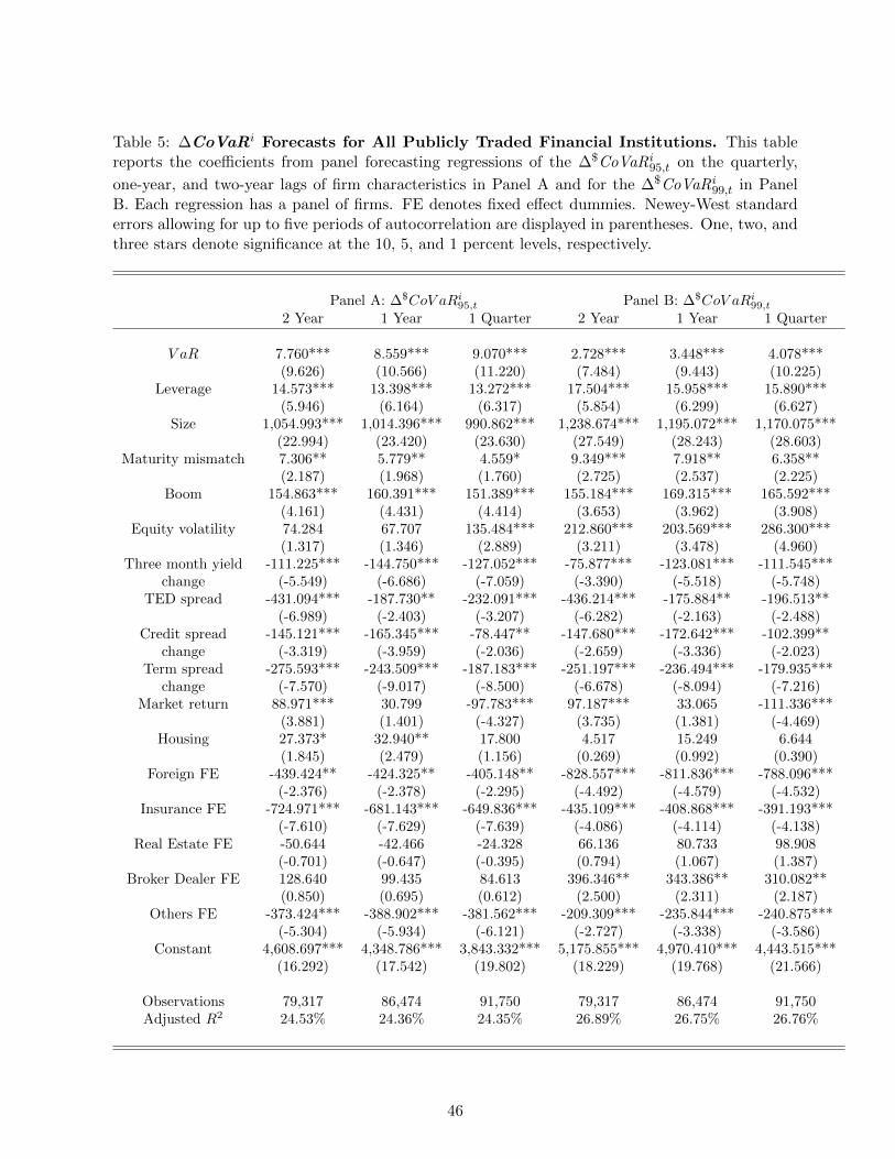
Table 5: ∆CoVaRi Forecasts for All Publicly Traded Financial Institutions. This tablereports the coefficients from panel forecasting regressions of the ∆$CoVaRi

95,t on the quarterly,

one-year, and two-year lags of firm characteristics in Panel A and for the ∆$CoVaRi99,t in Panel

B. Each regression has a panel of firms. FE denotes fixed effect dummies. Newey-West standarderrors allowing for up to five periods of autocorrelation are displayed in parentheses. One, two, andthree stars denote significance at the 10, 5, and 1 percent levels, respectively.

Panel A: ∆$CoV aRi95,t Panel B: ∆$CoV aRi

99,t

2 Year 1 Year 1 Quarter 2 Year 1 Year 1 Quarter

V aR 7.760*** 8.559*** 9.070*** 2.728*** 3.448*** 4.078***(9.626) (10.566) (11.220) (7.484) (9.443) (10.225)

Leverage 14.573*** 13.398*** 13.272*** 17.504*** 15.958*** 15.890***(5.946) (6.164) (6.317) (5.854) (6.299) (6.627)

Size 1,054.993*** 1,014.396*** 990.862*** 1,238.674*** 1,195.072*** 1,170.075***(22.994) (23.420) (23.630) (27.549) (28.243) (28.603)

Maturity mismatch 7.306** 5.779** 4.559* 9.349*** 7.918** 6.358**(2.187) (1.968) (1.760) (2.725) (2.537) (2.225)

Boom 154.863*** 160.391*** 151.389*** 155.184*** 169.315*** 165.592***(4.161) (4.431) (4.414) (3.653) (3.962) (3.908)

Equity volatility 74.284 67.707 135.484*** 212.860*** 203.569*** 286.300***(1.317) (1.346) (2.889) (3.211) (3.478) (4.960)

Three month yield -111.225*** -144.750*** -127.052*** -75.877*** -123.081*** -111.545***change (-5.549) (-6.686) (-7.059) (-3.390) (-5.518) (-5.748)

TED spread -431.094*** -187.730** -232.091*** -436.214*** -175.884** -196.513**(-6.989) (-2.403) (-3.207) (-6.282) (-2.163) (-2.488)

Credit spread -145.121*** -165.345*** -78.447** -147.680*** -172.642*** -102.399**change (-3.319) (-3.959) (-2.036) (-2.659) (-3.336) (-2.023)

Term spread -275.593*** -243.509*** -187.183*** -251.197*** -236.494*** -179.935***change (-7.570) (-9.017) (-8.500) (-6.678) (-8.094) (-7.216)

Market return 88.971*** 30.799 -97.783*** 97.187*** 33.065 -111.336***(3.881) (1.401) (-4.327) (3.735) (1.381) (-4.469)

Housing 27.373* 32.940** 17.800 4.517 15.249 6.644(1.845) (2.479) (1.156) (0.269) (0.992) (0.390)

Foreign FE -439.424** -424.325** -405.148** -828.557*** -811.836*** -788.096***(-2.376) (-2.378) (-2.295) (-4.492) (-4.579) (-4.532)

Insurance FE -724.971*** -681.143*** -649.836*** -435.109*** -408.868*** -391.193***(-7.610) (-7.629) (-7.639) (-4.086) (-4.114) (-4.138)

Real Estate FE -50.644 -42.466 -24.328 66.136 80.733 98.908(-0.701) (-0.647) (-0.395) (0.794) (1.067) (1.387)

Broker Dealer FE 128.640 99.435 84.613 396.346** 343.386** 310.082**(0.850) (0.695) (0.612) (2.500) (2.311) (2.187)

Others FE -373.424*** -388.902*** -381.562*** -209.309*** -235.844*** -240.875***(-5.304) (-5.934) (-6.121) (-2.727) (-3.338) (-3.586)

Constant 4,608.697*** 4,348.786*** 3,843.332*** 5,175.855*** 4,970.410*** 4,443.515***(16.292) (17.542) (19.802) (18.229) (19.768) (21.566)

Observations 79,317 86,474 91,750 79,317 86,474 91,750Adjusted R2 24.53% 24.36% 24.35% 26.89% 26.75% 26.76%

46

Table 6: ∆CoVaRi Forecasts For Bank Holding Companies. This table reports the coeffi-cients from panel predictive regressions of ∆CoVaRi

t on the quarterly, one year, and two year lagsof liability and firm characteristics in Panel A, and for asset and firm characteristics in Panel B.The methodologies for computing the risk measures VaRi

t and ∆CoVaRit are given in the captions

of Tables 2 and 3. The risk measures are caluclated for the 95% quantile. Newey-West standarderrors allowing for up to 5 periods of autocorrelation are displayed in patentheses. One, two, andthree stars denote significance at the 10, 5, and 1 percent levels, respectively.

Panel A: BHC Liability Variables Panel B: BHC Asset Variables

2 Year 1 Year 1 Quarter 2 Year 1 Year 1 Quarter

V aR 9.995*** 11.068*** 11.699*** 4.251** 6.402*** 7.715***

(4.774) (5.099) (5.310) (2.211) (3.305) (3.977)

Leverage 56.614*** 44.044*** 38.639*** 40.779*** 29.967*** 23.919***

(9.654) (9.683) (9.340) (6.476) (6.103) (5.532)

Size 1,457.875*** 1,394.324*** 1,360.318*** 1,203.344*** 1,141.656*** 1,107.145***

(13.539) (13.781) (13.850) (13.069) (13.352) (13.591)

Boom 88.923 108.619 90.283 124.161* 143.028** 123.243**

(1.238) (1.617) (1.560) (1.758) (2.179) (2.209)

Equity volatility 92.400 -55.501 48.969 292.221*** 90.937 165.272

(0.821) (-0.527) (0.436) (2.672) (0.887) (1.521)

Three month yield -541.105*** -512.923*** -442.339*** -357.807*** -343.193*** -278.257***

change (-6.815) (-6.442) (-7.344) (-5.567) (-5.145) (-5.585)

TED Spread -709.255*** -230.846 -448.387* -622.720*** -142.805 -369.578*

(-3.784) (-0.830) (-1.926) (-3.688) (-0.548) (-1.716)

Credit spread -338.997*** -268.226** -136.785 -208.571* -113.161 35.318

change (-2.860) (-2.082) (-1.132) (-1.879) (-0.935) (0.297)

Term spread -838.872*** -681.318*** -556.294*** -640.835*** -505.287*** -391.500***

change (-6.863) (-7.575) (-8.060) (-6.521) (-6.886) (-6.718)

Market return -16.289 -61.080 -205.718*** 25.380 -34.474 -188.620***

(-0.329) (-1.156) (-3.698) (0.541) (-0.706) (-3.601)

Housing 88.442*** 116.009*** 69.066** 64.023** 95.015*** 51.096*

(2.853) (4.091) (2.297) (2.236) (3.687) (1.795)

Core deposits -50.915*** -53.888*** -53.439***

(-8.005) (-8.217) (-8.244)

Non-interest deposits 51.610*** 46.680*** 43.844***

(3.840) (4.278) (4.519)

Time deposits -68.087*** -65.152*** -62.553***

(-8.347) (-8.123) (-8.064)

Demand deposits -13.782 -14.811 -16.195

(-0.929) (-1.254) (-1.511)

Total loans 9.419** 6.568* 3.811

(2.285) (1.792) (1.106)

Loan loss reserves -133.352 -131.401 -72.177

(-1.086) (-1.263) (-0.776)

Intanglible assets 48.721 43.285 41.082

(0.884) (0.874) (0.915)

Trading assets 576.060*** 565.476*** 549.158***

(5.332) (5.636) (6.088)

Constant 10,820.323*** 10,077.831*** 9,222.897*** 5,825.307*** 5,127.386*** 4,404.582***

(10.244) (10.388) (11.572) (7.899) (7.849) (8.573)

Observations 25,578 28,156 30,128 25,481 28,060 30,030

Adjusted R2 28.94% 28.17% 28.13% 36.29% 35.47% 35.41%

47

Table 7: ∆CoVaRi Forecasts For Bank Holding Companies. This table reports a regressionof the ∆CoVaR during the financial crisis of 2007-2009 on forward -∆CoVaR for the universe ofbank holding companies. The columns correspond to different forecasting horizons at differentdates. The first column is a two year forecast as of 2006Q4, the second column is a one yearforecast as of 2007Q4, the third column is a one month forecast as of 2008Q3, the fourth column isa one year forecast as of 2006Q4, and the last column is a one quarter forecast as of 2006Q4. One,two, and three stars denote significance at the 10, 5, and 1 percent levels, respectively.

Crisis ∆CoV aR

2008Q4 2008Q4 2008Q4 2007Q4 2007Q1

2Y Forward-∆CoV aR (2006Q4) 1.206***

1Y Forward-∆CoV aR (2007Q4) 0.664***

1Q Forward-∆CoV aR (2008Q3) 1.708***

1Y Forward-∆CoV aR (2006Q4) 0.848***

1Q Forward-∆CoV aR (2006Q4) 0.541***

Constant 13.08*** 18.51*** 2.409*** 4.505*** 2.528***

Observations 378 418 430 428 461

R2 36.6 % 17.8 % 78.9 % 49.6 % 55.5%

48

Table 8: ∆CoVaRi Forecasts using GARCH estimation. This table reports the coefficientsfrom panel forecasting regressions of the two estimation methods of ∆$CoVaRi

95,t on the quarterly,one-year, and two-year lag of firm characteristics. FE denotes fixed effect dummies. The GARCH -∆$CoVaRi

95,t is computed by estimating the covariance structure of a bivariate diagnonal VECHGARCH model. Newey-West standard errors allowing for up to five periods of autocorrelation aredisplayed in parentheses. One, two, and three stars denote significance at the 10, 5, and 1 percentlevels, respectively.

2 Year 1 Year 1 QuarterQuantile GARCH Quantile GARCH Quantile GARCH

V aR 10.655*** 22.126*** 10.462*** 22.290*** 10.760*** 22.953***(7.146) (6.446) (8.292) (6.762) (9.025) (7.725)

Size 2,171.414*** 3,650.023*** 2,088.345*** 3,495.286*** 2,044.432*** 3,432.149***(21.404) (16.656) (21.865) (16.792) (22.064) (17.000)

Maturity mismatch 22.292*** 40.001** 18.708** 30.449** 15.859** 28.336*(2.709) (2.207) (2.540) (1.975) (2.405) (1.898)

Boom 224.188*** 371.613*** 250.597*** 459.495*** 243.163*** 440.275***(3.060) (2.934) (3.417) (3.683) (3.448) (3.599)

Equity volatility 355.404*** 681.617*** 421.286*** 375.124 638.354*** 1,676.640***(2.772) (2.710) (3.493) (1.477) (5.375) (7.103)

Leverage 17.133*** 19.563* 17.383*** 18.788* 18.257*** 22.212**(2.655) (1.693) (2.975) (1.654) (3.249) (2.170)

Housing 16.228 82.042 3.684 -63.677 -29.998 -246.555***(0.460) (1.192) (0.116) (-1.018) (-0.784) (-3.338)

Three month yield -204.962*** -441.897*** -282.786*** -649.486*** -248.337*** -444.962***change (-4.476) (-5.124) (-5.584) (-6.105) (-5.854) (-6.116)TED spread -683.690*** -1,119.422*** -171.649 250.885 -249.432 -567.982*

(-4.966) (-4.386) (-0.937) (0.659) (-1.482) (-1.881)Credit spread -341.279*** -715.071*** -392.110*** -616.055*** -215.385** -45.730change (-3.295) (-3.572) (-3.959) (-3.461) (-2.319) (-0.239)Term spread -554.797*** -1,174.171*** -493.187*** -847.419*** -369.603*** -557.334***change (-6.508) (-6.821) (-7.809) (-7.419) (-7.159) (-6.241)Market return 97.262* 154.923 -36.331 -162.681 -329.304*** -490.855***

(1.875) (1.580) (-0.680) (-1.295) (-5.717) (-4.905)Foreign FE -600.936 -110.671 -608.110 -275.112 -580.752 -445.307

(-1.253) (-0.144) (-1.311) (-0.377) (-1.265) (-0.652)Insurance FE -1,550.564*** -3,500.083*** -1,421.556*** -3,254.618*** -1,339.724*** -3,054.498***

(-7.233) (-8.064) (-7.129) (-7.974) (-7.093) (-8.030)Real Estate FE 63.919 -34.037 156.418 68.235 223.824 234.309

(0.369) (-0.116) (0.982) (0.250) (1.483) (0.928)Broker Dealer FE 202.435 -775.272 253.854 -708.925 281.495 -664.763

(0.626) (-1.527) (0.820) (-1.442) (0.930) (-1.424)Others FE -682.642*** -1,535.849*** -656.751*** -1,546.880*** -626.059*** -1,418.808***

(-4.026) (-5.076) (-4.198) (-5.226) (-4.212) (-5.196)Constant 7,920.183*** 14,203.481*** 7,553.186*** 13,032.912*** 6,519.919*** 9,495.516***

(13.759) (11.613) (14.828) (12.660) (16.862) (13.664)

Observations 51,294 51,286 55,347 55,343 58,355 58,352Adjusted R2 27.10% 21.23% 26.94% 21.20% 27.00% 21.93%

49

Table 9: ∆CoVaRi Forecasts using alternative system returns variable. This table re-ports the coefficients from forecasting regressions of the two estimation methods of ∆$CoVaRi

95,t

on the quarterly, one-year, and two-year lag of firm characteristics. In the columns labeled Xsystem,∆$CoVaRi

95 is estimated using the regular system returns variable described in Section 3, whilein columns labeled Xsystem−i, ∆$CoVaRi

95 is estimated using a system return variable that doesnot include the firm for which ∆$CoVaRi

95 is being estimated. FE denotes fixed effect dummies.Newey−West standard errors allowing for five periods of autocorrelation are displayed in parenthe-ses. One, two, and three stars denote significance at the 10, 5, and 1 percent levels, respectively.

2 Year 1 Year 1 QuarterXsystem Xsystem−i Xsystem Xsystem−i Xsystem Xsystem−i

VaR 7.590*** 7.079*** 8.416*** 7.901*** 8.952*** 8.432***(9.375) (9.534) (10.326) (10.573) (10.974) (11.292)

Leverage 14.586*** 14.150*** 13.380*** 12.910*** 13.241*** 12.743***(5.988) (6.093) (6.178) (6.271) (6.316) (6.388)

Size 1,045.383*** 1,003.729*** 1,005.236*** 965.690*** 982.123*** 943.777***(22.846) (23.639) (23.263) (24.102) (23.461) (24.318)

Maturity mismatch 7.203** 6.349** 5.636* 4.970* 4.417* 3.900*(2.149) (2.138) (1.920) (1.902) (1.710) (1.684)

Boom 155.288*** 150.837*** 160.661*** 156.523*** 151.023*** 147.602***(4.203) (4.266) (4.470) (4.543) (4.445) (4.533)

Equity volatility 77.476 77.382 67.143 67.784 135.018*** 135.387***(1.389) (1.474) (1.337) (1.428) (2.897) (3.062)

Three month yield -110.309*** -104.495*** -143.529*** -137.320*** -125.988*** -120.507***change (-5.543) (-5.535) (-6.673) (-6.717) (-7.050) (-7.102)

TED spread -425.174*** -406.246*** -185.526** -172.485** -228.606*** -214.126***(-6.953) (-7.103) (-2.387) (-2.361) (-3.175) (-3.181)

Credit spread -144.973*** -137.867*** -160.705*** -154.783*** -75.179** -72.486**change (-3.391) (-3.416) (-3.929) (-3.987) (-1.984) (-2.006)

Term spread -274.462*** -262.126*** -242.640*** -231.757*** -185.570*** -176.715***change (-7.606) (-7.673) (-9.052) (-9.161) (-8.492) (-8.605)

Market return 88.292*** 84.502*** 29.547 27.823 -98.583*** -95.902***(3.848) (3.948) (1.349) (1.347) (-4.367) (-4.496)

Housing 27.667* 25.551* 33.085** 30.527** 18.043 15.607(1.860) (1.827) (2.491) (2.447) (1.168) (1.077)

Foreign FE -433.032** -420.804** -418.956** -407.989** -400.882** -391.199**(-2.336) (-2.366) (-2.343) (-2.378) (-2.266) (-2.304)

Insurance FE -712.369*** -656.614*** -669.666*** -617.652*** -639.305*** -589.511***(-7.496) (-7.395) (-7.516) (-7.428) (-7.527) (-7.439)

Real Estate FE -46.567 -37.370 -39.152 -31.187 -21.467 -14.662(-0.649) (-0.546) (-0.601) (-0.503) (-0.351) (-0.252)

Broker Dealer FE 113.499 139.780 84.969 110.399 69.907 94.869(0.757) (0.973) (0.599) (0.813) (0.510) (0.724)

Others FE -362.552*** -341.190*** -379.304*** -358.435*** -373.640*** -353.344***(-5.182) (-5.130) (-5.815) (-5.798) (-6.015) (-6.012)

Constant 4,573.181*** 4,393.954*** 4,310.730*** 4,146.631*** 3,805.569*** 3,658.264***(16.248) (16.599) (17.495) (17.884) (19.746) (20.250)

Observations 79,317 79,317 86,474 86,474 91,750 91,750Adjusted R-Squared 24.41% 25.13% 24.24% 24.96% 24.24% 24.96%

50

Table 10: Fraction of firms whose VaR estimates have correct conditional coverage.Per definition of the VaRt, losses at t should be less than the VaRt with probability 95% or 99%depending on the percentile. The table reports the fraction of firms that have correct conditionalcoverage at the 5% and 10% confidence levels based on Christoffersen’s (1998) likelihood ratio test.

Quantile GARCH5%-Level 10%-Level 5%-Level 10%-Level

95%− V aR 0.52 0.61 0.70 0.7899%− V aR 0.46 0.59 0.20 0.26

51