Coupler Design Issues from the Modular Ocean

Data Assimilation Project

Dr. Richard Loft

Computational Science Section

Scientific Computing Division

National Center for Atmospheric Research

Boulder, CO USA

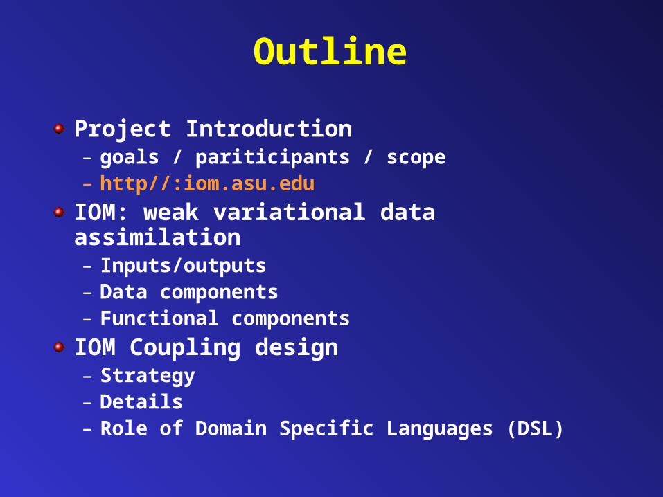
Outline

Project Introduction– goals / pariticipants / scope– http//:iom.asu.edu

IOM: weak variational data assimilation– Inputs/outputs– Data components– Functional components

IOM Coupling design – Strategy– Details – Role of Domain Specific Languages (DSL)

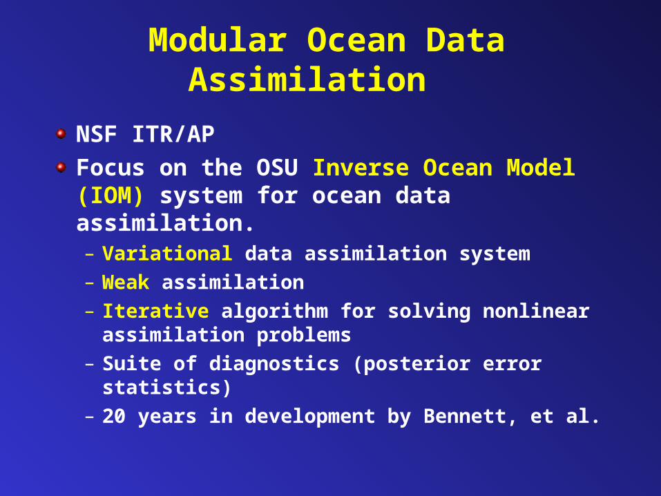
Modular Ocean Data Assimilation

NSF ITR/APFocus on the OSU Inverse Ocean Model (IOM) system for ocean data assimilation. – Variational data assimilation system– Weak assimilation– Iterative algorithm for solving nonlinear

assimilation problems– Suite of diagnostics (posterior error

statistics)– 20 years in development by Bennett, et al.

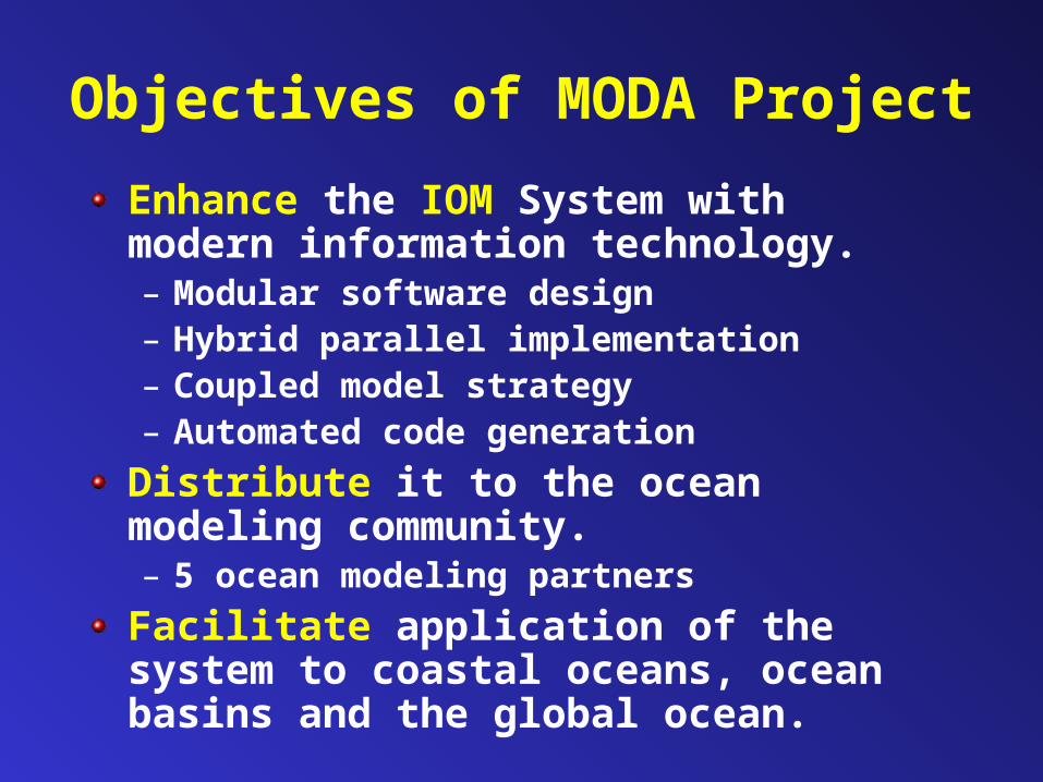
Objectives of MODA Project

Enhance the IOM System with modern information technology.– Modular software design– Hybrid parallel implementation– Coupled model strategy– Automated code generation

Distribute it to the ocean modeling community.– 5 ocean modeling partners

Facilitate application of the system to coastal oceans, ocean basins and the global ocean.

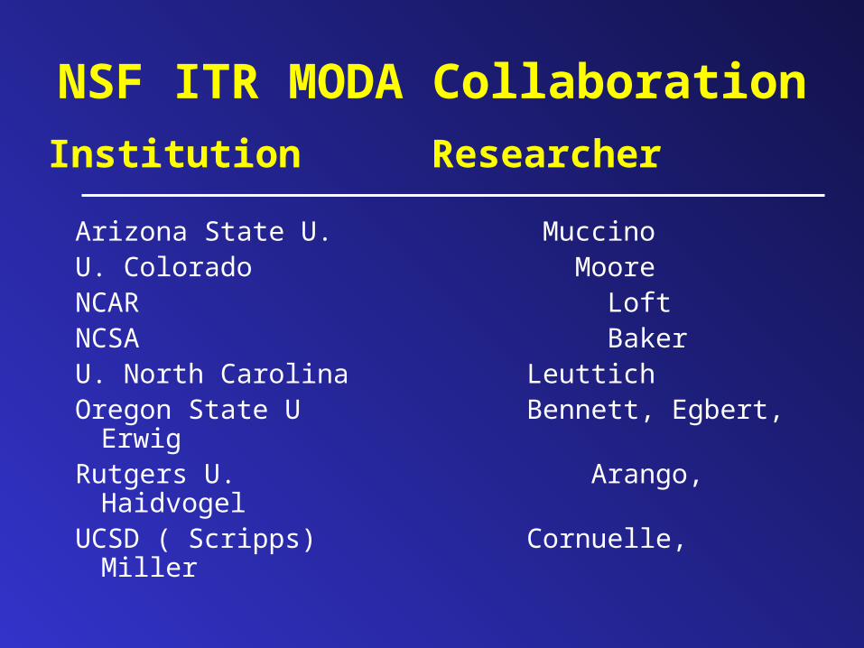
NSF ITR MODA Collaboration

Arizona State U. Muccino U. Colorado MooreNCAR LoftNCSA BakerU. North Carolina LeuttichOregon State U Bennett, Egbert,

ErwigRutgers U. Arango, HaidvogelUCSD ( Scripps) Cornuelle, Miller

Institution Researcher

IOM Team Members

IOM-PEZ Parallelism– PI: Rich Loft, NCAR– Component: parallel super and Infra-structure (hybrid F90 module framework)

Domain Specific Languages– PIs: Martin Erwig & Zhu Fu, OSU– Component: automated code generator

(Haskell)

Visualization– Pis: Polly Baker, NCSA/IU– Component: VisBenchTool Visualization

Software

Participating Model Teams

PEZ (Primitive Eq. Z-coordinate) model– Description: 3D, free-surface, z-

coordinate• Bryan-Cox

– Grid: spherical polar, “B” grid– Language: F90– Parallelism: SPMD, MPI

ROMS (Regional Ocean Model System)– Description: 3D, free-surface, S-

coordinate– Grid: Horizontal orthogonal curvilinear

coordinate, “C” grid– Language: F90– Parallelism: SPMD, OpenMP, MPI, SMS

Participating Model TeamsSEOM (Spectral Element Ocean Model) – PI: Dale Haidvogel, Rutgers– Description: 3D, free-surface, S-coordinate– Grid: h-p finite element, quadrilateral

element– Language: F90– Parallelism: SPMD, MPI

ADCIRC (Advanced Circulation) model– PIs: Julia Muccino, ASU; Rich Luettich, UNC– Description: 3D, free-surface, sigma-

coordinate– Grid: finite element, linear triangular

element Language: F90– Parallelism: SPMD, MPI

Participating Model TeamsOTIS (Internal Tides)– PI: Gary Egbert, OSU– Description: Laplace tidal equations plus

10 years of TOPEX/Poseidon– Description: Solid Earth mageto-tellurics

(magnetic field of earth’s crust)

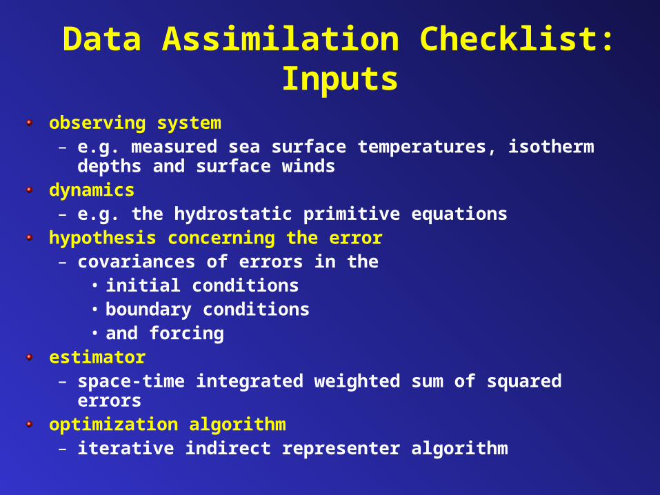
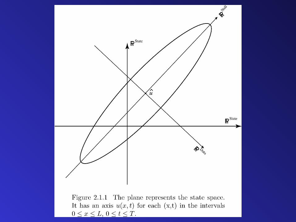
observing system– e.g. measured sea surface temperatures, isotherm

depths and surface windsdynamics – e.g. the hydrostatic primitive equations

hypothesis concerning the error– covariances of errors in the

• initial conditions• boundary conditions• and forcing

estimator – space-time integrated weighted sum of squared

errorsoptimization algorithm– iterative indirect representer algorithm

Data Assimilation Checklist: Inputs

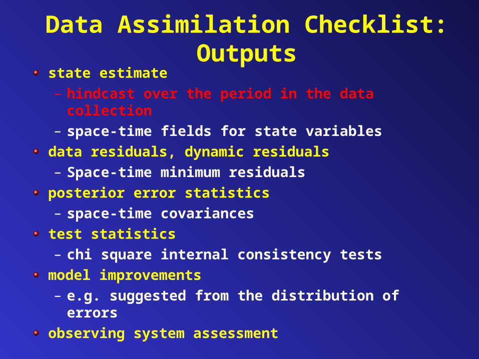
state estimate – hindcast over the period in the data

collection– space-time fields for state variables

data residuals, dynamic residuals– Space-time minimum residuals

posterior error statistics – space-time covariances

test statistics– chi square internal consistency tests

model improvements – e.g. suggested from the distribution of errors

observing system assessment

Data Assimilation Checklist: Outputs

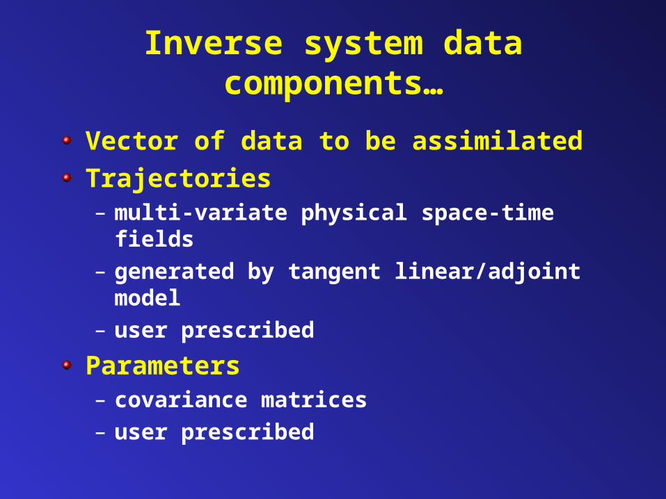
Inverse system data components…

Vector of data to be assimilatedTrajectories – multi-variate physical space-time fields– generated by tangent linear/adjoint

model– user prescribed

Parameters – covariance matrices – user prescribed

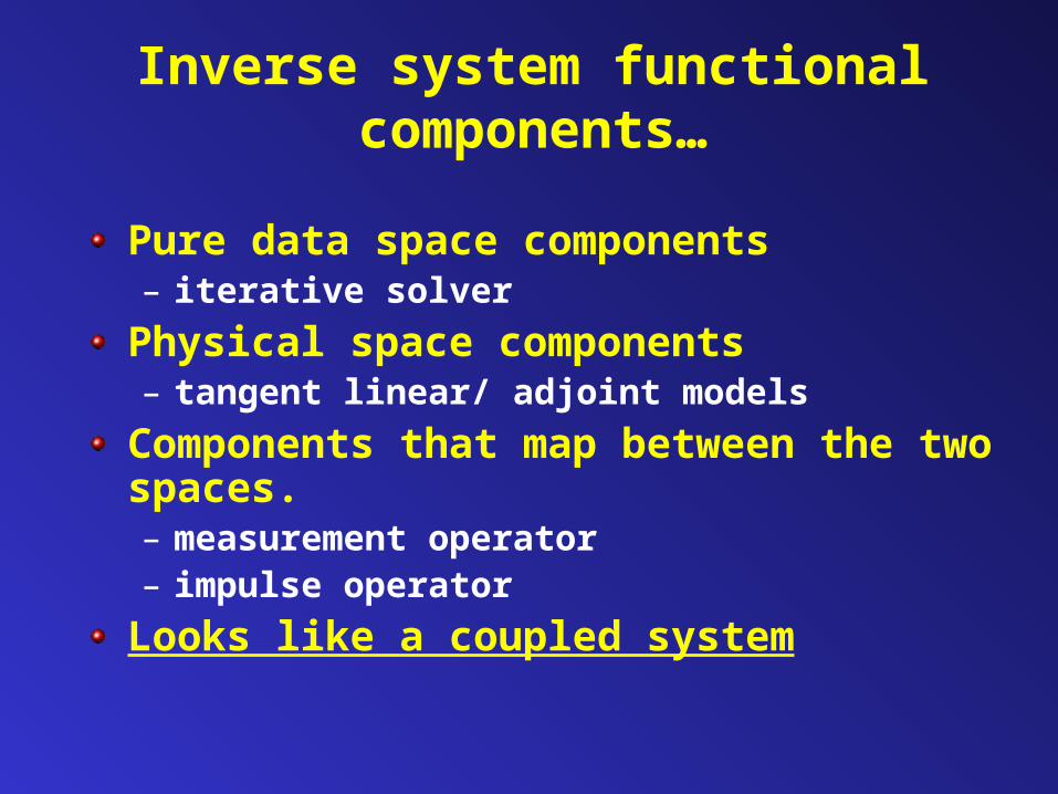
Inverse system functional components…

Pure data space components– iterative solver

Physical space components– tangent linear/ adjoint models

Components that map between the two spaces. – measurement operator– impulse operator

Looks like a coupled system

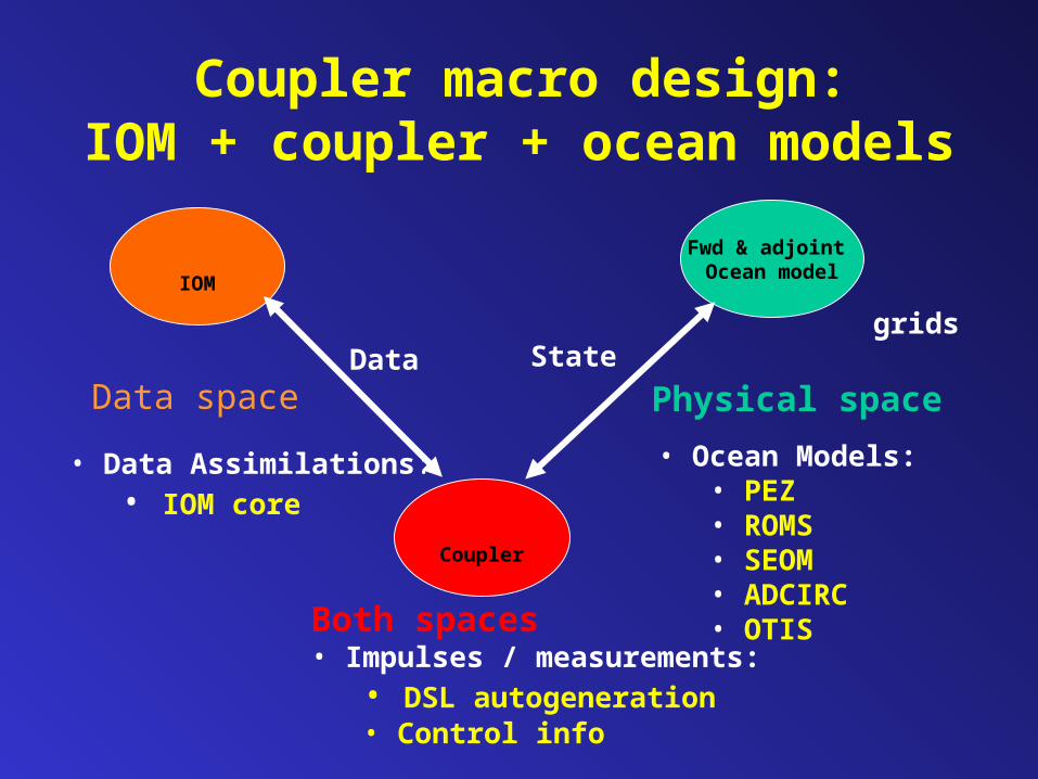
Coupler macro design: IOM + coupler + ocean models

Fwd & adjoint Ocean model

IOM

• Ocean Models:• PEZ • ROMS• SEOM • ADCIRC • OTIS

Physical spaceData space

• Data Assimilations:• IOM core

Data

Coupler

State

Both spaces• Impulses / measurements:

• DSL autogeneration• Control info

grids

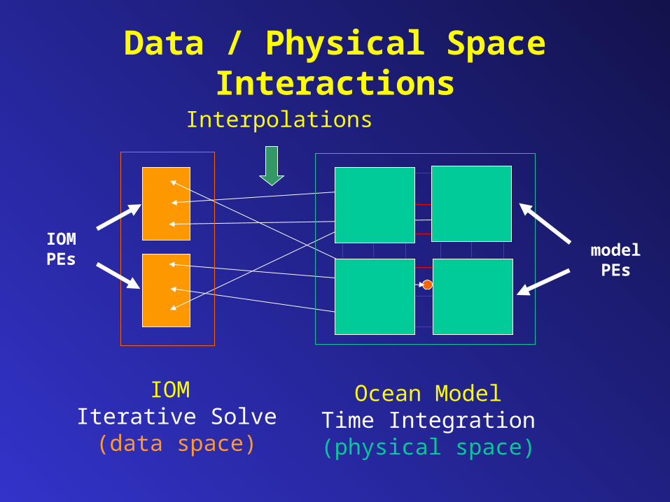
Data / Physical Space Interactions

Ocean ModelTime Integration(physical space)

IOM Iterative Solve(data space)

modelPEs

IOMPEs

Interpolations

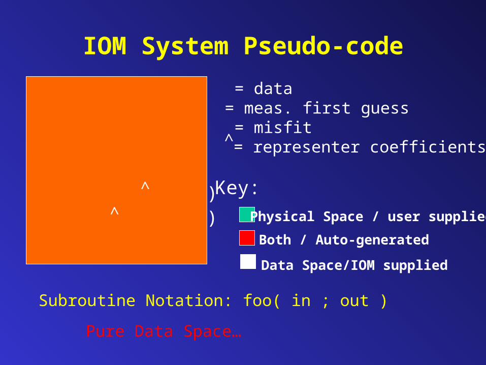
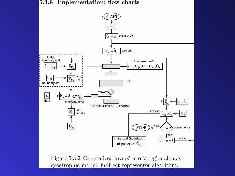
IOM System Pseudo-code

IOM(){ read d

first( ; uF) h = d - uF solve(h ; ) final( ; ) }

d = datauF = meas. first guessh = misfit = representer coefficients

Key:

Physical Space / user supplied

Both / Auto-generated

Data Space/IOM supplied

Subroutine Notation: foo( in ; out )

Pure Data Space…

^

^

^

IOM First Guess Code

first(;uF){ read F tanlin( F(x,t) ; UF(x,t) )

measure(UF(x,t) ; uF) }

F(x,t) = Initial / boundary / interior forcing

UF(x,t) = response to FuF = measured first guess

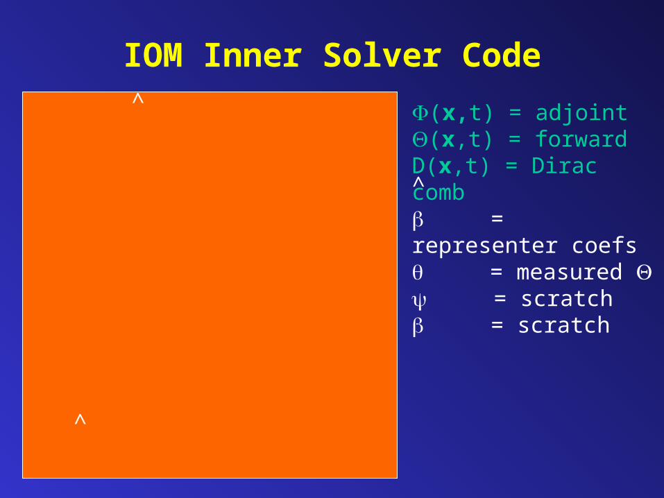
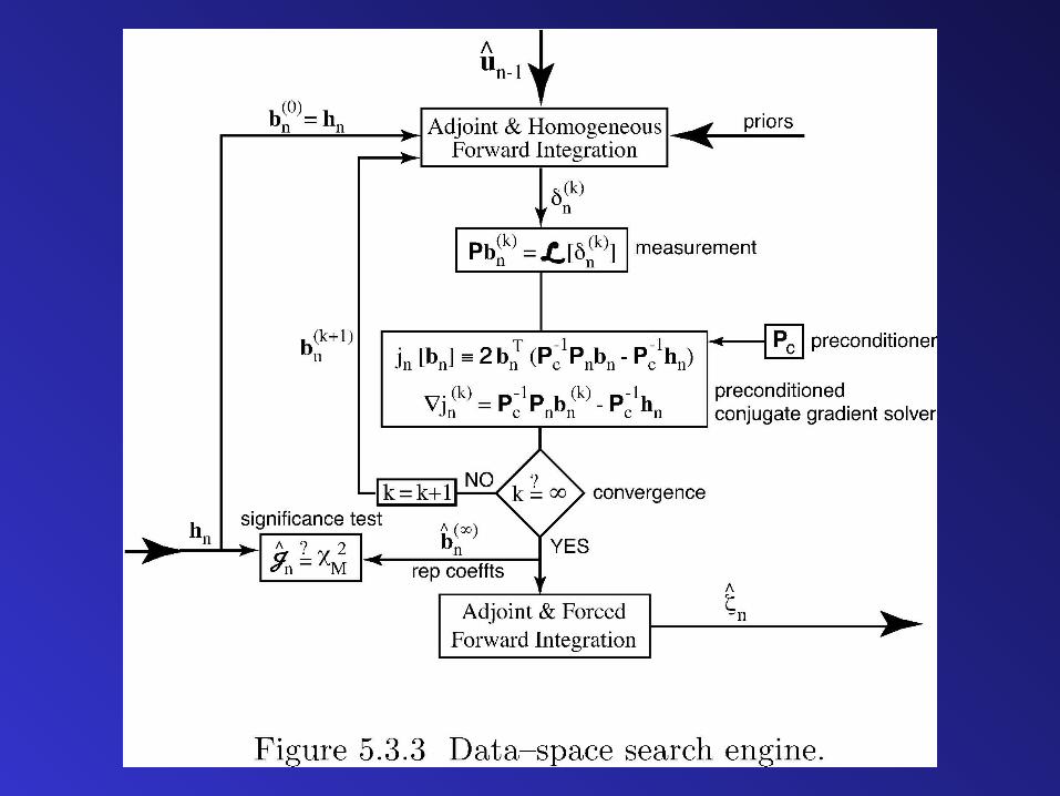
IOM Inner Solver Code

solve(h ; ){ = h

while ( ≠ ){ comb( ; D(x,t) )

adjoint( D(x,t) ; (x,t) ) convolve( (x,t) ; (x,t) )

tanlin( (x,t) ; (x,t) ) measure( (x,t) ; )

stabilize( , ; ) call precongrad( ; ) } = }

(x,t) = adjoint(x,t) = forwardD(x,t) = Dirac comb = representer coefs = measured = scratch = scratch

^

^

^

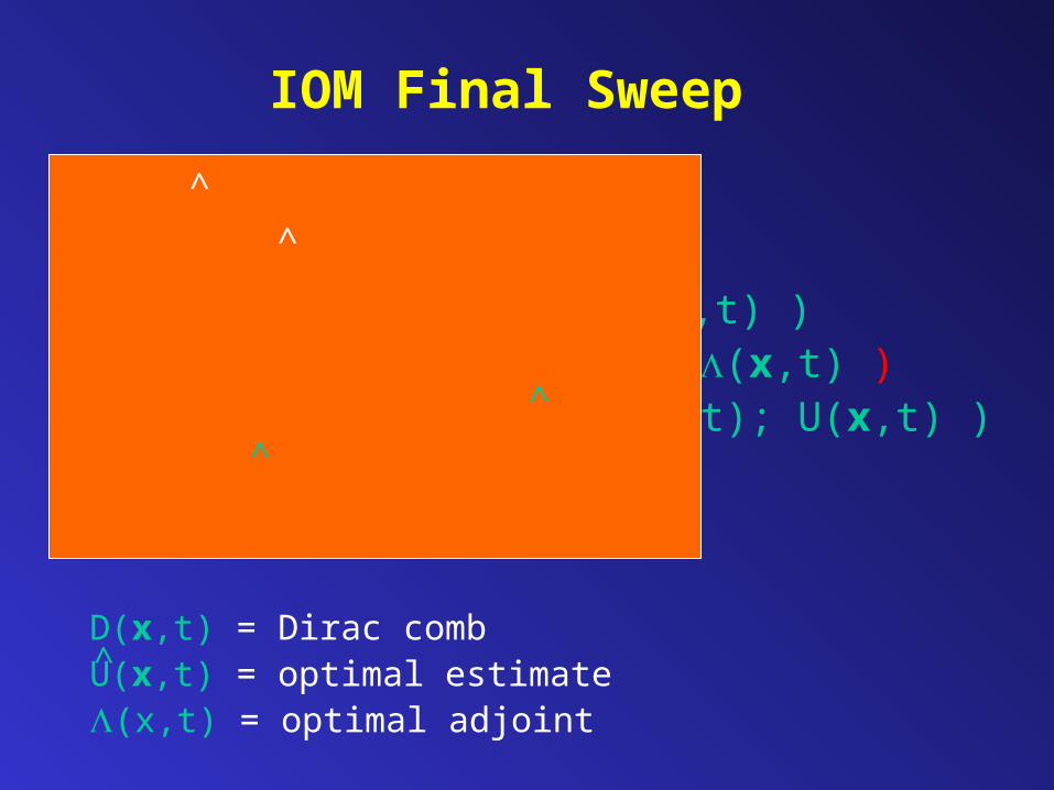
IOM Final Sweep

final( ; ){ comb( ; D(x,t) ) adjoint( D(x,t) ; (x,t) )

convolve( (x,t) ; (x,t) ) tanlin((x,t) + F(x,t); U(x,t) ) write U(x,t) }

D(x,t) = Dirac combU(x,t) = optimal estimate (x,t) = optimal adjoint

^

^

^

^

^

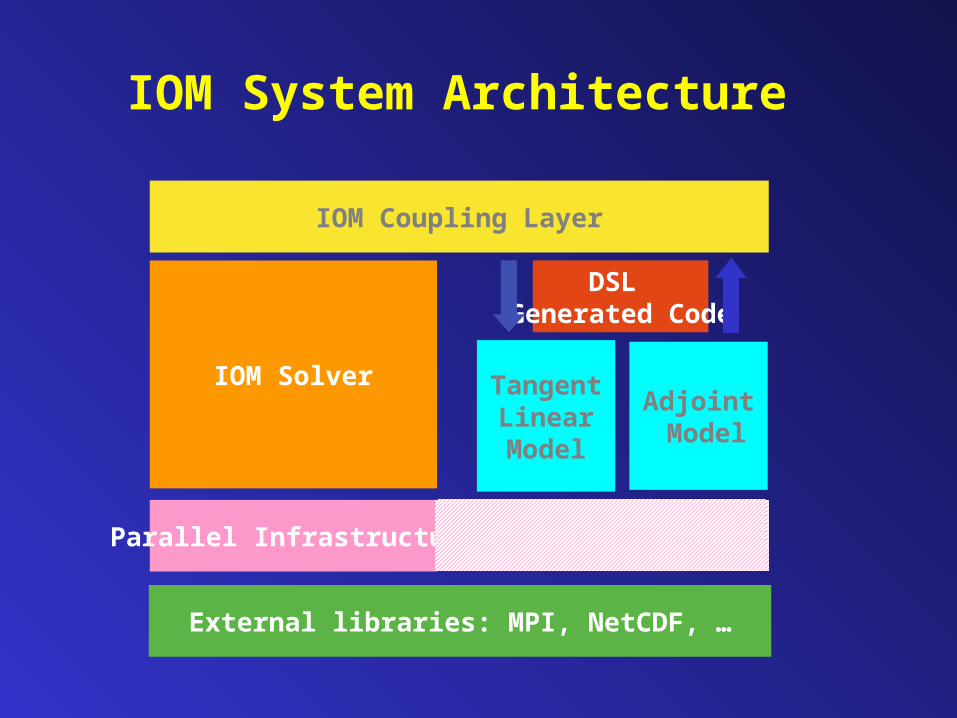
IOM System Architecture

Parallel Infrastructure

IOM Solver

IOM Coupling Layer

TangentLinearModel

DSL Generated Code

External libraries: MPI, NetCDF, …

Adjoint Model

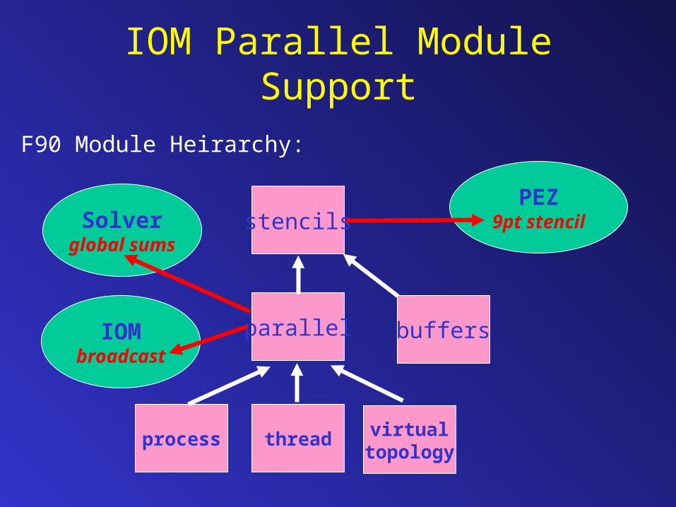
IOM Parallel Module Support

parallel

F90 Module Heirarchy:

process thread virtualtopology

PEZ9pt stencil

IOMbroadcast

stencils

buffers

Solverglobal sums

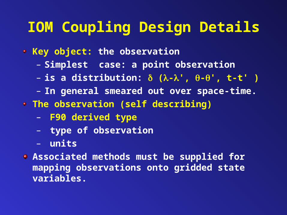
IOM Coupling Design Details

Key object: the observation – Simplest case: a point observation– is a distribution: (-', -', t-t' ) – In general smeared out over space-

time.The observation (self describing)– F90 derived type– type of observation– units

Associated methods must be supplied for mapping observations onto gridded state variables.

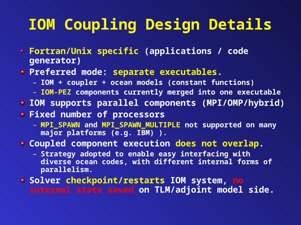
IOM Coupling Design Details

Fortran/Unix specific (applications / code generator)Preferred mode: separate executables.– IOM + coupler + ocean models (constant functions)– IOM-PEZ components currently merged into one executable

IOM supports parallel components (MPI/OMP/hybrid)Fixed number of processors – MPI_SPAWN and MPI_SPAWN_MULTIPLE not supported on many

major platforms (e.g. IBM) ).

Coupled component execution does not overlap.– Strategy adopted to enable easy interfacing with diverse

ocean codes, with different internal forms of parallelism.

Solver checkpoint/restarts IOM system, no internal state saved on TLM/adjoint model side.

Automatic Generation of Model-Specific IOM Tools

Martin Erwin and Zhe FuOregon State University

Idea:

Ocean modelers: • select simulation tools• provide parameters for their models• obtain a customized variational system

• Specify ocean modeling tools once• Identify model-dependent parameters• Generate Fortran programs from specification and values for parameters

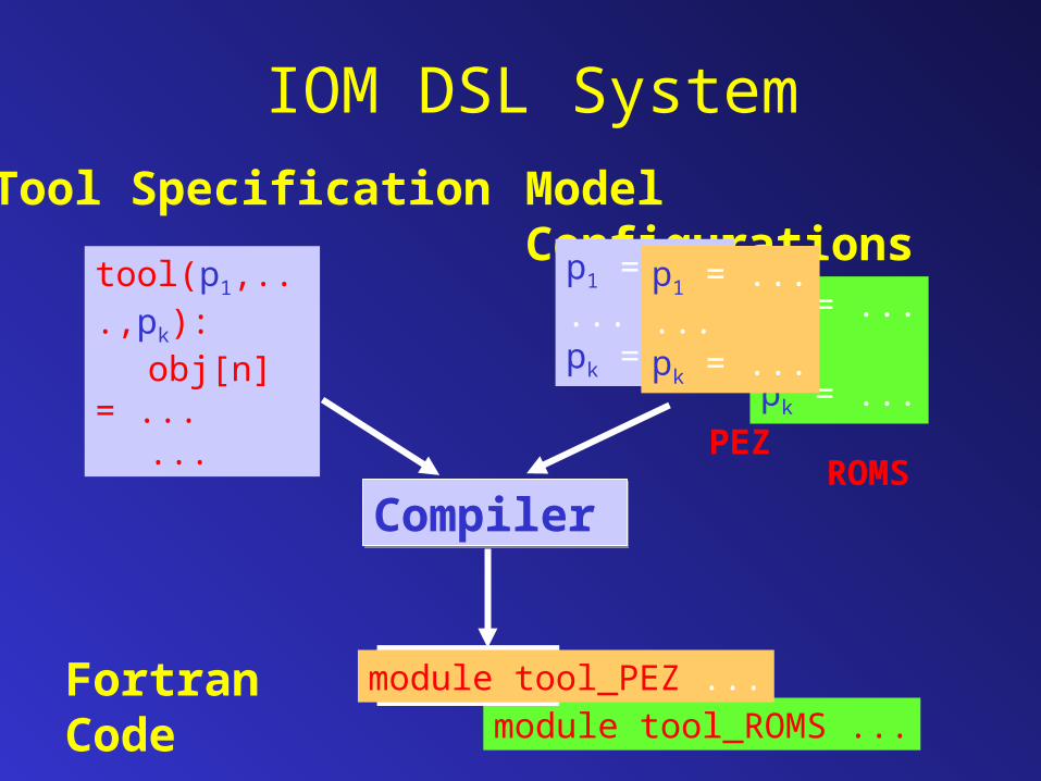
IOM DSL System

tool(p1,...,pk):obj[n] = ......

Tool Specification Model Configurations

p1 = ......pk = ...

Compiler Compiler

Fortran Code

p1 = ......pk = ...

module tool_ROMS ...

PEZROMS

p1 = ......pk = ...

module tool_PEZ ...

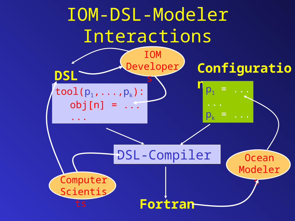
IOM-DSL-Modeler Interactions

tool(p1,...,pk):obj[n] = ......

DSL Configuration

p1 = ......pk = ...

DSL-Compiler DSL-Compiler

Fortran

ComputerScientists

OceanModelers

IOMDevelopers

Questions?