Copyright by Prince Nnamdi Azom 2013
266
Copyright by Prince Nnamdi Azom 2013
Transcript of Copyright by Prince Nnamdi Azom 2013

Copyright
by
Prince Nnamdi Azom
2013

The Dissertation Committee for Prince Nnamdi Azom certifies that this is the
approved version of the following dissertation:
IMPROVED MODELING OF THE STEAM-ASSISTED GRAVITY
DRAINAGE (SAGD) PROCESS
Committee:
Sanjay Srinivasan, Supervisor
Kishore Mohanty
Quoc Nguyen
Masa Prodanovic
Arjan Kamp

IMPROVED MODELING OF THE STEAM-ASSISTED GRAVITY
DRAINAGE (SAGD) PROCESS
by
Prince Nnamdi Azom, B.S.Ch.E.; M.S.E.
Dissertation
Presented to the Faculty of the Graduate School of
The University of Texas at Austin
in Partial Fulfillment
of the Requirements
for the Degree of
Doctor of Philosophy
The University of Texas at Austin
May 2013

Dedication
To the memory of my late mum…words can’t describe how much I would have wanted
you to see this day…you started this journey with me, but still hurts you didn’t wait to
see its end…I couldn’t have come this far without all the sacrifices you made…
To my wife, the unsung hero of this journey…without your patience and sacrifice, today
would have been impossible…at least, we can now have our honeymoon…
To my son, I guess you have one less excuse not to pursue a doctorate degree…of course
in any discipline of your choosing…I also hope you will one day read this dissertation
and be proud of what I’ve tried to achieve…

v
Acknowledgements
I would like to acknowledge my dad for his unending support and belief in me. As
a child, I couldn’t understand why you pushed me the way you did, yet today, it has made
all the difference.
To my siblings for such a beautiful and rewarding journey being your oldest
brother. I’ve watched all of you make unbelievable strides in your different fields and I
cannot be prouder. You have always outperformed my achievements and I know this will
also be one of them.
To my uncle, Ignatius Onedibe, your financial support couldn’t have come at a
better time during my undergraduate studies and I cannot thank you enough. Today is
also about your sacrifice of love and commitment you made to me more than a decade
ago.
To my mentor and friend, Obi Imemba, you not only made me realize and believe
I could pursue graduate studies in the US, but you have also redefined mentorship for me.
I hold that definition very close to my heart and have tried to live up to it as I mentor
others.
To all those who have impacted, in no small way, my improbable journey of
getting a doctorate degree – the Oyenuga’s, the Akinbode’s, the Olaniyan’s, the
Aderibigbe’s, the Akwukwegbu’s, my Aunt, Mrs. Edith Ekezie and so many more too
numerous to mention – I say a big thank you!

vi
To my professor, Dr. Sanjay Srinivasan, for his excellent tutorship and
supervision. I still remember the day I received the letter of funding from you back home
in Nigeria. You probably don’t know that if you hadn’t sent that letter, I probably would
not have attended UT. Your belief in me then and throughout my graduate studies has
been remarkable. I’ve learnt so much from you and have watched myself grow both
intellectually and emotionally since being your student. I recently looked at the first
presentation I gave under your supervision during the 2007 Heavy Oil Joint Industry
Project (JIP) at UT and my final PhD defense presentation, and couldn’t help but be
amazed at what time and a great supervisor can do with a young and naïve mind.
To members of my dissertation committee; Dr. Masa Prodanovic for the excellent
discussions we had on fascinating ideas such as implicitly determining the steam chamber
shape during SAGD and the Level Set Method, Dr. Arjan M. Kamp for your insights on
the effect of capillarity during SAGD and the life changing research experience I had
under your supervision during my 3 month stay at the Open and Experimental Centre for
Heavy Oil (CHLOE), Dr. Kishore Mohanty for helping me understand the limitations of
high temperature interfacial tension measurements and Dr. Quoc Nguyen for lending his
invaluable experience in the design and running of the experimental part of this
dissertation. Your comments during the final defense also helped produce a better
dissertation and graduate.
One of the advantages of attending a renowned University like the University of
Texas is that you get to learn and work with some of the best faculty in the world. Dr.
Larry Lake’s Enhanced Oil Recovery (EOR) class made me realize how much my
research on proxy modeling was desperately needed as recoverable reservoirs and
recovery processes become more complex for full blown numerical simulations to be
economical, Dr. Steven Bryant’s Advanced Transport Phenomena class taught me to

vii
never trust results from a numerical simulator and be the worst critic of my own work,
Dr. Gary Pope’s EOR class taught me to always question any published work and seek
out its underlying assumptions even if omitted by the author, Dr. Thomas Truskett’s
Advanced Fluid Flow and Heat Transfer class opened doors to analytically solving
complex partial differential equations (PDE’s) I didn’t even know existed at the time – a
skill that became invaluable in my research, Dr. Farzam Javadpour’s class on Advanced
Unconventional Reservoirs exposed me to the exciting world of Shale and Tight Gas
reservoirs for which we published an interesting paper together and I intend to pursue as
an additional research area post PhD. Of course there are other faculty I have not
mentioned, not for lack of impacting my education, but for space constraints. To all of
you, I say thank you for the great work that you do.
It is impossible to complete a dissertation that spanned experimental, simulation
and theoretical work without the help of several support staff. My SAGD experiment was
set up from scratch and such work would have been impossible to complete without the
help and expertise of Glen Baum and Jon Holder. Dr. Roger Terzian was excellent with
all my computer needs and support, our administrative assistant, Jin Lee, is probably the
reason we can even get any research done in our group and I was fortunate to be served
by two outstanding graduate coordinators – Cheryl Kruzie and more recently, Frankie
Hart.
Very few events apart from your education prepare you for success in the oil and
gas industry like an internship. At a time when it was almost impossible to get internship
positions due to the recession, a company with a brave and kind heart – Afren Resources,
USA – and its President, Shahid Ullah, took a huge gamble with me and few others and
offered us an opportunity I will always be thankful for. My several internships with
Afren, under the supervisions of Jim Ekstrand and George Zeito complimented

viii
beautifully my graduate education with the kind of practical experience most of my peers
seek but do not have.
To my fellow research group mates, both past and present; Kiomars
Eskandridalvand, Juliana Leung, Cesar Mantilla, Alvaro Barrera, Ankesh Anupam, Selin
Erzybek, Harpreet Singh, Darrin Madriz, Louis Forster, Tae Kim, John Littlepage,
Sayantan Bhowmik, Brandon Henke, Aviral Sharma, Pradeep Anand-Govind, Donovan
Kilmartin, Rami Abu-Rmaileh and the rest of the GAMMA team. Learning with and
from you has been so much fun.
I’ve also had the unbelievable luck of mentoring some of the brightest young
minds I’ve ever known during my doctoral studies through the Women-in-Engineering
Program (WEP) and the Petroleum and Geosystems Engineering (PGE) undergraduate
research internship program – Chris Yohe, Steven Fernandes, Travis Hampton,
Dhananjay Kumar, Omar El-Batouty, Katie Ruf and Kristina Baltazar. Each of these
great minds influenced my research in one way or the other and I will hold very fond
memories of what we achieved together, constantly being on the lookout for the
remarkable impact I know you will make in this world.
I would also like to appreciate several of my colleagues at the University of
Texas, both past and present for the wonderful learning experiences we had together;
Kelli Rankin, Abraham John, Olabode Ijasan, Lokendra Jain, Oluwagbenga Alabi, Amir
Reza, Ola Adepoju, Siyavash Motella, Femi Ogunyomi, Mardy Shirdel and so many
others I must have missed.

ix
Improved Modeling of the Steam-Assisted Gravity Drainage
(SAGD) Process
Prince Nnamdi Azom, Ph.D.
The University of Texas at Austin, 2013
Supervisor: Sanjay Srinivasan
The Steam-Assisted Gravity Drainage (SAGD) Process involves the injection of
steam through a horizontal well and the production of heavy oil through a lower
horizontal well. Several authors have tried to model this process using analytical, semi-
analytical and fully numerical means. In this dissertation, we improve the predictive
ability of previous models by accounting for the effect of anisotropy, the effect of heat
transfer on capillarity and the effect of water-in-oil (W/O) emulsion formation and
transport which serves to enhance heat transfer during SAGD.
We account for the effect of anisotropy during SAGD by performing elliptical
transformation of the resultant gravity head and resultant oil drainage vectors on to a
space described by the vertical and horizontal permeabilities. Our results, show that
unlike for the isotropic case, the effect of anisotropy is time dependent and there exists a
given time beyond which it ceases to have any effect on SAGD rates. This result will
impact well spacing design and optimization during SAGD.
Butler et al. (1981) derived their classical SAGD model by solving a 1-D heat
conservation equation for single phase flow. This model has excellent predictive
capability at experimental scales but performs poorly at field scales. By assuming a linear
saturation – temperature relationship, Sharma and Gates (2010b) developed a model that

x
accounts for multiphase flow ahead of the steam chamber interface. In this work, by
decomposing capillary pressure into its saturation and temperature components, we
coupled the mass and energy conservation equations and showed that the multi-scale,
multiphase flow phenomenon occurring during SAGD is the classical Marangoni (or
thermo-capillary) effect which can be characterized by the Marangoni number. At low
Marangoni numbers (typical of experimental scales) we get the Butler solution while at
high Marangoni numbers (typical of field scales), we approximate the Sharma and Gates
solution. The Marangoni flow concept was extended to the Expanding Solvent SAGD
(ES-SAGD) process and our results show that there exists a given Marangoni number
threshold below which the ES-SAGD process will not fare better than the SAGD process.
Experimental results presented in Sasaki et al. (2002) demonstrate the existence of
water-in-oil emulsions adjacent to the steam chamber wall during SAGD. In this work we
show that these emulsions enhanced heat transfer at the chamber wall and hence oil
recovery. We postulate that these W/O emulsions are principally hot water droplets that
carry convective heat energy. We perform calculations to show that their presence can
practically double the effective heat transfer coefficient across the steam chamber
interface which overcomes the effect of reduced oil rates due to the increased emulsified
phase viscosity. Our results also compared well with published experimental data.
The SAGD (and ES-SAGD) process is a short length-scaled process and hence,
short length-scaled phenomena (typically ignored in other EOR or conventional
processes) such as thermo-capillarity and in-situ emulsification should not be ignored in
predicting SAGD recoveries. This work will find unique application in predictive models
used as fast proxies for predicting SAGD recovery and for history matching purposes.

xi
Table of Contents
List of Tables ........................................................................................................xv
List of Figures .................................................................................................... xvii
Chapter 1: Introduction .......................................................................................1
1.1 Semi-Analytical vs. Fully Numerical Modeling....................................3
1.2 Motivation ................................................................................................4
1.2.1 The Effect of Anisotropy ............................................................5
1.2.2 The Effect of Capillarity (Multiphase Flow ahead of the Steam
Chamber) .....................................................................................5
1.2.3 The Effect of Flow and Transport of Water-in-Oil (W/O)
Emulsions .....................................................................................5
1.3 Contributions of this work .....................................................................6
Chapter 2: Review and Critique of Relevant Literature ................................10
2.1 Modeling the Steam-Assisted Gravity Drainage (SAGD) Process ...11
2.1.1 The Effect of Anisotropy ..........................................................17
2.1.2 The Effect of Capillarity (Multiphase Flow ahead of the Steam
Chamber) ...................................................................................21
2.1.3 The Effect of Flow and Transport of Water-in-Oil (W/O)
Emulsions ...................................................................................27
2.2 Modeling the Solvent-Aided Steam-Assisted Gravity Drainage (SA-
SAGD) Processes .........................................................................................30
2.2.1 The Steam and Gas Push (SAGP) ...........................................30
2.2.2 The Expanding Solvent Steam-Assisted Gravity Drainage
Process (ES-SAGD) ...................................................................31
Chapter 3: The Effect of Anisotropy .................................................................34
3.1 Model Development – Single Layer Reservoir ...................................35
3.1.1 Computing Oil Production Rate Accounting for Permeability
Anisotropy .................................................................................42

xii
3.1.2 Model Validation .......................................................................46
3.2 Model Development – Multiple Layered Reservoirs .........................49
3.2.1 Example Problem ......................................................................55
3.3 Results and Discussion ..........................................................................57
3.4 Summary and Significance of Work ...................................................71
Chapter 4: The Effect of Heat Transfer on Capillarity during SAGD ...........73
4.1 Model Development ..............................................................................74
4.1.1 Transport equations in a fixed frame......................................74
4.1.2 Transport equations in a moving reference frame ................78
4.1.3 Constitutive equations ..............................................................87
4.1.4 Dimensionless saturation profile .............................................89
4.1.5 A note on boundary conditions ................................................92
4.1.6 Oil rate .......................................................................................93
4.1.7 Dimensionless oil rate ...............................................................96
4.2 Model Validation ...................................................................................97
4.3 Results and Discussion ..........................................................................98
4.3.1 Sensitivity analysis ..................................................................111
4.4 Summary and Significance of Work .................................................118
Chapter 5: The Effect of Heat Transfer on Capillarity during ES-SAGD ..119
5.1 Model Development ............................................................................120
5.1.1 Transport equations in a fixed frame....................................121
5.1.2 Transport equations in a moving reference frame ..............122
5.1.3 Constitutive equations ............................................................128
5.1.4 Dimensionless saturation profile ...........................................132
5.1.5 Dimensionless oil rate .............................................................135
5.2 Results and Discussion ........................................................................138
5.2.1 Sensitivity analysis ..................................................................145

xiii
5.3 Summary and Significance of Work .................................................157
Chapter 6: The Effect of Emulsion Formation and Transport on Heat Transfer
during SAGD .............................................................................................159
6.1 Background .........................................................................................160
6.2 Mechanistic Model ..............................................................................162
6.2.1 Emulsion Generation ..............................................................166
6.2.2 Emulsion Propagation ............................................................167
6.2.3 Emulsion Coalescence .............................................................168
6.3 Modeling Procedure ............................................................................168
6.4 Experimental Model ...........................................................................170
6.5 Simulation Model ................................................................................170
6.6 Results and Discussion ........................................................................172
6.6.1 Sensitivity analysis ..................................................................187
6.7 Summary and Significance of Work .................................................194
Chapter 7: Conclusions and Recommendations ............................................196
7.1 Conclusions ..........................................................................................196
7.1.1 The Effect of Anisotropy ........................................................196
7.1.2 The Effect of Heat Transfer on Capillarity during SAGD .197
7.1.3 The Effect of Heat Transfer on Capillarity during ES-SAGD198
7.1.4 The Effect of Emulsion Formation and Transport during SAGD
...................................................................................................198
7.2 Recommendations for Future Work .................................................199
7.2.1 The Effect of Anisotropy ........................................................200
7.2.2 The Effect of Capillarity .........................................................200
7.2.3 The Effect of Emulsification ..................................................201

xiv
Appendix A .........................................................................................................202
Appendix B .........................................................................................................205
B.1 Coordinate Transform .......................................................................205
B.2 Mass Conservation Equation in a Moving Frame...........................207
Appendix C .........................................................................................................211
C.1 Experimental Modeling of the SAGD process .................................211
C.1.2 Experimental Procedure........................................................215
C.1.3 Experimental Results .............................................................215
Bibliography .......................................................................................................229
Vita ....................................................................................................................239
xv
List of Tables
Table 2.1: Showing the values of the modified Butler m parameter *m for the
different SAGD models...................................................................16
Table 3.1: Showing the values of reservoir parameters used in the anisotropic
model validation ..............................................................................48
Table 3.2: The v hk k ratio for each layer and the dimensionless thickness
distribution. The higher permeability anisotropy case is shown on
the left and the lower permeability anisotropy case is shown on the
right. .................................................................................................56
Table 3.3: Showing the multiphase flow factor for each v hk k ratio suitable for
comparing the semi-analytical model with numerical simulation
results ...............................................................................................62
Table 4.1: Showing the base case parameters used for SAGD ......................104
Table 4.2: Showing the history match parameters used to match Ito and Suzuki
(1999) data .....................................................................................109
Table 4.3: Showing the unknown parameters used to compute the thermo-
capillary numbers shown in Figs 4.12 & 4.13 of available
experimental and field data..........................................................111
Table 5.1: /g oiK - value parameters for Hexane from CMG (2011) .................129
Table 5.2: /g oiK - value parameters for Hexane obtained by regressing data from
Xu (1990) ........................................................................................129
Table 5.3: the HK - value parameters for Hexane obtained by fitting data in
Thimm (2006) ................................................................................131

xvi
Table 5.4: Base case reservoir and fluid parameters used for developing the ES-
SAGD results .................................................................................141
Table 6.1: Black-Oil Fluid Model with Emulsion Species ..............................165
Table 6.2: Properties of experimental sand pack (courtesy Sasaki et al. (2001a)
.........................................................................................................176
Table 6.3: Bitumen properties (courtesy Sasaki et al. (2001a) ......................177
Table 6.4: Bitumen viscosity (courtesy Sasaki et al. (2001a) .........................177
Table 6.5: Initial conditions and saturation endpoints (courtesy Sasaki et al.
(2001a) ............................................................................................177
Table 6.6: Showing the final model results and tuned parameters ...............178

xvii
List of Figures
Figure 1.1: Viscosity – Temperature relationship for some heavy oil reservoirs
(courtesy of Veil and Quinn 2008) ...................................................8
Figure 1.2: Viscosity – API – Temperature relationship for typical heavy oil
reservoirs (courtesy of Bennison 1998) ...........................................8
Figure 1.3: Schematic of a field scale application of the SAGD process with the
general physics displayed on the front view by the right (courtesy of
JAPEX). .............................................................................................9
Figure 2.1: Comparison plot showing the effect of anisotropy on SAGD oil
production rate ................................................................................18
Figure 2.2: Histogram of SAGD oil recoveries and their predictions using
different analytical models compared to the observed data .......25
Figure 3.1: Schematic of a typical SAGD steam chamber showing important
flow directions .................................................................................36
Figure 3.2: Schematic of an idealized SAGD steam chamber during horizontal
growth ..............................................................................................37
Figure 3.3: Plot of the % difference between the RGH and ROD models ....42
Figure 3.4: Schematic of an idealized SAGD steam chamber during horizontal
growth for a layered reservoir .......................................................49
Figure 3.5: Showing a finite difference based grid orientation during SAGD
horizontal growth with an effective permeability parallel to the
steam chamber wall similar to the vertical permeability ............61
Figure 3.6: Plot of dimensionless rate vs. dimensionless time for the RGH model
...........................................................................................................63

xviii
Figure 3.7: Plot of dimensionless steam chamber half width vs. dimensionless
time for the RGH model .................................................................63
Figure 3.8: Plot of ratio of anisotropic to isotropic dimensionless steam chamber
expansion vs. dimensionless time for the RGH model .................64
Figure 3.9: Plot of dimensionless rate vs. dimensionless time for the ROD model
...........................................................................................................64
Figure 3.10: Plot of dimensionless steam chamber half width vs. dimensionless
time for the ROD model .................................................................65
Figure 3.11: Plot of the ratio of anisotropic to isotropic dimensionless steam
chamber expansion vs. dimensionless time for the ROD model .65
Figure 3.12: Comparison plot of dimensionless rate vs. dimensionless time for the
RGH and ROD models ...................................................................66
Figure 3.13: Comparison plot of dimensionless steam chamber half width vs.
dimensionless time for the RGH and ROD model .......................66
Figure 3.14: Comparison plot of the ratio of anisotropic to isotropic
dimensionless steam chamber expansion vs. dimensionless time for
the ROD model ................................................................................67
Figure 3.15: Comparison plot of bitumen rate vs. time for the RGH, ROD and
numerical simulation models for constant multiphase flow
calibration factors ...........................................................................67
Figure 3.16: Comparison plot of bitumen rate vs. time for the RGH, ROD and
numerical simulation models for varying multiphase flow
calibration factors ...........................................................................68
Figure 3.17: Temperature profile from numerical simulation validation for
1v hk k ...........................................................................................68

xix
Figure 3.18: Water Saturation profile from numerical simulation validation for
1v hk k ...........................................................................................69
Figure 3.19: Water Saturation profile from numerical simulation validation for
0.3v hk k ........................................................................................69
Figure 3.20: Comparison plot of dimensionless rate vs. dimensionless time for the
layered and equivalent RGH and ROD models ...........................70
Figure 3.21: Comparison plot of dimensionless steam chamber half width vs.
dimensionless time for the layered and equivalent RGH and ROD
models...............................................................................................70
Figure 3.22: Comparison plot of the ratio of anisotropic to isotropic
dimensionless steam chamber expansion vs. dimensionless time for
the layered and equivalent RGH and ROD models .....................71
Figure 4.1: Schematic of the SAGD steam chamber showing important flow
directions and the steam chamber front velocity vector .............79
Figure 4.2: Plot of the dimensionless temperature – distance profile ahead of the
steam chamber interface for base case........................................104
Figure 4.3: Plot of the dimensionless water saturation – distance profile ahead
of the steam chamber interface for base case .............................105
Figure 4.4: Plot of the dimensionless water saturation – temperature profile
ahead of the steam chamber interface for base case ..................105
Figure 4.5: Plot of the dimensionless oil mobility – distance profile ahead of the
steam chamber interface for base case........................................106
Figure 4.6: Plot of the dimensionless oil rate vs. thermo-capillary number for
base case .........................................................................................106

xx
Figure 4.7: Plot of the oil saturation vs. dimensionless temperature for model
validation .......................................................................................107
Figure 4.8: Inversion plots for oil saturation vs. dimensionless temperature by a
modified Levenberg Maqardt technique ....................................107
Figure 4.9: Plot of the dimensionless water saturation – distance profile ahead
of the steam chamber interface for model validation ................108
Figure 4.10: Plot of the Leverett J function used for model validation and
sensitivities around it ....................................................................108
Figure 4.11: Plot of the derivative of the Leverett J function used for model
validation and sensitivities around it...........................................109
Figure 4.12: Column chart showing the distribution of dimensionless oil rate for
available experiment and field data ............................................110
Figure 4.13: Column chart showing the distribution of computed thermo-
capillary numbers for available experiment and field data ......110
Figure 4.14: Plot showing the correlation between the dimensionless oil rate and
computed thermo-capillary number for available experiment and
field data ........................................................................................111
Figure 4.15: Plot showing the sensitivity of the dimensionless oil rate vs. thermo-
capillary number to the Corey exponent a .................................114
Figure 4.16: Plot showing the sensitivity of the dimensionless oil rate vs. thermo-
capillary number to the Butler m parameter ..............................115
Figure 4.17: Plot showing the sensitivity of the dimensionless oil rate vs. thermo-
capillary number to the exponent of the interfacial tension –
temperature curve n .....................................................................115

xxi
Figure 4.18: Plot showing the sensitivity of the dimensionless oil rate vs. thermo-
capillary number to the Leverett J curve parameter .............116
Figure 4.19: Plot showing the sensitivity of the dimensionless oil rate vs. thermo-
capillary number to the fractional decrease in interfacial tension f
.........................................................................................................116
Figure 4.20: Plot showing the sensitivity of the dimensionless oil rate vs. thermo-
capillary number to the dimensionless initial mobile saturation wDS
.........................................................................................................117
Figure 4.21: Plot showing the sensitivity of the dimensionless water saturation
with distance from the steam chamber interface for thermo-
capillary number 1 0.01N to the Peclet number Pe ................117
Figure 5.1: Plot of the dimensionless temperature – distance profile ahead of the
steam chamber interface for the base case .................................142
Figure 5.2: Plot of the dimensionless water saturation – distance profile ahead
of the steam chamber interface for the base case .......................142
Figure 5.3: Plot of the dimensionless water saturation – temperature profile
ahead of the steam chamber interface for the base case ...........143
Figure 5.4: Plot of the dimensionless molar solvent concentration – distance
profile in the bitumen phase ahead of the steam chamber interface
for the base case ............................................................................143
Figure 5.5: Plot of the dimensionless molar solvent concentration – temperature
profile in the bitumen phase ahead of the steam chamber interface
for the base case ............................................................................144
Figure 5.6: Plot of the dimensionless oil mobility – distance profile ahead of the
steam chamber interface for the base case .................................144

xxii
Figure 5.7: Plot of the dimensionless oil rate vs. thermo-capillary number for
the base case...................................................................................145
Figure 5.8: Plot showing the sensitivity of the dimensionless oil rate vs. thermo-
capillary number to the Corey exponent a .................................150
Figure 5.9: Plot showing the sensitivity of the dimensionless oil rate vs. thermo-
capillary number to the Butler m parameter ..............................150
Figure 5.10: Plot showing the sensitivity of the dimensionless oil rate vs. thermo-
capillary number to the Leverett J curve parameter .............151
Figure 5.11: Plot showing the sensitivity of the dimensionless oil rate vs. thermo-
capillary number to the fractional decrease in interfacial tension f
.........................................................................................................151
Figure 5.12: Plot showing the sensitivity of the dimensionless oil rate vs. thermo-
capillary number to the dimensionless initial mobile water
saturation wDS ..............................................................................152
Figure 5.13: Plot showing the sensitivity of the dimensionless oil rate vs. thermo-
capillary number to the condensate Lewis number wLe ............152
Figure 5.14: Plot showing the sensitivity of the dimensionless oil rate vs. thermo-
capillary number to the dimensionless dispersion number *D ..153
Figure 5.15: Plot showing the sensitivity of the dimensionless oil rate vs. thermo-
capillary number to the viscosity ratio sol
s
................................153
Figure 5.16: Plot showing the sensitivity of the dimensionless oil rate vs. thermo-
capillary number to solvent concentration in the vapor phase iy 154

xxiii
Figure 5.17: Plot showing the sensitivity of the dimensionless oil rate vs. thermo-
capillary number to the dimensionless temperature difference *RT
.........................................................................................................154
Figure 5.18: Plot showing the sensitivity of the dimensionless oil rate vs. thermo-
capillary number to the dimensionless temperature difference *ST
.........................................................................................................155
Figure 5.19: Plot showing the water/oil equilibrium constant /w oiK from reservoir
to steam temperature ....................................................................155
Figure 5.20: Plot showing the sensitivity of the dimensionless oil rate vs. thermo-
capillary number to reservoir/injection pressure P ...................156
Figure 5.21: Plot showing the sensitivity of the dimensionless oil rate vs. thermo-
capillary number to the dimensionless initial water saturation wiDS
.........................................................................................................156
Figure 5.22: Plot showing the sensitivity of the dimensionless oil rate vs. thermo-
capillary number to the ratio of molar densities
msolmo
................157
Figure 6.1: Schematic representation of the steam chamber interface showing
the presence of W/O emulsions at the steam chamber interface
courtesy of Sasaki et al. (2002) .....................................................162
Figure 6.2: Schematic representation of the model for the water-in-oil
emulsification mechanism at the steam chamber interface ......169
Figure 6.3: 2-D simulation grid showing well placement ..............................171
Figure 6.4: Linear relative permeability curves for sand pack model (used by
Sasaki et al. 2001a) ........................................................................178

xxiv
Figure 6.5: Modeling permeability enhancement to oil on coalescence of
EMULSO (Kovscek, 2009) ...........................................................179
Figure 6.6: Comparison plot for cumulative oil recovery showing necessary
fitting values of permeability without emulsion modeling ........179
Figure 6.7: Comparison plot for cumulative oil recovery showing necessary
fitting values of porosity without emulsion modeling ................180
Figure 6.8: Comparison plot for cumulative oil recovery showing sensitivity to
joint porosity and permeability modeling using the Carman-Kozeny
relation without emulsion modeling ............................................180
Figure 6.9: Comparison plot for cumulative oil recovery showing necessary
fitting values for overall heat transfer coefficient and resin thermal
conductivity without emulsion modeling .................................181
Figure 6.10: Comparison plot for cumulative oil recovery showing the sensitivity
to the relative permeability exponent without emulsion modeling181
Figure 6.11: Comparison plot for cumulative oil recovery with the mechanistic
model for emulsion formation, propagation and coalescence ...182
Figure 6.12: Comparison plot for oil production rate with the mechanistic model
for emulsion formation, propagation and coalescence ..............182
Figure 6.13: Comparison plot for water-oil-ratio (WOR) with the mechanistic
model ..............................................................................................183
Figure 6.14: Steam chamber for experimental model at 550mint (courtesy
Sasaki et al., 2001a) © 1996 Society of Petroleum Engineers ...183
Figure 6.15: Steam chamber for mechanistic simulation model at 550 mint 184
Figure 6.16: Spatial localization of emulsion (EMULSO) droplets at 550 mint
.........................................................................................................184

xxv
Figure 6.17: Spatial localization of emulsion (EMULSO) droplets with dispersion
coefficient 20 cm minD at 550 mint ..........................................185
185
Figure 6.18: Half width of the steam chamber showing temperature (K) profiles
using COMSOLTM
Multiphysics .................................................185
Figure 6.19: Effective heat transfer coefficient (W/m-K) vs. volume % of
emulsion droplets for 0.05 mm droplets using COMSOLTM
Multiphysics...................................................................................186
Figure 6.20: Effective heat transfer coefficient vs. radius of emulsion droplets for
12.27% emulsion volume using COMSOLTM
Multiphysics......186
Figure 6.21: Sensitivity of cumulative oil recovery to the order of reaction. 189
Figure 6.22: Sensitivity of the water-oil ratio (WOR) to the order of reaction189
Figure 6.23: Sensitivity of cumulative oil production to the reaction rate constant
.........................................................................................................190
Figure 6.24: Sensitivity of the water-oil ratio to the reaction rate constant..190
Figure 6.25: Sensitivity of the cumulative oil recovery to the dispersion
coefficient of the emulsion droplets in oil ...................................191
Figure 6.26: Sensitivity of oil production rate to the dispersion coefficient of the
emulsion droplets in oil .................................................................191
Figure 6.27: Sensitivity of the water-oil ratio to the dispersion coefficient of the
emulsion droplets in oil .................................................................192
Figure 6.28: Sensitivity of the cumulative oil recovery to the enthalpy of
emulsification.................................................................................192
Figure 6.29: Sensitivity of the oil production rate to the enthalpy of
emulsification.................................................................................193

xxvi
Figure 6.30: Sensitivity of the water-oil ratio to the enthalpy of emulsification193
Figure B.1: Fixed and moving coordinate systems.........................................205
Figure C.1: Schematic of SAGD experimental model ....................................213
Figure C.2: Schematic of the square reservoir model used for the experiment
with some important dimensions .................................................214
Figure C.3: Temperature profile from SAGD experiment at time 2t minutes
.........................................................................................................217
Figure C.4: Temperature profile from SAGD experiment at time 12t minutes
.........................................................................................................218
Figure C.5: Temperature profile from SAGD experiment at time 22t minutes
.........................................................................................................219
Figure C.6: Temperature profile from SAGD experiment at time 32t minutes
.........................................................................................................220
Figure C.7: Temperature profile from SAGD experiment at time 42t minutes
.........................................................................................................221
Figure C.8: Temperature profile from SAGD experiment at time 52t minutes
.........................................................................................................222
Figure C.9: Temperature profile from SAGD experiment at time 62t minutes
.........................................................................................................223
Figure C.10:Temperature profile from SAGD experiment at time 72t minutes
.........................................................................................................224
Figure C.11:Temperature profile from SAGD experiment at time 82t minutes
.........................................................................................................225
Figure C.12:Temperature profile from SAGD experiment at time 92t minutes
.........................................................................................................226
xxvii
Figure C.13:Temperature profile from SAGD experiment at time 102t minutes
.........................................................................................................227
Figure C.14:Temperature profile from SAGD experiment at time 112t minutes
.........................................................................................................228

1
Chapter 1: Introduction
It is largely accepted that the immediate future of the oil industry lies in
unconventional resources, with heavy oil and bitumen as important classes of these
deposits. The world’s total resource of heavy oil in known accumulations is estimated by
the US Geological Survey (Meyer et al. 2007) to be 3.396 billion barrels of original oil in
place (OOIP) while that of bitumen is estimated to be 5,505 billion barrels OOIP. To put
this into context, these reserves are at least three (3) times the size of the world’s
conventional light crude reserves and the oil sands deposit in Canada is believed to be
larger than the oil reserves of Saudi Arabia. Even though the most talked about heavy oil
and bitumen deposits are the oil sands of Canada, there are several places in the world
where heavy oil and bitumen have been reported to exist (Meyer et al. 2007).
The classification of heavy crudes into heavy oil or bitumen is quite fuzzy and
there is currently no universally accepted criterion which is also made worse by the
existence of mini classifications like “extra-heavy oil” – used for bitumen that can flow at
reservoir conditions. A frequently used classification is one in which heavy oil has an
API gravity between 100API and 20
0API inclusive and a viscosity greater than 100cp
while bitumen has an API gravity less than 100API and a viscosity greater than 10,000cp
(Meyer et. al. 2007). Fig. 1.1 shows the viscosity – temperature relationship of some
known heavy oil reservoirs while Fig. 1.2 shows an example viscosity – API –
temperature correlation for typical heavy oils. For the purpose of this work, we will not
distinguish between heavy oil and bitumen, and from now on, will use the word
“bitumen” to describe both types of crudes unless otherwise stated.
There are several methods used to produce bitumen, one of the more popular
methods is Steam-Assisted Gravity Drainage, SAGD, and generally involves the injection

2
of steam into the upper of two horizontal wells, usually located 3 – 5m apart and the
production of the drained bitumen through the bottom well as shown in Fig. 1.3. The
injected steam forms a steam chamber above the well pair, and bitumen is produced
along the edges of the chamber to the producing well by the aid of gravity. Bitumen flow
and hence production is initiated and enhanced by the flow of heat from the steam zone
and through the condensate interface to the bitumen phase. The
condensate interface is a mixture of condensed steam and bitumen of low viscosity
(comparable in magnitude to the water at the interface temperature).
The SAGD process is a thermal enhanced oil recovery (EOR) technique whose
basic physics is relatively simple and involves the growth of a steam chamber and the
drainage of lower viscosity oil along the chamber wall by gravity. Hence, the taller the
steam chamber, the larger the oil drainage rate and this was first mathematically
described by Roger M. Butler and co-workers – who also invented the process – in their
classical drainage equation (Butler et al. 1981). However, like all EOR processes, the
basic physics is usually not enough and several other complex phenomena need to
described and coupled to either completely describe the process or improve its
predictability significantly. Some of these processes include, but not limited to
Permeability Anisotropy: Butler’s model assumes that the reservoir is both
homogenous and isotropic. This is far from the case for most real reservoirs and it
is unclear how anisotropy will affect SAGD rates since the steam chamber
interface will most times lie in-between the principal axis of anisotropy during a
typical SAGD process.
Capillarity: Butler’s model ignores capillary pressure and so does almost all
other analytical and numerical models for the SAGD process. The reasoning has
been that most bitumen reservoirs usually have high permeabilities and hence will

3
have small capillary pressures. However this reasoning is at best incomplete,
because capillary pressure is also a function of temperature i.e. both interfacial
tension and wettability are functions of temperature and thermal gradients in these
can induce additional fluid flow currently not accounted for in any SAGD model.
Emulsification: Just as emulsions are prone to form during chemical EOR due to
the reduction of interfacial tension by the action of surfactants, emulsions are also
prone to form during thermal EOR due to the reduction of interfacial tension with
an increase in temperature. Both water-in-oil and oil-in-water emulsions have
been reported in field scale recoveries but only water-in-oil emulsion formation
has been proved to occur in-situ during SAGD (Sasaki et al. 2002). How the
formation and transport of water-in-oil emulsions affects SAGD recovery is very
poorly understood.
The challenge is that with increasing complexity, analytical models like Butler’s model
no longer remain valid and a transition has to be made to semi-analytical or fully
numerical models.
1.1 Semi-Analytical vs. Fully Numerical Modeling
Since the earliest development of the SAGD process and its theory, several
authors have attempted to better understand the process and account for other complex
phenomena not included in the original Butler model. This has led to a plethora of models
used to describe the process, ranging from simple analytical models to complex semi-
analytical models. However, the inadequacies of these models together with the
requirement to support operational considerations such as spacing of wells, the amount of
steam injected etc. has led to the routine use of fully numerical models to predict its
4
recovery. The benefit of such numerical models is that they can be used to design field
implementations of the SAGD process, but the challenge rests in their inadequacy to
generate and test comprehensive theories that operate at different scales. This is a key
strength of analytical approaches. Also, the cost of running such simulations and the
accompanying numerical issues that affect the quality of the numerical solutions will
continue to make the search for analytical or semi-analytical solutions to complex
problems attractive. Another crucial reason to use semi-analytical models is that it is
easier to investigate new physics that affect the recovery performance whereas in fully
numerical models, this will require building a new simulator or significantly revamping
the data architectures of an existing one.
Previous semi-analytical models have either been too complex to justify their use
(Kamath et. al. 1993) or have included assumptions that are difficult to justify (Sharma
and Gates 2010). In this work, we use semi-analytical models to investigate some
physical characteristics of the SAGD process that have been inadequately studied in the
past. We also attempt to characterize the different heat transfer mechanisms that are
effective at the steam condensate-bitumen interface.
1.2 Motivation
Various researchers (Sasaki et al. 2001a), (Ito and Suzuki 1999), (Barillas et al.
2006) and (Donnelly 1998) have alluded to the difficulty in predicting the performance of
the SAGD process using numerical simulators. In some cases, they have reported an
under prediction of recovery while in others, overestimation of recovery have been
reported using traditional modeling and simulation approaches. This has motivated our
quest to include more physics in describing the SAGD process. In this work, we have

5
chosen to concentrate on the following three (3) aspects that affect SAGD recovery
performance.
1.2.1 The Effect of Anisotropy
SAGD is a gravity dominated process. In fact, in the original concept, there is no
other pressure gradient (Butler et al. 1981). This means that vertical permeability – hence
anisotropy – will have a very strong influence on SAGD recovery. As will be shown
later, it is very difficult to systematically vary v hk k in a finite difference numerical
simulator and get accurate results for the propagation of the steam chamber. This is
because of the stair-step behavior of fluid flow when the ratio is too low.
1.2.2 The Effect of Capillarity (Multiphase Flow ahead of the Steam Chamber)
Almost all current SAGD simulations ignore capillary behavior and they are not
included in any previous analytical or semi-analytical model. This is based on the
consensus that bitumen reservoirs have quite uniform pore geometries and high
permeabilities. However, capillary pressure is not only dependent on the radius of
curvature of fluid contacts in the porous medium but also on interfacial tension and
wettability, both of which can generally no longer be assumed constant especially for
strongly non-isothermal processes like SAGD.
1.2.3 The Effect of Flow and Transport of Water-in-Oil (W/O) Emulsions
As far back as the early days of the invention of the SAGD process, it has been
known that water-in-oil (W/O) emulsions are formed in-situ in the reservoir and produced
together with separate phases of condensate and bitumen (Chung and Butler 1989). It was

6
also assumed that since the emulsion phase will be more viscous than the pure bitumen
phase, that formation and transport of W/O emulsions will be detrimental to SAGD
recovery. However Sasaki et al. (2001a, 2001b, 2002) demonstrated the formation of
W/O emulsions at the walls of the steam chamber and hypothesized that this could
provide an additional heat transfer mechanism that enhanced recovery. In this work, we
will explain the reason for this supposed anomaly and the factors that influence it.
1.3 Contributions of this work
This work significantly enhances our understanding of the SAGD process as it
relates to the effects described in the motivation. The chapters are also divided
accordingly to reflect this.
In chapter 2, we give a thorough critique of available literature related to the
SAGD process and relevant to this work.
In chapter 3, we develop the semi-analytical model used to account for anisotropy
in both single layer and multilayered SAGD reservoirs. We show that conventional
averaging techniques will be inaccurate for the unique geometry of the SAGD process
and explain why we don’t get the typical constant maximum SAGD rate as predicted by
Butler’s theory for anisotropic reservoirs. In an attempt to validate the results using
numerical simulation, we will show why the results from finite difference based
numerical simulators should not be trusted for modeling the SAGD process in strongly
anisotropic reservoirs except in the impractical limit of infinitesimal grid sizes.
In chapter 4, we develop the semi-analytical model used to describe the effect of
capillarity on the SAGD process by accounting for non-isothermal multiphase flow ahead
of the steam chamber front using a physical effect called the Marangoni phenomena. We

7
also present an interesting discussion on why the Marangoni effect fundamentally
explains the controversial issue of the nature of convection during the SAGD process.
In chapter 5, we extend the modeling procedure in chapter 4 to account for non-
isothermal multiphase flow during the Expanding Solvent Steam-Assisted Gravity
Drainage Process (ES-SAGD), a variant of the SAGD process.
In chapter 6, we present a mechanistic model that explains the enhanced heat
transfer occurring at the steam chamber interface due to the formation of W/O emulsions.
We utilize the experimental data of (Sasaki et al. 2001b) for this purpose.
We conclude the dissertation in chapter 7 with a review of the key research
conclusions and future research issues.

8
Figure 1.1: Viscosity – Temperature relationship for some heavy oil reservoirs (courtesy
of Veil and Quinn 20081)
Figure 1.2: Viscosity – API – Temperature relationship for typical heavy oil reservoirs
(courtesy of Bennison 19982)
1 Veil and Quinn in their report cited personal communications with Dusseault M. B. as the source of this
figure

9
Figure 1.3: Schematic of a field scale application of the SAGD process with the general
physics displayed on the front view by the right (courtesy of JAPEX3).
2 This correlation is by Beggs and Robinson 3 Japan Exploration’s website page www.japex.co.jp/english/business/oversea/sadg.html

10
Chapter 2: Review and Critique of Relevant Literature
In this chapter, we will present a critique of past works on the SAGD process with
emphasis on its modeling. We will also pay particular attention to works that tried to
account for other complex phenomena apart from 1-D heat conduction, but restrict
ourselves to the central themes of this dissertation which are permeability anisotropy,
capillarity and water-in-oil (W/O) emulsion formation.
The SAGD process uses horizontal wells, hence permeability anisotropy will play
a strong role in recovery (Peaceman, 1993) yet it is unclear how it will do so since the
orientation of the fluid flow streamlines with respect to the principal axis of anisotropy
during a typical SAGD process will change with time. This alone will make any static
averaging technique i.e. arithmetic, harmonic etc. wrong. Also, numerical simulation
alone does very little to explain or explore this phenomena.
Ignoring capillary pressure effects during SAGD could be detrimental in our
understanding of the process as interfacial tension gradients – the so called Marangoni or
thermo-capillary effect (Nield, 1998), (Castor and Somerton, 1977) – could be of similar
order as that of thermal conduction. This is because for bitumen, the thermal conduction
length scale is small and only the bitumen in this length scale is produced during SAGD.
In fact, any short scale phenomena possibly occurring during SAGD should not be
ignored but rather investigated for the SAGD process. This paradigm makes the SAGD
process uniquely different from other thermal EOR processes or any other porous media
recovery process for that matter.
In-situ emulsification is another short scaled phenomena occurring during the
SAGD process since it comes about due to interfacial tension reduction at the steam
chamber interface. Emulsions have phase viscosities greater than their component phases,

11
hence, it can be argued that the formation of W/O emulsions can be detrimental to SAGD
recovery as some authors have stated (Chung and Butler, 1988), (Chung and Butler,
1989). However, these W/O emulsions are hot water droplets dispersed into the bitumen
phase and hence, should be principal carriers of convective heat energy thereby
improving recovery and not reducing it as has been shown to be the case by some authors
(Sasaki et al., 2001a), (Sasaki et al., 2001b), (Sasaki et al., 2002). Clearly, the increase in
both effective phase viscosity and heat transfer coefficient are competing physics and will
need to be further studied.
2.1 Modeling the Steam-Assisted Gravity Drainage (SAGD) Process
The Steam-Assisted Gravity Drainage (SAGD) process involves the injection of
steam and production of bitumen via pairs of horizontal wells that are usually separated 3
– 5 m apart, with the producer well at the bottom. The first attempt to model the SAGD
process was by Butler et al. (1981) where they assumed the only transport mechanism
was 1-D quasi-steady state heat conduction ahead of the steam chamber front and by
combining this with Darcy’s law gave the expression.
2 oo
os
S kg Hq
m
(2.1)
where
1
1 1
R
s
T
os
o oR RT
dTm v
v v T T
(2.2)
12
which is a parameter that relates how the viscosity-temperature curve changes from
reservoir to steam temperature and varies from about 3 – 5 for typical heavy oil and
bitumen reservoirs (Butler, 1991). The higher the value of m the lesser the viscosity-
temperature curve changes from reservoir to steam temperature.
Equation (A.1) states that the bitumen drainage rates is directly proportional to the
square root of porosity , mobile oil saturation oS , reservoir permeability k , acceleration
due to gravity g , thermal diffusivity and the thickness of the reservoir or bitumen
column H , and inversely proportional to the square root of the Butler parameter m and the
bitumen kinematic viscosity at steam temperature os . This means that a change in each of
these parameters will cause the same magnitude of change in the bitumen rates. This
result is quite interesting because it suggests a rather simple way of improving SAGD
rates – just increase any of the parameters in the numerator of (A.1) or decrease any of
the parameters in the denominator of (A.1). Since nature fixes ,g and H , we are left with
5 parameters as engineers to work with.
oS can be increased by delivering surfactants beyond the steam chamber
interface, but this will hardly double SAGD rates and might not be too beneficial in a
cumulative recovery sense since steam does a good job of reducing orS by the mechanism
of steam distillation (Hornbrook et al., 1991). Two important points to note here is that
surfactants tend to reduce interfacial tension which we will show in chapter 4 of this
dissertation diminishes recovery by the Marangoni or thermo-capillary effect, and
surfactants also tend to emulsify oil-water systems which will complicate any analysis on
SAGD recovery enhancement. In chapter 6, we will show that if water-in-oil emulsions
are formed at the steam chamber interface, SAGD recovery can be enhanced irrespective
of the increased bitumen phase viscosity (which by definition will be considerably less

13
than twice the bitumen component viscosity) because the thermal diffusivity can
practically double in value.
Permeability k can be enhanced through the geo-mechanical process of dilation
(Chalaturnyk and Li, 2004) or by hydraulic fracturing (Chen et al., 2008) while os and m
can be decreased by increasing steam temperature or co-injecting low viscosity solvent
with steam. However, care must be taken while increasing steam temperature because
there exists a temperature at a given pressure beyond which the latent heat of steam
begins to decrease.
It is most times desired to design laboratory experiments that will perform like a
given field scale recovery and for this, Butler et al. (1981) derived the dimensionless
group 2B useful for scaling laboratory experiments to field scale and given as
2
o s
mkgHB
S (2.3)
The value of 2B for both the experimental model and field scale reservoir must match for
both to be considered hydro-dynamically similar.
The factor m in equation (2.2) quantifies the effect of conductive heating on single
phase bitumen viscosity during SAGD. Equation (A.1) predicts that the oil rate is
constant and this equation only applies when the steam chamber has grown to the top of
the formation and is expanding horizontally till it confines the boundary of the reservoir.
This phase is called the horizontal or lateral growth phase in contrast to the vertical
growth phase (steam chamber development) and the depletion phase (Llaguno et al.,
2002). All parameters under the square root in equation (A.1) were assumed constant in

14
order to derive the analytical solution. Any attempt to make these parameters vary with
space and/or time, will at least require a semi-analytical model.
The first semi-analytical SAGD model was by Butler and Stephens (1981) where
they corrected equation (A.1) by replacing the 2 in (A.1) with 1.5 to account for the extra
head needed to move bitumen from the base of the reservoir to the producer well. It
required the approximation of drawing a tangent to the interface curves from the producer
well and was consequently called the Tangential Drainage (TANDRAIN) approximation.
We call this a semi-analytical model because it required an approximation (drawing of
the tangent) to an analytical expression. Butler (1991) also obtained another equation
which replaces the 2 in (A.1) with 1.3 and was called the Linear Drainage (LINDRAIN)
approximation.
Equation (A.1) was derived employing a quasi-steady state temperature
distribution assumption that allows a mass balance to be performed across a volume
element along the steam-bitumen interface. Relaxing this quasi-steady state assumption,
Butler (1985), developed a new approach to model the SAGD process using a heat
penetration variable. This gave rise to a set of equations with an ordinary differential
equation (ODE) that was solved for heat penetration, interface position and bitumen rates
given as
3 sinoD Dq B (2.4)
oDD
D
qU
L
(2.5)
33
2 1DD
D D
dB U
dt B
(2.6)

15
where oDq , D and DU are the dimensionless rates, heat penetration and interface velocity
respectively and 3B is a new dimensionless group given as
3
o s
kgHB
S m
(2.7)
which essentially performs the same role as 2B in the earlier theory. This new formulation
could account for boundary effects and hence formed the basis for Butler’s depletion
phase equations.
Reis (1992; 1993) argued that the quasi-steady state assumption for temperature
distribution used to derive (A.1) was incorrect due to its inadequacy for cases where the
local interface velocity is low, resulting in accumulation of mass at the interface. Reis
speculated that the interface velocity was not constant but changing in both magnitude
and direction typical of the SAGD process. He proposed a solution for the recovery rate
by assuming the local interface velocity to equal the maximum interface velocity at the
top of the chamber which he assumed to be constant. He then accounted for the effect of
lower velocities at other locations on the interface in an “average” sense by using an
empirical fitting constant. The results performed better than the Butler models for the
experimental data considered and his modified rate equation is given as
2o T
o
R os
S kg Hq
a m
(2.8)
where Ra is the Reis constant which he determined from his history match to be 0.4.

16
Akin (2005) presented a model that accounts for asphaltene deposition during
SAGD recovery by accounting for the increase in bitumen viscosity due to asphaltene
content in a Butler-type model similar to Reis’s development and it performed better than
the Butler and Reis model for the experimental data he used. Table 2.1 summarizes the
modifications to Butler’s equation for the flow rate in terms of the Butler m parameter to
account for the velocity and viscosity variations along the steam chamber interface.
Table 2.1: Showing the values of the modified Butler m parameter *m for the different
SAGD models
Model *m
Butler m
Tandrain 1.33m
Lindrain 1.54m
Reis 1.6m
Akin 4m
Nukhaev et al. (2006) corrected the Butler models by using shape factors that took
the geometry and approximation of chamber velocity into account. Their model
considered the case before steam break-through by accounting for the additional bitumen
rate due to the liquid head between the base of the steam chamber and the producer well.
Their model might be more accurate for situations where steam circulation was done
before initiating the SAGD process.
Najeh et al. (2009) presented a model that corrected the Butler models for
transient effects (i.e. the rate of propagation of the steam chamber) but however, their

17
approach will at best work for history matching purposes since there is currently no way
to explicitly model the interface velocity which is a critical and necessary parameter in
their formulation unlike the Butler models. Their results did better than the Butler models
only after fine tuning with the interface velocity dimensionless number.
2.1.1 The Effect of Anisotropy
While it is widely accepted that permeability anisotropy has a strong effect on
recovery processes that utilize a horizontal well such as SAGD (Peaceman, 1993), very
few studies have attempted to quantify anisotropy on SAGD process performance.
Najeh et al. (2009) used a geometric average of the vertical and horizontal
permeability for developing their semi-analytical SAGD model. No attempt was however
made to validate this assumption in their paper. It is our observation that the approximate
triangular shape of the steam chamber during the horizontal growth phase indicates that
the influence of the vertical permeability on bitumen rates should decrease just as the
influence of the horizontal permeability increases. The influence of permeability
anisotropy should therefore be time dependent.
Sharma et al. (2002) used a thermal simulator to perform a study of several
thermal recovery techniques including the SAGD process. They showed that anisotropy
influences SAGD bitumen rate, and their plots reveal a definite time component to this
phenomenon i.e., not only is the rate reduced for decreasing v hk k ratios, but the shape of
the plots though similar appear shifted in time as v hk k varies. One of these plots (Fig. 9
in their paper) is presented here for clarity in Fig. 2.1.

18
Figure 2.1: Comparison plot showing the effect of anisotropy on SAGD oil production
rate4
This result further suggests that any static averaging of the vertical and horizontal
permeabilities will be inadequate to model this phenomenon.
McLennan and Deutsch (2006) used accurately computed distribution of v hk k
ratios from mini-models to simulate steam chamber growth for the Surmount Lease in
Northern Alberta. Their results are quite interesting because Fig. 16 of their paper shows
a very irregular steam chamber shape as a result of heterogeneity and anisotropy. They
concluded that SAGD flow performance is quite sensitive to the spatial distribution of
permeability and to the contrast in vertical and horizontal permeability.
4 Courtesy of (Sharma et al., 2002), copyright, SPE.

19
Barillas et al. (2006) found that both heterogeneity and vertical permeability has a
major influence on SAGD oil recovery and optimal steam injection. However, their work
showed that cumulative oil recovery increases with a decrease in vertical permeability.
They commented on the non-intuitive nature of their results especially when compared
with the results in Sharma et al. (2002). They attributed the difference to steam
breakthrough and it is not clear if they used a steam trap in their simulations as that
would have significant impact on their conclusions. Their work reveals the difficulty of
comparing results from analytical and semi-analytical models with full numerical
simulations because events such as steam breakthrough that can entirely alter process
physics are not accounted for in analytical and semi-analytical models.
Sharma et al. (2002) also observed that when the vertical permeability was
increased beyond 200md for the given reservoir they modeled, it had no influence on
cumulative oil recovery. This suggests that there might be a specific combination of
reservoir and fluid properties for which the effect of anisotropy is unimportant to the
performance of the SAGD process. This conclusion is also supported by the work of
Kisman and Yeung (1995) who observed that lower v hk k ratios gave about 32% lower
production rates initially then gradually increased to about 8% of the isotropic base case
after about 8 years. This is not surprising from a purely geometric point of view because
as the steam chamber expands, depending on the lateral extent of the reservoir, there will
be a steam chamber angle for which the horizontal permeability influence on bitumen
rates dominates that of vertical permeability and this will also depend on the v hk k ratio.
We will prove this formally in a dimensionless framework in this dissertation.
Kamath et al. (1993) developed a 2D SAGD model based on Butler’s (1985)
modified SAGD model to account for factors such as heterogeneity, presence of shale
barriers and anisotropy. They found that the nature of heterogeneity has a complex effect

20
on the SAGD process as for any given heterogeneity index, it is better, in terms of
bitumen recovery, to have the horizontal producer in a higher permeability layer than in a
lower one. This is a consequence of using a transient formulation as the speed of
withdrawing bitumen by the producer can become a rate limiting step for the overall
SAGD process. This result can’t be obtained from a quasi-steady state model like the
Butler models. They also varied the Dykstra Parsons (DP) coefficient (Dykstra and
Parsons, 1950) and concluded that DP has a strong effect on recovery even though they
obtained a case (DP = 0.753) which had a higher recovery than for a purely homogenous
reservoir with same average permeability (DP = 0). The reason for this anomaly is that
their recovery prediction was responding to the multivariate distribution of the relative
location of the layers, the layer permeabilities and their thickness. They also presented
simulation results that showed the effect of anisotropy to be insignificant on recovery for
the reservoir and fluid properties studied. However, their well spacing of 200ft might
have been too small for a 900,000cp bitumen reservoir to see the full range of the
anisotropic rates as it varies from that due to mainly the vertical permeability to that due
to mainly the horizontal permeability. We will show in chapter 3 that the effect of
anisotropy is time dependent and there exists a dimensionless time after which its effect
ceases to affect SAGD rates. There might have also been numerical or other issues with
their simulation as their results show that close to the end of the simulation, the
cumulative oil recovery for 0.75v hk k is greater than that for the isotropic case.
Azad and Chalaturnyk (2010) and Azad (2012) were the first to present a
physically plausible analytic model for anisotropy used to account for oil saturation
evolution ahead of the steam chamber front due to geomechanics which they called the
Geomechanical Azad Butler (GAB) model. However, their intent was not to study the
effect of anisotropy but rather to quantify geomechanical effects during SAGD and hence

21
did not present any sensitivity to the v hk k ratio in their work. We will discuss their
anisotropy model further in this work and show that it is strictly not consistent with the
Butler type models.
What causes anisotropy is the presence of stochastic shales (Begg and Chang,
1985) laterally in the porous media (Deutsch, 2010) and these are shale barriers with
dimensions smaller than the size of a typical grid block. The v hk k ratio has been
calculated for these systems by considering the streamline path of a fluid particle as it
traverses a porous medium embedded with stochastic shales (Haldorsen and Lake, 1984).
If these shale barriers become larger than the size of a grid block, they lead to a
heterogeneous porous media which can also strongly affect the SAGD process (Yang and
Butler, 1992); (Chen et al., 2008); (Le Ravalec et al., 2009); (Shin and Choe, 2009).
Donnelly (1998) also claims that since the shale barriers are saturated with water, they
will be disintegrated under high temperatures due to the creation of internal stresses
during SAGD and this will cause anisotropy to be enhanced, making it a dynamic
(instead of the usual static) parameter. This claim is yet to be verified.
2.1.2 The Effect of Capillarity (Multiphase Flow ahead of the Steam Chamber)
Capillary pressure has been explicitly ignored from most analysis of the SAGD
process. In fact it is generally considered a secondary effect. Indirectly, it has been taken
into account mostly in numerical simulations of the SAGD process through relative
permeability curves. This also gives a sense of accounting for multiphase flow during the
SAGD process. We will distinguish between two kinds of multiphase flow during SAGD
– parallel to the steam chamber wall (condensate flow) and ahead of it (that controls the
transfer of heat to the bitumen). In the absence of other flow phenomena like the flow of

22
emulsions, SAGD fluid streamlines ahead of the steam chamber interface will be largely
parallel to the walls of the steam chamber, making multiphase flow parallel to the steam
chamber walls to be less important. Hence we will only consider capillarity ahead of the
steam chamber front (capillary imbibition).
As stated earlier, correcting the Butler models for multiphase flow effects started
with Butler himself in his second model (Butler and Stephens, 1981) and the LINDRAIN
(linear drainage) model (Butler, 1991). This was followed by models from Reis (1992;
1993) and Akin (2005). One characteristic of these multiphase flow corrections is the use
of an empirical constant to characterize its effect on the SAGD process. The inadequacy
of such an assumption is apparent as k in (A.1) has historically been used as a history
match parameter to capture the effective oil permeability (Butler, 1991).
More serious attempts to understand the phenomena of multiphase flow ahead of
the steam chamber front started – albeit unknowingly – with the work of Ito and Suzuki
(1999) where they used numerical simulation to conclude that the principal mechanism of
heat transfer during SAGD was by convection. It is still not clear how this is possible as
they stated their simulation runs had a pressure difference less than 40kPa between the
injector and the producer which is quite small compared to the specified maximum
bottomhole pressure (BHP) of 5000kPa to cause any appreciable convective fluid flux
ahead of the steam chamber interface. They also used small grid blocks to minimize
numerical dispersion which could cause a saturation gradient ahead of the steam chamber
interface. Their work was quite controversial, supported by (Farouq-Ali, 1997) and
disagreed with by (Edmunds, 1999) who argued that fluid streamlines during a typical
SAGD process should be nearly parallel to the steam chamber interface and hence should
have zero fluid flux orthogonal to it.

23
(Gotawala and Gates, 2008) argued that convection can occur ahead of the steam
chamber interface by the mechanism of steam fingering. They demonstrated that the
interface between the steam and the bitumen is generally hydro dynamically unstable.
However, the length scale of such instability is not expected to be considerable compared
to the reservoir thickness since gravity acts as a strong stabilizing force (Lake, 1996).
Sharma and Gates (2010b) inspired by the work of Ito and Suzuki (1999) modeled
multiphase flow effects explicitly by assuming a linear saturation-temperature profile
ahead of the steam chamber front with respect to temperature and included this in the
Butler-type model framework. Their model gave rise to a correction to the rate equation
that is a function of the Corey exponent of the oil relative permeability curve a , and the
Butler parameter m as in the following:
1 12
1o
o
os
m aS kg Hq
m m a
(2.9)
The Sharma and Gates model is flawed because it inherently assumes that thermal
diffusivity scales similarly as saturation diffusivity. As will be presented later, this cannot
be true because the principal mechanism of multiphase flow ahead of the steam chamber
front must be due to capillarity and not fluid convection (Edmunds, 1999, see also
response from Ito and counter-response).
Sharma and Gates (2011) also used this linear transport model to obtain an
effective thermal diffusivity ahead of the steam chamber interface due to convection and
was based on the work of Birrell (2003). Their model however gave a very poor fit to
Birrell’s data (see Fig. 10 of their paper) especially at the steam chamber interface. This
is because Birrell’s data has two parts to it – the thermal diffusivity at the steam chamber

24
interface, which will be mostly condensate saturated and the thermal diffusivity of the oil
sand ahead of the steam chamber interface, which will be mostly bitumen saturated.
Sharma and Gates (2011) model fit the bitumen saturated part – because this will just be
the thermal diffusivity of the oil sand – but did not fit the condensate saturated part.
McCormack (2001) observed a correlation between oil sand quality and recovery
as lower than theoretical average rates were obtained for average to poor sands. Since
factors that determine the quality of sands (for example grain size distribution) can be
linked to capillarity, this leads to the suggestion that capillary behavior can play an
important role during SAGD. Fig. 2.2 shows the histogram of available SAGD recoveries
and their predictions using several analytical models compared to the observed data. We
see that almost analytical models perform well at the experimental scale but perform
poorly at field scales. In contrast, the Sharma and Gates (S&G) model performs well at
field scales but poorly for the experimental data. This shows that multiphase flow during
SAGD is a multi-scale process and any method used to account for it should be accurate
across scales.
Most published works on the numerical simulation of the SAGD process ignore
capillary effects. The argument has been that the pore size distribution for most heavy oil
reservoirs is quite uniform (hence, negligible gradient in the Leverett J function) and
permeability high (hence, low capillary pressure). This assumption can only be adequate
for isothermal systems and fails considerable for non-isothermal systems such as SAGD.
This is because both interfacial tension and wettability can change with temperature in a
porous medium (Flock et al., 1986), (Bowman, 1967), (Serhat et al., 1999), (Torabzadey,
1984), (Castor and Somerton, 1977).

25
Figure 2.2: Histogram of SAGD oil recoveries and their predictions using different
analytical models compared to the observed data5
In fact, the gradient in interfacial tension and wettability due to temperature (and
solvent concentration in the case of injecting steam with solvent) can be greater than the
gradient in the Leverett J function (Leverett, 1941) due to non-uniform pore size
distributions. This is because at high water saturations, the Leverett J function has an
almost zero gradient while interfacial tension curves are fairly linear with temperature
(Bowman, 1967). Also, the capillary transport mechanism will change the saturation of
the wetting phase which in turn will create a gradient in the Leverett J function. These
three gradients (interfacial tension, wettability and saturation) sum up to give the total
capillary gradient with respect to temperature which will significantly impact the
transport characteristics during SAGD and can explain several discrepancies between
experiment and field scale recoveries. Several authors have termed this “multiphase flow
5 Courtesy of Sharma and Gates (2010b)
0
100
200
300
400
SA
GD
Oil
Ra
te (
m3
/da
y)
-p
er
we
ll p
air
Histogram of SAGD Oil Recoveries
Butler
Lindrain
Reis
S&G
Observed

26
effects” and have tried to quantify it using fudge factors and other simplifying
assumptions as stated earlier. In this work, we will attempt to present a cohesive theory to
explain and quantify this phenomenon based on the classical Marangoni or thermo-
capillary effect.
If thermo-capillarity is to play a role during SAGD, it must do so via a
mechanism, and its effect can only be important near the steam chamber interface. The
concept of capillary imbibition as a transport mechanism during SAGD has been reported
by several authors (Butler et al., 1994). Nasr et al. (2000) argued there must be coupled
flow going on at the steam chamber interface, and this coupled flow is countercurrent in
nature. Even though they did not give a mechanism for such coupled flow, their results
suggests such a mechanism can be countercurrent capillary imbibition with condensate
imbibing into the bitumen phase. Al-Bahlani and Babadagli (2009) mentioned water
imbibition as a flow mechanism during the SAGD process and Aherne and Maini (2008)
gave proof that water can move horizontally through an oil sand with the Dover project
where water was consciously injected into the reservoir without it being produced
concurrently. The challenge however, is to model this physics in a realistic framework.
Some authors have rightly questioned the ability of current commercial simulators to
model this effect (Nasr et al., 2000), and it is also our conclusion that current simulators
cannot adequately model this effect, and may only be able to do so via very complicated
indirect means. To give validity to these indirect methods will require a calibration or
history match. However, such model calibration will be non-unique and no explicit
conclusions regarding the occurrence or absence of such capillary mechanisms may be
possible.

27
2.1.3 The Effect of Flow and Transport of Water-in-Oil (W/O) Emulsions
The in-situ formation and transport of emulsions in porous media is not a new
phenomenon (Raghavan and Marsden., 1971a) and both oil-in-water (O/W) and water-in-
oil (W/O) emulsions are known to form depending on the state of the porous media.
Mehdizadeh (2005) suggests only the formation of O/W emulsions during SAGD in their
discussion of adequate flowmeters for the SAGD process while Arendo et al. (2005)
suggest both O/W and W/O emulsions form during SAGD and flowmeters should be
designed to handle both types of emulsions. Dalmazzone et al., (2010) stated they
received W/O emulsions from a heavy oil field in describing their de-emulsification
process while Sanyi et al. (2004) stated that only O/W emulsions always form during
SAGD. Noik et al. (2005) and Beetge (2005) went a step further to state that in addition
to W/O and O/W emulsions, other complex emulsion systems like water-in-oil-in-water
(W/O/W) and oil-in-water-in-oil (O/W/O) emulsions also do form during SAGD. Bosch
et al. (2004) argued only for the formation of O/W emulsions by stating that the high
temperatures and small density difference between bitumen and water at typical SAGD
operating conditions helps stabilize O/W emulsions. Georgie and Smith (2012) paper
suggests that W/O emulsions do form downhole during SAGD but can “invert” to O/W
emulsions during transport to surface facilities.
These field scale observations suggests the possibility of forming both types of
emulsions at some point during bitumen production, but it is not clear if both emulsions
are formed in-situ in the reservoir during SAGD. Also, they suggest that the quality of
injected steam and initial water saturation of the reservoir play significant roles in
deciding which of W/O or O/W emulsions are formed during a given SAGD operation.
This is because it is thermodynamically unfavorable for W/O emulsions to exist at high

28
water cuts characteristic of high initial water saturation reservoirs or low quality steam
injection processes. The reverse is also true for O/W emulsions.
Some experimental work has been done to study emulsion characteristics during
SAGD and it is worth noting that only the in-situ formation of W/O emulsions has been
reported experimentally. This shouldn’t discount the possibility of the in-situ formation
of O/W emulsions during SAGD because most field scale recoveries will be
characterized by lower steam quality and higher water cut than experimental scale
recoveries. This might explain why only W/O emulsions have been reported at
experimental scales.
The study of the flow and transport of water-in-oil (W/O) emulsions during
SAGD started with the work of Chung and Butler (1988) where they showed that
injecting steam from the top of the reservoir minimizes the formation of W/O emulsions
unlike the typical SAGD process of injecting steam just a few meters above the
production well. This result is quite interesting as it indicates that the mechanism of the
formation of W/O emulsions might be shear induced.
Chung and Butler (1988) also stated that oil recovery in the well will be reduced
because the emulsified phase will have a higher viscosity than the bitumen phase.
However, such analysis generally fails to take into account the complex mechanism of
fluid flow and heat transfer at the steam/bitumen interface. Water-in-oil (W/O) emulsions
are non-equilibrium, thermodynamically unstable phases (Sasaki et al., 2002), and differ
in this regard from the thermodynamically stable micro emulsions of chemical flooding
EOR. The presence of such emulsion was seen clearly for the first time in the work of
Sasaki et al. (2002) where they used an optical fiber scope to visualize the flow of the
W/O emulsion droplets and showed that it was impossible to match the experimental data
without accounting for their in-situ flow characteristics (Sasaki et al., 2001b); (Sasaki et

29
al., 2001a). We speculate in this work that such emulsions are formed at the
steam/bitumen interface due to shear induced instability (Raghavan and Marsden, 1971b)
and subsequently, the emulsion droplets are transported into the bitumen phase by
dispersion.
Chung and Butler (1989) extended their initial model to study the effect of initial
water saturation, steam quality, reservoir grain size and injection pressure. They found
that the lower the initial water saturation, the greater the degree of emulsification which
they explained on thermodynamic grounds to be the consequence of having a connected
water film in the reservoir. They also concluded that steam quality, reservoir grain size
and injection pressure do not significantly affect the emulsification process. It is however
important to note that the steam conditions they used was superheated to about 10 – 150C
above saturated steam, clearly creating conditions favorable for the formation of W/O
emulsions and hence their conclusions.
Cuthiell et al. (1995) studied W/O emulsification behavior in heavy oils and
determined that there exists a threshold point for emulsification which is characterized by
the capillary number cN given by
oc
ow
uN
(2.10)
and this value is about 10-3
to 10-4
which is easily attained for heavy oils. It is important
to note that their work did not consider non-isothermal systems like SAGD, and it is easy
to see from (2.10) that even for typical values at the steam chamber interface, cN will be
in the order of 10-5
to 10-6
which should not give rise to emulsification based on Cuthiell
et al.’s theory. This also suggests that in-situ emulsification during SAGD might be
occurring at a small, but finite distance away from the interface where oil viscosities are

30
larger, or a different mechanism is needed to explain W/O emulsification for non-
isothermal bitumen recovery processes.
Modeling this process of in-situ emulsification is quite challenging, because the
physics of emulsion formation and transport in porous media is not yet fully understood.
Current knowledge describes the process as induced by the difference in viscosity of two
adjacent liquid phases (Raghavan and Marsden, 1971b); (Raghavan, 1982); (Chuoke et
al., 1959).
2.2 Modeling the Solvent-Aided Steam-Assisted Gravity Drainage (SA-
SAGD) Processes
Solvent-Aided Steam-Assisted Gravity Drainage (SA-SAGD) processes were
developed to mitigate some of the limitations of the traditional SAGD process. These
limitations include high heat loss to the overburden and low thermal efficiencies. There
are several classifications of this modification of the SAGD process (Mohammadzadeh et
al., 2010) but we will classify the SA-SAGD process in this work by the intended
purpose of the aiding solvent. Based on this, only two commercially successful types of
the SA-SAGD process currently exists.
2.2.1 The Steam and Gas Push (SAGP)
This involves the co-injection of non-condensable gases (C1 – C2) with steam so
as to minimize heat losses to the overburden. It generally gives slightly lower drainage
rates (Butler, 1999) but conserves heat significantly. This is an extremely complicated
process from a modeling point of view because of the existence of 3-phase flow
(gas/oil/condensate) beyond the edge of the steam chamber unlike the SAGD process

31
where only oil/condensate flow occurs ahead of the steam chamber. The three phase
region exists because the non-condensable gas generally tends to diffuse appreciably
beyond the steam chamber edge. This can be seen clearly from the numerical simulations
of Al-Murayri et al. (2011) and very few models have been presented to analyze this
process from an analytical point of view.
To adequately model this process will not only require 3-phase relative
permeability curves but also gas/oil or gas/water capillary pressure curves in addition to
the oil/water curves. This difficulty can easily be seen in the work of Sharma et al. (2012)
where they accounted for the diffusion of the non-condensable gas and its partitioning
into the bitumen phase but had to assume linear oil saturation-temperature profiles and
linear gas saturation-distance profiles in their model. A model that incorporates the full
suite of capillary pressure models would have avoided such an assumption and yielded a
more accurate rate equation.
2.2.2 The Expanding Solvent Steam-Assisted Gravity Drainage Process (ES-SAGD)
This involves the co-injection of condensable gases (C3 – C8) with steam to
provide additional viscosity reduction of bitumen, thereby requiring less steam for the
same drainage rates which makes the ES-SAGD process more thermally efficient than the
traditional SAGD process. The ES-SAGD process is a blend of the Vapor Extraction
(VAPEX) process developed by Butler and Mokrys (1991) and the SAGD process. It was
initially conceived by Nasr et al. (2003) and has been shown to be quite successful in
recent pilot studies (Gupta and Gittins, 2006). Most of the modeling work done on the
ES-SAGD process have used numerical simulators (Ananth Govind et al., 2008) and very
few analytical models exist.

32
Sharma and Gates (2010a) noted the cross-dependencies of the solvent diffusion
coefficient and the bitumen phase viscosity and accounted for them in their steam-solvent
coupled model but did not present equations for enhanced bitumen rates due to solvent
dilution. Fig. 7 and Fig. 10 of their paper reveal that they could have assumed the
diffusion coefficient to be constant without adversely affecting the prediction of bitumen
rates. They also did not account for multiphase flow ahead of the steam chamber
interface in this work.
Rabiei Faradonbeh et al. (2012) coupled the quasi-steady state energy equation
with the transient component mass balance equation using the Heat Integral Method
(HIM) to develop a semi-analytical ES-SAGD model. Their model was however, not
fully dimensionless and this limited the generality of their conclusions. From their plots,
it also seems that they could have obtained similar results if they completely worked in a
quasi-steady state space i.e. using the snapshot of the mass transfer process at a particular
instant in time. This is because the length scale of mass transfer is so small compared to
that of heat transfer for its transient to have any significant impact on such a coupled
solution. They also did not account for multi-phase flow effects in their model.
Gupta and Gittins (2012) combined the SAGD and VAPEX equations in a quasi-
steady state framework to derive their semi-analytical ES-SAGD (which they call the
solvent-aided process (SAP)) model. Their model was quite unique in its simplicity and
showed the need to define a diffuse solvent layer ahead of the steam chamber to
accurately capture ES-SAGD physics. They also did not account for multi-phase flow
effects in their model.
To summarize, we have explored the current state of knowledge with respect to
modeling the SAGD and ES-SAGD processes and have identified three (3) effects –
anisotropy, capillarity and emulsification – that are currently weakly understood and

33
loosely accounted for, if at all, in current SAGD models. In chapter 3, we will extend the
Butler models to account for anisotropy during SAGD and show that it is a time
dependent phenomenon which depending on the scale of the well spacing, its effect
might be masked just as seen in the results (and hence conclusions) of (Kamath et al.,
1993). In chapter 4, we will extend the Butler models to account for the effect of heat
transfer on capillarity (multiphase flow ahead of the steam chamber) during the SAGD
process. We will show that the Marangoni (thermo-capillary) effect can be used to
explain the saturation – temperature distribution results of (Ito and Suzuki, 1999) and also
explain why the (Sharma and Gates, 2010b) model does well at predicting field scale
recoveries but performs poorly for experimental scale recoveries just as the reverse is true
for the Butler models. In chapter 5, we will extend the Marangoni concept to model the
ES-SAGD process and also give a unified model that explains other important physics
like the ineffectiveness of any solvent with a viscosity lower than the bitumen viscosity at
steam temperature for the ES-SAGD process. In chapter 6, we will account for the heat
transport effect of W/O emulsions and use it to explain the enhanced rate results of the
experimental data of (Sasaki et al., 2001b).

34
Chapter 3: The Effect of Anisotropy
The SAGD process utilizes horizontal wells to collect oil draining along the
inclined steam chamber wall and consequently permeability anisotropy can play a very
strong role in recovery. In fact, it has been well documented that poor vertical
permeability kills the SAGD process because it curtails the vertical growth of the steam
chamber. Several authors have attempted to model this phenomenon by computing the
average permeability of the medium using time-independent averaging (e.g. harmonic,
geometric averaging etc.) methods only to discover the inadequacy of such an approach
as the field data in several instances reveal a definite time component to this effect. Most
studies on the effect of anisotropy on SAGD performance have been based on
commercial simulators. However, there exists a need to describe this phenomenon
quantitatively prior to any numerical simulation and delineating conditions where it can
be considered important or not.
Isotropy of permeability can be geometrically represented as a sphere (or circle in
2D) where the permeability magnitude is the same in all directions. Anisotropy can be
represented as an ellipsoid (or ellipse in 2D) with varying magnitudes of permeability in
different directions and the principal axes representing principal permeability directions
(Ekwere J. Peters 2012). In this work, we assume that the principal axes point in the
vertical and horizontal directions. We will show that the SAGD process has a unique
geometry that allows a meaningful mapping of the steam chamber wall to the coordinate
frame of such an ellipsoid. We will then use this transformation to incorporate
permeability anisotropy within the framework of the Butler type models. This will be
done in dimensionless space and the results obtained can be used as type curves for
correcting any isotropic SAGD model for anisotropic effects.
35
Our results show that the effect of anisotropy is time dependent (generally
obeying a sigmoid function) and there exists a unique time corresponding to a given set
of reservoir and fluid properties, after which the effect of permeability anisotropy ceases
to influence the performance of the SAGD process.
Our results also explain why most other static averaging methods for representing
permeability anisotropy fail. The analytical expression can be used as a fast SAGD
predictive model suitable for history matching purposes.
3.1 Model Development – Single Layer Reservoir
Butler’s equation (2.1) relating recovery to various reservoir and fluid parameters
was derived for a purely isotropic permeable medium. To account for the effect of
anisotropy, permeability k in (2.1) will have to be modified as in (3.1) and replaced with
an effective permeability due to anisotropy. We will assume that the principal directions
of permeability anisotropy are in the horizontal and vertical directions and hence
permeability k can be decoupled into its vertical vk and horizontal hk components.
2 o eff T
o
os
S k g Hq
m
(3.1)
An anisotropic system can be represented by a permeability ellipsoid in 3D or
ellipse in 2D. The key to accounting for anisotropy during SAGD is to come up with a
transformation function that relates the chamber geometry at any instant in time to the
permeability ellipsoid. Such a function must not only take into account the physics of the
SAGD process, but must also become equal to the isotropic case in the limit of 1v hk k

36
. In this work, we will consider only the horizontal growth phase, which is the most likely
to conform to the classical inverted triangular shape assumed in Butler’s derivation. The
assumption of an inverted triangular steam chamber is critical for the derivation presented
below. We also assume the v hk k ratio to be constant for the layer being considered.
Figure 3.1: Schematic of a typical SAGD steam chamber showing important flow
directions

37
Figure 3.2: Schematic of an idealized SAGD steam chamber during horizontal growth
A schematic of the SAGD horizontal growth phase is shown in Fig. 3.2 from which we
see that the steam chamber angle is a function of time i.e.
arctans
Ht
W t
(3.2)
Hence from (3.2), for the horizontal growth phase, the time dependence of the
steam chamber angle is transferred to the horizontal expansion of the steam chamber sW .
We also see that as sW W , the flow of condensate and bitumen along the chamber wall
becomes more and more horizontal. This leads us to conclude that the influence of the
vertical permeability on the movement of the mobilized bitumen decreases as sW W ,
while the influence of the horizontal permeability increases. Any function we choose to
represent anisotropy during SAGD must reflect this characteristic. We also require the
formulation to converge to the isotropic case in the limit of 1v hk k . Two excellent
choices that obey both criteria are
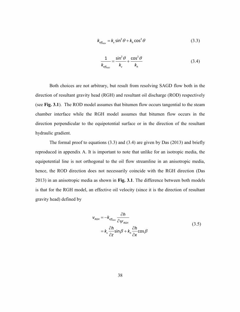
38
2 2sin cos
RGHeff v hk k k (3.3)
2 21 sin cos
RODeff v hk k k
(3.4)
Both choices are not arbitrary, but result from resolving SAGD flow both in the
direction of resultant gravity head (RGH) and resultant oil discharge (ROD) respectively
(see Fig. 3.1). The ROD model assumes that bitumen flow occurs tangential to the steam
chamber interface while the RGH model assumes that bitumen flow occurs in the
direction perpendicular to the equipotential surface or in the direction of the resultant
hydraulic gradient.
The formal proof to equations (3.3) and (3.4) are given by Das (2013) and briefly
reproduced in appendix A. It is important to note that unlike for an isotropic media, the
equipotential line is not orthogonal to the oil flow streamline in an anisotropic media,
hence, the ROD direction does not necessarily coincide with the RGH direction (Das
2013) in an anisotropic media as shown in Fig. 3.1. The difference between both models
is that for the RGH model, an effective oil velocity (since it is the direction of resultant
gravity head) defined by
sin cos
RGHRGH eff
RGH
v h
hv k
h hk k
z x
(3.5)

39
is used for its derivation. Here, is the direction parallel to the steam chamber interface.
The resultant gravity head can in turn be resolved in the horizontal and vertical direction
as:
cosRGH
h h
x
(3.6)
sinRGH
h h
z
(3.7)
Substituting2 2sin cos
RGHeff v hk k k obtained by projecting vk and hk in the direction of
the gravity head inclined at an angle (see appendix A) together with equation (3.6) and
(3.7) in the expression for the velocity yields:
cos sinRGH H v
h hv k k
x z
(3.8)
For the ROD model, an effective gravity head (in the direction of resultant oil discharge)
is defined by
sin cosROD
h h h
z x
(3.9)
corresponding to the angle subtended by the resultant oil discharge direction. The
components of the oil velocity are given by
cosx RODv v (3.10)

40
sinz RODv v (3.11)
Substituting2 21 sin cos
RODeff v hk k k
obtained by projecting vk and hk in the direction of the
oil discharge inclined at an angle (see appendix A) together with equations (3.9) to
(3.11) for the velocity and gradient expressions yields:
cos sin
H vROD
k kh hv
x z
(3.12)
Comparing equations (3.8) and (3.12) reveals why the RGH and ROD models will give
different bitumen rates.
Determining which of the two expressions would give a more accurate
representation of the SAGD recovery performance is difficult. All analytical (and semi-
analytical) SAGD models such as Butler et al.’s (1981) original model implicitly assume
the RGH model as they obtain bitumen rates as a function of the resultant gravity
potential gradient in the direction parallel to the steam chamber interface.
An implicit assumption made in both these models accounting for permeability
anisotropy is that at every specific time, effk is a constant for all fluid streamlines parallel
to the steam chamber interface. This is clearly seen from a step in the derivation of
Butler’s equation (2.1) where the production rate q is written as:
0
1 1sineff
R
q k g d
(3.13)

41
where the coordinate is perpendicular to the chamber wall. We speculate that in the
presence of anisotropy, the derivation of flow rate is written better as:
0
1 1sin eff
R
q g k d
(3.14)
since effk will vary ahead of the steam chamber interface. However, for most bitumen
reservoirs, viscosities are high enough such that the activated volume ahead of the steam
chamber front is small, and hence (3.13) can be used without much error.
In Fig. 3.3, we plot the difference in effective permeability using both models for
varying steam chamber angles (to the horizontal axis) and anisotropy ratio. The
difference in effective permeability using both models is more pronounced at lower steam
chamber angles and anisotropy ratios reaching a value of more than 81% for anisotropic
ratio of 0.1 and steam chamber angle of 20 degrees. Hence, we should expect some
significant difference in results from modeling the effect of anisotropy using both the
RGH and ROD models with any Butler type model. It is important to note here that Azad
and Chalaturnyk (2010) used the ROD model in their work. It will be helpful if a
recommendation can be made as to which model to use, but we will defer to comment on
such recommendation until we validate the models using numerical simulation.

42
Figure 3.3: Plot of the % difference between the RGH and ROD models
3.1.1 Computing Oil Production Rate Accounting for Permeability Anisotropy
Using the RGH model and substituting (3.3) into (2.1) gives
2 22 sin cos
RGH
o v h T
o
os
S k k g Hq
m
(3.15)
From (3.2) and writing sW t at any given time instant as sW , we get
2
2
2 2cos s
s
W
W H
(3.16)
2
2
2 2sin
s
H
W H
(3.17)
Substituting (3.16) and (3.17) into (3.15) gives
0
10
20
30
40
50
60
70
80
90
0 0.2 0.4 0.6 0.8 1
Effe
ctiv
e Pe
rmea
bilit
y di
ffer
ence
be
twee
n th
e R
GH
and
RO
D m
odel
s, %
Anisotropy ratio (Kv/Kh)
20 degrees
40 degrees
60 degrees
80 degrees

43
2 2
2 22
RGH
v h so T
so
os
k H k WS g H
W Hq
m
(3.18)
We have assumed that the steam chamber during horizontal growth is an inverted
triangle, then, similar to Reis’s (1992) development, mass balance gives
1
2o o s
dq S HW
dt
(3.19)
Combining (3.18) and (3.19) gives
2 2
2 28 RGH
RGHRGH
v h s
T
ss
o os
k H k Wg
W HdW
dt S Hm
(3.20)
The constant “8” in (3.20) is a consequence of using Butler’s original equation
(2.1). If we had used Reis’s model (1992), the constant would be “5” and similarly for
other models. We will replace this value with the constant “C2”. As in the previous works
by Reis (1992) and others, C2
is basically a correction for multiphase flow that occurs at
the edge of the steam chamber. It accounts for the retardation in the expansion of the
steam chamber due to the presence of condensed water at the edge of the steam chamber.
Non-dimensionalizing (3.20) yields
2
2 1RGHRGH
RGH
v h sDsD
D sD
k k WdWC
dt W
(3.21)

44
where
3
h TD
o os
k gt t
S m H
(3.22)
ssD
WW
H (3.23)
The corresponding non-dimensional form of the rate equation (3.19) is:
1
2
2
1
1
RGH
RGH RGH
RGH
k RGHvkh
v
h
sD
o v h sDDoD
sDo sD
kD
k
dW
q k k Wdtq
dWq Wdt
(3.24)
Similarly, using the ROD model and repeating the above procedure with (3.4)
substituted into (3.1) yields:
2 22 sin cos
ROD
o v h v h T
o
os
S k k k k g Hq
m
(3.25)
Substituting (3.16) and (3.17) into (3.25), the rate of growth of an inverted triangular
chamber yields:
2
1
2
1ROD ROD
ROD
sD sD
D vsD
h
dW WC
dt kW
k
(3.26)

45
1
2
1
2
1ROD ROD
ROD
KvKh ROD
o sD
oD
o vsD
h
q Wq
q kW
k
(3.27)
Equations (3.21) and (3.26) are non-linear ordinary differential equations (ODE’s) and
can be integrated analytically to give complex elliptic functions that will be difficult to
evaluate. We will rather solve (3.21) and (3.26) by finite differences. We will also utilize
the implicit finite-difference scheme due to its unconditional stability criterion and hence
overcome solution difficulties with the elliptic functions. Discretizing (3.21) and (3.26) in
such a manner gives
21
1
21 1
RGH
RGH RGH
RGH
nv h sDn n
sD sD Dn
sD
k k WW W C t
W
(3.28)
21
1
12
1
1ROD
ROD ROD
ROD
nsDn n
sD sD D
n vsD
h
WW W C t
kW
k
(3.29)
In order to access the impact of anisotropy on the steam chamber expansion, it
might be useful to compute the ratio:
1
D
DD
Dkvkh
S
S
S
WW
W
(3.30)

46
that is the ratio of the anisotropic steam chamber expansion to the isotropic case. The
isotropic steam chamber expansion is obtained from (3.21) or (3.26) by integrating the
corresponding expressions after substituting 1v hk k
1
Dkvkh
S DW Ct
(3.31)
Substituting (3.31) into (3.30) gives
D
DD
S
S
D
WW
Ct (3.32)
3.1.2 Model Validation
We will use numerical simulation and the CMG – STARSTM
non-isothermal
compositional simulator to validate our model for anisotropy during horizontal growth
for the SAGD process. To be successful, we will have to eliminate all physics not
accounted for in the Butler models (Roger M. Butler 1991) and are described below;
a. No overburden heat losses: The amount of heat injected during SAGD is used to
raise bitumen temperature as well as heat up the reservoir overburden. At steady
state, the amount of steam injected is the total required to raise the bitumen
temperature as well as to account for heat loss to the overburden. This is the
scenario assumed by Reis (1992). However, a fully numerical model is transient
and will generally couple both these heat transfer processes. We will eliminate
this effect in our validation by assuming zero overburden heat losses.
b. Zero pressure gradient other than gravity: There are situations where it is
desirable to operate the SAGD process under a pressure gradient other than

47
gravity (Edmunds and Gittins 1993). However, the Butler models does not take
any additional pressure gradient other than gravity into account, hence, in our
validation, we will operate the horizontal wells under zero pressure gradient.
c. Zero multiphase flow effects and (numerical) dispersion: As stated in the
literature review, the Butler models were derived assuming only single phase non-
isothermal flow of the bitumen phase. Several constants and fudge factors have
historically been used to account for multiphase flow effects in most Butler type
analytical models. However, multiphase flow is coupled to permeability
anisotropy as we will show in subsequent sections and in the absence of a reliable
model to quantify such coupling, multiphase flow effects should be eliminated in
our validation. To do this, we will use straight line relative permeability curves
with zero end points. This will eliminate multiphase flow effects parallel to the
steam chamber interface. We minimized numerical dispersion by using very small
grid sizes within reasonable computational limits and will discuss its effect in the
results section. In chapter 4, we will present a model that accounts for multiphase
flow ahead of the steam chamber interface by coupling the mass and energy
conservation equations. Table 3.1 gives the reservoir parameters used for the
validation study.

48
Table 3.1: Showing the values of reservoir parameters used in the anisotropic model
validation
Reservoir Parameter Value
Horizontal Permeability, hk 7000 mD
Thermal diffusivity, T 1.15942 x 10⁻⁶
m2/s
Viscosity, B TAe
A 8.13 x 10⁻⁹
cp
B 8871.026 K
m 5.2546
Porosity, 0.33
oS 1
Bitumen density 980 kg/m3
Reservoir thickness, H 25.7186 m
Number of grid block in x direction, xN 149
Number of grid block in y direction, yN 2
Number of grid block in z direction, zN 49
Size of grid block in x direction, x 0.5253441 m
Size of grid block in y direction, y 10 m
Size of grid block in z direction, z 0.5253441 m
The Butler parameter m was computed by performing the integration in (2.2).

49
3.2 Model Development – Multiple Layered Reservoirs
The above models are only valid for single layered reservoirs where the v hk k
ratio is constant throughout the reservoir. However, most bitumen reservoirs are not
single – layered and the v hk k ratio is usually spatially varying. In the limit of the
reservoir being layered i.e. having layers of rocks exhibiting different permeability
anisotropies, the above model can be extended to account for the effect of such multi-
layered reservoirs.
Consider the SAGD process during horizontal growth for a layered reservoir as
shown in Fig. 3.4
Figure 3.4: Schematic of an idealized SAGD steam chamber during horizontal growth
for a layered reservoir

50
Both the RGH and ROD models apply. From Fig. 3.4 and noting that the Butler type
models assume quasi-steady state flow, then the following relationship holds
1 2 3...
No o o o oq q q q q (3.33)
Equation (3.33) basically treats each layer as a separate SAGD process and has its
basis on the assumption of quasi-steady state i.e. the fluid entering any layer exits the
layer without any accumulation. Hence if conditions exist that makes Butler’s model
valid (high viscosity oil, injection at reservoir pressure, etc.), then (3.33) is also valid. For
each layer, (3.15) can be written for the RGH model as
2 22 sin cos
i i
iRGH
o v h T i
o
os
S k k g Hq
m
1,2,...,i N (3.34)
From (3.1), (3.33) and (3.34) we get
2 2
1
sin cosi i
RGH
N
v h ii
eff
k k H
kH
1,2,...,i N (3.35)
If we assume that the steam chamber angle to the horizontal is the same for each
layer (this assumption is strictly valid for gravity stabilized flows), we can use the results
of the previous section that gives the angle as a function of reservoir and steam chamber
dimensions which will be the same as (3.16) and (3.17) to give the effective
permeabilities as

51
2 2
2 2RGH
v h seff
s
k H k Wk
W H
(3.36)
which also applies to each layer due to the principle of geometric self-similarity to give
2 2
2 2i i
iRGH
v h s
eff
s
k H k Wk
W H
1,2,...,i N (3.37)
In (3.37), we have used the assumption of an invariant with respect to each
layer. As noted earlier, this assumption breaks down in the presence of high permeability
streaks, impermeable barriers or strong capillary heterogeneities since for such situations,
gravity will likely not be strong enough to stabilize any advancing front orthogonal to the
drainage direction.
Substituting (3.37) into (3.35) and non-dimensionalizing sW gives
2
21
1
1RGH i i RGH i
RGH
N
eff v h sD DisD
k k k W HW
1,2,...,i N (3.38)
where i
iD
HH
H 1,2,...,i N (3.39)
andDSW is given by (3.23). Substituting (3.38) into (3.1) and non-dimensionlaizing oq gives
1
2
1
2
1
1
RGH i i
RGH
RGH
KvRGH i iKh i
Nv
sD h Di ho i
oD N
osD h D
i
kW k H
kqq
qW k H
1,2,...,i N (3.40)

52
Combining (3.1), (3.38) and (3.19) in dimensionless space gives the corresponding rate of
growth of the steam chamber as:
2
1
2
1
1
RGH i i
RGH
RGH i i
Nv
sD h Di hsD i
N
DsD h D
i
kW k H
kdWC
dtW k H
1,2,...,i N (3.41)
where
1
1
2i i
kvkh i
N
o T h Di
o
os
S g H k H
qm
1,2,...,i N (3.42)
13
i i
N
T h Di
D
o os
g k H
t tS m H
1,2,...,i N (3.43)
In (3.42), we have used the same analysis in (3.35) to (3.40) for its derivation but for
isotropic conditions. In the special limit where the horizontal permeability is the same
across the layers (3.40) to (3.43) becomes
1
2
1
2 1
RGH i
RGH
RGH
K RGHvKh i
Nv
sD Di ho i
oD
o sD
kW H
kqq
q W
1,2,...,i N (3.44)

53
2
1
2 1
RGH i
RGH
RGH
Nv
sD Di hsD i
D sD
kW H
kdWC
dt W
1,2,...,i N (3.45)
1
2kvkh i
o h To
os
S k g Hq
m
(3.46)
The assumption of constant horizontal permeability across layers is not necessary but
used here to reduce the amount of parameters required to solve the model. Similar
derivations as above using the ROD model yields
1
2
11 2
1
1 i i
ROD
ROD
ROD
ROD
Kvi iKh i
Nh D
sDi
vsD
o h ioD N
oh D
i
k HW
kW
q kq
qk H
1,2,...,i N (3.47)
2
11 2
1
1 i i
ROD
ROD
ROD
i i
Nh D
sDi
vsD
sD h iN
Dh D
i
k HW
kW
dW kC
dtk H
1,2,...,i N (3.48)
If we also assume the horizontal permeability to be the same across the layers, (3.47) and
(3.48) becomes

54
1
2
11 2
1ROD i
ROD ROD
KvKh RODi
No D
oD sDio v
sD
h i
q Hq W
q kW
k
1,2,...,i N (3.49)
2
11 2
1ROD i
ROD
ROD
NsD D
sDiD v
sD
h i
dW HC W
dt kW
k
1,2,...,i N (3.50)
Equations (3.40) to (3.50) reveal that the effect of anisotropy on recovery from
multi-layered reservoirs during horizontal growth of the SAGD process is not only
dependent on the vertical permeability, but also on the combination of vertical
permeability and thickness of each layer. This renders the use of variance based reservoir
heterogeneity measures like the Dykstra-Parsons or Lorenz coefficient to characterize the
SAGD response at best fortuitous as seen in the unexplainable results of Kamath et al.
(1993) discussed in chapter 2. However, it will be interesting to attempt such
characterization by determining a simple and yet suitable parameter for the unique flow
geometry of the SAGD process. A clue to this can be seen from (3.40) to (3.50) where it
can be reasonably hypothesized that all layered reservoirs having an equivalent
anisotropy ratio v h eqk k defined as
1
1
i
i
N
v h h iii
v h Neq
h ii
k k k H
k k
k H
1,2,...,i N (3.51)
should have the same dimensionless bitumen rate response during the horizontal SAGD
growth phase. If each layer has the same horizontal permeability, (3.51) becomes

55
1
i
N
v h v h Deq ii
k k k k H
1,2,...,i N (3.52)
It should be understood that the equivalent permeability model is just a way to convert
the multi-layered model to the single layer model. We will use (3.52) to verify the above
hypothesis in an example problem below.
3.2.1 Example Problem
In this section, we will consider two cases – a high permeability anisotropy case
(left table) and a low permeability anisotropy case (right table) for a 6 layered reservoir.
The reservoir parameters for both cases are given in Table 3.2. We have chosen both
cases to have the same distribution for the thickness of each layer for convenience. We
are also assuming for both cases that the horizontal permeability is the same in all the
layers.

56
Table 3.2: The v hk k ratio for each layer and the dimensionless thickness distribution.
The higher permeability anisotropy case is shown on the left and the lower
permeability anisotropy case is shown on the right.
v h ik k
iDH
0.05 0.25
0.01 0.1
0.1 0.05
0.04 0.2
0.02 0.15
0.07 0.25
Based on the data in Table 3.2, and using (3.52), the equivalent anisotropy ratio is
calculated for both cases as
0.047v h eqk k (3.53)
for the high permeability anisotropy case and
0.655v h eqk k (3.54)
for the low permeability anisotropy case.
v h ik k
iDH
0.6 0.25
0.7 0.1
1 0.05
0.5 0.2
0.4 0.15
0.9 0.25

57
3.3 Results and Discussion
Fig. 3.6 shows the plot of the dimensionless oil production rate as a function of
dimensionless time for the RGH model. Notice that for all practical purposes, the effect
of anisotropy disappears at 3Dt for all anisotropy ratios. This is a very interesting result
because it suggests that there exists a combination of reservoir and fluid parameters for
which the effect of anisotropy becomes unimportant at times that are small enough to be
ignored. This is however not the case if the ROD model is used especially for lower
anisotropy ratios as seen in Fig. 3.9. Both models reveal that the general effect of
anisotropy is to introduce a time component to the maximum SAGD oil rate. Figs. 3.6
and 3.9 exhibit a discontinuity at 0Dt and this is because at the start of the SAGD
horizontal growth phase, there will be a finite non-zero rate response. Also, form Figs.
3.6 and 3.9 and for 0.01v hk k there is a dramatic difference between the RGH and the
ROD models. The reason for this can be understood better from Fig. 3.3 where the
difference in effective permeabilities can be as high as 90% depending on the steam
chamber angle.
Figs. 3.7 and 3.10 plots the dimensionless steam chamber half width for both the
RGH and ROD models respectively and we see that while the effect of anisotropy on
steam chamber expansion is short-lived (about 1Dt for 0.01v hk k ) for the RGH model,
the ROD model predicts that anisotropy ratios less than 0.1 is likely to impact the rate of
growth of the steam chamber through-out the duration of the process.
Figs. 3.8 and 3.11 show more clearly the loss in size of the steam chamber with
time due to anisotropy. While the RGH model predicts that given sufficient time (and if
the reservoir aspect ratio allows), the steam chamber will recover to its isotropic size for
all anisotropic ratios. For lower values of anisotropy ratio, the time after which the

58
chamber geometry will coincide with that for the isotropic case may be substantially
large and it may be that the physical boundaries of the layer may be experienced prior to
that time. The ROD model predicts that convergence to the isotropic case might happen
at infinite time for 0.01v hk k . This result might lead to the conclusion that the ROD
model is the more physically appropriate choice since it is generally agreed that the
SAGD process will fail for any reservoir with such low anisotropic ratios because the
steam chamber will simply not grow. It is important to note however, that the results we
show here are only strictly valid during horizontal growth of the steam chamber and
hence, implicit in them is the assumption that the steam chamber has already grown to
reach the top of the reservoir. Figs. 3.12 to 3.14 are comparison plots and reveal both
models are indistinguishable when 0.7v hk k .
Fig. 3.15 shows the validation plot comparing both the RGH and the ROD models
with numerical simulation results using CMG-StarsTM
. The input model for the numerical
simulation is given in Table 3.1. As discussed earlier, modifications have been proposed
to Butler’s model to account for multiphase flow effects. However, these modifications
are mostly empirical and most likely have to be calibrated against the actual
characteristics of the process as represented in a simulation result or as measured in the
field. For this reason, in Fig. 3.15 we calculated a multiphase flow factor for the isotropic
case by dividing the simulation average bitumen rate with the theoretical Butler model
rate obtained using (2.1). This calibration multiphase flow factor was subsequently used
for all v hk k ratios. However as observed in Fig. 3.15, the application of this multiphase
flow factor results in a poor match between the simulation and semi-analytical results.
This can be explained further by writing the orthogonal components of the effective
permeabilities in the presence of anisotropy for both the RGH and ROD models as

59
2 2cos sinRGHeff v hk k k
(3.55)
2 21 cos sin
RODeff v hk k k
(3.56)
whereRGHeffk and
RODeffk are the effective permeabilities for both the RGH and ROD
models orthogonal to the steam chamber interface.
From (3.55) and (3.56) we see that the effective permeability orthogonal to the
steam chamber interface will decrease with a decrease in the v hk k ratio which will
generally give lower multiphase flow factors at lower v hk k ratios. Even though in chapter
4, we will describe a model accounting for multiphase flow during SAGD horizontal
growth, we have not coupled such to anisotropy in this dissertation. Hence, we will treat
the anisotropic multiphase flow factors as a history match parameter and the results are
shown in Fig. 3.16. An excellent match between our anisotropy models and numerical
simulation result is seen in Fig. 3.16 and the anisotropic multiphase flow factors used to
obtain the match is given in Table 3.3. Fig 3.16 also shows that the ROD model is more
accurate than the RGH model at lower v hk k ratios. It is important to note that in Fig.
3.16, we are only plotting the SAGD rates during horizontal growth from the numerical
simulation.
Figs. 3.17 to 3.19 reveal that the history matched multiphase flow factors shown
in Table 3.3 are not necessarily fudge factors. Fig. 3.17 shows the temperature profile
close to the end of the horizontal growth period for the isotropic case using the validation
parameters in Table 3.1. The plot shows that the heat transfer length scale varies from
about 1m at the top of the chamber to about 5m at the base of the chamber. Figs 3.18 and
3.19 give the water saturation profiles for the isotropic and 0.3v hk k cases respectively

60
and from which we see that the saturation diffusivity length scale is similar to the heat
transfer length scale and the degree of saturation diffusion for the anisotropic case is
slightly greater than that of the isotropic case, thereby giving rise to smaller multiphase
flow factors. It is important to note that saturation diffusion here is caused by numerical
dispersion and in chapter 4, we will show that saturation diffusion similar to that from
numerical simulation, is evident from laboratory and field scale recoveries but are rather
caused by the Marangoni or thermo-capillary effect.
There is however an alternative explanation to the mismatch of Fig. 3.15. The
mismatch between the simulation and semi-analytical results may be due to grid
orientation effects that are inherent in structured grid based finite difference simulators.
Due to the unique geometry of the SAGD process, the effective permeability parallel to
the steam chamber wall is always underestimated because of the stair-step flow that is
simulated on the grid. This effect is shown in Fig. 3.5 where the effective permeability
parallel to the steam chamber wall is driven largely by the vertical permeability (since we
have used a zero pressure gradient between the wells, the horizontal permeability effect
will be small and will only arise due to pressure perturbations in the simulation). This is a
consequence of not using the full permeability tensor in formulating the finite difference
equations in most commercial simulators. Even though we have used very small grid
sizes to minimize this effect, it is likely it was not eliminated. Also, using dynamic grid
refinement around the steam chamber interface didn’t help much as the structure of the
problem doesn’t change beyond a particular refinement level – beyond this point, what is
needed is a change in the grid orientation relative to the steam chamber interface and not
the grid size. To resolve this problem, and hence determine the more accurate model
between the RGH and ROD model will require either experimentation or a gridding
technique relatively insensitive to the grid orientation effect like the finite element

61
method (FEM). FEM has been applied to the SAGD process (Bogdanov et al. 2007), but
only for a homogenous reservoir.
Before the grid orientation issue is resolved, we recommend that any semi-
analytical model developed to analyze the effect of anisotropy on SAGD performance
should include sensitivities to using both the RGH and ROD models. If such sensitivities
reveal significant differences in recovery performance, then a choice will have to be
made taking into account the nature of the phenomenon itself, and at the very least, the
difference in results using both models can be used to inform uncertainty due to
anisotropy.
vk
vk
vk
Figure 3.5: Showing a finite difference based grid orientation during SAGD horizontal
growth with an effective permeability parallel to the steam chamber wall
similar to the vertical permeability
injector
producer
steam chamber interface
grid block

62
Table 3.3: Showing the multiphase flow factor for each v hk k ratio suitable for comparing
the semi-analytical model with numerical simulation results
v hk k ratio Multiphase Flow Factor
1 0.76
0.7 0.61
0.3 0.46
Figs. 3.20 to 3.22 show the results for the layered models which give similar results as
the single layer case as at high equivalent anisotropy ratios, the RGH and ROD models
are indistinguishable approaching the asymptotic limit of the isotropic case for 3Dt ,
while at low equivalent anisotropy ratios, significant differences between both models
exist. They also reveal that the equivalent anisotropy ratio v h eqk k is an exact
characterization parameter for the RGH model, but is not for the ROD model especially
at low v h eqk k ratios. This is because v h eq
k k was derived using the Butler’s model
which in turn was derived implicitly assuming the RGH model, not the ROD model.
Since this work was entirely done in dimensionless space, Fig. 3.6 or 3.9 can be
used as type curves to predict the effect of anisotropy on SAGD rates. As mentioned
earlier, these curves are strictly valid for the horizontal growth phase of the steam
chamber but they can still be used with caution for both the vertical growth and the
depletion phases with a slight modification to the governing equations. This modification
includes rescaling the models presented in this chapter by using H H t (with the
respective definitions for both the vertical growth and depletion phases) instead of H .
This will require an elaborate procedure different from (especially for the depletion

63
phase) that described by Llaguno et al. (2002) and which is beyond the scope of this
dissertation.
Figure 3.6: Plot of dimensionless rate vs. dimensionless time for the RGH model
Figure 3.7: Plot of dimensionless steam chamber half width vs. dimensionless time for
the RGH model

64
Figure 3.8: Plot of ratio of anisotropic to isotropic dimensionless steam chamber
expansion vs. dimensionless time for the RGH model
Figure 3.9: Plot of dimensionless rate vs. dimensionless time for the ROD model

65
Figure 3.10: Plot of dimensionless steam chamber half width vs. dimensionless time for
the ROD model
Figure 3.11: Plot of the ratio of anisotropic to isotropic dimensionless steam chamber
expansion vs. dimensionless time for the ROD model

66
Figure 3.12: Comparison plot of dimensionless rate vs. dimensionless time for the RGH
and ROD models
Figure 3.13: Comparison plot of dimensionless steam chamber half width vs.
dimensionless time for the RGH and ROD model

67
Figure 3.14: Comparison plot of the ratio of anisotropic to isotropic dimensionless steam
chamber expansion vs. dimensionless time for the ROD model
Figure 3.15: Comparison plot of bitumen rate vs. time for the RGH, ROD and numerical
simulation models for constant multiphase flow calibration factors
0
5
10
15
20
25
30
35
40
45
50
0 20 40 60 80 100 120 140 160 180
Bit
um
en r
ate
q (
m3/d
ay)
time (days)
q_RGH_kv/kh = 0.7
q_RGH_kv/kh = 0.3
q_ROD_kv/kh = 0.7
q_ROD_kv/kh = 0.3
q_simulation_kv/kh = 1
q_simulation_kv/kh = 0.7
q_simulation_kv/kh = 0.3

68
Figure 3.16: Comparison plot of bitumen rate vs. time for the RGH, ROD and numerical
simulation models for varying multiphase flow calibration factors
Figure 3.17: Temperature profile from numerical simulation validation for 1v hk k
0
5
10
15
20
25
30
35
40
45
50
0 20 40 60 80 100 120 140 160 180
Bit
um
en r
ate
q (
m3/d
ay)
time (days)
q_RGH_kv/kh = 0.7
q_RGH_kv/kh = 0.3
q_ROD_kv/kh = 0.7
q_ROD_kv/kh = 0.3
q_simulation_kv/kh = 1
q_simulation_kv/kh = 0.7
q_simulation_kv/kh = 0.3

69
Figure 3.18: Water Saturation profile from numerical simulation validation for 1v hk k
Figure 3.19: Water Saturation profile from numerical simulation validation for
0.3v hk k

70
Figure 3.20: Comparison plot of dimensionless rate vs. dimensionless time for the
layered and equivalent RGH and ROD models
Figure 3.21: Comparison plot of dimensionless steam chamber half width vs.
dimensionless time for the layered and equivalent RGH and ROD models
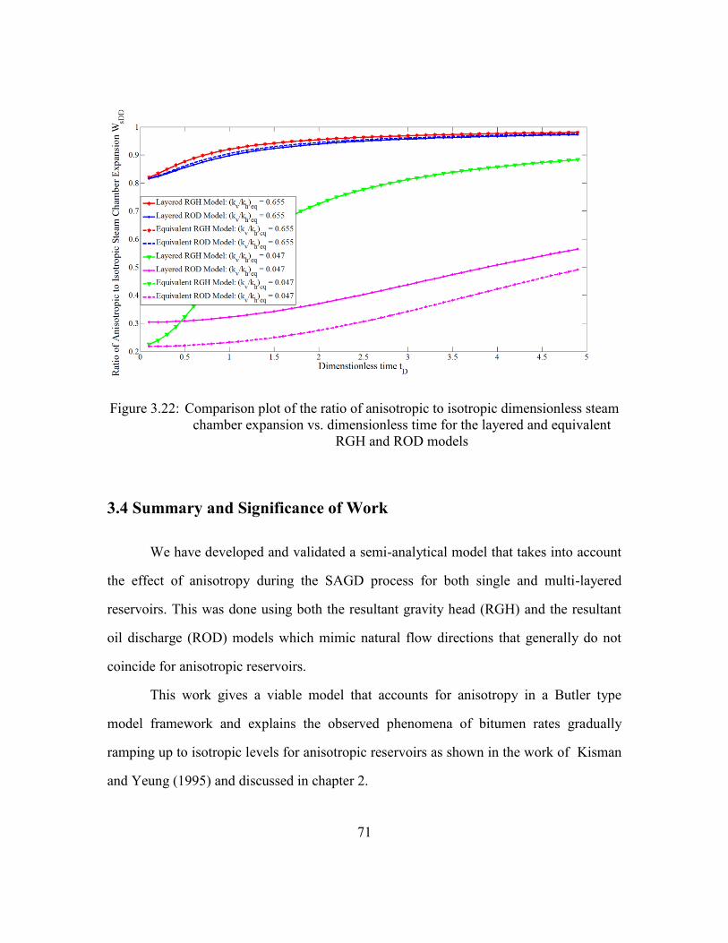
71
Figure 3.22: Comparison plot of the ratio of anisotropic to isotropic dimensionless steam
chamber expansion vs. dimensionless time for the layered and equivalent
RGH and ROD models
3.4 Summary and Significance of Work
We have developed and validated a semi-analytical model that takes into account
the effect of anisotropy during the SAGD process for both single and multi-layered
reservoirs. This was done using both the resultant gravity head (RGH) and the resultant
oil discharge (ROD) models which mimic natural flow directions that generally do not
coincide for anisotropic reservoirs.
This work gives a viable model that accounts for anisotropy in a Butler type
model framework and explains the observed phenomena of bitumen rates gradually
ramping up to isotropic levels for anisotropic reservoirs as shown in the work of Kisman
and Yeung (1995) and discussed in chapter 2.

72
This work will find great utility in proxy based history matching of the SAGD
process and also in optimal well spacing design because it reveals that if the well spacing
is such that you are past the horizontal growth phase by dimensionless time 3Dt for any
given anisotropy ratio, then your wells will probably never produce at its maximum
possible rate. Economics will ultimately drive the decision of well spacing but
understanding how anisotropy influences it is an invaluable contribution of this work.
This work has also helped illuminate on the weakness of grid based finite
difference simulators in capturing the correct effective permeabilities for the propagation
of fluid interfaces that are inclined to the simulator’s grid orientation such as observed in
the SAGD process. More research still needs to be done to understand the grid orientation
effect as it relates to anisotropic SAGD flow.

73
Chapter 4: The Effect of Heat Transfer on Capillarity during SAGD
By solving a 1-D heat conservation equation for single phase flow along the
steam chamber wall, Butler et al. (1981) derived their classical SAGD model. Their
equation has excellent predictive capability at experimental scales but performs poorly at
field scales. Several authors have postulated that multiphase flow along the steam-
bitumen boundary that was not accounted for in the Butler’s original model has an
important impact on recovery. They have proposed rate multipliers to bring the model
predictions closer to observations and related these multipliers to multiphase flow effects,
but in practice, the multipliers seem to vary for each reservoir or experiment. Another
reason why the Butler models perform poorly at field scales is because it only takes into
account flow due to gravity neglecting other pressure gradients. However, at field scales,
other pressure gradients are known to exist (Ito and Suzuki 1999).
Recently, by making the prior assumption that fluid saturations ahead of the steam
chamber vary linearly with temperature, Sharma and Gates (2010b) derived a SAGD
equation that accounts for multiphase flow ahead of the steam chamber, which performs
excellently at field scales but poorly at experimental scales. In this work, we proceed by
decomposing capillary pressure change into its temperature and saturation components.
Our premise is that though capillary pressure changes due to saturation, these changes are
likely to be negligible given the unconsolidated nature of the reservoir. However, the
large temperature changes associated with the process can induce significant changes to
the interfacial tension between the oil and water and that in turn can induce significant
capillary pressure changes. This phenomenon is the classical Marangoni (or thermo-
capillary) effect where interfacial tension driven flows are triggered by temperature (or
concentration gradients) (Lyford et al. 1998), (Flock et al., 1986). We also show how the

74
Marangoni number can be used to characterize this effect. At low Marangoni numbers
(typical of experimental scales) we get the Butler solution while at high Marangoni
numbers (typical of field scales), we approximate the Sharma and Gates solution. The
entire modeling was done in dimensionless space so our results can be used as a fast
SAGD predictive model within a proxy-based history matching process.
4.1 Model Development
We now present the detailed development of our model that quantifies thermo-
capillary behavior during SAGD. Note that we interchangeably use the term thermo-
capillarity for what is known as the Marangoni effect through this chapter and the rest of
the dissertation.
4.1.1 Transport equations in a fixed frame
The SAGD process is a moving boundary problem, but we present the basic mass
and energy transport equations in a fixed coordinate (Eulerian) frame in this section and
then transform these equations into a moving coordinate (Langrangian) frame in the next
section. There are three phases flowing simultaneously during SAGD – water vapor,
liquid water and bitumen – however, water vapor will usually be non-wetting in the
porous medium, hence, it will not imbibe into the pore space containing bitumen. The
wetting phase – usually liquid water – will preferentially imbibe into the pore space
containing the intermediate wetting phase – bitumen. Furthermore, water vapor will
condense at the steam chamber boundary, and ahead of this boundary, no vapor remains.
This implies that for all practical purposes, it suffices to study the two-phase (liquid water
and bitumen) problem when studying capillary imbibition during SAGD. We assume in

75
the foregoing analysis that water is the wetting phase. The conservation equations are
now presented.
Mass conservation for the water phase is given as
0w w w wSt
u (4.1)
and for the bitumen phase as
0o o o oSt
u (4.2)
The velocities are given by Darcy’s law
rww w w w w w
w
kkp p
u g g (4.3)
roo o o o o o
o
kkp p
u g g (4.4)
Pressure in the water and bitumen phases are related through capillary pressure
,o w c wp p P S T (4.5)
Note that capillary pressure is expressed explicitly as a function of both wetting phase
saturation as well as temperatureT . If we assume constant phase densities for the water
and bitumen phases, (4.1) and (4.2) becomes

76
0w wSt
u (4.6)
0o oSt
u (4.7)
Adding (4.6) and (4.7) and noting that for two phase flow
1o wS S (4.8)
we can derive:
0 u (4.9)
where o w u u u is the total velocity which is given by
o cp P u g (4.10)
where o w is the total mobility and we have assumed that o w which is a
good assumption for heavy oils. Substituting (4.3) and (4.4) into (4.6) and (4.7)
respectively gives
0w w wS p
tg (4.11)
0o o oS p
tg (4.12)

77
If we assume that water is always a connected phase, we can choose to take the pressure
in the water phase as the reference pressure variable, hence wp p . Using this definition
and assuming constant porosities, (4.5), (4.11) and (4.12) can be written respectively as
0w
w
Sp
tg (4.13)
0o
o c
Sp P
tg (4.14)
The next transport equation to consider is that of energy. In the absence of the other
phenomena like emulsification and well bore flow effects, the only heat transfer
mechanism operating during SAGD is thermal conduction. Hence, energy conservation
for the two phase system and porous media gives
1
0
so o w w s
THo o w w o o c
TS C S C C
t
kC C p T C P T T
g
(4.15)
where THk is the thermal conductivity of the reservoir and oC , wC and sC are the specific
heat capacities of the bitumen, condensate and reservoir solid rock phases. Equations
(4.13), (4.14) and (4.15) are the transport equations in a fixed frame. As is, these
equations can be solved using a numerical scheme (by making finite difference
approximations). However, our goal is to derive an analytical or semi-analytical solution

78
for the above. For this, we will transform the same set of equations to a moving reference
frame.
4.1.2 Transport equations in a moving reference frame
In a moving reference frame (see appendix B) in which we assume that the steam
chamber is expanding in a quasi-steady state manner (Butler, 1991), (4.13), (4.14) and
(4.15) become
0w wS p U g' (4.16)
0o o cS p P U g' (4.17)
1
0
so o w w s
THo o w w o o c
S C S C C T
kC C p T C P T T
U
g'
(4.18)
where ,T
is the gradient operator in the moving reference frame and U is the
velocity with which the steam-bitumen interface moves (see Fig. 4.1). Flow in the
direction parallel to the front ( direction) will be fast relative to that in the direction
orthogonal to the front ( direction) and hence, we can neglect variations in saturation
pressure (note that we have assumed equal densities for water and bitumen, hence gravity
will not be a factor here) and temperature in the direction parallel to the front. This allows
us to ignore the gradients in the direction and write:

79
sin 0wf w
dS d dpU g
d d d
(4.19)
sin 0o cf o
dS dPd dpU g
d d d d
(4.20)
1
sin 0
sf o o w w s
c THo o w w o o
dU S C S C C T
d
dP kd dp dTC C g T C T
d d d d
(4.21)
Figure 4.1: Schematic of the SAGD steam chamber showing important flow directions
and the steam chamber front velocity vector
where fU is the front velocity in the direction. Since we have assumed fU is independent
of ,(4.19), (4.20) and (4.21) can be integrated with respect to between an arbitrary

80
value (corresponding to any location away from the interface) and (corresponding to
the undisturbed reservoir) to yield the mass and energy balances within a given volume of
the reservoir as
sinw
wi
S
f w w
S
dpU dS g
d
(4.22)
1
sino
wi
S
cf o o
S
dPdpU dS g
d d
(4.23)
,
,
1
sin
w
wi R
S T
sf s o o w w
S T
c THo o w w o o
U d C S C S C T
dP kdp dTC C g T C T
d d d
(4.24)
The right hand sides of these equations are fluxes that approach zero when approaches
infinity. In this limit, wS approaches wiS , oS approaches1 wiS andT approaches RT , the
reservoir temperature. The integration is thus straightforward and gives:
sinf w wi w
dpU S S g
d
(4.25)
1 sin cf o wi o
dPdpU S S g
d d
(4.26)

81
1
sin
sf o s R w o w wi R
c THo o w w o o
U C C T T C C S T S T
dP kdp dTC C g T C T
d d d
(4.27)
Summing (4.25) and (4.26) gives
0 sin co w o
dPdpg
d d
(4.28)
Simplifying (4.28) gives
sin o c
o w
dPdpg
d d
(4.29)
Substituting (4.29) in (4.25), (4.26) and (4.27) allows for the elimination of the pressure
gradient term to give
cf w wi
dPU S S
d
(4.30)
1 s c TH
f o s R w o w wi R w o
dP k dTU C C T T C C S T S T C C T
d d
(4.31)
where
, ,w o
w wo w s
kS T f S T (4.32)

82
in which
s o sT T (4.33)
rw ro s
ro w rw o
k kf
k k
(4.34)
Expanding (4.32) using Corey relative permeability curves gives
1,
1
b a
rwro wD rocw wD sw a b
srocw wD w rwro wD o
k S k S kS T
k S k S (4.35)
where a and b are the Corey exponents of oil and water phases respectively and
1
w wcwD
wc or
S SS
S S
(4.36)
Bitumen viscosities are usually order of magnitudes higher than water viscosities
throughout the temperature space, hence – for all practical purposes
1b a
rwro wD o rocw wD wk S k S (4.37)
Substituting condition (4.37) into (4.35) gives

83
1,
a
wD srocww
s o
Sk kS T (4.38)
Equation (4.38) implies a weak dependence of mobility on the water relative permeability
exponent b i.e. the curvature of the water relative permeability curve. It is interesting to
note that this weak dependence was also implicitly assumed albeit without proof in
Sharma and Gates (2010b).
The bitumen viscosity-temperature relationship can be approximated by (Butler
1991)
* m
s
o
T (4.39)
where
* R
s R
T TT
T T
(4.40)
Substituting (4.39) into (4.38) gives
*, 1
marocww wD
s
k kS T S T (4.41)
Equation (4.31) can be simplified further to give
Rf
T
T TdTU
d
(4.42)

84
where T is the reservoir’s thermal diffusivity and given as
THT
k
C (4.43)
with
1
1s s wi w wi oC C S C S C
(4.44)
The thermal diffusivity defined in (4.42) through (4.44) is quite different from the
apparent diffusivity of Sharma and Gates (2011) where wS was used in place of wiS in
(4.44), hence, their theory predicts that thermal diffusivity will be a function of the
current saturation state wS . The reason for this difference is that our model is one of
thermo-capillary counter-current imbibition (hence, the convective fluxes cancel out)
while Sharma and Gates (2011) explicitly accounted for condensate convection in their
model. Condensate convection ahead of the steam chamber front as a transport
mechanism during SAGD is still open for debate because even if the steam injection
pressure is higher than the original reservoir pressure, fluid streamlines are still expected
to be parallel to the steam chamber interface and hence, there should be no convective
flow orthogonal to the steam chamber interface (Edmunds 1999).
Capillary pressure will depend on both the wettability of the porous medium and
the interfacial tension between water and bitumen. These in turn will depend on
temperature (Flock et al., 1986), hence, we can write that

85
w
c wS T
dP dS dTP P
d d d (4.45)
The functions wS c w T
P P S and w
T c SP P T account for the effect of temperature on
interfacial tension and wettability and will be defined shortly. Substituting (4.41) and
(4.45) into (4.30) gives
*1w
marocw wwD S T f w wi
s
k k dS dTS T P P U S S
d d (4.46)
A complex non-linear relationship between the saturation and the temperature gradient is
indicated in (4.46). This is in distinct contrast to the assumption in Sharma and Gates
(2010b) that the saturation gradient is identical to the thermal gradient. Substituting
(4.42) into (4.46) and simplifying yields
*1 ww
w wi s R Twf ma
T Srocw wD S
S S T T PdSU
d Pk k S T P (4.47)
The system composed of (4.42) and (4.47) is a coupled system of two non-linear ordinary
differential equations. It can also be written in vector form as
d
d
Yb (4.48)
where

86
,T
wS TY (4.49)
and
*,
1 ww
T
w wi s R T Rf ma
T S Trocw wD S
S S T T P T TU
Pk k S T Pb (4.50)
where the superscript T is the transpose. From (4.50), we see that in the limit , both
b and the derivatives go to zero as expected, which is an important heuristic check on our
derivations. Another important observation from (4.50) is that the system of equations
cannot be solved if the front velocity – which appears at the right hand side of (4.50) – is
unknown. This is often generally the case, and in order to calculate it, an equation for the
interface motion is needed. Also, the front velocity will not be constant at all locations
within the interface as it will be dependent on its local curvature. Using the same
transformation as in Butler (1991) (which is basically the chain rule of differential
calculus) which follows from (4.42) as
Rf
T
T Td dU
d dT
(4.51)
Substituting (4.51) into (4.48) gives
*1 ww
T w wi sw T
maS
rocw wD S R
S SdS P
dT Pk k S T P T T (4.52)

87
Equation (4.52) is a non-linear ordinary differential equation that describes the
change of saturation with respect to temperature ahead of the steam chamber front and
reveals that such change (for non-isothermal multiphase flow) is a function of the
thermal, viscous and capillary properties of the flowing fluids and the porous medium.
Before we simplify (4.52), let us define some useful constitutive relations.
4.1.3 Constitutive equations
The first constitutive equation we will describe is that of capillary pressure itself.
Leverett (1941), defined the J function as
cosc w
T TP J S
k
(4.53)
where cP is the capillary pressure, is the interfacial tension and is the wetting angle. A
wetting angle of 0 corresponds to a medium that is fully water-wet. For solids that are
preferentially water-wet, the Leverett J function is a decreasing function of water
saturation. For this work, we will use the model for wJ S given by El-Khatib (1995)
because of its closed form and ease of computing its gradient:
1
4 2w
wD
J SS
(4.54)

88
where is a constant related to the tortuosity of the porous medium. Equation (4.54) is
simply a generalization of the Brooks-Corey model to account for tortuosity effects and
the numerator of (4.54) plays this role. Differentiating (4.54) with respect to wS yields
1
4 2
1w
wD wc or
J SS S S
(4.55)
It is important to state here that other J functions like that of Van Genuchten (1980) can
be used or even specific field data – if available – and it doesn’t change the analysis that
follows. However, we found that (4.54) and (4.55) are more stable numerically and
specific experimental or field data should first be fit with (4.54) – whenever possible –
and only when unsuccessful should more sophisticated models or raw data be used. The
change in wJ S with saturation is usually assumed to be instantaneous in porous media
flows and this assumption will be important in this analysis.
The general trend for interfacial tension is to decrease with temperature and this
can be described by the Eötvös’ correlation (Eötvös 1886) which assumes interfacial
tension to be a linearly decreasing function of temperature. This trend has also been
observed by other researchers (Flock et al., 1986), (Bowman 1967). In the absence of
thermodynamic data needed to use Eötvös’ equation and also to account for the
deviations from linearity frequently observed in experiments, we will write this
correlation as
* nR
R s
T (4.56)

89
where n is a positive constantR is the interfacial tension at reservoir conditions and s is
the interfacial tension at steam conditions. The form of (4.56) ensures that Eötvös’ rule is
obeyed when 1n and also accounts for deviations from linearity when 1n .
The next parameter to consider is wettability. We could write a similar
constitutive equation to (4.56) for the change in wettability with temperature, but this
would assume that wettability and interfacial tension change with temperature at the same
time-scale. This becomes important given the quasi-steady state assumption employed to
derive the equations. In the absence of any data validating such an assumption, we will
assume that wettability is constant throughout the recovery process.
4.1.4 Dimensionless saturation profile
Substituting (4.53) and (4.56) into (4.52) and rendering the resulting equation
dimensionless using the scaled variables (4.40) and
* w wiw
o
S SS
S
(4.57)
where
o oi orS S S (4.58)
we get
1** *1
* ** 1
R S
R R S
n
ww wm nn a
owDw
T nJ SdS N S
SdT S TJ S T (4.59)

90
where
1
1
cos
T S T S
g rocw c rocw
NM kk P k k
(4.60)
1cosg rocw
s
dM L T k k
dT (4.61)
R s
(4.62)
and L is a characteristic length scale. 1N is a dimensionless number that is the inverse of
the Marangoni number gM which relates thermal-interfacial tension effects to viscous
effects. We call 1N the thermo-capillary number with cP equal to the change in capillary
pressure due to temperature change. A further look at (4.59) reveals that the Marangoni
behavior during SAGD can be effectively characterized by the following dimensionless
functional relationship
*
1*, , , , , ,w
w f wD
dSf N a m n J S S
dT (4.63)
where
1wi wc
wD
wc or
S SS
S S
(4.64)
and

91
R S
f
R
(4.65)
is the fractional decrease of interfacial tension from the undisturbed reservoir to the steam
front. Also from (4.54) and (4.55), the effect of the Leverett J function wJ S and its
gradient wJ S can be effectively characterized by . Equation (4.63) then becomes
*
1*, , , , , ,w
f wD
dSf N a m n S
dT (4.66)
Note that from (4.59), (4.63) and (4.66) should also show a dependence on oS but oS is
not independent of wDS hence its seclusion from the functional relationship. Equation
(4.66) is sufficient to characterize the Marangoni effect on the SAGD oil rate. It is more
interesting to describe this effect in terms of a saturation-distance relationship rather than
the more abstract saturation-temperature function in (4.66). To do this will require a
description of the interface velocity fU as previously discussed. If we assume fU to be
constant,(4.48), (4.49) and (4.50) can be non-dimensionalized with the same
dimensionless groups to give
* * *1
***
( )
Δ1
n
m
D
R Sw w w
n
w wRo
S
a
RJ S T
dS S N nT J SPe
d SS T (4.67)
*
*
*de
dTTP
(4.68)

92
where
f
T
U HPe (4.69)
is the Peclet number. The functional saturation – distance relationship is then given as
*
1*, , , , , , ,w
f wD
dSf N Pe a m n S
d
(4.70)
4.1.5 A note on boundary conditions
In order to solve (4.59), (4.67) and (4.68), appropriate boundary conditions have
to be specified. Recognizing that when sT T then * 1T , the possible choices for the
boundary conditions are:
* 1wS *at 1T (4.71)
* 1wS *at 0 (4.72)
* 1T *at 0 (4.73)
However, (4.71) and (4.72) will be physically incorrect due to our initial assumption of
the physics of thermo-capillary counter-current imbibition. At the interface, both bitumen
and water can co-exist in equilibrium and consequently, there will be an equilibrium
water saturation that might not necessarily be equal to1 orS .

93
4.1.6 Oil rate
Following Butler (1991), but accounting for relative permeability (Marangoni or
multi-phase flow) effects, the oil (which drains down along the chamber wall with Darcy
velocity) rate equation is given by
sinro o oo
oo
kk S gdqu
d T
(4.74)
The derivative with respect to position in the moving coordinate frame can also be
transformed into a derivative with respect to temperature, using (4.51)
sinro o oo
R o f
kk S gdq
dT T T T U
(4.75)
This equation still contains unknowns, namely the inclination angle of the interface and
the front velocity fU . The angle is a constant for a given position of the front. Therefore,
(4.75) can be integrated to yield the total oil rate that goes through that plane given by
sino
TC s f
kgq
m U
(4.76)
where
1
S
R
T
ro o ro wis
TC o R RT
k S k S dT
m T T T
(4.77)

94
is similar to Butler’s1 m parameter, but also accounts for multi-phase flow effects. It is
also possible to let the thermal diffusivityT depend on temperature in which case it has
to appear inside the integral. Also notice that, like Butler did, we’ve subtracted the so
called “infinite cold flow” from the solution. This infinite cold flow correction accounts
for the overestimation of equations (4.22) to (4.24) due to the integration to infinity
which is outside the reservoir range.
Butler (1991) determined the quotient sin fU from the equation that describes the
motion of the interface as
f
foo
f xt
yqS
x t
(4.78)
where ,f fx y indicates an arbitrary position on the interface. It can be shown also that
f
foo
f yt
xqS
y t
(4.79)
Furthermore, the front velocity fU is a projection of the horizontal or vertical velocity of a
point on the interface on a unit normal to the interface
sin cos
f f
f ff
y x
x yU
t t
(4.80)
Equations (4.79) and (4.80) can be combined to yield

95
1
sin
f o
o f t
U q
S y
(4.81)
Substituting (4.81) in (4.76) yields
o o To
f TC st
q S kgq
y m (4.82)
Equation (4.82) can now be integrated between the top of the oil zone and an arbitrary
position y to give
1 22 o T
oTC s
S kg H yq
m (4.83)
If y is set to zero in order to determine the flow rate at the bottom of the reservoir, (4.83)
becomes
20 o T
o oTC s
S kg Hq q y
m (4.84)
This expression is identical to that obtained by Butler (1991), except for two small
differences. The first is that the porosity has been incorporated in the expression for the
thermal diffusivity, and the second is that the definition of the Butler m parameter now
incorporates the additional effect of thermo-capillarity in TCm .

96
4.1.7 Dimensionless oil rate
Equation (4.84) can be written in dimensionless form by dividing by the Butler
rate (2.1) to give
Do
B TC
q mq
q m (4.85)
Substituting (4.77) into (4.85) and simplifying further using (4.40) gives
1
* 1 *
0D
mo ro
rocw
mq k T dT
k (4.86)
where we have assumed that
0ro wi s
R
k S (4.87)
Note that, using our current (or any Butler-type) formulation, it will not be appropriate
for non-zero ro wik S to compute s R since this will give a discontinuity because
mathematically * 0ms R RT even though it is strictly not physically correct. However,
for most heavy oils, (4.87) is a good assumption. Combining (4.86) and (4.66) gives the
functional relationship of the parameters and dimensionless groups influencing the
dimensionless oil rate as
1 , , , , , ,oD f wDq f N a m n S (4.88)

97
To study how the oil flux varies spatially, we can also compute the dimensionless oil
mobility ahead of the steam chamber front defined as
* *mro s roo
rocw o rocw
k kT
k k
(4.89)
4.2 Model Validation
The only accurate way to validate the above multiphase flow model currently is
by performing an experiment. However, in order to ascertain the role of thermo-
capillarity, we would require high resolution imaging capability (such as using a C-T
(computed tomography) scan) connected to the SAGD experimental setup. This is
extremely difficult to implement and hence we attempted to validate our model by using
the data of Ito and Suzuki (1999), which was also used by Sharma and Gates (2010a;
2011) to develop their models.
Ito and Suzuki (1999) used numerical simulation to predict SAGD recovery from
the Hanging-stone Oil Sands reservoir near Fort McMurray Canada. Their results showed
significant condensate transport in the direction orthogonal to the steam chamber
interface. Since the condensate is basically hot condensed steam, they attributed the
enhanced convective heat transfer to this condensate flow. Edmunds (1999) argued
against this hypothesis since fluid streamlines during a typical SAGD process are
expected to be parallel to the steam chamber interface. Ito and Suzuki’s claim was helped
by Farouq-Ali (1997) who discounted the influence of numerical dispersion to produce
such phenomena. Our hypothesis is that heat transfer creates low but measureable

98
thermo-capillary imbibition giving rise to saturation diffusion similar to that seen in Ito
and Suzuki’s (1999) simulation results.
4.3 Results and Discussion
In this section, we will discuss the results obtained from our thermo-capillary
model and compare with previous models describing multiphase flow during the SAGD
process. We first present a base case using parameters tabulated in Table 4.1 and later
present a sensitivity analysis around these base case values.
Fig 4.2 shows the plot of dimensionless temperature vs. dimensionless distance
from the steam chamber interface for different thermo-capillary numbers compared to the
Butler and Sharma and Gates models. The models all overlap because the temperature
profile is obtained by solving (4.66) and we have assumed that thermal conductivity is
independent of temperature and fluid saturation, hence the physics of thermo-capillarity
does not influence the temperature profile. Also, from Fig 4.2, we see that the length
scale of thermal conduction for the base case Peclet number of 100 is about 0.01 the
reservoir thickness.
Fig 4.3 shows the plot of the dimensionless water saturation vs. the dimensionless
distance away from the steam chamber interface for different values of the thermo-
capillary number. It also compares these with Butler’s (1981) model and the Sharma and
Gates model. At infinite thermo-capillary number there is a discontinuous
condensate/bitumen interface that is consistent with Butler’s assumption. At lower
thermo-capillary numbers, but typically larger than order of 1, the saturation profile is
more spread due to imbibition. The saturation vs. distance curve takes a concave shape.
The Sharma and Gates model is seen to approximate the 1 0.1N plot.

99
At field scales, thermo-capillary numbers are usually lower and of the order of
about 0.01 to 5. At the scale of laboratory experiments, the thermo-capillary number is
quite large and the saturation profile approaches that of Butler et al. (1981). Butler’s
model was developed and validated using laboratory experiments. We also see from Fig
4.3 that at lower thermo-capillary numbers, the capillary length scale is of the same order
as the thermal conduction length scale from Fig 4.2. This is because a capillary pressure
gradient is created ahead of the steam chamber interface due to a thermal induced
gradient in interfacial tension. Note also that the saturation profile using Sharma and
Gates model in Fig. 4.3 mirrors the temperature profile in Fig 4.2. As stated earlier, the
correspondence between the length scales exhibited by the temperature and saturation
profile is a crucial assumption in that model.
One important point to note from the thermo-capillary number, equation (4.60) is
that since lab
k is usually greater than field
k , then, 1 fieldN should be greater than 1lab
N .
As Butler (1991) states “In order to obtain dimensionless similarity, it is necessary to
employ a much more permeable medium in the model than is present in the field”. A
much more permeable medium may lead to smaller capillary effects (larger thermo-
capillary number). The reason why this is not generally so is because of other parameters
in the definition of the thermo-capillary number. An order of magnitude analysis can help
to explain why the reverse is rather generally true. First, for typical laboratory
experiments and field scale recoveries, lab
k will only be greater than field
k by about
1 order of magnitude. Second, cosrocw fieldk will be greater than cosrocw labk by
about 1 order of magnitude because of higher injection temperatures at field scales
(making larger) and most reservoirs will be more water-wet than most experiments,
since experiments are usually not water saturated before steam injection. This effectively
cancels both effects in the denominator. Hence, the controlling effect to determine larger

100
thermo-capillary numbers between laboratory and field scales will largely fall on thermal
diffusivity and bitumen viscosity at steam conditions. Most experiments, even though
insulated will be exposed to air, which has a thermal diffusivity of about an order of
magnitude less than sandstone or most reservoir rocks. The viscosity effect is more
complex as for experiments that use the same oil as reservoir oil, the bitumen viscosity at
steam temperature for laboratory scales will be greater than that at field scales since field
scales typically inject steam at higher temperatures. However, for experiments that use
different oils, the bitumen viscosity at steam conditions could be similar or even smaller
than that at field scales. The cosrocwk values could also behave quite differently for
laboratory and field scales, thereby complicating this analysis further. Hence, the above
analysis shows that 1labN could be greater than 1 field
N by about 1 order of magnitude,
consistent with Fig. 4.6, or could be greater by as much as 3 orders of magnitude as seen
in Fig. 4.13 or both scales could have similar values as seen with the Christina Lake pilot
plotting close to the experimental scale values in Fig. 4.13.
Fig 4.4 shows the plot of the dimensionless water saturation vs. dimensionless
temperature for different thermo-capillary numbers. It carries the same information as Fig
4.3 and also shows that all curves asymptote to the * 1wS at * 1T boundary. This plot also
reveals that the effect of thermo-capillarity is limited in spatial extent for most cases,
however, when the thermo-capillary number approaches zero, the capillary diffusion will
be so large that the entire reservoir orthogonal to the steam chamber interface will be
flooded by condensate. The assumption of the semi-infinite reservoir boundary condition
may get violated in that case. As expected, the Sharma and Gates profile is linear because
of the assumption of equivalence in length scales of thermal and saturation diffusivity.
Fig 4.5 shows the plot of the dimensionless oil mobility vs. dimensionless
distance from the steam chamber interface. This plot is interesting because it shows that

101
at low thermo-capillary numbers, there exists a maximum oil mobility which is some
distance away from the steam chamber interface as also predicted by the Sharma and
Gates model and also observed by Ito and Suzuki (1999). The difference however with
our model and these works is that our model also predicts that the position of this
maximum mobility – seen more clearly through the insert plot – depends on the thermo-
capillary number as the higher the thermo-capillary number, the closer is the location of
the maximum mobility to the steam chamber interface. This result indicates that neither
the Ito and Suzuki (1999) observation nor the Butler model is wrong but rather are two
extremes of the thermo-capillary phenomenon. The reason why this maximum occurs is
not due to convection as alluded to by Ito and Suzuki (1999) but due to the Marangoni
effect. At the steam chamber interface, the temperature is highest but so also is the water
saturation, hence, there is zero bitumen flux. As we move away from the steam chamber
interface, bitumen saturation begins to increase causing an increase in oil relative
permeability but then, the temperature decreases causing higher bitumen viscosities and
hence lower rates. Far away from the steam chamber interface, bitumen saturations are
high but temperatures are also low which gives rise to an almost zero bitumen flux.
Hence in between, there will exist a certain location where these effects combine to give
a maximum bitumen rate as seen in Fig 4.5.
Fig 4.6 shows the plot of the dimensionless oil rate vs. the thermo-capillary
number comparing our model to previous models. These models provide different
expressions for the oil rate (that has been standardized against the rate predicted by
Butler’s model) and because they do not explicitly account for thermo-capillarity, the rate
is a constant regardless of the thermo-capillary number. The variation in rates predicted
by the different models can be explained on the basis of the thermo-capillary number.
Butler’s first model is clearly seen as the maximum possible SAGD rate and our model

102
converges to it at infinite thermo-capillary number. This is not surprising because
Butler’s first model was derived assuming single phase flow of bitumen ahead of the
steam chamber which will give the maximum SAGD rate possible for any given fluid and
reservoir properties. Fig 4.6 also confirms that models that perform well at the
experimental scale plot near the top of the thermo-capillary curve while those that
perform well at the field scale plots lower on the thermo-capillary curve.
Fig 4.7 gives the model validation plot obtained my manual history matching
while Fig. 4.8 shows the same results but via automatic history matching using a
modified Levenberg Marquardt technique called OCCAM minimization with a reference
solution (Aster, 2012). Figs. 4.7 and 4.8 shows that our thermo-capillary model fits the
Ito and Suzuki (1999) data excellently. As stated earlier, Ito and Suzuki’s data is a
consequence of numerical dispersion rather than capillary diffusion but their effects are
similar (Lantz 1971) and we have taken advantage of this similarity in this validation
attempt.
Fig 4.9 shows that the capillary length scale obtained from the match is quite
small and of extent comparable to numerical dispersion. Figs 4.7 and 4.9 also show the
inadequacy of the Sharma and Gates model to describe this phenomenon even though
they based their linear transport model on the Ito and Suzuki data. Figs 4.10 and 4.11
show the Leverett J function and its derivative respectively with sensitivities around the
match values. These Leverett J values are typical of porous media flows (El-Khatib
1995). Table 4.2 shows the parameters used to obtain the match and are seen to be
consistent with Ito and Suzuki’s data.
Fig 4.12 shows a column chart of the dimensionless oil rate computed for two
experimental data and different available field data taken from Sharma and Gates
(2010b) which reveals the trend that experimental data tend to have higher dimensionless

103
oil rates while field scale data tend to have lower dimensionless oil rates. Our conjecture
is that, this decreasing trend in recovery is due to thermo-capillarity but to test our
conjecture we will require that all the parameters in Table 4.1 be known for the given
experiment or reservoir. Fortunately, only 3 of the 9 parameters (the Peclet number is not
a true experiment or reservoir variable as it also depends on the assumed steam chamber
interface velocity) in Table 4.1 are unknown for these experiments and reservoirs. Hence
a viable model validation procedure will be to compute the thermo-capillary number for
these experiments and field data using the known parameters and assuming realistic
values for the unknown parameters. To improve the integrity of such a correlation, we
will assume the same values for the assumed parameters regardless of whether we are
fitting the experiment or the field data. These assumed parameters are shown in Table
4.3. The trend in the thermo-capillary number shown in Fig 4.13 conforms to the trend in
bitumen recovery that we observed in Fig. 4.12. The correspondence between the
bitumen rate and thermo-capillary number is shown clearly in Fig 4.14. The high
correlation coefficient obtained from Fig 4.14 confirms further that the Marangoni or
thermo-capillary number can provide a viable explanation for the trend in oil recovery
that we see for different reservoirs at both experimental and field scales.

104
Table 4.1: Showing the base case parameters used for SAGD6
Parameter Values
wcS
0.2
wiS
0.25
orS
0.2
rocwk
0.5
a 1
n 1.5
m 4
f
0.033
1
Pe 100
Figure 4.2: Plot of the dimensionless temperature – distance profile ahead of the steam
chamber interface for base case
6 The value of 100Pe here is consistent with the results reported in Sharma and Gates (2010b)

105
Figure 4.3: Plot of the dimensionless water saturation – distance profile ahead of the
steam chamber interface for base case
Figure 4.4: Plot of the dimensionless water saturation – temperature profile ahead of the
steam chamber interface for base case

106
Figure 4.5: Plot of the dimensionless oil mobility – distance profile ahead of the steam
chamber interface for base case
Figure 4.6: Plot of the dimensionless oil rate vs. thermo-capillary number for base case

107
Figure 4.7: Plot of the oil saturation vs. dimensionless temperature for model validation
Figure 4.8: Inversion plots for oil saturation vs. dimensionless temperature by a
modified Levenberg Maqardt technique

108
Figure 4.9: Plot of the dimensionless water saturation – distance profile ahead of the
steam chamber interface for model validation
Figure 4.10: Plot of the Leverett J function used for model validation and sensitivities
around it

109
Figure 4.11: Plot of the derivative of the Leverett J function used for model validation
and sensitivities around it
Table 4.2: Showing the history match parameters used to match Ito and Suzuki (1999)7
data
Parameter Estimate Data Source
wcS
0.082 0.083 Ito and Hirata (1999)
wiS
0.159 0.16 Ito and Hirata (1999)
a 2 1.92 Ito and Hirata (1999)
n 5 0.5 Bowman (1967)
m 4 4 Sharma and Gates (2010b)
oR 35.3 35.3 Bowman (1967)
os 18.2 18.2 Bowman (1967)
0.0101 N/A N/A
1N
0.154 N/A N/A
7 The reservoir parameters obtained are consistent with the Hangingstone data reported in (Ito and Hirata
1999)

110
Figure 4.12: Column chart showing the distribution of dimensionless oil rate for
available experiment and field data8
Figure 4.13: Column chart showing the distribution of computed thermo-capillary
numbers for available experiment and field data
8 Data taken from Tables 2 & 3 of Sharma & Gates (2010b)
0
0.1
0.2
0.3
0.4
0.5
0.6
0.7
0.8
0.9D
imen
sion
less
Oil
Rat
e q
oD
0
1
2
3
4
5
6
7
8
9
Ther
mo
-Cap
illa
ry N
um
ber
N1

111
Figure 4.14: Plot showing the correlation between the dimensionless oil rate and
computed thermo-capillary number for available experiment and field data
Table 4.3: Showing the unknown parameters used to compute the thermo-capillary
numbers shown in Figs 4.12 & 4.13 of available experimental and field
data9
Parameter Value
n 1
f
0.5
1
4.3.1 Sensitivity analysis
We now present a sensitivity analysis of the parameters describing the thermo-
capillary phenomenon. The parameters are not only varied around the base case values
9 These values are consistent with data reported in (Bowman 1967) for n and f and also in (El-Khatib
1995) for
y = 0.1105ln(x) + 0.5858
R² = 0.9538
0
0.1
0.2
0.3
0.4
0.5
0.6
0.7
0.8
0.9
0.01 0.1 1 10
Dim
ensi
on
less
Oil
Rat
e q
oD
Thermo-Capillary Number N1

112
but also restricted to realistic values that can be expected at both experimental and field
scales. The parameters were varied one at a time.
Fig 4.15 shows the effect of varying the Corey exponent a and reveals that as the
Corey exponent is increased, the dimensionless oil rate decreases keeping the thermo-
capillary number constant. This is not surprising as higher Corey exponent means larger
curvature of the oil relative permeability curve and hence reduced bitumen rates.
However, what is surprising is that the spread in oil rates with varying Corey exponents is
higher at higher thermo-capillary numbers and lower at lower thermo-capillary numbers.
This explains why single constants proposed by different researchers did a good job of
characterizing multiphase flow for a variety of experimental data while performing
poorly at field scales.
Fig 4.16 shows that varying the Butler m parameter has little effect across scales
on the dimensionless oil rate. This is in remarkable contrast to the linear transport model
of Sharma and Gates (2010b) where they predict the dimensionless oil rate is a strong
function of both m and a through a gamma function combining both parameters (see
equation (2.9)). The reason for this is that we have implicitly assumed through equation
(4.37) of our model that the bitumen viscosity does not influence the thermo-capillary
imbibition of the condensate into the bitumen phase.
Fig 4.17 shows the complicated effect of the exponent of the interfacial tension –
temperature curve n on the dimensionless oil rate. It shows that even if an experimental
analysis reveals the value of n to not influence recovery, it should not be ignored in
designing scaled experiments as n influences recovery at field scales. This is a
consequence of the non-linear relationship describing thermo-capillary behavior during
SAGD.

113
Fig 4.18 reveals that varying the exponent of the capillary pressure curve results
in a very non-linear variation in the dimensionless oil rate. As increases, oDq
approaches its asymptotic limit at higher thermo-capillary numbers. This means that the
thermal diffusivity of the reservoir will have to be progressively higher to attain the
theoretical Butler rates for higher values of . This is because as increases, capillary
pressure and hence, its gradient increases thereby enhancing capillary diffusion for any
given thermal diffusivity. This plot also relates to the effect of heterogeneity because as
increases, the reservoir pore size becomes more heterogeneous. Hence reservoir
heterogeneity will enhance thermo-capillary imbibition.
Fig 4.19 shows that varying the fractional decrease in interfacial tension also
gives a non-linear response in the dimensionless oil rate. The larger the fractional
decrease in interfacial tension, the higher the dimensionless oil rate. At first, this might
seem counter-intuitive since, higher f should give rise to more capillary diffusion and
hence less bitumen rates, but higher capillary diffusion also gives rise to higher absolute
values of wJ S by moving farther along the asymptotic part of the wJ S curve (see Figs
4.10 and 4.11) and from equation (4.67) we see that both parameters have opposite
effects on the saturation gradient.
Fig 4.20 shows the interesting result that an uncertainty in wDS is very important
at the experimental scale and that the dimensionless oil rate reduces as the dimensionless
initial water saturation increases. This conclusion is supported by the experimental work
of Javad et al. (2010) where they showed that bitumen recovery dropped by as much as
7% when the initial water saturation was increased from 14.7 to 32.2%. However, Fig
4.20 also shows that sensitivity to wDS is minimal at field scales.
Fig 4.21 gives the sensitivity of the Peclet number to the dimensionless water
saturation – distance plot. Peclet number is not influenced by the thermo-capillary

114
number and hence the dimensionless oil rate but will influence the value of bitumen
saturation ahead of the steam chamber interface. Fig 4.21 shows that the higher the Peclet
number, the lower the dimensionless water saturation at any given location ahead of the
steam chamber interface.
Figure 4.15: Plot showing the sensitivity of the dimensionless oil rate vs. thermo-
capillary number to the Corey exponent a

115
Figure 4.16: Plot showing the sensitivity of the dimensionless oil rate vs. thermo-
capillary number to the Butler m parameter
Figure 4.17: Plot showing the sensitivity of the dimensionless oil rate vs. thermo-
capillary number to the exponent of the interfacial tension – temperature
curve n

116
Figure 4.18: Plot showing the sensitivity of the dimensionless oil rate vs. thermo-
capillary number to the Leverett J curve parameter
Figure 4.19: Plot showing the sensitivity of the dimensionless oil rate vs. thermo-
capillary number to the fractional decrease in interfacial tension f

117
Figure 4.20: Plot showing the sensitivity of the dimensionless oil rate vs. thermo-
capillary number to the dimensionless initial mobile saturation wDS
Figure 4.21: Plot showing the sensitivity of the dimensionless water saturation with
distance from the steam chamber interface for thermo-capillary number
1 0.01N to the Peclet number Pe

118
4.4 Summary and Significance of Work
In this work, we have developed a model that accounts for capillary imbibition at
the boundary of the steam chamber brought about by the change in interfacial tension
between water and bitumen due to temperature change. Our results show that this
phenomenon is a very complex multi-scale process that can be characterized by a
dimensionless group we call the thermo-capillary number which can also be interpreted
as an inverse of the Marangoni number. An important observation is that thermo-
capillarity behaves differently at experimental scales compared to field scales and hence
conclusions made from incompletely scaled experiments should not be used to predict
field scale recovery. A complete scaling of experiments will require using previous
Butler scaling groups described in Chapter 2 together with all the parameters and
dimensionless groups characterizing temperature-induced capillary behavior during
SAGD. It was also found that heterogeneity enhances this effect.
This work will find strong application in SAGD proxy model development.

119
Chapter 5: The Effect of Heat Transfer on Capillarity during ES-
SAGD
The Expanding-Solvent Steam-Assisted Gravity Drainage (ES-SAGD) Process is
a variant of the SAGD process (Nasr et al., 2003) and involves the injection of
hydrocarbon solvent together with steam in the vapor phase to improve bitumen recovery
by diluting and hence reducing the viscosity of the bitumen. During ES-SAGD, the
solvent condenses out of the vapor phase into the bitumen phase thereby diluting it.
Hence the key to a successful ES-SAGD process is the effective partitioning of solvent
into the bitumen phase and the consequent lowering of viscosity of the bitumen phase.
The lower the viscosity of the solvent, the better the recovery of bitumen (due to solvent
mixing), but, from a thermodynamic point of view, lower viscosity solvents generally
partition less into bitumen. This then creates an optimization problem with the key
variables being the solvent partitioning coefficient and its viscosity.
This problem has been studied extensively experimentally and numerically but a
quantitative description and analysis of the ES-SAGD process in an analytical or semi-
analytical framework has eluded the SAGD community since it was invented. In this
chapter, we will develop such a model and demonstrate that the ES-SAGD process is
quite similar to that of SAGD but with the added physics of solvent partitioning,
dispersion and bitumen dilution. Because the solvent injected is a hydrocarbon, it is not
expected to change the capillary characteristics of the porous media and the modeling
procedure in the previous chapter can easily be extended to quantify multiphase flow
(thermo-capillarity or the Marangoni effect) during the ES-SAGD process.
Our results predict recovery factors of the same order of magnitude as reported in
experiments and field data. They also show that there exists a threshold value of the
thermo-capillary number below which the ES-SAGD process will not fare better than the
120
SAGD process. Sensitivities performed with the semi-analytical model further indicate
that the dispersion of the solvent plays a crucial role in recoveries at the experimental and
field scales. We also show that the ratio of the solvent viscosity to bitumen viscosity at
steam temperature is a critical parameter in determining the success of the ES-SAGD
process over SAGD. The smaller this ratio is than unity, the better the ES-SAGD rates
will be over SAGD.
5.1 Model Development
The difference between a model for the ES-SAGD process and SAGD will be the
addition of a component mass balance for the solvent and a mixing rule for representing
the solvent dilution effect on bitumen. This component balance equation can then be
added to the phase mass balance and energy equation to give the complete model for the
ES-SAGD process. We will assume that the solvent component doesn’t influence
capillary behavior or thermal properties of the porous rock, hence only the mass balance
and thermal energy equation will be coupled for the effect of capillarity just like the
SAGD model in Chapter 4. However, unlike the SAGD model in Chapter 4, where the
mass balance equation of the condensate and the bitumen were written separately, these
equations will be coupled for ES-SAGD because the solvent interacts with both the
condensate and bitumen phases. We now present the detailed model that will form the
basis of quantifying the horizontal growth phase of the ES-SAGD process and the effect
of capillarity on it.

121
5.1.1 Transport equations in a fixed frame
As stated above, the mass balance and energy equations will be the same as that
of the SAGD process presented in Chapter 4 and we will only present below the solvent
component mass balance equation.
Solvent mass conservation for a two phase system in porous media is given by
0w w i o o i w w i w w w i o o i o o o iS w S x w S D w x S D xt
u u (5.1)
where iw and ix are the mole fractions of the solvent in the condensate and bitumen phases
respectively. The additional mass transfer due to the dispersion of the solvent in the
bitumen and condensate phases is accounted for through the dispersion coefficients oD and
wD respectively. If we assume local equilibrium of the flowing phases, iw and ix are
related by the equilibrium relationship
/w oi i iw K x (5.2)
where /w oiK is the water – oil partition coefficient or equilibrium constant and is a
thermodynamic quantity that determines component distributions between two fluid
phases in equilibrium (Sandler 2006). Substituting (5.2) into (5.1) gives
/ / /
0
w o w o w ow w i o o i w w i i w w w i i
o o i o o o i
S K S x K x S D K xt
x S D x
u
u
(5.3)
If we assume that the solvent doesn’t alter the density of the phases or if the average of
the bitumen and solvent mixture density is still close to that of water, then we can

122
substitute constant phase densities for the condensate and bitumen phases just as we did
in Chapter 4 and (5.3) becomes
/ / / 0w o w o w ow i o i w i i w w i i o i o o iS K S x K x S D K x x S D x
t
u u (5.4)
For two phase flow, (4.8) still holds and substituting it into (5.4) and simplifying yields
/
/ / /
1 1
0
w oi w i
w o w o w ow i o i o w i w o i w w i i
K S xt
K x D D K S D x S D x K
u u
(5.5)
Equations (5.5), (4.13), (4.14) and (4.15) are the transport equations in a fixed frame. We
will now derive the transport equations in the moving frame.
5.1.2 Transport equations in a moving reference frame
In a moving reference frame, just as we did in chapter 4, we use the
transformations in appendix B to transform (5.5) to
/
/ / /
1 1
0
w oi w i
w o w o w ow i o i o w i w o i w w i i
K S x
K x D D K S D x S D x K
U
u u (5.6)
where U is the velocity with which the steam chamber expands when the vapor phase
contains both steam and solvent. Using the same assumptions as the SAGD case in
Chapter 4, (5.6) is reduced to the 1-D case as

123
/
// /
1 1
0
w of i w i
w ow o w o i i
w i o i o w i w o w w i
dU K S x
d
dx dKdu K u x D D K S D S D x
d d d
(5.7)
Equation (5.7) can similarly be integrated between an arbitrary value (corresponding to
any location away from the interface) and (corresponding to the undisturbed reservoir)
to give
/
/0 0
, ,
/
,0,0
, , // /
,0,0
1 1
0
w ow i i
wi
w ow i i
wi
S K x
w of i w i
S
S K x w ow o w o i i
w i o i o w i w o w w i
S
U d K S x
dx dKd u K u x D D K S D S D x
d d
(5.8)
The upper limit of the integral represents any location in the reservoir domain away from
the steam chamber interface. To further perform the integration and simplify (5.8), the
phase velocities need to be determined. Equations (4.3) and (4.4) still apply and yield
/ / 1w o w ow o cw i o i
w o
dPu K u K
d
(5.9)
Substituting (5.9) into (5.8) and completing the integration gives
/ /
//
1 1 1
0
w o w ow o cf i w i i i
w o
w ow o i i
o w i w o w w i
dPU K S x K x
d
dx dKD D K S D S D x
d d
(5.10)

124
The equilibrium constant can be expanded using the product rule as
/ /w o w o
i idK dK dT
d dT d (5.11)
Equation (5.11) explicitly utilizes the dependence of the partition coefficient on
temperature. Substituting (4.42) into (5.11) gives
//
w oRw oi
f iT
T TdKU K
d
' (5.12)
where
/
/w o
w o ii
dKK
dT' (5.13)
Substituting (4.30) and (5.12) into (5.10) and simplifying gives
/ /
/
1 w o w o Rf wi i wi w w i i
Ti
w oo w i w o
T TU S K S S D K x
dx
d D D K S D
'
(5.14)
Non-dimensionalizing (5.14) using (4.40) and (4.57) just as for the SAGD case gives
/ * / * **
* * / * *
1 w o w ow wi i wi w o wi i i
i
w oi w o wi
Pe Le S K S S S S K T T xdx
d D K S S S D
'
(5.15)

125
where wLe is the condensate Lewis number defined as
Tw
w
LeD
(5.16)
and
* o
w
DD
D (5.17)
*
S
ii
i
xx
x (5.18)
whereSi
x is the mole fraction of the solvent in the bitumen phase at steam temperature.
The functional relationship for the composition – distance space is then given as
*
* * /
*, , , , , , w oi
w wiD wD i
dxf Pe Le D T S S K T
d (5.19)
where
1wi
wiDwc or
SS
S S
(5.20)
* * sR
s s
T TTT T
T T
(5.21)

126
if the temperature difference is taken with respect to RT side. If instead the temperature
difference is taken with respect to sT then
* * Rs
R R
T TTT T
T T
(5.22)
Equation (5.15) is completely dimensionless but not completely parameterized
because /w oiK and /w o
iK' are functions of temperature, not dimensionless temperature. To
parameterize /w oiK and /w o
iK' with any reasonable degree of accuracy will be extremely
complex, requiring lots of data, if at all possible, because the equilibrium constant
strongly depends on the chemical properties of the fluids in contact. We will circumvent
this problem by applying our model to the best single component hydrocarbon solvent for
the ES-SAGD process – hexane (Nasr et al. 2003). Hexane has this quality because its
vapor pressure is closest to water and yet light enough to dilute bitumen (Tawfik Nasr
and Ayodele 2006).
There is a subtle but very important distinction between this work and other
works. All previous works (Rabiei et al. 2012), (Sharma and Gates, 2010a) and (Gupta
Gittins, 2012) consider only the gas/oil equilibrium constant /g oiK in modeling the ES-
SAGD process because of the implicit assumption that the hydrocarbon solvent does not
partition into the condensate phase. Thimm (2001) and (2006) however has shown that
this assumption is incorrect and that the pressures and temperatures of a typical SAGD
process are high enough to cause appreciable dissolution of the hydrocarbon solvent in
water. This means that the gas/water equilibrium constant /g wiK should be used to account
for this extra dissolution. This becomes more necessary when accounting for the effect of
thermo-capillary imbibition during the ES-SAGD process because the only mechanisms

127
that can transport the hydrocarbon solvent through the bitumen phase beyond the steam
chamber interface will be dispersion and imbibition, and throughout the imbibition length
scale, both condensate and bitumen will be in thermodynamic equilibrium, hence
requiring the water/oil equilibrium constant /w oiK . If the gas, condensate and bitumen
phases are in thermodynamic equilibrium at the steam chamber interface, then the
condensate and bitumen phases will maintain that same equilibrium away from the steam
chamber interface and the three phase interface equilibrium can be used to determine the
two phase equilibrium anywhere else away from the interface. This means that /w oiK is not
independent of /g oiK and /g w
iK and is given by (Wu et al. 1997)
/
/
/
g ow o ii g w
i
KK
K (5.23)
What is left are the constitutive equations needed to determine /g oiK and /g w
iK and will be
described in the next subsection.
Equation (5.15) is one more dimensionless equation to be added and solved with
the SAGD system of equations. Even though (4.68) will still hold for the ES-SAGD
process, the dimensionless water saturation equation (4.67) will no longer be valid
because the viscosity of bitumen will now not only be a function of temperature but also
a function of solvent composition. We will also describe the constitutive equation needed
to determine such a function in the next subsection. It is important to note that the above
formulation accounts for the effect of heat transfer on the imbibition of hot
condensate/water into the bitumen phase by capillary forces as well as the enhanced mass
transfer of solvent into the bitumen phase through dispersion and thermo-capillarity.

128
5.1.3 Constitutive equations
The first constitutive equations to consider are those for the equilibrium constants.
The water/oil equilibrium constant can be defined in the following forms
/
/
/
g ow o i ii ii g w
i ii i
w Ky yK
x wx K (5.24)
This form is very useful because it means that the very difficult to compute liquid/liquid
equilibrium formulation can be computed from just knowing the simpler vapor/liquid
equilibrium constants. The vapor/liquid equilibrium constants can be computed using the
Raoult and Henry’s laws (Sandler 2006).
The gas/oil equilibrium equation is based on Raoult’s law and given by (CMG
2011)
4
1 5
2 3
/
V
V
K
V T Kg oi V V
KK K P K e
P
(5.25)
where1VK ,
2VK ,3VK ,
4VK and5VK are constants specific to the given solvents. For most
practical cases (CMG 2011),
2 3
0V VK K (5.26)
Substituting (5.26) into (5.25) gives
4
1 5/
V
V
K
V T Kg oi
KK e
P
(5.27)

129
If we assume an ideal solution has been formed between the solvent and oil component,
then the constants1VK ,
4VK and5VK will be unique and dependent only on the type of solvent
and is the basis for the values found in CMG (2011), reproduced in table 5.1 and used for
most numerical simulations of the ES-SAGD process (Rabiei et al. 2012), (Sharma and
Gates 2010a).
Table 5.1: /g oiK - value parameters for Hexane from CMG (2011)
Parameter Values
1VK
39.9305 10 atm
4VK
-2697.55 K
5VK
48.78 K
However, no solution is ideal, and prediction can be significantly improved if the
constants are obtained by regressing on equilibrium data. An example of equilibrium data
can be obtained for the Athabasca type reservoir from Xu (1990) and by performing non-
linear regression on the data using Microsoft ExcelTM
solver, the parameters in Table 5.2
were obtained. This should give better results than CMG (2011) and was used for the rest
of this work.
Table 5.2: /g oiK - value parameters for Hexane obtained by regressing data from Xu (1990)
Parameter Values
1VK
39.47 10 atm
4VK
-2839.815 K
5VK
47.7844 K

130
The gas/water equilibrium equation is based on Henry’s law and given by (Al-Murayri et
al. 2011)
/g w Hi
KK
P (5.28)
where HK is the Henry’s law constant and is the fugacity coefficient that accounts for
non-idealities. If we assume that
1 (5.29)
which is usually a good assumption, then the only parameter that is needed for /g wiK is the
Henry’s law constant HK . For large temperature ranges typical of the SAGD process, the
best and most used correlation for determining HK is that of Harvey (1996) given by
**0.355** 1
sat ** ** **0.41
1ln ln
T
H
B TA CeK P
T T T
(5.30)
where
**
c
TT
T (5.31)
and A , B and C are constants specific to the given solvent and satP is the saturation pressure
obtained using the correlation of Wagner and Pruss (1993). Even though Harvey (1996)

131
did not give the value of these constants for hexane, Thimm (2006) gave HK values for
hexane using the more complex method of Plyasunov and Shock (2003). We circumvent
this problem by regressing on Thimm (2006) data to obtain the values of A , B and C for
hexane and given in Table 5.3.
Substituting (5.30) and (5.29) into (5.28) gives
**0.355 1**
sat ** ** **0.41
1ln
/
TB TA CeP
T T Tg wi
eK
P
(5.32)
Table 5.3: the HK - value parameters for Hexane obtained by fitting data in Thimm (2006)
Parameter Values
A -12.1512 B 7.5278 C 11.3839
Substituting (5.27) and (5.32) into (5.24) gives
**0.355 1**
4sat ** ** **0.41
5
1
1ln
/
TV
V
B TK A CeP
T K T T Tw oi VK K e
(5.33)
Equation (5.33) indicates that the water/oil equilibrium constant /w oiK is explicitly
independent of pressure. However, the composition of the solvent in the bitumen and
condensate phases will be dependent on pressure because the solvent mole fraction in the
bitumen phase at steam temperatureSi
x will be computed from the injected gas
composition and /g oiK .

132
The next constitutive equation to consider is that of bitumen viscosity and its
dependence on both temperature and solvent concentration. We will use the same
formulation used for most numerical simulations described in CMG (2011) and given by
solln ln 1 lndo i i ox x (5.34)
where sol is the viscosity of the solvent which we will assume to be constant anddo is the
dead oil viscosity of bitumen which will be dependent on temperature only and given by
(4.39). Substituting (4.39) fordo into (5.34) and simplifying gives
* 1sol
i
i
x
m xo
s s
T
(5.35)
In (5.35), s is the dead oil viscosity of bitumen at steam temperature.
5.1.4 Dimensionless saturation profile
Because (4.37) will still be valid for the ES-SAGD process, substituting (5.35)
into (4.38) gives
* 1
sol
, 1i
i
xa m xrocw s
w wDs
k kS T S T
(5.36)
Equation (5.36) is the ES-SAGD equivalent of (4.41). Because (4.45) will still be valid
for the ES-SAGD process, substituting (5.36) into (4.30) gives

133
* 1, ,
sol
1i
i
w
xa m xrocw s w
wD c S c T f w wis
k k dS dTS T P P U S S
d d
(5.37)
Substituting (4.42) into (5.37) and simplifying:
* 1,sol
,,1
ii
ww
xm xR c Tw wi sw
f as T c Srocw wD c S
T T PS S TdSU
d Pk k S P
(5.38)
The system composed of (4.42), (5.38) and (5.14) is a coupled system of three non-linear
ordinary differential equations. It can also be written in vector form as (4.48) where for
the ES-SAGD process
, ,T
i wx S TY (5.39)
and
/ /
/
* 1,sol
,,
1
,
,1
ii
ww
T
w o w o Rwi i wi w w i i
T
w oo w i w o
f
xm xR c Tw wi s R
as T c S Trocw wD c S
T TS K S S D K x
D D K S DU
T T PS S T T T
Pk k S P
b
'
(5.40)
where just like for the SAGD case the superscript T is the transpose and from (5.40), we
see that in the limit , both b and the derivatives go to zero as expected. Also, just
like the SAGD case, the system of equations cannot be solved if the front velocity –
which appears at the right hand side of (5.40) – is unknown. It is interesting to note that

134
the system of equations reduces to the SAGD case for 0ix i.e. zero solvent concentration
in the injected steam.
Substituting (4.53) and (4.56) into (5.38) and non-dimensionalizing using (4.40),
(4.57) and (5.18) gives
**** * *1
*
1
sol
*
( )
Δ1
R S
i ii i SS
R R S D
x xm x no o
x
ns
w
w w wa
oo wo o
dS S N nTT
J S T
J SPe
d SS
(5.41)
The functional relationship for the saturation – distance space for the ES-SAGD process
is given as
*
sol1*, , , , , , , , , ,
SD
wf wD i s
s
dSf N Pe a m n S x T P
d
(5.42)
where
S
SD
i
i
i
xx
y (5.43)
Equation (5.42) gives two important insights. The first is that the success of the ES-
SAGD process will be dependent on the reservoir or operating pressure and since this
determines the amount of solvent that will partition into the bitumen and condensate
phases at the steam chamber interface. From (5.27), we see that higher pressures are
preferred. The second is that the effectiveness of the ES-SAGD process will be dependent
on how much the solvent viscosity is smaller than the bitumen only viscosity at steam

135
temperature. This can be used as a screening parameter to determine if the ES-SAGD
process should be preferred over the SAGD process. This can also be used to optimize
the solvent design to maximize ES-SAGD recovery. Equations (4.68), (5.41) and (5.15)
now form the complete system of equations in dimensionless space.
We can also transform (5.15) and (5.41) into temperature space by using the
dimensionless form of (4.51) to give
* / / ** *
* * / * *
1w o w oww o wi i wi i wi i
i
w oi w o wi
LeS S S K T S K S x
dx T
dT D K S S S D
'
(5.44)
*** 1 1
sol* * 1 *
*
1*
( )
Δ 1
R S
D
i ii i SS
R R S
no
x xm x x
ns
w o
ow
o o
w wa
ow
T
J
dS nT
S T
J S S N
dT S S
(5.45)
Equations (5.44) and (5.45) now give the system of equations in dimensionless
temperature space. The functional relationships in the temperature space now becomes
*
* /
*, , , , , w oi
w wiD wD i
dxf Le D T S S K T
dT (5.46)
*
sol1*, , , , , , , , ,
SD
wf wD i s
s
dSf N a m n S x T P
dT
(5.47)
5.1.5 Dimensionless oil rate
The oil rate for the ES-SAGD process will still be given by (4.84) but with the
important difference that TCm given by (4.77) will also take into account the bitumen

136
phase viscosity dependence on the solvent concentration. Substituting (5.35) and (4.77)
into (4.85) gives the dimensionless oil rate for the ES-SAGD process as
1
1 1* *
sol0
1i
i
D
x
m x so ro i
rocw
mq k c T dT
k (5.48)
where the 1 ic factor inside the integral is used to account for only the bitumen
production excluding solvent and ic is the volume fraction of solvent in the bitumen phase
given as
1
i sol
soli
i oi sol
sol o
x M
cx Mx M
(5.49)
where solM and oM are the molecular weights of solvent and bitumen components
respectively and sol is the density of solvent in the bitumen phase. Equation (5.49) can be
simplified further to give
1
ii m
soli i m
o
xc
x x
(5.50)
where msol and 0
m are the molar densities of solvent and bitumen components respectively
in the bitumen phase. Ideally, both molar densities will not be constants but will be
functions of temperature, pressure, the isobaric and isothermal compressibilities of the
individual components. We will however assume the ratio to be constant in this work and

137
hence utilize its average value as a process parameter. This choice should not be confused
with our earlier assumption of ignoring the effect of solvent on bitumen phase density as
that deals with a bulk phase property while (5.50) deals with a ratio of component
properties.
Combining (5.48), (5.46) and (5.47) gives the functional relationship for the
dimensionless oil rate of the ES-SAGD process as
* * /sol1 , , , , , , , , , , , , , , ,
SD
mw o sol
oD f wD i s w wiD i ms o
q f N a m n S x T P Le D T S K T (5.51)
,SDi sx T P and /w o
iK T are not independent, hence (5.51) can be simplified to give
* * /sol1 , , , , , , , , , , , , , ,
mw o sol
oD f wD w wiD i ms o
q f N a m n S P Le D T S K T (5.52)
where the dependence on ,SDi sx T P is replaced with a dependence on pressure P because
/w oiK T f P (5.53)
Notice that in (5.49), we have not non-dimensionalized pressure as there is clearly no
meaningful way to do this because even though the ES-SAGD process is pressure
dependent, the typical SAGD process is not and hence there exists no clear reference for
non-dimensionalization. One way to make (5.49) strictly dimensionless is to replace P
with / ,g oiK T P but this won’t be helpful from a sensitivity analysis point of view. If the
solvent is fixed, (5.49) will be the most useful functional relationship in the absence of

138
parameterizing the equilibrium constants. The sensitivity of oDq on /w oiK T will be
determined indirectly from temperature data.
The dimensionless mobility for the ES-SAGD process is similarly given as
* 1*
sol
i
i
x
m xro s ro so
rocw o rocw
k kT
k k
(5.54)
5.2 Results and Discussion
In this section, we will discuss the results obtained from our ES-SAGD model and
compare it to the SAGD results of Chapter 4. We first define a base case of the
parameters we will use in our simulations and later present a sensitivity analysis around
these base values.
Fig 5.1 shows the dimensionless temperature – distance profile for both the ES-
SAGD and SAGD processes. The profiles overlap because in our model, the presence of
the hydrocarbon solvent does not influence heat transfer i.e. we have assumed the heat
capacities and thermal conductivities of both the condensate and bitumen phases to be
constant irrespective of solvent concentration. The thermal conductivity length scale is
also the same for ES-SAGD like SAGD and about 0.05 times the reservoir thickness.
Fig 5.2 shows the dimensionless water saturation – distance plot compared with
that for the SAGD plot. The plot reveals that the presence of the solvent does not alter the
saturation – distance profiles significantly for the base case considered. This is also seen
in Fig 5.3 the dimensionless water saturation – temperature plot, but with some
separation between the ES-SAGD and SAGD plots at temperatures closest to steam
temperature. This separation is due to the increased dispersive transport of the solvent

139
through the condensate phase resulting in increased water saturation during the ES-
SAGD process.
Fig 5.4 shows the dimensionless hydrocarbon solvent concentration – distance
profile in the bitumen phase. The plot reveals that the thermo-capillary number
significantly influences the solvent concentration distribution. At lower thermo-capillary
numbers, you have relatively higher concentration distributions than at higher thermo-
capillary numbers because of the combined effect of lower bitumen saturations and mass
transfer of solvent from the condensate to the bitumen phase due to increased condensate
transport ahead of the steam chamber interface at lower thermo-capillary numbers. Fig
5.5 shows similar results but in dimensionless temperature space. One key point to infer
from Figs 5.1, 5.4 and 5.5 is that the combined dispersion length scale is about one order
of magnitude less than the thermal conductivity length scale. This is typical and a
consequence of our choice of the Lewis number wLe and dimensionless dispersion
coefficient in the bitumen phase *D . This is important because just like the SAGD
process, the ES-SAGD is a short length-scaled process (the heat transfer length scale in
bitumen is short) and hence, any phenomena that is short-scaled (like thermo-capillarity)
should not be ignored during the SAGD or ES-SAGD process.
Fig 5.6 shows the dimensionless bitumen mobility – distance profile for the base
case. Significant differences only exist between the ES-SAGD case and the SAGD case
at high thermo-capillary numbers as the insert plot shows that the ES-SAGD and SAGD
plots give same results at low thermo-capillary numbers. This is a consequence of having
the same saturation profiles, and hence same relative permeability curves and the water
saturation so high that the effect of solvent dilution is not significantly felt. At this point,
the thermo-capillary length scale will be of the same order as the solvent dispersive
length scale, thereby reducing the dilution effect of the solvent to just residual oil. This

140
suggests that there exists a critical thermo-capillary number for a given set of
dimensionless parameters below which the ES-SAGD process performs no better than the
SAGD process. This is also more clearly seen in Fig 5.7 where the dimensionless oil rate
is plotted against the thermo-capillary number and from 1 1N , the ES-SAGD and SAGD
processes are indistinguishable. The Sharma and Gates assumption plotted was obtained
by using their linear transport model and re-deriving the ES-SAGD equations like we did
in this work. Clearly a linear saturation-temperature profile also fails to capture the multi-
scale physics of thermo-capillarity during the ES-SAGD process. One last point about
Fig 5.7 is that it shows the ES-SAGD process gives recoveries about 20% higher than for
SAGD for the base case process parameters and is consistent with the results of Tawfik
Nasr and Ayodele (2006) where they reported about 25% increase in rates for ES-SAGD
over SAGD in their experiments. Orr (2009) reported about 17 – 24% increase in
bitumen rates for the Long Lake pilot and 0% increase in rates for the Firebag reservoir.
These results are consistent with the effect of thermo-capillarity on the ES-SAGD
process.
Table 5.1 summarizes the reservoir and fluid parameters used for developing
these base case results.

141
Table 5.4: Base case reservoir and fluid parameters used for developing the ES-SAGD
results10
Parameter Values
wcS
0.2
wiS
0.25
orS
0.2
rocwk
0.5
a 1
n 1.5
m 4
f
0.033
1
Pe 100
wLe 5 *D 0.5
sol s 0.1
iy 0.3
sT 0350 C
RT 050 C
m msol o 500
10 Some of these data values correspond to those found in the works of Sharma and Gates (2010a), Rabiei
et al. (2012) and Bowman (1967)

142
Figure 5.1: Plot of the dimensionless temperature – distance profile ahead of the steam
chamber interface for the base case
Figure 5.2: Plot of the dimensionless water saturation – distance profile ahead of the
steam chamber interface for the base case

143
Figure 5.3: Plot of the dimensionless water saturation – temperature profile ahead of the
steam chamber interface for the base case
Figure 5.4: Plot of the dimensionless molar solvent concentration – distance profile in
the bitumen phase ahead of the steam chamber interface for the base case

144
Figure 5.5: Plot of the dimensionless molar solvent concentration – temperature profile
in the bitumen phase ahead of the steam chamber interface for the base case
Figure 5.6: Plot of the dimensionless oil mobility – distance profile ahead of the steam
chamber interface for the base case

145
Figure 5.7: Plot of the dimensionless oil rate vs. thermo-capillary number for the base
case
5.2.1 Sensitivity analysis
Fig 5.8 shows the sensitivity of the oil rate – thermo-capillary number plot to the
Corey exponent a . The plot reveals that the flow of solvent does not affect the influence
of a on bitumen rates. This is expected because we have assumed in our model that the
hydrocarbon solvent does not change the porous media properties of the reservoir rock.
Fig 5.9 shows the sensitivity to the Butler m parameter. The ES-SAGD results are
quite different from the SAGD case as at very low thermo-capillary numbers, the ES-
SAGD model predicts slightly higher rates at lower values of m as expected for 1 1N , but
also gives the counter-intuitive result of predicting higher dimensionless bitumen rates
for higher values of m for 1 1N . This is due to the action of the hydrocarbon solvent. At
higher thermo-capillary numbers, there exists appreciable bitumen to be produced ahead
of the steam chamber interface. However, if m is small, then the viscosity difference
~ 20%

146
between at steam and reservoir conditions will be small, hence there will be so little the
solvent can do, however, the higher the value of m , the larger the viscosity difference,
and then the solvent more significantly influences bitumen rates. This result reveals an
important screening criteria for choosing the ES-SAGD process over SAGD – the value
of m needs to be high and the higher it is, the more successful the ES-SAGD process will
be. Since nature will always fix the native bitumen viscosity – temperature relationship,
the only way to increase m is to use lower viscosity solvent and the lower the solvent
viscosity, the higher the value of m due to dilution effects.
Fig 5.10 shows the sensitivity to the capillary pressure curve exponent . It
reveals a similar behavior as the SAGD process but also shows that as increases, the
difference in bitumen rates between the ES-SAGD and SAGD process decreases. This is
because as increases, there is more capillary diffusion, hence lower bitumen saturations
for the solvent to act on. Fig 5.11 shows the sensitivity to the fractional decrease in
interfacial tension f and reveals similar behavior to the SAGD case. Again, this is
because we have assumed that the solvent does not influence the interfacial tension
between condensate and bitumen and this result is expected.
Fig 5.12 shows the sensitivity to the dimensionless initial mobile water saturation
and reveals similar behavior to the SAGD case. This is because we have assumed
complete thermodynamic equilibrium of the phases and hence, the amount of condensate
present doesn’t affect solvent dilution.
Fig 5.13 shows the sensitivity to the condensate Lewis number wLe and shows that
the lower the value of wLe the higher the bitumen recovery will be and at 50wLe you get
the SAGD rates i.e. there exists a value of wLe for which the ES-SAGD process does not
fare better than SAGD for a given set of dimensionless parameters. Since heterogeneity
gives rise to larger dispersion in porous media (Arya et al. 1988), Fig 5.13 reveals that

147
heterogeneous formations, which have lower wLe , will produce higher ES-SAGD rates.
The reason for this is the enhanced transport qualities of the condensate phase at it carries
the hydrocarbon solvent beyond the steam chamber interface where temperatures are
lower and hence equilibrium shifted to favor more dissolution of solvent in the bitumen
phase (see Fig 5.19). This result is an interesting observation made with the semi-
analytical model.
Fig 5.14 shows the sensitivity to the dimensionless dispersion coefficient in the
bitumen phase *D and shows that the higher the value of *D the greater the bitumen
recovery. It also reveals that for a given set of dimensionless parameters, there exists a
low enough bitumen dispersion for which the ES-SAGD process does not fare better than
SAGD. These results are expected as the greater the dispersion in the bitumen phase, the
more volume of bitumen contacted by the bitumen and, hence more dilution. Figs 5.14
and 5.13 also show that only the dimensionless bitumen dispersion coefficient *D and the
condensate Lewis number wLe control the value of the thermo-capillary number 1N at
which the ES-SAGD and SAGD processes are indistinguishable.
Fig 5.15 shows the sensitivity to the viscosity ratio sol
s
and reveals that the
smaller this ratio is the better the bitumen recovery. It also reveals another screening
criterion for choosing the ES-SAGD process over SAGD as, if this ratio is unity or
greater, then the ES-SAGD process should not be attempted and the smaller the ratio is
than unity the more effective the ES-SAGD process will be. This is because for sol 1s
,
there will be no dilution effect at the steam chamber interface, and even though solvent
can be transported beyond the steam chamber interface where bitumen viscosities will be
higher, the length scale of dispersion is so small to overcome the adverse effect of zero
dilution at the steam chamber interface.

148
Fig 5.16 shows the sensitivity to the solvent mole fraction in the injected vapor
phase iy and reveals a very uniform variation of bitumen rates with iy for 1 1N . This is
because for a given solvent, /w oiK behaves quite uniformly as seen from Fig 5.19
throughout the temperature space and the increased rates are expected since more solvent
in the steam phase will give rise to more solvent partitioning into the bitumen and
condensate phases, thereby aiding recovery.
Fig 5.17 shows the sensitivity to the dimensionless temperature difference *RT
and reveals that the ES-SAGD process is in-sensitive to variations in practical reservoir
temperatures. This is because of the effect of the dispersive length scale being an order of
magnitude smaller than the thermal conductivity length scale (see Figs 5.1 and 5.5), i.e.
at RT , there is clearly zero concentration of the solvent. This situation is different for Fig
5.18 the sensitivity to *sT where we see that at low *
sT , equivalent to lower steam
temperature sT values, the bitumen rates are higher than those at higher *sT . The reason
for this is seen from Fig 5.19 the water/oil equilibrium ratio plot as lower /w oiK values and
hence higher solvent concentrations in the bitumen phase ix are obtained at lower
temperatures.
Fig 5.20 shows the sensitivity to the reservoir pressure and reveals the higher the
steam chamber pressure the higher the ES-SAGD rates. This result is expected because at
higher pressures you get lower /g oiK which in turn gives higher dissolution of solvent in the
bitumen phase. Also notice that at 1 atmP , the ES-SAGD and SAGD rates are
indistinguishable and this suggests a way to now completely dimensionalize (5.49) as
* * * /sol1 , , , , , , , , , , , , , ,
mw o sol
oD f wD w wiD i ms o
q f N a m n S P Le D T S K T (5.55)

149
where
*
1 atm
PP
P
(5.56)
Fig 5.21 shows that the ES-SAGD rates are insensitive to the dimensionless initial
water saturation wiDS provided 0wDS . This result is very helpful as it eliminates wiDS as a
parameter in (5.55) and is a consequence of our assumption of complete thermodynamic
equilibrium irrespective of initial phase volumes.
Fig 5.22 shows the sensitivity of the ES-SAGD rates to the ratio of solvent to
bitumen molar densities
msolmo
and reveals that the smaller this ratio is, the smaller the ES-
SAGD rates will be. This is because as the solvent volumetric concentration in the
bitumen phase gets larger, it reduces the effective bitumen component volumetric
concentration in the bitumen phase. Fig 5.22 also shows that at about
10
msolmo
for the
base case parameters chosen the ES-SAGD rates begin to be indistinguishable and is a
consequence of the solvent volumetric concentration becoming so small to appreciably
have any effect on equation (5.48).

150
Figure 5.8: Plot showing the sensitivity of the dimensionless oil rate vs. thermo-
capillary number to the Corey exponent a
Figure 5.9: Plot showing the sensitivity of the dimensionless oil rate vs. thermo-
capillary number to the Butler m parameter

151
Figure 5.10: Plot showing the sensitivity of the dimensionless oil rate vs. thermo-
capillary number to the Leverett J curve parameter
Figure 5.11: Plot showing the sensitivity of the dimensionless oil rate vs. thermo-
capillary number to the fractional decrease in interfacial tension f

152
Figure 5.12: Plot showing the sensitivity of the dimensionless oil rate vs. thermo-
capillary number to the dimensionless initial mobile water saturation wDS
Figure 5.13: Plot showing the sensitivity of the dimensionless oil rate vs. thermo-
capillary number to the condensate Lewis number wLe

153
Figure 5.14: Plot showing the sensitivity of the dimensionless oil rate vs. thermo-
capillary number to the dimensionless dispersion number *D
Figure 5.15: Plot showing the sensitivity of the dimensionless oil rate vs. thermo-
capillary number to the viscosity ratio sol
s

154
Figure 5.16: Plot showing the sensitivity of the dimensionless oil rate vs. thermo-
capillary number to solvent concentration in the vapor phase iy
Figure 5.17: Plot showing the sensitivity of the dimensionless oil rate vs. thermo-
capillary number to the dimensionless temperature difference *RT

155
Figure 5.18: Plot showing the sensitivity of the dimensionless oil rate vs. thermo-
capillary number to the dimensionless temperature difference *ST
Figure 5.19: Plot showing the water/oil equilibrium constant /w oiK from reservoir to steam
temperature

156
Figure 5.20: Plot showing the sensitivity of the dimensionless oil rate vs. thermo-
capillary number to reservoir/injection pressure P
Figure 5.21: Plot showing the sensitivity of the dimensionless oil rate vs. thermo-
capillary number to the dimensionless initial water saturation wiDS

157
Figure 5.22: Plot showing the sensitivity of the dimensionless oil rate vs. thermo-
capillary number to the ratio of molar densities
msolmo
5.3 Summary and Significance of Work
In this work, we have developed a model for the ES-SAGD process that accounts
for the transport of solvent into the bitumen phase by the Marangoni or thermo-capillary
imbibition. Our results indicate that there exists a thermo-capillary number corresponding
to a given set of reservoir parameters below which the ES-SAGD process does not fare
better than the SAGD process. This is a crucial conclusion from this work and illustrates
the importance of the physics of thermo-capillarity during the ES-SAGD process.
Our results show that certain dimensionless groups control the degree of
additional recovery from the ES-SAGD process over SAGD. One of these dimensionless
groups is the condensate Lewis number wLe which revealed that heterogeneity can aid the
ES-SAGD process by transporting the hydrocarbon solvent beyond typical dispersive

158
length scales of a homogenous reservoir, thereby aiding increased solvent transfer from
the condensate to the bitumen and consequently improved bitumen recovery. This effect
of the condensate Lewis number is also enhanced by the dimensionless solvent dispersion
coefficient in the bitumen phase *D where the higher this number is, the higher the
bitumen recovery we get since more bitumen volume is contacted by the solvent. Unlike
the SAGD process, the ES-SAGD rates are sensitive to the Butler m parameter because of
the effect of solvent coupling with bitumen viscosity behavior. If m is small, there is little
room for the solvent to influence the bitumen viscosity, and hence the dimensionless
bitumen rates is hardly changed, while the larger the value of m , the more room the
solvent has to influence bitumen viscosity and hence its dimensionless rates. This result is
quite counterintuitive and would have been difficult to obtain through any other means.
Another dimensionless group that produced very interesting results is the
viscosity ratio sol s where it is seen that the closer this value is to or greater than unity,
the less effective the ES-SAGD process will be over SAGD.
Not all dimensionless groups were found to influence bitumen rates and these
results can be summarized by updating (5.55) as
* * * /sol1 , , , , , , , , , , , ,
mw o sol
oD f w s i ms o
q f N a m n P Le D T K T (5.57)
and shows that the ES-SAGD process has eight (8) more parameters over the SAGD
process to completely describe its physics.
This work will also find strong application in scaled experiment design and
improved field scale recovery predictions and can be used as a fast ES-SAGD proxy for
history matching, optimization and uncertainty analysis.

159
Chapter 6: The Effect of Emulsion Formation and Transport on Heat
Transfer during SAGD
Even in the absence of flow barriers and other reservoir heterogeneities, current
SAGD models underestimate heavy oil recovery, and are generally seen to be inaccurate
for predicting important production characteristics like steam oil ratio (SOR) and water
oil ratio (WOR), when compared against experimental or field data. Sasaki et al. (2001a)
report that the simulation model for their laboratory set up yielded lower oil recovery
than what was measured in the laboratory. They further observed that water-in-oil (W/O)
emulsions are formed at the steam-oil interface in their experiments (Sasaki et al. 2002).
It is our premise that transport of these emulsion droplets into the bitumen phase
facilitates convective heat transfer resulting in improved recovery. Incorporating these
effects is crucial to accurately modeling the SAGD process.
Unfortunately, the physics of emulsion formation and transport in porous media is
not well understood, and current simulators do not have the capability to directly model
such effects. We present a new approach that approximates the effect of emulsion
droplets on heat transfer. In this approach, the emulsion droplets are modeled as
additional chemical species and the dispersion of these species and adsorption
phenomena is implemented in this paper. This model utilizes the features available in
most commercial simulators in order to model emulsion generation, propagation and
coalescence in porous media. The results from such a mechanistic simulation are
compared against published SAGD experimental data. Our results show significant
improvement from previous SAGD models and bolster the argument that emulsions are
responsible for a key heat transport mechanism during SAGD.

160
6.1 Background
The mechanisms of heat transfer and hence heavy oil production by application of
thermal recovery methods has been the subject of extensive research (Marx and
Langenheim 1959), (Mandl and Volek 1969). Two main heat transfer mechanisms have
been identified;
• Conductive heat transfer from the steam and condensate interface to the
heavy oil and reservoir rock.
• Convective heat transfer at the interface of the flowing fluids and also at
the producing well bore, due to fluid acceleration. The convective heat
transfer at the interface, especially at the sides of the chamber, is due to
the countercurrent flow of steam at the condensate interface and hence
quite efficient resulting in the thickness of the condensate interface being
larger at the base (near the producer) than at the top (Butler, 1987).
The period of purely conductive heating is quite short and several authors have
attempted to quantify the time over which the predominant mode of heat transfer
transitions from conductive to convective (Mandl and Volek 1969). However, such
analysis generally fail to take into account complex mechanisms at the steam/oil
interface such as the formation of water-in-oil (W/O) emulsions (Sasaki et al., 2002),
which are non-equilibrium, thermodynamically unstable phases, and differ in this regard
from the thermodynamically stable micro-emulsions of chemical flooding EOR. It is
speculated that these emulsions are formed at the steam/oil interface due to shear induced
instability (Raghavan and Marsden 1971a) at the interface and then transported into the
bitumen phase by convection (dispersion) as discussed later.

161
Modeling this process of in-situ emulsification is quite challenging, because the
physics of emulsion formation and transport in porous media is not yet fully understood.
We have attempted to model this process mechanistically, accounting for its formation,
propagation and coalescence in the reservoir. Our assumption is that the emulsions form
at time 0t , and then, its effect on production is allowed to vary with time. The incipient
conditions leading to the formation of the emulsions e.g. the slope of the walls of the
steam chamber are not taken into consideration for the formation of the emulsion. The
slope of the chamber wall determines the extent of shear experienced by the fluid at the
interface and thus would control the rate of emulsion formation. However, to model the
details of that process would require sophisticated analytical modeling such as that by
Raghavan and Marsden (1971b). The objective of this chapter is to develop a viable
numerical modeling scheme that would serve as a tool for studying the sensitivity of
emulsion formation to various reservoir and fluid parameters.
Sasaki et al. (2002) used an optical fiber scope to visualize the interface of the
steam chamber and their results showed that W/O emulsions formed at the interface as
seen in Fig. 6.1. The emulsions are seen to track the walls of the steam chamber interface
and do not travel far into the undisturbed bitumen phase. If this is the case, then W/O
emulsification will also be a short length-scale process and hence is expected to influence
SAGD process performance.
Our goal is to develop a model that can be implemented in current, commercial
simulators. The challenge would be to approximately represent the physical processes
involved during emulsification by the closest analogous processes available in current
simulators. For this work, we decided to use the thermal simulator CMG-StarsTM
since
we are more interested in the heat transfer effect of the emulsions on heavy oil recovery.

162
Figure 6.1: Schematic representation of the steam chamber interface showing the
presence of W/O emulsions at the steam chamber interface courtesy of
Sasaki et al. (2002)
6.2 Mechanistic Model
A black-oil model is used to describe the fluids. Since steam is injected in the
vapor phase and it subsequently condenses along the wall of the steam chamber, water is
allowed to exist both in the aqueous and gaseous phases. Two components, EMULSW
and EMULSO are used to describe the state of the emulsion droplets i.e. EMULSW is the
fraction of injected steam that condenses and has the potential to form emulsions, while

163
EMULSO forms the water-in-oil (W/O) emulsions and is the emulsion component in the
bitumen phase. The conversion of EMULSW to EMULSO occurs in the aqueous
(condensed) phase, and only EMULSO is allowed to partition into the bitumen phase,
and also be adsorbed on the rock surface. Adsorption of EMULSO on the rock surface
signals the destruction of that species i.e. its adsorption is irreversible and is modeled as
such. This adsorbed water is not added to the immobile water phase, but exists as water
species in the adsorbed phase. EMULSW and EMULSO have the same properties as
water. We decided to separate EMULSW from water to better control and hence
effectively introduce the kinetics of conversion to EMULSO. This mimics the dynamics
of emulsion formation.
A choice has to be made for the reference phase of EMULSO and this choice is
determined by two critical factors affecting the emulsification process. The first process
is enhancement of oil relative permeability due to the coalescence of EMULSO. This can
be modeled more effectively if the reference phase for EMULSO is aqueous, and if we
can model relative permeability curves as a function of phase composition (this can be
done by defining several interpolation sets as a function of composition, for relative
permeability curves in CMG-StarsTM
). The second process is the increase in phase
viscosity due to emulsification. If this is to be modeled accurately, then the reference
phase for EMULSO should be oleic. CMG-StarsTM
uses both linear and non-linear
mixing rules for its viscosity modeling, which usually ensures the phase viscosity is some
mole fraction function weighted average of the component viscosities (CMG 2011). This
is adequate for most miscible systems but inadequate for emulsions due to the reason
stated above. However, if we can model the viscosity of the emulsified phase separately,
we can then use non-linear regression to fix what the mole fraction functions should be in
order for CMG-StarsTM
to accurately reproduce the flowing emulsion viscosities. We see

164
that such mole fraction functions (based on the continuous phase) should be greater than
unity. Also, we can still model enhanced oil relative permeability, albeit less effectively
using the oleic phase as reference for EMULSO. Consequently, we proceeded with
associating the EMULSO species to the oleic phase.
The viscosity of the emulsified oil has to be greater than that of BITUMEN
(continuous phase, see Table 6.1) viscosity at least in the region where the bitumen
viscosity has been reduced due to contact with steam. This emulsion viscosity * is
modeled using Taylor’s (1932) equation, which is an enhancement of Einstein’s (1906)
and (1911) equations, taking into account the viscosity of the dispersed phase ' , where
is the (small) fraction of the volume occupied by the dispersed phase.
* ' '51
2
(6.1)
Equation (6.1) becomes Einstein’s formula when ' tends to infinity (Oldroyd 1953).
Non-linear regression was then used to match the results reported in Sasaki et al. (2002)
using the non-linear mixing rule for phase viscosities in CMG-StarsTM
. In using equation
(6.1), we have assumed that the interactions between the dispersed and continuous phases
in an emulsion are independent of temperature and pressure.
The effect of emulsification on recovery has to be modeled in 3 steps:
• Generation
• Propagation
• Coalescence
The actual physical mechanism for formation of emulsion droplets is likely to be
instabilities caused at the steam/oil interface due to the vast differences in viscosity of the

165
two fluids. There should be a repose angle of the steam chamber wall at which the shear
instabilities exceeds a threshold in order to initiate emulsion formation. This generation
step is approximated using an appropriate “physical” reaction to form the emulsion
droplets. As physical measurements for the onset of emulsion formation are unavailable,
we will treat the kinetic parameters controlling the onset of emulsion droplet formation in
the simulator as sensitivity parameters. The propagation step is described by dispersion,
since the formed emulsions are transported through the porous media, and the
coalescence step is represented by adsorption, since we cannot expect the emulsions to be
stable indefinitely in the porous medium.
Table 6.1: Black-Oil Fluid Model with Emulsion Species
Phase Aqueous Oleic Gaseous Adsorbed
Component
WATER X X
BITUMEN X
EMULSW X X
EMULSO X X X
We have used the term “physical” to describe the reactions producing the
emulsion droplets, as these are not true chemical reactions; however we find such
representation quite suitable for our purposes as will be discussed later. It is worthy to
note that this is currently the only way to represent in-situ emulsion formation in CMG-
StarsTM
.
We understand that the use of dispersion to model macro emulsion mass transport
is fundamentally not correct, since dispersion phenomena by definition can only occur in
fully miscible systems. However, we have modeled the emulsion droplets as chemical

166
species within the same miscible phase, and hence, this approximation maybe
appropriate. This is the closest process in CMG-StarsTM
that can model the relatively
higher velocity in the oil phase (than ordinary convection due to the growth of the steam
chamber) of the emulsion droplets to the condensate interface. This is necessary (as we
will show later) to prevent the emulsion droplets from being entrained inside the steam
chamber.
The adsorption step is crucial for two main reasons. First, it helps in limiting the
effective life of the emulsion droplets for transmitting heat into the bitumen. Second, the
relative permeability of bitumen is increased due to an increase in wettability upon
coalescence of the emulsion droplets on the rock surface. However, it is expected that the
volume of water condensed due to the adsorption process will be quite small to cause any
significant change in the bitumen relative permeabilities.
6.2.1 Emulsion Generation
The emulsions are actually produced at the condensate interface. A fraction of
condensed water, (EMULSW) due to instability at the interface, forms water-in-oil
(W/O) emulsion droplets, EMULSO. If we assume that the condensate is pure water (or
brine), then a possible approach to model this transition so as to conserve mass is
EMULS1 EMULSW 1 EMULSO H ve (6.2)
Here, EMULSH is the enthalpy of emulsification and its sign is justified by the fact that these
emulsion droplets are actually heat sources that propagate into the bitumen. However, in
specifying EMULSH , we are constrained by the fact that the emulsion droplets do not carry

167
any more temperature than what is available at the steam-oil interface. If we assume this
reaction to be simple, then the reaction kinetics can be described as
EMULSW EMULSWCr k (6.3)
If the condensate interface is composed of pure water (or brine), then the reaction
must be elementary and 1 . However, the interface also contains low viscosity oil, and
hence, we can expect a slight deviation from unity. The fitting parameters for the
generation process will then be the mole fraction of EMULSW in injected steam , the
rate constant k , reaction order and enthalpy of emulsification EMULSH . Unfortunately, we
do not have data for any of these and they will be treated as history match parameters.
K-values were used for partitioning EMULSO into the bitumen phase, and we
found sixteen (16) K-value parameters adequate to model the pressure and temperature
dependent mass transfer behavior of the EMULSO component at the condensate
interface. A smaller number of K-values or K-value correlations could have been used
that would still give a similar match for the cumulative oil recovery curve, but this would
have been at a cost of accuracy in tracking the emulsion droplets at the steam-condensate-
oil interface (see Fig 6.15).
6.2.2 Emulsion Propagation
3-D dispersion coefficients are used to describe the propagation of EMULSO
through the bitumen phase. However, because the reservoir is assumed homogenous, the
same value was used in all three (3) grid directions.

168
6.2.3 Emulsion Coalescence
Langmuir adsorption isotherm is used to describe EMULSO coalescence on the
rock surface with compositions independent of temperature. This required seven (7)
parameters characteristic of the isotherm and modeled in CMG-StarsTM
. An additional
five (5) parameters were used to describe oil relative permeability enhancement by the
use of two (2) relative permeability interpolation sets. Since Langmuir adsorption
isotherm is used to describe equilibrium adsorption, we expect that not all the EMULSO
component that is propagated through the interface will be adsorbed. However, any
EMULSO adsorbed must be irreversible and this was ensured by forcing the residual
adsorption to be equal to the maximum adsorption capacity (CMG, 2011).
A total of thirty two (32) fitting parameters were used to model the process of
emulsion generation, propagation and coalescence and a schematic of the entire modeling
process is shown in Fig 6.2.
6.3 Modeling Procedure
Due to a general lack of understanding of the emulsification process and its effect
on recovery, we attempted to characterize the process based on available experimental or
field data. Such an attempt will enhance our understanding of the underlying physics,
quantify (at least in an approximate sense) the effect of emulsification on recovery and
give us a feel for the sensitivities of model parameters on the emulsification process
which in turn can be invaluable in designing future experiments to fully and accurately
describe the process.
As in any characterization procedure, we however have to define a criterion for
uniqueness and reasonableness of solution. We will address uniqueness by constraining

169
our model to the cumulative oil recovery measured in the laboratory experiment by
Sasaki et al. (2002), and matching the corresponding production rate and water-oil ratio
(WOR) data. The choice to fit with cumulative oil recovery ensures that the total
recovery predicted by the mechanistic model is not greater than that of the actual
experiment results. Reasonableness in the values of obtained model parameters is
assumed if they are physically representative of the operating scale. We have used only
the experimental data of Sasaki et al. (2002) to demonstrate the procedure in this work as
this is the only data available where it was impossible to match SAGD rates due to the
formation of W/O emulsions.
Figure 6.2: Schematic representation of the model for the water-in-oil emulsification
mechanism at the steam chamber interface

170
6.4 Experimental Model
Sasaki et al. (1996, 2001 and 2002) performed SAGD experiments on a 300 x 300
mm 2-D square reservoir model. The model thickness was 4.5 mm and the distance
between the injector and producer was set at 100 mm. Glass beads were used with a
porosity of about 38% and permeability of 142,000mD, obtained using the Carman-
Kozeny equation. Pure steam (100% quality) was injected at 1050C and 121.3kPa, with
the pressure difference between the injector and producer maintained at 20kPa. A
schematic of Sasaki et al.’s (2002) experimental model showing the steam chamber is
given in Fig. 6.14. Their cumulative recovery data is shown in Figs. 6.6 through 6.10.
6.5 Simulation Model
A 19 x 9 x 19 3-D grid model with equal sized grid blocks of dimensions 2 cm in
the I-K direction (see Fig 6.3 below) and 0.15 cm in the J direction was used to simulate
the above experiment using CMG-StarsTM
. The 3-D grid was chosen to simulate
convective heat loss from the acrylic resin model more accurately (Sasaki et al., 2001).
The reservoir itself was contained in the grid block range (X = 3 to 17, Z = 3 to 17) which
is colored blue (thermal rock type 1) in Fig 6.3 and the rest being acrylic resin (red and
thermal rock type 2). The 5th
layer in the Y direction is the one that has the sand
properties. The rest of the layers in the Y direction are present to model the heat transfer
to the acrylic sand box material accurately. The reservoir range was also refined (2 x 2 x
2) to better simulate the reaction, heat and mass transfer going on at the steam chamber
interface. The proposed model simulates transient conduction heat losses through the
acrylic resin model more accurately, but differs (with respect to gridding) from the
simulation model presented in Sasaki et al. (2001). The injector well is placed 10 grid

171
(refined) blocks above the producer while the producer was placed 3 grid blocks above
the bottom of the reservoir to simulate Sasaki et al.’s model (2002). Both wells were
placed centrally with respect to the reservoir as seen in Fig 6.3. The laboratory scale was
used for the simulations.
Figure 6.3: 2-D simulation grid showing well placement
Sasaki et al. (2001) report that linear relative permeability curves gave higher
cumulative oil recovery and a better match to the observed production profile. We used
this (Fig 6.4) as our base case (without adding emulsion species). We also used the more
conservative (and more realistic) case of non-zero end points which they report gave a
cumulative oil production of about 35 cm3 which is less than the observed cumulative
production of about 66 cm3 in the experiment. Oil relative permeability enhancement was
modeled using a convex relative permeability curve (Fig 6.5) which is characteristic of
emulsified systems (Kovscek 2009)11.
11 Tony Kovscek pointed out that the convex oil relative permeability curves applied to oil-in-water (O/W)
emulsion systems, but we will assume it to be so too for W/O emulsion systems and use a sensitivity
analysis to determine its significance.

172
Steam injection was constrained using the experimental measured rates (in terms
of cold water equivalent, CWE). Steam trapping was also ensured in the producer by
setting a differential temperature constraint of 50C between the steam saturation
temperature at the well bottom-hole pressure and the temperature of produced water.
Both procedures are described in Sasaki et al. (2001).
6.6 Results and Discussion
Prior to modeling in-situ formation of water-in-oil (W/O) emulsions during
SAGD recovery, we asked ourselves if there was any other reasonable mechanism that
could explain the deviation of the simulation results reported in Sasaki et al. (2001) from
the observed experimental data. This included allowing for possible measurement errors
by Sasaki et al. (2001). To investigate these, we varied several reservoir parameters
independently to obtain values that would better match the experimental results. The
results are shown in Figs 6.6 to 6.10. The term “conventional” in all the figures
represents the simulation results without taking into account emulsification. None of the
fitting parameters gave reasonable results for this history match. For example, Fig 6.6
shows that a permeability increase of more than 200% is necessary to fit the cumulative
oil recovery of Sasaki et al. (2001), while Fig 6.7 shows we will require a porosity
increase of more than 150%. Fig 6.8 shows similar analysis as above, but taking into
account the fact that a variation is porosity is related to a variation in permeability for a
pack of glass beads. We used the Carman-Kozeny relationship to tie both variations and
we see that a more than 10% increase in porosity with a corresponding permeability
increase of more than 54% gives recovery that is far less than that from the experiment.
Figs. 6.6, 6.7 and 6.8 taken together tell us that porosity or permeability enhancement

173
cannot be the main mechanism of recovery for Sasaki et al.’s experiment. Fig 6.9 shows
that we need to reduce the overall heat transfer coefficient by a factor of more than 100%
(i.e. no heat loss from the resin to the surrounding air, which would be analogous to the
resin being a perfect insulator) and reduce the thermal conductivity of the resin by more
than 75% to fit the experimental cumulative recovery curve. This tells us that simple
conductive and/or convective heat transfer cannot fully explain the underlying
mechanism of recovery. Also, if we decrease further the thermal conductivity of the resin
to 90% with the overall heat transfer coefficient still reduced by 100% we see that at the
end of the experiment, more oil is produced and the oil production profiles do not match
over the time interval as seen in Fig 6.9. Fig 6.9 also shows the cumulative oil recovery
during the conduction dominated flow period which is followed by recovery during the
convection dominated period (determined by the change in slope of the cumulative
recovery curve). The results in Fig 6.9 are important because they show that whatever the
mechanism responsible for the improved recovery, it must exhibit time dependent
variations in heat transfer since the cumulative oil recovery profile exhibits significant
temporal curves. The physics of emulsification can explain such variations and the results
of a history match using the mechanistic model are given in Figs 6.11 through 6.13.
Fig 6.11 shows the conventional simulation and our mechanistic simulation
results compared against Sasaki et al.’s experimental results (2001). The mechanistic
model gives a better match especially at early and late times. The oil production profiles
generally exhibit two slopes corresponding to the two distinct periods of conductive and
convective heating, as can be deduced from Butler’s equation (1985). The early time
match shows that in addition to better predicting recovery, the mechanistic model also
predicts better, the time taken to transition to convective heating. The late time match is
however suspect as can be seen from Fig 6.12, which shows the mechanistic model
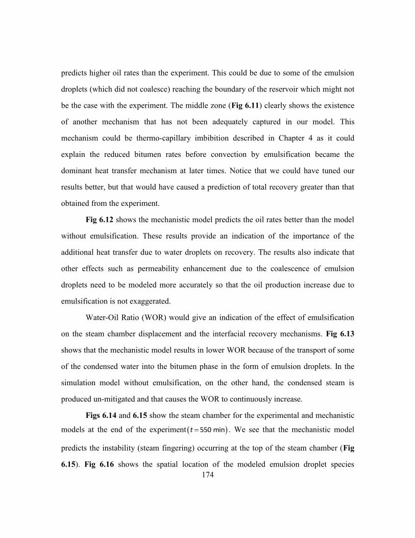
174
predicts higher oil rates than the experiment. This could be due to some of the emulsion
droplets (which did not coalesce) reaching the boundary of the reservoir which might not
be the case with the experiment. The middle zone (Fig 6.11) clearly shows the existence
of another mechanism that has not been adequately captured in our model. This
mechanism could be thermo-capillary imbibition described in Chapter 4 as it could
explain the reduced bitumen rates before convection by emulsification became the
dominant heat transfer mechanism at later times. Notice that we could have tuned our
results better, but that would have caused a prediction of total recovery greater than that
obtained from the experiment.
Fig 6.12 shows the mechanistic model predicts the oil rates better than the model
without emulsification. These results provide an indication of the importance of the
additional heat transfer due to water droplets on recovery. The results also indicate that
other effects such as permeability enhancement due to the coalescence of emulsion
droplets need to be modeled more accurately so that the oil production increase due to
emulsification is not exaggerated.
Water-Oil Ratio (WOR) would give an indication of the effect of emulsification
on the steam chamber displacement and the interfacial recovery mechanisms. Fig 6.13
shows that the mechanistic model results in lower WOR because of the transport of some
of the condensed water into the bitumen phase in the form of emulsion droplets. In the
simulation model without emulsification, on the other hand, the condensed steam is
produced un-mitigated and that causes the WOR to continuously increase.
Figs 6.14 and 6.15 show the steam chamber for the experimental and mechanistic
models at the end of the experiment 550 mint . We see that the mechanistic model
predicts the instability (steam fingering) occurring at the top of the steam chamber (Fig
6.15). Fig 6.16 shows the spatial location of the modeled emulsion droplet species

175
(EMULSO). These droplets are seen to largely exist at the steam chamber interface as
expected. This result is important because it signifies that the dispersion coefficients and
the degree of adsorption used to match recovery were just about right to prevent steam
from entraining the emulsion droplets and segregated flow of the emulsions in the oleic
phase due to gravity. Such flow of the emulsions mainly along the steam chamber
interface was also observed by Sasaki et al. (2002) in their experiments. The relatively
larger thickness of the steam chamber interface at the bottom than at the top (Fig 6.16)
suggests that emulsification tends to increase countercurrent flow (and hence, efficiency
of heat transfer) of steam and condensate/flowing bitumen along the steam chamber
walls. This must be caused by increased drag on the walls of the chamber due to the
downward flow of emulsion droplets by gravity.
The onset of emulsification is not expected to be uniform throughout the steam
chamber interface, and should in general be dependent on the magnitude of shear forces
acting at the interface. This needs to be further investigated.
Table 6.6 shows the important results of the tuned parameters, and we see that
each of them is physically realistic given the operating scale of the experiment. The
significance of each of these parameters will be discussed in a sensitivity study below.
In an attempt to understand why the presence of W/O emulsions improves heat
transfer at the steam chamber interface, we modeled a time snapshot of Sasaki et al.’s
(2001) experiment using COMSOLTM
Multiphysics. Fig 6.18 shows a COMSOLTM
Multiphysics simulation of the half chamber width where heat transfer has been coupled
with porous media fluid flow by gravity. We approximated the fluid distribution as that in
our simulations of Sasaki et al.’s (2001) experiment and introduced the emulsion droplets
as small liquid water spheres having the same temperature as steam. Fig 6.19 shows that
the effective heat transfer coefficient increases as the fractional volume of the emulsions

176
in the bitumen phase increases and reveals an almost two-fold increase from the case
without emulsions (i.e. at zero emulsion volume %). This is because the more the
volumes of emulsion droplets, the more is the convective heat transfer component. This
effect also plateaus at about 14% volume fraction and hence, there will exist an optimal
emulsion concentration for the purposes of improved heat transfer at the steam chamber
interface. Fig 6.20 shows that the effective heat transfer coefficient also increases as the
radius of the emulsion droplets increases and reveals an almost two-fold increase from
the case without emulsions for a given fractional volume of emulsion droplets. This is
because of increased surface area to heat transfer, thereby increasing heat transfer to the
bitumen phase. Figs 6.18 to 6.20 taken together explains why the presence of emulsion
droplets enhances SAGD rates as the effective heat transfer coefficient at the steam
chamber interface increases due to the presence of the emulsion droplets. This can also be
better understood from the context of Butler’s drainage equation (2.1) where a 100%
increase in the effective thermal diffusivity will trump any increase in the effective
viscosity of emulsified bitumen at steam temperature and the effective Butler m parameter
due to the presence of emulsion droplets in the bitumen phase.
Table 6.2: Properties of experimental sand pack (courtesy Sasaki et al. (2001a)
Parameter Values
Porosity, fraction 0.38
Average Permeability, K 1.42 x 10⁵mD
Thermal Conductivity, 0.7 J/cm.min.0C
Volumetric Heat Capacity 1.99 J/cm3.0C
Resin Thermal Conductivity 0.13 J/cm.min.0C
Resin Volumetric Heat Capacity 1.67 J/cm3.0C
Overall Heat Transfer Coefficient
from resin to surrounding air
0.041 J/cm2.min

177
Table 6.3: Bitumen properties (courtesy Sasaki et al. (2001a)
Parameter Values
Density 0.998 g/cm3
Molecular Weight 490 g/gmole
Compressibility 7.0 x 10⁻⁷ kPa-1
Thermal Expansion Coefficient 6.0 x 10⁻⁴ 0C-1
Heat Capacity 411.7 J/gmol 0C
Critical Pressure 1,115 kPa
Critical Temperature 4940C
Capillary Pressure 0.0 kPa
Phase Equilibrium Constant 0.0
Table 6.4: Bitumen viscosity (courtesy Sasaki et al. (2001a)
Temp. Viscosity Temp. Viscosity
0C cP
0C cP
15 15,000 65 996
20 9,200 75 624
25 6,913 85 418
35 4,015 95 286
45 2,412 105 200
55 1,495 120 60
Table 6.5: Initial conditions and saturation endpoints (courtesy Sasaki et al. (2001a)
Parameter Values
Temperature 20.0 0C
Pressure 101.3 kPa
Oil Saturation fraction 1.0
Water Saturation fraction 0.0
Gas Saturation fraction 0.0
Reference Pressure 101.3 kPa
Reference Temperature 20.0 0C
Sor fraction 0.05
Swc fraction 0.10
Sgc fraction 0.05

178
Table 6.6: Showing the final model results and tuned parameters
Parameter Tuned Values
Rate Constant, k 0.12 min-1
Reaction Order, 1
Dispersion coefficients, LD 1 cm2/min
Enthalpy of Emulsification, EMULSH 30 J/gmol
Figure 6.4: Linear relative permeability curves for sand pack model (used by Sasaki et
al. 2001a)

179
Figure 6.5: Modeling permeability enhancement to oil on coalescence of EMULSO
(Kovscek, 2009)
Figure 6.6: Comparison plot for cumulative oil recovery showing necessary fitting
values of permeability without emulsion modeling

180
Figure 6.7: Comparison plot for cumulative oil recovery showing necessary fitting
values of porosity without emulsion modeling
Figure 6.8: Comparison plot for cumulative oil recovery showing sensitivity to joint
porosity and permeability modeling using the Carman-Kozeny relation
without emulsion modeling

181
Figure 6.9: Comparison plot for cumulative oil recovery showing necessary fitting
values for overall heat transfer coefficient and resin thermal conductivity
without emulsion modeling
Figure 6.10: Comparison plot for cumulative oil recovery showing the sensitivity to the
relative permeability exponent without emulsion modeling
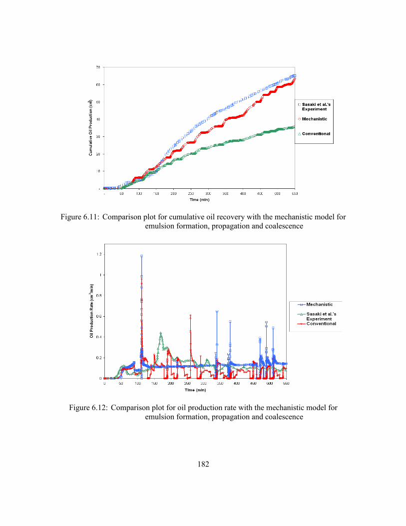
182
Figure 6.11: Comparison plot for cumulative oil recovery with the mechanistic model for
emulsion formation, propagation and coalescence
Figure 6.12: Comparison plot for oil production rate with the mechanistic model for
emulsion formation, propagation and coalescence

183
Figure 6.13: Comparison plot for water-oil-ratio (WOR) with the mechanistic model
Figure 6.14: Steam chamber for experimental model at 550mint (courtesy Sasaki et al.,
2001a) © 1996 Society of Petroleum Engineers
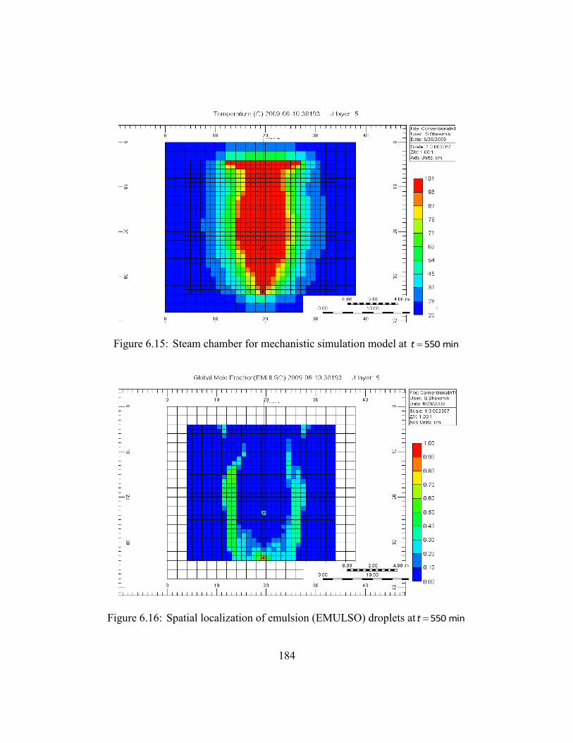
184
Figure 6.15: Steam chamber for mechanistic simulation model at 550 mint
Figure 6.16: Spatial localization of emulsion (EMULSO) droplets at 550 mint

185
Figure 6.17: Spatial localization of emulsion (EMULSO) droplets with dispersion
coefficient 20 cm minD at 550 mint
Figure 6.18: Half width of the steam chamber showing temperature (K) profiles using
COMSOLTM
Multiphysics
steam thermal
boundary layer condensate thermal
boundary layer
bitumen thermal
boundary layer
Ueff

186
Figure 6.19: Effective heat transfer coefficient (W/m-K) vs. volume % of emulsion
droplets for 0.05 mm droplets using COMSOLTM
Multiphysics
Figure 6.20: Effective heat transfer coefficient vs. radius of emulsion droplets for 12.27%
emulsion volume using COMSOLTM
Multiphysics
0
0.1
0.2
0.3
0.4
0.5
0.6
0.7
0 2 4 6 8 10 12 14
Vol. % of Emulsion droplets
Effe
ctiv
e H
eat T
rans
fer C
oeff.
droplet radius = 0.05mm

187
6.6.1 Sensitivity analysis
We investigated the sensitivity of the recovery to various fitting parameters. Such
analysis is necessary to expand our understanding of the emulsification process and to
streamline the scope of future research. In the following, we systematically and
independently varied all the fitting parameters. Stability was crucial in these simulations,
and a change in one parameter sometimes caused the simulator to report higher material
balance errors. In order to avoid this, we constrained our analysis only to results that
resulted in stable and accurate simulations.
Fig 6.21 shows a fairly uniform increase in recovery with a decrease in reaction
order. This increase is expected (concentration of EMULSW is always less than unity and
hence a decrease in reaction order will always lead to an increase in reaction rate) but its
uniformity indicates there is little resistance to spontaneous emulsification at the interface
of the steam chamber (i.e. mass transfer is playing an insignificant role in the kinetics of
emulsification for this system). Also, the uniformity can also mean that the reaction order
is dependent more on the properties of the reservoir and less on the properties of the fluid
that are changing with time. However, because the specification of chemical reaction is
only to mimic the physical process of emulsion formation, the sensitivity of the recovery
to various factors affecting viscous or density instability at the interface will be the
subject of future research.
Fig 6.23 shows an interesting feature – the possible existence of a threshold above
which emulsification disproportionately enhances recovery. Unlike the reaction order, the
rate constant and enthalpy of emulsification could be dependent more on the changing
fluid properties (steam and bitumen) than on the reservoir properties.
Fig 6.25 shows that recovery is enhanced when the emulsion droplets do not leave
the steam chamber interface by dispersion (corresponding to the case with dispersion

188
coefficient equal to zero). A plausible mechanism for this is steam entrainment of the
emulsion droplets. As injected steam rises to the top of the reservoir, it tends to entrain
lower energy state emulsion droplets, until such droplets attain sufficient energy
(determined by the dispersion coefficient) to break-through the interface of the steam
chamber. If this higher energy state is not achieved, rising steam then tends to spread the
droplets evenly inside the chamber which then increases the effective volume of cold
bitumen in contact with the hot emulsion droplets thereby enhancing recovery. Fig 6.17
shows such entrainment in action when there is no dispersion. We see the emulsion
droplets largely reside inside the steam chamber.
Fig 6.28 shows that an enthalpy of emulsification of 0 to 30 KJ/gmol could have
obtained the same match in Fig 6.11 and that there exists a threshold enthalpy value of 30
KJ/gmol for the emulsification process beyond which the emulsification reaction ceases
to be typical i.e. it ceases to be a good surrogate for the physical emulsification process
itself. This can be better understood when compared with the enthalpy of vaporization of
water which is 40.65 KJ/g-mol.
In all the sensitivities (Figs 6.22, 6.24, 6.27 and 6.30), we see that whenever
recovery is enhanced, the water-oil-ratio (WOR) is reduced which is consistent with the
flow behavior of water-in-oil (W/O) emulsions.

189
Figure 6.21: Sensitivity of cumulative oil recovery to the order of reaction.
Figure 6.22: Sensitivity of the water-oil ratio (WOR) to the order of reaction

190
Figure 6.23: Sensitivity of cumulative oil production to the reaction rate constant
Figure 6.24: Sensitivity of the water-oil ratio to the reaction rate constant

191
Figure 6.25: Sensitivity of the cumulative oil recovery to the dispersion coefficient of the
emulsion droplets in oil
Figure 6.26: Sensitivity of oil production rate to the dispersion coefficient of the
emulsion droplets in oil

192
Figure 6.27: Sensitivity of the water-oil ratio to the dispersion coefficient of the emulsion
droplets in oil
Figure 6.28: Sensitivity of the cumulative oil recovery to the enthalpy of emulsification

193
Figure 6.29: Sensitivity of the oil production rate to the enthalpy of emulsification
Figure 6.30: Sensitivity of the water-oil ratio to the enthalpy of emulsification

194
6.7 Summary and Significance of Work
An attempt has been made to model the effect of emulsion formation and
transport during the steam-assisted gravity drainage (SAGD) process on recovery. A
detailed framework, which involves process characterization using thirty-two (32) tuning
parameters, was developed. Model validation shows very promising results and indicates
that the emulsification process during SAGD might have a significant contribution
towards cumulative oil recovery.
The rate constant and reaction order dictate the speed or frequency of emulsion
generation at the interface of the steam chamber. However, the reaction order is expected
to be fairly constant if our assumption of an elementary reaction holds, and will be
dependent mainly on the properties of the reservoir. If this is the case, then for a given
reservoir, the rate constant will determine the frequency of emulsion generation, and will
be dependent on the properties of the heavy oil, steam temperature and pressure. The
dispersion coefficients determine the speed with which the emulsion droplets move
through (and leave) the steam chamber interface and hence heat transfer. The enthalpy of
emulsification represents instantaneous energy transferred to flowing bitumen close to the
interface. This is different from heat transferred by conduction and convection which are
time dependent. From our simulations, we observe that a typical range for EMULSH is 10
J/gmol to 30 KJ/gmol.
This work can be used to model improved recovery due to the presence of water-
in-oil (W/O) emulsions during SAGD at both the experimental and field scales. Field-
scale simulations will however require an effective scale-up process since the emulsion
droplets will be so much smaller than the average grid-block size.

195
Future experiments that make observations regarding the initiation of emulsion
formation as related to the steam chamber geometry and the heat transfer across the
steam-bitumen boundary will be invaluable. With these additional observations, a more
comprehensive theory for the formation and transport of W/O emulsions at the walls of
the steam chamber and the associated heat transfer mechanisms can be developed.

196
Chapter 7: Conclusions and Recommendations
In this chapter, we will summarize key conclusions and give recommendations for
future work.
7.1 Conclusions
In this work, we have studied improvements to the modeling of the SAGD
process by incorporating the effect of anisotropy, capillarity and W/O emulsification on
SAGD rates. We also extended the capillarity model to the ES-SAGD process. A central
insight from this work is that the SAGD process differs from most other enhanced oil
recovery (EOR) techniques in that it is a short length scale process and hence other short
length-scaled phenomena usually ignored in other EOR or conventional processes should
not be ignored for the SAGD process. We now present the key conclusions of this work
under these headings.
7.1.1 The Effect of Anisotropy
The effect of anisotropy on SAGD rates is time dependent generally obeying a
sigmoid or elliptic function. Since for anisotropic porous media, the directions of
resultant gravity head (RGH) and the resultant oil discharge (ROD) do not coincide, two
models describing anisotropy during SAGD was developed for both single layer and
multi-layered reservoirs.
The RGH and ROD models give similar results for 0.7v hk k but can give
dramatically different results for lower anisotropy ratios.

197
For multi-layered reservoirs, it is possible to define an equivalent anisotropy ratio,
but such equivalence does not apply to the ROD model.
We also showed that structured grid finite difference models might be unable to
predict accurately the effect of anisotropy due to the grid orientation effect and more
research still needs to be done to determine the more appropriate model between the
RGH and ROD models for the SAGD process.
This work will find invaluable use in well spacing design and in proxy models for
predicting the SAGD recovery.
7.1.2 The Effect of Heat Transfer on Capillarity during SAGD
Heat transfer plays an important role on capillary behavior during the SAGD
process. The existence of interfacial tension gradients due to temperature gradients ahead
of the steam chamber front creates the Marangoni effect of thermo-capillary imbibition of
the condensate into the bitumen phase.
This imbibition process is scale dependent and controlled by the Marangoni or
thermo-capillary number and explains why several models which do well at experimental
scales perform poorly at field scales and vice versa.
This work also shows that laboratory experiments used to predict field recovery
must be properly scaled to include, with the Butler scaling groups, all the dimensionless
groups developed in this work as phenomena completely absent at the experiment scale
can occur at the field scale for improperly scaled experiments.
This work will find strong application is scaled experiment design and improved
SAGD field scale recovery predictions.

198
7.1.3 The Effect of Heat Transfer on Capillarity during ES-SAGD
Heat transfer also plays a role in the capillary behavior of the ES-SAGD process.
Our model predicts that there exists a thermo-capillary number threshold below which
there is no benefit of the ES-SAGD process over SAGD.
Unlike for the SAGD process where heterogeneity is detrimental to SAGD rates
as more condensate will imbibe into the bitumen phase with increased heterogeneity,
heterogeneity has a more complex effect on ES-SAGD rates as it can also aid in the
transport of solvent farther away from the steam chamber interface thereby aiding
recovery.
An important result from this work is that it shows succinctly that the ratio of
solvent viscosity to bitumen viscosity at steam temperature also controls the additional
recovery from ES-SAGD over SAGD. If this ratio is close to unity, there is no benefit to
use the ES-SAGD process and the smaller this value is than unity, the better the
performance of the ES-SAGD process over SAGD. This is because the length scale of
both the SAGD and ES-SAGD processes are very short (effectively controlled by the
thermal conductivity and dispersive length scales), hence only the bitumen with
viscosities at temperatures close to the steam temperature will be contacted by the
solvent.
This work will also find strong application in scaled experiment design and
improved field scale recovery predictions and can be incorporated in a fast ES-SAGD
proxy for history matching, optimization and uncertainty analysis.
7.1.4 The Effect of Emulsion Formation and Transport during SAGD
The formation of water-in-oil (W/O) emulsions at the steam chamber interface
during SAGD enhances heat transfer during SAGD by inducing convective heat

199
transport. These W/O emulsions are hot water droplets dispersed into the bitumen phase
and help to enhance SAGD rates irrespective of the increased bitumen phase viscosity
due to the emulsion droplets because the effective heat transfer coefficient across the
steam chamber interface can effectively be doubled in the presence of W/O emulsions.
More work still needs to be done to determine if oil-in-water (O/W) emulsions
also form at the steam chamber interface during SAGD or if other complex combinations
do form. Also, it will be important to determine the incipient condition that triggers these
emulsions to form.
This work can be used to model improved recovery due to the presence of W/O
emulsions during SAGD at both experiment and field scales. Field-scale simulations will
however require an effective scale-up process since the emulsion droplets will be so
much smaller than the average grid-block size.
7.2 Recommendations for Future Work
This work can be extended further in a variety of ways, the most important being
the coupling of the three (3) phenomena studied. For example, the effect of capillarity can
be affected by anisotropy during SAGD since it will determine the effective permeability
used to define the thermo-capillary number. This effective permeability will be the
orthogonal components of the RGH and ROD models and given by equations (3.55) and
(3.56) respectively. Other couplings are also possible and should be explored.
We will now discuss individual possible extensions to this work under the natural
headings of this dissertation.

200
7.2.1 The Effect of Anisotropy
This wok did not fully resolve which of the RGH or the ROD models is best
suited for the SAGD process. Experimentation or Finite Element Method (FEM) based
numerical simulation should be used to explore this further.
We also only presented 2D models for the effect of anisotropy but most reservoirs
are 3D. It will be useful to extend our anisotropic models to 3D.
7.2.2 The Effect of Capillarity
We ignored the effect of wettability change in our model accounting for thermo-
capillary imbibition during SAGD. In reality, wettability also changes as interfacial
tension changes but probably not at the same time scale. Including the effect of
wettability might require either a transient extension of our model or it might be
illuminating to look at the “maximum” effect of wettability change by assuming it
changes at the same time scale as interfacial tension.
We extended the thermo-capillary model to the ES-SAGD process in this work,
but this can also be done to other solvent aided SAGD processes with some
modifications. For example, extensions to the lighter solvent aided processes like Steam
and Gas Push (SAGP) and Solvent alternating Solvent (SAS) processes will require the
additional use of gas/oil capillary pressure data since significant diffusion of the gas
phase occurs ahead of the steam chamber (Al-Murayri et al. 2011) and for the Amine-
Enhanced Steam-Assisted Gravity Drainage (AE-SAGD) process (Srivastava et al. 2010),
an additional constitutive equation relating the dependence of capillary pressure on amine
or surfactant concentration is needed.

201
7.2.3 The Effect of Emulsification
It is still not clear which emulsion type is predominantly produced during SAGD.
SAGD experiments seem to produce W/O emulsions while field scale recoveries seem to
produce O/W emulsions. This discrepancy seems to suggest that steam quality might be
playing an important role in the emulsification process since experiments are usually run
at high steam qualities while field scale recoveries will predominantly be operated at
lower steam qualities. More experiments will need to be performed to verify this.
In this dissertation, we assumed that emulsification is triggered at time 0t . This
might however not be the case as there will generally exist conditions that trigger the
emulsification process that would not have existed before steam injection. This will
require a combination of force balances across the steam chamber interface and some
instability analysis.
Extending the emulsion model we used in this work to field scales presents the
interesting challenge that the size of the average grid block for field scale simulations will
be far greater than the size of the emulsion droplets. Hence simulating the emulsion
problem at field scales will require some scale up process. A cohesive but novel theory
and method will be required for this.

202
Appendix A
We derive formally the resultant gravity head (RGH) and the resultant oil
discharge (ROD) models. Our derivations follow that of Das (2013) but with a SAGD
frame of reference.
From Fig 3.1, the oil velocities in the different directions can be written as
x h
hv k
x (A.1)
z v
hv k
z (A.2)
RGHRGH eff
RGH
hv k (A.3)
RODROD eff
ROD
hv k (A.4)
The velocity in the RGH direction can be decomposed further into
sin cosRGH z xv v v (A.5)
Substituting (A.1), (A.2) and (A.3) into (A.5) yields:
sin cos
RGHeff v h
RGH
h h hk k k
z x (A.6)
From geometry considerations

203
cos
RGH
h h
x (A.7)
and
sin
RGH
h h
z (A.8)
Substituting (A.7) and (A.8) into (A.6) yields:
2 2sin cosRGHeff v hk k k (A.9)
which is the required derivation for the RGH model. Similarly for the ROD model, an
effective gradient in the available head for discharge can be written as
sin cos
ROD
h h h
z x (A.10)
From (A.1), (A.2) and (A.4), we get
x
h
vh
x k (A.11)
z
v
vh
z k (A.12)
ROD
ROD
ROD eff
vh
k (A.13)

204
Also from geometry considerations, we get
cosx RODv v (A.14)
sinz RODv v (A.15)
Substituting equations (A.11) to (A.15) into (A.10) yields:
2 21 sin cos
RODeff v hk k k (A.16)
which is the required derivation for the ROD model.

205
Appendix B
B.1 Coordinate Transform
We consider the coordinate transformation from a fixed frame ,x y into a
moving frame , , attached to a moving front, as shown in Fig. B.1
Figure B.1: Fixed and moving coordinate systems
The moving coordinate system is chosen such that is the direction parallel to the front,
and the direction perpendicular to the front. It follows readily that:
1/22 2 cosfx x (B.1)
1/22 2 sinfy y (B.2)
where ,f fx y are the coordinates of the origin of the moving coordinate system, is the
angle between the direction and the y direction, and
arctan (B.3)
Using the trigonometric relations:
y
x xf
yf

206
cos cos cos sin sin (B.4)
sin sin cos cos sin (B.5)
(B.1) and (B.2) can be written as:
1 22 2 cos cos sin sinfx x (B.6)
1 22 2 sin cos cos sinfy y (B.7)
Using relation (B.3), it follows that:
1 2
cos (B.8)
1 2
sin (B.9)
Substituting (B.8) and (B.9) in (B.6) and (B.7) gives
cos sinfx x (B.10)
sin cosfy y (B.11)
which can be written in vector form as
1fx x R X (B.12)
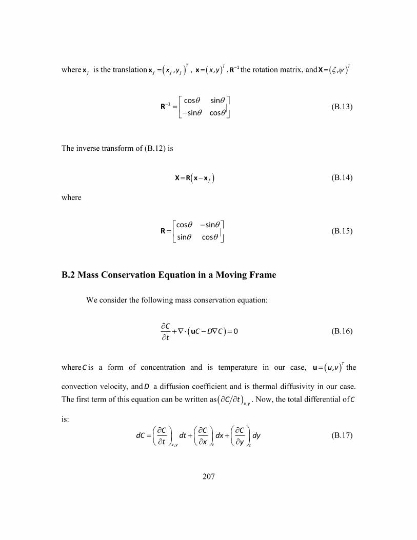
207
where fx is the translation ,T
f f fx yx , ,T
x yx , 1R the rotation matrix, and ,T
X
1cos sin
sin cosR (B.13)
The inverse transform of (B.12) is
fX R x x (B.14)
where
cos sin
sin cosR (B.15)
B.2 Mass Conservation Equation in a Moving Frame
We consider the following mass conservation equation:
0C
C D Ct
u (B.16)
whereC is a form of concentration and is temperature in our case, ,T
u vu the
convection velocity, and D a diffusion coefficient and is thermal diffusivity in our case.
The first term of this equation can be written as ,x y
C t . Now, the total differential ofC
is:
,x y t t
C C CdC dt dx dy
t x y (B.17)

208
Dividing by a time differential and taking and constant yields:
, , , ,x y t t
dC C C x C y
dt t x t y t (B.18)
Using equations (B.10) and (B.11) yields:
, ,
f f
x y t t
x ydC C C C
dt t x t y t (B.19)
Now, the total differential ofC is given by
, t t
C C CdC dt d d
t (B.20)
Dividing by a time differential and taking x and y constant yields:
, , , ,x y x y x yt t
C C C C
t t t t (B.21)
In vector form we can write:
, , ,x y x y
C CC
t t t
X (B.22)
where we have dropped the “constant-time” indication on C , defined as

209
,
T
t t
C CC (B.23)
Using equation (B.14), equation (B.23) can be written as:
, ,x y
C CC
t tU (B.24)
where
f
t
XU R (B.25)
is the velocity of the front, expressed in the directions and . The convection term of
(B.16) can be written as follows:
p pdx dyC C C
x dt y dtu (B.26)
where ,yp px is the position of a fluid particle in a moving coordinate system. Using
partial derivatives, with (B.12) and (B.14) yields:

210
cos sin cos
cos sin sin
sin cos sin
sin cos cos
p p
f
p p
f
p p
f
p p
f
d dC u C
dt dt
d du C
dt dt
d dv C
dt dt
d dv C
dt dt
u
(B.27)
The front velocities are by definition not a function of and , so that from (B.27) it
follows that
C Cu υ (B.28)
where andυ are respectively a space derivative operator and a fluid velocity in the
moving reference frame. It is also relatively straightforward to show that the diffusion
term is not affected by the coordinate transform, so that the conservation equation in the
moving system becomes:
0C
C C D Ct
U υ (B.29)

211
Appendix C
C.1 Experimental Modeling of the SAGD process
We present an experimental study of the SAGD process which was intended to be
used to study emulsification behavior during SAGD. As will be seen from the
temperature maps obtained during the experiment, we had trouble obtaining the classic
inverted triangle shape for the steam chamber that is central to the derivations for
recovery rate and steam chamber growth rate presented in this dissertation (and in
Butler’s work). Furthermore, our main motivation for performing the experiments was to
observe and measure any additional heat transfer that occurs at the steam-bitumen
interface due to the formation and transport of water-in-oil (W/O) emulsion droplets. The
measurement set up that we designed was insufficient to conclude that any enhanced heat
transfer occurs at the interface due to the transport of emulsion droplets. Given that the
results obtained by performing the experiments were inconclusive, we felt it best to
document the details of the experiments in this appendix rather than in the main body of
the dissertation.
The experimental setup is shown in Fig C.1 which follows a typical SAGD
process. Water is injected into an actuator through a pump to a steam generator which can
generate steam at varying qualities. A pressure transducer and solenoid valve is used to
prevent high pressures building up in the system and is connected to the reservoir (called
steam chamber in Fig C.1) which in turn is connected to a LabView 2009 Data
Acquisition System (DAQ) and an automatic fluid collection system that can be timed.
The DAQ was programmed to measure the temperature of the reservoir and the pressure
difference between the injector and producer. The reservoir has spacing for 100
thermocouples, but only 50 thermocouples were used in this experiment and ordinary

212
Kriging used to compute the temperatures of the remaining 50 unused thermocouple
locations.
C.1.2 Experimental Description
We describe each part of the experimental setup in this section. The reservoir is a
10in x 10in square model made of polycarbonate glass material. On the back is drilled
100 equally spaced thermocouple locations with design distances shown in Fig C.2. The
dimensions of the reservoir model are also shown in Fig C.2.
The fluid collection system is an automatic collector that can collect fluids at
timed intervals with a maximum time interval of 600 seconds. The DAQ is the main
electrical control for the experiment and is capable of recording temperature and pressure
data by converting voltage readings using a series of shunts and resistors. The pressure
transducer and solenoid valves are for steam pressure control. The polycarbonate glass
material is rated for 35psia and steam pressure is not allowed to rise above 20psia in our
experiments. This reduced the possible range of steam injection temperatures that could
be tested in the experiment.
The water tank or reservoir is used to store water required to produce steam, and
its volume was designed with the pump rate and expected duration of the experiment in
mind. After some iteration, the pump rate was kept constant at 10cc/min. The actuator
was used to connect the pump to the steam generator.
The steam generator used was capable of producing both saturated and
superheated steam. It had the capacity to run on 100% power or less. However, to ensure
only saturated steam is produced throughout the duration of the experiment for the given
operating pressure, a requisite steam generation power must be determined iteratively.

213
This is because back pressure effects causes superheated steam to be produced at higher
steam generation powers.
Figure C.1: Schematic of SAGD experimental model

214
Figure C.2: Schematic of the square reservoir model used for the experiment with some
important dimensions

215
C.1.2 Experimental Procedure
Each of the 50 thermocouples was first calibrated using a steam bath and at room
temperature. One of the thermocouples got damaged and we were hence left with only 49
thermocouples to work with. The pressure transducer was also calibrated using a
voltmeter. After calibration, the experimental setup was connected and ready for steam
injection.
Steam was injected into the reservoir at 10% power of the steam generator, after it
was determined that such power was sufficient to prevent the production of superheated
steam for about 5 hours of performing the experiment. The fluid collection system was
used to collect the produced fluids at varying intervals with the fluid rates obtained by
dividing the amount of fluid produced by the time interval at which it was produced. The
fluids produced were mostly in the form of oil-in-water (O/W) emulsions (probably
because we injected low quality steam) that could not easily be broken even with calcium
chloride de-emulsifying agent.
The temperatures in the steam chamber was recorded from the 49 thermocouples
by the DAQ and was interpolated to the entire reservoir by Ordinary Kriging using the
SGSIM geostatistical modeling software.
C.1.3 Experimental Results
The results from our experiment were mainly the temperature-time profiles and
are presented in Figs D.2 to D.11. They show the evolution of the steam chamber with
time through the temperature profile of the reservoir. Fig D.2, the initial condition of the
reservoir, shows some variation but this is clearly due to random noise either in the true
reservoir temperatures or in the thermocouple calibration process. True variations in
reservoir temperatures are seen with time and reveals that the steam chamber achieved

216
horizontal growth at about 30 minutes of steam injection. The growth of the steam
chamber is seen not to be uniform especially during its vertical growth and is a
consequence of microscopic heterogeneities inherent in the porous media packing
process.
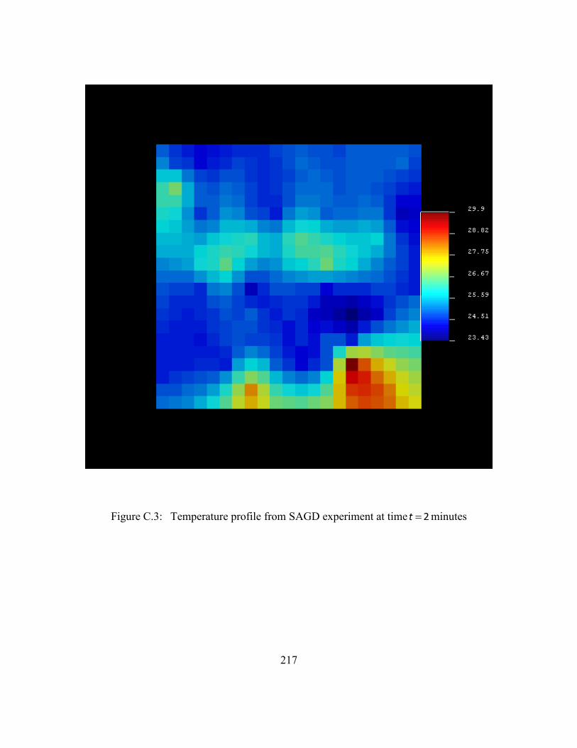
217
Figure C.3: Temperature profile from SAGD experiment at time 2t minutes

218
Figure C.4: Temperature profile from SAGD experiment at time 12t minutes

219
Figure C.5: Temperature profile from SAGD experiment at time 22t minutes

220
Figure C.6: Temperature profile from SAGD experiment at time 32t minutes

221
Figure C.7: Temperature profile from SAGD experiment at time 42t minutes

222
Figure C.8: Temperature profile from SAGD experiment at time 52t minutes

223
Figure C.9: Temperature profile from SAGD experiment at time 62t minutes

224
Figure C.10: Temperature profile from SAGD experiment at time 72t minutes

225
Figure C.11: Temperature profile from SAGD experiment at time 82t minutes

226
Figure C.12: Temperature profile from SAGD experiment at time 92t minutes

227
Figure C.13: Temperature profile from SAGD experiment at time 102t minutes

228
Figure C.14: Temperature profile from SAGD experiment at time 112t minutes

229
Bibliography
Aherne, A., Maini, B., 2008. Fluid Movement in the SAGD Process: A Review of the
Dover Project. Journal of Canadian Petroleum Technology 47 (1) Jan.
Akin, S., 2005. Mathematical Modeling of Steam-Assisted Gravity Drainage. SPE
Reservoir Evaluation & Engineering 8 (5) Oct.
Al-Bahlani, A.-M., Babadagli, T., 2009. SAGD laboratory experimental and numerical
simulation studies: A review of current status and future issues. Journal of
Petroleum Science and Engineering 68, 135–150.
Al-Murayri, M., Harding, T., Maini, B., 2011. Impact of Noncondensable Gas on
Performance of Steam-Assisted Gravity Drainage. Journal of Canadian Petroleum
Technology 50 (7) Jul.
Ananth Govind, P., Das, S., Srinivasan, S., Wheeler, T. J., 2008. Expanding Solvent
SAGD in Heavy Oil Reservoirs. Society of Petroleum Engineers, SPE 117571-
MS.
Arendo, V., Goulay, C., Stobie, G., Wall, T., Couput, J. P., 2005. The Challenges Facing
Multiphase Metering in Oil-Sands Thermal Developments. Society of Petroleum
Engineers, SPE 97751-MS.
Arya, Atul, Tom Hewett, Ronald Larson, and Larry Lake. 1988. “Dispersion and
Reservoir Heterogeneity.” SPE Reservoir Engineering 3 (1) (February).
Aster R. C., (2012), “Parameter Estimation and Inverse Problems”, 2nd edition,
Academic Press
Azad, A., 2012. Rapid SAGD Simulation Simulation Considering Geomechanics for
Closed Loop Reservoir Optimization, PhD Dissertation, University of Alberta,
Alberta, Canada.
Azad, A., Chalaturnyk, R., 2010. A Mathematical Improvement to SAGD Using
Geomechanical Modelling. Journal of Canadian Petroleum Technology 49 (10)
Oct.
Barillas, J.L.M., Dutra Jr., T.V., Mata, W., 2006. Reservoir and operational parameters
influence in SAGD process. Journal of Petroleum Science and Engineering 54,
34–42.

230
Beetge, J., 2005. Emulsion Stability Evaluation of SAGD Product with the IPR-CEF
Technique. Society of Petroleum Engineers, SPE 97785-MS.
Begg, S. H., and Chang, D. M., 1985. A Simple Statistical Method for Calculating the
Effective Vertical Permeability of a Reservoir Containing Discontinuous Shales.
Society of Petroleum Engineers SPE 14271-MS.
Bennison Trevor, 1998. Prediction of Heavy Oil Viscosity. Presented at the IBC Heavy
Oil Field Development Conference, London.
Birrell, G., 2003. Heat Transfer Ahead of a SAGD Steam Chamber: A Study of
Thermocouple Data From Phase B of the Underground Test Facility (Dover
Project). Journal of Canadian Petroleum Technology 42 (3) Mar.
Bogdanov, I. I., K. El Ganaoui, and A. M. Kamp. 2007. “COMSOL 2D Simulation of
Heavy Oil Recovery by Steam.” In COMSOL Users Conference. Grenoble:
COMSOL Multiphysics.
Bosch, R., Axcell, E., Little, V., Cleary, R., Wang, S., Gabel, R., Moreland, B., 2004. A
Novel Approach for Resolving Reverse Emulsions in SAGD Production Systems.
The Canadian Journal of Chemical Engineering 82, 836–839.
Bowman, C.W., 1967. Molecular and Interfacial Properties of Athabasca Tar Sands.
Presented at the 7th World Petroleum Congress, World Petroleum Congress,
Mexico City, Mexico.
Butler, R.M., Mcnab, G.S., Lo, H.Y., 1981. Theoretical studies on the gravity drainage of
heavy oil during in-situ steam heating. The Canadian Journal of Chemical
Engineering 59, 455–460.
Butler, R. M., and Stephens, D. J., 1981. The Gravity Drainage of Steam-heated Heavy
Oil to Parallel Horizontal Wells. Journal of Canadian Petroleum Technology, 90-
96, (April-June).
Butler, R., 1985. A New Approach To The Modelling of Steam-Assisted Gravity
Drainage. Journal of Canadian Petroleum Technology, 42-51, (May – June).
Butler, R., Mokrys, I., 1991. A New Process (VAPEX) For Recovering Heavy Oils Using
Hot Water And Hydrocarbon Vapour. Journal of Canadian Petroleum Technology
30 (1) Jan-Feb.
Butler, R. M. 1991. Thermal Recovery of Oil and Bitumen. Prentice Hall.
231
Butler, R. M., 1999. The Steam And Gas Push (SAGP). Journal of Canadian Petroleum
Technology 38 (3) Mar.
Butler, R.M., Dargie, B., CIM, P.S. of, 1994. Horizontal wells for the recovery of oil,
gas, and bitumen. Petroleum Society, Canadian Institute of Mining, Metallurgy &
Petroleum.
Castor, T.P., Somerton, W.H., 1977. Interfacial Instabilities in Porous Media. Society of
Petroleum Engineers, SPE 6516-MS.
Chalaturnyk, R., Li, P., 2004. When Is It Important to Consider Geomechanics in SAGD
Operations? Journal of Canadian Petroleum Technology 43 (4) Apr.
Chen, Q., Gerritsen, M., Kovscek, A., 2008. Effects of Reservoir Heterogeneities on the
Steam-Assisted Gravity-Drainage Process. SPE Reservoir Evaluation &
Engineering 11 (5) Oct.
Chung, K., Butler, R. M., 1988. Geometrical Effect of Steam Injection on The Formation
Of Emulsions In The Steam-Assisted Gravity Drainage Process. Journal of
Canadian Petroleum Technology 27 (1) Jan-Feb.
Chung, K., Butler, R. M., 1989. In Situ Emulsification By The Condensation Of Steam In
Contact With Bitumen. Journal of Canadian Petroleum Technology 28 (1) Jan-
Feb.
Chuoke, . L., Meurs, P. va., Van der Poel, C., 1959. The instability of slow, immiscible,
viscous liquid-liquid displacements in permeable media. AIME 216, 188–194.
Cuthiell, D., Green, K., Chow, R., Kissel, G., McCarthy, C., 1995. THE IN SITU
FORMATION OF HEAVY OIL EMULSIONS. Society of Petroleum Engineers,
SPE 30319-MS.
CMG. 2011. “CMG - STARS User Manual”. Computer Modeling Group.
Dalmazzone, C., Noïk, C., Glénat, P., Dang, H.-M., 2010. Development of a
Methodology for the Optimization of Dehydration of Extraheavy-Oil Emulsions.
SPE Journal 15 (3) Sep.
Das, Braja M. 2013. Advanced Soil Mechanics. 4th ed. Crc Pr I Llc.
Deutsch, C., 2010. Estimation of Vertical Permeability in the McMurray Formation.
Journal of Canadian Petroleum Technology 49 (12) Dec.

232
Donnelly, J., 1998. Who Invented Gravity? Journal of Canadian Petroleum Technology
37 (9) Sep.
Dykstra, H., Parsons, R.L., 1950. The Prediction of Oil Recovery by Waterflooding.
Secondary Recovery of oil in the United States 160–74.
Edmunds, Neil, and Simon Gittins. 1993. “Effective Application of Steam Assisted
Gravity Drainage of Bitumen to Long Horizontal Well Pairs.” Journal of
Canadian Petroleum Technology 32 (6) Jun.
Edmunds, N., 1999. On the Difficult Birth of SAGD. Journal of Canadian Petroleum
Technology 38 (1) Jan.
Einstein, A. 1906. Ann. Phys., Lpz., 19: 289.
Einstein. 1911. Ann. Phys., Lpz., 34: 591.
Ekwere J. Peters, 2012. Advanced Petrophysics: Volume 1: Geology, Porosity, Absolute
Permeability, Heterogeneity, and Geostatistics. Live Oak Book Company.
El-Khatib, Noaman. 1995. “Development of a Modified Capillary Pressure J-Function.”
SPE 29890-MS .
Eötvös, L. 1886. Annalen Der Physik 27: 448.
Farouq-Ali, S., 1997. Is There Life After SAGD? Journal of Canadian Petroleum
Technology 36 (6) Jun.
Flock, D. L., Le, T. H., Gibeau, J. P., 1986. The Effect Of Temperature On The
Interfacial Tension Of Heavy Crude Oils Using The Pendent Drop Apparatus.
Journal of Canadian Petroleum Technology, 25 (2) Mar-Apr.
Genuchten, Van, and M. Th. 1980. “A Closed-form Equation for Predicting the
Hydraulic Conductivity of Unsaturated Soils.” Soil Science Society of America
Journal 44 (5): 892–898.
Georgie, W., Smith, P.C., 2012. The Challenges in Processing Heavy Oil. Society of
Petroleum Engineers, SPE 157894-MS.
Gotawala, D.R., Gates, I.D., 2008. Steam fingering at the edge of a steam chamber in a
heavy oil reservoir. The Canadian Journal of Chemical Engineering 86, 1011–
1022.

233
Gupta, S. C., Gittins, S. D., 2006. Christina Lake Solvent Aided Process Pilot. Journal of
Canadian Petroleum Technology 45 (9) Sep.
Gupta, S., Gittins, S., 2012. An Investigation Into Optimal Solvent Use and the Nature of
Vapor/Liquid Interface in Solvent-Aided SAGD Process With a Semianalytical
Approach. SPE Journal 17 (4) Dec. (1255 - 1264)
Haldorsen, H., Lake, L., 1984. A New Approach to Shale Management in Field-Scale
Models. Society of Petroleum Engineers Journal 24 (4) Aug.
Harvey, Allan H. 1996. “Semiempirical Correlation for Henry’s Constants over Large
Temperature Ranges.” AIChE Journal 42 (5): 1491–1494.
Hornbrook, M.W., Dehghani, K., Qadeer, S., Ostermann, R.D., Ogbe, D.O., 1991. Effects
of CO2 Addition to Steam on Recovery of West Sak Crude Oil. SPE Reservoir
Engineering 6 (3) Aug.
Ito, Y., and T. Hirata. 1999. Numerical Simulation Study of a Well In the JACOS
Hangingstone Steam Pilot Project Near Fort McMurray. Journal of Canadian
Petroleum Technology 38 (13).
Ito, Y., and Suzuki, S., 1999. Numerical Simulation of the SAGD Process In the
Hangingstone Oil Sands Reservoir. Journal of Canadian Petroleum Technology
38 (9) Sep.
Javad S., P. Oskouei, B. Maini, R. Moore, and S. Mehta. 2010. Effect of Mobile Water-
Saturation on Thermal Efficiency of Steam-Assisted Gravity-Drainage Process.
SPE 138846-MS.
Kamath, V.A., Sinha, S., Hatzignatiou, D.G., 1993. Simulation Study of Steam-Assisted
Gravity Drainage Process in Ugnu Tar Sand Reservoir. Society of Petroleum
Engineers, SPE 26075-MS.
Kisman, K.E., Yeung, K.C., 1995. Numerical Study of the SAGD Process in the Burnt
Lake Oil Sands Lease. Society of Petroleum Engineers, SPE 30276-MS.
Kovscek, A. R. 2009. “Unlocking Heavy Oil and Unconventional Resources with Heat”
presented at the Petroleum & Geosystems Engineering Graduate Student Seminar
Series, April 27, The University of Texas at Austin.
Lake, L.W., 1996. Enhanced Oil Recovery, 1st ed. Prentice Hall.

234
Lantz, R.B. 1971. “Quantitative Evaluation of Numerical Diffusion (Truncation Error).”
Society of Petroleum Engineers Journal 11 (3) (September).
Le Ravalec, M., Morlot, C., Marmier, R., Foulon, D., 2009. Heterogeneity Impact on
SAGD Process Performance in Mobile Heavy Oil Reservoirs. Oil & Gas Science
and Technology - Revue de l’IFP 64, 469–476.
Leverett, M.C., 1941. Capillary behaviour in porous solids. Transactions of the AIME
142, 159–172.
Llaguno, P., Moreno, F., Garcia, R., Mendez, Z., Escobar, E., 2002. A Reservoir
Screening Methodology for SAGD Applications. Society of Petroleum Engineers.
Presented at the CIPC, Calgary, Alberta, June 11 - 13.
Lyford, Paul A., H.r.c Pratt, David C. Shallcross, and Franz Grieser. 1998. “The
Marangoni Effect and Enhanced Oil Recovery Part 1. Porous Media Studies.” The
Canadian Journal of Chemical Engineering 76 (2): 167–174.
Mandl, G., and C. W. Volek. 1969. “Heat and Mass Transport in Steam-Drive
Processes.” SPE Journal 9 (1): 59 – 79.
Marx, J. W., and R. H. Langenheim. 1959. “Reservoir Heating by Hot Fluid Injection.”
Petroleum Transactions AIME 216: 312–315.
McCormack, M., 2001. Mapping of the McMurray Formation for SAGD. Journal of
Canadian Petroleum Technology 40 (8) (August).
McLennan, J., Deutsch, C., Garner, D., Mus, E., Wheeler, T., Richy, J.-F., 2006.
Permeability Modeling for the SAGD Process Using Minimodels. Society of
Petroleum Engineers, SPE 103083-MS.
Mehdizadeh, P., 2005. High-Temperature Multiphase Flowmeters in Heavy-Oil Thermal
Production. Society of Petroleum Engineers, SPE 98009-MS.
Meyer, R. F., E. D. Attansasi, and P. A. Freeman. 2007. Heavy Oil and Natural Bitumen
Resources in Geological Basins of the World. Open File. US Geological Survey.
Mohammadzadeh, O., Rezaei, N., Chatzis, I., 2010. Pore-Level Investigation of Heavy
Oil and Bitumen Recovery Using Hybrid SAGD Process. Society of Petroleum
Engineers, SPE 130011-MS.
235
Najeh, A., Pishvaie, R. M., and Jabbari, H., 2009. A new semi-analytical modeling of
steam-assisted gravity drainage in heavy oil reservoirs. Journal of Petroleum
Science and Engineering 69, 261–270.
Nasr, T., S. Law, D., Golbeck, H., Korpany, G., 2000. Counter-current Aspect of the
SAGD Process. Journal of Canadian Petroleum Technology 39 (1) Jan.
Nasr, T., Beaulieu, G., Golbeck, H., Heck, G., 2003. Novel Expanding Solvent-SAGD
Process “ES-SAGD”. Journal of Canadian Petroleum Technology 42 (1) Jan.
Nasr, Tawfik, and Oluropo Ayodele. 2006. New Hybrid Steam-Solvent Processes for the
Recovery of Heavy Oil and Bitumen. In Society of Petroleum Engineers, SPE
101717-MS .
Nield, D.A., 1998. Modelling the Effect of Surface Tension on the Onset of Natural
Convection in a Saturated Porous Medium. Transport in Porous Media 31, 365–
368.
Noik, C., Dalmazzone, C., Goulay, C., Glenat, P., 2005. Characterisation and Emulsion
Behaviour of Athabasca Extra-Heavy-Oil Produced by SAGD. Society of
Petroleum Engineers, SPE 97748-MS.
Nukhaev, M., Pimenov, V., Shandrygin, A., Tertychnyi, V., 2006. A New Analytical
Model for the SAGD Production Phase. Society of Petroleum Engineers, SPE
102084-MS.
Oldroyd, J. G. 1953. “The Elastic and Viscous Properties of Emulsions and
Suspensions.” Proceedings of the Royal Society of London. Series A.
Mathematical and Physical Sciences 218 (1132) (June 9): 122–132.
Orr, Bryan. 2009. ES-SAGD; Past, Present and Future. In SPE Annual Technical
Conference and Exhibition. New Orleans, Louisiana, USA: SPE 129518-STU.
Peaceman, D.W., 1993. Reperesentation of a Horizontal Well in Numerical Reservoir
Simulation. SPE Advanced Technology Series 1 (1).
Plyasunov, Andrey V., and Everett L. Shock. 2003. “Prediction of the Vapor–liquid
Distribution Constants for Volatile Nonelectrolytes in Water up to Its Critical
Temperature.” Geochimica Et Cosmochimica Acta 67 (24) (December 15): 4981–
5009.

236
Rabiei Faradonbeh, M., Harding, T., Abedi, J., 2012. Semi-Analytical Modeling of
Steam-Solvent Gravity Drainage of Heavy Oil and Bitumen, Part 1: Enhanced
Flow Rate at Mobile Zone. Society of Petroleum Engineers, SPE 160316-MS.
Raghavan, R., and Marsden S.S. 1971a. “Theoretical Aspects of Emulsification in Porous
Media.” Society of Petroleum Engineers Journal 11 (2) (June).
Raghavan, R., Marsden, S.S., 1971b. The stability of immiscible liquid layers in a porous
medium. Journal of Fluid Mechanics 48, 143–159.
Raghavan, R., 1982. The Instability of Liquid-liquid Interfaces and Model Systems for
Emulsion Formation in Porous Media. University Microfilms.
Reis, J., 1992. A Steam-Assisted Gravity Drainage Model For Tar Sands: Linear
Geometry. Journal of Canadian Petroleum Technology 31 (10) Oct.
Reis, J., 1993. A Steam Assisted Gravity Drainage Model For Tar Sands: Radial
Geometry. Journal of Canadian Petroleum Technology 32 (8) Aug.
Sandler, Stanley I. 2006. Chemical, Biochemical, and Engineering Thermodynamics.
John Wiley & Sons.
Sanyi, W., Eric, A., Robert, C., Virgil, L., Lon, P., 2004. Application Of A Reverse-
Emulsion-Breaker At A SAGD Pilot Plant In Northern Alberta. Society of
Petroleum Engineers, SPE 86932-MS.
Sasaki, K., Akibayahsi, S., Yazawa, N., Doan, Q., Farouk Ali, S., 2001a. Numerical and
Experimental Modelling of the Steam Assisted Gravity Drainage (SAGD).
Journal of Canadian Petroleum Technology 40 (1) Jan.
Sasaki, K., Akibayashi, S., Yazawa, N., Doan, Q.T., Ali, S.M., 2001b. Experimental
Modeling of the SAGD Process - Enhancing SAGD Performance with Periodic
Stimulation of the Horizontal Producer. SPE Journal 6 (1) Mar.
Sasaki, K., Satoshi, A., Nintoku, Y., Fuminori, K., 2002. Microscopic Visualization with
High Resolution Optical-Fiber Scope at Steam Chamber Interface on Initial Stage
of SAGD Process. Society of Petroleum Engineers, SPE 75241-MS.
Serhat, A., Castanier, L., Brigham, W., 1999. Effect of Temperature on Heavy Oil/Water
Relative Permeabilities. Society of Petroleum Engineers, SPE 54120-MS.

237
Sharma, B., Santanu, K., Patil, S., Kamath, V., Dandekar, A., 2002. A Simulation Study
of Novel Thermal Recovery Methods in the Ugnu Tar Sand Reservoir, North
Slope, Alaska. Society of Petroleum Engineers, SPE 76729-MS.
Sharma, J., Gates, I., 2010a. Steam-Solvent Coupling at the Chamber Edge in an In Situ
Bitumen Recovery Process. Society of Petroleum Engineers, SPE 128045-MS.
Sharma, J., Gates, I.D., 2010b. Multiphase flow at the edge of a steam chamber. The
Canadian Journal of Chemical Engineering 88, 312–321.
Sharma, J., Gates, I., 2011. Convection at the Edge of a Steam-Assisted-Gravity-
Drainage Steam Chamber. SPE Journal 16 (3) Sep.
Sharma, J., Moore, R., Mehta, S., 2012. Effect of Methane Co-injection in SAGD −
Analytical and Simulation Study. Society of Petroleum Engineers Journal 17 (3)
Sep.
Shin, H., Choe, J., 2009. Shale Barrier Effects on the SAGD Performance. Society of
Petroleum Engineers, SPE 125211-MS.
Srivastava, Piyush, Vladimir Sadetsky, Justin Debord, Brian Stefan, and Bryan Orr. 2010.
Development of a Steam-Additive Technology To Enhance Thermal Recovery of
Heavy Oil. In Society of Petroleum Engineers, SPE 133465-MS.
Taylor, G. I. 1932. “The Viscosity of a Fluid Containing Small Drops of Another Fluid.”
Proceedings of the Royal Society of London. Series A 138 (834) (October 1): 41–
48.
Thimm, H. 2001. A General Theory of Gas Production in SAGD Operations. Journal of
Canadian Petroleum Technology 40 (11) Nov.
Thimm. 2006. Henry’s Law Near the Critical Point of Water-Applications in Solvent Co-
Injection With SAGD. Journal of Canadian Petroleum Technology 45 (1) Jan.
Torabzadey, S.J. and Handy L. L., 1984. The Effect of Temperature and Interfacial
Tension on Water/Oil Relative Permeabilities of Consolidated Sands. SPE 12689-
MS.
Veil, J. A., Quinn, J. J., 2008. Water Issues Associated with Heavy Oil Production.
Prepared of the U.S. Department of Energy, national Energy Technology
Laboratory.
238
Wagner, Wolfgang, and A. Pruss. 1993. “International Equations for the Saturation
Properties of Ordinary Water Substance. Revised According to the International
Temperature Scale of 1990. Addendum to J. Phys. Chem. Ref. Data 16, 893
(1987). Journal of Physical and Chemical Reference Data 22 (3): 783.
Wu, C.H., M.K. Beladi, G.P. Xue, M. Barrufet, I. Chawla, and K. Liu. 1997. Three Phase
K-Values of Heavy Paraffins and Crude Oil Pseudocomponents in Presence of
Water. In Society of Petroleum Engineers, SPE 37537-MS.
Xu, Yuming. 1990. Thermodynamic Investigations: 1. Gases and Vapours in Liquids; 2.
Calorimetric Studies. Ph.D., Alberta, Edmonton, AB: Alberta.
Yang, G., Butler, R. M., 1992. Effects of Reservoir Heterogeneities on Heavy Oil
Recovery by Steam-Assisted Gravity Drainage. Journal of Canadian Petroleum
Technology 31 (8) Aug.

239
Vita
Prince Nnamdi Azom was born in Nigeria and received his Bachelor of Science
degree in Chemical Engineering from the University of Lagos also in Nigeria, graduating
with a First Class (Hons.) in December 2006. He started his graduate studies at the
University of Texas at Austin in August 2007 and in May 2011, applied and obtained his
Master’s degree in Petroleum Engineering on his way to obtaining his PhD degree in the
same discipline. He had several internships during his graduate studies with Afren
Resources, USA and worked briefly as a Research Engineer at the Open & Experimental
Center for Heavy Oil (CHLOE), Pau, France in 2010. He is also the author of numerous
technical papers on modeling unconventional reservoirs. He is happily married with a son
and currently lives with his family in Alberta, Canada.
Permanent e-mail address: [email protected]
This thesis was typed by the author.