Maidan Summit 2011 - Harpreet Singh, Special Olympics Bharat (I)

Copyright
by
Harpreet Singh
2012

The Thesis Committee for Harpreet Singh
Certifies that this is the approved version of the following thesis:
Assessing Reservoir Performance and Modeling Risk Using Real
Options
APPROVED BY
SUPERVISING COMMITTEE:
Sanjay Srinivasan, Supervisor
Larry W. Lake
Supervisor:
Assessing Reservoir Performance and Modeling Risk Using Real
Options
by
Harpreet Singh, B.Tech
Thesis
Presented to the Faculty of the Graduate School of
The University of Texas at Austin
in Partial Fulfillment
of the Requirements
for the Degree of
Master of Science in Engineering
The University of Texas at Austin
May 2012

Dedication
This thesis is dedicated to my mother, and God.

v
Acknowledgements
I would like to express my sincere gratitude to my supervisor, Dr. Sanjay Srinivasan, for his
guidance, support, patience, and motivation throughout my master‟s studies at the University of
Texas at Austin. I am thankful to him for providing me the opportunity of pursuing my graduate
studies under his guidance. I am grateful to him for his good suggestions and wisdom on the
challenges that I faced outside my research. Without him, I would not have achieved this
milestone. I would also like to thank Dr. Larry Lake for reading this thesis and providing
valuable comments and suggestions.
I would like to thank my research group, especially Ankesh Anupam, Cesar Mantilla, and
Sayantan Bhowmik. I learned a lot from them. I am especially grateful to Ankesh Anupam for
being my unofficial research mentor. I am also thankful to the rest of my office mates and
friends, specifically, Brandon Henke, Namdi Azom, Selin Erzybek, Aarti Punase, Hoonyoung
Jeong, and Young Kim. Other past group members that I have had the great pleasure to work
with or alongside of are John Littlepage, Hapiz Zulkiply, Nader Bukhamseen, and Nitish
Koduru.
I would like to thank the friendly staff, each of whom helped in providing the resourceful
environment for the research. Specifically, Jin Lee for her help with the administrative support,
Dr. Roger Terzian for his help with the computer support, and all other staff members at the
Department of Petroleum and Geosystems Engineering. I would also like to thank CMG Ltd. for
providing me with full license of their simulator for the research.

vi
I would like to thank my mother, to whom I owe absolutely everything in life. Finally, I wish to
thank Garima Bajwa for her constant support and encouragement throughout this time.

vii
Abstract
Assessing Reservoir Performance and Modeling Risk Using Real Options
Harpreet Singh, M.S.E
The University of Texas at Austin, 2012
Supervisor: Sanjay Srinivasan
Reservoir economic performance is based upon future cash flows which can be generated from a
reservoir. Future cash flows are a function of hydrocarbon volumetric flow rates which a
reservoir can produce, and the market conditions. Both of these functions of future cash flows
are associated with uncertainties. There is uncertainty associated in estimates of future
hydrocarbon flow rates due to uncertainty in geological model, limited availability and type of
data, and the complexities involved in the reservoir modeling process. The second source of
uncertainty associated with future cash flows come from changing oil prices, rate of return etc.,
which are all functions of market dynamics. Robust integration of these two sources of
uncertainty, i.e. future hydrocarbon flow rates and market dynamics, in a model to predict cash
flows from a reservoir is an essential part of risk assessment, but a difficult task. Current
practices to assess a reservoir’s economic performance by using Deterministic Cash Flow (DCF)
methods have been unsuccessful in their predictions because of lack in parametric capability to
robustly and completely incorporate these both types of uncertainties.

viii
This thesis presents a procedure which accounts for uncertainty in hydrocarbon production
forecasts due to incomplete geologic information, and a novel real options methodology to assess
the project economics for upstream petroleum industry. The modeling approach entails
determining future hydrocarbon production rates due to incomplete geologic information with
and without secondary information. The price of hydrocarbons is modeled separately, and the
costs to produce them are determined based on market dynamics. A real options methodology is
used to assess the effective cash flows from the reservoir, and hence, to determine the project
economics. This methodology associates realistic probabilities, which are quantified using the
method’s parameters, with benefits and costs. The results from this methodology are compared
against the results from DCF methodology to examine if the real options methodology can
identify some hidden potential of a reservoir’s performance which DCF might not be able to
uncover. This methodology is then applied to various case studies and strategies for planning and
decision making.
ix
Table of Contents
Table of Contents ................................................................................................... ix
List of Tables ........................................................................................................ xii
List of Figures ...................................................................................................... xiii
Chapter 1: Introduction ............................................................................................1
Motivation .......................................................................................................1
Uncertainties In Upstream Petroleum Industry Projects .................................2
Thesis Outline .................................................................................................3
Chapter 2: Real Options ...........................................................................................5
Introduction .....................................................................................................5
Discounted Cash Flow ....................................................................................5
Real Options Valuation ...................................................................................6
DCF vs. ROV ..................................................................................................7
Black-Scholes Equation ..................................................................................7
Chapter 3: Model Updating and Value of Information ..........................................18
Introduction ...................................................................................................18
Research Approach .......................................................................................19
Incorporating Reservoir Uncertainty In ROV...............................................19
Assessing The Value Of Information ...........................................................22
Static Reservoir Modeling ............................................................................23
Flow Modeling ..............................................................................................31
ROV Analysis ...............................................................................................36
Results And Discussions ...............................................................................39
Chapter 4: Assessing Economic Implications of Reservoir Modeling Decisions .42
Introduction ...................................................................................................42
Assessing The Impact Of Detailed Geological Modeling ............................43
Assessing The Impact Of Detailed Flow Modeling ......................................69

x
Chapter 5: Binomial-Lattice Option Valuation......................................................77
Introduction ...................................................................................................77
Use Of The Model ........................................................................................78
Method For Constructing The Lattice...........................................................80
Relationship Of BLOV With Black-Scholes Model For ROV .....................86
Chapter 6: Analyzing the Prospects of an Undeveloped Field ..............................88
Introduction ...................................................................................................88
Description of the problem ...........................................................................89
Modeling Approach ......................................................................................89
Static Reservoir Modeling ............................................................................91
NPV Distribution Forecast ............................................................................94
Option Valuation By BLOV .........................................................................97
Results And Discussions .............................................................................101
Chapter 7: Uncertainty Analysis by Model Selection and Economic Evaluation Using a Binomial Lattice..........................................................................................106
Introduction .................................................................................................106
Model Selection Algorithm.........................................................................106
Case Description .........................................................................................108
Static Reservoir Modeling ..........................................................................109
Well History ................................................................................................115
Final Set of Models by Model Selection Algorithm ...................................117
Results .........................................................................................................119
Discussions .................................................................................................128
Chapter 8: Summary, Conclusions, and Future Recommendations ....................130
summary ......................................................................................................130
conclusions ..................................................................................................131
recommendations for future work ...............................................................132
Appendix A: Simulation Data Files for CMG-IMEX ..........................................134
A.1 Reservoir Model: 50 x 50 x 1Grid Dimension, 5 Production Wells (Chapter 3) 134
xi
A.2 Reservoir Model: 200 x 200 x 1Grid Dimension, 5 Production Wells (Chapter 4)............................................................................................................142
A.3 Reservoir Model: 200 x 200 x 1Grid Dimension, 5 Production Wells, Well testing (Chapter 7) .........................................................................................151
Appendix B: MatLab Codes to Perform General Operations ..............................168
B.1 Importing Data From GSLIB Format Files To MatLab .......................168
B.2 Making a Data File With GSLIB Format From MatLab Workspace ..169
B.3 Calling CMG-IMEX From Matlab To Retrieve Bottom Hole Pressure (BHP) Data............................................................................................................171
B.4 Calling CMG-IMEX From Matlab To Retrieve Production Rate Data174
B.5 Computing Production Rate Through Decline Curve Analysis ...........177
B.6 PV, NPV And ROV Analysis ..............................................................180
B.7 NPV And Reserve Estimation By STOOIP .........................................185
B.8 BLOV Anlysis ......................................................................................188
B.9 Calling GSLIB Executable „TRANS‟ From MatLab And Retrieving The Resultant Data ....................................................................................................193
B.10 Generating Sample Data And Their Co-Ordinates From A Gridded Data 195
B.11 Computing Permeability By Drawdown/Buildup Well Testing Data 198
Appendix C: MatLab Codes for Specific Cases and Chapters ............................209
C.1 Model Updating And Value Of Information (Chapter 3) ....................209
C.2 Assessing Economic Implications of Reservoir Modeling Decisions (Chapter 4) 217
C.3 Analyzing the Prospects of an Undeveloped Field (Chapter 6) ...........224
C.4 Analyzing Reservoir Performance by Model Selection (Chapter 7)....229
Bibliography ........................................................................................................239

xii
List of Tables
Table 3-1: Hard (core) data of porosity and permeability obtained at the 5 producing well locations ........................................................................................................................................ 23 Table 3-2: Hard data of porosity and permeability after drilling an additional well (in yellow) . 26 Table 4-1: Hard data of porosity and permeability from 5 reference wells .................................. 45 Table 4-2: Conditioning data at well locations in form of two facies .......................................... 51 Table 6-1: Hard data of porosity from 5 wells and their locations ............................................... 91 Table 7-1: Hard data of porosity and permeability from 5 reference wells ................................ 110 Table 7-2: Threshold values of permeability and porosity with their corresponding marginal probabilities................................................................................................................................. 113 Table 7-3: Locations of 5 wells .................................................................................................. 115
xiii
List of Figures
Figure 3-1: Algorithm for incorporating reservoir uncertainty in ROV ....................................... 21 Figure 3-2: Porosity (%) and permeability (md) model on left and right, respectively, for the base case ................................................................................................................................................ 25 Figure 3-3: Two realizations of each porosity (left side; in %) and permeability (right side; in md), respectively, after drilling an exploratory well (green colored circle) ................................. 28 Figure 3-4: a) Secondary data mimicking seismic; b) Two realizations of each porosity (%) and permeability (md) model on left and right, respectively, after acquiring seismic ........................ 30 Figure 3-5: Two phase relative permeability curve for oil-water phase ....................................... 32 Figure 3-6: Reservoir model setup in CMG for simulations ........................................................ 33 Figure 3-7: Uncertainty in production rate profiles for a) base case, b) after an exploratory well, c) after seismic .............................................................................................................................. 34 Figure 3-8: Change in uncertainty of oil production forecast after obtaining information from drilling an exploratory well. .......................................................................................................... 35 Figure 3-9: Change in uncertainty of oil production forecast after conditioning to secondary data mimicking seismic. ....................................................................................................................... 35 Figure 3-10: Change in uncertainty of oil production forecast ..................................................... 36 Figure 3-11: Variation of project volatility with time during the life of the reservoir ................. 38 Figure 3-12: Comparison of uncertainty in cumulative DCF for scenarios 1 and 2 with base case....................................................................................................................................................... 39 Figure 3-13: Uncertainty in ROV due to uncertainty in production forecasts .............................. 40 Figure 3-14: Uncertainty in PV due to uncertainty in production forecasts ................................. 40 Figure 4-1: Reference Model for porosity (left; in %) and permeability (right; in md) ............... 46 Figure 4-2: Isotropic model fit (black) for experimental semivariograms (red) of porosity in four directions ....................................................................................................................................... 47 Figure 4-3: Isotropic model fit (black) for experimental semivariograms (red) of permeability in various directions .......................................................................................................................... 48 Figure 4-4: Maps from SGSIM ..................................................................................................... 50 Figure 4-5: Maps from SISIM ...................................................................................................... 51 Figure 4-6: TI used as input in the SNESIM program .................................................................. 52 Figure 4-7: Maps from SNESIM .................................................................................................. 53 Figure 4-8: Average of SGSIM (top), SISIM (middle) and SNESIM (bottom) maps over the suite of 100 realizations ......................................................................................................................... 54 Figure 4-9: Two phase oil-water relative permeability curve assumed for the flow simulations . 56 Figure 4-10: Reservoir model setup in CMG for simulations ...................................................... 57 Figure 4-11: Uncertainty in oil production forecast obtained using SGSIM ................................ 58 Figure 4-12: Uncertainty in oil production forecast obtained using SISIM ................................. 58 Figure 4-13: Uncertainty in oil production forecast obtained using SNESIM ............................. 59 Figure 4-14: Comparison of production rate distributions (histograms) from 3 geological models with the reference truth ................................................................................................................. 60 Figure 4-15: Variation of project volatility with time for different models and reference truth .. 62 Figure 4-16: Comparison of uncertainty in cumulative DCF from SGISIM, SISIM, and SNESIM with that ........................................................................................................................................ 63

xiv
Figure 4-17: Uncertainty in PV forecast obtained using SGSIM ................................................. 64 Figure 4-18: Uncertainty in PV forecast obtained using SISIM ................................................... 65 Figure 4-19: Uncertainty in PV forecast obtained using SNESIM ............................................... 65 Figure 4-20: Uncertainty in ROV forecast obtained using SGSIM .............................................. 66 Figure 4-21: Uncertainty in ROV forecast obtained using SISIM ............................................... 66 Figure 4-22: Uncertainty in ROV forecast obtained using SNESIM ........................................... 67 Figure 4-23: Comparison of mean production profiles from different models ............................ 68 Figure 4-24: Comparison of ROV corresponding to mean production profiles from different models ........................................................................................................................................... 68 Figure 4-25: Uncertainty in oil production forecast determined using CMG ............................... 73 Figure 4-26: Uncertainty in oil production forecast determined using decline curve analysis .... 73 Figure 4-27: Uncertainty in PV obtained using CMG .................................................................. 74 Figure 4-28: Uncertainty in PV obtained using Decline Curve .................................................... 74 Figure 4-29: ROV obtained using CMG ....................................................................................... 75 Figure 4-30: ROV obtained using Decline Curve ......................................................................... 75 Figure 5-1: Example of a lattice showing underlying asset values ............................................... 79 Figure 5-2: Example of a lattice showing option values ............................................................... 79 Figure 5-3: Construction of lattice for an underlying asset illustrating the process of construction of lattice for an underlying asset. The value of the asset is first constructed by going from left to right. Subsequently, the option value is computed by traversing the lattice from right to left. .... 81 Figure 5-4: Probability distribution of future payoffs obtained from the values in the terminal nodes of the underlying lattice ...................................................................................................... 82 Figure 5-5: Construction of Option Valuation Lattice .................................................................. 85 Figure 5-6: Evolution of Option Valuation Lattice....................................................................... 86 Figure 6-1: Porosity with reference data only ............................................................................... 92 Figure 6-2: Seismic map on a 50 x 50 x 1 grid scale .................................................................... 93 Figure 6-3: Porosity with reference data and seismic ................................................................... 94 Figure 6-4: Distribution of NPV values for a) Scenario 1. The reservoir models have been generated conditioned to only 5 well data; b) Scenario 2. The reservoir models have been generated conditioned to 5 well data and the pseudo-seismic data .............................................. 95 Figure 6-5: P10, P25, P50, P75, and P90 values retrieved from the NPV distribution for Scenario 1 and Scenario 2. ........................................................................................................................... 96 Figure 6-6: a) Illustration for constructing lattice of the underlying asset; b) Calculation of underlying asset value using 5 well data for 1 time step. ............................................................. 98 Figure 6-7: a) Illustration for constructing option valuation lattice; b) Calculation of option valuation lattice using 5 well data for 1 time step. ....................................................................... 99 Figure 6-8: Lattice of the underlying asset with reference data only ......................................... 101 Figure 6-9: Option valuation lattice with reference data only .................................................... 102 Figure 6-10: Lattice of the underlying asset with reference data and seismic ............................ 102 Figure 6-11: Option valuation lattice with reference data and seismic ...................................... 103 Figure 6-12: Uncertainty in option values generated using P-values of the NPV ...................... 104 Figure 7-1: Algorithm for model selection by distance-metric approach ................................... 108 Figure 7-2: Isotropic model fit (black) for experimental variograms (red) of porosity in various directions ..................................................................................................................................... 111
xv
Figure 7-3: Isotropic model fit (black) for experimental variograms (red) of permeability in various directions ........................................................................................................................ 112 Figure 7-4: Single realization for each porosity (%) and permeability (md) .............................. 114 Figure 7-5: Multiple realizations of permeability field ............................................................... 114 Figure 7-6: Reservoir model setup in CMG for flow simulation................................................ 115 Figure 7-7: Well bottom hole pressure during drawdown and buildup well test for well-1 ....... 116 Figure 7-8: Well bottom hole pressure during drawdown and buildup well test for well-2 ....... 117 Figure 7-9: Uncertainty in oil flow rates from the reservoir before and after model selection .. 118 Figure 7-10: NPV distribution before model selection ............................................................... 120 Figure 7-11: Key percentile values of the NPV distribution before model selection ................. 121 Figure 7-12: NPV distribution after the model selection ............................................................ 122 Figure 7-13: Key percentiles of the NPV distribution after the model selection........................ 122 Figure 7-14: Variation of project volatility with time for models before and after selection, and reference truth ............................................................................................................................. 124 Figure 7-15: Underlying lattice of the reference truth model ..................................................... 125 Figure 7-16: Option lattice of the reference truth model ............................................................ 126 Figure 7-17: Underlying lattice before the model selection ....................................................... 126 Figure 7-18: Option lattice before the model selection .............................................................. 127 Figure 7-19: Underlying lattice after the model selection .......................................................... 127 Figure 7-20: Option lattice after the model selection ................................................................. 128 Figure 7-21: Uncertainty in option values generated using P-values of the NPV ..................... 129

1
Chapter 1: Introduction
MOTIVATION
Project evaluation under uncertainty is a key aspect of reservoir engineering and management
that has assumed a critical role in recent times because of the depletion of easy to produce
hydrocarbon resources and the increasing hostile operating environments faced by oil and gas
operators. However, there is a significant gap between theory as developed in academic literature
and the practical manner in which project evaluation is carried out in the industry. There is also a
gap in the way uncertainty is assessed using modern reservoir modeling tools and the
assumptions employed in economic tools for project evaluation. In light of the geological,
technical, economical and political uncertainties that confront major projects – flexibility in
making development decisions is essential. Thus we need options to change the capacity of
facilities, the scale of a project, the timing of investment etc. and these options must be evaluated
under technical and market uncertainties.
These motivate the use of real options valuation (ROV) for strategic planning and decision-
making. ROV is a technique that provides flexibility for including any changes that may be
associated with a project. Standard implementations of ROV for petroleum projects reveal a
distinct gap between the technologies for uncertainty assessment available within reservoir
modeling workflows and the representation of uncertainty in typical options evaluation. The
objective of this thesis is to expose some of these gaps and subsequently suggest a new workflow
for incorporating reservoir uncertainties in ROV analysis. The research also sheds some light on
2
issues such as optimum resolution of reservoir models, the level of detail in flow modeling etc.
as viewed from the standpoint of ROV analysis.
UNCERTAINTIES IN UPSTREAM PETROLEUM INDUSTRY PROJECTS
Decisions to invest in projects related to upstream petroleum engineering are made in the
presence of multiple sources of uncertainty. These decisions are based on future economic value
as determined by forecasting future hydrocarbon production from the reservoir, the cost
associated with production of those hydrocarbons, and the forecast of oil price prevailing during
the time period of hydrocarbon production.
Some of the uncertainties associated with valuing an upstream project are (Lin 2008):
1. Subsurface Uncertainty:
a. Geologic uncertainty - Uncertainty in predicting porosity, permeability, shape of
reservoir, fault structures etc.
b. Flow related uncertainty - Can include uncertainty in fluid properties, uncertainty
in reservoir drive mechanisms, uncertainty in sweep efficiency etc.
2. Surface Uncertainty: This type of uncertainty may include shut in of the well due to
changes in operating conditions such as weather (in case of offshore fields), failure in
operation of surface facilities etc.
3. Cost Uncertainty: This includes uncertainty in capital costs, operational costs etc.
4. Market Uncertainty: Such as changes in oil and gas prices, interest rates etc.
3
Although in reality, these uncertainties may exhibit coupled behavior rendering the analysis very
difficult, in this thesis, the focus is on geologic uncertainty and its manifestation in the ROV
analysis.
THESIS OUTLINE
The general research questions addressed in this thesis are:
1. How do we integrate geological uncertainty obtained by reservoir modeling within the
ROV framework?
2. How can we use ROV analysis to address important modeling issues such as optimal
representation of geology in reservoir models and the role of complex flow models for
uncertainty assessment?
3. What is the economic worth of incremental data for reservoir modeling?
Chapter 2 presents a review of real option valuation using the Black-Scholes model, and the
concepts associated with its application to projects in the upstream petroleum industry. This
concept will be used subsequently to value projects under geologic uncertainty. Chapter 3
presents a strategy for updating reservoir models as new information becomes available. The
economic forecasts of the project after integrating two sources of information are compared
using both deterministic cash flow technique and real options Black-Scholes model. Comparison
of results from both these techniques suggest that project valuation by the Black-Scholes model
results in a more robust assessment of the worth of additional data. Chapter 4 explores and
compares reservoir performance obtained by complex reservoir modeling (geological model and
reservoir simulation) and simple reservoir modeling for valuing long term E&P projects. Chapter
5 extends the real option valuation technique using Binomial Lattice, and the concepts associated
with its application to projects in upstream petroleum industry. Chapter 6 applies the framework

4
of Binomial Lattice Option Valuation (BLOV) to analyze the economic prospects of an
undeveloped, but discovered field. Chapter 7 proposes a strategy to save computational time for
doing uncertainty analysis, in context of reservoir performance and risk assessment, by
employing the use of model selection algorithm. The final chapter outlines conclusions and
presents recommendations for future work.

5
Chapter 2: Real Options
INTRODUCTION
An option is a form of contract between two members for future commercial transaction. An
important aspect of an option is that it is essentially a member‟s right, but not an obligation, to
form a contract with another member. A real option is an analogy of the financial options
applicable to projects and activities outside the stock market. A real option allows forming a
contract for future transactions in physical/real assets. Typically, this could be the option to
develop, abandon, expand etc. a capital intensive project. Another difference between financial
and real options is the time to expiration, which is the date on which the contract expires, and
after which the option becomes worthless. In financial options the date of expiration typically
ranges from one to two quarters, whereas in real options the date of expiration ranges in several
years.
Before embarking on a review of real option valuation, a brief look at a more traditional
approach to economic analysis is warranted.
DISCOUNTED CASH FLOW
Discounted Cash Flow (DCF) is a technique to value a project using the concept of time value of
money. In this technique, future cash flows are determined and discounted to obtain Present
Values (PV), and the sum of all PVs is the Net Present Value (NPV). NPV assumes all the risks
in a project are completely accounted for by the rate of return (r), and it does not allow for
uncertainty, changing circumstances etc.
6
( )
(1 )
Where,
( ) futurecash flow at time t
rateof return
t
F tNPV Benefits Costs
r
F t
r
REAL OPTIONS VALUATION
Real Options Valuation (ROV) is also a form of project valuation technique, but more advanced
than DCF. ROV is a process of valuing a physical/real asset with real uncertainties. As opposed
to NPV, ROV incorporates multi-domain uncertainties. Simply put, ROV is an extension to Net
Present Value (NPV)/Present Value (PV) analysis:
/ - NPV PV Benefits Cost
( ) - ( ) ROV Benefits P x Cost P y
Where, ( )P y represents the probability that the option will be positive (i.e. the benefit is greater
than the cost). If the option has been exercised (i.e. the costs have been incurred and cannot be
recovered), ( )P x represents the probability that subsequent benefits are also positive. Here x and
y are the variables through which these probabilities are quantified. It is evident from the above
equation that a major difference between the the NPV/PV evaluation and the ROV evaluation is
the introduction of uncertainty in current and future benefits through the probabilities ( )P . The
ROV can be estimated through a closed-form equation known as Black-Scholes equation. The
variables x and y will be defined in the upcoming section on Black-Scholes equation.

7
DCF VS. ROV
The focus of this chapter is on the concept of ROV, and the focus in the next two chapters is on
the application of ROV to evaluate models for geologic uncertainty, data integration etc. In order
to assess why ROV may be more realistic and flexible in valuing assets compared to NPV, here
are two reasons (Johnson 2010) that may specifically apply to petroleum E&P industry:
1. When an investment is valued using NPV, it is assumed that production rates are fixed
and there is no allowance for changes in future production rates that might occur due to
changing circumstances. However, as opposed to NPV, the ROV concept allows for
changing circumstances and in considering changes in future production rates.
2. The ability of ROV make use of more available information such as project volatility
due to oil price fluctuations as well as geologic uncertainty, schedule uncertainty etc.
DCF is still the basis to appraise potential investments for most oil companies. It is easy and
requires less information to appraise the valuation. It is believed (Coy 1999) that ROV yields
more realistic asset evaluation than DCF because the ROV model incorporates the variability and
uncertainty in the model parameters. ROV may highlight extra value for projects, where DCF
fails to see the hidden value, or may highlight low value of falsely bloated value projects by DCF
(Bailey et al. 2003). The strength of ROV is based on the accuracy of the parameters used in its
models and parameter selection is a vital part of ROV (Bailey et al. 2003).
BLACK-SCHOLES EQUATION
There are various derivations of the Black-Scholes equation. However, we present here the
derivation that invokes the usage of a formula in stochastic calculus known as Ito‟s lemma.
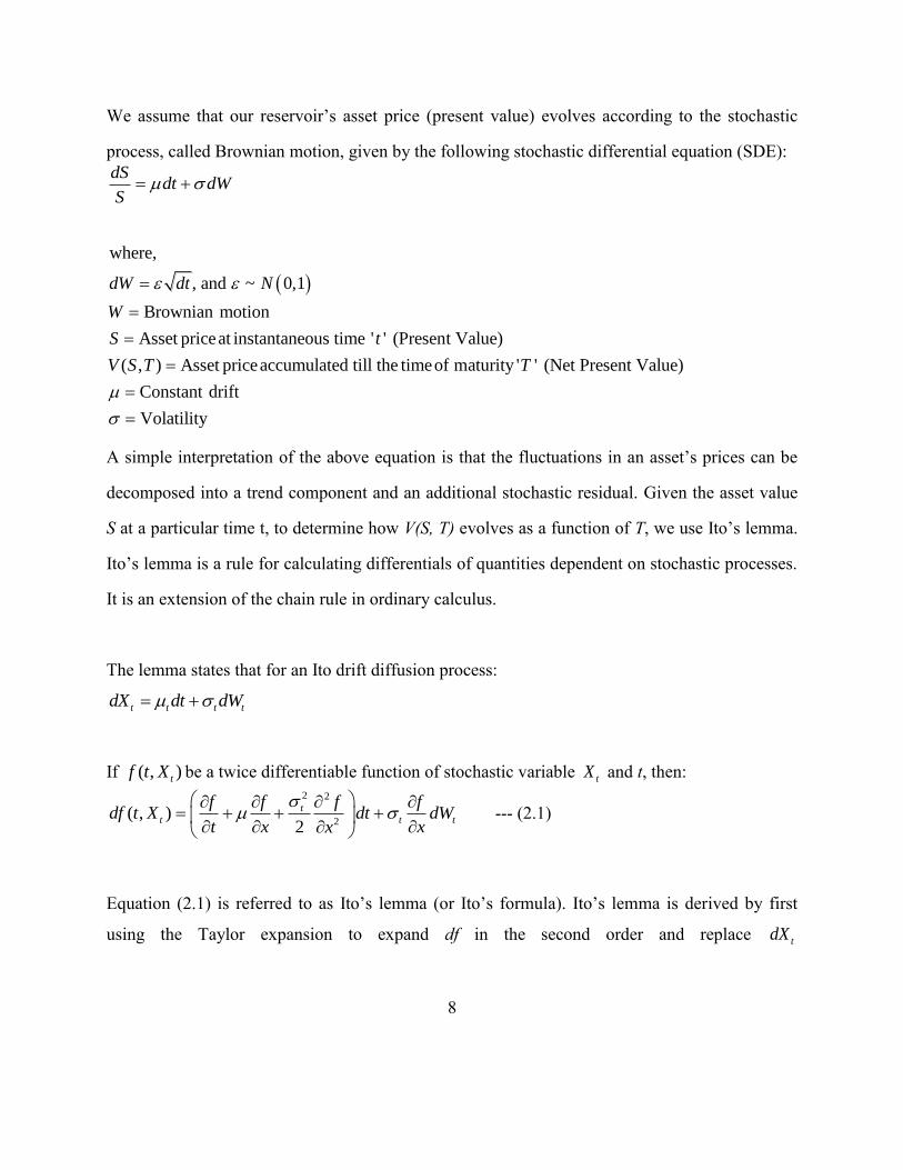
8
We assume that our reservoir‟s asset price (present value) evolves according to the stochastic
process, called Brownian motion, given by the following stochastic differential equation (SDE):
dSdt dW
S
where,
, and ~ 0,1
Brownian motion
Asset priceat instantaneous time ' ' (Present Value)
( , ) Asset priceaccumulated till the timeof maturity ' ' (Net Present Value)
Constant drift
Volatility
dW dt N
W
S t
V S T T
A simple interpretation of the above equation is that the fluctuations in an asset‟s prices can be
decomposed into a trend component and an additional stochastic residual. Given the asset value
S at a particular time t, to determine how V(S, T) evolves as a function of T, we use Ito‟s lemma.
Ito‟s lemma is a rule for calculating differentials of quantities dependent on stochastic processes.
It is an extension of the chain rule in ordinary calculus.
The lemma states that for an Ito drift diffusion process:
t t t tdX dt dW
If ( , )tf t X be a twice differentiable function of stochastic variable tX and t, then:
2 2
2( , )
2
t
t t t
f f f fdf t X dt dW
t x xx
--- (2.1)
Equation (2.1) is referred to as Ito‟s lemma (or Ito‟s formula). Ito‟s lemma is derived by first
using the Taylor expansion to expand df in the second order and replace tdX
9
with t t t tdX dt dW . The second degree terms are ignored and 2( )dW term is substituted
with dt.
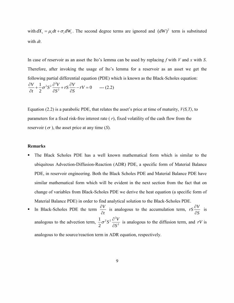
In case of reservoir as an asset the Ito‟s lemma can be used by replacing f with V and x with S.
Therefore, after invoking the usage of Ito‟s lemma for a reservoir as an asset we get the
following partial differential equation (PDE) which is known as the Black-Scholes equation: 2
2 2
2
10
2
V V VS rS rV
t S S
--- (2.2)
Equation (2.2) is a parabolic PDE, that relates the asset‟s price at time of maturity, V(S,T), to
parameters for a fixed risk-free interest rate ( r), fixed volatility of the cash flow from the
reservoir ( ), the asset price at any time (S).
Remarks
The Black Scholes PDE has a well known mathematical form which is similar to the
ubiquitous Advection-Diffusion-Reaction (ADR) PDE, a specific form of Material Balance
PDE, in reservoir engineering. Both the Black Scholes PDE and Material Balance PDE have
similar mathematical form which will be evident in the next section from the fact that on
change of variables from Black-Scholes PDE we derive the heat equation (a specific form of
Material Balance PDE) in order to find analytical solution to the Black-Scholes PDE.
In Black-Scholes PDE the term V
t
is analogous to the accumulation term,
VrS
S
is
analogous to the advection term, 2
2 2
2
1
2
VS
S
is analogous to the diffusion term, and rV is
analogous to the source/reaction term in ADR equation, respectively.
10
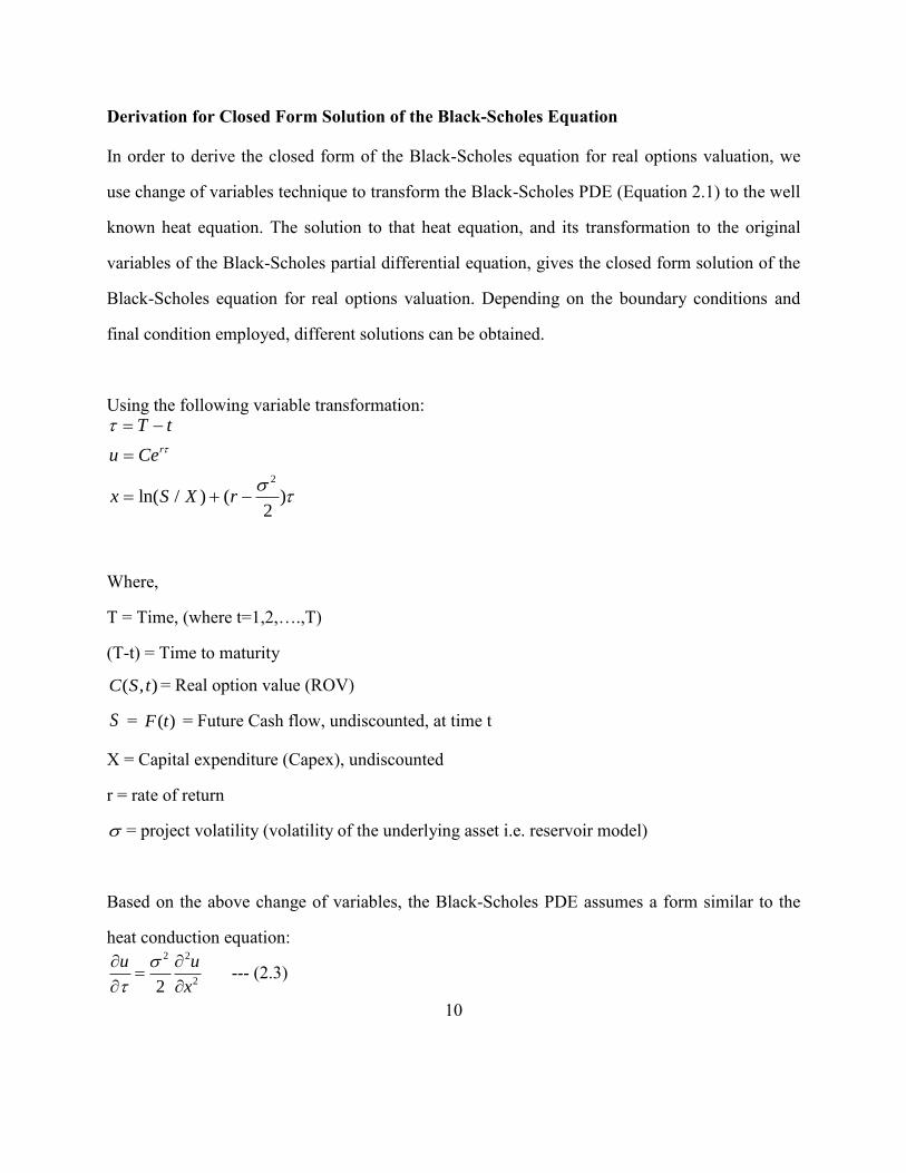
Derivation for Closed Form Solution of the Black-Scholes Equation
In order to derive the closed form of the Black-Scholes equation for real options valuation, we
use change of variables technique to transform the Black-Scholes PDE (Equation 2.1) to the well
known heat equation. The solution to that heat equation, and its transformation to the original
variables of the Black-Scholes partial differential equation, gives the closed form solution of the
Black-Scholes equation for real options valuation. Depending on the boundary conditions and
final condition employed, different solutions can be obtained.
Using the following variable transformation:
2
ln( / ) ( )2
r
T t
u Ce
x S X r
Where,
T = Time, (where t=1,2,….,T)
(T-t) = Time to maturity
( , )C S t = Real option value (ROV)
S = ( )F t = Future Cash flow, undiscounted, at time t
X = Capital expenditure (Capex), undiscounted
r = rate of return
= project volatility (volatility of the underlying asset i.e. reservoir model)
Based on the above change of variables, the Black-Scholes PDE assumes a form similar to the
heat conduction equation: 2 2
22
u u
x
--- (2.3)

11
In order to solve this PDE (Equation 2.3), we need to specify the final condition and boundary
conditions. Because at the time of maturity T, the value of a call option is exactly known, we get
the following final condition and boundary conditions, respectively:
F.C: ( , ) max( ,0)C S T S X
1 B.C: ( , ) as
2 B.C: (0, ) 0 for all
st
nd
C S t S S
C t t
The first boundary condition states that if the future cash flow goes to infinity, the value of the
option will equal the value of the future cash flow. The second boundary condition states that the
option to delay is worthless if the future cash flows are zero.
Using the above final condition and boundary conditions, we get one of the closed form solution
of the Black-Scholes equation which is also known as the real options equation (Ugur 2008):
( )
1 2( , ) ( ) ( )r T tC S t SN d Xe N d --- (2.4)
1 2 1 2
2
1 2 1
Where,
( )and ( ) cumulative normal probability values of d and d
ln ( )( )2
, and
N d N d
Sr T t
Xd d d T t
T t
S = ( )F t = Future Cash flow, undiscounted, at time t
X = Capital expenditure (Capex), undiscounted
r = rate of return
= the project volatility (volatility of the underlying asset i.e. reservoir model)
T = Time, (where t=1, 2,…., T)
12
(T-t) = Time to maturity
( , )C S t = Real option value (ROV)
Conceptually, the term 1( )N d is the probability that the value of the option will pay off, and
2( )N d is the probability that the option will be exercised (DePamphilis 2009). Mathematically,
these two terms are the Z scores from the normal probability function. These terms take risk into
account.
Remarks on ROV
In traditional ROV implementations, the price of oil is a major factor driving S and . In
subsequent chapters we incorporate geologic uncertainty into the computation of S and .
Option value = max (value, 0). Option value is not negative because philosophically it is
defined as our right but not the obligation to make the investment, never wanting to run into
loss.
Traditional Project Volatility Model
The volatility of a particular property is a statistical measure of the dispersion of that property
under given condition. Volatility of the ROV model, or project volatility, refers to the frequency
and severity with which the economic returns for a particular project fluctuate.
Volatility significantly impacts option valuation, and it is perhaps the most difficult and critical
factor to quantify. Higher volatility increases the possible option values and lower volatility
decreases the possible option values. Volatility is the only variable quantity which affects option
values and which is not directly evident either in the option type or in the market. It must be
estimated and estimating the underlying asset (reservoir) volatility is one of the most important
problems faced by practitioners wanting to use real options models. It is difficult to estimate

13
volatility in practice, because before project execution, it is impossible to assess the fluctuations
of the underlying real asset and the very process of exercising an option will introduce
fluctuations that are impossible to assess a priori. It may be useful to estimate the volatility for
the project without options by considering the project without options as the underlying asset.
There are several approaches, some of which are briefly reviewed next:
Logarithmic Ratio Method:
In this approach, the ratio of the present value at two successive time instants are calculated and
used to define the volatility as the sample standard deviation:
2
1
1
1
n
i
i
x xn
--- (2.5)
where, 1
ln i
i
PVx
PV
and x is the mean ratio over all time instants. The project volatility is thus
the sample standard deviation of the ratio of present value at successive time instants.
This method is simple and easy to use; however it does not work well if the cash flows are
negative over certain period of time as the logarithm of a negative number does not exist.
An alternative is to consolidate all future cash flow values into two sets of present values in the
following way (Mun 2002):
1
0
ln
n
i
i
n
i
i
PV
G
PV
--- (2.6)
The volatility is calculated as the standard deviation of G.

14
However both approaches (EquationS 2.5 and 2.6) are unreliable if some of the cash flows are
negative.
Copeland and Antikarov Method:
Copeland and Antikarov (Copeland & Antikarov 2001) presented a method to estimate the
volatility parameter in ROV based on hypothetical simulated distribution of returns to account
for the lack of historical distribution of returns from a project. For each simulation trial, the value
of the returns is estimated at two different points in time. These two estimates are generated
independently because it is assumed that the value of a project through time will follow a random
walk, regardless of the pattern of cash flows (Samuelson 1965). The ratio of these two estimated
underlying asset values gives an estimate of the rate of return. A rate of return distribution is
generated by compiling the rate of return estimates from all simulations.
The detailed steps for calculating the project volatility by the Copeland and Antikarov method
are outlined below:
(0)F = Known cash flow in year 0
( )F t = [Future incoming cash flow (revenue) – Opex] = Uncertain cash flow in the tth
year,
where t=1, 2,…., T
r = continuously compounded discount rate (the rate used to discount future cash flows to their
present values)
( )MV n = Market value of the project at time n (expectation over the future cash flows)
( )PW n = Present worth of the project at time n (expectation over the future cash flows)
( )k n = a random variable that represents the continuously compounded rate of return on the
project between time n-1 and time n.
15
The present value at any time t is calculated by multiplying the future cash flow, ( )F t , with the
discount factor, ( )DV t i.e.
( ) ( ) ( )PV t F t DV t
For a fixed discount rate, r, discretely compounded over time, t:
1( )
(1 )tDV t
r
For a fixed continuously compounded discount rate:
( ) rtDV t e
Denoting the present value at time n of future cash flows as MV(n):
( )
1
( ) ( ).T
r t n
t n
MV n F t e
Adding the cash flow at time n, we get the present worth PW(n).
( )( ) ( ) ( ) ( ).T
r t n
t n
PW n MV n F n F t e
In other words:
( )( ) ( 1). k nPW n MV n e
( )
andso ( ) ln( 1)
PW nk n
MV n
--- (2.7)
Since the cash flows are uncertain, the corresponding PW(n) are actually random variables
(outcomes from simulation). We therefore get a distribution for ( )k n using equation (2.7) and the
standard deviation of this distribution is the project volatility i.e.
( ) ( )n std k n

16
If the volatility of the project changes with time, this method can still be used to compute time
varying volatility by computing distributions of k for different times and standard deviation of
each k will generate volatility for each year.
The Oil Price Model
The three types of processes used in modeling financial commodities are geometric Brownian
motion (GMB) process, Mean Reverting (MR) process, and mean reversion with jumps (MRJ)
process. However, mean reverting (MR) processes are the most widely used to model financial
commodities. Ornstein and Uhlenbeck (Ornstein & Uhlenbeck 1930) is the most popular MR
model.
Mean reverting processes incorporate the concept of demand and supply i.e. when prices are „too
high‟, demand will reduce and supply will increase, producing a counter-balancing effect. When
prices are „too low‟ the opposite will occur, again pushing prices back towards the long term
mean. Some of the properties of this model are:
The price is said to follow MR process if price follows a log-normal diffusion.
Price changes in MR models are not independent.
MR models have a long term equilibrium price and mean reversion rate.
The Ornstein-Uhlenbeck method is widely used for modelling a mean reverting process. We start
by defining the terms and some concepts to be used:
tW = a Brownian- Motion, also called Weiner process. ~ (0, )tdW N dt
17
= the speed of mean reversion
= the „long run mean‟, to which the process tends to revert.
= a measure of the process volatility
t = time
t = small time
tP = Price of oil at time„t‟
Now we present the formulae to be used based on Ornstein-Uhlenbeck model (Dias 2004).
The process of fluctuation in oil price „P‟ is modeled as:
( ) tdP P dt dW
--- (2.8)
The exact formula of the Ornstein-Uhlenbeck mean reverting process which is obtained as a
solution to the differential equation (2.8) that holds for any size of t is: 2
1
(1 )(1 )
2
tt t
t t t
eP e P e dW
To estimate the three parameters of MR model, we must have historical data of oil price. Then
parameter estimation can be done using well known techniques for parameter estimation such as
Least Square regressions, and Maximum Likelihood.
Once we have historical data of oil prices, we can examine the distribution of annual changes in
the natural logarithm of price, as oil prices are usually said to follow a log-normal distribution.
Instead of using deterministic values for long-term mean, reversion speed and volatility of oil
prices, we can replace them with their distribution values (min., most likely and max.).
18
Chapter 3: Model Updating and Value of Information
INTRODUCTION
This chapter presents:
An economic analysis procedure that accounts for uncertainty in production forecasts
arising due to incomplete geologic information.
A procedure to assess the worth of progressive updating of reservoir models using
additional data.
For the first objective, a workflow to model reservoir uncertainty and its economic analysis is
presented and a procedure for economic analysis is developed. The workflow also demonstrates
how to incorporate flow rate uncertainty in the ROV calculations.
For the second objective of our research, we compared the value of information obtained by
either drilling an additional exploratory well or acquiring seismic for developing a reservoir
model. The base case reservoir model is obtained conditioned data along 5 production wells and
the value of information is assessed both in terms of uncertainty reduction and increase in
economic returns. Even though in this particular case neither of the two information brought
significant improvement to the economic forecast over the base case forecast, the example
demonstrates the workflow for updating reservoir models and assessing the value of information.
19
RESEARCH APPROACH
For geostatistical modeling we used stochastic simulation algorithms like sequential Gaussian
Simulation SGSIM (Deutsch & Journel 1997), and cosimulation COSGSIM (Xu et al. 1992). We
used the histogram transformation program TRANS to ensure that the final stochastic reservoir
models reflect the target histogram accurately. For these techniques we performed variogram.
Through geostastical modeling we get multiple realizations of porosity and permeability models.
For flow modeling we used the CMG simulator (CMG-IMEX 2009) in order to obtain
production rates. Geostatistical modeling followed by flow modeling is essential for uncertainty
assessment of reservoir performance. Finally for economic analysis we use a deterministic
discounted cash flow (DCF) technique, as well as real options valuation (ROV) that utilize the
uncertainty models explicitly.
INCORPORATING RESERVOIR UNCERTAINTY IN ROV
An algorithm is presented to forecast reservoir flow uncertainty and its corresponding economic
analysis. The steps for incorporating flow rate uncertainty in the ROV calculations are:
I. We develop multiple realizations of reservoir model using appropriate geostatistical
technique.
II. These stochastic reservoir models are then input into the reservoir flow simulator to
determine future hydrocarbon production rates. We obtain as many realizations of
production rates as the number of stochastic reservoir models. The uncertainty in the
stochastic reservoir models is carried to the hydrocarbon production rates. This
uncertainty is represented by the different realizations of production rate profiles.
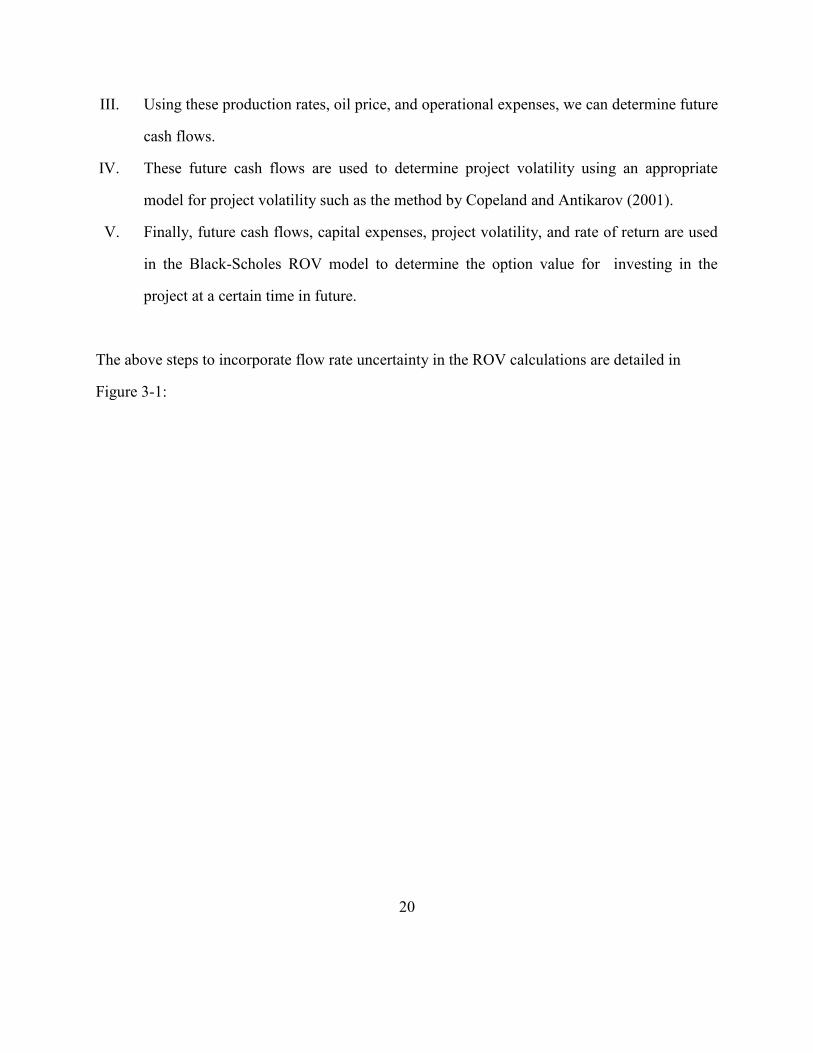
20
III. Using these production rates, oil price, and operational expenses, we can determine future
cash flows.
IV. These future cash flows are used to determine project volatility using an appropriate
model for project volatility such as the method by Copeland and Antikarov (2001).
V. Finally, future cash flows, capital expenses, project volatility, and rate of return are used
in the Black-Scholes ROV model to determine the option value for investing in the
project at a certain time in future.
The above steps to incorporate flow rate uncertainty in the ROV calculations are detailed in
Figure 3-1:

21
Algorithm
Figure 3-1: Algorithm for incorporating reservoir uncertainty in ROV
As pointed out in the previous chapter, N(d1) and N(d2) are normal probability values
corresponding to d1 and d2 that can be calculated knowing the cash flow, rate of return r and
Multiple realizations of reservoir model using
an appropriate geostatistical technique
Multiple realizations of production rates (q) by
inputting stochastic reservoir models in a reservoir flow
simulator
Using these production rates, oil price, and operational
expenses, we can determine future cash flows.
( ) ( )F t q t p opex
( )S F t
X capex
Determine project volatility
using ( )F t and an appropriate
method such as Copeland and
Antikarov.
( ) ( )
1 2( , ) ( ) ( )r t r tC S t Se N d Xe N d
22
project volatility . The algorithm above describes the workflow of converting the reservoir
uncertainty into economic returns from the reservoir.
ASSESSING THE VALUE OF INFORMATION
Description of the Problem
We assume a reservoir with grid dimension of 50 x 50 x 1 that initially has 5 production wells
only. Basic information available about the reservoir characteristics such as porosity and
permeability is from these 5 production wells. Using this base information we can develop
multiple realizations of the reservoir model and future economic performance of the reservoir.
Having multiple scenarios for economic performance of the reservoir enables us to perform risk
analysis and take appropriate decisions regarding further development of the reservoir.
These multiple realizations of future economic performance of the reservoir represent
uncertainty, and in order to reduce this uncertainty in predicting future economic performance
we need to gain more information about our reservoir. We can adopt one of the following two
ways to gain reservoir information:
Scenario 1: Drill an exploratory well – This will yield core data that can be directly used as
“hard” conditioning data for the next generation of models
Scenario 2: Acquire seismic (secondary data which mimics seismic was generated by taking
moving window average of a porosity model that was developed for the base case) – This would
be reflective of “soft” data that is at a resolution different from the “hard” conditioning data and
is imprecisely related to the “hard” data.
23
Gaining extra information, over and above the existing 5 producing wells, may reduce the
uncertainty of our forecasted economic returns and give a more correct estimate for the economic
value of the field. Our objective is to evaluate which of two different types of information gives
more accurate future economic forecast and more reliable models of uncertainty.
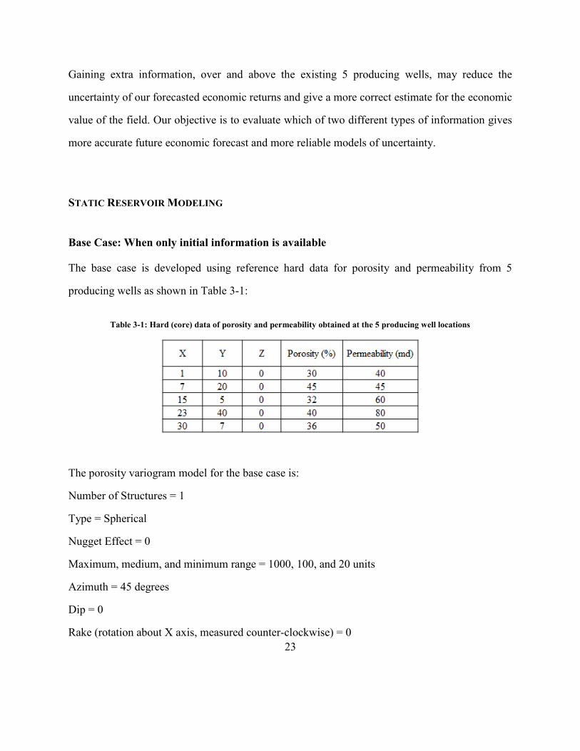
STATIC RESERVOIR MODELING
Base Case: When only initial information is available
The base case is developed using reference hard data for porosity and permeability from 5
producing wells as shown in Table 3-1:
Table 3-1: Hard (core) data of porosity and permeability obtained at the 5 producing well locations
The porosity variogram model for the base case is:
Number of Structures = 1
Type = Spherical
Nugget Effect = 0
Maximum, medium, and minimum range = 1000, 100, and 20 units
Azimuth = 45 degrees
Dip = 0
Rake (rotation about X axis, measured counter-clockwise) = 0
24
The permeability variogram model for the base case is:
Number of Structures = 1
Type = Spherical
Nugget Effect = 0
Max., medium, and min. range = 1500, 200, and 0 units
Azimuth = 30 degrees
Dip = 0
Rake = 0
To obtain multiple realizations of porosity maps, hard data of porosity and variogram model for
porosity are used as input in the Sequential Gaussian Simulation SGSIM geostastical program
(Remy et al. 2009). In this algorithm, the local conditional probability distribution at each
unknown location on the grid is obtained by kriging using the hard data and previously simulated
values in the vicinity of that node. A simulated value is sampled at random from the local
conditional probability distribution and that value is added to the conditioning data set at the next
simulation node visited along a random path. In this way, the simulation reproduces hard data
histogram, and honors spatial variability as indicated by the variogram.
To obtain multiple realizations of permeability maps, hard data of permeability and a model of
porosity are specified as primary and secondary data, respectively, along with variogram model
for permeability. The Gaussian co-simulation program - COSGSIM (Remy et al. 2009) is used
for the simulation. The correlation between primary and secondary variables was assumed as 0.6.
In this simulation, the local conditional probability distribution at the simulation node is obtained
by cokriging i.e. by extending the estimator to include the conditioning influence of the
25
secondary porosity data. The interaction between the primary and the secondary variable is
approximated using a Markov hypothesis (Remy et al., 2009 [4]) and the specified correlation
coefficient. Other than this extended procedure for constructing the local distribution, the
remaining steps for sequential simulation are the same..
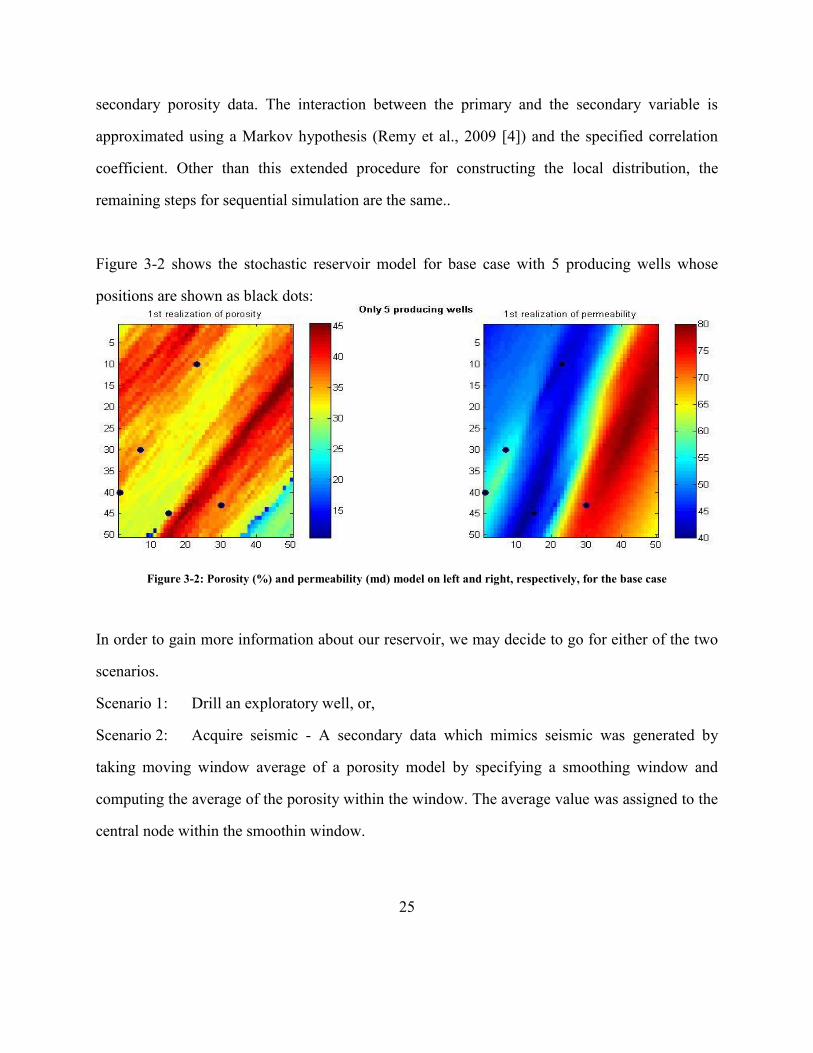
Figure 3-2 shows the stochastic reservoir model for base case with 5 producing wells whose
positions are shown as black dots:
Figure 3-2: Porosity (%) and permeability (md) model on left and right, respectively, for the base case
In order to gain more information about our reservoir, we may decide to go for either of the two
scenarios.
Scenario 1: Drill an exploratory well, or,
Scenario 2: Acquire seismic - A secondary data which mimics seismic was generated by
taking moving window average of a porosity model by specifying a smoothing window and
computing the average of the porosity within the window. The average value was assigned to the
central node within the smoothin window.
26
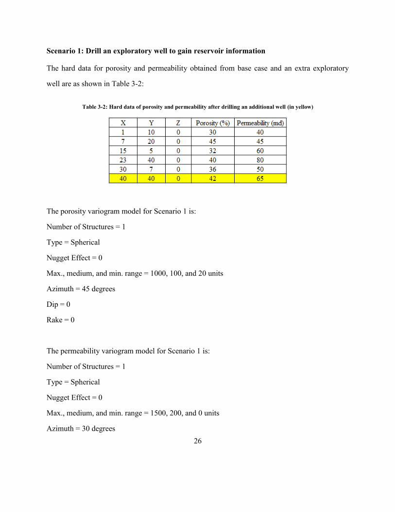
Scenario 1: Drill an exploratory well to gain reservoir information
The hard data for porosity and permeability obtained from base case and an extra exploratory
well are as shown in Table 3-2:
Table 3-2: Hard data of porosity and permeability after drilling an additional well (in yellow)
The porosity variogram model for Scenario 1 is:
Number of Structures = 1
Type = Spherical
Nugget Effect = 0
Max., medium, and min. range = 1000, 100, and 20 units
Azimuth = 45 degrees
Dip = 0
Rake = 0
The permeability variogram model for Scenario 1 is:
Number of Structures = 1
Type = Spherical
Nugget Effect = 0
Max., medium, and min. range = 1500, 200, and 0 units
Azimuth = 30 degrees
27
Dip = 0
Rake = 0
To obtain multiple realizations of porosity maps after conditioning to the extra information at the
exploratory well location, the SGSIM geostatistical program was used. Once the porosity
realizations were generated, permeability realization was obtained by conditioning to the hard
permeability data as well as the previously simulated porosity model. In order to keep the
simulation combinatorial manageable, the simulation was performed by only conditioning to one
of the realizations of porosity. The correlation coefficient between porosity and permeability was
again assumed to be 0.6.
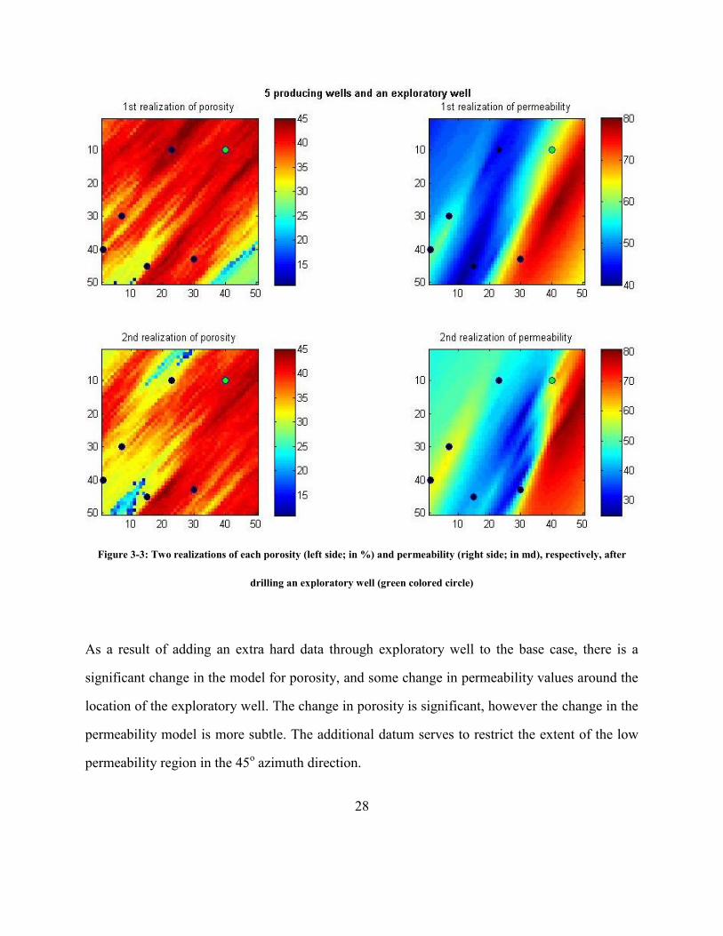
Figure 3-3 shows the updated reservoir model obtained after conditioning to one extra
exploratory well data. Black dots represent position of 5 producing wells from the base case,
while green dots represent position of exploratory well.
28
Figure 3-3: Two realizations of each porosity (left side; in %) and permeability (right side; in md), respectively, after
drilling an exploratory well (green colored circle)
As a result of adding an extra hard data through exploratory well to the base case, there is a
significant change in the model for porosity, and some change in permeability values around the
location of the exploratory well. The change in porosity is significant, however the change in the
permeability model is more subtle. The additional datum serves to restrict the extent of the low
permeability region in the 45o azimuth direction.
29
Scenario 2: Acquiring Seismic to gain reservoir information
We generate secondary data which mimics seismic by taking moving window average of a
porosity model that was developed for the base case. The primary data for porosity and
permeability are the 5 hard data from the base case. The variogram models for both porosity and
permeability are same for this Scenario.
The porosity and permeability variogram model for Scenario 2 is:
Number of Structures = 1
Type = Spherical
Nugget Effect = 0
Max., medium, and min. range = 1500, 200, and 0 units
Azimuth = 30 degrees
Dip = 0
Rake = 0
To obtain multiple realizations of porosity maps conditioned to primary hard data of porosity and
secondary (mimicking seismic) data the COSGSIM geostatistical program was used. The
correlation between primary and secondary variables was assumed as 0.6.
Similarly, to obtain multiple realizations of permeability maps, hard data of permeability and any
one model of updated porosity (from Scenario 2) were used as primary and secondary data,
respectively, along with variogram model for permeability. Cosimulation (COSGSIM) was
performed. The correlation between primary and secondary variables was assumed as 0.6.
30
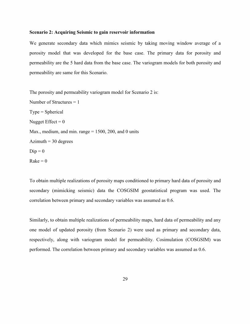
Figure 3-4a shows the secondary data which mimics the seismic and Figure 3-4b shows the
updated reservoir model obtained after conditioning to the secondary data that mimics seismic.
Black dots represent position of 5 producing wells from the base case.
(a)
(b)
Figure 3-4: a) Secondary data mimicking seismic; b) Two realizations of each porosity (%) and permeability (md) model
on left and right, respectively, after acquiring seismic
31
As a result of adding extra information in the form of seismic data to the base case, there is a
significant change in new geological models for both porosity and permeability. Porosity models
updated after acquiring seismic are much smoother compared to the porosity model for the base
case or porosity models updated after acquiring data from exploratory well. There is also
significant change in permeability models updated after acquiring seismic compared to the
permeability model for the base case or permeability models updated after acquiring data from
exploratory well.
FLOW MODELING
After obtaining static reservoir models for porosity and permeability from geological models, as
shown in Figures 3-2 to 3-4, we can input them in a flow model to generate future oil production
forecast for the entire life of the reservoir. The following fluid, reservoir and well parameters
were assumed for the flow modeling.
Fluid Properties
6 -1
0.65cp
2 10 psi
1.54B/STB
t
o
c
B
Reservoir and Well Properties
Area = 0.36million acres
No. of production wells = 5
(Shape factor for square reservoir) 31.62
Skin = 5
3500psi
A
i
C
P
32
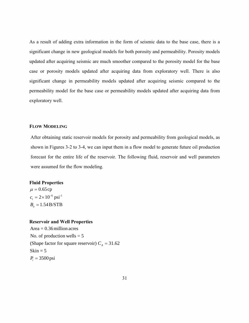
Figure 3-5 shows the oil-water two phase relative permeability curve.
Figure 3-5: Two phase relative permeability curve for oil-water phase
We input these properties and multiple realizations of the static reservoir models in the CMG to
get multiple responses from the flow model. Figure 3-6 shows one of the reservoir models setup
in CMG gridded for flow with grid dimension of 50 x 50 x 1. There are five production wells
which are producing hydrocarbons through natural water drive without the need of any injectors.
The wells are located at the locations given in Table 3-1:
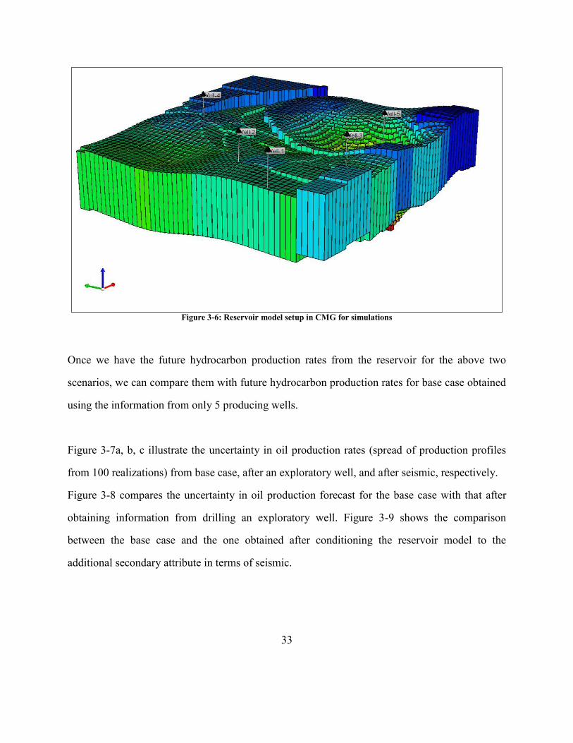
33
Figure 3-6: Reservoir model setup in CMG for simulations
Once we have the future hydrocarbon production rates from the reservoir for the above two
scenarios, we can compare them with future hydrocarbon production rates for base case obtained
using the information from only 5 producing wells.
Figure 3-7a, b, c illustrate the uncertainty in oil production rates (spread of production profiles
from 100 realizations) from base case, after an exploratory well, and after seismic, respectively.
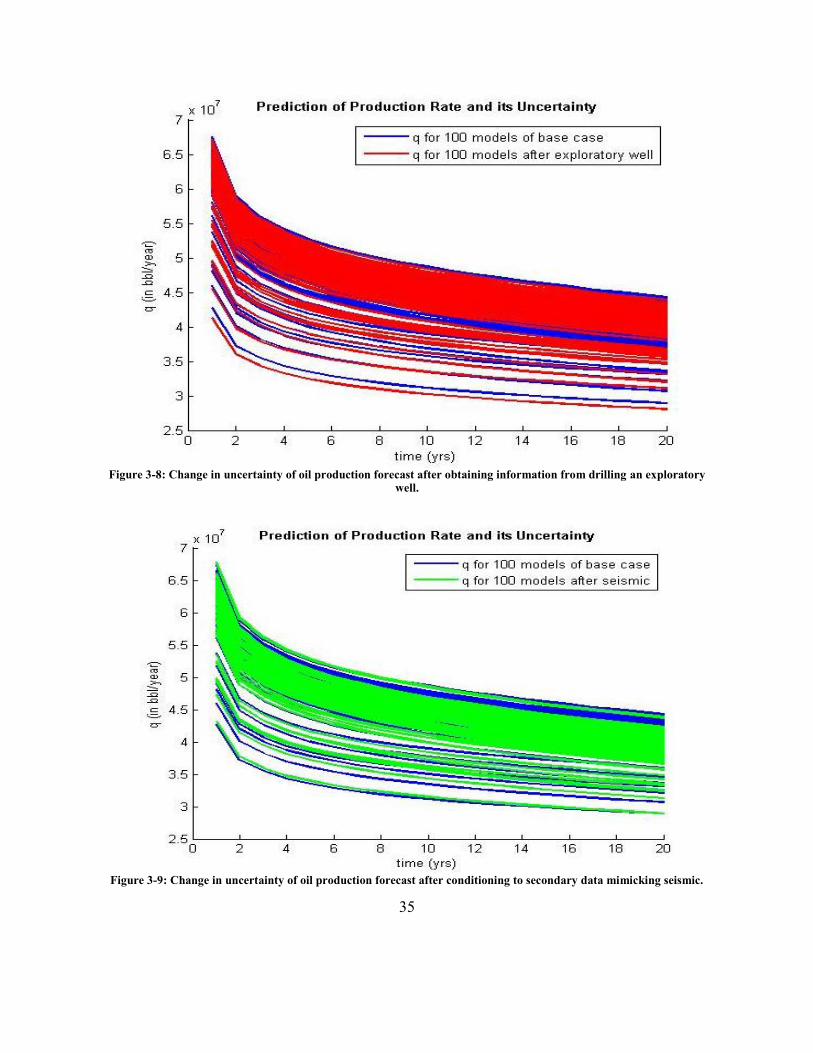
Figure 3-8 compares the uncertainty in oil production forecast for the base case with that after
obtaining information from drilling an exploratory well. Figure 3-9 shows the comparison
between the base case and the one obtained after conditioning the reservoir model to the
additional secondary attribute in terms of seismic.
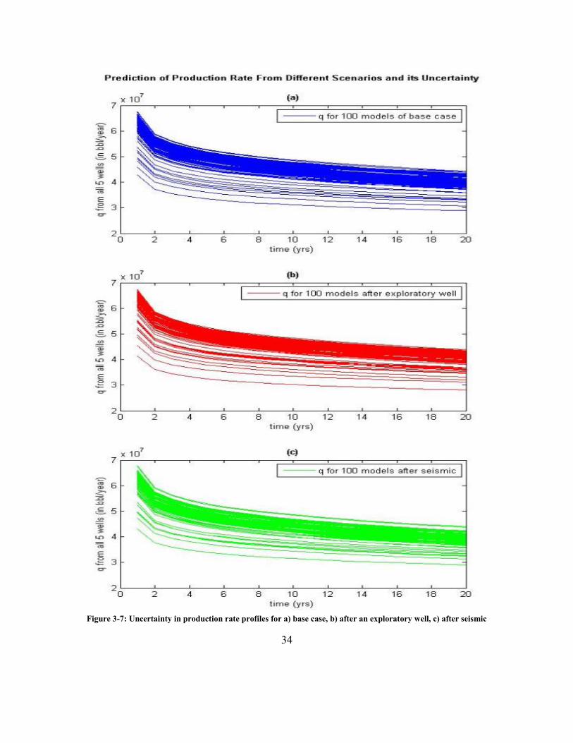
34
Figure 3-7: Uncertainty in production rate profiles for a) base case, b) after an exploratory well, c) after seismic
35
Figure 3-8: Change in uncertainty of oil production forecast after obtaining information from drilling an exploratory
well.
Figure 3-9: Change in uncertainty of oil production forecast after conditioning to secondary data mimicking seismic.
36
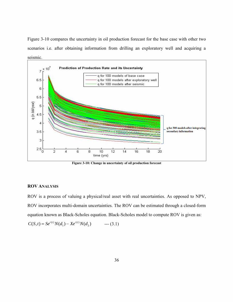
Figure 3-10 compares the uncertainty in oil production forecast for the base case with other two
scenarios i.e. after obtaining information from drilling an exploratory well and acquiring a
seismic.
Figure 3-10: Change in uncertainty of oil production forecast
ROV ANALYSIS
ROV is a process of valuing a physical/real asset with real uncertainties. As opposed to NPV,
ROV incorporates multi-domain uncertainties. The ROV can be estimated through a closed-form
equation known as Black-Scholes equation. Black-Scholes model to compute ROV is given as:
--- (3.1)
( ) ( )
1 2( , ) ( ) ( )r t r tC S t Se N d Xe N d
37
2
1 2 1
where,
( , ) ROV
ln ( )( )2
,
C S t
Sr T t
Xd and d d T t
T t
( )
capex
12%
Project Volatility
Time period of maturity
S F t
X
r
T
Once we determine the future oil production rates as illustrated in previous section, the following
equation is used to obtain forecast of future cash flows for each realization of q(t):
( ) ( )F t q t p opex --- (3.2)
In equation (3.2) production rate is the only variable that is allowed to vary with time. Oil price
can be made to vary by computing time varying oil prices using the Ornstein and Uhlenbeck
mean reverting model; however, oil prices are kept constant at $ 30/barrel to have consistent
comparison of the reservoir economic performance by different geological models.
These future cash flows will be used to compute the project volatility through the method
explained in Chapter 2. This project volatility is one of the most critical parameter which is used
as input in the real options model. We calculated the project volatility as following:
( ) ( ) ( )PV t F t DV t
38
1
0
h
ln
( )
where,
Present value at i year
std( ) Standard deviation
Project Volatility
n
i
i
n
i
i
t
i
PV
G
PV
std G
PV
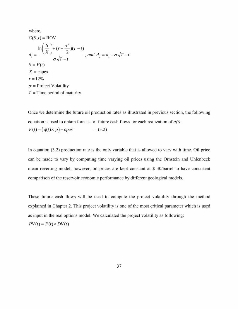
Figure 3-11 shows the time varying project volatility‟s magnitude decreasing with time. The
reason for the decrease in project volatility with time is because there is more prior data of the
reservoir‟s economic performance (in terms of DCF).
Figure 3-11: Variation of project volatility with time during the life of the reservoir

39
ROV can be obtained on substituting values for the above variables in equation (3.1). The above
calculation is repeated for all the realizations to come up with the uncertainty in the ROV.
RESULTS AND DISCUSSIONS
The cumulative sum of present values gives Net Present Value (or cumulative DCF) which is
shown in Figure 3-12. Figure 3-12 compares the uncertainty in cumulative DCF forecast for the
base case with that after obtaining information from drilling an exploratory well or aquiring
seismic.
Figure 3-12: Comparison of uncertainty in cumulative DCF for scenarios 1 and 2 with base case
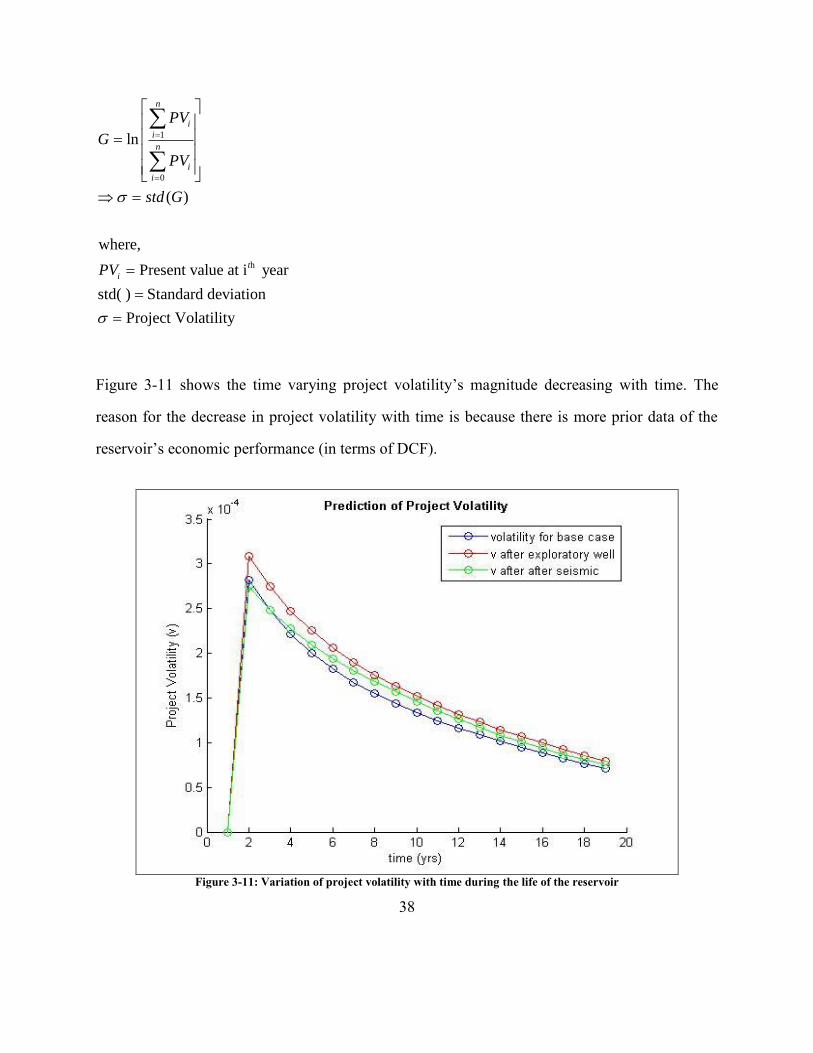
Figure 3-13 compares the uncertainty in ROV for the base case with other two scenarios i.e. after
obtaining information from drilling an exploratory well and after conditioning to the secondary
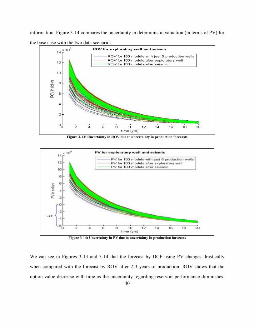
40
information. Figure 3-14 compares the uncertainty in deterministic valuation (in terms of PV) for
the base case with the two data scenarios
Figure 3-13: Uncertainty in ROV due to uncertainty in production forecasts
Figure 3-14: Uncertainty in PV due to uncertainty in production forecasts
We can see in Figures 3-13 and 3-14 that the forecast by DCF using PV changes drastically
when compared with the forecast by ROV after 2-3 years of production. ROV shows that the
option value decrease with time as the uncertainty regarding reservoir performance diminishes.
41
Comparing the profile of the ROV to that of PV, the ROV analysis preserves the uncertainty in
reservoir characteristics till the very end, while the uncertainty in present value decreases
practically to zero at the end time
The results further show that both schemes for acquiring additional reservoir related information
result in similar reduction in prior uncertainty. The added cost of drilling an additional well or
acquiring secondary data causes the DCF value to decrease below zero at later times. However,
the ROV by construction, does not dip below zero (option is not exercised if the PV is negative).
Even though the ROV is positive for all scenarios (base case, drill an exploratory well, or acquire
seismic), there is insignificant monetary gain by acquiring additional reservoir related
information over the base case. Therefore, it would not be a judicious decision to invest in either
of the scheme for acquiring additional reservoir related information.

42
Chapter 4: Assessing Economic Implications of Reservoir Modeling Decisions
INTRODUCTION
This chapter presents a method for:
Using real option valuation to assess the economic forecast of reservoir performance
using geological models of varying levels of complexity.
Using real option valuation to assess the economic forecast of reservoir performance
using flow models of varying levels of complexity.
For the first objective, we compared the uncertainty in reservoir‟s long term performance
obtained by geological models with varying levels of complexity. The results suggest that it may
be appropriate to use simpler geological models for the forecast of volumetric flow rate
uncertainty. We see that the economics in terms of real option value obtained from a simple
geological model is not significantly different from that of a complex geological model. Similar
results also hold true with DCF analysis.
For the second objective of our research, we compared the uncertainty in reservoir‟s long term
performance obtained by decline curve analysis and a full physics commercial simulator. The
results suggest that using decline curve as a flow model predicts the long term production rate
fairly accurately and for the case studied, is as good as using a full physics commercial
simulator.

43
These two studies help answer the question – how much detail in reservoir and flow models are
necessary if the end objective is to obtain realistic assessment of net economic risk (which would
be used to make correct decisions)?
ASSESSING THE IMPACT OF DETAILED GEOLOGICAL MODELING
Research Approach
For geostatistical modeling, we used well estiablished stochastic simulation algorithms like
sequential Gaussian Simulation SGSIM (Deutsch & Journel 1997), cosimulation COSGSIM (Xu
et al. 1992), indicator simulation SISIM (Zhu & Journel 1993) and multiple point simulation
SNESIM (Strabelle 2000). For these techniques semivariogram modeling was performed or in
the case of SNESIM, provided a training image. Geostastical modeling gives us multiple
realizations of porosity and permeability models.
For flow modeling we used the CMG simulator (CMG-IMEX 2009) and decline curve analysis
(Arps 1945) to obtain production rates. Geostatistical modeling followed by flow modeling is
essential for uncertainty assessment of reservoir performance. Finally for economic analysis we
use a deterministic discounted cash flow (DCF) technique, as well as real options valuation
(ROV) that use the uncertainty models explicitly.
Description of the Problem
The reference truth model for the reservoir has a grid dimension of 200 200 1. The reference
truth model is a truly known model for the reservoir which is used as reference/base case with
predicted models. This reservoir has 5 production wells. We use different geological models to
44
map porosity and permeability of the reservoir. Though all these techniques yield reservoir
property variations over a 3D grid; however, we use these models selectively based on the type
of reservoir information we want simulated or honored.
Some of the commonly used geological models include SGSIM, SISIM and SNESIM, in the
order of increasing complexity. Complexity is in terms of the amount and type of reservoir
information needed to generate the porosity and permeability maps as illustrated in next
paragraph; the more information a model requires, the more complex it is. Nevertheless, we must
give a certain minimum amount of information to all these 3 models, which includes
conditioning data to be honored. Other than this information each model requires more
information based on the level of complexity. SGSIM and SISIM are semivariogram-based
simulations techniques, while SNESIM is a multiple-point simulation technique. Semivariogram-
based techniques are less complex than multiple-point technique. Semivariogram is a measuare
of variability between pairs of locations in the reservoir. It can be typically inferred on the basis
of the available “hard” data. Multiple point based techniques such as SNESIM on the other hand
require inference of joint variability between several locations (more than two) in the reservoir.
Typically, inference of multiple point statistics require exhaustive training data, a spatial
template and a sohisticated scheme for scaning and saving statistics and subsequently retrieving
the same when performing conditional simulation (Eskandari, 2009). This contributes to the
complexity of the algorithm. The amount and type of data that each of these models require, in
an increasing order of complexities, are:
SGSIM: Conditioning Data + Semivariogram Model
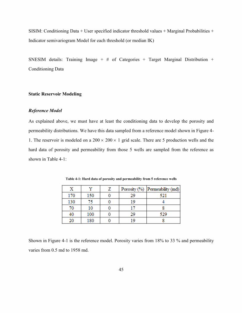
45
SISIM: Conditioning Data + User specified indicator threshold values + Marginal Probabilities +
Indicator semivariogram Model for each threshold (or median IK)
SNESIM details: Training Image + # of Categories + Target Marginal Distribution +
Conditioning Data
Static Reservoir Modeling
Reference Model
As explained above, we must have at least the conditioning data to develop the porosity and
permeability distributions. We have this data sampled from a reference model shown in Figure 4-
1. The reservoir is modeled on a 200 200 1 grid scale. There are 5 production wells and the
hard data of porosity and permeability from those 5 wells are sampled from the reference as
shown in Table 4-1:
Table 4-1: Hard data of porosity and permeability from 5 reference wells
Shown in Figure 4-1 is the reference model. Porosity varies from 18% to 33 % and permeability
varies from 0.5 md to 1958 md.
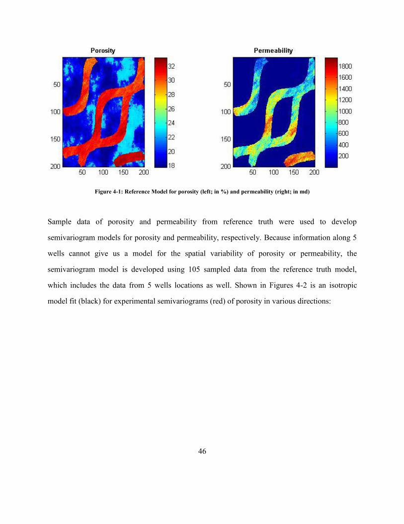
46
Figure 4-1: Reference Model for porosity (left; in %) and permeability (right; in md)
Sample data of porosity and permeability from reference truth were used to develop
semivariogram models for porosity and permeability, respectively. Because information along 5
wells cannot give us a model for the spatial variability of porosity or permeability, the
semivariogram model is developed using 105 sampled data from the reference truth model,
which includes the data from 5 wells locations as well. Shown in Figures 4-2 is an isotropic
model fit (black) for experimental semivariograms (red) of porosity in various directions:
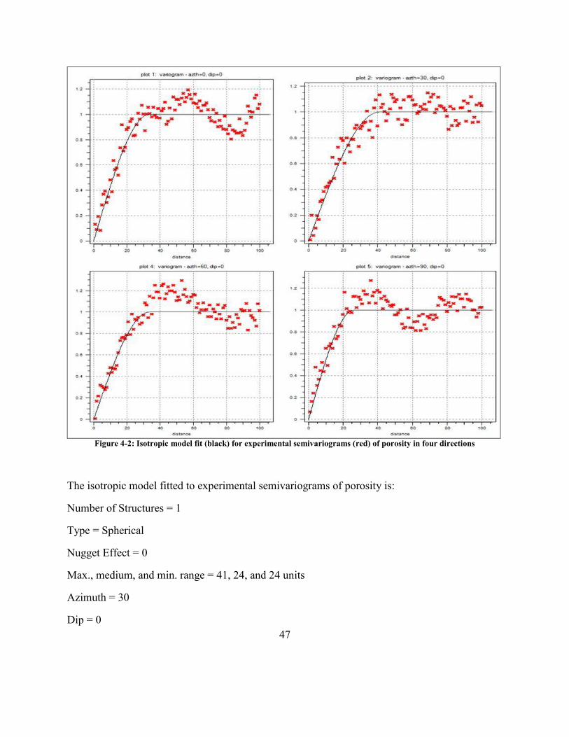
47
Figure 4-2: Isotropic model fit (black) for experimental semivariograms (red) of porosity in four directions
The isotropic model fitted to experimental semivariograms of porosity is:
Number of Structures = 1
Type = Spherical
Nugget Effect = 0
Max., medium, and min. range = 41, 24, and 24 units
Azimuth = 30
Dip = 0
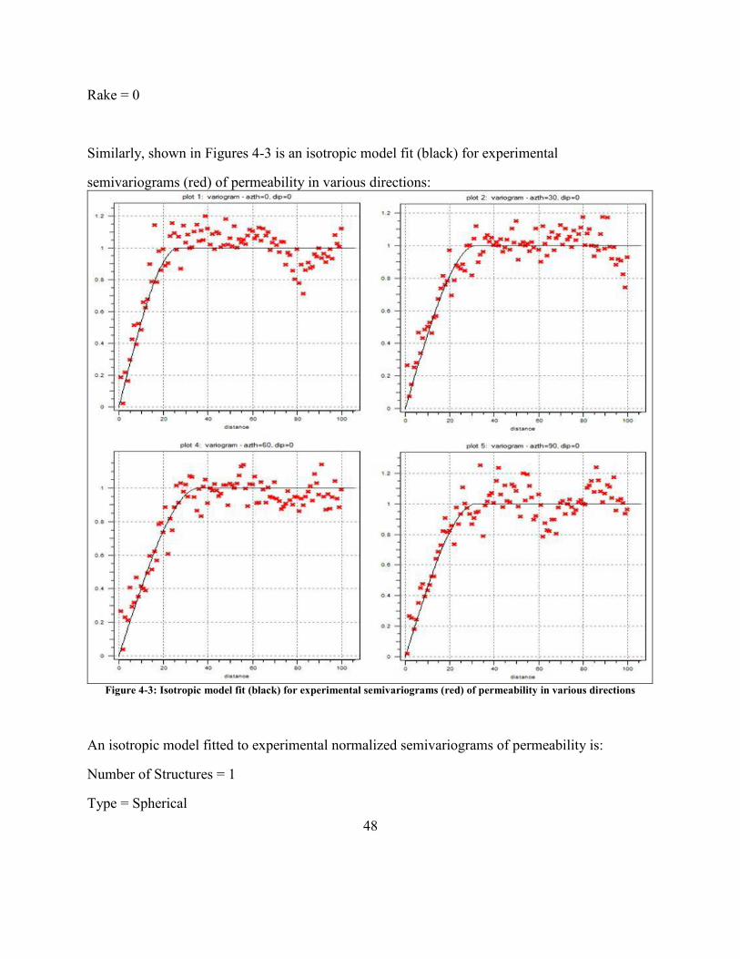
48
Rake = 0
Similarly, shown in Figures 4-3 is an isotropic model fit (black) for experimental
semivariograms (red) of permeability in various directions:
Figure 4-3: Isotropic model fit (black) for experimental semivariograms (red) of permeability in various directions
An isotropic model fitted to experimental normalized semivariograms of permeability is:
Number of Structures = 1
Type = Spherical
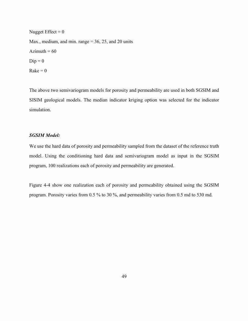
49
Nugget Effect = 0
Max., medium, and min. range = 36, 25, and 20 units
Azimuth = 60
Dip = 0
Rake = 0
The above two semivariogram models for porosity and permeability are used in both SGSIM and
SISIM geological models. The median indicator kriging option was selected for the indicator
simulation.
SGSIM Model:
We use the hard data of porosity and permeability sampled from the dataset of the reference truth
model. Using the conditioning hard data and semivariogram model as input in the SGSIM
program, 100 realizations each of porosity and permeability are generated.
Figure 4-4 show one realization each of porosity and permeability obtained using the SGSIM
program. Porosity varies from 0.5 % to 30 %, and permeability varies from 0.5 md to 530 md.
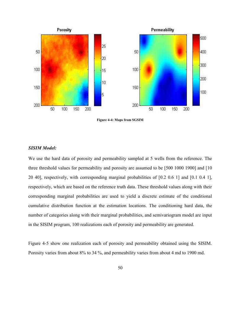
50
Figure 4-4: Maps from SGSIM
SISIM Model:
We use the hard data of porosity and permeability sampled at 5 wells from the reference. The
three threshold values for permeability and porosity are assumed to be [500 1000 1900] and [10
20 40], respectively, with corresponding marginal probabilities of [0.2 0.6 1] and [0.1 0.4 1],
respectively, which are based on the reference truth data. These threshold values along with their
corresponding marginal probabilities are used to yield a discrete estimate of the conditional
cumulative distribution function at the estimation locations. The conditioning hard data, the
number of categories along with their marginal probabilities, and semivariogram model are input
in the SISIM program, 100 realizations each of porosity and permeability are generated.
Figure 4-5 show one realization each of porosity and permeability obtained using the SISIM.
Porosity varies from about 8% to 34 %, and permeability varies from about 4 md to 1900 md.
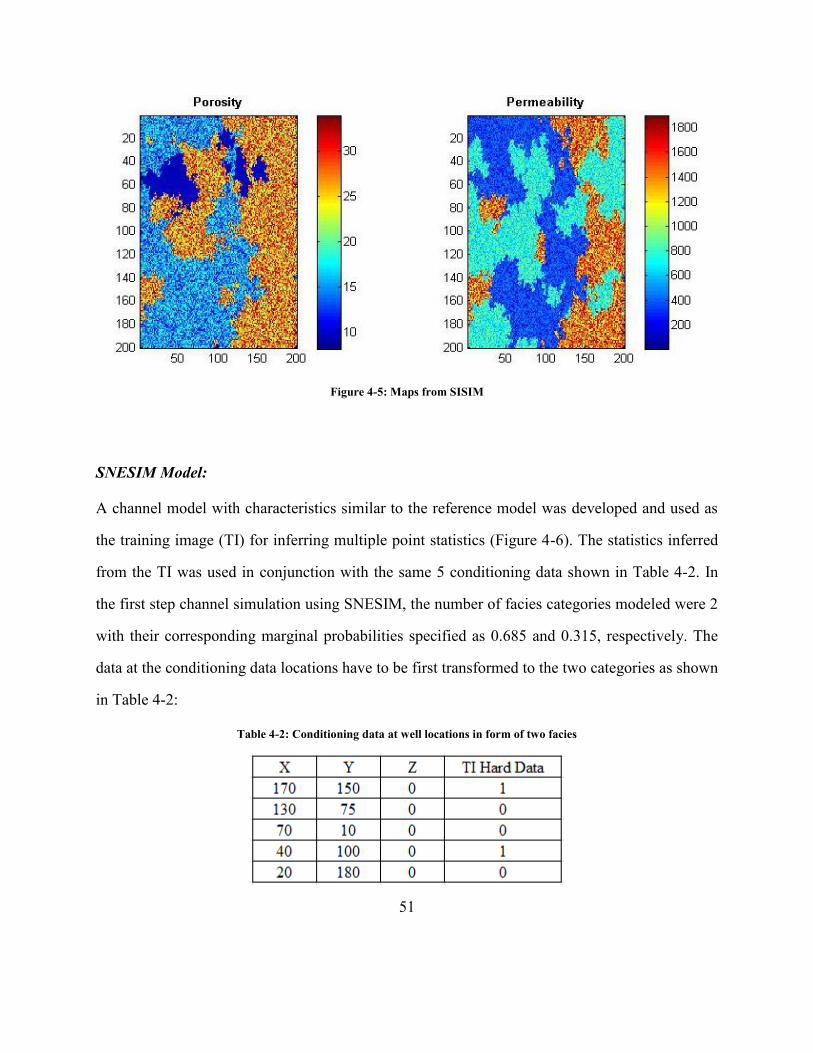
51
Figure 4-5: Maps from SISIM
SNESIM Model:
A channel model with characteristics similar to the reference model was developed and used as
the training image (TI) for inferring multiple point statistics (Figure 4-6). The statistics inferred
from the TI was used in conjunction with the same 5 conditioning data shown in Table 4-2. In
the first step channel simulation using SNESIM, the number of facies categories modeled were 2
with their corresponding marginal probabilities specified as 0.685 and 0.315, respectively. The
data at the conditioning data locations have to be first transformed to the two categories as shown
in Table 4-2:
Table 4-2: Conditioning data at well locations in form of two facies

52
Figure 4-6: TI used as input in the SNESIM program
Using the statistics inferred from the TI, threshold values along with their marginal distributions,
and conditioning hard data as input to the SNESIM program, we get 100 realizations of the
output in form of 2 facies only i.e. 0 and 1, the same number of facies that our input TI
contained. After generating the output in the form of 2 facies, we assign the permeability of the
mudstone and channel to each output of 0 and 1facies, respectively. These permeability values
were obtained by performing Gaussian simulations for each facies and finally cutting and pasting
values depending on the facies category simulated using SNESIM. Because our conjecture is that
the facies geometry has a primary control on the flow characteristics of the models, only one
realization of permeability per facies was generated and used with multiple realizations of the
facies model generated using SNESIM. This is how the gridded maps of permeability are
obtained. Porosity is obtained from the empirical relation between permeability and porosity for
the same field.
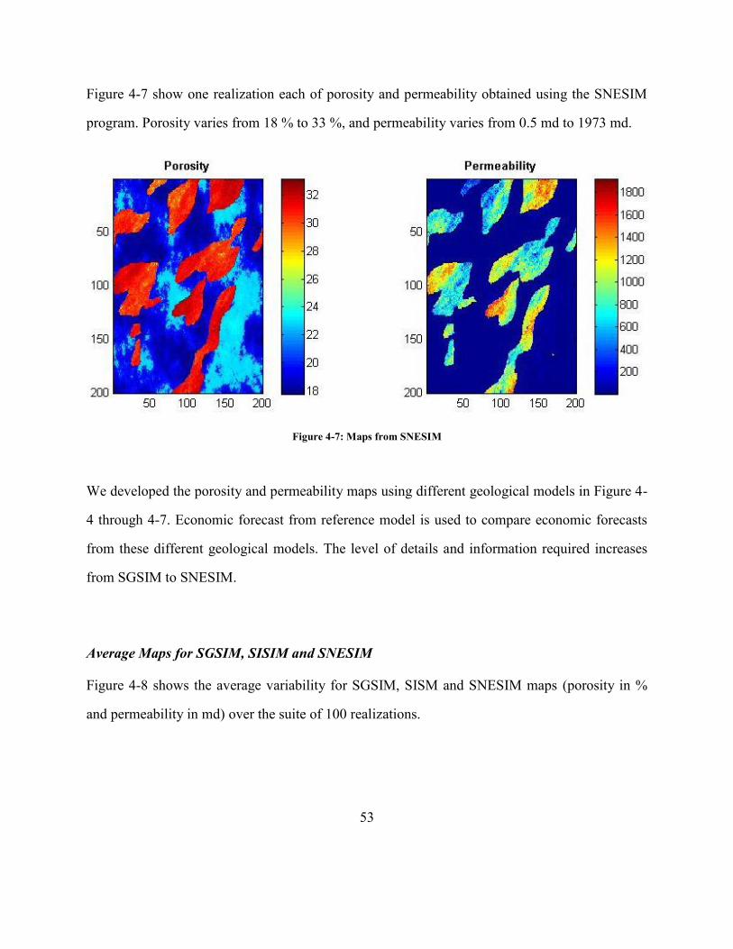
53
Figure 4-7 show one realization each of porosity and permeability obtained using the SNESIM
program. Porosity varies from 18 % to 33 %, and permeability varies from 0.5 md to 1973 md.
Figure 4-7: Maps from SNESIM
We developed the porosity and permeability maps using different geological models in Figure 4-
4 through 4-7. Economic forecast from reference model is used to compare economic forecasts
from these different geological models. The level of details and information required increases
from SGSIM to SNESIM.
Average Maps for SGSIM, SISIM and SNESIM
Figure 4-8 shows the average variability for SGSIM, SISM and SNESIM maps (porosity in %
and permeability in md) over the suite of 100 realizations.
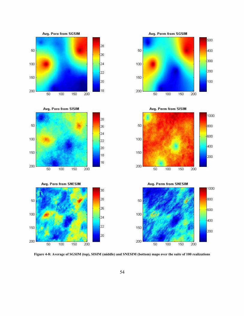
54
Figure 4-8: Average of SGSIM (top), SISIM (middle) and SNESIM (bottom) maps over the suite of 100 realizations
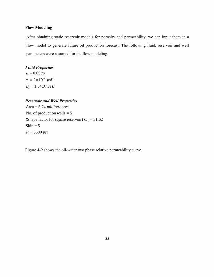
55
Flow Modeling
After obtaining static reservoir models for porosity and permeability, we can input them in a
flow model to generate future oil production forecast. The following fluid, reservoir and well
parameters were assumed for the flow modeling.
Fluid Properties
6 1
0.65
2 10
1.54 /
t
o
cp
c psi
B B STB
Reservoir and Well Properties
Area = 5.74
No. of production wells = 5
(Shape factor for square reservoir) 31.62
Skin = 5
3500
A
i
millionacres
C
P psi
Figure 4-9 shows the oil-water two phase relative permeability curve.

56
Figure 4-9: Two phase oil-water relative permeability curve assumed for the flow simulations
We input these properties and multiple realizations of the static reservoir models in the CMG to
get well flow responses corresponding to each realization. Figure 4-10 shows one of the reservoir
models gridded for flow. There are five production wells which are assumed to produce
hydrocarbons through natural water drive without any injectors. The wells are located at the
locations given in Table 4-1:
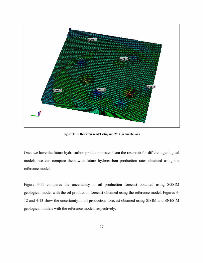
57
Figure 4-10: Reservoir model setup in CMG for simulations
Once we have the future hydrocarbon production rates from the reservoir for different geological
models, we can compare them with future hydrocarbon production rates obtained using the
reference model.
Figure 4-11 compares the uncertainty in oil production forecast obtained using SGSIM
geological model with the oil production forecast obtained using the reference model. Figures 4-
12 and 4-13 show the uncertainty in oil production forecast obtained using SISIM and SNESIM
geological models with the reference model, respectively.
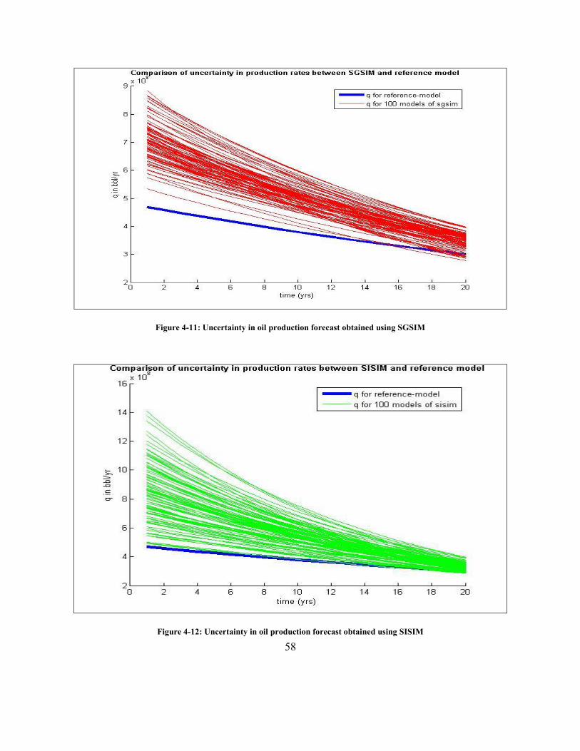
58
Figure 4-11: Uncertainty in oil production forecast obtained using SGSIM
Figure 4-12: Uncertainty in oil production forecast obtained using SISIM
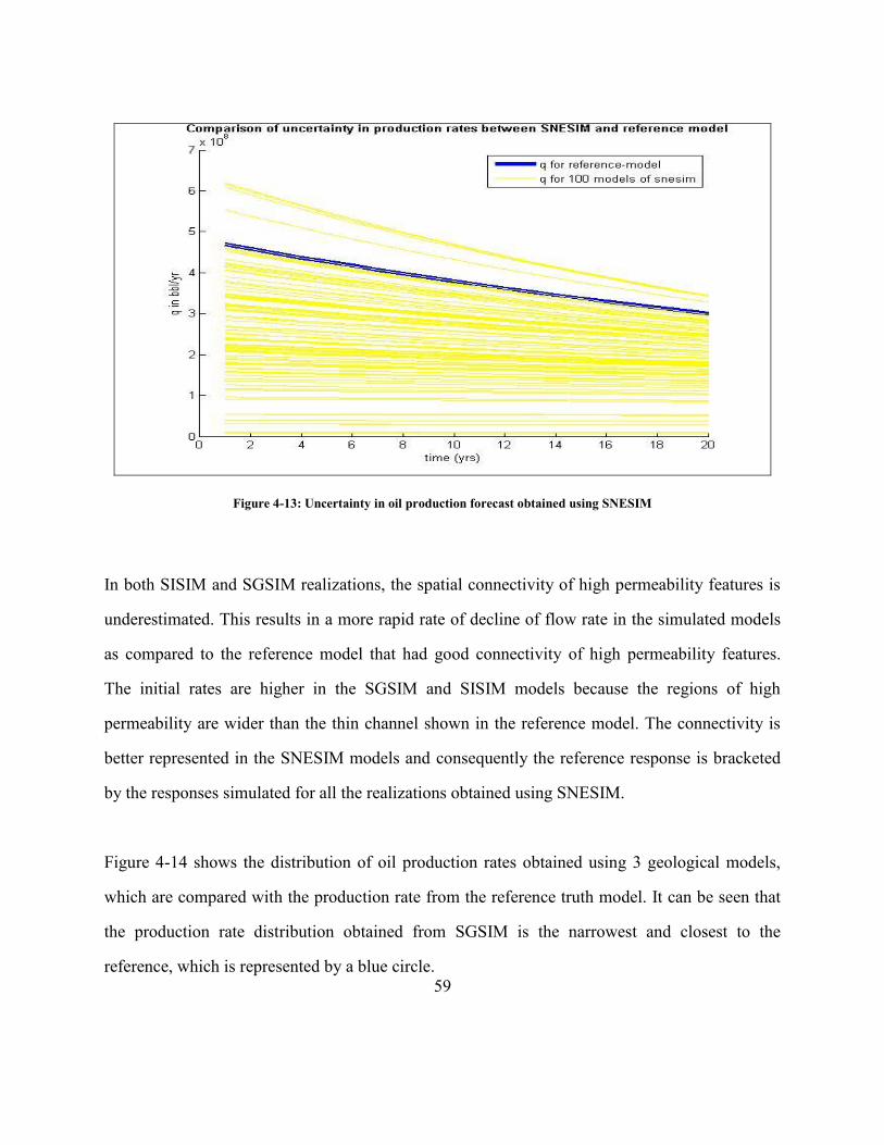
59
Figure 4-13: Uncertainty in oil production forecast obtained using SNESIM
In both SISIM and SGSIM realizations, the spatial connectivity of high permeability features is
underestimated. This results in a more rapid rate of decline of flow rate in the simulated models
as compared to the reference model that had good connectivity of high permeability features.
The initial rates are higher in the SGSIM and SISIM models because the regions of high
permeability are wider than the thin channel shown in the reference model. The connectivity is
better represented in the SNESIM models and consequently the reference response is bracketed
by the responses simulated for all the realizations obtained using SNESIM.
Figure 4-14 shows the distribution of oil production rates obtained using 3 geological models,
which are compared with the production rate from the reference truth model. It can be seen that
the production rate distribution obtained from SGSIM is the narrowest and closest to the
reference, which is represented by a blue circle.
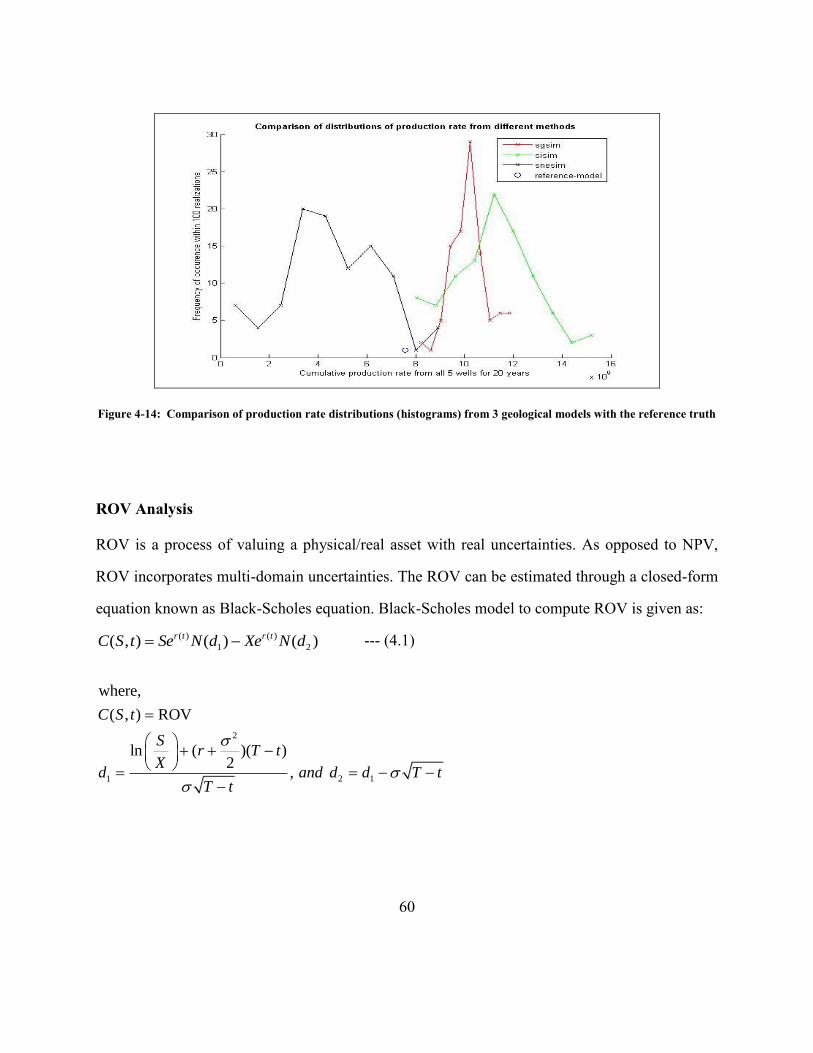
60
Figure 4-14: Comparison of production rate distributions (histograms) from 3 geological models with the reference truth
ROV Analysis
ROV is a process of valuing a physical/real asset with real uncertainties. As opposed to NPV,
ROV incorporates multi-domain uncertainties. The ROV can be estimated through a closed-form
equation known as Black-Scholes equation. Black-Scholes model to compute ROV is given as:
--- (4.1)
2
1 2 1
where,
( , ) ROV
ln ( )( )2
,
C S t
Sr T t
Xd and d d T t
T t
( ) ( )
1 2( , ) ( ) ( )r t r tC S t Se N d Xe N d
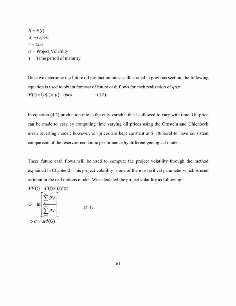
61
( )
capex
12%
Project Volatility
Time period of maturity
S F t
X
r
T
Once we determine the future oil production rates as illustrated in previous section, the following
equation is used to obtain forecast of future cash flows for each realization of q(t):
( ) ( )F t q t p opex --- (4.2)
In equation (4.2) production rate is the only variable that is allowed to vary with time. Oil price
can be made to vary by computing time varying oil prices using the Ornstein and Uhlenbeck
mean reverting model; however, oil prices are kept constant at $ 30/barrel to have consistent
comparison of the reservoir economic performance by different geological models.
These future cash flows will be used to compute the project volatility through the method
explained in Chapter 2. This project volatility is one of the most critical parameter which is used
as input in the real options model. We calculated the project volatility as following:
( ) ( ) ( )PV t F t DV t
1
0
ln
( )
n
i
i
n
i
i
PV
G
PV
std G
--- (4.3)

62
h
where,
Present value at i year
std( ) Standard deviation
Project Volatility
t
iPV
We will obtain G from equation (4.3) for every realization and, therefore, a histogram of G can
be plotted. The volatility will be the standard deviation of the distribution G.
Figure 4-15 shows the time varying project volatility‟s magnitude decreasing with time. The
reason for the decrease in project volatility with time is because there is more prior data of the
reservoir‟s economic performance (in terms of DCF). In addition to the above factor, the
volatility decreases because as fluid is produced for increased duraction the effect of geologic
uncertainty on reservoir product decreases. This is because larger volume of the reservoir is
already contacted by the injected water as time progresses.
Figure 4-15: Variation of project volatility with time for different models and reference truth
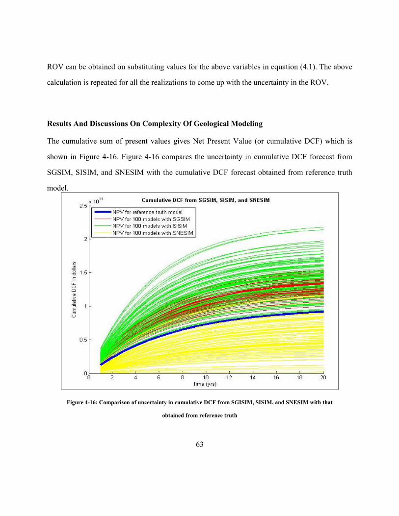
63
ROV can be obtained on substituting values for the above variables in equation (4.1). The above
calculation is repeated for all the realizations to come up with the uncertainty in the ROV.
Results And Discussions On Complexity Of Geological Modeling
The cumulative sum of present values gives Net Present Value (or cumulative DCF) which is
shown in Figure 4-16. Figure 4-16 compares the uncertainty in cumulative DCF forecast from
SGSIM, SISIM, and SNESIM with the cumulative DCF forecast obtained from reference truth
model.
Figure 4-16: Comparison of uncertainty in cumulative DCF from SGISIM, SISIM, and SNESIM with that
obtained from reference truth
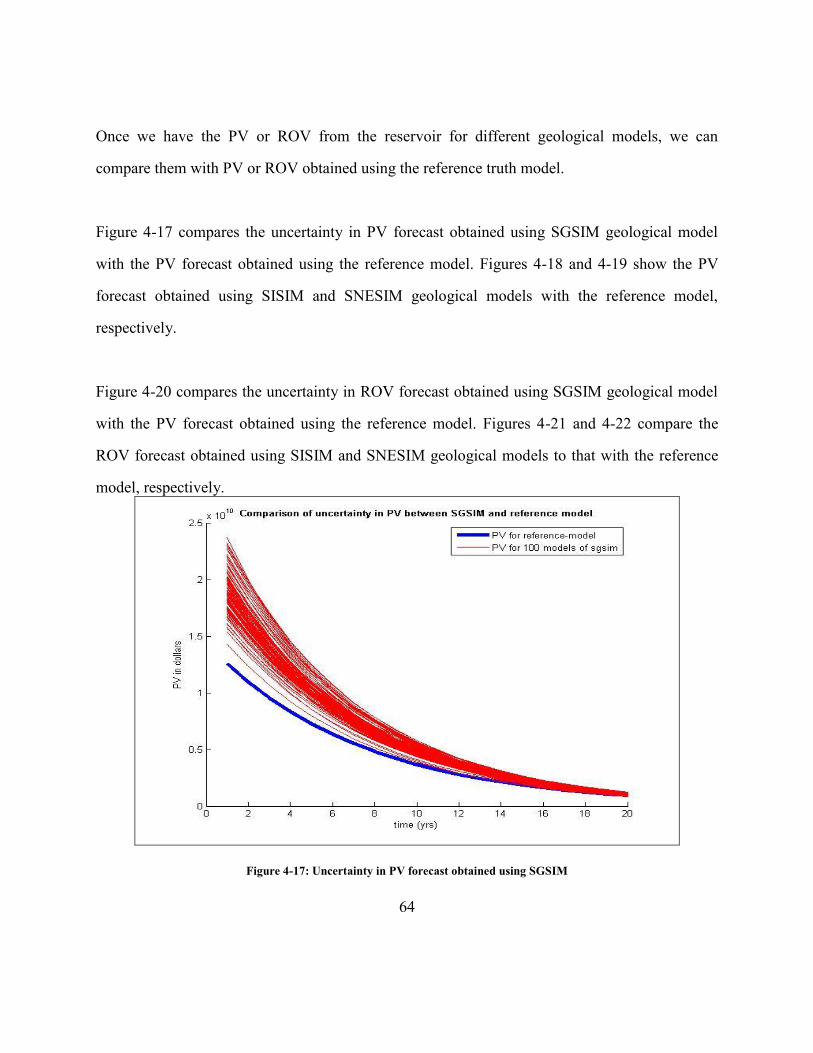
64
Once we have the PV or ROV from the reservoir for different geological models, we can
compare them with PV or ROV obtained using the reference truth model.
Figure 4-17 compares the uncertainty in PV forecast obtained using SGSIM geological model
with the PV forecast obtained using the reference model. Figures 4-18 and 4-19 show the PV
forecast obtained using SISIM and SNESIM geological models with the reference model,
respectively.
Figure 4-20 compares the uncertainty in ROV forecast obtained using SGSIM geological model
with the PV forecast obtained using the reference model. Figures 4-21 and 4-22 compare the
ROV forecast obtained using SISIM and SNESIM geological models to that with the reference
model, respectively.
Figure 4-17: Uncertainty in PV forecast obtained using SGSIM

65
Figure 4-18: Uncertainty in PV forecast obtained using SISIM
Figure 4-19: Uncertainty in PV forecast obtained using SNESIM

66
Figure 4-20: Uncertainty in ROV forecast obtained using SGSIM
Figure 4-21: Uncertainty in ROV forecast obtained using SISIM

67
Figure 4-22: Uncertainty in ROV forecast obtained using SNESIM
Therefore, it can be seen that the output of these geological models in terms of economic returns
from the reservoir does not show significant variation compared to each other. In fact it is seen
that the least complex geological model, SGSIM, matches closely with the reference.
However, if we do the ROV analysis corresponding to the mean production profile from all
different models, then the results indicate that ROV corresponding to mean production profile
from SNESIM is closest to the reference. Figures 4-23 and 4-24 show mean production histories,
and ROV corresponding to the mean production histories from all different models, respectively.
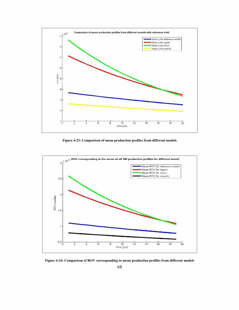
68
Figure 4-23: Comparison of mean production profiles from different models
Figure 4-24: Comparison of ROV corresponding to mean production profiles from different models
69
Overall, the initial economic returns from all the three geological models are about same with
respect to the reference, but the PV amount is in general less than the ROV throughout the life of
the reservoir. This implies that project valuation using the conventional DCF technique fails to
unearth the hidden economic potential of the project that is brought to the fore by the ROV
analysis.
ASSESSING THE IMPACT OF DETAILED FLOW MODELING
Research Approach
Similar to the preceding discussion on complexity of the geologic model, it may be useful also to
study the impact of complex flow modeling on assessing the uncertainty in flow response
characteristics and further on assessing the impact on ROV or NPV. Decline curve analysis can
be a good choice if the long term production performance prediction is the ultimate objective.
To forecast the economic performance of the reservoir, we need future hydrocarbon production
rates which can be determined using full physics commercial simulator such as CMG or decline
curve analysis. For this case study on assessing the economic implication of flow modeling
complexity, we use predicted hydrocarbon production rates from the case study in Chapter 3.
The description of the case study from Chapter 3 is briefly recounted below.
Description of the Problem
We assume a reservoir with grid dimension of 50 x 50 x 1 that initially has 5 production wells
only. The only basic information available about the reservoir characteristics such as porosity
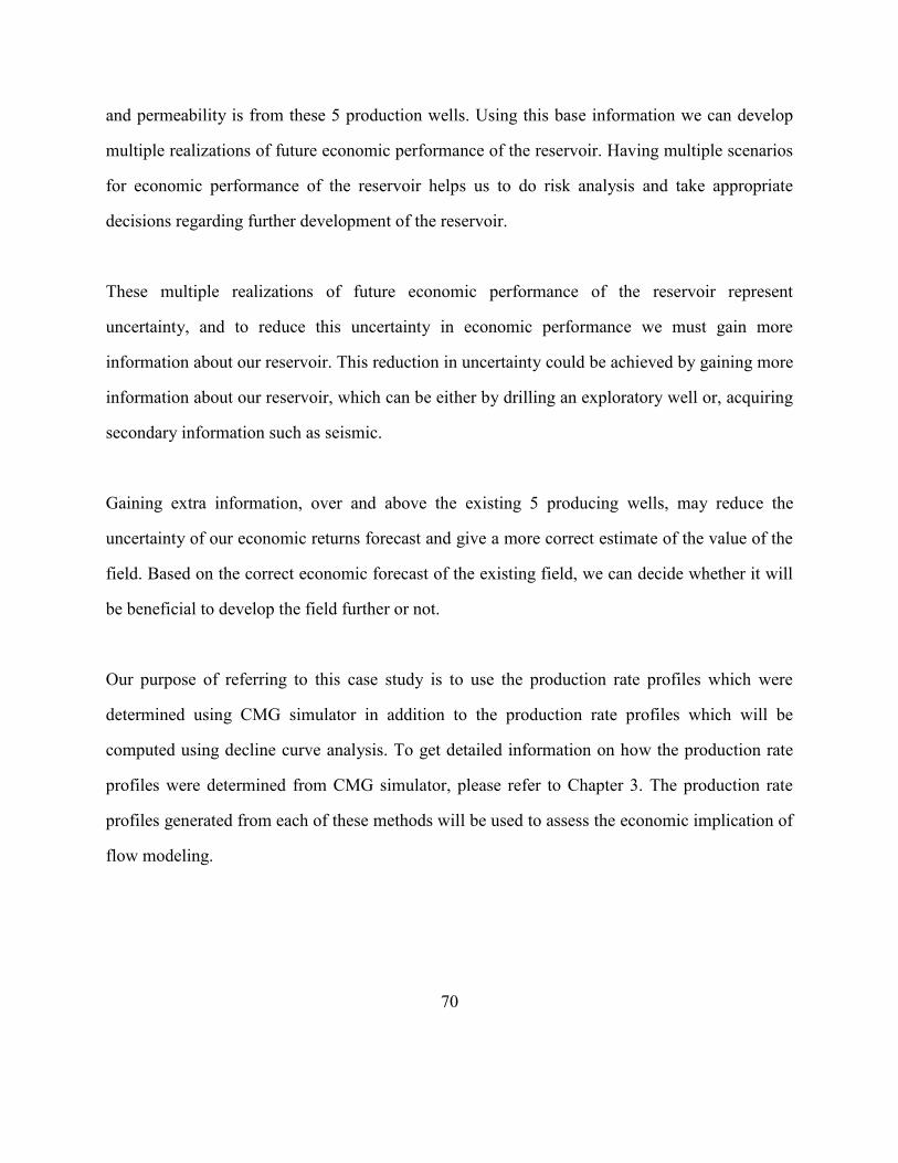
70
and permeability is from these 5 production wells. Using this base information we can develop
multiple realizations of future economic performance of the reservoir. Having multiple scenarios
for economic performance of the reservoir helps us to do risk analysis and take appropriate
decisions regarding further development of the reservoir.
These multiple realizations of future economic performance of the reservoir represent
uncertainty, and to reduce this uncertainty in economic performance we must gain more
information about our reservoir. This reduction in uncertainty could be achieved by gaining more
information about our reservoir, which can be either by drilling an exploratory well or, acquiring
secondary information such as seismic.
Gaining extra information, over and above the existing 5 producing wells, may reduce the
uncertainty of our economic returns forecast and give a more correct estimate of the value of the
field. Based on the correct economic forecast of the existing field, we can decide whether it will
be beneficial to develop the field further or not.
Our purpose of referring to this case study is to use the production rate profiles which were
determined using CMG simulator in addition to the production rate profiles which will be
computed using decline curve analysis. To get detailed information on how the production rate
profiles were determined from CMG simulator, please refer to Chapter 3. The production rate
profiles generated from each of these methods will be used to assess the economic implication of
flow modeling.

71
Decline Curve Model
Decline curve model used to predict the field‟s production rates was taken from Chapter 9 of
Walsh and Lake (2003). All the units in following formulas are expressed in oilfield units to
maintain consistency.
2
0.00708
1ln 5.75
2
o
k
w
w A
hkJ
As
r C
365 w k
p t
N J
V C
7757.792pV Ah
( )w k i wf
osci
oi
N J p pq
B
365 [1 exp( )]osci
p
qN t
0( )exp( ( ))i wf wftp p p t t p

72
where,
Well productivity index[rb/day/psi]
Shapefactor
Well radius[ft]
Reservoir thickness[ft]
Permeability relative tooil
Drainagearea[acres]
Skin factor
Decayconstant[1/year]
Number of wells
P
k
A
w
o
w
J
C
r
h
k
A
s
N
0
orosity
Pore volume[rb]
Formation volumefactor[rb/STB]
Initial producing rate[STB/day]
Cumulativeoil production[STB]
Project start time
Average pressureafter t years[psi]
Bottomhole pressure
p
oi
osci
p
t
wf
V
B
q
N
t
p
p
Flow Modeling
The cases presented here were not run in a history matching mode. In other words, once the
decline parameters were established they are not updated. We are simply trying to ascertain if the
complexity of the flow model contributes in any way to the assessment of value of information
stemming from assimilation of different types of reservoir data. Part of the problem is that we
decided to do this on a different case example than that for the rest of the chapter.

73
Figures 4-25 and 4-26 compare the uncertainty in oil production forecast determined using CMG
and decline curve analysis, respectively, for the 2 scenarios from the strategy discussed in
Chapter 3.
Figure 4-25: Uncertainty in oil production forecast determined using CMG
Figure 4-26: Uncertainty in oil production forecast determined using decline curve analysis
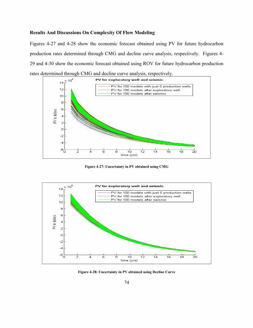
74
Results And Discussions On Complexity Of Flow Modeling
Figures 4-27 and 4-28 show the economic forecast obtained using PV for future hydrocarbon
production rates determined through CMG and decline curve analysis, respectively. Figures 4-
29 and 4-30 show the economic forecast obtained using ROV for future hydrocarbon production
rates determined through CMG and decline curve analysis, respectively.
Figure 4-27: Uncertainty in PV obtained using CMG
Figure 4-28: Uncertainty in PV obtained using Decline Curve

75
Figure 4-29: ROV obtained using CMG
Figure 4-30: ROV obtained using Decline Curve

76
A key observation, with regards to comparison of figures 4-29 and 4-30 is that the distribution of
uncertainty in ROV is reduced when using the decline curve. This is to be expected since the
entire spatial variability exhibited by porosity and permeability as depicted over the suite of
realizations is reduced to a single effective value that is input into the decline curve model. We
can see from the above figures that the results from decline curve analysis, for the economic
returns from the reservoir over its life period of 20 years, match quite well with the results from a
commercial simulator CMG.
There is a raging debate within the modeling (reservoir, flow and economic) community on the
worth of producing sophisticated models that exhibit physical realism. This study explores this
issue using economic measures such as PV and ROV. Preliminary results that might be specific
to the case study set up in this study seem to indicate that complexity in models might not always
translate to improved accuracies in economic forecasts. In fact, project volatility derived using
several realizations of the geological model might often dwarf uncertainty in flow performance
modeled using sophisticated schemes.

77
Chapter 5: Binomial-Lattice Option Valuation
INTRODUCTION
Traditional discounted cash flow (DCF) methods of valuation fail to account for the value of
managerial flexibility present in many types of projects. For example, NPV analysis does not
capture the effects of decision to expand or abandon the project. The real options valuation, a
stochastic approach, is a method to value capital investment projects that involve managerial
flexibilities (Dixit & Pindyck 1995).
The concept and theory of Real Options is explained in Chapter 2. We also show in Chapter 3
and 4 the utility of real options using Black-Scholes model to discover hidden value in modeling
and data acquisition decisions that would not have been evident using conventional DCF
analysis.
The main drawback of using the Black-Scholes model is that the Black-Scholes equation is a
solution to a stochastic differential equation corresponding to a set of restrictive assumptions.
The Binomial lattice on the other hand permits the evaluation of projects that may not follow the
strict prescription of initial and boundary conditions specified as part of the Black-Scholes
solution.
Binomial Lattice Option Valuation (BLOV) is a generalized numerical method for the valuation
of options. In general, the BLOV model does not have closed-form solutions (Cox et al. 1979).
Although BLOV is computationally slower than the Black-Scholes model for ROV, it is more
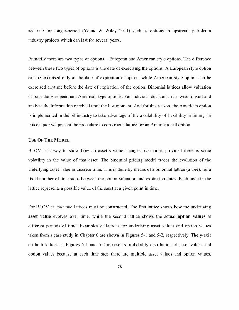
78
accurate for longer-period (Yound & Wiley 2011) such as options in upstream petroleum
industry projects which can last for several years.
Primarily there are two types of options – European and American style options. The difference
between these two types of options is the date of exercising the options. A European style option
can be exercised only at the date of expiration of option, while American style option can be
exercised anytime before the date of expiration of the option. Binomial lattices allow valuation
of both the European and American-type options. For judicious decisions, it is wise to wait and
analyze the information received until the last moment. And for this reason, the American option
is implemented in the oil industry to take advantage of the availability of flexibility in timing. In
this chapter we present the procedure to construct a lattice for an American call option.
USE OF THE MODEL
BLOV is a way to show how an asset‟s value changes over time, provided there is some
volatility in the value of that asset. The binomial pricing model traces the evolution of the
underlying asset value in discrete-time. This is done by means of a binomial lattice (a tree), for a
fixed number of time steps between the option valuation and expiration dates. Each node in the
lattice represents a possible value of the asset at a given point in time.
For BLOV at least two lattices must be constructed. The first lattice shows how the underlying
asset value evolves over time, while the second lattice shows the actual option values at
different periods of time. Examples of lattices for underlying asset values and option values
taken from a case study in Chapter 6 are shown in Figures 5-1 and 5-2, respectively. The y-axis
on both lattices in Figures 5-1 and 5-2 represents probability distribution of asset values and
option values because at each time step there are multiple asset values and option values,
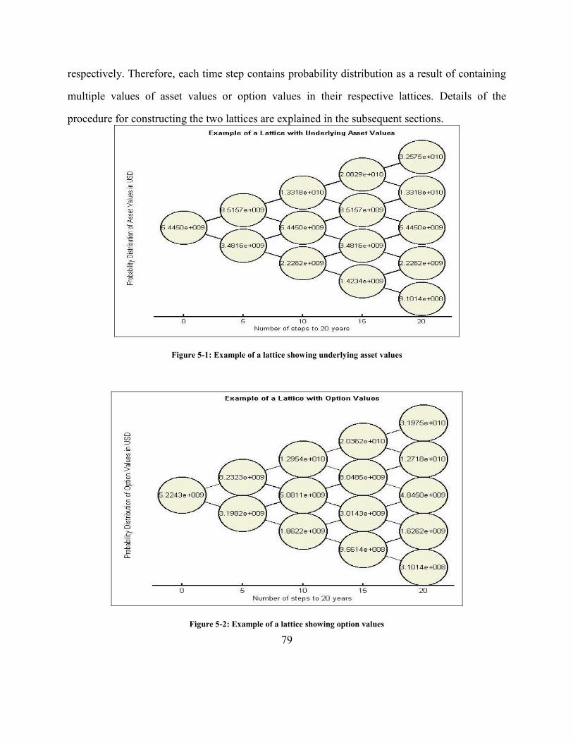
79
respectively. Therefore, each time step contains probability distribution as a result of containing
multiple values of asset values or option values in their respective lattices. Details of the
procedure for constructing the two lattices are explained in the subsequent sections.
Figure 5-1: Example of a lattice showing underlying asset values
Figure 5-2: Example of a lattice showing option values
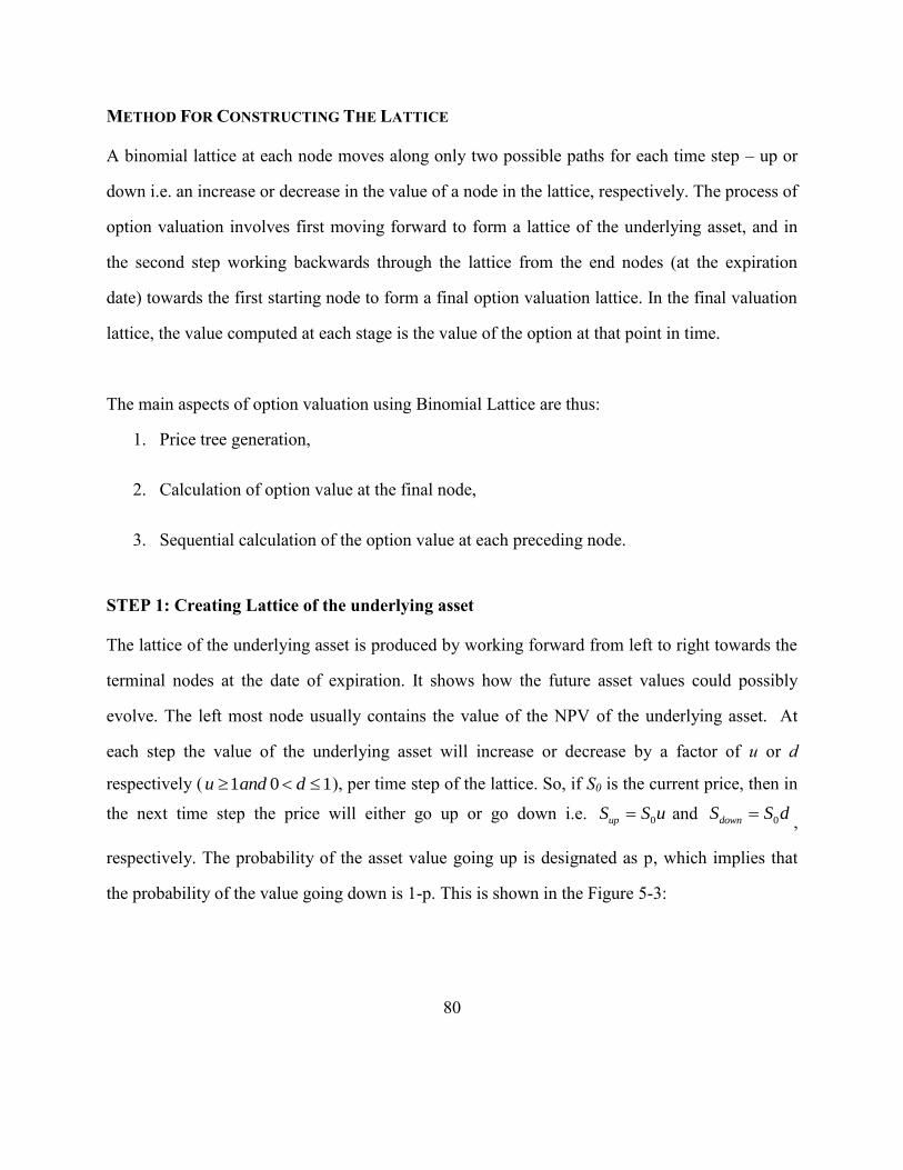
80
METHOD FOR CONSTRUCTING THE LATTICE
A binomial lattice at each node moves along only two possible paths for each time step – up or
down i.e. an increase or decrease in the value of a node in the lattice, respectively. The process of
option valuation involves first moving forward to form a lattice of the underlying asset, and in
the second step working backwards through the lattice from the end nodes (at the expiration
date) towards the first starting node to form a final option valuation lattice. In the final valuation
lattice, the value computed at each stage is the value of the option at that point in time.
The main aspects of option valuation using Binomial Lattice are thus:
1. Price tree generation,
2. Calculation of option value at the final node,
3. Sequential calculation of the option value at each preceding node.
STEP 1: Creating Lattice of the underlying asset
The lattice of the underlying asset is produced by working forward from left to right towards the
terminal nodes at the date of expiration. It shows how the future asset values could possibly
evolve. The left most node usually contains the value of the NPV of the underlying asset. At
each step the value of the underlying asset will increase or decrease by a factor of u or d
respectively ( 1 0 1u and d ), per time step of the lattice. So, if S0 is the current price, then in
the next time step the price will either go up or go down i.e. 0upS S u and 0downS S d,
respectively. The probability of the asset value going up is designated as p, which implies that
the probability of the value going down is 1-p. This is shown in the Figure 5-3:

81
Figure 5-3: Construction of lattice for an underlying asset illustrating the process of construction of lattice for an
underlying asset. The value of the asset is first constructed by going from left to right. Subsequently, the option value is
computed by traversing the lattice from right to left.
We‟ll need the probability p in Step 2 below where we‟ll talk more about it, and also derive its
formula. The factors u and d, which determine the upward and downward movements at each
node, are functions of the volatility of the underlying asset and the time step between each
column of the lattice. They are given as:
1t tu e and d eu
is the project volatility. The derivation of these expressions for u and d is presented in a
subsequent section.
If we repeat this method of filling up the nodes at different time steps, a lattice will evolve as
shown in the Figure 5-4. The probability distribution shown in the right side of Figure 5-4 is
obtained from asset values in the terminal nodes of the lattice and the spread of that distribution
will be controlled by the project volatility (Bailey et al. 2003). This resultant lattice in Figure 5-4
is called as the lattice of the underlying asset.
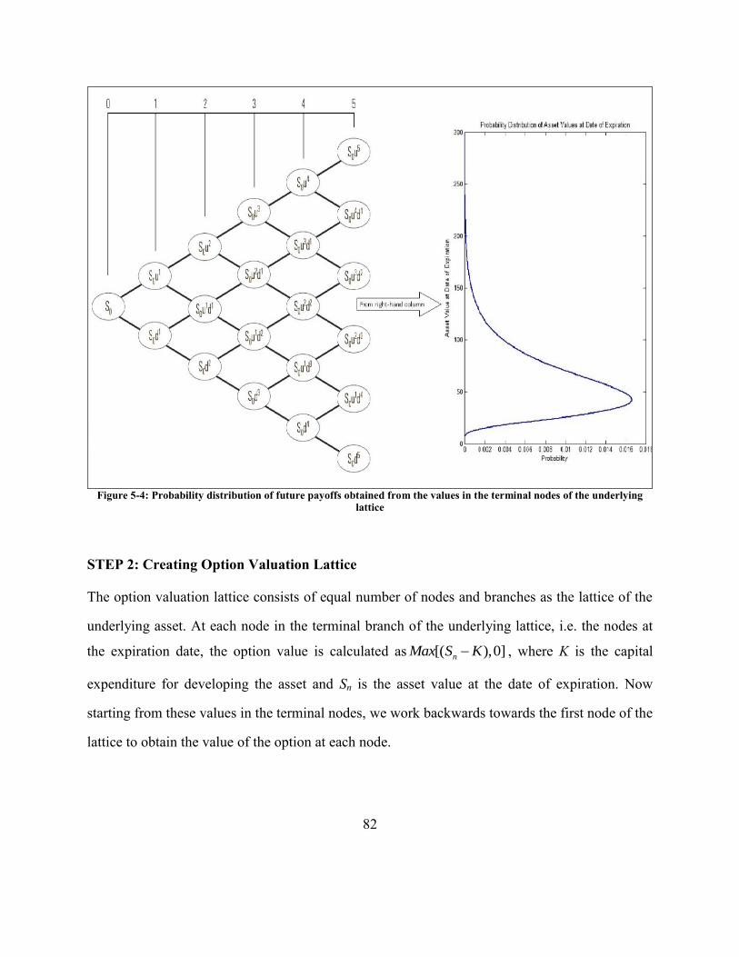
82
Figure 5-4: Probability distribution of future payoffs obtained from the values in the terminal nodes of the underlying
lattice
STEP 2: Creating Option Valuation Lattice
The option valuation lattice consists of equal number of nodes and branches as the lattice of the
underlying asset. At each node in the terminal branch of the underlying lattice, i.e. the nodes at
the expiration date, the option value is calculated as [( ),0]nMax S K , where K is the capital
expenditure for developing the asset and Sn is the asset value at the date of expiration. Now
starting from these values in the terminal nodes, we work backwards towards the first node of the
lattice to obtain the value of the option at each node.
83
Derivation for p, u and d
We start with a condition of the Black-Scholes model whereby we want to match the mean and
variance, i.e. moments, of the returns of S in our lattice to the mean and variance in the real
world.
In a risk neutral world, the expected gross return after a time ∆t is er△ t
, where r is the risk free
rate. As per the risk neutrality assumption, the value of an asset at today‟s date is equal to the
expected value of its future payoff discounted by the risk free rate i.e.
0
0
,t r tt
r t
E S SS or E e
Se
--- (5.1)
Where, 0S is the value of an asset at today‟s date, and tS is the future payoff at time ∆t.
Because u and d are the gross returns of S0 and the mean gross return is er△ t
, therefore we must
also have:
(1 ) r tpu p d e --- (5.2)
Combining Equation (5.2) with (5.1), we have:
0
(1 )tSE pu p d
S
0 (1 )tE S S pu p d
Therefore, the variance will be:
2 2
2 2
0 0 0
2 2 2 2 2
0 02
0
1 1( ) ( ) [ ( )]
1[ (1 ) ] [ (1 ) ]
tt t t
SVar Var S E S E S
S S S
S pu p d S pu p dS
84
2 2 2
0
[ (1 ) ] [ (1 ) ]tSVar pu p d pu p d
S
--- (5.3)
Substituting Eq. (5.2) in Eq. (5.3):
2 2 2
0
[ (1 ) ] ttSVar pu p d e
S
--- (5.3A)
In the Black-Scholes model we have a lognormally distributed asset value with variance as: 2 22 2 2 2 2
0 0( ) ( 1) ( )r t t r t t r t
tVar S S e e S e e
22 2
0
( )r t t r ttSVar e e
S
--- (5.4)
Equating the right side of Equations 5.3A and 5.4, we obtain: 22 2 2(1 ) r t tpu p d e --- (5.5)
To infer the parameters of our lattice p, u and d we need one more equation in addition to
Equations (5.2) and (5.5). Different authors have introduced different constraints to obtain a
solution. The best known solution is obtained by the constrained introduced by Cox et al. (Cox et
al. 1979) for asymmetric asset appreciation and decline which we used above in step 1:
1ud --- (5.6)
Using Equations (5.2), (5.5) and (5.6), we obtain: r te d
pu d
1t tu e and d eu
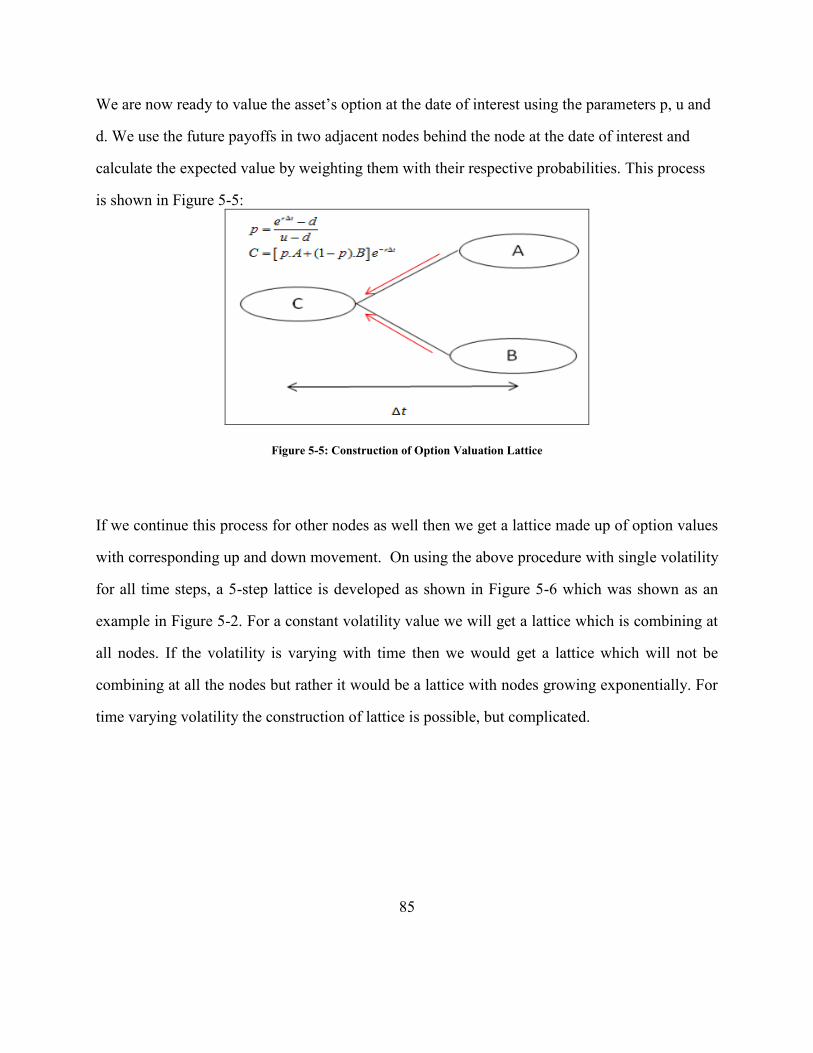
85
We are now ready to value the asset‟s option at the date of interest using the parameters p, u and
d. We use the future payoffs in two adjacent nodes behind the node at the date of interest and
calculate the expected value by weighting them with their respective probabilities. This process
is shown in Figure 5-5:
Figure 5-5: Construction of Option Valuation Lattice
If we continue this process for other nodes as well then we get a lattice made up of option values
with corresponding up and down movement. On using the above procedure with single volatility
for all time steps, a 5-step lattice is developed as shown in Figure 5-6 which was shown as an
example in Figure 5-2. For a constant volatility value we will get a lattice which is combining at
all nodes. If the volatility is varying with time then we would get a lattice which will not be
combining at all the nodes but rather it would be a lattice with nodes growing exponentially. For
time varying volatility the construction of lattice is possible, but complicated.
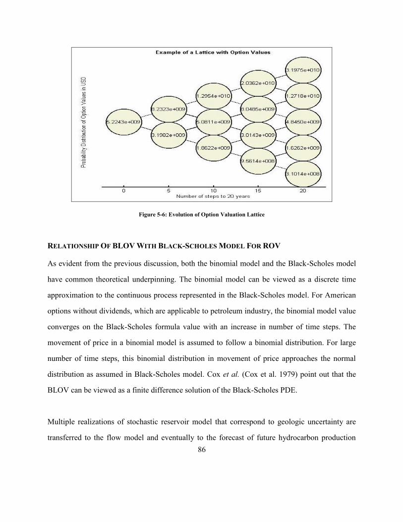
86
Figure 5-6: Evolution of Option Valuation Lattice
RELATIONSHIP OF BLOV WITH BLACK-SCHOLES MODEL FOR ROV
As evident from the previous discussion, both the binomial model and the Black-Scholes model
have common theoretical underpinning. The binomial model can be viewed as a discrete time
approximation to the continuous process represented in the Black-Scholes model. For American
options without dividends, which are applicable to petroleum industry, the binomial model value
converges on the Black-Scholes formula value with an increase in number of time steps. The
movement of price in a binomial model is assumed to follow a binomial distribution. For large
number of time steps, this binomial distribution in movement of price approaches the normal
distribution as assumed in Black-Scholes model. Cox et al. (Cox et al. 1979) point out that the
BLOV can be viewed as a finite difference solution of the Black-Scholes PDE.
Multiple realizations of stochastic reservoir model that correspond to geologic uncertainty are
transferred to the flow model and eventually to the forecast of future hydrocarbon production

87
rates. Future cash flows are function of future hydrocarbon production rates and, therefore, any
variation in future hydrocarbon production rates will result in a variation in the future cash flow
stream. Variation in future cash flows is a source of project volatility; hence, the project
volatility is also indirectly a function of volumetric flow rate uncertainty (which is related to
geologic uncertainty) because future cash flows are a direct function of volumetric flow rate.
Chapter 6 applies the framework of BLOV to analyze the economic prospects of an
undeveloped, but discovered field.
88
Chapter 6: Analyzing the Prospects of an Undeveloped Field
INTRODUCTION
This chapter explains in a simple way the application of Binomial Lattice Option Valuation
(BLOV) to the valuation of an undeveloped oil reserve. As we discussed earlier that Binomial
Lattice Option Valuation (BLOV) (Cox et al. 1979) is a generalized numerical method for the
valuation of options. Although its solution is computationally slower than the Black-Scholes
formula, it is more accurate, particularly for longer-period options such as those in upstream
petroleum industry.
The case example presented in this chapter focuses on the analysis of the reserves of an
undeveloped, but discovered, field. The future economic prospects from the field will give an
idea of how much a company may want to invest to develop the field. In this case we do the
evaluation based on recoverable reserves. Recoverable reserves are the technically and
economically recoverable portion of oil volume in the reservoir. To determine recoverable
reserves we must first evaluate original oil in place (OOIP), which is defined as the total
hydrocarbon content of an oil reservoir. It is often abbreviated as STOOIP, which stands for
stock tank original oil in place, or STOIIP for Stock Tank Oil Initially In Place, referring to the
oil in place before the commencement of production (Energy Information Administration - EIA
2008). Recovery factors for oil fields typically range between 10 and 60 percent. The wide
variance is because of the different characteristics of fluid and reservoir properties for different
deposits (Energy Information Administration - EIA 2008). By applying the estimate for recovery
factor of a field on the OOIP, we can determine the recoverable reserves.

89
DESCRIPTION OF THE PROBLEM
In the initial phase the only information the company has is sparse data that can be used to
develop the model for a reservoir. We use that initial model to do our initial economic valuation
using the binomial lattice. Once we have done the economic valuation for the potential reservoir,
by using only the initial representation, we will have two options following that economic
valuation. The first option is to accept the valuation as is that we computed by using only the
initial reservoir model without secondary information. The second option would be to invest
money for acquiring new information in the form of 3-D seismic, which can be used together
with the initial data to generate new model(s) for the reservoir, and then redo the economic
valuation for the reservoir based on the new information. Acquiring additional seismic data will
require investment. The objective is to evaluate the option of acquiring additional seismic data in
terms of uncertainty reduction over the existing model. We perform this evaluation, by
computing the real options valuation (ROV) without and with additional seismic data and use the
difference between these numbers to establish the maximum capital expenditure permissible for
seismic acquisition, for the project to be still economically viable.
MODELING APPROACH
In the initial stage of reservoir forecasting, only the reference data from 5 wells is available for
modeling. The reservoir is represented with a simulation grid dimension of 50 x 50 x 1. Using
the reference data we can develop porosity maps of the reservoir by geostatistical techniques. To
represent uncertainty we use multiple realizations of the porosity models. For the case example
presented in this chapter, we use window average of porosity models to mimic a seismic-like
attribute. The value of water saturation is found to be 15% as output from reservoir simulation
90
and it remains almost constant during the twenty year production period of the field. Using the
porosity and water saturation data we can find the OOIP as:
3
(1 )6.2898
Where,
STOIIP (stb)
Bulk volumeof the rock(m )
Porosity
Water saturation
Formation volumefactor
b w
oi
b
w
oi
V SN
B
N
V
S
B
Using an approximate estimate of the irreducible water saturation based on the type of reservoir,
we find the recovery factor of the reservoir from following relation:
1
Where,
Recovery factor
Irreducible water saturation
w wir
f
wir
f
wir
S SR
S
R
S
For this to work we need the average water saturation Sw through the life of the reservoir and so
the recovery factor will change with time. Water saturation is computed by running an analog
simulation model for the similar field. However, the change in water saturation is quite
insignificant over the time period of recovery in which case the recovery factor does not change
significantly.
Once we know the recovery factor and STOOIP the recoverable reserves from the reservoir are
simply the product of both these two parameters.
Recoverable Reserve fR N
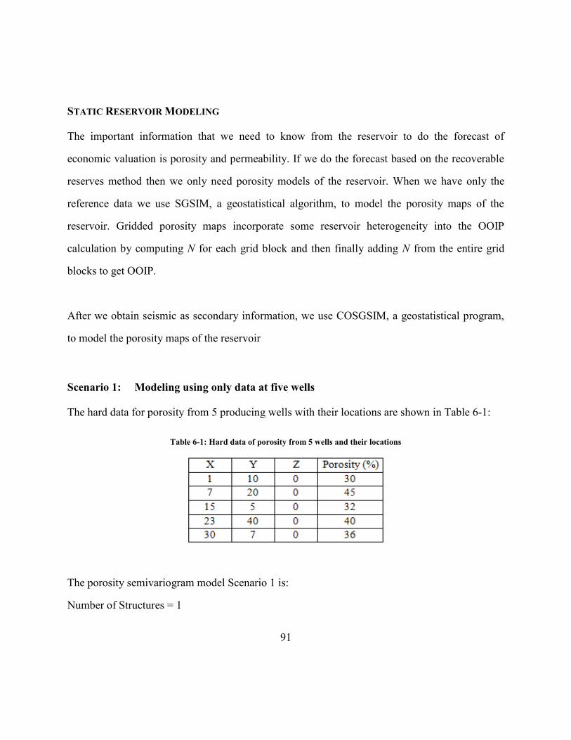
91
STATIC RESERVOIR MODELING
The important information that we need to know from the reservoir to do the forecast of
economic valuation is porosity and permeability. If we do the forecast based on the recoverable
reserves method then we only need porosity models of the reservoir. When we have only the
reference data we use SGSIM, a geostatistical algorithm, to model the porosity maps of the
reservoir. Gridded porosity maps incorporate some reservoir heterogeneity into the OOIP
calculation by computing N for each grid block and then finally adding N from the entire grid
blocks to get OOIP.
After we obtain seismic as secondary information, we use COSGSIM, a geostatistical program,
to model the porosity maps of the reservoir
Scenario 1: Modeling using only data at five wells
The hard data for porosity from 5 producing wells with their locations are shown in Table 6-1:
Table 6-1: Hard data of porosity from 5 wells and their locations
The porosity semivariogram model Scenario 1 is:
Number of Structures = 1

92
Type = Spherical
Nugget Effect = 0
Max., medium, and min. range = 1000, 100, and 20 units
Azimuth = 45 degrees
Dip = 0
Rake = 0
To obtain multiple realizations of porosity maps, hard data of porosity and variogram model for
porosity are used as input in the sequential Gaussian simulation (SGSIM) geostastical program
(Deutsch & Journel 1997). This simulation reproduces the histogram of the hard data, and honors
spatial variability of the property (variogram).
Figure 6-1 shows one of the porosity models for reference data with 5 wells whose positions are
shown as black dots:
Figure 6-1: Porosity with reference data only

93
Scenario 2: Well data and Seismic
The primary data for porosity is the data at the five well locations. We generate secondary data
which mimics seismic by taking the window average of any single porosity model that was
developed under Scenario 1. Figure 6-2 shows a smoothed map which was used as seismic data:
Figure 6-2: Seismic map on a 50 x 50 x 1 grid scale
To obtain multiple realizations of porosity maps after conditioning extra information through
secondary information which mimics seismic, primary hard data of porosity and secondary
seismic data along with variogram model for porosity are used as input in COSGSIM
geostatistical program (Xu et al., 1992) (Xu et al. 1992). The correlation between primary and
secondary variables was assumed to be 0.6. A Markov model was assumed for the co-simulation.
Under this Markov assumption, only the variogram of the primary variable is required. The
cross-variogram between the primary and secondary data is then proportional to the primary
variogram with a scaling function that is related to the correlation coefficient between the
primary and secondary variable (Xu et al. 1992).
The porosity variogram model for Scenario 2 is similar to the variogram model for Scenario 1.

94
Figure 6-3 shows one of the porosity models after integrating the seismic information with the
reference data. The black dots represent the position of the 5 wells, which act as the primary or
“hard” data.
Figure 6-3: Porosity with reference data and seismic
NPV DISTRIBUTION FORECAST
In earlier section we described how to determine recoverable reserves from the reservoir. Using
those recoverable reserves and price of oil (constant value of $70/barrel) we can estimate the Net
Present Value (NPV) from the reservoir as follow:
NPV(in $) = Recoverable Reserve (in bbl) Price of oil (in $/bbl)
By using multiple realizations of the porosity models we obtain as many NPV values as there are
porosity models. Thus, we can find P10, P25, P50, P75, and P90 from the distribution of NPV
values. Figure 6-4a and 6-4b show the histogram of the NPV values corresponding to scenario 1
and scenario 2, respectively. The NPV distribution consists of possible economic values before
we start producing from the field i.e. economic value of oil reserves that have been discovered
but not yet developed.
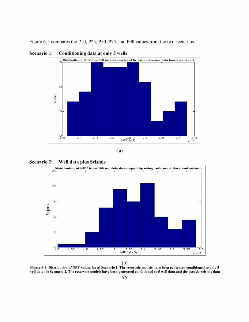
95
Figure 6-5 compares the P10, P25, P50, P75, and P90 values from the two scenarios.
Scenario 1: Conditioning data at only 5 wells
(a)
Scenario 2: Well data plus Seismic
(b) Figure 6-4: Distribution of NPV values for a) Scenario 1. The reservoir models have been generated conditioned to only 5 well data; b) Scenario 2. The reservoir models have been generated conditioned to 5 well data and the pseudo-seismic data
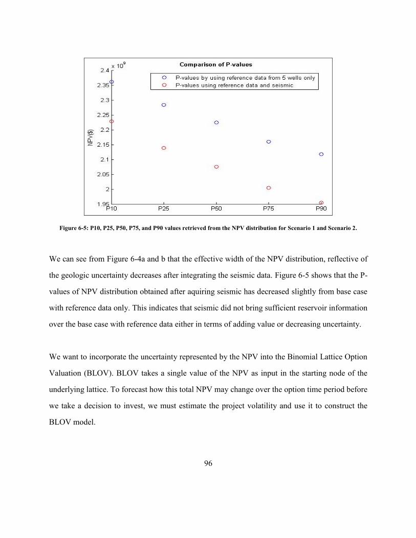
96
Figure 6-5: P10, P25, P50, P75, and P90 values retrieved from the NPV distribution for Scenario 1 and Scenario 2.
We can see from Figure 6-4a and b that the effective width of the NPV distribution, reflective of
the geologic uncertainty decreases after integrating the seismic data. Figure 6-5 shows that the P-
values of NPV distribution obtained after aquiring seismic has decreased slightly from base case
with reference data only. This indicates that seismic did not bring sufficient reservoir information
over the base case with reference data either in terms of adding value or decreasing uncertainty.
We want to incorporate the uncertainty represented by the NPV into the Binomial Lattice Option
Valuation (BLOV). BLOV takes a single value of the NPV as input in the starting node of the
underlying lattice. To forecast how this total NPV may change over the option time period before
we take a decision to invest, we must estimate the project volatility and use it to construct the
BLOV model.
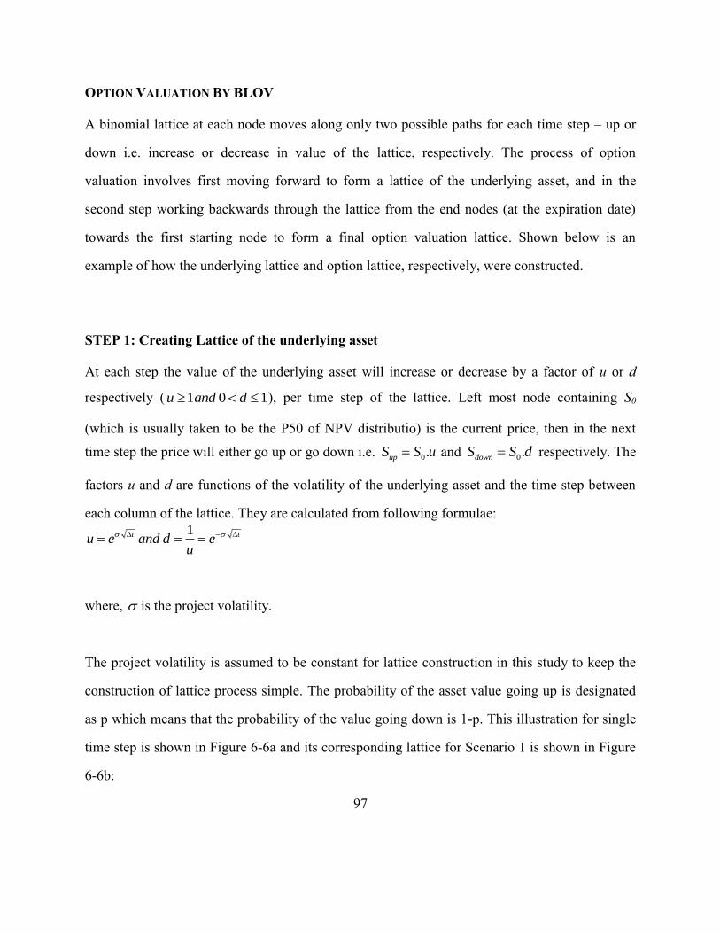
97
OPTION VALUATION BY BLOV
A binomial lattice at each node moves along only two possible paths for each time step – up or
down i.e. increase or decrease in value of the lattice, respectively. The process of option
valuation involves first moving forward to form a lattice of the underlying asset, and in the
second step working backwards through the lattice from the end nodes (at the expiration date)
towards the first starting node to form a final option valuation lattice. Shown below is an
example of how the underlying lattice and option lattice, respectively, were constructed.
STEP 1: Creating Lattice of the underlying asset
At each step the value of the underlying asset will increase or decrease by a factor of u or d
respectively ( 1 0 1u and d ), per time step of the lattice. Left most node containing S0
(which is usually taken to be the P50 of NPV distributio) is the current price, then in the next
time step the price will either go up or go down i.e. 0.upS S u and 0.downS S d respectively. The
factors u and d are functions of the volatility of the underlying asset and the time step between
each column of the lattice. They are calculated from following formulae:
1t tu e and d eu
where, is the project volatility.
The project volatility is assumed to be constant for lattice construction in this study to keep the
construction of lattice process simple. The probability of the asset value going up is designated
as p which means that the probability of the value going down is 1-p. This illustration for single
time step is shown in Figure 6-6a and its corresponding lattice for Scenario 1 is shown in Figure
6-6b:
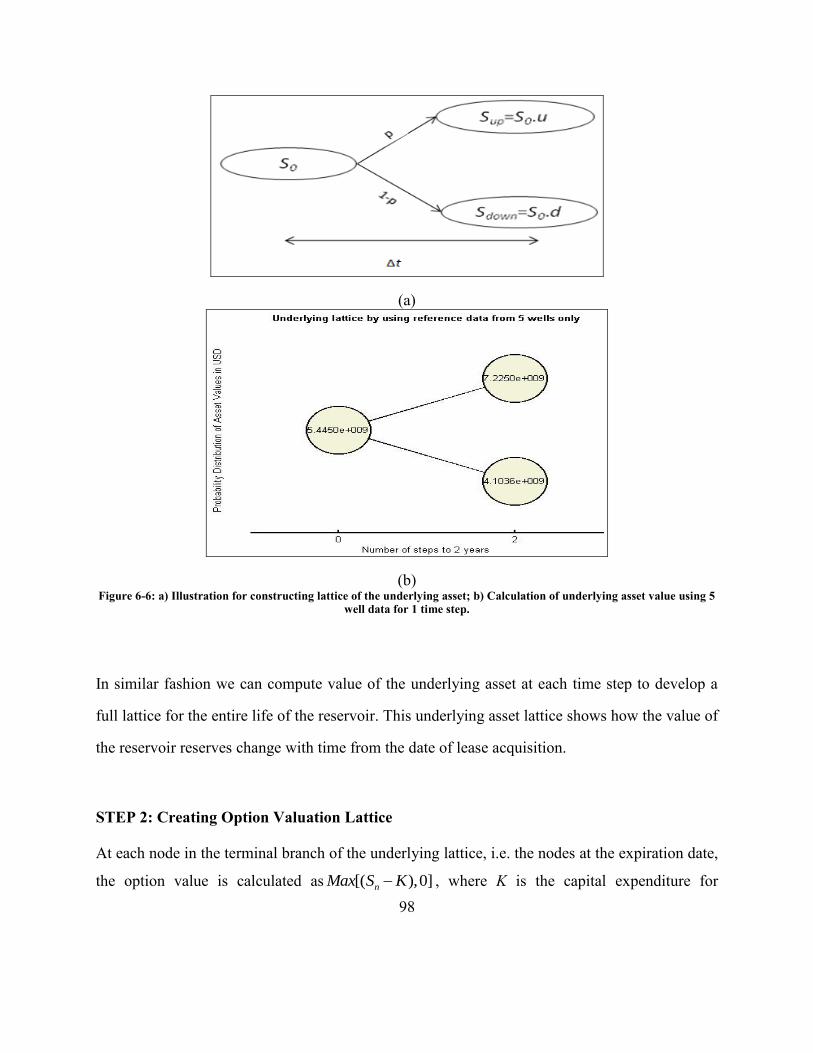
98
(a)
(b) Figure 6-6: a) Illustration for constructing lattice of the underlying asset; b) Calculation of underlying asset value using 5
well data for 1 time step.
In similar fashion we can compute value of the underlying asset at each time step to develop a
full lattice for the entire life of the reservoir. This underlying asset lattice shows how the value of
the reservoir reserves change with time from the date of lease acquisition.
STEP 2: Creating Option Valuation Lattice
At each node in the terminal branch of the underlying lattice, i.e. the nodes at the expiration date,
the option value is calculated as [( ),0]nMax S K , where K is the capital expenditure for
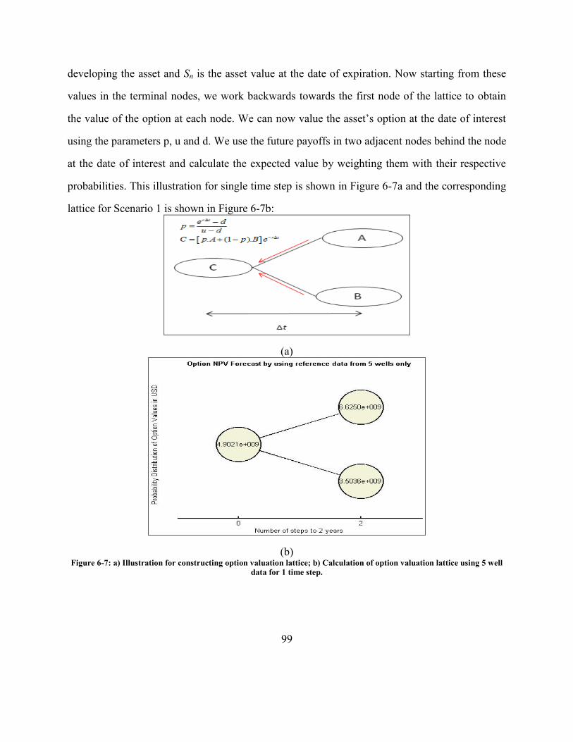
99
developing the asset and Sn is the asset value at the date of expiration. Now starting from these
values in the terminal nodes, we work backwards towards the first node of the lattice to obtain
the value of the option at each node. We can now value the asset‟s option at the date of interest
using the parameters p, u and d. We use the future payoffs in two adjacent nodes behind the node
at the date of interest and calculate the expected value by weighting them with their respective
probabilities. This illustration for single time step is shown in Figure 6-7a and the corresponding
lattice for Scenario 1 is shown in Figure 6-7b:
(a)
(b) Figure 6-7: a) Illustration for constructing option valuation lattice; b) Calculation of option valuation lattice using 5 well
data for 1 time step.

100
In similar fashion we can compute option valuation lattice at each time step to develop a full
lattice for entire life of the reservoir. It can be seen the difference in values of underlying lattice
and option lattice which occurs because of the capital expenditure ( ~ $600 million) subtracted
from the underlying asset values at the terminal nodes and then exercising backward induction.
In this particular case study the revenue is much greater than the expenditure because the
revenue is based on original oil in place for the entire field which in this case is quite large while
the expenditure is considered for drilling only 5 wells.
The option lattice shows the distribution of option values, at each time step, to develop the
reservoir. The option value corresponding to the undeveloped reservoir is shown in the left most
node of the underlying asset‟s lattice. We can value the option at the end of the lattice starting
from year 20 and doing backward induction using risk-neutral binomial option valuation. Under
risk neutrality assumption the invester is indifferent to the risk involved and is only interested in
expected value which is calculated from later two nodes as shown in Figure 6-7a. The
management can either accept an option value at some point to develop the reservoir based on
the information they have, or they can decide to opt for further information which will require
investment and base their decision on option analysis done with the new information. We have
presented two scenarios for data acquisition for improving the reservoir model. For both the
scenarios at the termination of the project (year 20), the value of the option equals the maximum
of 1) Profit from reservoir after investing in development, or 2) Zero when no investment is
made for development of the reservoir. Thus, by construction, the option value cannot be
negative.

101
RESULTS AND DISCUSSIONS
As we have multiple realizations of the NPV for the same reservoir, therefore we can compute P-
values of the NPV distribution. The left most node in the lattice of the underlying contains the
weighted average of the P-values of the NPV. Following each scenario there are two figures.
Figures 6-8 and 6-10 represent lattice of the underlying asset and Figures 6-9 and 6-11 represent
option valuation lattice.
Scenario 1: Well data only
Figure 6-8: Lattice of the underlying asset with reference data only

102
Figure 6-9: Option valuation lattice with reference data only
Scenario 2: Well data and Seismic
Figure 6-10: Lattice of the underlying asset with reference data and seismic

103
Figure 6-11: Option valuation lattice with reference data and seismic
In Figures 6-9 and 6-11, representing option valuation lattice, the value in the left most node of
the lattice is the option value at the start of the project when there is maximum uncertainty or
aggregated volatility. It can be seen the difference in values of underlying lattice and option
lattice (approximately ~ $100 million) is significant even without aquiring seismic. There is no
significant impovement in option value after aquiring seismic which can be seen by subtracting
option values from left most nodes of option lattices in Figures 6-9 and 6-11.
In the previous calculations, we computed the weighted average of the NPV distribution with the
probability of each NPV value acting as the weight and used that average as the starting value in
the left most node of the underlying asset. However, we can also represent the uncertainty of the
NPV distribution more appropriately if we compute the option value corresponding to each NPV
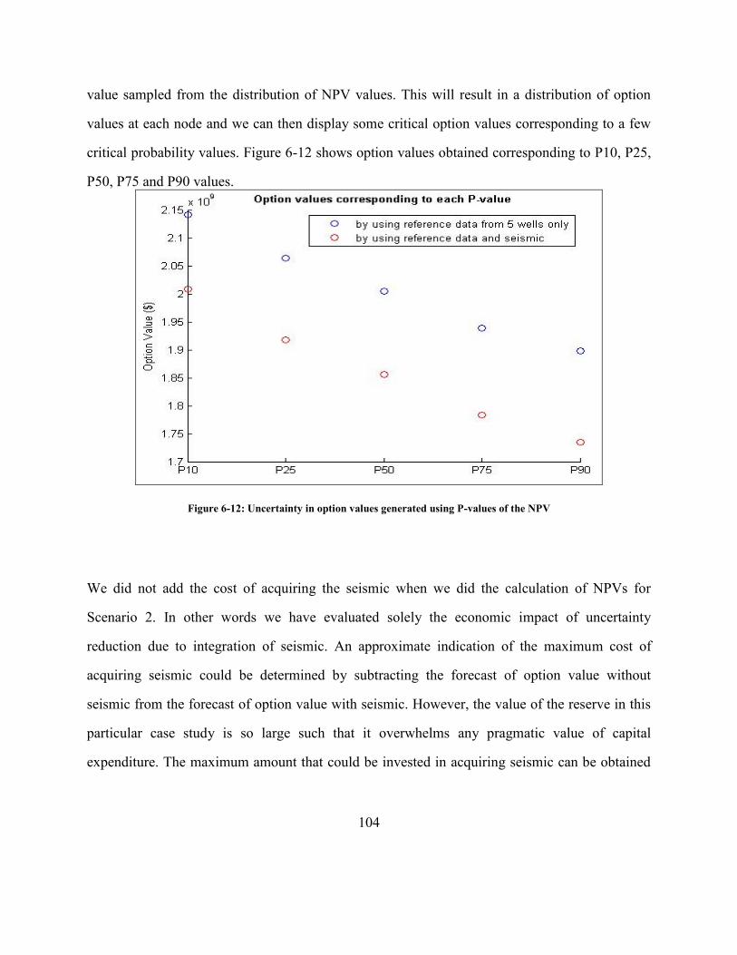
104
value sampled from the distribution of NPV values. This will result in a distribution of option
values at each node and we can then display some critical option values corresponding to a few
critical probability values. Figure 6-12 shows option values obtained corresponding to P10, P25,
P50, P75 and P90 values.
Figure 6-12: Uncertainty in option values generated using P-values of the NPV
We did not add the cost of acquiring the seismic when we did the calculation of NPVs for
Scenario 2. In other words we have evaluated solely the economic impact of uncertainty
reduction due to integration of seismic. An approximate indication of the maximum cost of
acquiring seismic could be determined by subtracting the forecast of option value without
seismic from the forecast of option value with seismic. However, the value of the reserve in this
particular case study is so large such that it overwhelms any pragmatic value of capital
expenditure. The maximum amount that could be invested in acquiring seismic can be obtained

105
from the Figure 6-12 by subtracting the red colored circle values from their respective blue
colored circle values.
The profitability of the field after investing in development costs increases with the increase in
option value. In this case study acquiring seismic over and above existing well data did not
improve the option value (the profitability) or decrease uncertainty of the field. Based on the
results of this specific case study it can be seen that it is hard to improve on value of a large
project. In other words, using seismic to firm up porosity estimates does not seem to work in
large fields.
106
Chapter 7: Uncertainty Analysis by Model Selection and Economic
Evaluation Using a Binomial Lattice
INTRODUCTION
In general, geological uncertainty analysis implies multiple spatial realizations of geological
attributes using stochastic spatial simulation. These multiple realizations represent the spatial
variations of the reservoir attributes. Processing these realizations through a transfer function
model yields the uncertainty in flow response of the reservoir.
In integrated risk assessment studies, the uncertainty from one aspect of the study is carried to
another aspect, and gets aggregated. A model selection framework does the work of refining an
initial suite of reservoir models to a final set of reservoir models that depict production
characteristics close to the observed field history. In this chapter we present a model selection
algorithm which attempts to group reservoir models based on the common connectivity
characteristics exhibited by them and then retrieves the group exhibiting characteristics that are
closest to the observed response for a reservoir. The model selection technique is thus an
efficient way to reduce number of realizations and save computational time for doing uncertainty
analysis, and yet be optimally constrained to the available data.
MODEL SELECTION ALGORITHM
We use the distance-metric based approach proposed by Bhowmik et al. (Bhowmik et al. 2010)
for reservoir model selection. The method uses a proxy function to discriminate between models
on the basis of their connectivity characteristics.
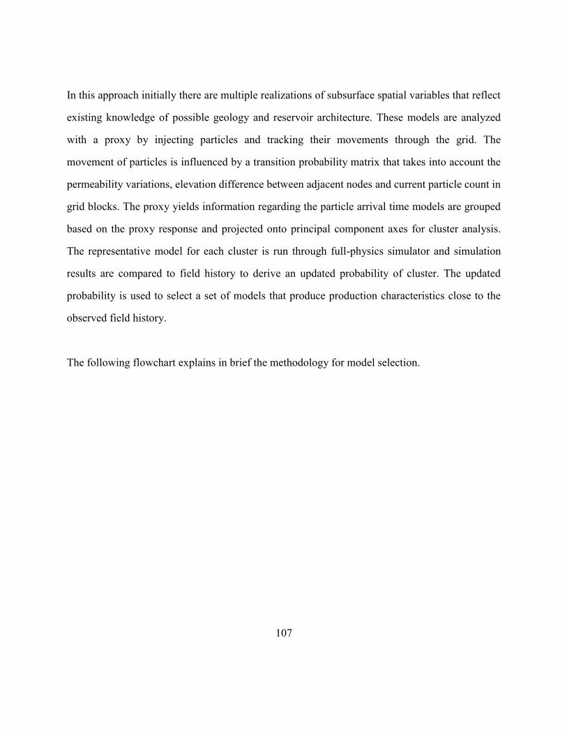
107
In this approach initially there are multiple realizations of subsurface spatial variables that reflect
existing knowledge of possible geology and reservoir architecture. These models are analyzed
with a proxy by injecting particles and tracking their movements through the grid. The
movement of particles is influenced by a transition probability matrix that takes into account the
permeability variations, elevation difference between adjacent nodes and current particle count in
grid blocks. The proxy yields information regarding the particle arrival time models are grouped
based on the proxy response and projected onto principal component axes for cluster analysis.
The representative model for each cluster is run through full-physics simulator and simulation
results are compared to field history to derive an updated probability of cluster. The updated
probability is used to select a set of models that produce production characteristics close to the
observed field history.
The following flowchart explains in brief the methodology for model selection.
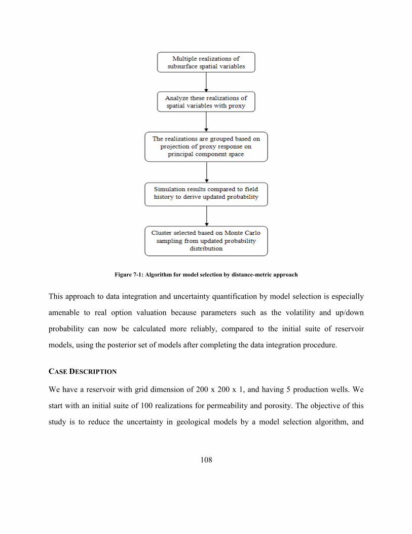
108
Figure 7-1: Algorithm for model selection by distance-metric approach
This approach to data integration and uncertainty quantification by model selection is especially
amenable to real option valuation because parameters such as the volatility and up/down
probability can now be calculated more reliably, compared to the initial suite of reservoir
models, using the posterior set of models after completing the data integration procedure.
CASE DESCRIPTION
We have a reservoir with grid dimension of 200 x 200 x 1, and having 5 production wells. We
start with an initial suite of 100 realizations for permeability and porosity. The objective of this
study is to reduce the uncertainty in geological models by a model selection algorithm, and
109
subsequently apply the binomial lattice option valuation to compare the economics before and
after data integration.
We want to reduce the uncertainty in the geological models, but we also want that reduction in
uncertainty to be robust. In this case, we assume that well test data is available for two different
wells. By assuming that the well test data are non-interfering, we implement the model selection
algorithm two times, each time using the well test data for one well to obtain two sets of geologic
models. The final set of geologic models is selected by retaining the models that are common
between the two sets. This procedure leaves just 4 sets of geologic models as opposed to a suite
of 100 models when we started. Additional models that exhibit characteristics similar to the final
set of models can be generated by retrieving spatial statistics (variogram or multiple point
statistics) that are common to the models and common conditioning data values from the models.
These models will share the production characteristics that are reflected in the final set of four
models.
Finally, future hydrocarbon production rates are determined from the final set of geologic models
and the reservoir‟s economic performance is assessed using the forecast of hydrocarbon
production rates.
STATIC RESERVOIR MODELING
The hard data of porosity and permeability from the 5 production wells are sampled from the
reference. Porosity and permeability maps are developed using SISIM program, which is a
variogram-based geostatistical simulation technique. As inputto the SISIM simulation program,
we use 5 hard data sampled from the reference data. The variogram model is developed using

110
105 sampled data from the reference, which includes the data from 5 wells locations as well,
corresponding to the median threshold. The hard data as well as the semivariogram models for
porosity and permeability, respectively, are given in Table 7-1:
Table 7-1: Hard data of porosity and permeability from 5 reference wells
Shown in Figure 7-2 is an isotropic model fit (black line) fitted on the experimental variograms
(red points) of porosity in various directions:
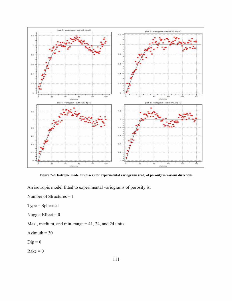
111
Figure 7-2: Isotropic model fit (black) for experimental variograms (red) of porosity in various directions
An isotropic model fitted to experimental variograms of porosity is:
Number of Structures = 1
Type = Spherical
Nugget Effect = 0
Max., medium, and min. range = 41, 24, and 24 units
Azimuth = 30
Dip = 0
Rake = 0

112
Similarly, shown in Figure 7-3 is an isotropic model fit (black line) fitted on the experimental
variograms (red points) of permeability in various directions:
Figure 7-3: Isotropic model fit (black) for experimental variograms (red) of permeability in various directions
An isotropic model fitted to experimental variograms of permeability is:
Number of Structures = 1
Type = Spherical
Nugget Effect = 0
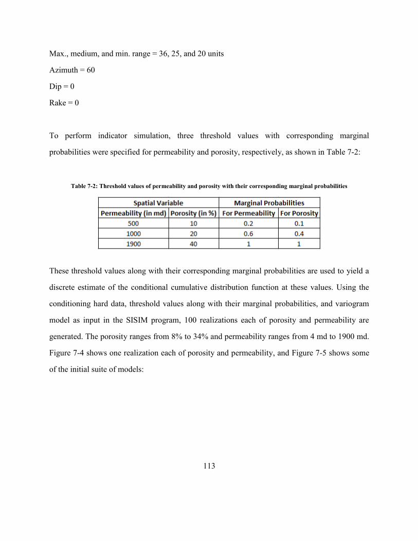
113
Max., medium, and min. range = 36, 25, and 20 units
Azimuth = 60
Dip = 0
Rake = 0
To perform indicator simulation, three threshold values with corresponding marginal
probabilities were specified for permeability and porosity, respectively, as shown in Table 7-2:
Table 7-2: Threshold values of permeability and porosity with their corresponding marginal probabilities
These threshold values along with their corresponding marginal probabilities are used to yield a
discrete estimate of the conditional cumulative distribution function at these values. Using the
conditioning hard data, threshold values along with their marginal probabilities, and variogram
model as input in the SISIM program, 100 realizations each of porosity and permeability are
generated. The porosity ranges from 8% to 34% and permeability ranges from 4 md to 1900 md.
Figure 7-4 shows one realization each of porosity and permeability, and Figure 7-5 shows some
of the initial suite of models:
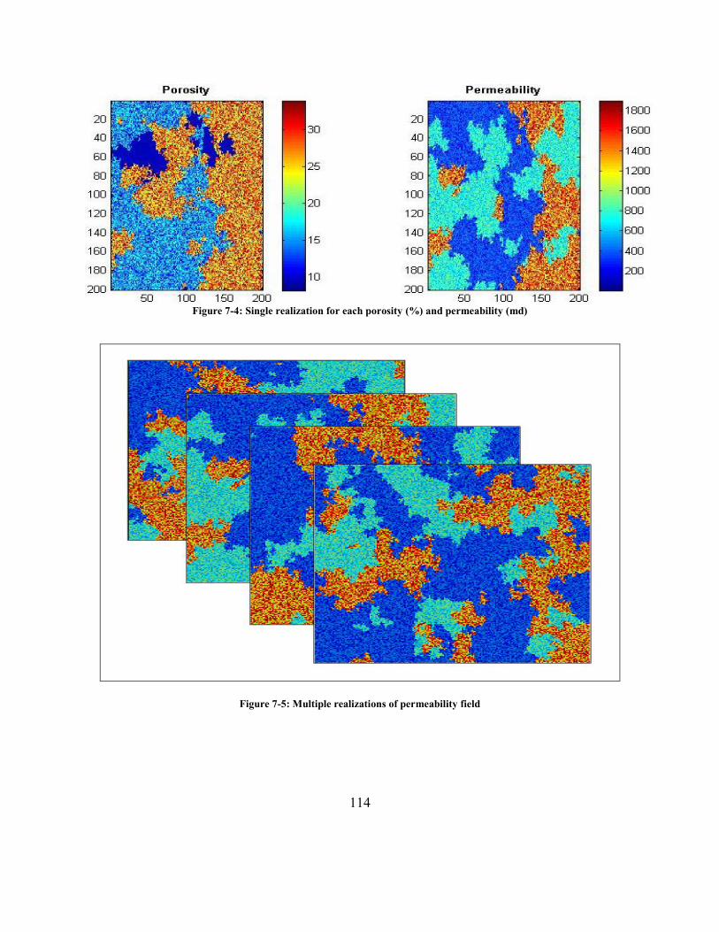
114
Figure 7-4: Single realization for each porosity (%) and permeability (md)
Figure 7-5: Multiple realizations of permeability field
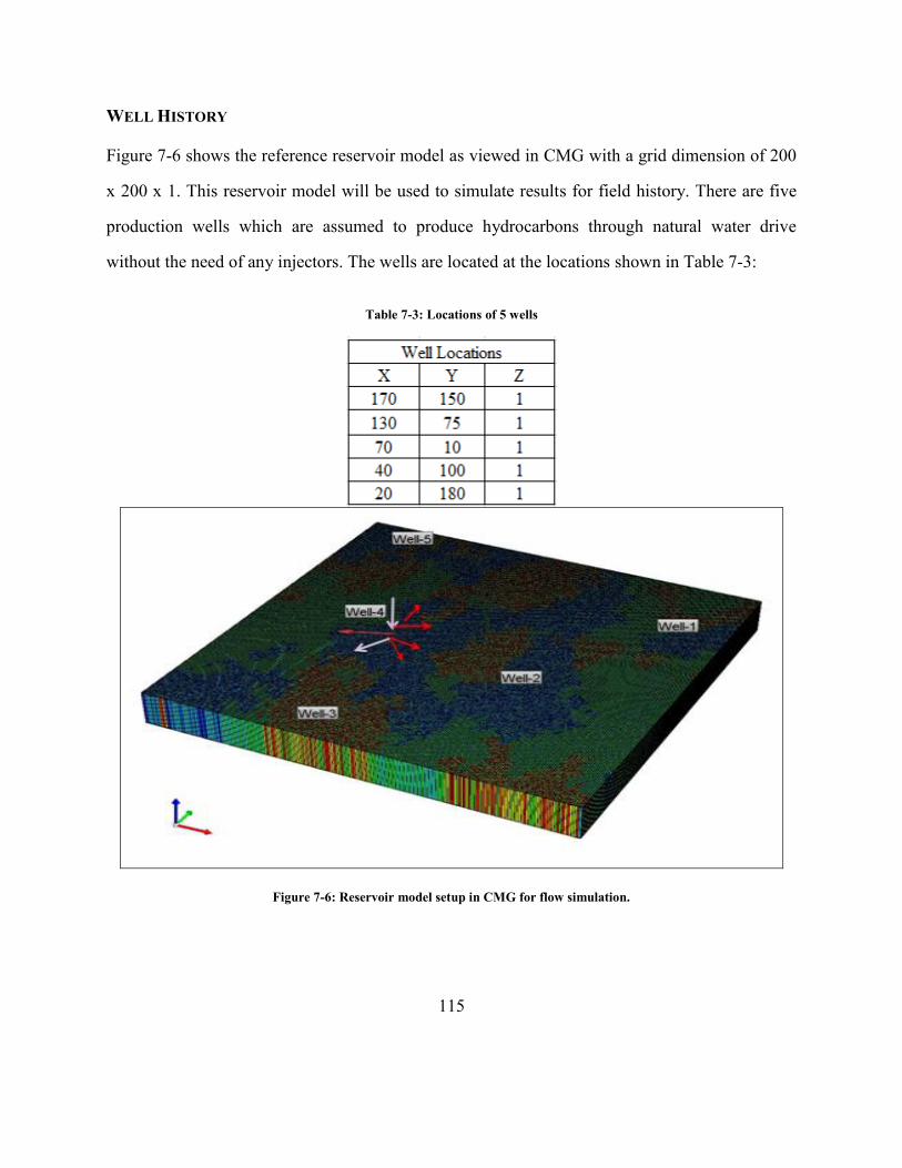
115
WELL HISTORY
Figure 7-6 shows the reference reservoir model as viewed in CMG with a grid dimension of 200
x 200 x 1. This reservoir model will be used to simulate results for field history. There are five
production wells which are assumed to produce hydrocarbons through natural water drive
without the need of any injectors. The wells are located at the locations shown in Table 7-3:
Table 7-3: Locations of 5 wells
Figure 7-6: Reservoir model setup in CMG for flow simulation.
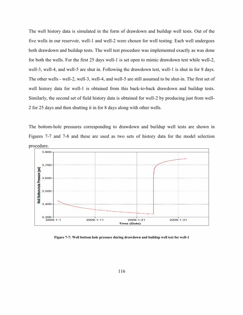
116
The well history data is simulated in the form of drawdown and buildup well tests. Out of the
five wells in our reservoir, well-1 and well-2 were chosen for well testing. Each well undergoes
both drawdown and buildup tests. The well test procedure was implemented exactly as was done
for both the wells. For the first 25 days well-1 is set open to mimic drawdown test while well-2,
well-3, well-4, and well-5 are shut in. Following the drawdown test, well-1 is shut in for 8 days.
The other wells - well-2, well-3, well-4, and well-5 are still assumed to be shut-in. The first set of
well history data for well-1 is obtained from this back-to-back drawdown and buildup tests.
Similarly, the second set of field history data is obtained for well-2 by producing just from well-
2 for 25 days and then shutting it in for 8 days along with other wells.
The bottom-hole pressures corresponding to drawdown and buildup well tests are shown in
Figures 7-7 and 7-8 and these are used as two sets of history data for the model selection
procedure.
Figure 7-7: Well bottom hole pressure during drawdown and buildup well test for well-1

117
Figure 7-8: Well bottom hole pressure during drawdown and buildup well test for well-2
A particle tracking algorithm that mimics the propagation of the pressure wave during a well test
was used as the proxy to assess the flow response of the models in the prior set. Details of this
proxy can be found in Bhowmik et al. (Bhowmik et al. 2010).
FINAL SET OF MODELS BY MODEL SELECTION ALGORITHM
After applying the model selection algorithm on the initial suite of models we obtain 5 models
for each set of field history data. Out of these 10 total models in the final set, 4 are common.
These four models exhibit similar well test characteristics for well – 1 and 2 as observed in the
reference.
The reduction of the prior set of 100 models to just 4 models is quite significant. These selected
models will not only carry the same statistics from the suite of prior models, but they will also
have the same flow characteristic as the prior models. Figure 7-9 shows the uncertainty in future
hydrocarbon production rates for 20 years both prior to and after model selection. The

118
uncertainty in production rates represented by 100 realizations (in blue legend) before model
selection reduces to in the spread indicated by the red legend.
Figure 7-9: Uncertainty in oil flow rates from the reservoir before and after model selection
The oil rate predicted by the final set of models is closer but not exactly the same as the
reference. This is because the well test response recorded only at wells 1 and 2 were used for the
model selection process and they are insufficient to capture the connectivity characteristics of the
entire field. Consequently, the oil rate characteristics are not well represented by the models.
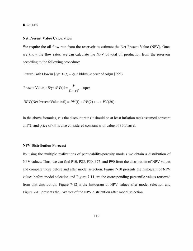
119
RESULTS
Net Present Value Calculation
We require the oil flow rate from the reservoir to estimate the Net Present Value (NPV). Once
we know the flow rates, we can calculate the NPV of total oil production from the reservoir
according to the following procedure:
FutureCash Flow in $/yr : ( ) (in bbl/yr) priceof oil(in $/bbl)
Present Valuein $/yr : ( ) opex(1 )
(Net Present Valuein $) (1) (2) ... (20)
t
F t q
FPV t
r
NPV PV PV PV
In the above formulas, r is the discount rate (it should be at least inflation rate) assumed constant
at 5%, and price of oil is also considered constant with value of $70/barrel.
NPV Distribution Forecast
By using the multiple realizations of permeability-porosity models we obtain a distribution of
NPV values. Thus, we can find P10, P25, P50, P75, and P90 from the distribution of NPV values
and compare those before and after model selection. Figure 7-10 presents the histogram of NPV
values before model selection and Figure 7-11 are the corresponding percentile values retrieved
from that distribution. Figure 7-12 is the histogram of NPV values after model selection and
Figure 7-13 presents the P-values of the NPV distribution after model selection.

120
The uncertainty represented by the NPV distribution, before and after model selection, is because
of the uncertainty in geologic models. The forecast of flow rate prediction using models before
model selection is quite wide and this is confirmed by the greater spread in NPV values (Figure
7-10). The forecast of flow rate prediction after model selection is narrower than flow rate
prediction from initial suite of models and this is also confirmed by the tighter range of NPV
distribution (Figure 7-12) after model selection compared to the the greater spread in NPV values
before model selection .
Before Model Selection:
Figure 7-10: NPV distribution before model selection
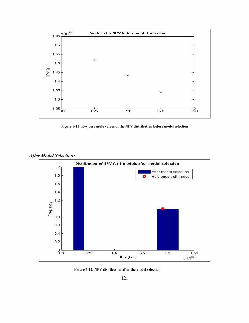
121
Figure 7-11: Key percentile values of the NPV distribution before model selection
After Model Selection:
Figure 7-12: NPV distribution after the model selection

122
Figure 7-13: Key percentiles of the NPV distribution after the model selection
We want to incorporate the uncertainty represented by the NPV before and after model selection
into the Binomial Lattice Option Valuation (BLOV). BLOV takes a single value of the NPV as
input in the starting node of the underlying lattice. To incorporate the uncertainty from the NPV
distribution, we take the weighted average of the P-values of the NPV distribution to come up
with the NPV value at the starting node of the BLOV. This method of computing the single value
of NPV, which will be used as input in the underlying lattice, incorporates the uncertainty before
and after model selection.
Project Volatility
The future cash flows discussed under the NPV section will be used to compute the project
volatility through the method explained in Chapter 2 and implemented in previous chapters.

123
This project volatility is one of the most critical parameter which is used as input in the real
options model. We calculated the project volatility as following:
( ) ( ) ( )PV t F t DV t
1
0
h
ln
( )
where,
Present value at i year
std( ) Standard deviation
Project Volatility
n
i
i
n
i
i
t
i
PV
G
PV
std G
PV
Figure 7-14 shows that the calculated time-varying project volatility decreases with time. The
reason of decrease in project volatility with time is due to the fact that with time there is increase
in prior data of the reservoir‟s economic performance (in terms of DCF). The project volatility
for reference truth is developed using the 2nd
realization of reference truth available. In total there
were only two realizations of reference truth available, and the model comparison is done
everywhere with the first realization of reference truth model.

124
Figure 7-14: Variation of project volatility with time for models before and after selection, and reference truth
For BLOV, the volatility is assumed to be constant throughout the lattice construction. In our
case we took the first value of volatility predicted at the second year for all the scenarios. This is
a conservative estimate for the project volatility but one that simplifies the lattice generation for
ROV calculations.
Option Valuation by BLOV
Figure 7-15 shows the lattice of the underlying asset for reference truth model while Figure 7-16
shows the option valuation lattice. Similarly, Figures 7-17 and 7-19 show the lattice of the
underlying asset before and after model selection, respectively, while Figures 7-18 and 7-20
show their corresponding option valuation lattices, respectively.
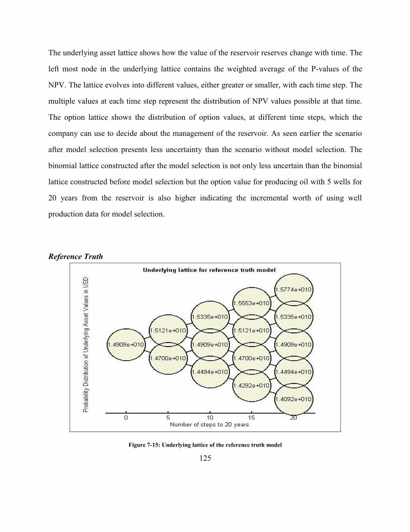
125
The underlying asset lattice shows how the value of the reservoir reserves change with time. The
left most node in the underlying lattice contains the weighted average of the P-values of the
NPV. The lattice evolves into different values, either greater or smaller, with each time step. The
multiple values at each time step represent the distribution of NPV values possible at that time.
The option lattice shows the distribution of option values, at different time steps, which the
company can use to decide about the management of the reservoir. As seen earlier the scenario
after model selection presents less uncertainty than the scenario without model selection. The
binomial lattice constructed after the model selection is not only less uncertain than the binomial
lattice constructed before model selection but the option value for producing oil with 5 wells for
20 years from the reservoir is also higher indicating the incremental worth of using well
production data for model selection.
Reference Truth
Figure 7-15: Underlying lattice of the reference truth model
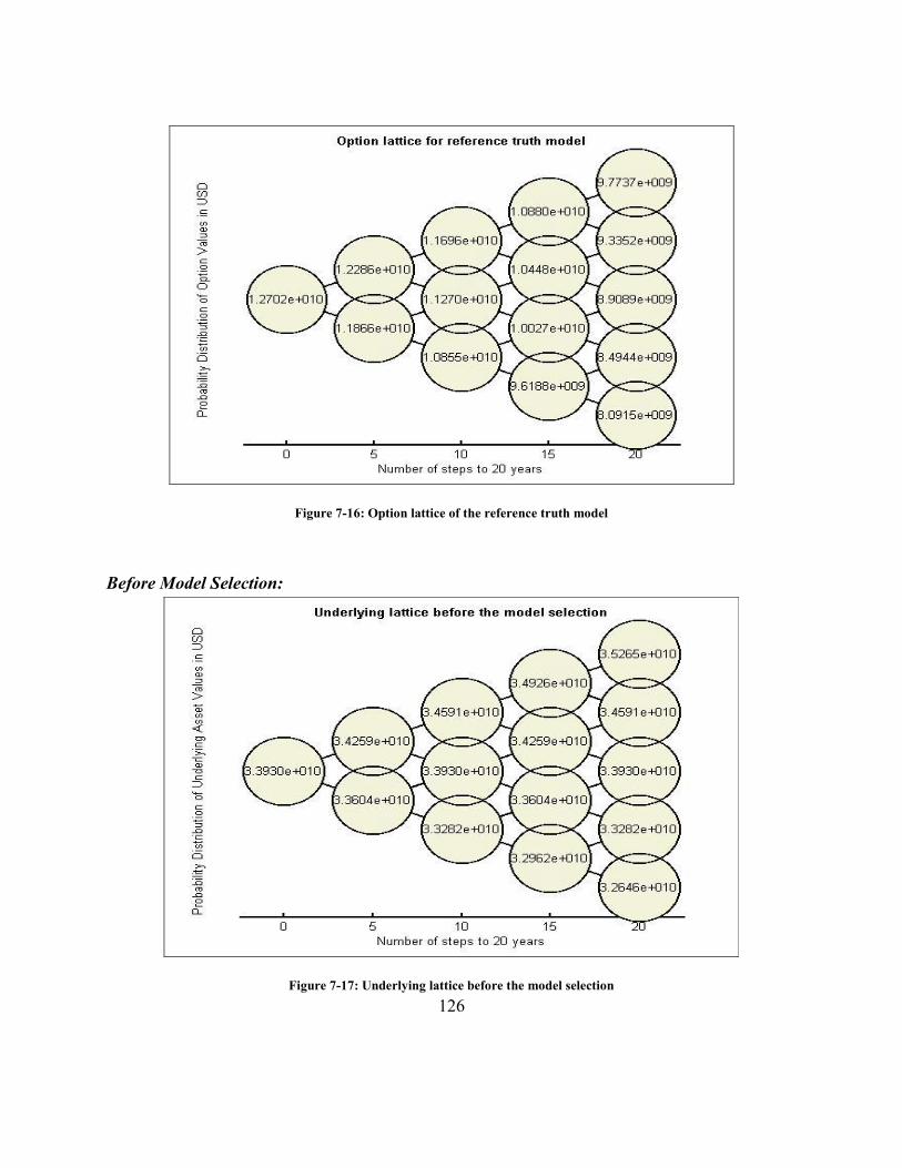
126
Figure 7-16: Option lattice of the reference truth model
Before Model Selection:
Figure 7-17: Underlying lattice before the model selection

127
Figure 7-18: Option lattice before the model selection
After Model Selection:
Figure 7-19: Underlying lattice after the model selection
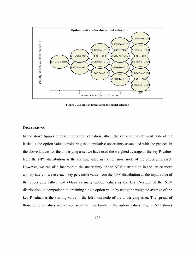
128
Figure 7-20: Option lattice after the model selection
DISCUSSIONS
In the above figures representing option valuation lattice, the value in the left most node of the
lattice is the option value considering the cumulative uncertainty associated with the project. In
the above lattices for the underlying asset we have used the weighted average of the key P-values
from the NPV distribution as the starting value in the left most node of the underlying asset.
However, we can also incorporate the uncertainty of the NPV distribution in the lattice more
appropriately if we use each key percentile value from the NPV distribution as the input value of
the underlying lattice and obtain as many option values as the key P-values of the NPV
distribution, in comparison to obtaining single option value by using the weighted average of the
key P-values as the starting value in the left most node of the underlying asset. The spread of
those options values would represent the uncertainty in the option values. Figure 7-21 shows
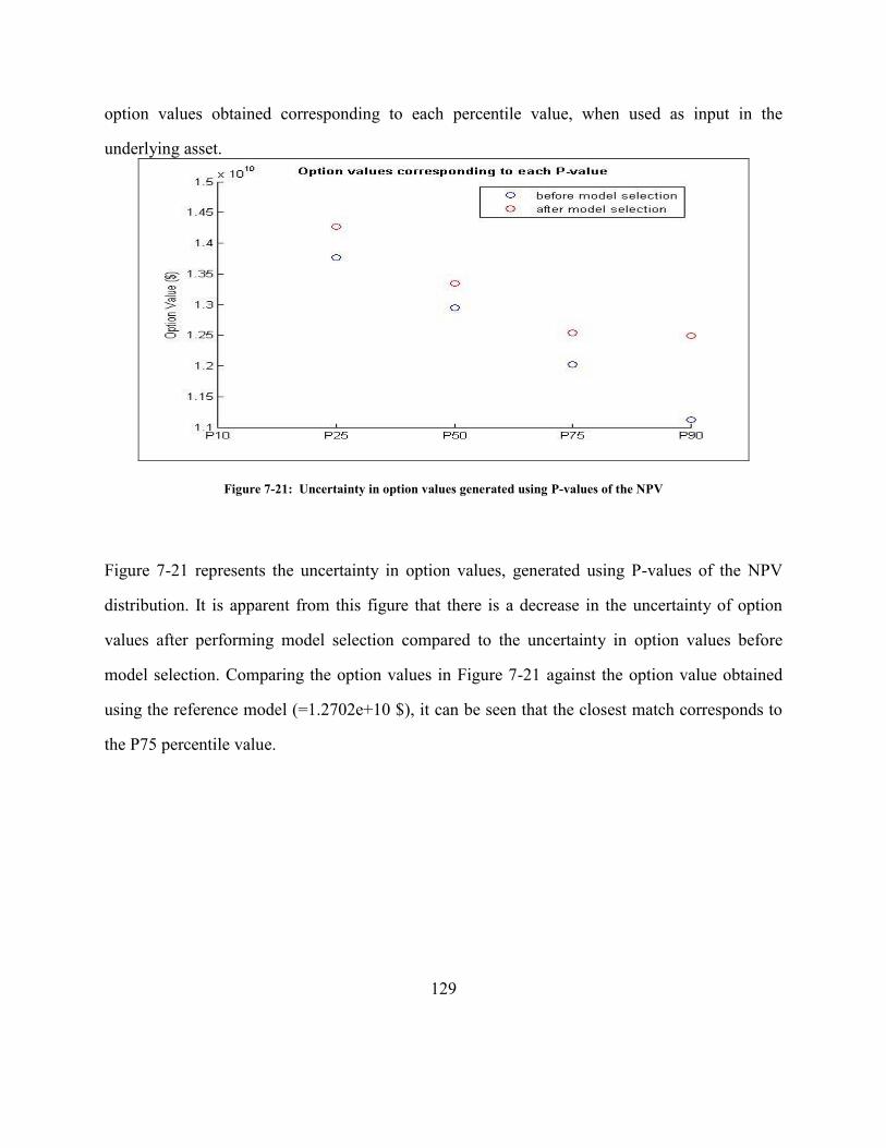
129
option values obtained corresponding to each percentile value, when used as input in the
underlying asset.
Figure 7-21: Uncertainty in option values generated using P-values of the NPV
Figure 7-21 represents the uncertainty in option values, generated using P-values of the NPV
distribution. It is apparent from this figure that there is a decrease in the uncertainty of option
values after performing model selection compared to the uncertainty in option values before
model selection. Comparing the option values in Figure 7-21 against the option value obtained
using the reference model (=1.2702e+10 $), it can be seen that the closest match corresponds to
the P75 percentile value.
130
Chapter 8: Summary, Conclusions, and Future Recommendations
SUMMARY
Project evaluation under uncertainty is a key aspect of reservoir engineering and management
that has assumed a critical role in recent times due to the depletion of easy to produce
hydrocarbon resources and the increasing hostile operating environments faced by oil and gas
operators. In light of the multi-domain uncertainties that confront major projects – flexibility in
making development decisions is essential. This necessitates the use of ROV for strategic
planning and decision-making in upstream petroleum industry projects.
This thesis addressed the following research questions:
A strategy to assess the economic worth of incremental data by progressively updating
reservoir models. The incremental source of data was either an exploratory well or a
seismic. Results suggested that neither of the two information brought significant
improvement in resolving the uncertainty within the ROV framework.
Comparison of reservoir performance based on varying levels of detail in geological
model and flow model. ROV analysis is used to address the issue of optimal
representation of geology in reservoir models and the role of complex flow models in
context of long term uncertainty analysis and risk assessment. Results seem to indicate
that complexity in models might not always translate to improved accuracies in economic
forecasts. Also, all the economic forecast results suggest that ROV could highlight hidden
value of reservoir which NPV fails to uncover.
Extension of ROV framework using Binomial Lattice, which is easy to use, easy to
understand, and more accurate, particularly for longer periods. The BLOV framework is

131
applied to analyze the economic prospects of an undeveloped, but discovered field.
Assessing option values on temporal scale presents the flexibility to make time dependent
development decisions.
A strategy to reduce the cost of investment for performing well test by employing the use
of appropriate stochastic reservoir modeling technique and the reference data. The results
suggest that SISIM permeability maps translate into less uncertainty in economic
valuation than the well test permeability. This is based on the fact that SISIM tries to
maintain the continuity in permeability structure of the reservoir as displayed by the
SISIM map.
A strategy to save computational time for doing uncertainty analysis, in context of
reservoir performance and risk assessment, by employing the use of model selection
algorithm. It results in reduction in prior set of 100 models to just 4 models that exhibit
production behavior similar to the observed history. It helps in making the uncertainty
quantification feasible and simpler.
CONCLUSIONS
The following conclusions can presented based on the work in this thesis:
ROV uncovers hidden economic potential of hydrocarbon prospects that conventional
DCF analysis might not identify.
Acquiring extra information might not always be valuable in terms of reducing
uncertainty and better economic forecast.
Complexity in reservoir and flow models might not always translate to improved
accuracies in economic forecasts.
132
BLOV is easier to easy to use and easy to understand compared to the continuous ROV
using Black-Scholes model.
The model selection algorithm is an efficient and simpler way to do uncertainty
quantification by significantly reducing the number of reservoir models from prior suite
of reservoir models.
RECOMMENDATIONS FOR FUTURE WORK
On the basis of work done in this thesis, and to explore the full potential of ROV in upstream
petroleum industry projects, following can be recommended for future studies:
Real Data Modeling: The stochastic reservoir models developed in this thesis for
uncertainty analysis were not based on real field data or historical data of analogues
projects. It would be interesting to see the results of uncertainty modeling and ROV
based on reservoir models developed using real field data.
Explore Model Complexity for Short Term Projects: The forecast of hydrocarbon
production rates and economic valuation of the projects done in this thesis are for long
term projects in range of several years. Performing ROV for short term projects and the
effect of complexity in reservoir models in final economic forecast may be useful in
determining the how the ROV is affected by complexity in reservoir models for short
term projects.
Extend Project Volatility Model: Extension of the volatility models which can include
negative present worth or market value of a project.
Explore Facilities Cost Modeling: This thesis assumes an approximate cost for
development of facilities. To investigate how the facilities cost influences ROV, it is

133
important to use the facilities cost models to calculate facilities cost based on the planned
production capacity.
Explore Market Uncertainties: This thesis assumes constant market parameters like
interest rate, cost of operational expenses etc. To investigate the effect of market
uncertainties, it is important to vary these parameters based on market conditions.

134
Appendix A: Simulation Data Files for CMG-IMEX
This appendix presents CMG-IMEX simulation data files for various cases presented in this
thesis.
A.1 RESERVOIR MODEL: 50 X 50 X 1GRID DIMENSION, 5 PRODUCTION WELLS (CHAPTER 3)
RESULTS SIMULATOR IMEX 200900
INTERRUPT RESTART-STOP
INUNIT FIELD
WSRF WELL 1
WSRF GRID TIME
WSRF SECTOR TIME
OUTSRF WELL LAYER NONE
OUTSRF RES ALL
OUTSRF GRID BPP OILPOT PRES SO SSPRES SW WINFLUX
WPRN GRID 0
OUTPRN GRID NONE
OUTPRN RES NONE
**$ Distance units: ft
RESULTS XOFFSET 0.0000
RESULTS YOFFSET 0.0000
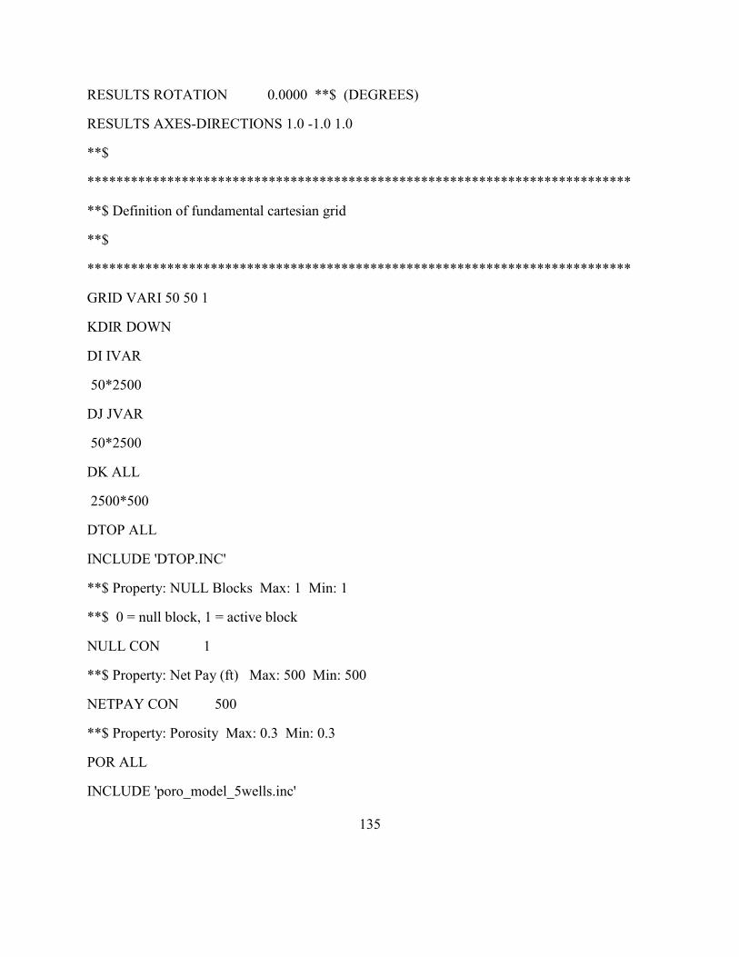
135
RESULTS ROTATION 0.0000 **$ (DEGREES)
RESULTS AXES-DIRECTIONS 1.0 -1.0 1.0
**$
***************************************************************************
**$ Definition of fundamental cartesian grid
**$
***************************************************************************
GRID VARI 50 50 1
KDIR DOWN
DI IVAR
50*2500
DJ JVAR
50*2500
DK ALL
2500*500
DTOP ALL
INCLUDE 'DTOP.INC'
**$ Property: NULL Blocks Max: 1 Min: 1
**$ 0 = null block, 1 = active block
NULL CON 1
**$ Property: Net Pay (ft) Max: 500 Min: 500
NETPAY CON 500
**$ Property: Porosity Max: 0.3 Min: 0.3
POR ALL
INCLUDE 'poro_model_5wells.inc'
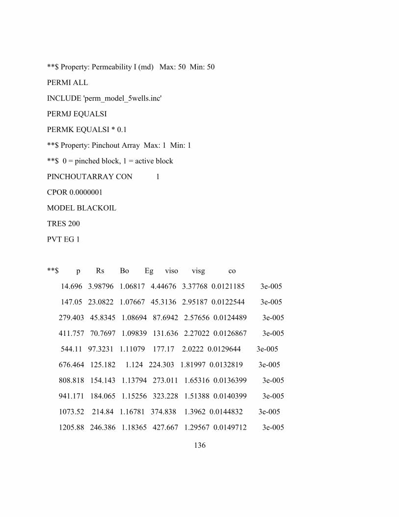
136
**$ Property: Permeability I (md) Max: 50 Min: 50
PERMI ALL
INCLUDE 'perm_model_5wells.inc'
PERMJ EQUALSI
PERMK EQUALSI * 0.1
**$ Property: Pinchout Array Max: 1 Min: 1
**$ 0 = pinched block, 1 = active block
PINCHOUTARRAY CON 1
CPOR 0.0000001
MODEL BLACKOIL
TRES 200
PVT EG 1
**$ p Rs Bo Eg viso visg co
14.696 3.98796 1.06817 4.44676 3.37768 0.0121185 3e-005
147.05 23.0822 1.07667 45.3136 2.95187 0.0122544 3e-005
279.403 45.8345 1.08694 87.6942 2.57656 0.0124489 3e-005
411.757 70.7697 1.09839 131.636 2.27022 0.0126867 3e-005
544.11 97.3231 1.11079 177.17 2.0222 0.0129644 3e-005
676.464 125.182 1.124 224.303 1.81997 0.0132819 3e-005
808.818 154.143 1.13794 273.011 1.65316 0.0136399 3e-005
941.171 184.065 1.15256 323.228 1.51388 0.0140399 3e-005
1073.52 214.84 1.16781 374.838 1.3962 0.0144832 3e-005
1205.88 246.386 1.18365 427.667 1.29567 0.0149712 3e-005
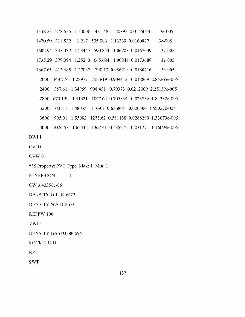
137
1338.23 278.635 1.20006 481.48 1.20892 0.0155044 3e-005
1470.59 311.532 1.217 535.986 1.13339 0.0160827 3e-005
1602.94 345.032 1.23447 590.844 1.06708 0.0167049 3e-005
1735.29 379.094 1.25243 645.684 1.00844 0.0173689 3e-005
1867.65 413.685 1.27087 700.13 0.956218 0.0180716 3e-005
2000 448.776 1.28977 753.819 0.909442 0.018809 2.85265e-005
2400 557.61 1.34959 908.451 0.79373 0.0212009 2.25139e-005
2800 670.199 1.41321 1047.64 0.705834 0.023736 1.84332e-005
3200 786.11 1.48035 1169.7 0.636804 0.026304 1.55027e-005
3600 905.01 1.55082 1275.62 0.581138 0.0288299 1.33079e-005
4000 1026.63 1.62442 1367.41 0.535275 0.031271 1.16098e-005
BWI 1
CVO 0
CVW 0
**$ Property: PVT Type Max: 1 Min: 1
PTYPE CON 1
CW 3.43356e-06
DENSITY OIL 54.6422
DENSITY WATER 60
REFPW 100
VWI 1
DENSITY GAS 0.0686695
ROCKFLUID
RPT 1
SWT
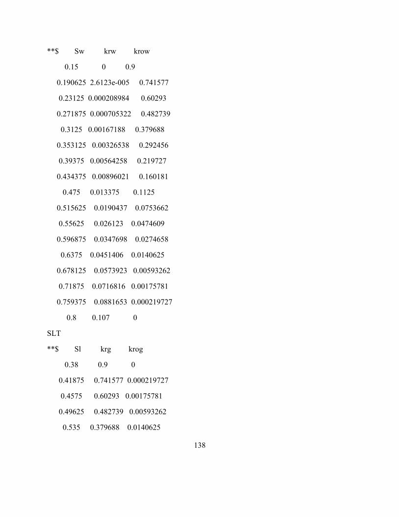
138
**$ Sw krw krow
0.15 0 0.9
0.190625 2.6123e-005 0.741577
0.23125 0.000208984 0.60293
0.271875 0.000705322 0.482739
0.3125 0.00167188 0.379688
0.353125 0.00326538 0.292456
0.39375 0.00564258 0.219727
0.434375 0.00896021 0.160181
0.475 0.013375 0.1125
0.515625 0.0190437 0.0753662
0.55625 0.026123 0.0474609
0.596875 0.0347698 0.0274658
0.6375 0.0451406 0.0140625
0.678125 0.0573923 0.00593262
0.71875 0.0716816 0.00175781
0.759375 0.0881653 0.000219727
0.8 0.107 0
SLT
**$ Sl krg krog
0.38 0.9 0
0.41875 0.741577 0.000219727
0.4575 0.60293 0.00175781
0.49625 0.482739 0.00593262
0.535 0.379688 0.0140625

139
0.57375 0.292456 0.0274658
0.6125 0.219727 0.0474609
0.65125 0.160181 0.0753662
0.69 0.1125 0.1125
0.72875 0.0753662 0.160181
0.7675 0.0474609 0.219727
0.80625 0.0274658 0.292456
0.845 0.0140625 0.379688
0.88375 0.00593262 0.482739
0.9225 0.00175781 0.60293
0.96125 0.000219727 0.741577
1 0 0.9
INITIAL
VERTICAL DEPTH_AVE WATER_OIL EQUIL
REFDEPTH 1000
REFPRES 4000
DWOC 1500
**$ Property: Bubble Point Pressure (psi) Max: 0 Min: 0
PB CON 0
NUMERICAL
RUN
DATE 2009 1 1
**$
WELL 'Well-1'
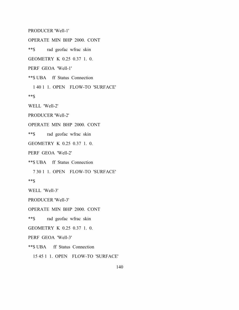
140
PRODUCER 'Well-1'
OPERATE MIN BHP 2000. CONT
**$ rad geofac wfrac skin
GEOMETRY K 0.25 0.37 1. 0.
PERF GEOA 'Well-1'
**$ UBA ff Status Connection
1 40 1 1. OPEN FLOW-TO 'SURFACE'
**$
WELL 'Well-2'
PRODUCER 'Well-2'
OPERATE MIN BHP 2000. CONT
**$ rad geofac wfrac skin
GEOMETRY K 0.25 0.37 1. 0.
PERF GEOA 'Well-2'
**$ UBA ff Status Connection
7 30 1 1. OPEN FLOW-TO 'SURFACE'
**$
WELL 'Well-3'
PRODUCER 'Well-3'
OPERATE MIN BHP 2000. CONT
**$ rad geofac wfrac skin
GEOMETRY K 0.25 0.37 1. 0.
PERF GEOA 'Well-3'
**$ UBA ff Status Connection
15 45 1 1. OPEN FLOW-TO 'SURFACE'
141
**$
WELL 'Well-4'
PRODUCER 'Well-4'
OPERATE MIN BHP 2000. CONT
**$ rad geofac wfrac skin
GEOMETRY K 0.25 0.37 1. 0.
PERF GEOA 'Well-4'
**$ UBA ff Status Connection
23 10 1 1. OPEN FLOW-TO 'SURFACE'
**$
WELL 'Well-5'
PRODUCER 'Well-5'
OPERATE MIN BHP 2000. CONT
**$ rad geofac wfrac skin
GEOMETRY K 0.25 0.37 1. 0.
PERF GEOA 'Well-5'
**$ UBA ff Status Connection
30 43 1 1. OPEN FLOW-TO 'SURFACE'
DATE 2010 1 1.00000
DATE 2011 1 1.00000
DATE 2012 1 1.00000
DATE 2013 1 1.00000
DATE 2014 1 1.00000
DATE 2015 1 1.00000
DATE 2016 1 1.00000
142
DATE 2017 1 1.00000
DATE 2018 1 1.00000
DATE 2019 1 1.00000
DATE 2020 1 1.00000
DATE 2021 1 1.00000
DATE 2022 1 1.00000
DATE 2023 1 1.00000
DATE 2024 1 1.00000
DATE 2025 1 1.00000
DATE 2026 1 1.00000
DATE 2027 1 1.00000
DATE 2028 1 1.00000
DATE 2029 1 1.00000
STOP
A.2 RESERVOIR MODEL: 200 X 200 X 1GRID DIMENSION, 5 PRODUCTION WELLS (CHAPTER
4)
RESULTS SIMULATOR IMEX 200900
INTERRUPT RESTART-STOP
INUNIT FIELD
WSRF WELL 1

143
WSRF GRID TIME
WSRF SECTOR TIME
OUTSRF WELL LAYER NONE
OUTSRF RES ALL
OUTSRF GRID BPP OILPOT PRES SO SSPRES SW WINFLUX
WPRN GRID 0
OUTPRN GRID NONE
OUTPRN RES NONE
**$ Distance units: ft
RESULTS XOFFSET 0.0000
RESULTS YOFFSET 0.0000
RESULTS ROTATION 0.0000 **$ (DEGREES)
RESULTS AXES-DIRECTIONS 1.0 -1.0 1.0
**$
***************************************************************************
**$ Definition of fundamental cartesian grid
**$
***************************************************************************
GRID VARI 200 200 1
KDIR DOWN
DI IVAR
200*2500
DJ JVAR
200*2500
DK ALL

144
40000*500
DTOP ALL
INCLUDE 'DTOP.INC'
**$ Property: NULL Blocks Max: 1 Min: 1
**$ 0 = null block, 1 = active block
NULL CON 1
**$ Property: Net Pay (ft) Max: 500 Min: 500
NETPAY CON 500
**$ Property: Porosity Max: 0.3 Min: 0.3
POR ALL
INCLUDE 'poro_model_5wells_sisim.inc'
**$ Property: Permeability I (md) Max: 50 Min: 50
PERMI ALL
INCLUDE 'perm_model_5wells_sisim.inc'
PERMJ EQUALSI
PERMK EQUALSI * 0.1
**$ Property: Pinchout Array Max: 1 Min: 1
**$ 0 = pinched block, 1 = active block
PINCHOUTARRAY CON 1
CPOR 0.0000001
MODEL BLACKOIL
TRES 200
PVT EG 1
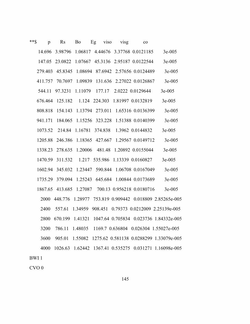
145
**$ p Rs Bo Eg viso visg co
14.696 3.98796 1.06817 4.44676 3.37768 0.0121185 3e-005
147.05 23.0822 1.07667 45.3136 2.95187 0.0122544 3e-005
279.403 45.8345 1.08694 87.6942 2.57656 0.0124489 3e-005
411.757 70.7697 1.09839 131.636 2.27022 0.0126867 3e-005
544.11 97.3231 1.11079 177.17 2.0222 0.0129644 3e-005
676.464 125.182 1.124 224.303 1.81997 0.0132819 3e-005
808.818 154.143 1.13794 273.011 1.65316 0.0136399 3e-005
941.171 184.065 1.15256 323.228 1.51388 0.0140399 3e-005
1073.52 214.84 1.16781 374.838 1.3962 0.0144832 3e-005
1205.88 246.386 1.18365 427.667 1.29567 0.0149712 3e-005
1338.23 278.635 1.20006 481.48 1.20892 0.0155044 3e-005
1470.59 311.532 1.217 535.986 1.13339 0.0160827 3e-005
1602.94 345.032 1.23447 590.844 1.06708 0.0167049 3e-005
1735.29 379.094 1.25243 645.684 1.00844 0.0173689 3e-005
1867.65 413.685 1.27087 700.13 0.956218 0.0180716 3e-005
2000 448.776 1.28977 753.819 0.909442 0.018809 2.85265e-005
2400 557.61 1.34959 908.451 0.79373 0.0212009 2.25139e-005
2800 670.199 1.41321 1047.64 0.705834 0.023736 1.84332e-005
3200 786.11 1.48035 1169.7 0.636804 0.026304 1.55027e-005
3600 905.01 1.55082 1275.62 0.581138 0.0288299 1.33079e-005
4000 1026.63 1.62442 1367.41 0.535275 0.031271 1.16098e-005
BWI 1
CVO 0

146
CVW 0
**$ Property: PVT Type Max: 1 Min: 1
PTYPE CON 1
CW 3.43356e-06
DENSITY OIL 54.6422
DENSITY WATER 60
REFPW 100
VWI 1
DENSITY GAS 0.0686695
ROCKFLUID
RPT 1
SWT
**$ Sw krw krow
0.15 0 0.9
0.190625 2.6123e-005 0.741577
0.23125 0.000208984 0.60293
0.271875 0.000705322 0.482739
0.3125 0.00167188 0.379688
0.353125 0.00326538 0.292456
0.39375 0.00564258 0.219727
0.434375 0.00896021 0.160181
0.475 0.013375 0.1125
0.515625 0.0190437 0.0753662
0.55625 0.026123 0.0474609
0.596875 0.0347698 0.0274658
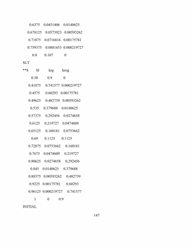
147
0.6375 0.0451406 0.0140625
0.678125 0.0573923 0.00593262
0.71875 0.0716816 0.00175781
0.759375 0.0881653 0.000219727
0.8 0.107 0
SLT
**$ Sl krg krog
0.38 0.9 0
0.41875 0.741577 0.000219727
0.4575 0.60293 0.00175781
0.49625 0.482739 0.00593262
0.535 0.379688 0.0140625
0.57375 0.292456 0.0274658
0.6125 0.219727 0.0474609
0.65125 0.160181 0.0753662
0.69 0.1125 0.1125
0.72875 0.0753662 0.160181
0.7675 0.0474609 0.219727
0.80625 0.0274658 0.292456
0.845 0.0140625 0.379688
0.88375 0.00593262 0.482739
0.9225 0.00175781 0.60293
0.96125 0.000219727 0.741577
1 0 0.9
INITIAL

148
VERTICAL DEPTH_AVE WATER_OIL EQUIL
REFDEPTH 1000
REFPRES 4000
DWOC 1500
**$ Property: Bubble Point Pressure (psi) Max: 0 Min: 0
PB CON 0
NUMERICAL
RUN
DATE 2009 1 1
**$
WELL 'Well-1'
PRODUCER 'Well-1'
OPERATE MIN BHP 2000. CONT
**$ rad geofac wfrac skin
GEOMETRY K 0.25 0.37 1. 0.
PERF GEOA 'Well-1'
**$ UBA ff Status Connection
170 50 1 1. OPEN FLOW-TO 'SURFACE'
**$
WELL 'Well-2'
PRODUCER 'Well-2'
OPERATE MIN BHP 2000. CONT
**$ rad geofac wfrac skin
GEOMETRY K 0.25 0.37 1. 0.
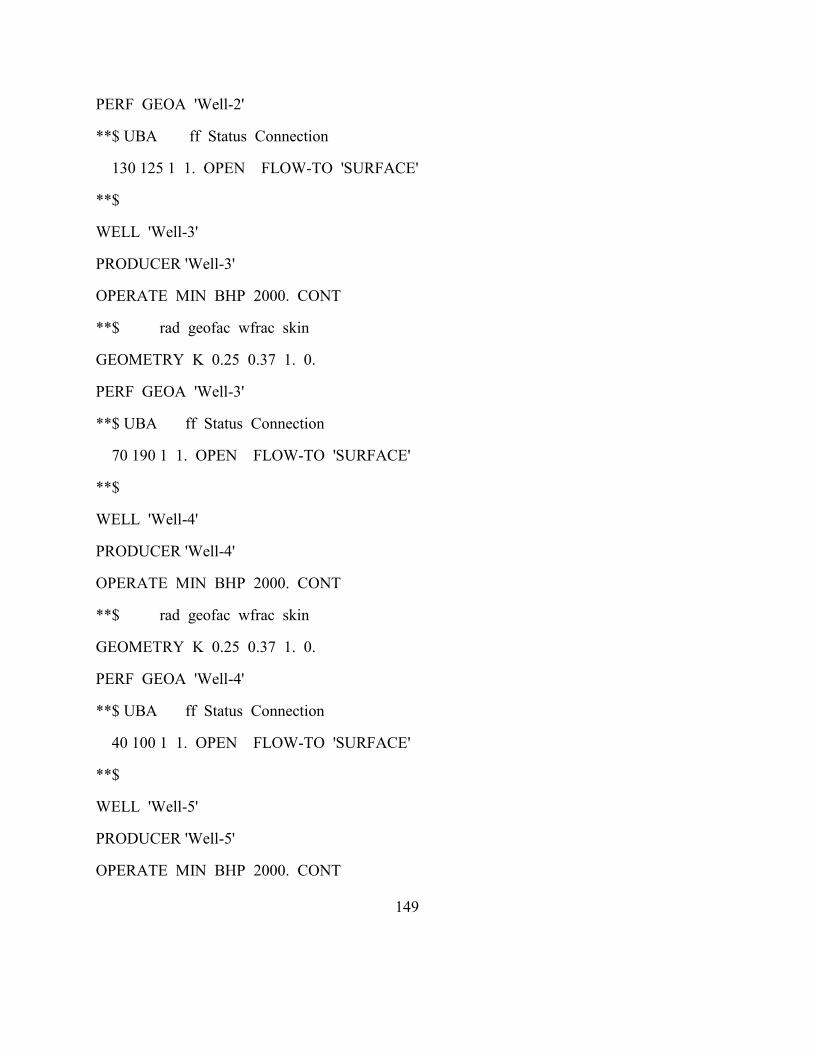
149
PERF GEOA 'Well-2'
**$ UBA ff Status Connection
130 125 1 1. OPEN FLOW-TO 'SURFACE'
**$
WELL 'Well-3'
PRODUCER 'Well-3'
OPERATE MIN BHP 2000. CONT
**$ rad geofac wfrac skin
GEOMETRY K 0.25 0.37 1. 0.
PERF GEOA 'Well-3'
**$ UBA ff Status Connection
70 190 1 1. OPEN FLOW-TO 'SURFACE'
**$
WELL 'Well-4'
PRODUCER 'Well-4'
OPERATE MIN BHP 2000. CONT
**$ rad geofac wfrac skin
GEOMETRY K 0.25 0.37 1. 0.
PERF GEOA 'Well-4'
**$ UBA ff Status Connection
40 100 1 1. OPEN FLOW-TO 'SURFACE'
**$
WELL 'Well-5'
PRODUCER 'Well-5'
OPERATE MIN BHP 2000. CONT
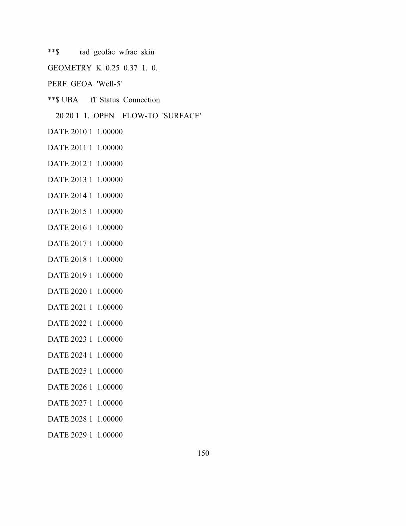
150
**$ rad geofac wfrac skin
GEOMETRY K 0.25 0.37 1. 0.
PERF GEOA 'Well-5'
**$ UBA ff Status Connection
20 20 1 1. OPEN FLOW-TO 'SURFACE'
DATE 2010 1 1.00000
DATE 2011 1 1.00000
DATE 2012 1 1.00000
DATE 2013 1 1.00000
DATE 2014 1 1.00000
DATE 2015 1 1.00000
DATE 2016 1 1.00000
DATE 2017 1 1.00000
DATE 2018 1 1.00000
DATE 2019 1 1.00000
DATE 2020 1 1.00000
DATE 2021 1 1.00000
DATE 2022 1 1.00000
DATE 2023 1 1.00000
DATE 2024 1 1.00000
DATE 2025 1 1.00000
DATE 2026 1 1.00000
DATE 2027 1 1.00000
DATE 2028 1 1.00000
DATE 2029 1 1.00000

151
STOP
A.3 RESERVOIR MODEL: 200 X 200 X 1GRID DIMENSION, 5 PRODUCTION WELLS, WELL
TESTING (CHAPTER 7)
RESULTS SIMULATOR IMEX 200900
INTERRUPT RESTART-STOP
INUNIT FIELD
WSRF WELL 1
WSRF GRID TIME
WSRF SECTOR TIME
OUTSRF WELL LAYER NONE
OUTSRF RES ALL
OUTSRF GRID BPP OILPOT PRES SO SSPRES SW WINFLUX
WPRN GRID 0
OUTPRN GRID NONE
OUTPRN RES NONE
**$ Distance units: ft
RESULTS XOFFSET 0.0000
RESULTS YOFFSET 0.0000
RESULTS ROTATION 0.0000 **$ (DEGREES)
RESULTS AXES-DIRECTIONS 1.0 -1.0 1.0

152
**$
***************************************************************************
**$ Definition of fundamental cartesian grid
**$
***************************************************************************
GRID VARI 200 200 1
KDIR DOWN
DI IVAR
200*500
DJ JVAR
200*500
DK ALL
40000*500
DTOP ALL
INCLUDE 'DTOP.INC'
**$ Property: NULL Blocks Max: 1 Min: 1
**$ 0 = null block, 1 = active block
NULL CON 1
**$ Property: Net Pay (ft) Max: 500 Min: 500
NETPAY CON 500
**$ Property: Porosity Max: 0.3 Min: 0.3
POR ALL
INCLUDE 'poro_model_5wells_sisim_well_testing.inc'
**$ Property: Permeability I (md) Max: 50 Min: 50
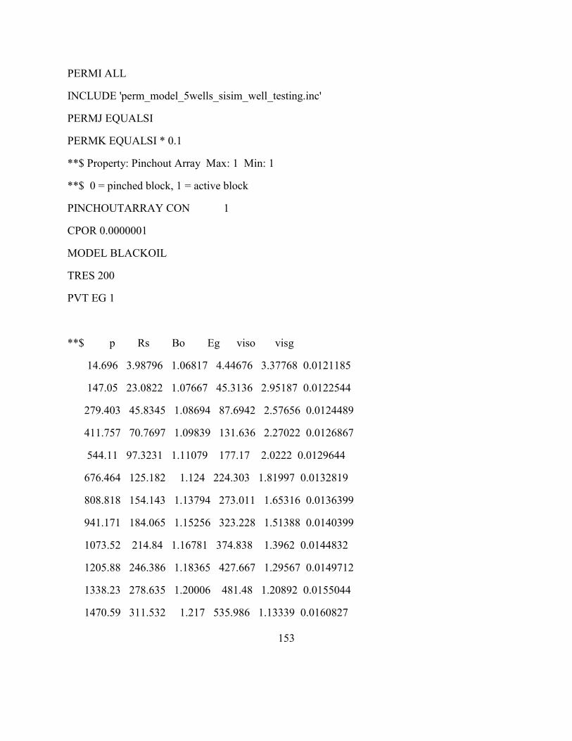
153
PERMI ALL
INCLUDE 'perm_model_5wells_sisim_well_testing.inc'
PERMJ EQUALSI
PERMK EQUALSI * 0.1
**$ Property: Pinchout Array Max: 1 Min: 1
**$ 0 = pinched block, 1 = active block
PINCHOUTARRAY CON 1
CPOR 0.0000001
MODEL BLACKOIL
TRES 200
PVT EG 1
**$ p Rs Bo Eg viso visg
14.696 3.98796 1.06817 4.44676 3.37768 0.0121185
147.05 23.0822 1.07667 45.3136 2.95187 0.0122544
279.403 45.8345 1.08694 87.6942 2.57656 0.0124489
411.757 70.7697 1.09839 131.636 2.27022 0.0126867
544.11 97.3231 1.11079 177.17 2.0222 0.0129644
676.464 125.182 1.124 224.303 1.81997 0.0132819
808.818 154.143 1.13794 273.011 1.65316 0.0136399
941.171 184.065 1.15256 323.228 1.51388 0.0140399
1073.52 214.84 1.16781 374.838 1.3962 0.0144832
1205.88 246.386 1.18365 427.667 1.29567 0.0149712
1338.23 278.635 1.20006 481.48 1.20892 0.0155044
1470.59 311.532 1.217 535.986 1.13339 0.0160827
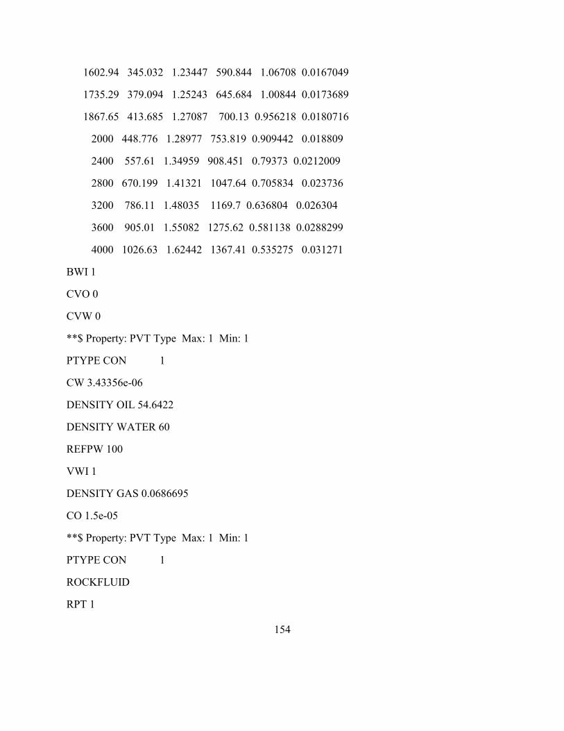
154
1602.94 345.032 1.23447 590.844 1.06708 0.0167049
1735.29 379.094 1.25243 645.684 1.00844 0.0173689
1867.65 413.685 1.27087 700.13 0.956218 0.0180716
2000 448.776 1.28977 753.819 0.909442 0.018809
2400 557.61 1.34959 908.451 0.79373 0.0212009
2800 670.199 1.41321 1047.64 0.705834 0.023736
3200 786.11 1.48035 1169.7 0.636804 0.026304
3600 905.01 1.55082 1275.62 0.581138 0.0288299
4000 1026.63 1.62442 1367.41 0.535275 0.031271
BWI 1
CVO 0
CVW 0
**$ Property: PVT Type Max: 1 Min: 1
PTYPE CON 1
CW 3.43356e-06
DENSITY OIL 54.6422
DENSITY WATER 60
REFPW 100
VWI 1
DENSITY GAS 0.0686695
CO 1.5e-05
**$ Property: PVT Type Max: 1 Min: 1
PTYPE CON 1
ROCKFLUID
RPT 1
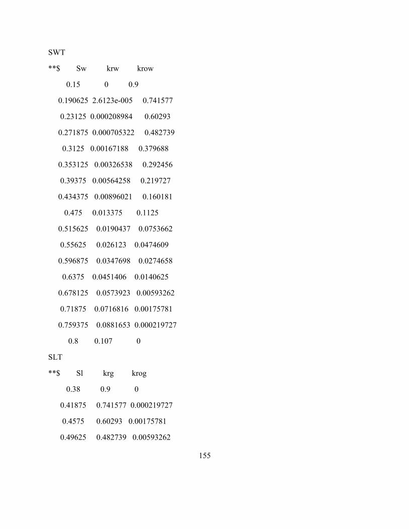
155
SWT
**$ Sw krw krow
0.15 0 0.9
0.190625 2.6123e-005 0.741577
0.23125 0.000208984 0.60293
0.271875 0.000705322 0.482739
0.3125 0.00167188 0.379688
0.353125 0.00326538 0.292456
0.39375 0.00564258 0.219727
0.434375 0.00896021 0.160181
0.475 0.013375 0.1125
0.515625 0.0190437 0.0753662
0.55625 0.026123 0.0474609
0.596875 0.0347698 0.0274658
0.6375 0.0451406 0.0140625
0.678125 0.0573923 0.00593262
0.71875 0.0716816 0.00175781
0.759375 0.0881653 0.000219727
0.8 0.107 0
SLT
**$ Sl krg krog
0.38 0.9 0
0.41875 0.741577 0.000219727
0.4575 0.60293 0.00175781
0.49625 0.482739 0.00593262

156
0.535 0.379688 0.0140625
0.57375 0.292456 0.0274658
0.6125 0.219727 0.0474609
0.65125 0.160181 0.0753662
0.69 0.1125 0.1125
0.72875 0.0753662 0.160181
0.7675 0.0474609 0.219727
0.80625 0.0274658 0.292456
0.845 0.0140625 0.379688
0.88375 0.00593262 0.482739
0.9225 0.00175781 0.60293
0.96125 0.000219727 0.741577
1 0 0.9
INITIAL
VERTICAL DEPTH_AVE WATER_OIL EQUIL
REFDEPTH 1000
REFPRES 4000
DWOC 1500
**$ Property: Bubble Point Pressure (psi) Max: 0 Min: 0
PB CON 0
NUMERICAL
RUN
DATE 2009 1 1
**$

157
WELL 'Well-1'
PRODUCER 'Well-1'
OPERATE MAX STO 100000. CONT
**$ rad geofac wfrac skin
GEOMETRY K 0.25 0.37 1. 0.
PERF GEOA 'Well-1'
**$ UBA ff Status Connection
170 50 1 1. OPEN FLOW-TO 'SURFACE'
**$
WELL 'Well-2'
PRODUCER 'Well-2'
OPERATE MIN BHP 2000. CONT
**$ rad geofac wfrac skin
GEOMETRY K 0.25 0.37 1. 0.
PERF GEOA 'Well-2'
**$ UBA ff Status Connection
130 125 1 1. OPEN FLOW-TO 'SURFACE'
**$
WELL 'Well-3'
PRODUCER 'Well-3'
OPERATE MIN BHP 2000. CONT
**$ rad geofac wfrac skin
GEOMETRY K 0.25 0.37 1. 0.
PERF GEOA 'Well-3'
**$ UBA ff Status Connection
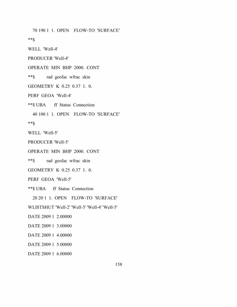
158
70 190 1 1. OPEN FLOW-TO 'SURFACE'
**$
WELL 'Well-4'
PRODUCER 'Well-4'
OPERATE MIN BHP 2000. CONT
**$ rad geofac wfrac skin
GEOMETRY K 0.25 0.37 1. 0.
PERF GEOA 'Well-4'
**$ UBA ff Status Connection
40 100 1 1. OPEN FLOW-TO 'SURFACE'
**$
WELL 'Well-5'
PRODUCER 'Well-5'
OPERATE MIN BHP 2000. CONT
**$ rad geofac wfrac skin
GEOMETRY K 0.25 0.37 1. 0.
PERF GEOA 'Well-5'
**$ UBA ff Status Connection
20 20 1 1. OPEN FLOW-TO 'SURFACE'
WLISTSHUT 'Well-2' 'Well-3' 'Well-4' 'Well-5'
DATE 2009 1 2.00000
DATE 2009 1 3.00000
DATE 2009 1 4.00000
DATE 2009 1 5.00000
DATE 2009 1 6.00000
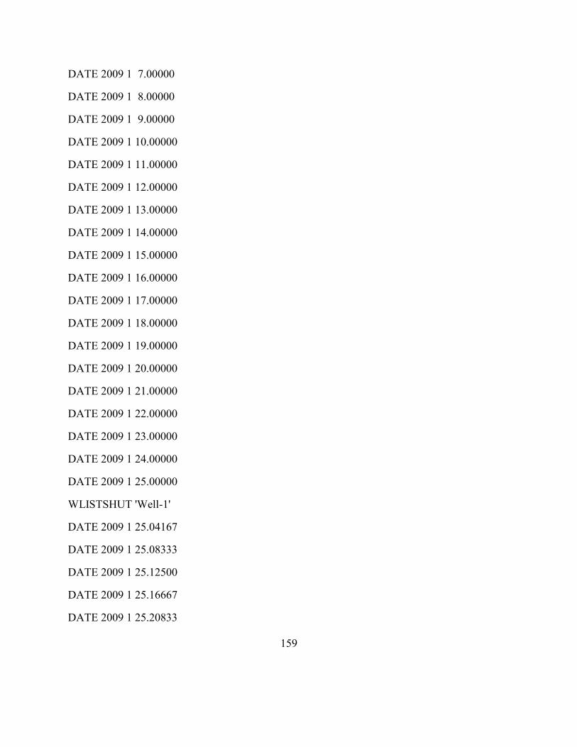
159
DATE 2009 1 7.00000
DATE 2009 1 8.00000
DATE 2009 1 9.00000
DATE 2009 1 10.00000
DATE 2009 1 11.00000
DATE 2009 1 12.00000
DATE 2009 1 13.00000
DATE 2009 1 14.00000
DATE 2009 1 15.00000
DATE 2009 1 16.00000
DATE 2009 1 17.00000
DATE 2009 1 18.00000
DATE 2009 1 19.00000
DATE 2009 1 20.00000
DATE 2009 1 21.00000
DATE 2009 1 22.00000
DATE 2009 1 23.00000
DATE 2009 1 24.00000
DATE 2009 1 25.00000
WLISTSHUT 'Well-1'
DATE 2009 1 25.04167
DATE 2009 1 25.08333
DATE 2009 1 25.12500
DATE 2009 1 25.16667
DATE 2009 1 25.20833

160
DATE 2009 1 25.25000
DATE 2009 1 25.29167
DATE 2009 1 25.33333
DATE 2009 1 25.37500
DATE 2009 1 25.41667
DATE 2009 1 25.45833
DATE 2009 1 25.50000
DATE 2009 1 25.54167
DATE 2009 1 25.58333
DATE 2009 1 25.62500
DATE 2009 1 25.66667
DATE 2009 1 25.70833
DATE 2009 1 25.75000
DATE 2009 1 25.79167
DATE 2009 1 25.83333
DATE 2009 1 25.87500
DATE 2009 1 25.91667
DATE 2009 1 25.95833
DATE 2009 1 26.00000
DATE 2009 1 26.04167
DATE 2009 1 26.08333
DATE 2009 1 26.12500
DATE 2009 1 26.16667
DATE 2009 1 26.20833
DATE 2009 1 26.25000

161
DATE 2009 1 26.29167
DATE 2009 1 26.33333
DATE 2009 1 26.37500
DATE 2009 1 26.41667
DATE 2009 1 26.45833
DATE 2009 1 26.50000
DATE 2009 1 26.54167
DATE 2009 1 26.58333
DATE 2009 1 26.62500
DATE 2009 1 26.66667
DATE 2009 1 26.70833
DATE 2009 1 26.75000
DATE 2009 1 26.79167
DATE 2009 1 26.83333
DATE 2009 1 26.87500
DATE 2009 1 26.91667
DATE 2009 1 26.95833
DATE 2009 1 27.00000
DATE 2009 1 27.04167
DATE 2009 1 27.08333
DATE 2009 1 27.12500
DATE 2009 1 27.16667
DATE 2009 1 27.20833
DATE 2009 1 27.25000
DATE 2009 1 27.29167

162
DATE 2009 1 27.33333
DATE 2009 1 27.37500
DATE 2009 1 27.41667
DATE 2009 1 27.45833
DATE 2009 1 27.50000
DATE 2009 1 27.54167
DATE 2009 1 27.58333
DATE 2009 1 27.62500
DATE 2009 1 27.66667
DATE 2009 1 27.70833
DATE 2009 1 27.75000
DATE 2009 1 27.79167
DATE 2009 1 27.83333
DATE 2009 1 27.87500
DATE 2009 1 27.91667
DATE 2009 1 27.95833
DATE 2009 1 28.00000
DATE 2009 1 28.04167
DATE 2009 1 28.08333
DATE 2009 1 28.12500
DATE 2009 1 28.16667
DATE 2009 1 28.20833
DATE 2009 1 28.25000
DATE 2009 1 28.29167
DATE 2009 1 28.33333
163
DATE 2009 1 28.37500
DATE 2009 1 28.41667
DATE 2009 1 28.45833
DATE 2009 1 28.50000
DATE 2009 1 28.54167
DATE 2009 1 28.58333
DATE 2009 1 28.62500
DATE 2009 1 28.66667
DATE 2009 1 28.70833
DATE 2009 1 28.75000
DATE 2009 1 28.79167
DATE 2009 1 28.83333
DATE 2009 1 28.87500
DATE 2009 1 28.91667
DATE 2009 1 28.95833
DATE 2009 1 29.00000
DATE 2009 1 29.04167
DATE 2009 1 29.08333
DATE 2009 1 29.12500
DATE 2009 1 29.16667
DATE 2009 1 29.20833
DATE 2009 1 29.25000
DATE 2009 1 29.29167
DATE 2009 1 29.33333
DATE 2009 1 29.37500

164
DATE 2009 1 29.41667
DATE 2009 1 29.45833
DATE 2009 1 29.50000
DATE 2009 1 29.54167
DATE 2009 1 29.58333
DATE 2009 1 29.62500
DATE 2009 1 29.66667
DATE 2009 1 29.70833
DATE 2009 1 29.75000
DATE 2009 1 29.79167
DATE 2009 1 29.83333
DATE 2009 1 29.87500
DATE 2009 1 29.91667
DATE 2009 1 29.95833
DATE 2009 1 30.00000
DATE 2009 1 30.04167
DATE 2009 1 30.08333
DATE 2009 1 30.12500
DATE 2009 1 30.16667
DATE 2009 1 30.20833
DATE 2009 1 30.25000
DATE 2009 1 30.29167
DATE 2009 1 30.33333
DATE 2009 1 30.37500
DATE 2009 1 30.41667

165
DATE 2009 1 30.45833
DATE 2009 1 30.50000
DATE 2009 1 30.54167
DATE 2009 1 30.58333
DATE 2009 1 30.62500
DATE 2009 1 30.66667
DATE 2009 1 30.70833
DATE 2009 1 30.75000
DATE 2009 1 30.79167
DATE 2009 1 30.83333
DATE 2009 1 30.87500
DATE 2009 1 30.91667
DATE 2009 1 30.95833
DATE 2009 1 31.00000
DATE 2009 1 31.04167
DATE 2009 1 31.08333
DATE 2009 1 31.12500
DATE 2009 1 31.16667
DATE 2009 1 31.20833
DATE 2009 1 31.25000
DATE 2009 1 31.29167
DATE 2009 1 31.33333
DATE 2009 1 31.37500
DATE 2009 1 31.41667
DATE 2009 1 31.45833

166
DATE 2009 1 31.50000
DATE 2009 1 31.54167
DATE 2009 1 31.58333
DATE 2009 1 31.62500
DATE 2009 1 31.66667
DATE 2009 1 31.70833
DATE 2009 1 31.75000
DATE 2009 1 31.79167
DATE 2009 1 31.83333
DATE 2009 1 31.87500
DATE 2009 1 31.91667
DATE 2009 1 31.95833
DATE 2009 2 1.00000
DATE 2009 2 1.04167
DATE 2009 2 1.08333
DATE 2009 2 1.12500
DATE 2009 2 1.16667
DATE 2009 2 1.20833
DATE 2009 2 1.25000
DATE 2009 2 1.29167
DATE 2009 2 1.33333
DATE 2009 2 1.37500
DATE 2009 2 1.41667
DATE 2009 2 1.45833
DATE 2009 2 1.50000

167
DATE 2009 2 1.54167
DATE 2009 2 1.58333
DATE 2009 2 1.62500
DATE 2009 2 1.66667
DATE 2009 2 1.70833
DATE 2009 2 1.75000
DATE 2009 2 1.79167
DATE 2009 2 1.83333
DATE 2009 2 1.87500
DATE 2009 2 1.91667
DATE 2009 2 1.95833
DATE 2009 2 2.00000
STOP
168
Appendix B: MatLab Codes to Perform General Operations
The work in this thesis required working with hundreds of realizations of reservoir properties,
and syncing those multiple realizations among CMG-IMEX, SGeMS, and MatLab. This
appendix presents various MatLab codes written as general functions which were used in this
thesis.
B.1 IMPORTING DATA FROM GSLIB FORMAT FILES TO MATLAB
function
[property_as_mat_nModels_want,property_as_mat_all_nModels]=gslib_file_to_mat_g
eneral(nModel,nCell,nModel_want,gslib_file_name) % must enter the last
argument, gslib_file_name, in single quotes as its treated as a string
%% making third argument optional, otherwise if entered should be in string
format
if nargin<3, %(code to be executed even when only 2 arguments are provided)
gslib_file_name=input('Enter the gslib file name: ','s');
end
if ~ischar(gslib_file_name)
error('gslib_file_name should a be string');
169
end
if length(gslib_file_name)<4 || ~strcmpi(gslib_file_name(end-3:end),'.dat'),
gslib_file_name=[gslib_file_name '.dat']; % string concatenation
end
%% Reading directly from the .dat files generated from SGEMS and making the
data of file as a variable
property_gslib_format=textread(gslib_file_name,'%f\t','headerlines',nModel+2);
property_as_mat_all_nModels=reshape(property_gslib_format,nModel,nCell)';
property_as_mat_nModels_want=property_as_mat_all_nModels(:,1:nModel_want); %
Note: 'nModel_want' instead of 'nModel'
B.2 MAKING A DATA FILE WITH GSLIB FORMAT FROM MATLAB WORKSPACE
function
[]=write_property_to_gslib_file_general(nModel,name_of_gslib_file_want,header_
property_name_want,property_as_gslib_want)
if ~ischar(name_of_gslib_file_want)||~ischar(header_property_name_want)
error('name_of_gslib_file_want and header_property_name_want should a be
string');
end
170
%# open the file
name_of_gslib_file_want=[name_of_gslib_file_want '.dat'];
fid = fopen(name_of_gslib_file_want,'w');
%# start writing. First line: title
fprintf(fid,'%s\n',header_property_name_want); %# don't forget \n for newline.
Use \n\r if yow want to open this in notepad
%# write number of models
fprintf(fid,'%i\n',nModel)
%# loop to write the rest of the header
for iModel = 1:nModel
fprintf(fid,'%s_%i\n',header_property_name_want,iModel);
end
%# use your favorite method to write the rest of the data.
%# for example, you could use fprintf again, using \t to add tabs
%# create format-string
%# check the help to fprintf to learn about formatting details
formatString = repmat('%f\t',1,nModel);
formatString = [formatString(1:end-1),'n']; %# replace last tab with newline
%# transpose the array, because fprintf reshapes the array to a vector and

171
%# 'fills' the format-strings sequentially until it runs out of data
fprintf(fid,formatString,property_as_gslib_want');
%# close the file
fclose(fid);
B.3 CALLING CMG-IMEX FROM MATLAB TO RETRIEVE BOTTOM HOLE PRESSURE (BHP)
DATA
function
[timesteps_days_BHP,BHP_w1,BHP_w2,BHP_w4,BHP_w5]=BHP_from_CMG_general(nModel,n
Cell,nModel_want,ReservoirModel_CMGBuilder,poro_models_gslib_file,perm_models_
gslib_file,poro_model_inc_file,perm_model_inc_file,ReportBHP)
ReservoirModel_CMGBuilder_dat=[ReservoirModel_CMGBuilder '.dat']; % string
concatenation
%# poro and perm models extracted from gslib files and made into matlab
variable
poro_models=gslib_file_to_mat_general(nModel,nCell,nModel_want,poro_models_gsl
ib_file);
perm_models=gslib_file_to_mat_general(nModel,nCell,nModel_want,perm_models_gsl
ib_file);

172
%# poro and perm model '.inc' files
poro_model_inc=[poro_model_inc_file '.inc'];
perm_model_inc=[perm_model_inc_file '.inc'];
%# Report files for BHP, input and output, for CMG
ReportBHP_rwd=[ReportBHP '.rwd'];
ReportBHP_rwo=[ReportBHP '.rwo'];
%% loop to run all nModel
for model_no=1:nModel_want
%% Writing the porosity and permeability model one at a time in .inc file,
which will be read and will work as input to porosity and permeability models
in CMG
dlmwrite(poro_model_inc,poro_models(:,model_no)/100,'delimiter','\n');
dlmwrite(perm_model_inc,perm_models(:,model_no),'delimiter','\n');
%% Calling mx201010.exe and running report.exe from CMG portal
%# Calls CMG
[status_mx201010,result_mx201010]=system(['mx201010.exe -f '
ReservoirModel_CMGBuilder_dat '']);

173
%# Calls parameter report file and generates output file
[status_report,result_report]=system(['report.exe /f "' ReportBHP_rwd '"
/o "' ReportBHP_rwo '"']);
%% Reading and writing the BHP results using .rwd and .rwo files
%# open the ReportBHP_rwo file
fid = fopen(ReportBHP_rwo);
%# read it into one big array, row by row
fileContents = textscan(fid,'%s','Delimiter','\n');
fileContents = fileContents{1};
fclose(fid); %# don't forget to close the file again
%# find rows containing TABLE NUMBER
wellStarts = strmatch('TABLE NUMBER',fileContents);
nWells = length(wellStarts);
%# loop through the wells and read the numeric data
wellStarts = [wellStarts];
nT_BHP=wellStarts(2)-wellStarts(1)-5;
for w = 1:nWells
%# read lines containing numbers

174
tmp = fileContents(wellStarts(w)+5:wellStarts(w)+4+nT_BHP);
%# convert strings to numbers
tmp = cellfun(@str2num,tmp,'uniformOutput',false);
%# catenate array
tmp = cat(1,tmp{:});
%# assign output
BHP_w(:,w)=tmp(:,2);
end
timesteps_days_BHP=tmp(:,1);
BHP_w1(model_no,:)=BHP_w(:,1);
BHP_w2(model_no,:)=BHP_w(:,2);
BHP_w3(model_no,:)=BHP_w(:,3);
BHP_w4(model_no,:)=BHP_w(:,4);
BHP_w5(model_no,:)=BHP_w(:,5);
end % end of the mail loop for running different models
B.4 CALLING CMG-IMEX FROM MATLAB TO RETRIEVE PRODUCTION RATE DATA
function
[q_yearly]=q_from_CMG_general(nModel,nCell,nModel_want,T,ReservoirModel_CMGBui
lder,poro_models_gslib_file,perm_models_gslib_file,poro_model_inc_file,perm_mo
del_inc_file,Reportq)
175
ReservoirModel_CMGBuilder_dat=[ReservoirModel_CMGBuilder '.dat']; % string
concatenation
%# poro and perm models extracted from gslib files and made into matlab
variable
poro_models=gslib_file_to_mat_general(nModel,nCell,nModel_want,poro_models_gsl
ib_file);
perm_models=gslib_file_to_mat_general(nModel,nCell,nModel_want,perm_models_gsl
ib_file);
%# poro and perm model '.inc' files
poro_model_inc=[poro_model_inc_file '.inc'];
perm_model_inc=[perm_model_inc_file '.inc'];
%# Report files for q, input and output, for CMG
Reportq_rwd=[Reportq '.rwd'];
Reportq_rwo=[Reportq '.rwo'];
%% loop to run all nModel
for model_no=1:nModel_want
%% Writing the porosity and permeability model one at a time in .inc file,
which will be read and will work as input to porosity and permeability models
in CMG

176
dlmwrite(poro_model_inc,poro_models(:,model_no)/100,'delimiter','\n');
dlmwrite(perm_model_inc,perm_models(:,model_no),'delimiter','\n');
%% Calling mx201010.exe and running report.exe from CMG portal
%# Calls CMG
[status_mx201010,result_mx201010]=system(['mx201010.exe -f '
ReservoirModel_CMGBuilder_dat '']); % Calls CMG
%# Calls parameter report file and generates output file
[status_report,result_report]=system(['report.exe /f "' Reportq_rwd '" /o
"' Reportq_rwo '"']);
%% Reading and writing the q results using .rwd and .rwo files
%# open the Reportq_rwo file
fid = fopen(Reportq_rwo);
%# read it into one big array, row by row
fileContents = textscan(fid,'%s','Delimiter','\n');
fileContents = fileContents{1};
fclose(fid); %# don't forget to close the file again
%# find rows containing TABLE NUMBER
177
wellStarts = strmatch('TABLE NUMBER',fileContents);
nWells = length(wellStarts);
%# loop through the wells and read the numeric data
wellData = cell(nWells,2);
wellStarts = [wellStarts;length(fileContents)];
for w = 1:nWells
%# read lines containing numbers
tmp = fileContents(wellStarts(w)+6:wellStarts(w)+6+T-1);
%# convert strings to numbers
tmp = cellfun(@str2num,tmp,'uniformOutput',false);
%# catenate array
tmp = cat(1,tmp{:});
%# assign output
q_yearly_w(:,w)=tmp(:,2);
end
q_yearly(model_no,:)=(365.*sum(q_yearly_w,2));
end % end of the mail loop for running different models
B.5 COMPUTING PRODUCTION RATE THROUGH DECLINE CURVE ANALYSIS
%% PRODUCTION DATA COMPUTED USING TANK METHOD EQUATIONS
178
function[q_MethodType]=q_from_TankMethod_general(nModel,nCell,nModel_want,A,Nw
,rw,CA,skin,mu,h,ct,Pi,Pwf,Bo,T,xy_wells,poro_models_gslib_file,perm_models_gs
lib_file)
poro_models=gslib_file_to_mat_general(nModel,nCell,nModel_want,poro_models_gsl
ib_file);
perm_models=gslib_file_to_mat_general(nModel,nCell,nModel_want,perm_models_gsl
ib_file);
Aw=A./Nw; % Area of drainage of 1 well. It is not A./6, because the 6th well
is not producing.
%% Mean of Poro and Perm
for model_no=1:nModel_want
phi_mean(model_no)=mean(poro_models(:,model_no))/100;
k=reshape(perm_models(:,model_no),sqrt(nCell),sqrt(nCell))';
% Limit the well perm values taken around the wells to [0,sqrt(nCell)]
xy_wells_limit1=(xy_wells-5<0);
xy_wells_limit2=(xy_wells+5>sqrt(nCell));
xy_wells(xy_wells_limit1)=xy_wells(xy_wells_limit1)+5;
xy_wells(xy_wells_limit2)=sqrt(nCell)-5;

179
%# mean value of permeability is taken as mean of 10 perm values in X and
Y direction around each well
k_mean(model_no)=(mean(mean(k(xy_wells(1,1)-
5:xy_wells(1,1)+5,xy_wells(2,1)-
5:xy_wells(2,1)+5)))+mean(mean(k(xy_wells(1,2)-
5:xy_wells(1,2)+5,xy_wells(2,2)-
5:xy_wells(2,2)+5)))+mean(mean(k(xy_wells(1,3)-
5:xy_wells(1,3)+5,xy_wells(2,3)-
5:xy_wells(2,3)+5)))+mean(mean(k(xy_wells(1,4)-
5:xy_wells(1,4)+5,xy_wells(2,4)-
5:xy_wells(2,4)+5)))+mean(mean(k(xy_wells(1,5)-
5:xy_wells(1,5)+5,xy_wells(2,5)-5:xy_wells(2,5)+5))))./5;
end
%% PRODUCTION AT DIFFERENT YEARS FOR 5 WELLS
for j=1:T % Number of year
t(j)=j;
for model_no=1:nModel_want % number of models or realizations
Jk(model_no)=(0.00708*h*k_mean(model_no))/(mu*((0.5*log(Aw/((rw^2)*CA)))+5.75+
skin)); % well productivity index
Vp(model_no)=7757.792*A.*h.*phi_mean(model_no); % pore volume
lambda(model_no)=(365*Nw*Jk(model_no))./(Vp(model_no)*ct); % decay
rate of the field
180
% Pi_explorwell(model_no,j)=((Pi-Pwf)*exp(-
lambda(model_no).*t(j)))+Pwf; % new intial pressure at end of year t(j)
q_osci(model_no)=(Nw*Jk(model_no)*(Pi-Pwf))/Bo; % intial producing
rate for entire field
Np(model_no,j)=(365*(q_osci(model_no)./lambda(model_no))).*(1-exp(-
lambda(model_no).*t(j))); % cumulative oil production by 5 wells for t(j)
years starting year 0 prior to drilling an exploratory well
if j>1
q_MethodType(model_no,j)=Np(model_no,j)-Np(model_no,j-1); % oil
production by 5 wells for individual year t(j) prior to drilling an
exploratory well
else
q_MethodType(model_no,j)=Np(model_no,j); % oil production by 5
wells for individual year 1 prior to drilling an exploratory well
end
end % end of number of models or realizations for any single year
end
B.6 PV, NPV AND ROV ANALYSIS
function [PV,NPV,ROV,q_MethodType,volatility_LR_sum_PV,volatility_LR_sum_NPV]
=
PV_and_ROV_analysis_general(nModel,nCell,nModel_want,r,p_oil,A,Nw,rw,CA,skin,m
u,h,ct,Pi,Pwf,Bo,T,opex,capex,xy_wells,poro_models_gslib_file,perm_models_gsli
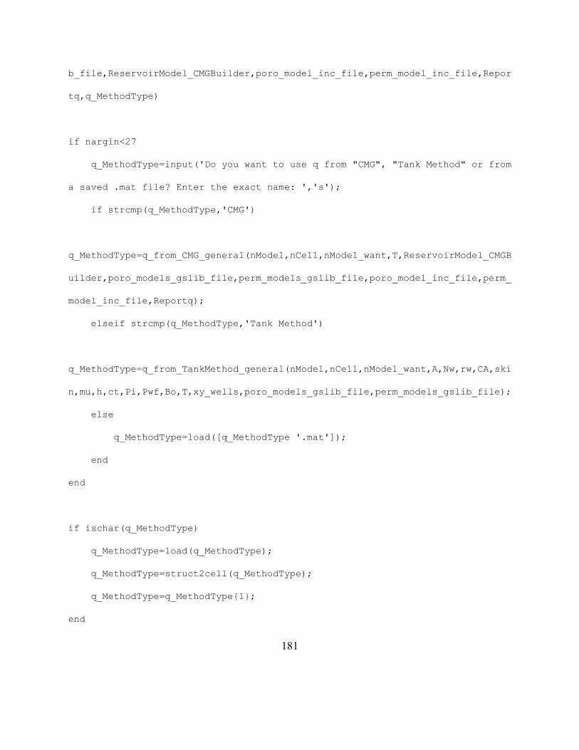
181
b_file,ReservoirModel_CMGBuilder,poro_model_inc_file,perm_model_inc_file,Repor
tq,q_MethodType)
if nargin<27
q_MethodType=input('Do you want to use q from "CMG", "Tank Method" or from
a saved .mat file? Enter the exact name: ','s');
if strcmp(q_MethodType,'CMG')
q_MethodType=q_from_CMG_general(nModel,nCell,nModel_want,T,ReservoirModel_CMGB
uilder,poro_models_gslib_file,perm_models_gslib_file,poro_model_inc_file,perm_
model_inc_file,Reportq);
elseif strcmp(q_MethodType,'Tank Method')
q_MethodType=q_from_TankMethod_general(nModel,nCell,nModel_want,A,Nw,rw,CA,ski
n,mu,h,ct,Pi,Pwf,Bo,T,xy_wells,poro_models_gslib_file,perm_models_gslib_file);
else
q_MethodType=load([q_MethodType '.mat']);
end
end
if ischar(q_MethodType)
q_MethodType=load(q_MethodType);
q_MethodType=struct2cell(q_MethodType);
q_MethodType=q_MethodType{1};
end
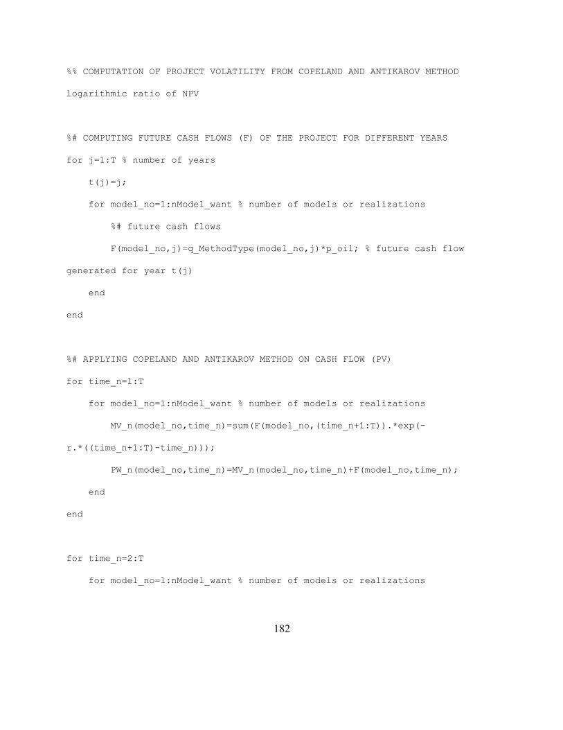
182
%% COMPUTATION OF PROJECT VOLATILITY FROM COPELAND AND ANTIKAROV METHOD
logarithmic ratio of NPV
%# COMPUTING FUTURE CASH FLOWS (F) OF THE PROJECT FOR DIFFERENT YEARS
for j=1:T % number of years
t(j)=j;
for model_no=1:nModel_want % number of models or realizations
%# future cash flows
F(model_no,j)=q_MethodType(model_no,j)*p_oil; % future cash flow
generated for year t(j)
end
end
%# APPLYING COPELAND AND ANTIKAROV METHOD ON CASH FLOW (PV)
for time_n=1:T
for model_no=1:nModel_want % number of models or realizations
MV_n(model_no,time_n)=sum(F(model_no,(time_n+1:T)).*exp(-
r.*((time_n+1:T)-time_n)));
PW_n(model_no,time_n)=MV_n(model_no,time_n)+F(model_no,time_n);
end
end
for time_n=2:T
for model_no=1:nModel_want % number of models or realizations
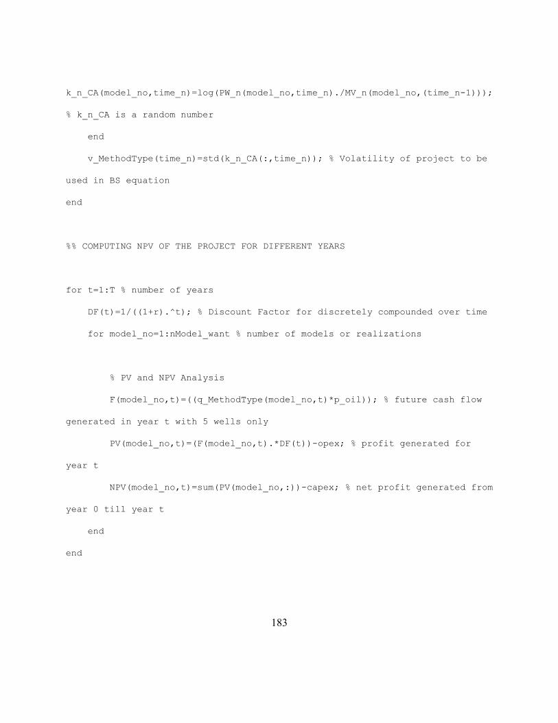
183
k_n_CA(model_no,time_n)=log(PW_n(model_no,time_n)./MV_n(model_no,(time_n-1)));
% k_n_CA is a random number
end
v_MethodType(time_n)=std(k_n_CA(:,time_n)); % Volatility of project to be
used in BS equation
end
%% COMPUTING NPV OF THE PROJECT FOR DIFFERENT YEARS
for t=1:T % number of years
DF(t)=1/((1+r).^t); % Discount Factor for discretely compounded over time
for model_no=1:nModel_want % number of models or realizations
% PV and NPV Analysis
F(model_no,t)=((q_MethodType(model_no,t)*p_oil)); % future cash flow
generated in year t with 5 wells only
PV(model_no,t)=(F(model_no,t).*DF(t))-opex; % profit generated for
year t
NPV(model_no,t)=sum(PV(model_no,:))-capex; % net profit generated from
year 0 till year t
end
end
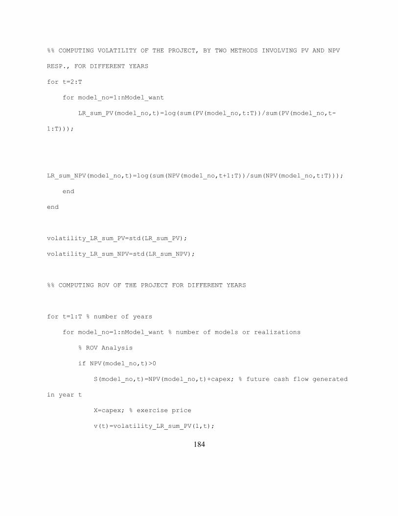
184
%% COMPUTING VOLATILITY OF THE PROJECT, BY TWO METHODS INVOLVING PV AND NPV
RESP., FOR DIFFERENT YEARS
for t=2:T
for model_no=1:nModel_want
LR_sum_PV(model_no,t)=log(sum(PV(model_no,t:T))/sum(PV(model_no,t-
1:T)));
LR_sum_NPV(model_no,t)=log(sum(NPV(model_no,t+1:T))/sum(NPV(model_no,t:T)));
end
end
volatility_LR_sum_PV=std(LR_sum_PV);
volatility_LR_sum_NPV=std(LR_sum_NPV);
%% COMPUTING ROV OF THE PROJECT FOR DIFFERENT YEARS
for t=1:T % number of years
for model_no=1:nModel_want % number of models or realizations
% ROV Analysis
if NPV(model_no,t)>0
S(model_no,t)=NPV(model_no,t)+capex; % future cash flow generated
in year t
X=capex; % exercise price
v(t)=volatility_LR_sum_PV(1,t);
185
d1(model_no,t)=(log(S(model_no,t)/X)+(r+v(t).^2/2)*(t))./(v(t).*sqrt(t));
d2(model_no,t)=d1(model_no,t)-v(t).*sqrt(t);
ROV(model_no,t)=(S(model_no,t).*normcdf(d1(model_no,t)))-(X.*exp(-
r*(t)).*normcdf(d2(model_no,t)));
else
ROV(model_no,t)=0;
end
if ROV(model_no,t)<0
ROV(model_no,t)=0;
end
end
end
B.7 NPV AND RESERVE ESTIMATION BY STOOIP
function
[NPV_by_STOOIP,P10,P25,P50,P75,P90,vol_reserve]=NPV_reserve_by_STOOIP(nModel,n
Model_want,nCell,poro_models_gslib_format,Sw) % Sw has to be in percentage
p_oil=70; % $/STB
%% Changing co-ordinate system from SGEMS to CMG
186
%# Calling function 'gslib_file_to_mat_general.mat' to convert property values
from gslib format to matlab format
if ischar(poro_models_gslib_format)==1
[poro_as_mat_nModels_want,poro_as_mat_all_nModels]=gslib_file_to_mat_general(n
Model,nCell,nModel_want,poro_models_gslib_format);
else
poro_as_mat_nModels_want=poro_models_gslib_format;
end
if nargin<5, %(code to be executed even when only 4 arguments are provided)
Sw_all_nModels=load('Swav_seismic_yearly_CMG');
Sw_all_nModels=struct2cell(Sw_all_nModels);
Sw_all_nModels=Sw_all_nModels{1};
Sw_all_nModels=mean(Sw_all_nModels(2:21,:));
Sw=mean(Sw_all_nModels);
end
%% Calculating Stock Tank Original Oil in Place (STOOIP)
% Formula for OOIP: N [in stb]=6.2898*(Vb*phi*(1-Sw))/Boi); 6.289808 is
% used to convert 'N' in cubic metres to stb Area of one cell is 500ft x
% 500ft, and paythickness is uniformly 500ft.
for model_no=1:nModel_want

187
N(:,model_no)=((((50*500*50*500*1*500)/(3.28^3))*(poro_as_mat_nModels_want(:,m
odel_no)/100)*(1-(Sw/100)))/1.54)*6.2898;
STOOIP(model_no)=sum(N(:,model_no)); % Adding the 'N' for all the cells
gives STOOIP
end
%% RECOVERY FACTOR (Rf) AND VOLUMETRIC VALUE OF THE RESERVE
% Formula for Recovery Factor: Rf [in fraction]=(Swav-Swirr)/(1-Swirr),
% where Swirr = 0.10
Rf=((Sw/100)-0.10)/(1-0.10);
%# Volumeteric Value of the Reserve
vol_reserve=Rf.*STOOIP; % in STB
NPV_by_STOOIP=vol_reserve*p_oil; % in $
percentiles=prctile(NPV_by_STOOIP,[10,25,50,75,90]);
P90=percentiles(1);
P75=percentiles(2);
P50=percentiles(3);
P25=percentiles(4);
P10=percentiles(5);

188
B.8 BLOV ANLYSIS
function
[price,BLOV_lattice,underlying_lattice]=BLOV_general(S0,K,sigma,r,T,nColumn,ti
tle_of_option_lattice,title_of_underlying_lattice)
% BLOV stands for Binomial Lattice Option Valuation
%% Check if the title_of_lattice is in string format
if nargin==8
if ~ischar(title_of_option_lattice) &&
~ischar(title_of_underlying_lattice)
error('title_of_option_lattice and title_of_underlying_lattice should
a be string');
end
elseif nargin==7
if ~ischar(title_of_option_lattice)
error('title_of_option_lattice should a be string');
end
end
%% Constant parameters
del_T=T./nColumn; % where n is the number of columns in binomial lattice
u=exp(sigma.*sqrt(del_T));
d=1./u;
189
p=(exp(r.*del_T)-d)./(u-d);
a=exp(-r.*del_T);
%% Initializing the lattice
Stree=zeros(nColumn+1,nColumn+1);
BLOV_lattice=zeros(nColumn+1,nColumn+1);
%% FORWARD INDUCTION
for i=0:nColumn
for j=0:i
Stree(j+1,i+1)=S0.*(u.^(i-j))*(d.^j);
end
end
underlying_lattice=Stree(:,i+1);
for i=0:nColumn
BLOV_lattice(i+1,nColumn+1)=max(Stree(i+1,nColumn+1)-K,0);
end
%# Draw the lattice of the underlying asset only if asked in the function
argument
if nargin>7

190
%# Drawing the binomial lattice for the underlying asset
N = size(Stree,1);
[xPoints,yPoints] = meshgrid(0:N-1);
yPoints = bsxfun(@plus,-yPoints,0:0.5:(N-0.5)/2);
xLines = [xPoints([1:N+1:N^2-N-1 1:N:N^2-2*N+1]); ...
xPoints([1:N-1 N:-1:2],N).']; %'
yLines = [yPoints([1:N+1:N^2-N-1 1:N:N^2-2*N+1]); ...
yPoints([1:N-1 N:-1:2],N).']; %'
index = find(triu(reshape(1:N^2,N,N)));
xPoints = xPoints(index);
yPoints = yPoints(index);
values = strtrim(cellstr(num2str(Stree(index),'%1.4e')));
%# Create the figure
hFigure = figure('Color','w');
hAxes = axes('Parent',hFigure,'XLim',[-0.5 N-0.5],...
'YLim',[min(yPoints)-0.5 max(yPoints)+0.5],...
'YColor','w','XTick',0:N-1,'LineWidth',2);
set(hAxes,'XTickLabel',linspace(0,T,N).');
hold on;
plot(hAxes,xLines,yLines,'k','LineWidth',2);
plot(hAxes,xPoints,yPoints,'o','MarkerFaceColor',[0.96 0.96 0.86],...
'MarkerSize',60,'MarkerEdgeColor','k','LineWidth',2);
191
text(xPoints,yPoints,values,'Parent',hAxes,...
'HorizontalAlignment','center');
xlabel(['Number of steps to ', num2str(T), ' years'])
ylabel('Probability Distribution of Underlying Asset in USD','Color','k')
title(title_of_underlying_lattice,'Fontweight','Bold')
hold off;
end
%% BACKWARD INDUCTION
for i=nColumn:-1:1
for j=0:i-1
BLOV_lattice(j+1,i)=a.*(((1-
p).*BLOV_lattice(j+2,i+1))+(p.*BLOV_lattice(j+1,i+1)));
end
end
price=BLOV_lattice(1,1);
%# Draw the option lattice only if asked in the function argument
if nargin>6
%# Drawing the binomial lattice for the option
N = size(BLOV_lattice,1);
192
[xPoints,yPoints] = meshgrid(0:N-1);
yPoints = bsxfun(@plus,-yPoints,0:0.5:(N-0.5)/2);
xLines = [xPoints([1:N+1:N^2-N-1 1:N:N^2-2*N+1]); ...
xPoints([1:N-1 N:-1:2],N).']; %'
yLines = [yPoints([1:N+1:N^2-N-1 1:N:N^2-2*N+1]); ...
yPoints([1:N-1 N:-1:2],N).']; %'
index = find(triu(reshape(1:N^2,N,N)));
xPoints = xPoints(index);
yPoints = yPoints(index);
values = strtrim(cellstr(num2str(BLOV_lattice(index),'%1.4e')));
%# Create the figure
hFigure = figure('Color','w');
hAxes = axes('Parent',hFigure,'XLim',[-0.5 N-0.5],...
'YLim',[min(yPoints)-0.5 max(yPoints)+0.5],...
'YColor','w','XTick',0:N-1,'LineWidth',2);
set(hAxes,'XTickLabel',linspace(0,T,N).');
hold on;
plot(hAxes,xLines,yLines,'k','LineWidth',2);
plot(hAxes,xPoints,yPoints,'o','MarkerFaceColor',[0.96 0.96 0.86],...
'MarkerSize',60,'MarkerEdgeColor','k','LineWidth',2);
text(xPoints,yPoints,values,'Parent',hAxes,...
'HorizontalAlignment','center');
xlabel(['Number of steps to ', num2str(T), ' years'])
193
ylabel('Probability Distribution of Option Values in USD','Color','k')
title(title_of_option_lattice,'Fontweight','Bold')
hold off;
end
%% Converting the lattice of upper traingular matrix to a tree format
N = size(BLOV_lattice,1); %# The size of the rows and columns in BLOV_lattice
BLOV_lattice = full(spdiags(spdiags(BLOV_lattice),(1-N):2:(N-1),zeros(2*N-
1,N)));
B.9 CALLING GSLIB EXECUTABLE ‘TRANS’ FROM MATLAB AND RETRIEVING THE
RESULTANT DATA
function
[transformed_property_as_gslib,property_as_mat_all_models,result]=generate_dat
a_after_trans_general(nModel,nCell,nModel_want,property_models_gslib_file,prop
erty_model_inc_file,transformed_file_out,name_of_gslib_file_want,name_of_heade
r_want)
[property_models_mat,property_as_mat_all_models]=gslib_file_to_mat_general(nMo
del,nCell,nModel_want,property_models_gslib_file);
%# property model '.inc' file
property_model_inc=[property_model_inc_file '.inc'];
194
transformed_file_name_out=[transformed_file_out '.out'];
%% loop to run all nModel
for model_no=1:nModel_want
prefixData = property_model_inc_file;
%# write header lines to file
fid = fopen(property_model_inc, 'wt');
fprintf(fid,'%s\n',prefixData); %# don't forget \n for newline. Use \n\r
if yow want to open this in notepad
fprintf(fid,'%i\n',1)
fprintf(fid,'%s_%i\n',prefixData,1);
fclose(fid);
dlmwrite(property_model_inc,property_as_mat_all_models(:,model_no), '-
append', 'delimiter','\t');
[status,result(:,model_no)]=system('"C:\Documents and
Settings\HSingh2\Desktop\Work\Model - SGEMS, CMG and MATLAB\trans.exe" <
"C:\Documents and Settings\HSingh2\Desktop\Work\Model - SGEMS, CMG and
MATLAB\input_trans_parameter_file.txt"');

195
transformed_property_as_gslib(:,model_no)=textread(transformed_file_name_out,'
%f\t','headerlines',2+1);
end % end of the mail loop for running different models
write_property_to_gslib_file_general(nModel_want,name_of_gslib_file_want,name_
of_header_want,transformed_property_as_gslib)
B.10 GENERATING SAMPLE DATA AND THEIR CO-ORDINATES FROM A GRIDDED DATA
function
[sampledata_property_without_headers,x_coordinate_sampledata,y_coordinate_samp
ledata]=generate_sampledata_with_cells_general(nModel,nCell,nModel_want,nSampl
eData,gslib_file_name,sampledata_gslib_file_name,sampledata_gslib_file_header)
% must enter the 2nd last and last argument in single quotes as it’s treated
as a string
[property_as_mat_var,property_without_headers]=gslib_file_to_mat_general(nMode
l,nCell,nModel_want,gslib_file_name);
%% Sampling points from property_without_headers
for model_no=1:nModel_want
for sampledata=1:nSampleData
cellno_sampledata=round(nCell*rand);
196
while cellno_sampledata==0
cellno_sampledata=round(nCell*rand);
end
x_coordinate_sampledata(sampledata,model_no)=rem(cellno_sampledata,sqrt(nCell)
);
y_coordinate_sampledata(sampledata,model_no)=fix(cellno_sampledata/sqrt(nCell)
)+ceil(rem(cellno_sampledata,sqrt(nCell))/sqrt(nCell));
sampledata_property_without_headers(sampledata,
model_no)=property_without_headers(cellno_sampledata,model_no);
end
end
X=x_coordinate_sampledata;
Y=y_coordinate_sampledata;
%% Writing the sample reference truth data and saving as .dat file in GSLIB
%% format with headers. This sample data could be used in SGEMS as input to
some simulation methods
[r c] = size(X);
prefixX = 'X';
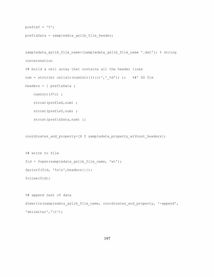
197
prefixY = 'Y';
prefixData = sampledata_gslib_file_header;
sampledata_gslib_file_name=[sampledata_gslib_file_name '.dat']; % string
concatenation
%# build a cell array that contains all the header lines
num = strtrim( cellstr(num2str((1:c)','_%d')) ); %#' SO fix
headers = [ prefixData ;
num2str(3*c) ;
strcat(prefixX,num) ;
strcat(prefixY,num) ;
strcat(prefixData,num) ];
coordinates_and_property=[X Y sampledata_property_without_headers];
%# write to file
fid = fopen(sampledata_gslib_file_name, 'wt');
fprintf(fid, '%s\n',headers{:});
fclose(fid);
%# append rest of data
dlmwrite(sampledata_gslib_file_name, coordinates_and_property, '-append',
'delimiter','\t');
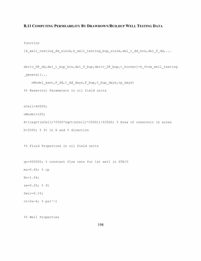
198
B.11 COMPUTING PERMEABILITY BY DRAWDOWN/BUILDUP WELL TESTING DATA
function
[k_well_testing_dd_sisim,k_well_testing_bup_sisim,del_t_dd_hrs,del_P_dd,...
deriv_DP_dd,del_t_bup_hrs,del_P_bup,deriv_DP_bup,t_horner]=k_from_well_testing
_general(...
nModel_want,P_dd,t_dd_days,P_bup,t_bup_days,tp_days)
%% Reservoir Parameters in oil field units
nCell=40000;
nModel=100;
A=((sqrt(nCell)*2500*sqrt(nCell)*2500))/43560; % Area of reservoir in acres
h=2500; % ft in X and Y direction
%% Fluid Properties in oil field units
qo=450000; % constant flow rate for 1st well in STB/D
mu=0.65; % cp
Bo=1.54;
rw=0.25; % ft
Swir=0.15;
ct=2e-6; % psi^-1
%% Well Properties
199
Nw=5; % Number of production wells
Aw=A./Nw; % Area of drainage of 1 well.
T=20; % total time in years of lease and of operating wells
xy_wells=[170,130,70,40,20;50,125,190,100,20];
xy_wells_SGEMS=[xy_wells(1,:);sqrt(nCell)-xy_wells(2,:)];
%% Computing average porosity
poro_models=gslib_file_to_mat_general(nModel,nCell,nModel_want,'poro_models_5w
ells_sisim_gslib_format');
for model_no=1:nModel_want
phi_mean(model_no)=mean(poro_models(:,model_no))/100;
end
%% Loading Drawdown test data
%# Load time steps data
% t_dd_days=load(t_dd_days);
% t_dd_days=struct2cell(t_dd_days);
% t_dd_hrs=t_dd_days{1}.*24;
%# Load BHP data
% P_dd=load(P_dd);

200
% P_dd=struct2cell(P_dd);
% P_dd=P_dd{1}';
t_dd_hrs=t_dd_days.*24;
%% Analyzing the Drawdown data numerically by diagnostic tests
%# Drawdown Pressure Difference
for model_no=1:nModel_want
for i=1:size(t_dd_hrs,1)
del_P_dd(i,model_no)=P_dd(1,model_no)-P_dd(i,model_no);
del_t_dd_hrs(i,:)=t_dd_hrs(i);
end
end
%# Drawdown Pressure Derivative
for model_no=1:nModel_want
for i=1:size(t_dd_hrs,1)-2
deriv_DP_dd(i+1,model_no)=del_t_dd_hrs(i+1)*(((((del_P_dd(i+1,model_no)-
del_P_dd(i,model_no))/(del_t_dd_hrs(i+1)-del_t_dd_hrs(i)))*(del_t_dd_hrs(i+2)-
del_t_dd_hrs(i+1)))+...
(((del_P_dd(i+2,model_no)-
del_P_dd(i+1,model_no))/(del_t_dd_hrs(i+2)-
del_t_dd_hrs(i+1)))*(del_t_dd_hrs(i+1)-del_t_dd_hrs(i))))/(del_t_dd_hrs(i+2)-
del_t_dd_hrs(i)));
201
end
end
deriv_DP_dd(size(t_dd_hrs,1),:)=0;
%% Calculating formation permeability from Drawdown
for model_no=1:nModel_want
%# Semilog Line Analysis
m_dd(model_no)=(del_P_dd(2,model_no)-
del_P_dd(1,model_no))/(del_t_dd_hrs(2)-del_t_dd_hrs(1));
C_dd(model_no)=(qo*Bo)/(24*m_dd(model_no));
CD_dd(model_no)=(C_dd(model_no)*5.615)/(2*pi*phi_mean(model_no)*ct*h*(rw^2));
poly_dd=polyfit(log(del_t_dd_hrs(size(t_dd_hrs,1)-
4:size(t_dd_hrs,1))),P_dd(size(t_dd_hrs,1)-4:size(t_dd_hrs,1),model_no),1);
m_semil_dd(model_no)=poly_dd(1);
c_1hr_dd(model_no)=poly_dd(2);
P_1hr_dd(model_no)=(m_semil_dd(model_no)*log(10)*log(1))+c_1hr_dd(model_no);
%# Computing permeability and skin factor
k_semil_dd(model_no)=-(162.6*qo*mu*Bo)/(m_semil_dd(model_no)*log(10)*h);
S_dd(model_no)=1.1513*(((P_1hr_dd(model_no)-
P_dd(1,model_no))/(m_semil_dd(model_no)*log(10)))-
log10((k_semil_dd(model_no))/(phi_mean(model_no)*mu*ct*(rw^2)))+3.23);
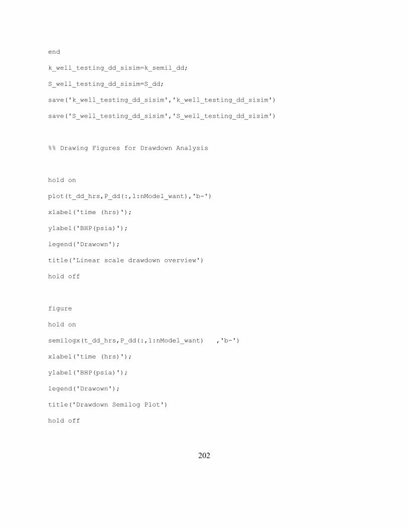
202
end
k_well_testing_dd_sisim=k_semil_dd;
S_well_testing_dd_sisim=S_dd;
save('k_well_testing_dd_sisim','k_well_testing_dd_sisim')
save('S_well_testing_dd_sisim','S_well_testing_dd_sisim')
%% Drawing Figures for Drawdown Analysis
hold on
plot(t_dd_hrs,P_dd(:,1:nModel_want),'b-')
xlabel('time (hrs)');
ylabel('BHP(psia)');
legend('Drawown');
title('Linear scale drawdown overview')
hold off
figure
hold on
semilogx(t_dd_hrs,P_dd(:,1:nModel_want) ,'b-')
xlabel('time (hrs)');
ylabel('BHP(psia)');
legend('Drawown');
title('Drawdown Semilog Plot')
hold off
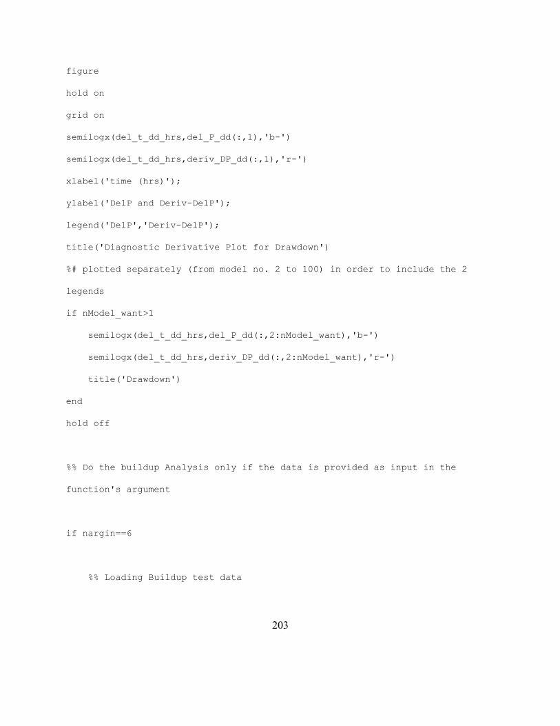
203
figure
hold on
grid on
semilogx(del_t_dd_hrs,del_P_dd(:,1),'b-')
semilogx(del_t_dd_hrs,deriv_DP_dd(:,1),'r-')
xlabel('time (hrs)');
ylabel('DelP and Deriv-DelP');
legend('DelP','Deriv-DelP');
title('Diagnostic Derivative Plot for Drawdown')
%# plotted separately (from model no. 2 to 100) in order to include the 2
legends
if nModel_want>1
semilogx(del_t_dd_hrs,del_P_dd(:,2:nModel_want),'b-')
semilogx(del_t_dd_hrs,deriv_DP_dd(:,2:nModel_want),'r-')
title('Drawdown')
end
hold off
%% Do the buildup Analysis only if the data is provided as input in the
function's argument
if nargin==6
%% Loading Buildup test data
204
%# Load time steps data
% t_bup_days=load(t_bup_days);
% t_bup_days=struct2cell(t_bup_days);
% t_bup_hrs=t_bup_days{1}.*24;
tp_hrs=tp_days*24;
%# Load BHP data
% P_bup=load(P_bup);
% P_bup=struct2cell(P_bup);
% P_bup=P_bup{1}';
t_bup_hrs=t_bup_days.*24;
%% Analyzing the Buildup data numerically by diagnostic tests
%# Buildup Pressure Difference
for model_no=1:nModel_want
for i=1:length(t_bup_hrs)
del_P_bup(i,model_no)=P_bup(i,model_no)-P_bup(1,model_no);
del_t_bup_hrs(i,:)=(t_bup_hrs(i)-tp_hrs);
t_horner(i,:)=(tp_hrs+del_t_bup_hrs(i))/del_t_bup_hrs(i);
end
end
%# Buildup Pressure Derivative
205
for model_no=1:nModel_want
for i=1:length(t_bup_hrs)-2
deriv_DP_bup(i+1,model_no)=del_t_bup_hrs(i+1)*(((((del_P_bup(i+1,model_no)-
del_P_bup(i,model_no))/(del_t_bup_hrs(i+1)-
del_t_bup_hrs(i)))*(del_t_bup_hrs(i+2)-del_t_bup_hrs(i+1)))+...
(((del_P_bup(i+2,model_no)-
del_P_bup(i+1,model_no))/(del_t_bup_hrs(i+2)-
del_t_bup_hrs(i+1)))*(del_t_bup_hrs(i+1)-
del_t_bup_hrs(i))))/(del_t_bup_hrs(i+2)-del_t_bup_hrs(i)));
deriv_P_bup(i+1,model_no)=(((((P_bup(i+1,model_no)-
P_bup(i,model_no))/(del_t_bup_hrs(i+1)-del_t_bup_hrs(i)))*(del_t_bup_hrs(i+2)-
del_t_bup_hrs(i+1)))+...
(((P_bup(i+2,model_no)-
P_bup(i+1,model_no))/(del_t_bup_hrs(i+2)-
del_t_bup_hrs(i+1)))*(del_t_bup_hrs(i+1)-
del_t_bup_hrs(i))))/(del_t_bup_hrs(i+2)-del_t_bup_hrs(i)));
end
end
deriv_DP_bup(size(t_bup_hrs,1),:)=0;
%% Calculating formation permeability from Drawdown
for model_no=1:nModel_want
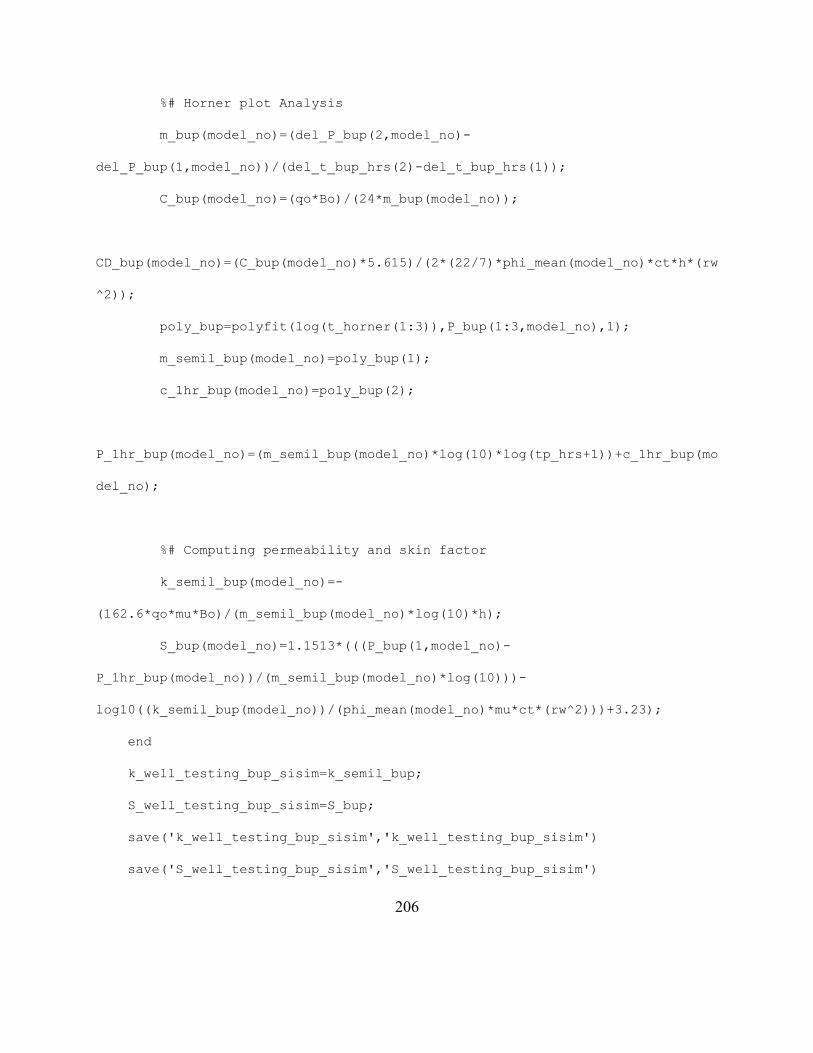
206
%# Horner plot Analysis
m_bup(model_no)=(del_P_bup(2,model_no)-
del_P_bup(1,model_no))/(del_t_bup_hrs(2)-del_t_bup_hrs(1));
C_bup(model_no)=(qo*Bo)/(24*m_bup(model_no));
CD_bup(model_no)=(C_bup(model_no)*5.615)/(2*(22/7)*phi_mean(model_no)*ct*h*(rw
^2));
poly_bup=polyfit(log(t_horner(1:3)),P_bup(1:3,model_no),1);
m_semil_bup(model_no)=poly_bup(1);
c_1hr_bup(model_no)=poly_bup(2);
P_1hr_bup(model_no)=(m_semil_bup(model_no)*log(10)*log(tp_hrs+1))+c_1hr_bup(mo
del_no);
%# Computing permeability and skin factor
k_semil_bup(model_no)=-
(162.6*qo*mu*Bo)/(m_semil_bup(model_no)*log(10)*h);
S_bup(model_no)=1.1513*(((P_bup(1,model_no)-
P_1hr_bup(model_no))/(m_semil_bup(model_no)*log(10)))-
log10((k_semil_bup(model_no))/(phi_mean(model_no)*mu*ct*(rw^2)))+3.23);
end
k_well_testing_bup_sisim=k_semil_bup;
S_well_testing_bup_sisim=S_bup;
save('k_well_testing_bup_sisim','k_well_testing_bup_sisim')
save('S_well_testing_bup_sisim','S_well_testing_bup_sisim')

207
%% Drawing Figures for Buildup Analysis
figure
hold on
plot(t_bup_hrs,P_bup(:,1:nModel_want),'b-')
xlabel('time (hrs)');
ylabel('BHP(psia)');
legend('Buildup');
title('Linear scale buildup overview')
hold off
figure
hold on
semilogx(t_horner,P_bup(:,1:nModel_want),'b-')
xlabel('Horner Time');
ylabel('BHP(psia)');
title('Buildup Horner Semilog Plot')
hold off
figure
hold on
grid on
semilogx(del_t_bup_hrs,del_P_bup(:,1),'b-')
semilogx(del_t_bup_hrs,deriv_DP_bup(:,1),'r-')

208
xlabel('time (hrs)');
ylabel('DelP and Deriv-DelP');
legend('DelP','Deriv-DelP');
title('Diagnostic Derivative Plot for Buildup')
%# plotted separately (from model no. 2 to 100) in order to include the 2
legends
if nModel_want>1
semilogx(del_t_bup_hrs,del_P_bup(:,2:nModel_want),'b-')
semilogx(del_t_bup_hrs,deriv_DP_bup(:,2:nModel_want),'r-')
title('Buildup')
end
hold off
end
209
Appendix C: MatLab Codes for Specific Cases and Chapters
This appendix presents various MatLab codes written for specific cases/chapters presented in this
thesis.
C.1 MODEL UPDATING AND VALUE OF INFORMATION (CHAPTER 3)
%% RESERVOIR PARAMETERS
nModel=100;
nModel_want=2;
nCell=2500;
A=((sqrt(nCell)*2500*sqrt(nCell)*2500))/43560; % Area of reservoir in acres
Nw=5; % Number of production wells
rw=0.25;
CA=31.62; % Shape factor for square reservoir
skin=5;
mu=0.65; % taken from CMG's Components (function of pressure)
h=500; % Paythickness in feets, and constant throughout the reservoir and in
all grids
ct=2*(10^-6);
Pi=3500; % Entered in CMG's Initial Conditions
Pwf=500;
Bo=1.54; % taken from CMG's Components (function of pressure)

210
xy_wells=[40,30,45,10,43;1,7,15,23,30];
%% ECONOMIC PARAMETERS FOR ROV and NPV ANALYSIS
%# GENERAL ECONOMIC PARAMETERS
T=20; % total time in years of lease and of operating wells
nT_BHP=24; % number of timestesps in which BHP is generated
p_oil=30; % assuming a constant oil price in dollars per barrel (bbl)
capex_5wells=600*(10^6); % investment to develop a field with 5 wells
opex=2*(10^5); % amount incurred in maintaining a well per year
r=0.12;
v_price=0.17; % volatility or standard deviation of oil prices
%# EXPLORATORY WELL SPECIFIC ECONOMIC PARAMETERS
capex_explorwell=2*(10^6); % amount incurred in drilling one EXPLORATORY well
%# SEISMIC SPECIFIC ECONOMIC PARAMETERS
capex_seismic=2*(10^6); % amount incurred in acquiring a seismic
%% COMPUTING NPV AND ROV OF THE PROJECT FOR DIFFERENT YEARS
%# Before drilling an exploratory or acquiring a seismic
[PV_5wells,NPV_5wells,ROV_5wells,q_5wells_yearly,v_5wells_yearly] =
PV_and_ROV_analysis_general(nModel,nCell,nModel_want,r,p_oil,A,Nw,rw,CA,skin,m
u,h,ct,Pi,Pwf,Bo,T,opex,capex_5wells,xy_wells,'poro_models_5wells_gslib_format

211
','perm_models_5wells_gslib_format','ReservoirModel_5wells_CMGBuilder','poro_m
odel_5wells','perm_model_5wells','Reportq_5wells');
%
[price_5wells,lattice_5wells]=BLOV_general(mean(PV_5wells(:,1)),capex_5wells,v
_5wells_yearly(2),r,T,nColumn);
%# After drilling an exploratory
[PV_explorwell,NPV_explorwell,ROV_explorwell,q_explorwell_yearly,v_explorwell_
yearly] =
PV_and_ROV_analysis_general(nModel,nCell,nModel_want,r,p_oil,A,Nw,rw,CA,skin,m
u,h,ct,Pi,Pwf,Bo,T,opex,capex_5wells+capex_explorwell,xy_wells,'poro_models_ex
plorwell_gslib_format','perm_models_explorwell_gslib_format','ReservoirModel_E
xplorWell_CMGBuilder','poro_model_explorwell','perm_model_explorwell','Reportq
_explorwell');
%
[price_explorwell,lattice_explorwell]=BLOV_general(mean(PV_explorwell(:,1)),ca
pex_5wells+capex_explorwell,v_explorwell_yearly(2),r,T,nColumn);
%# After acquiring a seismic
[PV_seismic,NPV_seismic,ROV_seismic,q_seismic_yearly,v_seismic_yearly] =
PV_and_ROV_analysis_general(nModel,nCell,nModel_want,r,p_oil,A,Nw,rw,CA,skin,m
u,h,ct,Pi,Pwf,Bo,T,opex,capex_5wells+capex_seismic,xy_wells,'poro_models_seism
ic_gslib_format','perm_models_seismic_gslib_format','ReservoirModel_Seismic_CM
GBuilder','poro_model_seismic','perm_model_seismic','Reportq_seismic');

212
%
[price_seismic,lattice_seismic]=BLOV_general(mean(PV_seismic(:,1)),capex_5well
s+capex_seismic,v_seismic_yearly(2),r,T,nColumn);
% Taking mean of all 100 models
PV_5wells_mean=mean(PV_5wells,1);
PV_explorwell_mean=mean(PV_explorwell,1);
PV_seismic_mean=mean(PV_seismic,1);
ROV_5wells_mean=mean(ROV_5wells,1);
ROV_explorwell_mean=mean(ROV_explorwell,1);
ROV_seismic_mean=mean(ROV_seismic,1);
%# VOI: ON DRILLING AN EXPLORATORY WELL AND ACQUIRING A SEISMIC RESPECTIVELY
VOI_PV_explorwell=mean(mean(PV_explorwell))-mean(mean(PV_5wells));
VOI_ROV_explorwell=mean(mean(ROV_explorwell))-mean(mean(ROV_5wells));
VOI_PV_seismic=mean(mean(PV_seismic))-mean(mean(PV_5wells));
VOI_ROV_seismic=mean(mean(ROV_seismic))-mean(mean(ROV_5wells));
%% Plotting all 100 models for PV and ROV wrt years
plot(1:T,q_5wells_yearly,'b-');
xlabel('time (yrs)');
213
ylabel('q from all 5 wells (in bbl/year)');
legend('q for 100 models with 5 production wells')
title('Prediction of Production Rate and its Uncertainty')
figure
plot(1:T,q_explorwell_yearly,'r-');
xlabel('time (yrs)');
ylabel('q from all 5 wells (in bbl/year)');
legend('q for 100 models after exploratory well')
title('Prediction of Production Rate and its Uncertainty')
figure
plot(1:T,q_seismic_yearly,'g-');
xlabel('time (yrs)');
ylabel('q from all 5 wells (in bbl/year)');
legend('q for 100 models after seismic')
title('Prediction of Production Rate and its Uncertainty')
figure
hold on
plot(1:T,q_5wells_yearly(1,:),'b-');
plot(1:T,q_seismic_yearly(1,:),'g-') % FOR SEISMIC VOI
xlabel('time (yrs)');
ylabel('q (in bbl/year)');
214
legend('q for 100 models with just 5 production wells','q for 100 models after
seismic');
%# plotted separately (from model no. 2 to 100) in order to include the two
legend colours representing before and after exploratory well
plot(1:T,q_5wells_yearly(2:nModel_want,:),'b-');
plot(1:T,q_seismic_yearly(2:nModel_want,:),'g-') % FOR SEISMIC VOI
title('Prediction of Production Rate and its
Uncertainty','Fontweight','Bold');
figure
hold on
plot(1:T,q_5wells_yearly(1,:),'b-');
plot(1:T,q_explorwell_yearly(1,:),'r-'); % FOR EXPLORATORY WELL VOI
plot(1:T,q_seismic_yearly(1,:),'g-') % FOR SEISMIC VOI
xlabel('time (yrs)');
ylabel('q (in bbl/year)');
legend('q for 100 models with just 5 production wells','q for 100 models after
exploratory well','q for 100 models after seismic');
%# plotted separately (from model no. 2 to 100) in order to include the two
legend colours representing before and after exploratory well
plot(1:T,q_5wells_yearly(2:nModel_want,:),'b-');
plot(1:T,q_explorwell_yearly(2:nModel_want,:),'r-'); % FOR EXPLORATORY WELL
VOI
plot(1:T,q_seismic_yearly(2:nModel_want,:),'g-') % FOR SEISMIC VOI
215
title('Prediction of Production Rate and its
Uncertainty','Fontweight','Bold');
figure
hold on
plot(1:T,PV_5wells(1,:),'b-');
plot(1:T,PV_explorwell(1,:),'r-'); % FOR EXPLORATORY WELL VOI
plot(1:T,PV_seismic(1,:),'g-') % FOR SEISMIC VOI
xlabel('time (yrs)');
ylabel('PV in dollars');
legend('PV for 100 models with just 5 production wells','PV for 100 models
after exploratory well','PV for 100 models after seismic');
%# plotted separately (from model no. 2 to 100) in order to include the two
legend colours representing before and after exploratory well
plot(1:T,PV_5wells(2:nModel_want,:),'b-');
plot(1:T,PV_explorwell(2:nModel_want,:),'r-'); % FOR EXPLORATORY WELL VOI
plot(1:T,PV_seismic(2:nModel_want,:),'g-') % FOR SEISMIC VOI
title('PV for exploratory well and seismic','Fontweight','Bold');
figure
hold on
plot(1:T,ROV_5wells(1,:),'b-')
plot(1:T,ROV_explorwell(1,:),'r-') % FOR EXPLORATORY WELL VOI
plot(1:T,ROV_seismic(1,:),'g-') % FOR SEISMIC VOI
xlabel('time (yrs)');
216
ylabel('ROV in dollars');
legend('ROV for 100 models with just 5 production wells','ROV for 100 models
after exploratory well','ROV for 100 models after seismic');
%# plotted separately (from model no. 2 to 100) in order to include the two
legend colours representing before and after exploratory well
plot(1:T,ROV_5wells(2:nModel_want,:),'b-')
plot(1:T,ROV_explorwell(2:nModel_want,:),'r-') % FOR EXPLORATORY WELL VOI
plot(1:T,ROV_seismic(2:nModel_want,:),'g-') % FOR SEISMIC VOI
title('ROV for exploratory well and seismic','Fontweight','Bold');
%# Plotting mean of all models for PV and ROV wrt years
figure
hold on
plot(1:T,PV_5wells_mean,'r-');
plot(1:T,PV_explorwell_mean,'g-')
plot(1:T,PV_seismic_mean,'y-')
xlabel('time (yrs)');
ylabel('PV in dollars');
legend('PV for mean of models of 5 production wells','PV for mean of models
after exploratory well','PV for mean of models after seismic');
title(['PV for mean of all ', num2str(nModel), '
models'],'Fontweight','Bold');
figure
217
hold on
plot(1:T,ROV_5wells_mean,'r-');
plot(1:T,ROV_explorwell_mean,'g-')
plot(1:T,ROV_seismic_mean,'y-')
xlabel('time (yrs)');
ylabel('ROV in dollars');
legend('ROV for mean of models of 5 production wells','ROV for mean of models
after exploratory well','ROV for mean of models after seismic');
title(['ROV for mean of all ', num2str(nModel), '
models'],'Fontweight','Bold');
C.2 ASSESSING ECONOMIC IMPLICATIONS OF RESERVOIR MODELING DECISIONS
(CHAPTER 4)
%% RESERVOIR PARAMETERS
%# All units in oil field
nCell=40000;
nModel=100;
nModel_want=100;
nModel_reference=2;
nModel_reference_want=2;
A=((sqrt(nCell)*2500*sqrt(nCell)*2500))/43560; % Area of reservoir in acres
Nw=5; % Number of production wells
218
rw=0.25;
CA=31.62; % Shape factor for square reservoir
skin=5;
mu=0.65; % taken from CMG's Components (function of pressure)
h=500; % Paythickness in feets, and constant throughout the reservoir and in
all grids
ct=2*(10^-6);
Pi=3500; % Entered in CMG's Initial Conditions
Pwf=500;
Bo=1.54; % taken from CMG's Components (function of pressure)
T=20; % total time in years of lease and of operating wells
xy_wells=[170,130,70,40,20;50,125,190,100,20];
xy_wells_SGEMS=[xy_wells(1,:);sqrt(nCell)-xy_wells(2,:)];
%% PV and ROV Analysis
%# ECONOMIC PARAMETERS FOR PV and ROV ANALYSIS
T=20; % total time in years of lease and of operating wells
p_oil=30; % assuming a constant oil price in dollars per barrel (bbl)
capex=600*(10^6); % investment to develop a field
opex=2*(10^5); % amount incurred in maintaining a well per year
r=0.12;
[PV_reference_truth,ROV_reference_truth,q_reference_truth_yearly,v_reference_t
ruth_yearly]=PV_and_ROV_analysis_general(nModel_reference,nCell,nModel_referen

219
ce_want,r,p_oil,A,Nw,rw,CA,skin,mu,h,ct,Pi,Pwf,Bo,T,opex,capex,xy_wells,'poro_
models_5wells_reference_truth_gslib_format','perm_models_5wells_reference_trut
h_gslib_format','ReservoirModel_5wells_reference_truth_CMGBuilder','poro_model
_5wells_reference_truth','perm_model_5wells_reference_truth','Reportq_5wells_r
eference_truth');
[PV_sgsim,ROV_sgsim,q_sgsim_yearly,v_sgsim_yearly]=PV_and_ROV_analysis_general
(nModel,nCell,nModel_want,r,p_oil,A,Nw,rw,CA,skin,mu,h,ct,Pi,Pwf,Bo,T,opex,cap
ex,xy_wells,'poro_models_5wells_sgsim_gslib_format','perm_models_5wells_trans_
sgsim_gslib_format','ReservoirModel_5wells_sgsim_CMGBuilder','poro_model_5well
s_sgsim','perm_model_5wells_sgsim','Reportq_5wells_sgsim');
[PV_sisim,ROV_sisim,q_sisim_yearly,v_sisim_yearly]=PV_and_ROV_analysis_general
(nModel,nCell,nModel_want,r,p_oil,A,Nw,rw,CA,skin,mu,h,ct,Pi,Pwf,Bo,T,opex,cap
ex,xy_wells,'poro_models_5wells_sisim_gslib_format','perm_models_5wells_sisim_
gslib_format','ReservoirModel_5wells_sisim_CMGBuilder','poro_model_5wells_sisi
m','perm_model_5wells_sisim','Reportq_5wells_sisim');
[PV_snesim,ROV_snesim,q_snesim_yearly,v_snesim_yearly]=PV_and_ROV_analysis_gen
eral(nModel,nCell,nModel_want,r,p_oil,A,Nw,rw,CA,skin,mu,h,ct,Pi,Pwf,Bo,T,opex
,capex,xy_wells,'poro_models_5wells_snesim_gslib_format','perm_models_5wells_s
nesim_gslib_format','ReservoirModel_5wells_snesim_CMGBuilder','poro_model_5wel
ls_snesim','perm_model_5wells_snesim','Reportq_5wells_snesim');
% Taking mean of all 100 models, of both PV and ROV
PV_reference_truth_mean=mean(PV_reference_truth,1);
PV_sgsim_mean=mean(PV_sgsim,1);
PV_sisim_mean=mean(PV_sisim,1);
220
PV_snesim_mean=mean(PV_snesim,1);
ROV_reference_truth_mean=mean(ROV_reference_truth,1);
ROV_sgsim_mean=mean(ROV_sgsim,1);
ROV_sisim_mean=mean(ROV_sisim,1);
ROV_snesim_mean=mean(ROV_snesim,1);
% Taking sum of all 20 years' production
q_sum_reference_truth_yearly=sum(q_reference_truth_yearly,2); % sum of all 20
years' production
q_sum_sgsim_yearly=sum(q_sgsim_yearly,2);
q_sum_sisim_yearly=sum(q_sisim_yearly,2);
q_sum_snesim_yearly=sum(q_snesim_yearly,2);
[n_sgsim,x_sgsim] = hist(q_sum_sgsim_yearly);
[n_sisim,x_sisim] = hist(q_sum_sisim_yearly);
[n_snesim,x_snesim] = hist(q_sum_snesim_yearly);
% Plotting distributions of q for comparison
hold on
plot(x_sgsim,n_sgsim,'rx-'); % just an example, plot the pdf with red x's and
a line, instead of bars
plot(x_sisim,n_sisim,'gx-');
plot(x_snesim,n_snesim,'kx-');
221
plot(q_sum_reference_truth_yearly(1),1,'ob')
legend('sgsim','sisim','snesim','reference-truth')
title('Comparison of distributions of production rate from different
methods','Fontweight','Bold');
%# Plotting all 100 models for PV and ROV wrt years
figure
hold on
plot(1:T,PV_reference_truth(1,:),'ob-');
plot(1:T,PV_sgsim(1,:),'r-');
plot(1:T,PV_sisim(1,:),'g-')
plot(1:T,PV_snesim(1,:),'k-')
xlabel('time (yrs)');
ylabel('PV in dollars');
legend('PV for 2 models of reference-truth','PV for 100 models of sgsim','PV
for 100 models of sisim','PV for 100 models of snesim');
%# plotted separately (from model no. 2 to 100) in order to include the 4
legends
if nModel_reference_want>=2
plot(1:T,PV_reference_truth(2:nModel_reference_want,:),'b-')
end
plot(1:T,PV_sgsim(2:nModel_want,:),'r-')
plot(1:T,PV_sisim(2:nModel_want,:),'g-')
plot(1:T,PV_snesim(2:nModel_want,:),'k-')
222
title(['PV for all', num2str(nModel), 'models'],'Fontweight','Bold');
figure
hold on
plot(1:T,ROV_reference_truth(1,:),'ob-');
plot(1:T,ROV_sgsim(1,:),'r-');
plot(1:T,ROV_sisim(1,:),'g-')
plot(1:T,ROV_snesim(1,:),'k-')
xlabel('time (yrs)');
ylabel('ROV in dollars');
legend('ROV for 2 models of reference-truth','ROV for 100 models of
sgsim','ROV for 100 models of sisim','ROV for 100 models of snesim');
%# plotted separately (from model no. 2 to 100) in order to include the 4
legends
if nModel_reference_want>=2
plot(1:T,ROV_reference_truth(2:nModel_reference_want,:),'b-')
end
plot(1:T,ROV_sgsim(2:nModel_want,:),'r-')
plot(1:T,ROV_sisim(2:nModel_want,:),'g-')
plot(1:T,ROV_snesim(2:nModel_want,:),'k-')
title(['ROV for all', num2str(nModel), 'models'],'Fontweight','Bold');
%# Plotting mean of all models for PV and ROV wrt years
figure
223
hold on
plot(1:T,PV_reference_truth_mean,'ob-');
plot(1:T,PV_sgsim_mean,'r-');
plot(1:T,PV_sisim_mean,'g-')
plot(1:T,PV_snesim_mean,'k-')
xlabel('time (yrs)');
ylabel('PV in dollars');
legend('PV for mean of models of reference-truth','PV for mean of models of
sgsim','PV for mean of models of sisim','PV for mean of models of snesim');
title(['PV for mean of all ', num2str(nModel), '
models'],'Fontweight','Bold');
figure
hold on
plot(1:T,ROV_reference_truth_mean,'ob-');
plot(1:T,ROV_sgsim_mean,'r-');
plot(1:T,ROV_sisim_mean,'g-')
plot(1:T,ROV_snesim_mean,'k-')
xlabel('time (yrs)');
ylabel('ROV in dollars');
legend('ROV for mean of models of reference-truth','ROV for mean of models of
sgsim','ROV for mean of models of sisim','ROV for mean of models of snesim');
title(['ROV for mean of all ', num2str(nModel), '
models'],'Fontweight','Bold');
224
figure
hold on
plot(1:T,v_reference_truth_yearly,'ob-');
plot(1:T,v_sgsim_yearly,'r-');
plot(1:T,v_sisim_yearly,'g-')
plot(1:T,v_snesim_yearly,'k-')
xlabel('time (yrs)');
ylabel('Project Volatility (v)');
legend('v for models of reference-truth','v for models of sgsim','v for models
of sisim','v for models of snesim');
title(['Project Volatility for all ', num2str(nModel), '
models'],'Fontweight','Bold');
C.3 ANALYZING THE PROSPECTS OF AN UNDEVELOPED FIELD (CHAPTER 6)
%% Required Parameters
%# RESERVOIR PARAMETERS
% All units in oil field
nCell=2500;
nModel=100;
nModel_want=100;
A=((sqrt(nCell)*500*sqrt(nCell)*500))/43560; % Area of reservoir in acres

225
%# ECONOMIC PARAMETERS FOR PV and ROV ANALYSIS
T=20; % total time in years of lease and of operating wells
p_oil=30; % assuming a constant oil price in dollars per barrel (bbl)
capex=600*(10^6); % investment to develop a field
opex=2*(10^5); % amount incurred in maintaining a well per year
r=0.05;
nColumn=4;
volatility=0.20;
%% NPV and BLOV Analysis for 5 Scenarios
%# NPV estimation by using 'NPV_reserve_by_STOOIP.m'
[NPV_reference,P10_reference,P25_reference,P50_reference,P75_reference,...
P90_reference,vol_reserve_reference]=NPV_reserve_by_STOOIP_general(nModel,nMod
el_want,nCell,'poro_models_5wells_gslib_format');
[NPV_seismic,P10_seismic,P25_seismic,P50_seismic,P75_seismic,P90_seismic,...
vol_reserve_seismic]=NPV_reserve_by_STOOIP_general(nModel,nModel_want,nCell,'p
oro_models_seismic_gslib_format');
percentiles_reference=[P90_reference,P75_reference,P50_reference,P25_reference
,P10_reference];
netP_reference=sum([0.90,0.75,0.50,0.25,0.10].*percentiles_reference);

226
percentiles_seismic=[P90_seismic,P75_seismic,P50_seismic,P25_seismic,P10_seism
ic];
netP_seismic=sum([0.90,0.75,0.50,0.25,0.10].*percentiles_seismic);
%# BLOV analysis by using 'BLOV_general.m'
[price_reference,lattice_reference]=BLOV_general(netP_reference,capex,volatili
ty,r,T,nColumn,'Option NPV Forecast by using reference only','Underlying
lattice by using reference only');
[price_reference90,lattice_reference90]=BLOV_general(percentiles_reference(1),
capex,volatility,r,T,nColumn);
[price_reference75,lattice_reference75]=BLOV_general(percentiles_reference(2),
capex,volatility,r,T,nColumn);
[price_reference50,lattice_reference50]=BLOV_general(percentiles_reference(3),
capex,volatility,r,T,nColumn);
[price_reference25,lattice_reference25]=BLOV_general(percentiles_reference(4),
capex,volatility,r,T,nColumn);
[price_reference10,lattice_reference10]=BLOV_general(percentiles_reference(5),
capex,volatility,r,T,nColumn);
[price_seismic,lattice_seismic]=BLOV_general(netP_seismic,capex,volatility,r,T
,nColumn,'Option NPV Forecast by using reference and seismic','Underlying
lattice by using reference and seismic');
[price_seismic90,lattice_seismic90]=BLOV_general(percentiles_seismic(1),capex,
volatility,r,T,nColumn);
227
[price_seismic75,lattice_seismic75]=BLOV_general(percentiles_seismic(2),capex,
volatility,r,T,nColumn);
[price_seismic50,lattice_seismic50]=BLOV_general(percentiles_seismic(3),capex,
volatility,r,T,nColumn);
[price_seismic25,lattice_seismic25]=BLOV_general(percentiles_seismic(4),capex,
volatility,r,T,nColumn);
[price_seismic10,lattice_seismic10]=BLOV_general(percentiles_seismic(5),capex,
volatility,r,T,nColumn);
%% Figures
%# Plotting Histograms
figure
hist(NPV_reference)
xlabel('NPV (in $)')
ylabel('Frequency')
title(['Distribution of NPV by using reference only ', num2str(nModel), '
models'],'Fontweight','Bold');
figure
hist(NPV_seismic)
xlabel('NPV (in $)')
ylabel('Frequency')
title(['Distribution of NPV by using reference and seismic ', num2str(nModel),
' models'],'Fontweight','Bold');
228
%# Plotting P10, P25, P50, P75, and P90 for NPV
figure
x = 1:5;
y = [P10_reference,P25_reference,P50_reference,P75_reference,P90_reference];
plot(x, y, '-ob')
set(gca, 'XTick',1:5, 'XTickLabel',{'P10' 'P25' 'P50' 'P75' 'P90'})
title('P-values by using reference only','Fontweight','Bold')
ylabel('NPV($)')
figure
x = 1:5;
y = [P10_seismic,P25_seismic,P50_seismic,P75_seismic,P90_seismic];
plot(x, y, '-ob')
set(gca, 'XTick',1:5, 'XTickLabel',{'P10' 'P25' 'P50' 'P75' 'P90'})
title('P-values using reference and seismic','Fontweight','Bold')
ylabel('NPV($)')
%# Plotting option values corresponding to P10, P25, P50, P75, and P90
figure
hold on
x = 1:5;
y_reference =
[price_reference10,price_reference25,price_reference50,price_reference75,price
_reference90];
229
y_seismic =
[price_seismic10,price_seismic25,price_seismic50,price_seismic75,price_seismic
90];
plot(x, y_reference, '-ob')
plot(x, y_seismic, '-or')
set(gca, 'XTick',1:5, 'XTickLabel',{'P10' 'P25' 'P50' 'P75' 'P90'})
title('Option values corresponding to each P-value','Fontweight','Bold')
ylabel('Option Value ($)')
legend('by using reference only','by using reference and seismic')
hold off
C.4 ANALYZING RESERVOIR PERFORMANCE BY MODEL SELECTION (CHAPTER 7)
%% Required Parameters
%# RESERVOIR PARAMETERS
% All units in oil field
nCell=40000;
nModel=100;
nModel_want=100;
A=((sqrt(nCell)*500*sqrt(nCell)*500))/43560; % Area of reservoir in acres
Nw=5; % Number of production wells
rw=0.25;
CA=31.62; % Shape factor for square reservoir

230
skin=5;
mu=0.65; % taken from CMG's Components (function of pressure)
h=500; % Paythickness in feets, and constant throughout the reservoir and in
all grids
ct=2*(10^-6);
Pi=3500; % Entered in CMG's Initial Conditions
Pwf=500;
Bo=1.54; % taken from CMG's Components (function of pressure)
xy_wells=[40,30,45,10,43;1,7,15,23,30];
%# ECONOMIC PARAMETERS FOR PV and ROV ANALYSIS
T=20; % total time in years of lease and of operating wells
p_oil=30; % assuming a constant oil price in dollars per barrel (bbl)
capex=6000*(10^6); % investment to develop a field
opex=2*(10^5); % amount incurred in maintaining a well per year
r=0.05;
nColumn=4;
volatility=0.20;
%% Choosing the common models from model selection by two well test history
data
%# reading selected models obtained using two well test history data
model_list1=importdata('model_list_by_well_1_history.txt',' ',1);
model_list1=struct2cell(model_list1);
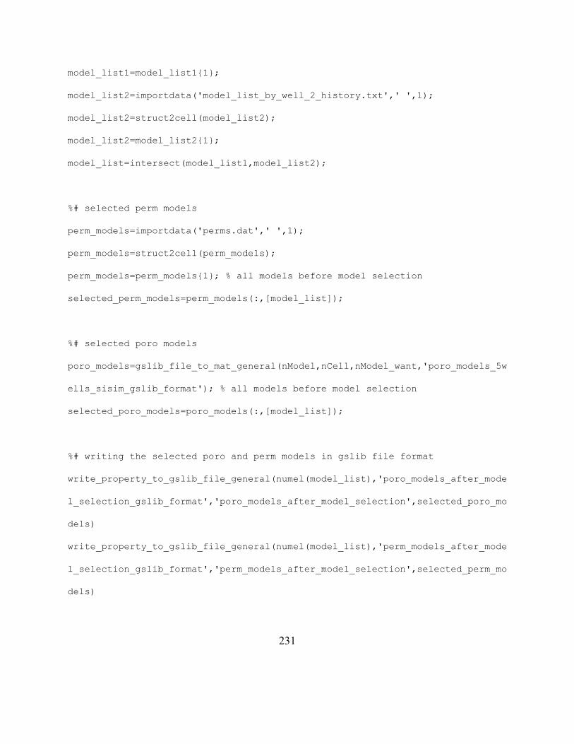
231
model_list1=model_list1{1};
model_list2=importdata('model_list_by_well_2_history.txt',' ',1);
model_list2=struct2cell(model_list2);
model_list2=model_list2{1};
model_list=intersect(model_list1,model_list2);
%# selected perm models
perm_models=importdata('perms.dat',' ',1);
perm_models=struct2cell(perm_models);
perm_models=perm_models{1}; % all models before model selection
selected_perm_models=perm_models(:,[model_list]);
%# selected poro models
poro_models=gslib_file_to_mat_general(nModel,nCell,nModel_want,'poro_models_5w
ells_sisim_gslib_format'); % all models before model selection
selected_poro_models=poro_models(:,[model_list]);
%# writing the selected poro and perm models in gslib file format
write_property_to_gslib_file_general(numel(model_list),'poro_models_after_mode
l_selection_gslib_format','poro_models_after_model_selection',selected_poro_mo
dels)
write_property_to_gslib_file_general(numel(model_list),'perm_models_after_mode
l_selection_gslib_format','perm_models_after_model_selection',selected_perm_mo
dels)

232
%% NPV Analysis by Tank Method and BLOV: Before Model Selection
%# NPV estimation by using 'PV_and_ROV_analysis_general.m'
[PV_before_model_selection,NPV_before_model_selection,ROV_before_model_selecti
on,q_before_model_selection,volatility_LR_sum_PV,volatility_LR_sum_NPV] =
PV_and_ROV_analysis_general(nModel,nCell,nModel_want,r,p_oil,A,Nw,rw,CA,skin,m
u,h,ct,Pi,Pwf,Bo,T,opex,capex,xy_wells,'poro_models_5wells_sisim_gslib_format'
,'perm_models_5wells_sisim_gslib_format');
percentiles_before_model_selection=prctile(NPV_before_model_selection(:,T),[10
,25,50,75,90]);
P90_before_model_selection=percentiles_before_model_selection(1);
P75_before_model_selection=percentiles_before_model_selection(2);
P50_before_model_selection=percentiles_before_model_selection(3);
P25_before_model_selection=percentiles_before_model_selection(4);
P10_before_model_selection=percentiles_before_model_selection(5);
netP_before_model_selection=sum([0.90,0.75,0.50,0.25,0.10].*percentiles_before
_model_selection);
%# BLOV analysis by using 'BLOV_general.m'
[price_before_model_selection,lattice_before_model_selection]=BLOV_general(net
P_before_model_selection,capex,volatility_LR_sum_PV(2),r,T,nColumn,'Option
lattice before the model selection','Underlying lattice before the model
selection');

233
[price_before_model_selection90,lattice_before_model_selection90]=BLOV_general
(percentiles_before_model_selection(1),capex,volatility_LR_sum_PV(2),r,T,nColu
mn);
[price_before_model_selection75,lattice_before_model_selection75]=BLOV_general
(percentiles_before_model_selection(2),capex,volatility_LR_sum_PV(2),r,T,nColu
mn);
[price_before_model_selection50,lattice_before_model_selection50]=BLOV_general
(percentiles_before_model_selection(3),capex,volatility_LR_sum_PV(2),r,T,nColu
mn);
[price_before_model_selection25,lattice_before_model_selection25]=BLOV_general
(percentiles_before_model_selection(4),capex,volatility_LR_sum_PV(2),r,T,nColu
mn);
[price_before_model_selection10,lattice_before_model_selection10]=BLOV_general
(percentiles_before_model_selection(5),capex,volatility_LR_sum_PV(2),r,T,nColu
mn);
%% NPV Analysis by Tank Method and BLOV: After Model Selection
%# NPV estimation by using 'PV_and_ROV_analysis_general.m'
[PV_after_model_selection,NPV_after_model_selection,ROV_after_model_selection,
q_after_model_selection,volatility_LR_sum_PV,volatility_LR_sum_NPV] =
PV_and_ROV_analysis_general(numel(model_list),nCell,numel(model_list),r,p_oil,
A,Nw,rw,CA,skin,mu,h,ct,Pi,Pwf,Bo,T,opex,capex,xy_wells,'poro_models_after_mod
el_selection_gslib_format','perm_models_after_model_selection_gslib_format');
234
percentiles_after_model_selection=prctile(NPV_after_model_selection(:,T),[10,2
5,50,75,90]);
P90_after_model_selection=percentiles_after_model_selection(1);
P75_after_model_selection=percentiles_after_model_selection(2);
P50_after_model_selection=percentiles_after_model_selection(3);
P25_after_model_selection=percentiles_after_model_selection(4);
P10_after_model_selection=percentiles_after_model_selection(5);
netP_after_model_selection=sum([0.90,0.75,0.50,0.25,0.10].*percentiles_after_m
odel_selection);
%# BLOV analysis by using 'BLOV_general.m'
[price_after_model_selection,lattice_after_model_selection]=BLOV_general(netP_
after_model_selection,capex,volatility_LR_sum_PV(2),r,T,nColumn,'Option
lattice after the model selection','Underlying lattice after the model
selection');
[price_after_model_selection90,lattice_after_model_selection90]=BLOV_general(p
ercentiles_after_model_selection(1),capex,volatility_LR_sum_PV(2),r,T,nColumn)
;
[price_after_model_selection75,lattice_after_model_selection75]=BLOV_general(p
ercentiles_after_model_selection(2),capex,volatility_LR_sum_PV(2),r,T,nColumn)
;
[price_after_model_selection50,lattice_after_model_selection50]=BLOV_general(p
ercentiles_after_model_selection(3),capex,volatility_LR_sum_PV(2),r,T,nColumn)
;
235
[price_after_model_selection25,lattice_after_model_selection25]=BLOV_general(p
ercentiles_after_model_selection(4),capex,volatility_LR_sum_PV(2),r,T,nColumn)
;
[price_after_model_selection10,lattice_after_model_selection10]=BLOV_general(p
ercentiles_after_model_selection(5),capex,volatility_LR_sum_PV(2),r,T,nColumn)
;
%% Figures
%# Plotting Histograms
figure
hist(NPV_before_model_selection(:,T))
xlabel('NPV (in $)')
ylabel('Frequency')
title(['Distribution of NPV for ', num2str(nModel), ' models before model
selection'],'Fontweight','Bold');
figure
hist(NPV_after_model_selection(:,T))
xlabel('NPV (in $)')
ylabel('Frequency')
title(['Distribution of NPV for ', num2str(numel(model_list)), ' models after
model selection'],'Fontweight','Bold');
%# Plotting P10, P25, P50, P75 and P90
236
figure
x = 1:5;
y =
[P10_before_model_selection,P25_before_model_selection,P50_before_model_select
ion,P75_before_model_selection,P90_before_model_selection];
plot(x, y, '-ob')
set(gca, 'XTick',1:5, 'XTickLabel',{'P10' 'P25' 'P50' 'P75' 'P90'})
title('P-values for NPV before model selection','Fontweight','Bold')
ylabel('NPV($)')
figure
x = 1:5;
y =
[P10_after_model_selection,P25_after_model_selection,P50_after_model_selection
,P75_after_model_selection,P90_after_model_selection];
plot(x, y, '-ob')
set(gca, 'XTick',1:5, 'XTickLabel',{'P10' 'P25' 'P50' 'P75' 'P90'})
title('P-values for NPV after model selection','Fontweight','Bold')
ylabel('NPV($)')
%# Plotting option values corresponding to P10, P25, P50, P75, and P90
figure
hold on
x = 1:5;
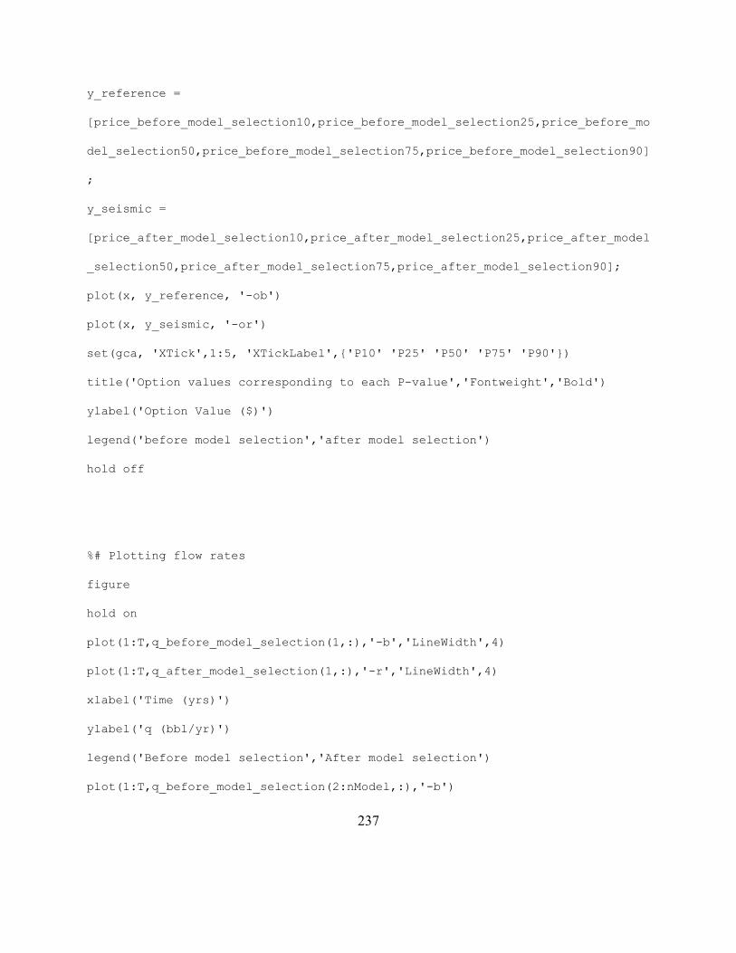
237
y_reference =
[price_before_model_selection10,price_before_model_selection25,price_before_mo
del_selection50,price_before_model_selection75,price_before_model_selection90]
;
y_seismic =
[price_after_model_selection10,price_after_model_selection25,price_after_model
_selection50,price_after_model_selection75,price_after_model_selection90];
plot(x, y_reference, '-ob')
plot(x, y_seismic, '-or')
set(gca, 'XTick',1:5, 'XTickLabel',{'P10' 'P25' 'P50' 'P75' 'P90'})
title('Option values corresponding to each P-value','Fontweight','Bold')
ylabel('Option Value ($)')
legend('before model selection','after model selection')
hold off
%# Plotting flow rates
figure
hold on
plot(1:T,q_before_model_selection(1,:),'-b','LineWidth',4)
plot(1:T,q_after_model_selection(1,:),'-r','LineWidth',4)
xlabel('Time (yrs)')
ylabel('q (bbl/yr)')
legend('Before model selection','After model selection')
plot(1:T,q_before_model_selection(2:nModel,:),'-b')

238
plot(1:T,q_after_model_selection(2:numel(model_list),:),'-r')
title('Uncertainty in oil flow rate from 5 wells','Fontweight','Bold')

239
Bibliography
Arps, J.J., 1945. Analysis of Decline Curves. Transactions of the American Institute of Mining,
Metallurgical and Petroleum Engineers, 160, pp.228–247.
Bailey, W., Bhandari, A., Faiz, S., Srinivasan, S., Weeds, H., 2003. Unlocking the Value of Real
Options (Oilfield Review), Schlumberger. , 15(4).
Bhowmik, S., Srinivasan, S. & Bryant, S., 2010. Predicting the Migration of CO2 Plume Using
Injection Data and a Distance-Metric Approach to Reservoir-Model Selection. In
Proceedings of SPE International Conference on CO2 Capture, Storage, and Utilization.
SPE International Conference on CO2 Capture, Storage, and Utilization.
CMG-IMEX, 2009. IMEX - User’s Guide: Advanced IMplicit-EXplicit Black Oil Simulator
2009th ed., Calgary, Alberta: Computer Modelling Group Ltd.
Copeland, T.E. & Antikarov, V., 2001. Real options: a practitioner’s guide, Texere.
Cox, J.C., Ross, S.A. & Rubinstein, M., 1979. Option pricing: A simplified approach. Journal of
Financial Economics, 7(3), pp.229–263.
Coy, P., 1999. Exploiting Uncertainty. Business Week (US edition), (no. 3632), pp.118–124.
DePamphilis, D.M., 2009. Mergers, Acquisitions, and Other Restructuring Activities: An
Integrated Approach to Process, Tools, Cases, and Solutions, Academic Press.
Deutsch, C.V. & Journel, A.G., 1997. GSLIB: Geostatistical Software Library and User’s Guide
2nd ed., Oxford University Press, USA.
240
Dias, M.A., 2004. Monte Carlo Simulation of Stochastic Processes. http://www.puc-
rio.br/marco.ind/sim_stoc_proc.html#mc-mrd.
Dixit, A. & Pindyck, R., 1995. Options Approach to Capital Investment - Harvard Business
Review. Harvard Business Review, p.13.
Energy Information Administration - EIA, 2008. Defining the Limits of Oil Production. In
International Energy Outlook 2008. U.S. Department of Energy.
Eskandari, K. & Srinivasan, S., 2010. Reservoir Modelling of Complex Geological Systems--A
Multiple-Point Perspective. Journal of Canadian Petroleum Technology, 49(8).
Johnson, N.W., 2010. Response to Peter Monkhouse. Economic Analysis and Policy (EAP),
40(1), pp.112–123.
Lin, J., 2008. Exploring flexible strategies in engineering systems using screening models :
applications to offshore petroleum projects. PhD Dissertation. Massachusetts:
Massachusetts Institute of Technology.
Mun, J., 2002. Real options analysis: tools and techniques for valuing strategic investments and
decisions, John Wiley and Sons.
Ornstein, L.S. & Uhlenbeck, G.E., 1930. On the Theory of the Brownian Motion. Physical
Review, 36(5), p.823.
Remy, N., Boucher, A. & Wu, J., 2009. Applied Geostatistics with SGeMS: A User’s Guide 1
Har/Cdr., Cambridge University Press.
Samuelson, P.A., 1965. Proof that properly anticipated prices fluctuate randomly. Industrial
Management Review.
241
Strabelle, S., 2000. Sequential simulation drawing structures from training images. PhD Thesis.
Stanford University. Available at: http://gcmd.nasa.gov/records/SGEMS.html
Ugur, O., 2008. Introduction to Computational Finance, Imperial College Press.
Walsh, M.P. & Lake, L.W., 2003. A generalized approach to primary hydrocarbon recovery,
Elsevier.
Xu, W., Tran, T., Srivastava, R. M., Journel, A. G., 1992. Integrating Seismic Data in Reservoir
Modeling: The Collocated Cokriging Alternative. In Society of Petroleum Engineers.
Young, E.& & Wiley, J., 2011. International GAAP 2012: Generally Accepted Accounting
Practice Under International Financial Reporting Standards, John Wiley & Sons.
Zhu & Journel, 1993. Formatting and integrating soft data: Stochastic imaging via the Markov-
Bayes algorithm. Soares, A. (Ed.), Geostatistics Troia’92, Kluwer Academic Publishers,
Dordrecht, Holland, pp.1–12.