Click to Start Higher Maths Unit 3 Chapter 3 Logarithms Experiment & Theory.
date post
18-Dec-2015Category
view
221download
1
Copyright © 2006 Pearson Addison-Wesley. All rights reserved.
Lecture 6:Interpreting Regression Results
Logarithms (Chapter 4.5)
Standard Errors(Chapter 5)

Copyright © 2006 Pearson Addison-Wesley. All rights reserved. 6-2
Agenda for Today
• Review
• Logarithms in Econometrics (Chapter 4.5)
• Residuals (Chapter 5.1)
• Estimating an Estimator’s Variance (Chapter 5.2)
• Confidence Intervals (Chapter 5.4)
Copyright © 2006 Pearson Addison-Wesley. All rights reserved. 6-3
Review
• As a starting place for analysis, we need to write down all our assumptions about the way the underlying process works, and about how that process led to our data.
• These assumptions are called the “Data Generating Process.”
• Then we can derive estimators that have good properties for the Data Generating Process we have assumed.
Copyright © 2006 Pearson Addison-Wesley. All rights reserved. 6-4
Review: The Gauss–Markov DGP
• Y = X +• E(i ) = 0
• Var(i ) = 2
• Cov(i ,j ) = 0, for i ≠ j
• X ’s fixed across samples (so we can treat them like constants).
• We want to estimate
Copyright © 2006 Pearson Addison-Wesley. All rights reserved. 6-5
Review
2
1
1
1
( ) 0
( ) ( , ) 0,
ˆ
ˆ( )
1.
i i i i
i i j
n
i ii
n
i ii
n
i ii
Y X E
Var Cov i j
X
wY
E w X
w X
for
's fixed across samples
A linear estimator is unbiased if

Copyright © 2006 Pearson Addison-Wesley. All rights reserved. 6-6
Review (cont.)
A linear estimator is unbiased if wiX
ii1
n
1.
Many linear estimators will be unbiased.
How do I pick the "best" linear
unbiased estimator (BLUE)?
Copyright © 2006 Pearson Addison-Wesley. All rights reserved. 6-7
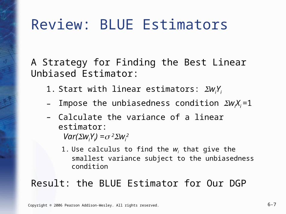
Review: BLUE Estimators
A Strategy for Finding the Best Linear Unbiased Estimator:
1. Start with linear estimators: wiYi
– Impose the unbiasedness condition wiXi =1
– Calculate the variance of a linear estimator: Var(wiYi) =2wi
2
1. Use calculus to find the wi that give the smallest variance subject to the unbiasedness condition
Result: the BLUE Estimator for Our DGP
Copyright © 2006 Pearson Addison-Wesley. All rights reserved. 6-8
Review: BLUE Estimators (cont.)
• Ordinary Least Squares (OLS) is BLUE for our Gauss–Markov DGP.
• This result is called the “Gauss–Markov Theorem.”
Copyright © 2006 Pearson Addison-Wesley. All rights reserved. 6-9
Review: BLUE Estimators (cont.)
• OLS is a very good strategy for the Gauss–Markov DGP.
• OLS is unbiased: our guesses are right on average.
• OLS is efficient: it has a small variance (or at least the smallest possible variance for unbiased linear estimators).
Copyright © 2006 Pearson Addison-Wesley. All rights reserved. 6-10
Review: BLUE Estimators (cont.)
• Our guesses will tend to be close to right (or at least as close to right as we can get).
• Warning: the minimum variance could still be pretty large!
Copyright © 2006 Pearson Addison-Wesley. All rights reserved. 6-11
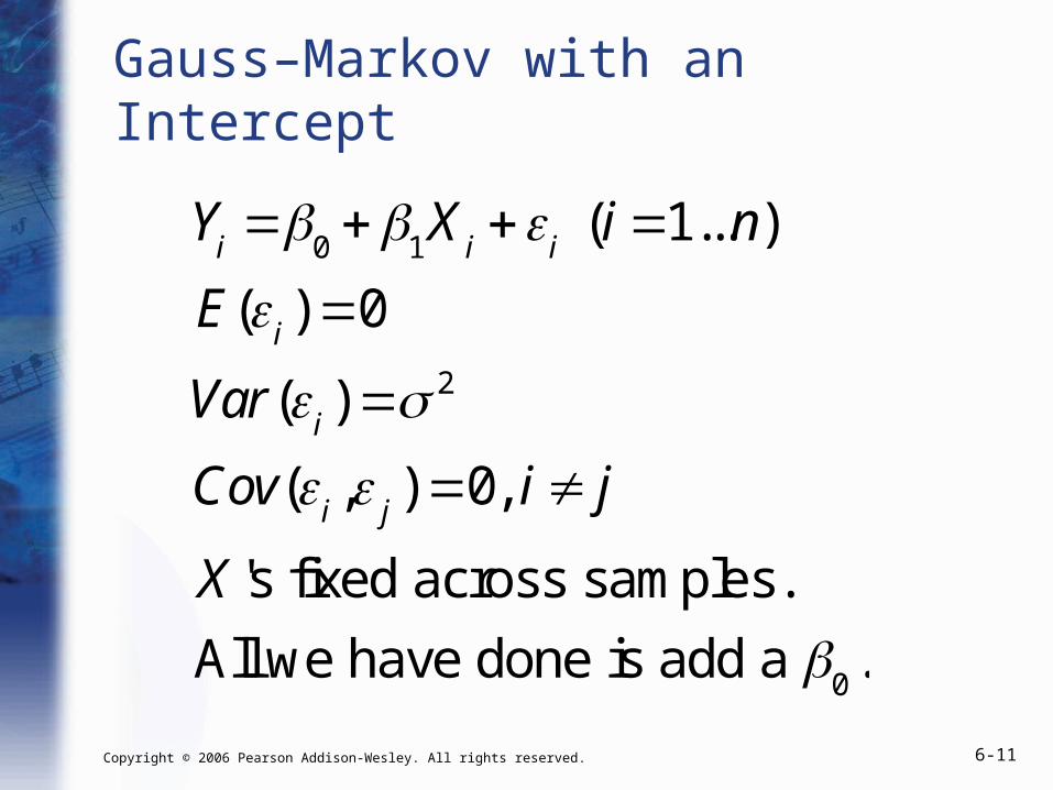
Gauss–Markov with an Intercept
Yi
0
1X
i
i (i 1...n)
E(i) 0
Var(i) 2
Cov(i,
j) 0, i j
X 's fixed across samples.
All we have done is add a 0.
Copyright © 2006 Pearson Addison-Wesley. All rights reserved. 6-12
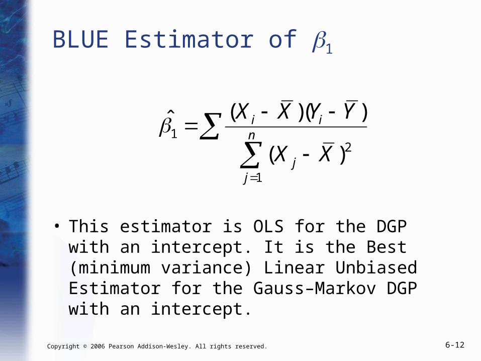
BLUE Estimator of 1
12
1
( )( )ˆ ( )
i in
jj
X X Y Y
X X
• This estimator is OLS for the DGP with an intercept. It is the Best (minimum variance) Linear Unbiased Estimator for the Gauss–Markov DGP with an intercept.

Copyright © 2006 Pearson Addison-Wesley. All rights reserved. 6-13
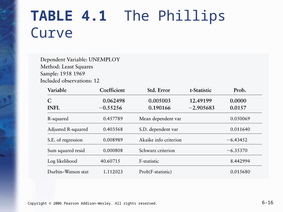
Example: The Phillips Curve
• The US data from 1958–1969 suggest a trade-off between inflation and unemployment.
0
1
ˆ 0.06
ˆ 0.55
Unemploymentt 0.06 - 0.55·Inflationt
Copyright © 2006 Pearson Addison-Wesley. All rights reserved. 6-14
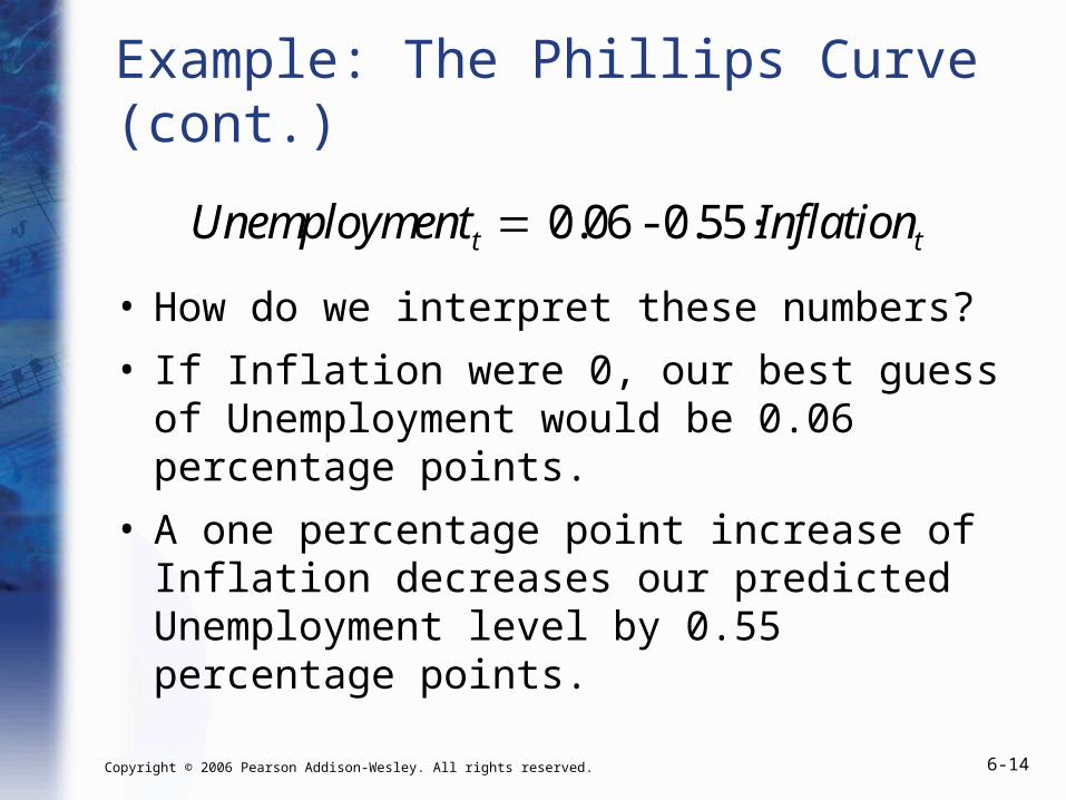
Example: The Phillips Curve (cont.)
• How do we interpret these numbers?
• If Inflation were 0, our best guess of Unemployment would be 0.06 percentage points.
• A one percentage point increase of Inflation decreases our predicted Unemployment level by 0.55 percentage points.
Unemploymentt 0.06 - 0.55·Inflationt

Copyright © 2006 Pearson Addison-Wesley. All rights reserved. 6-15
Figure 4.2 U.S. Unemployment and Inflation, 1958–1969
Copyright © 2006 Pearson Addison-Wesley. All rights reserved. 6-16
TABLE 4.1 The Phillips Curve

Copyright © 2006 Pearson Addison-Wesley. All rights reserved. 6-17
Example: Phillips Curve
• A straight line seems not quite to capture the data.
• A curve would fit better.
• Can we use linear estimators to fit non-linear relationships?
Copyright © 2006 Pearson Addison-Wesley. All rights reserved. 6-18
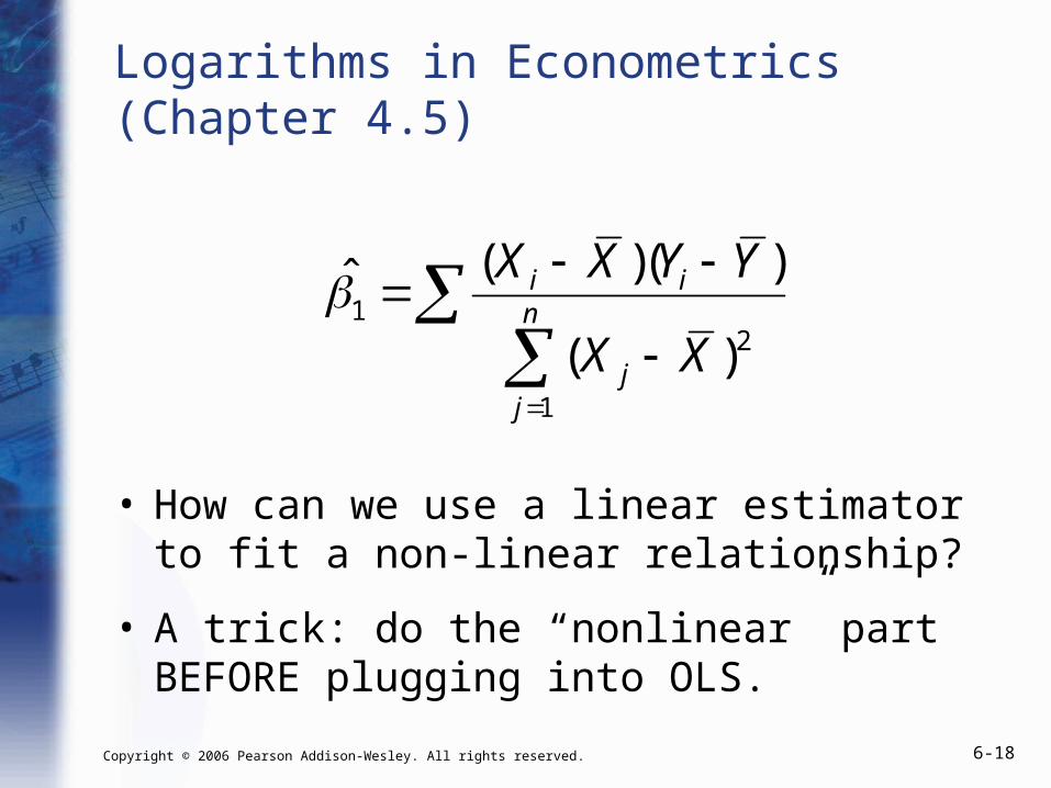
Logarithms in Econometrics (Chapter 4.5)
12
1
( )( )ˆ
( )
i in
jj
X X Y Y
X X
• How can we use a linear estimator to fit a non-linear relationship?
• A trick: do the “nonlinear” part BEFORE plugging into OLS.
Copyright © 2006 Pearson Addison-Wesley. All rights reserved. 6-19
Logarithms in Econometrics (cont.)
12
1
( )( )ˆ ( )
i in
jj
X X Y Y
X X
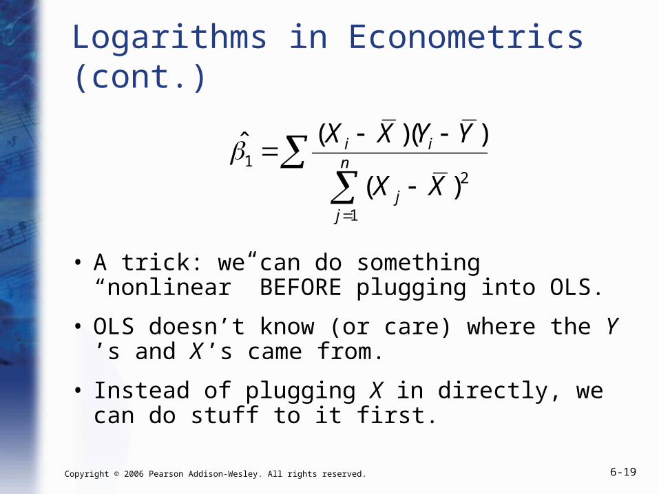
• A trick: we can do something “nonlinear” BEFORE plugging into OLS.
• OLS doesn’t know (or care) where the Y ’s and X ’s came from.
• Instead of plugging X in directly, we can do stuff to it first.
Copyright © 2006 Pearson Addison-Wesley. All rights reserved. 6-20
Logarithms in Econometrics (cont.)
• We can do “stuff” to X and Y before we plug them into our OLS formula.
• If we do something nonlinear to Y and/or X, then our linear regression of new-nonlinear-Y on new-nonlinear-X will plot a nonlinear relationship between Y and X.
• What can we do to X and Y to fit a curve?

Copyright © 2006 Pearson Addison-Wesley. All rights reserved. 6-21
Logarithms in Econometrics (cont.)
• LOGARITHMS!!!!!!!!!!!!
• Regress
• How do we interpret our estimated coefficients?
• Our fitted value for 1 no longer tells us the effect of a 1-unit change in X on Y. It tells us the effect of a 1-unit change in log(X) on log(Y).
log(Y ) 0 1·log(X)

Copyright © 2006 Pearson Addison-Wesley. All rights reserved. 6-22
Logarithms in Econometrics (cont.)
• Regress
• Our fitted value for 1 no longer tells us the effect of a 1-unit change in X on Y. It tells us the effect of a 1-unit change in log(X) on log(Y).
• Unit changes in log-X translate into PERCENTAGE changes in X.
log(Y ) 0 1·log(X)

Copyright © 2006 Pearson Addison-Wesley. All rights reserved. 6-23
• Regress
• Unit changes in log(X) translate into PERCENTAGE changes in X.
• Our estimate tells us the percentage change in Y we predict from a 1-percent change in X.
1
Logarithms in Econometrics (cont.)
log(Y ) 0 1·log(X)

Copyright © 2006 Pearson Addison-Wesley. All rights reserved. 6-24
• The percentage change in Y from a 1-percent change in X has a special name in economics—elasticity!
• Taking logs of both Y and X lets us estimate elasticities!
Logarithms in Econometrics (cont.)
log(Y ) 0 1·log(X)
Copyright © 2006 Pearson Addison-Wesley. All rights reserved. 6-25
Example: The Phillips Curve
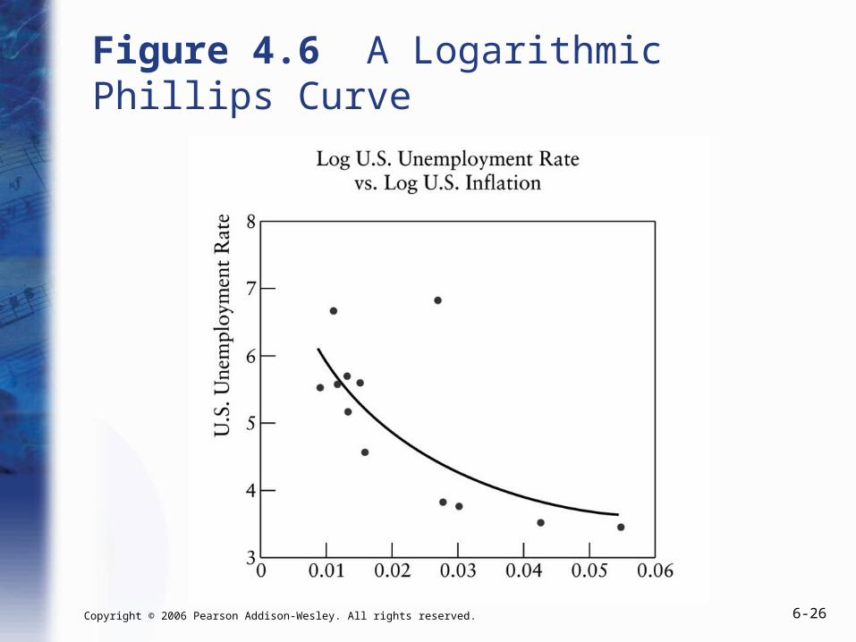
• If we log both Unemployment and Inflation, then we can predict the percentage change in unemployment resulting from a one percent change in inflation.
• Percentage changes are nonlinear. Changing inflation from 0.01 to 0.02 is a 100% increase. Changing inflation from 0.02 to 0.03 is only a 50% increase.
Copyright © 2006 Pearson Addison-Wesley. All rights reserved. 6-26
Figure 4.6 A Logarithmic Phillips Curve

Copyright © 2006 Pearson Addison-Wesley. All rights reserved. 6-27
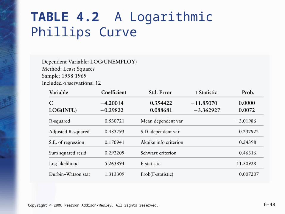
TABLE 4.2 A Logarithmic Phillips Curve
Copyright © 2006 Pearson Addison-Wesley. All rights reserved. 6-28
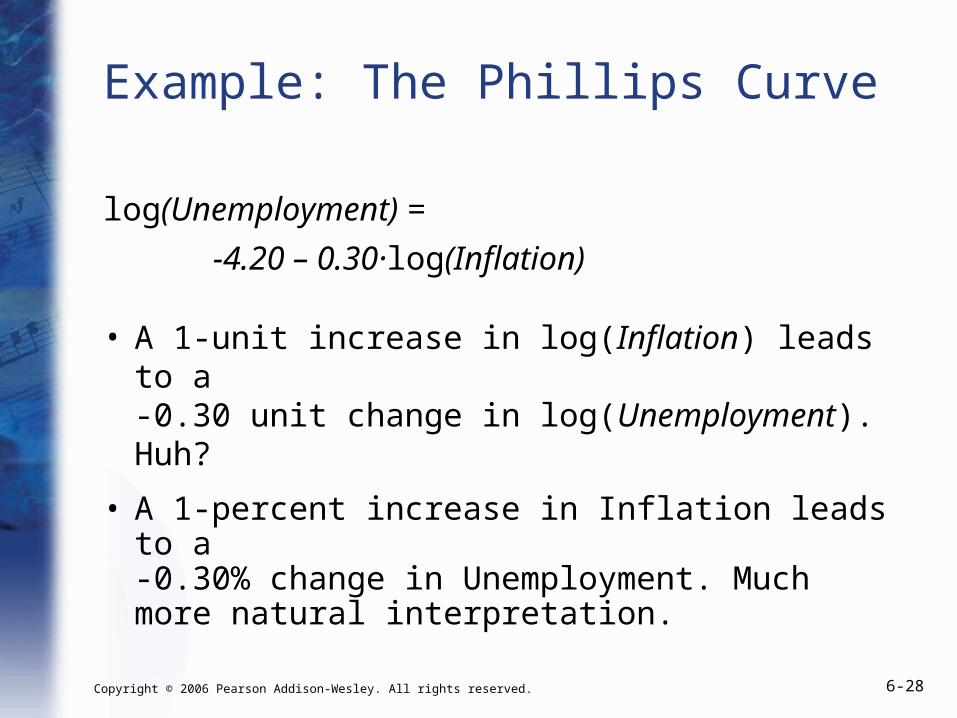
Example: The Phillips Curve
log(Unemployment) =
-4.20 – 0.30·log(Inflation)
• A 1-unit increase in log(Inflation) leads to a -0.30 unit change in log(Unemployment). Huh?
• A 1-percent increase in Inflation leads to a -0.30% change in Unemployment. Much more natural interpretation.
Copyright © 2006 Pearson Addison-Wesley. All rights reserved. 6-29
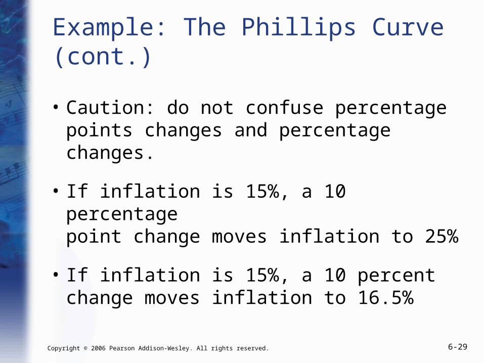
Example: The Phillips Curve (cont.)
• Caution: do not confuse percentage points changes and percentage changes.
• If inflation is 15%, a 10 percentage point change moves inflation to 25%
• If inflation is 15%, a 10 percent change moves inflation to 16.5%
Copyright © 2006 Pearson Addison-Wesley. All rights reserved. 6-30
0 1i i iY X
Residuals (Chapter 5.1)
• So far, we have learned how to predict lines with an intercept and a single explanator.
• We have focused on making our “best guess” estimates of the intercept and slope of the line.

Copyright © 2006 Pearson Addison-Wesley. All rights reserved. 6-31
Residuals (cont.)
• Once we have run our regression, we can make our best guess about what the Y value would be for an observation with some specified value of X.
• Our best guesses about the Y values are called “predictions.”
• If we have an unbiased estimator, we expect our predictions to be right on average.
Copyright © 2006 Pearson Addison-Wesley. All rights reserved. 6-32
Residuals (cont.)
• Our best guesses about the Y values are called “predictions.”
• If we have an unbiased estimator, we expect our predictions to be right on average.
• For any given observation, our predictions will be WRONG.

Copyright © 2006 Pearson Addison-Wesley. All rights reserved. 6-33
Residuals (cont.)
• Our “best guess” of Yi (conditioned on knowing Xi) is:
• On average, we expect a one-unit increase in X to increase Y by units.
0 1ˆ ˆ
i iY X
1
Copyright © 2006 Pearson Addison-Wesley. All rights reserved. 6-34
Residuals (cont.)
• Our “best guess” of Yi (conditioned on knowing Xi) is:
• An individual observation, though, is subject to various factors that are outside our model, such as omitted variables or simple chance.
0 1ˆ ˆ
i iY X
Copyright © 2006 Pearson Addison-Wesley. All rights reserved. 6-35
0 1ˆ ˆ
i iY X
ˆi iY Y
Residuals (cont.)
• Our “best guess” of Yi (conditioned on knowing Xi) is:
• Because of these other factors not in our model,
Copyright © 2006 Pearson Addison-Wesley. All rights reserved. 6-36
Residuals (cont.)
• That our predictions are “wrong” does NOT mean that our model is wrong.
• After all, our model always said there was a stochastic error term in addition to the deterministic component.
• So far, we have only estimated the deterministic part of our model (the ’s).
Copyright © 2006 Pearson Addison-Wesley. All rights reserved. 6-37
Residuals (cont.)
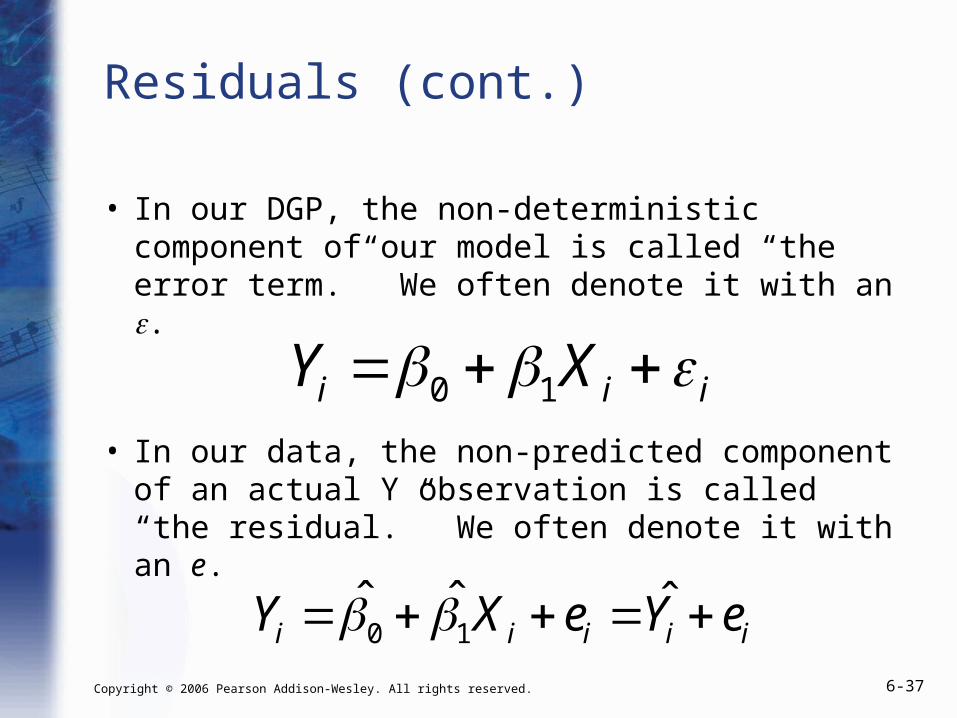
• In our DGP, the non-deterministic component of our model is called “the error term.” We often denote it with an .
• In our data, the non-predicted component of an actual Y observation is called “the residual.” We often denote it with an e.
0 1i i iY X
0 1ˆ ˆ ˆ
i i i i iY X e Y e
Copyright © 2006 Pearson Addison-Wesley. All rights reserved. 6-38
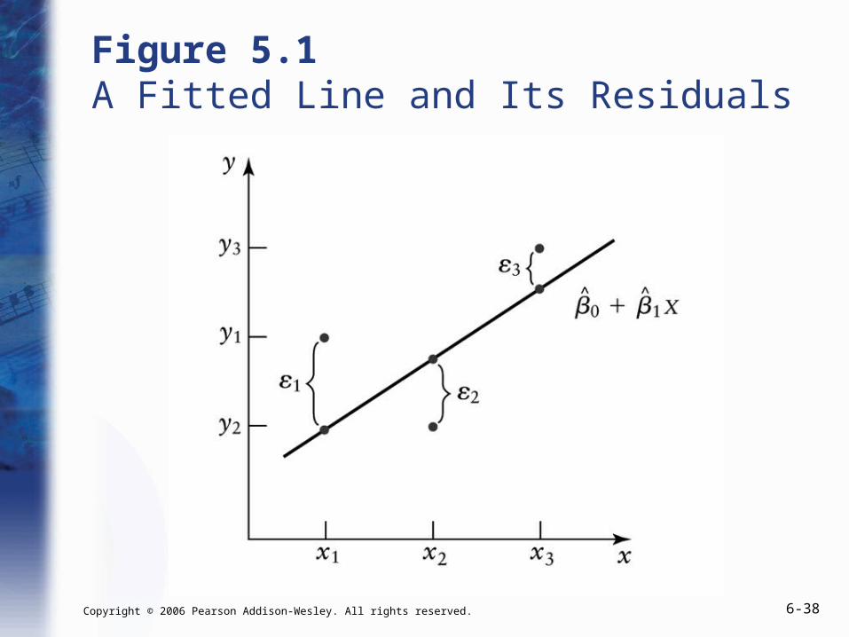
Figure 5.1 A Fitted Line and Its Residuals
Copyright © 2006 Pearson Addison-Wesley. All rights reserved. 6-39
0 1
0 1ˆ ˆ
i i i
i i i
Y X
Y X e
Residuals
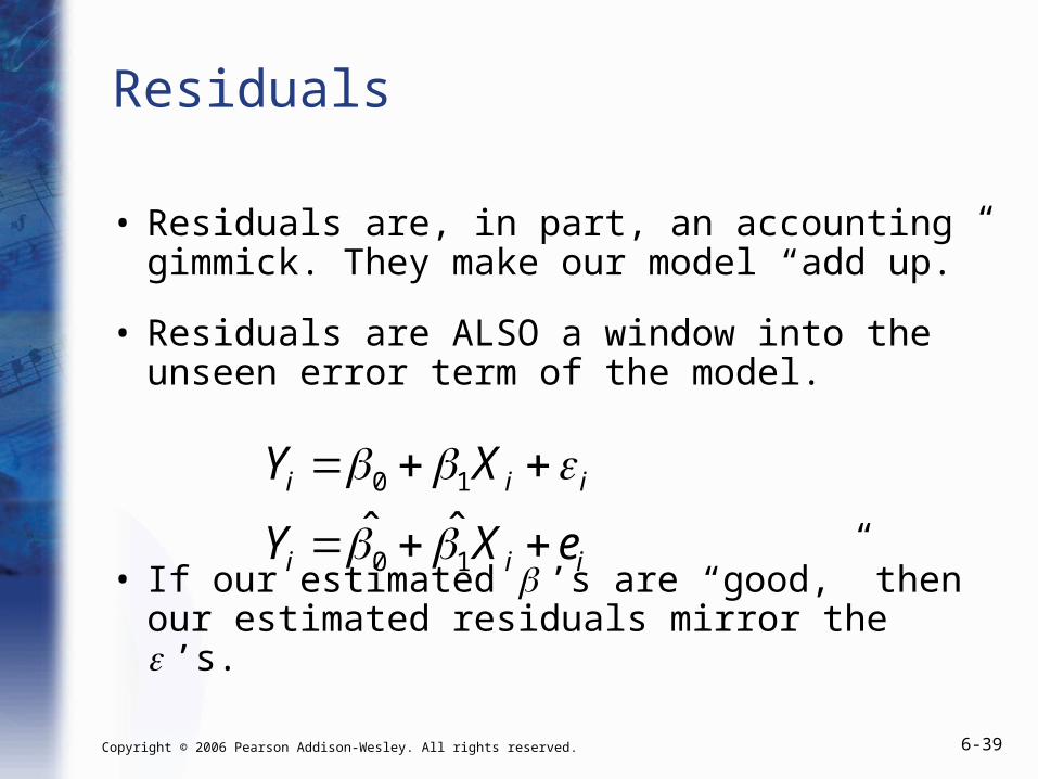
• Residuals are, in part, an accounting gimmick. They make our model “add up.”
• Residuals are ALSO a window into the unseen error term of the model.
• If our estimated ’s are “good,” then our estimated residuals mirror the ’s.

Copyright © 2006 Pearson Addison-Wesley. All rights reserved. 6-40
Residuals (cont.)
• We can use the residuals to tell us something about the error terms.
• So what? The error terms are random and vary from sample to sample. We already KNOW they average to 0.
• What we DON’T know is the VARIANCE of the error terms, 2.
Copyright © 2006 Pearson Addison-Wesley. All rights reserved. 6-41
2
2
1
1( ) ( )
n
i ii
Varn
2 2
1
1( )
n
ii
s e en
Residuals (cont.)
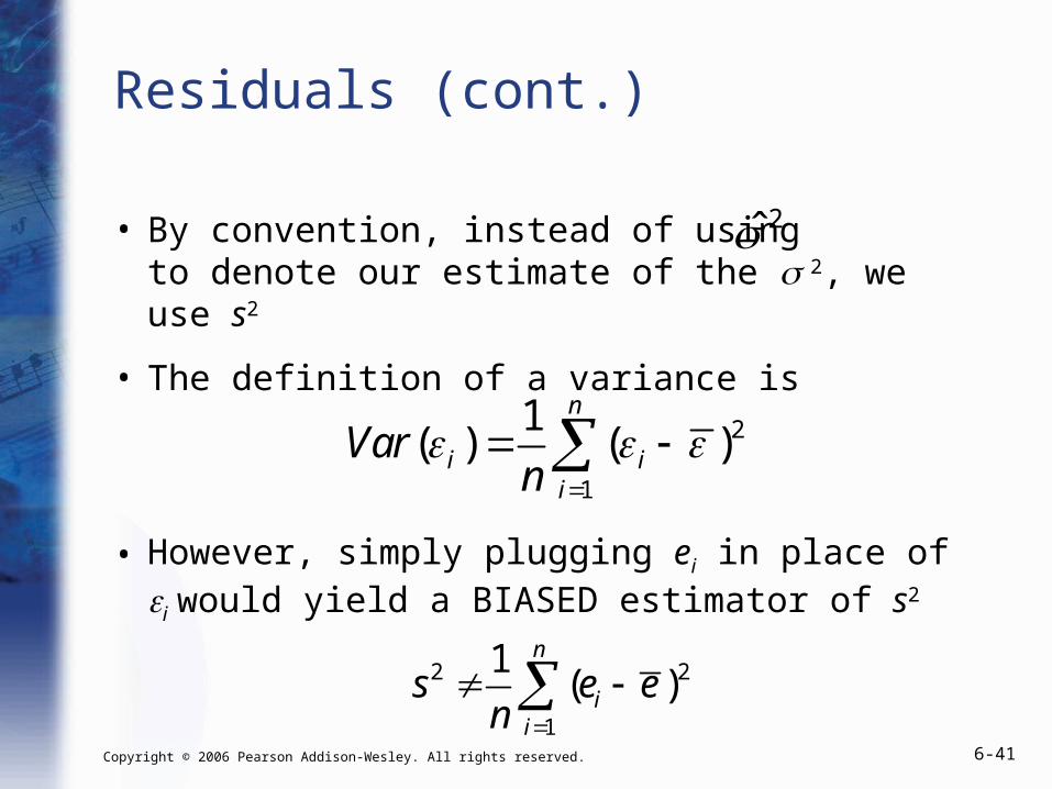
• By convention, instead of using to denote our estimate of the 2, we use s2
• The definition of a variance is
• However, simply plugging ei in place of i would yield a BIASED estimator of s2
Copyright © 2006 Pearson Addison-Wesley. All rights reserved. 6-42
Residuals (cont.)
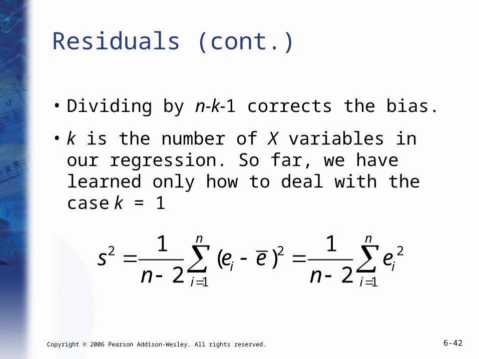
• Dividing by n-k-1 corrects the bias.
• k is the number of X variables in our regression. So far, we have learned only how to deal with the case k = 1
2 2 2
1 1
1 1( )
2 2
n n
i ii i
s e e en n

Copyright © 2006 Pearson Addison-Wesley. All rights reserved. 6-43
Residuals (cont.)
2 2
1
20 1
1
1
2
1 ˆ ˆ( )2
n
ii
n
i ii
s en
Y Xn
Copyright © 2006 Pearson Addison-Wesley. All rights reserved. 6-44
Residuals (cont.)
• Once we have estimated s2, we can use it to estimate the variance of our estimator.
• Then we can use that estimated variance to compute Confidence Intervals, which are a guide to the precision of our estimates.
Copyright © 2006 Pearson Addison-Wesley. All rights reserved. 6-45
Estimating an Estimator’s Variance(Chapter 5.2)
• We chose OLS as our Best Linear Unbiased Estimator because it is unbiased and efficient (for the Gauss–Markov DGP):
– Unbiased: the estimate is “right” in expectation
– Efficient: the estimator has the lowest possible variance
• Our variance is the lowest possible, but what is that variance?
Copyright © 2006 Pearson Addison-Wesley. All rights reserved. 6-46
Estimating an Estimator’s Variance (cont.)
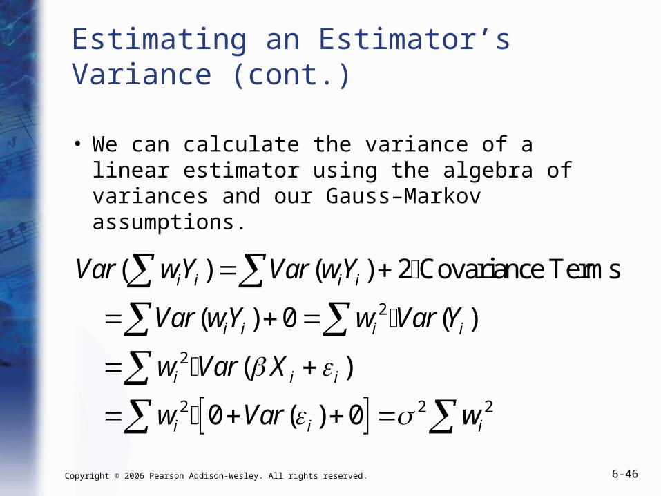
• We can calculate the variance of a linear estimator using the algebra of variances and our Gauss–Markov assumptions.
2
2
2 2 2
( ) ( ) 2 Covariance Terms
( ) 0 ( )
( )
0 ( ) 0
i i i i
i i i i
i i i
i i i
Var wY Var wY
Var wY w Var Y
w Var X
w Var w
Copyright © 2006 Pearson Addison-Wesley. All rights reserved. 6-47
Example: The Phillips Curve
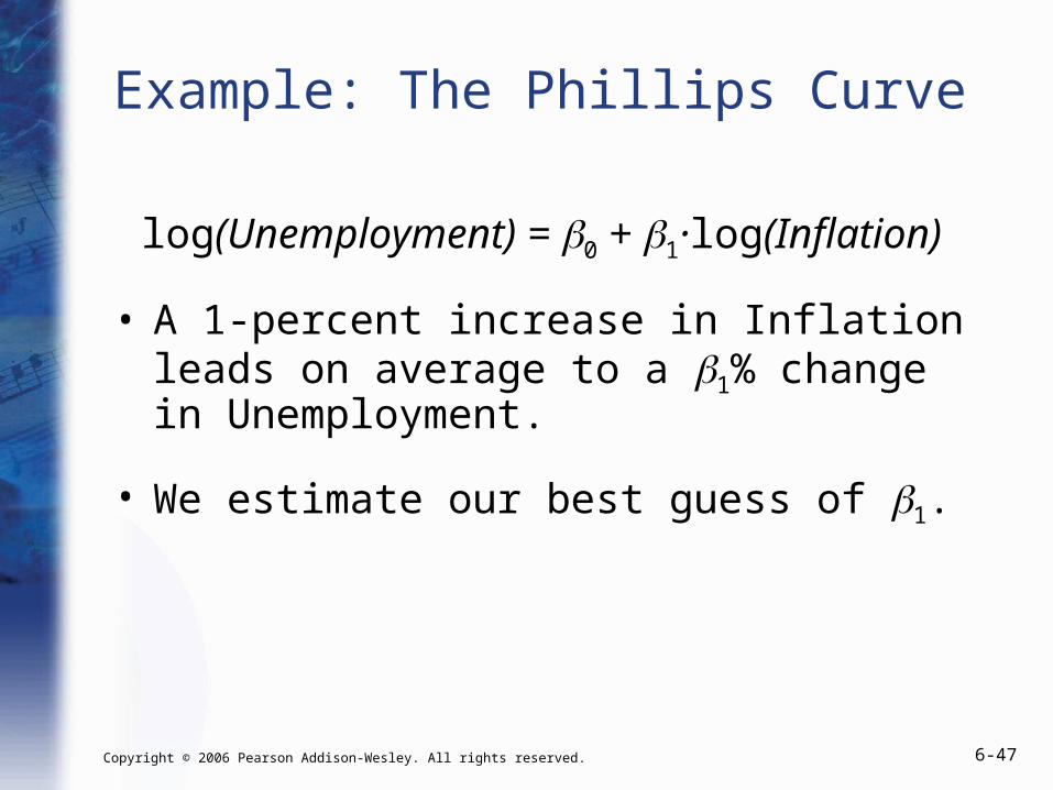
log(Unemployment) = 0 + 1·log(Inflation)
• A 1-percent increase in Inflation leads on average to a 1% change in Unemployment.
• We estimate our best guess of 1.
Copyright © 2006 Pearson Addison-Wesley. All rights reserved. 6-48
TABLE 4.2 A Logarithmic Phillips Curve
Copyright © 2006 Pearson Addison-Wesley. All rights reserved. 6-49
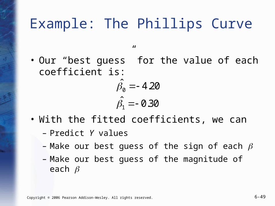
Example: The Phillips Curve
• Our “best guess” for the value of each coefficient is:
• With the fitted coefficients, we can– Predict Y values
– Make our best guess of the sign of each – Make our best guess of the magnitude of each
0
1
ˆ 4.20
ˆ 0.30
Copyright © 2006 Pearson Addison-Wesley. All rights reserved. 6-50
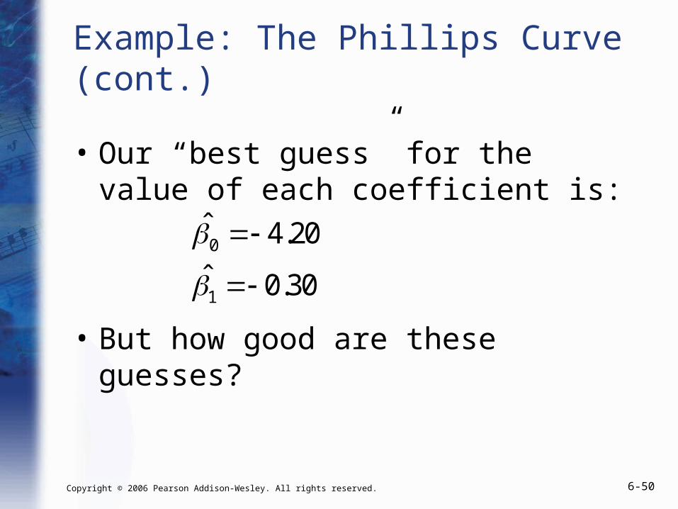
Example: The Phillips Curve (cont.)
• Our “best guess” for the value of each coefficient is:
• But how good are these guesses?
0
1
ˆ 4.20
ˆ 0.30
Copyright © 2006 Pearson Addison-Wesley. All rights reserved. 6-51
Example: The Phillips Curve (cont.)
• We cannot know exactly how good our estimates are, because we do not know the true parameter values (or else we wouldn’t need to estimate them!)
• We know our estimates are right “on average.”
• To gauge how far off our individual estimator could be, we need to estimate the variance of the linear estimator.
Copyright © 2006 Pearson Addison-Wesley. All rights reserved. 6-52
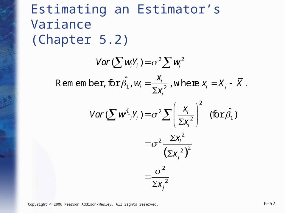
Estimating an Estimator’s Variance(Chapter 5.2)
1
2 2
2
2ˆ 2
2
22
22
2
2
( )
ˆ .
ˆ( ) )
i i i
ii i i
i
ii i
i
i
j
j
Var wY w
xw x X X
x
xVar w Y
x
x
x
x
1
1
Remember, for , , where
(for
Copyright © 2006 Pearson Addison-Wesley. All rights reserved. 6-53
Estimating an Estimator’s Variance (cont.)
• We can calculate xi2 directly.
• The other component of the variance of the estimator is 2, the variance of the error term.
Copyright © 2006 Pearson Addison-Wesley. All rights reserved. 6-54
Estimating an Estimator’s Variance (cont.)
• We do not observe the error terms directly, so we cannot calculate their variance directly
• However, we can proxy for 2 using s2
Copyright © 2006 Pearson Addison-Wesley. All rights reserved. 6-55
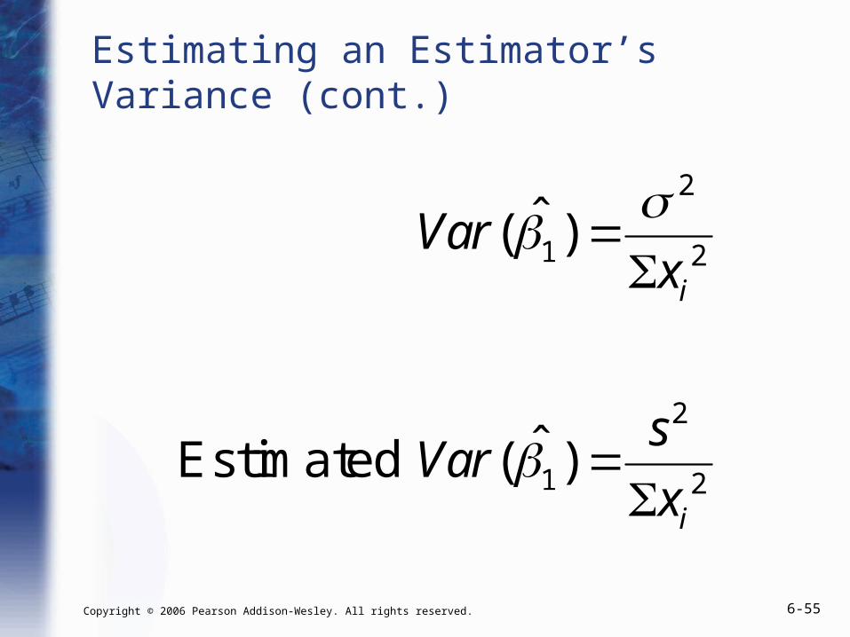
Estimating an Estimator’s Variance (cont.)
2
1 2
2
1 2
ˆ( )
ˆ( )
i
i
Varx
sVar
x
Estimated
Copyright © 2006 Pearson Addison-Wesley. All rights reserved. 6-56
Estimating an Estimator’s Variance (cont.)
• In practice, we typically use not the variance of the estimator, but the standard deviation of the estimator.
• By convention, the standard deviation of an estimator is referred to as the “standard error.”

Copyright © 2006 Pearson Addison-Wesley. All rights reserved. 6-57
Estimating an Estimator’s Variance (cont.)
2
1 2
2
1 2
ˆ. .( )
ˆ. .( )
i
i
s ex
ss e
x
Estimated
Copyright © 2006 Pearson Addison-Wesley. All rights reserved. 6-58
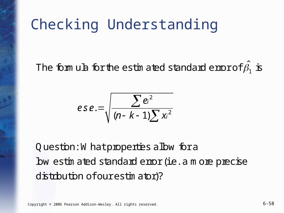
Checking Understanding
2
2
ˆ
. . .( 1)
i
i
ee s e
n k x
1The formula for the estimated standard error of is
Question: What properties allow for a
low estimated standard error (i.e. a more precise
distribution of our estimator)?

Copyright © 2006 Pearson Addison-Wesley. All rights reserved. 6-59
Checking Understanding (cont.)
2
2. . .
( 1)
i
i
ee s e
n k x
1. If the residuals have a lower variance,
e.s.e.’s will be lower. Efficient estimators have the lowest possible ei
2
2. The higher our sample size n, the lower the e.s.e. Bigger samples are better.

Copyright © 2006 Pearson Addison-Wesley. All rights reserved. 6-60
Checking Understanding (cont.)
2
2. . .
( 1)
i
i
ee s e
n k x
3. The fewer parameters we’re estimating,
all else equal, the lower our estimated standard errors.
4. The more broadly our X variable is dispersed, the lower our standard errors. We need variation in X to get a tight estimate of its coefficient.
Copyright © 2006 Pearson Addison-Wesley. All rights reserved. 6-61
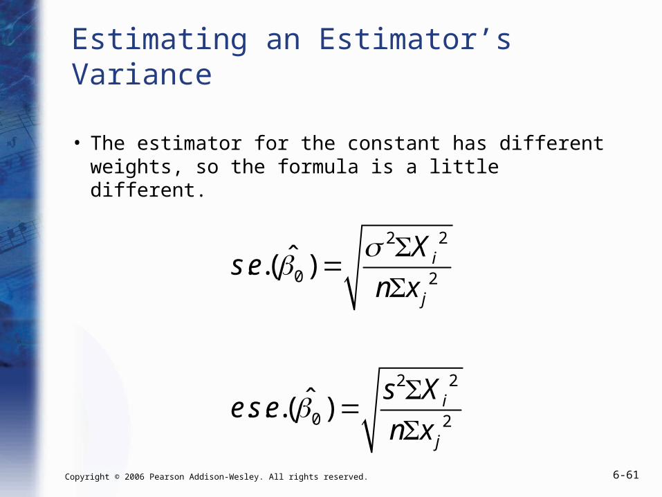
Estimating an Estimator’s Variance
• The estimator for the constant has different weights, so the formula is a little different.
2 2
0 2
2 2
0 2
ˆ. .( )
ˆ. . .( )
i
j
i
j
Xs e
n x
s Xe s e
n x
Copyright © 2006 Pearson Addison-Wesley. All rights reserved. 6-62
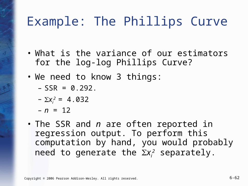
Example: The Phillips Curve
• What is the variance of our estimators for the log-log Phillips Curve?
• We need to know 3 things:– SSR = 0.292.
– xi2 = 4.032
– n = 12
• The SSR and n are often reported in regression output. To perform this computation by hand, you would probably need to generate the xi
2 separately.
Copyright © 2006 Pearson Addison-Wesley. All rights reserved. 6-63
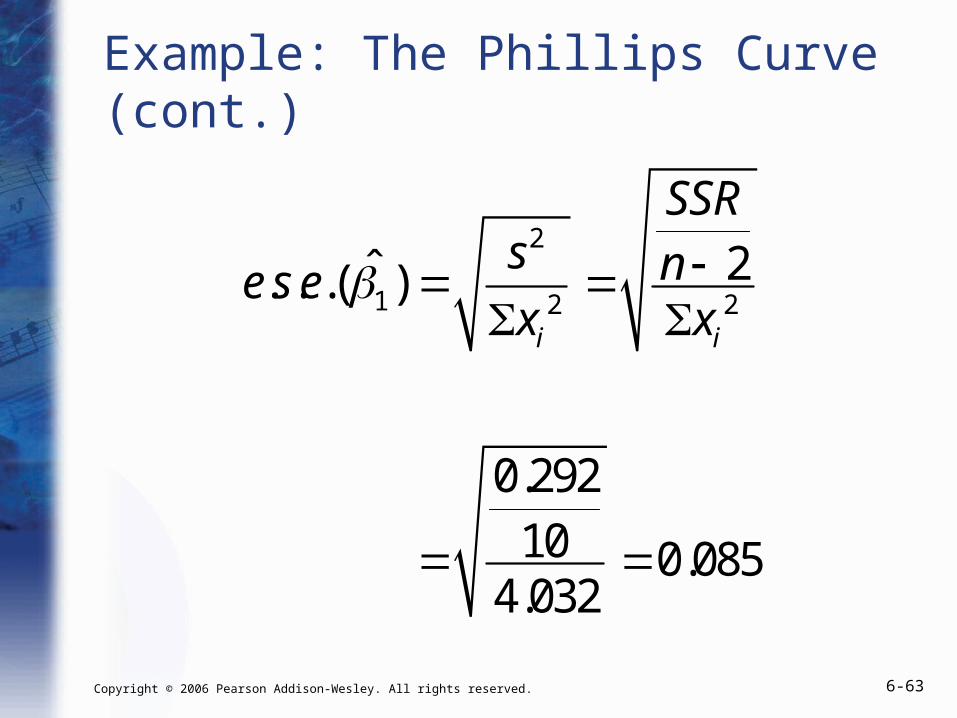
Example: The Phillips Curve (cont.)
2
1 2 22ˆ. . .( )
0.29210 0.085
4.032
i i
SSRs ne s ex x

Copyright © 2006 Pearson Addison-Wesley. All rights reserved. 6-64
TABLE 4.2 A Logarithmic Phillips Curve
Copyright © 2006 Pearson Addison-Wesley. All rights reserved. 6-65
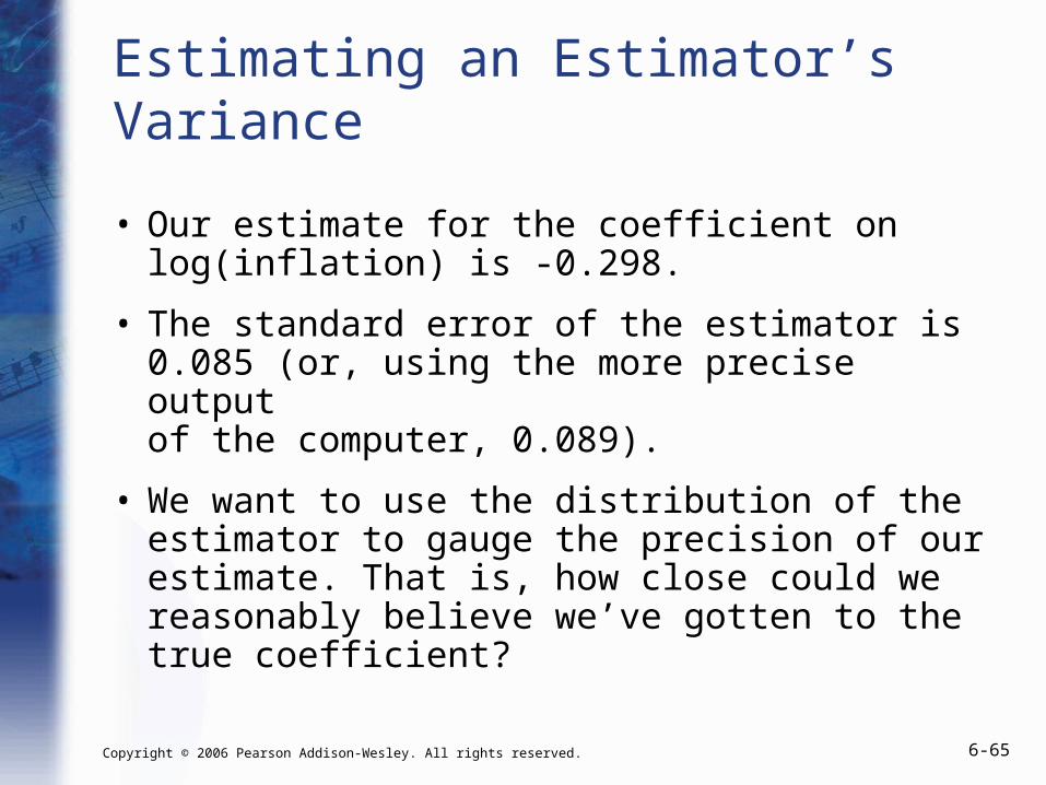
Estimating an Estimator’s Variance
• Our estimate for the coefficient on log(inflation) is -0.298.
• The standard error of the estimator is 0.085 (or, using the more precise output of the computer, 0.089).
• We want to use the distribution of the estimator to gauge the precision of our estimate. That is, how close could we reasonably believe we’ve gotten to the true coefficient?
Copyright © 2006 Pearson Addison-Wesley. All rights reserved. 6-66
Confidence Intervals (Chapter 5.4)
• So far, we have estimated “best guesses.”
• Looking just at “best guesses” though can be a bit misleading. Our “best guess” could be pretty far from the truth.
• We can get a sense of how far off our “best guess” COULD be, by looking at ALL the “good guesses.”
• A “good guess” is a guess with a reasonable chance of being right.
Copyright © 2006 Pearson Addison-Wesley. All rights reserved. 6-67
Confidence Intervals (cont.)
• A “Confidence Interval” is a range of plausible parameter values.
• To interpret Confidence Intervals, we need to think of generating many, many samples from our Data Generating Process.
• For each sample, we observe a C.I.
• Our 95% C.I. will contain the “true” value in 95% of the samples.

Copyright © 2006 Pearson Addison-Wesley. All rights reserved. 6-68
Confidence Intervals (cont.)
• In 95% of samples, our 95% C.I. will contain the “true value.”
• We could also calculate 90% or 99% C.I.’s (or for any other “confidence level”)
• If the C.I. is “wide” (i.e. it contains many values), then it is plausible that our “best guess” estimate is far away from the true value.
Copyright © 2006 Pearson Addison-Wesley. All rights reserved. 6-69
Confidence Intervals (cont.)
• For the Phillips Curve, our “best guess” estimate of the coefficient on log(inflation) is -0.298. A 1% increase in inflation leads to a predicted -0.298% change in unemployment.
• The 95% C.I. is (-0.496, -0.101).
• We could plausibly guess that the effect was -0.496%, -0.101%, or any number in between.
Copyright © 2006 Pearson Addison-Wesley. All rights reserved. 6-70
Confidence Intervals (cont.)
• For the Phillips Curve, our “best guess” estimate of the coefficient on log(inflation) is -0.298. The 95% C.I. is (-0.496, -0.101).
• Was our estimate precise or not? In practice, whether or not we have “good” precision depends on how precise we need to be for our application. If we get the same policy recommendation for all values in our C.I., then we don’t care much which value is “right.”
Copyright © 2006 Pearson Addison-Wesley. All rights reserved. 6-71
Confidence Intervals (cont.)
• In this case, we probably DO care whether the true value is closer to -0.496 or to -0.101. Decreasing unemployment by 0.496% for a 1% increase in inflation may be a very attractive trade-off, but decreasing it by only 0.101% may be much less attractive.
• Policy makers would probably desire a much more precise estimate.
Copyright © 2006 Pearson Addison-Wesley. All rights reserved. 6-72
Confidence Intervals (cont.)
• For the Phillips Curve, our “best guess” estimate of the coefficient on log(inflation) is -0.298. The 95% C.I. is (-0.496, -0.101).
• Our estimate is right in the middle of the C.I.
• We generate the C.I. by starting with our estimate, and adding a (carefully calculated) “fudge factor.”
Copyright © 2006 Pearson Addison-Wesley. All rights reserved. 6-73
Confidence Intervals (cont.)
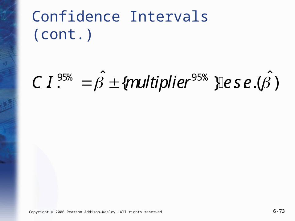
95% ˆ ˆ. . . . .( )C I multiplier e s e 95%{ }

Copyright © 2006 Pearson Addison-Wesley. All rights reserved. 6-74
Confidence Intervals (cont.)
• The starting point for our C.I. is our estimate. Our “best guess” must be a “plausible guess.”
• We then add or subtract a (carefully chosen) multiplier times our estimated standard error.
• The smaller our e.s.e., the tighter our C.I.
• Where does the multiplier come from?
Copyright © 2006 Pearson Addison-Wesley. All rights reserved. 6-75
Confidence Intervals (cont.)
• Our C.I. comes from the distribution of the estimator.
• The estimator follows the “t” distribution. The shape of the t distribution depends on n-k-1. When n-k-1 is very large, the t distribution is approximately the same as the normal distribution.

Copyright © 2006 Pearson Addison-Wesley. All rights reserved. 6-76
Figure SA.11 The Distribution of the t-Statistic Given the Null Hypothesis is True

Copyright © 2006 Pearson Addison-Wesley. All rights reserved. 6-77
Confidence Intervals
% 11
2
ˆ ˆ. . . . .( )n kC I t e s e
Copyright © 2006 Pearson Addison-Wesley. All rights reserved. 6-78
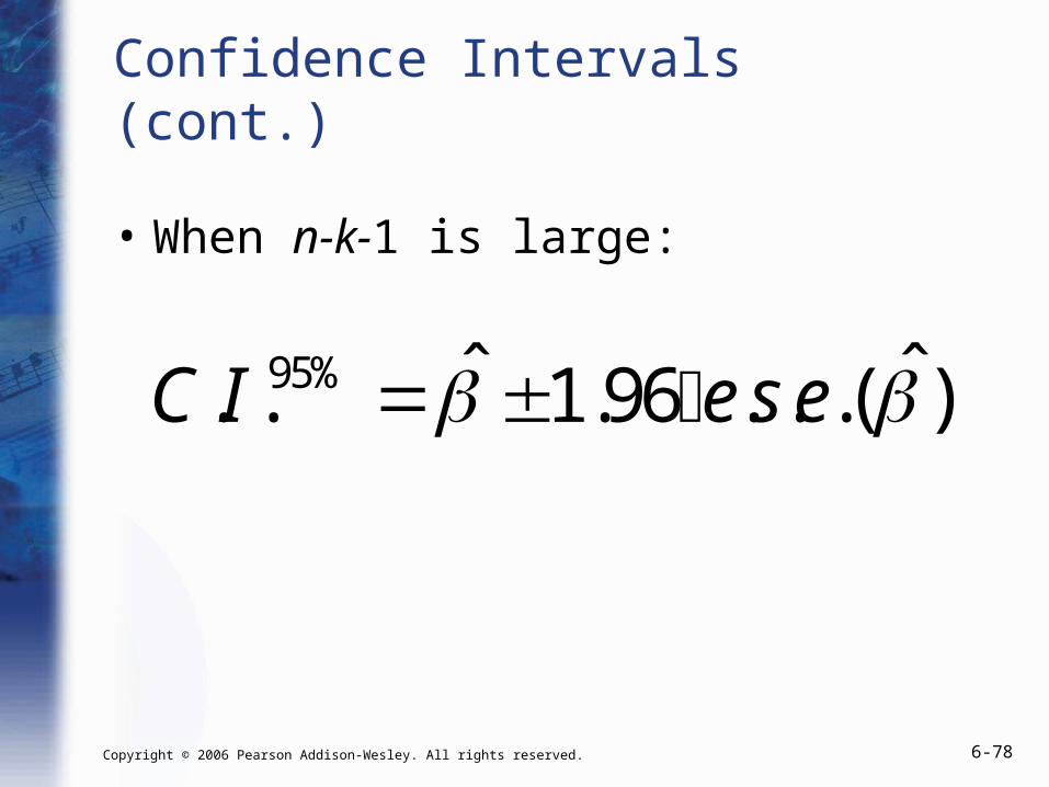
95% ˆ ˆ. . 1.96 . . .( )C I e s e
Confidence Intervals (cont.)
• When n-k-1 is large:
Copyright © 2006 Pearson Addison-Wesley. All rights reserved. 6-79
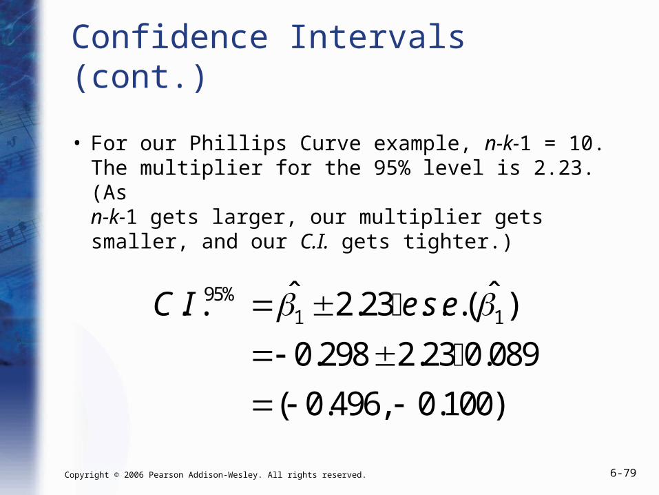
95%1 1
ˆ ˆ. . 2.23 . . .( )
0.298 2.23 0.089
( 0.496, 0.100)
C I e s e
Confidence Intervals (cont.)
• For our Phillips Curve example, n-k-1 = 10. The multiplier for the 95% level is 2.23. (As n-k-1 gets larger, our multiplier gets smaller, and our C.I. gets tighter.)
Copyright © 2006 Pearson Addison-Wesley. All rights reserved. 6-80
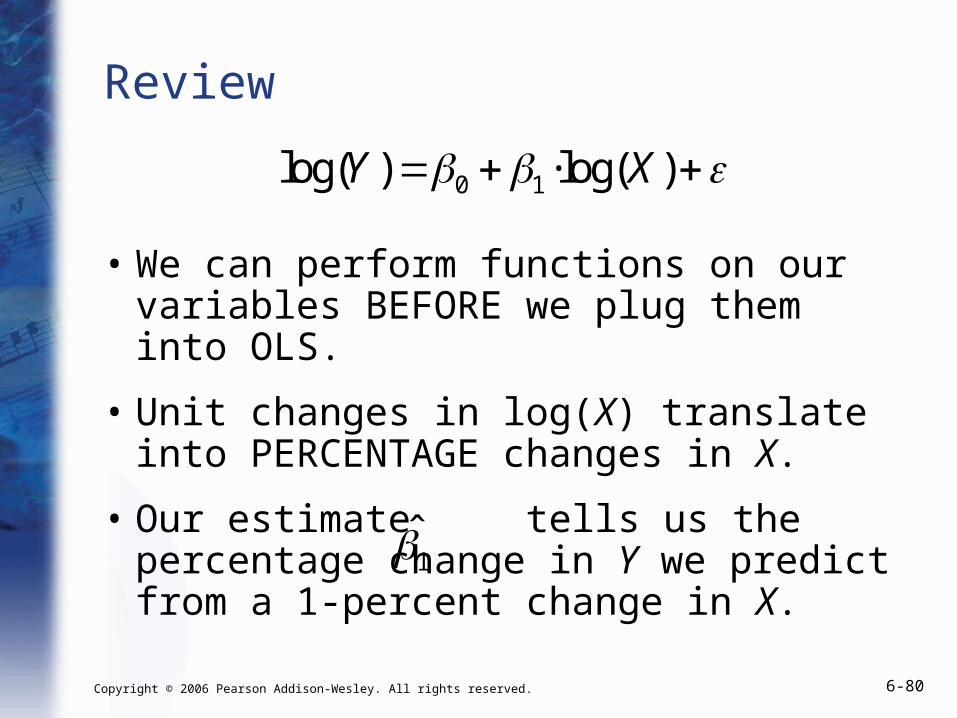
• We can perform functions on our variables BEFORE we plug them into OLS.
• Unit changes in log(X) translate into PERCENTAGE changes in X.
• Our estimate tells us the percentage change in Y we predict from a 1-percent change in X.
1
Review
log(Y ) 0 1·log(X)
Copyright © 2006 Pearson Addison-Wesley. All rights reserved. 6-81
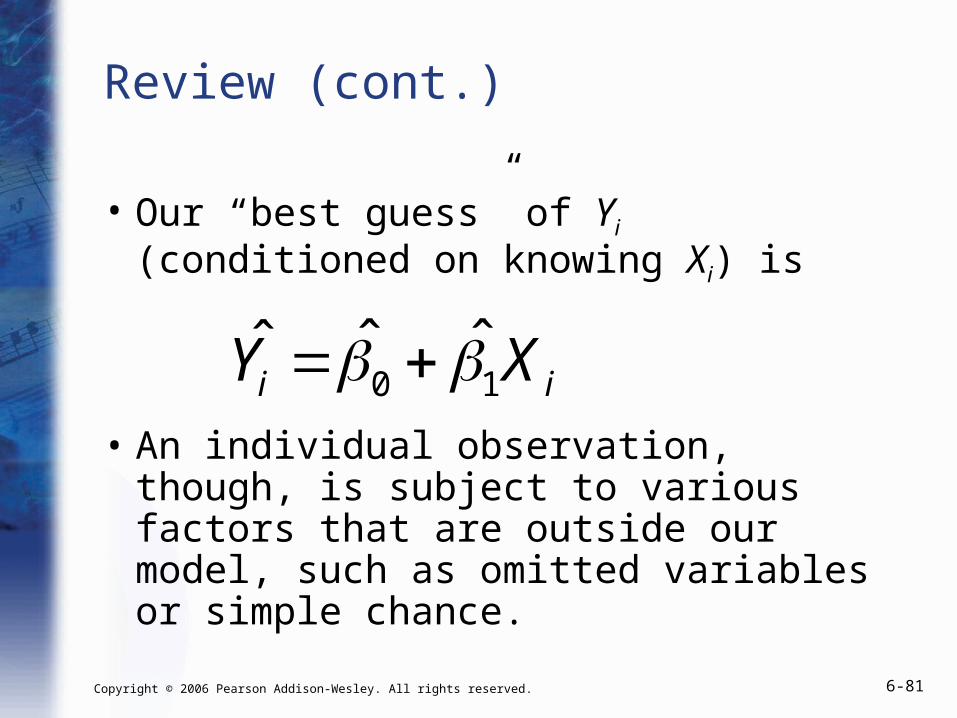
Review (cont.)
• Our “best guess” of Yi (conditioned on knowing Xi) is
• An individual observation, though, is subject to various factors that are outside our model, such as omitted variables or simple chance.
0 1ˆ ˆ
i iY X
Copyright © 2006 Pearson Addison-Wesley. All rights reserved. 6-82
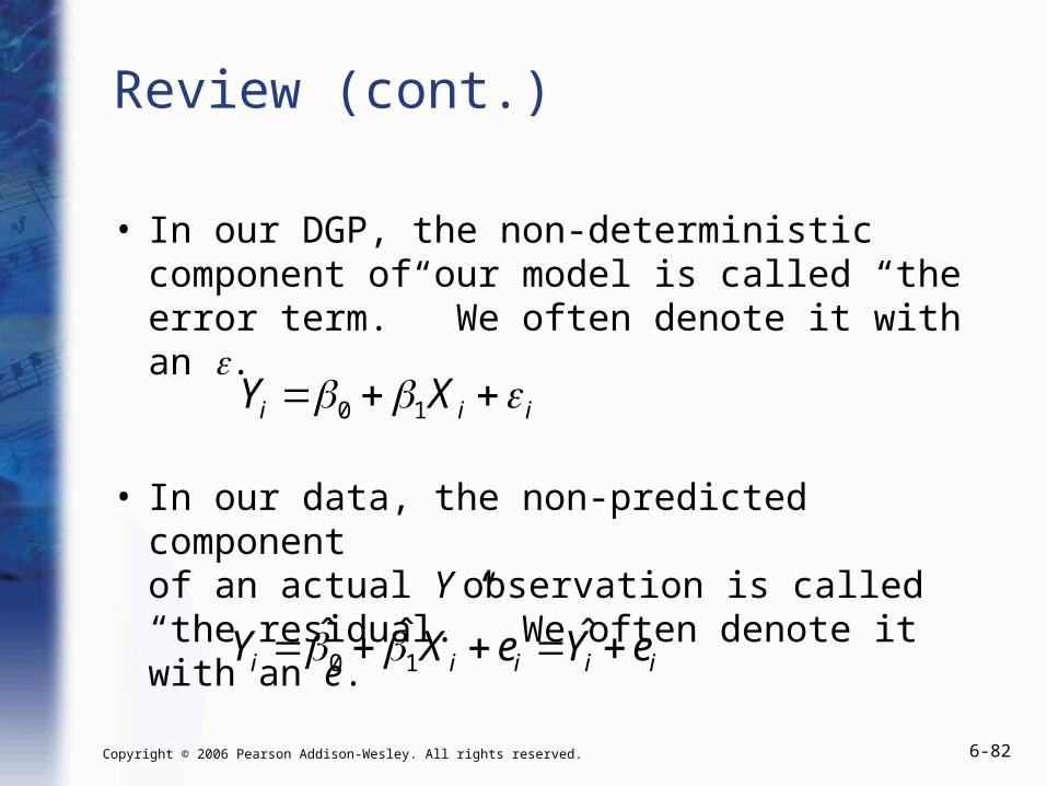
Review (cont.)
• In our DGP, the non-deterministic component of our model is called “the error term.” We often denote it with an .
• In our data, the non-predicted component of an actual Y observation is called “the residual.” We often denote it with an e.
0 1i i iY X
0 1ˆ ˆ ˆ
i i i i iY X e Y e
Copyright © 2006 Pearson Addison-Wesley. All rights reserved. 6-83
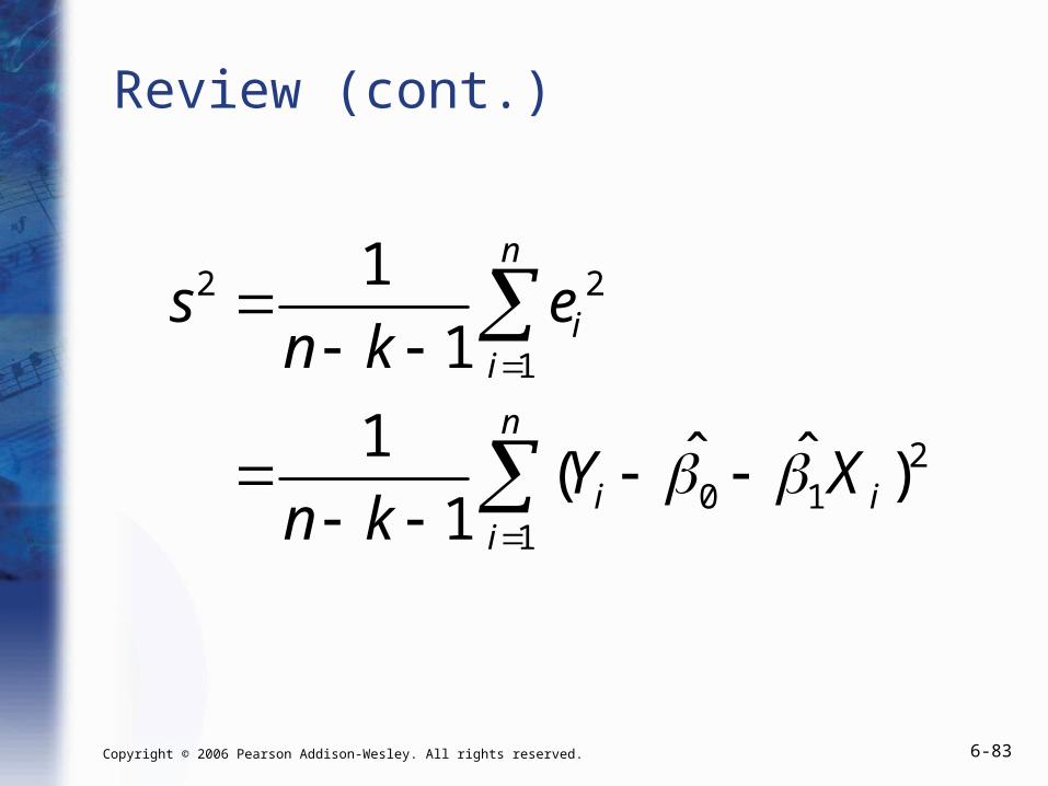
Review (cont.)
2 2
1
20 1
1
1
1
1 ˆ ˆ( )1
n
ii
n
i ii
s en k
Y Xn k
Copyright © 2006 Pearson Addison-Wesley. All rights reserved. 6-84
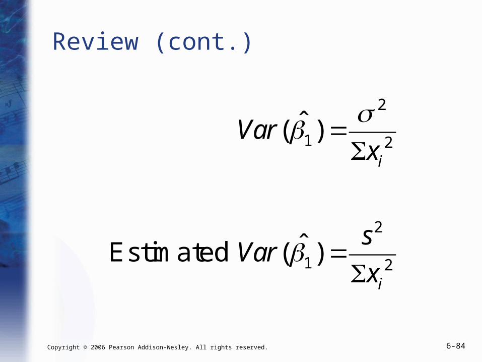
Review (cont.)
2
1 2
2
1 2
ˆ( )
ˆ( )
i
i
Varx
sVar
x
Estimated
Copyright © 2006 Pearson Addison-Wesley. All rights reserved. 6-85
Review (cont.)
• In practice, we typically use not the variance of the estimator, but the standard deviation of the estimator.
• By convention, the standard deviation of an estimator is referred to as the “standard error.”
Copyright © 2006 Pearson Addison-Wesley. All rights reserved. 6-86
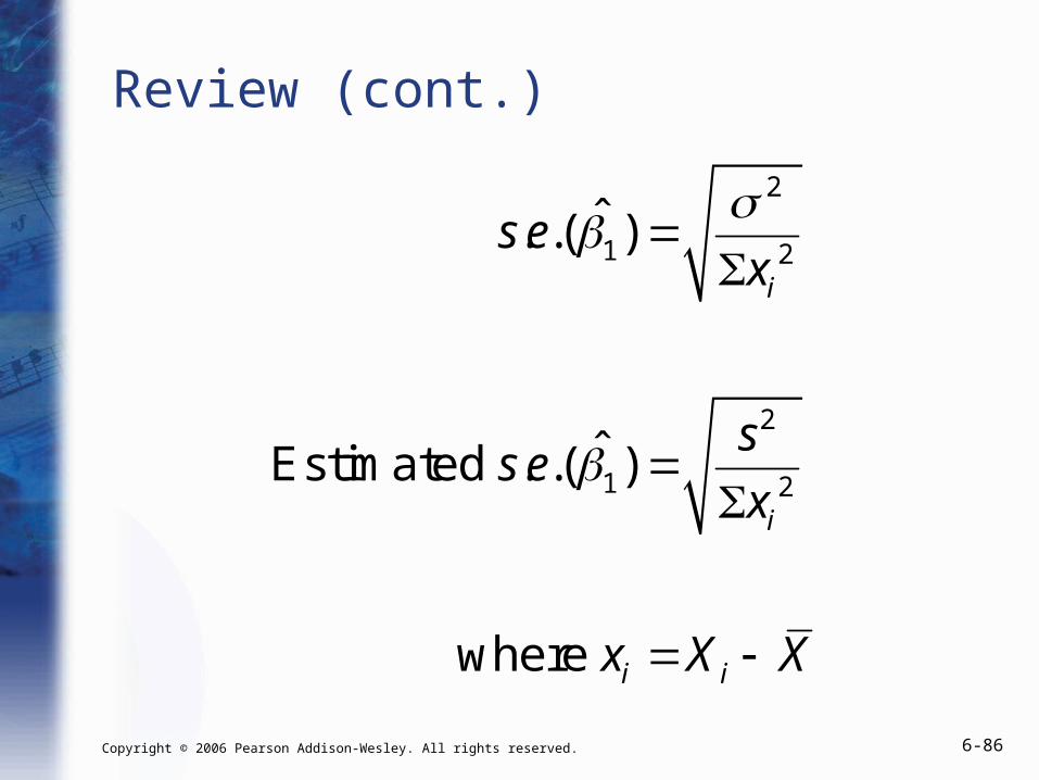
Review (cont.)
2
1 2
2
1 2
ˆ. .( )
ˆ. .( )
i
i
i i
s ex
ss e
x
x X X
Estimated
where
Copyright © 2006 Pearson Addison-Wesley. All rights reserved. 6-87
Review (cont.)
• A “Confidence Interval” is a range of plausible parameter values.
• To interpret Confidence Intervals, we need to think of generating many, many samples from our Data Generating Process.
• For each sample, we observe a C.I.
• Our 95% C.I. will contain the “true” value in 95% of the samples.
Copyright © 2006 Pearson Addison-Wesley. All rights reserved. 6-88
Review (cont.)
• In 95% of samples, our 95% Confidence Interval will contain the “true value.”
• We could also calculate 90% or 99% C.I.’s (or for any other “confidence level”)
• If the C.I. is “wide” (i.e. it contains many values), then it is plausible that our “best guess” estimate is far away from the true value.
Copyright © 2006 Pearson Addison-Wesley. All rights reserved. 6-89
Review (cont.)
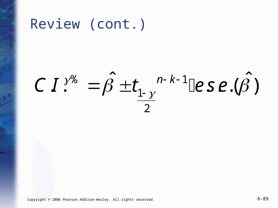
% 11
2
ˆ ˆ. . . . .( )n kC I t e s e