
Cooperative Multi - Robot Explorationmrl.isr.uc.pt/archive/647.pdf · (aap_frontiers) and to...
82
Rui Miguel Pires Carvalho CoopExp Cooperative Multi-Robot Exploration Coimbra 2016
Transcript of Cooperative Multi - Robot Explorationmrl.isr.uc.pt/archive/647.pdf · (aap_frontiers) and to...

Rui Miguel Pires Carvalho
CoopExp Cooperative Multi-Robot Exploration
Coimbra 2016


CoopExpCooperative Multi-Robot Exploration
Rui Miguel Pires Carvalho
Coimbra, September 2016


CoopExpCooperative Multi-Robot Exploration
Supervisor:
Prof. Doutor Rui Paulo Pinto da Rocha
Jury:
Prof. Doutor Rui Pedro Duarte Cortesão
Prof. Doutor Sérgio Paulo Carvalho Monteiro
Prof. Doutor Rui Paulo Pinto da Rocha
Dissertation submitted in partial fulfillment for the degree of Master of Science in
Electrical and Computer Engineering.
Coimbra, September 2016

“The most exciting phrase to hear in science, the one that heralds new
discoveries, is not ’Eureka!’ but ’That’s funny...’"— Isaac Asimov
ii

Acknowledgements
Reflecting back on the journey leading to this dissertation, it is evident that such ac-
complishment is impossible without an often implicit support team. In my case, this team
consists of family members, professional colleagues, academic professors, friends, and lab
mates.
Evidently, this dissertation would not be possible without the supporting of my advisor,
Prof. Doutor Rui Rocha, who I have to thank a lot for his support and indications that kept
me on the right track.
Then I would like to thank all my supportive family. My mom, whose unconditional
support, both moral and financial, has always been a significant source of motivation for all
my endeavors, academic or otherwise. To my uncle Luís Rodrigues for the picture in the
cover.
Perhaps as important as family, friends have also contributed, in some way or another, to
the completion of this dissertation and so I would like to highlight and thank the availability
of all of them.
I’d like to also mention the help of my new friends, lab mates, who have always been
available to help me. A special thank, for all the positive interventions in the development
of my work, to Gonçalo Martins and Paulo Ferreira.
Finally I like to thank my girlfriend, Sofia Sacramento, without her support during this
season and specially in the end, all of this would not be possible to achieve.
iii

iv

Resumo
Ao longo dos anos tornou-se percetível a crescente influência da robótica no domínio
humano, com evidências que vão desde aplicações industriais, espaciais e medicinais, bem
como ferramenta de auxílio em ambientes adversos e em tarefas do quotidiano. Muitas
destas aplicações requerem a utilização de uma equipa de vários robôs móveis cooperantes -
Sistemas Cooperativos Multi-Robô (SCRC) - quer para tornar viável a execução de certas
tarefas, quer para melhorar o desempenho obtido com apenas um robô.
Apesar da capacidade de cooperação ser inata ao Homem, no domínio robótico apresenta
uma série de novos desafios: a comunicação, o sincronismo da informação obtida e a fusão
dessa mesma informação.
Quando a cooperação entre múltiplos robôs é aplicada num contexto de exploração os
desafios são acrescidos. É fundamental ter em consideração os custos e a utilidade dessa
mesma exploração.
Esta dissertação pretende apresentar uma solução à problemática supracitada. Para tal
foi desenvolvido um método capaz de atribuir a diferentes robôs comportamentos cooper-
ativos com a finalidade de explorar um ambiente, seguindo uma filosofia de “dividir para
conquistar”.
O CoopExp, pacote com o algoritmo de exploração, foi desenvolvido segundo uma metodolo-
gia distribuída com o intuito de aumentar a resistência a falhas individuais dos agentes de
exploração. Foi assim criado um método capaz de calcular os custos implicados, de forma
mais rápida e eficiente. Foi ainda estabelecida uma abordagem da utilidade de exploração,
baseada num compêndio de técnicas descritas na literatura.
O desenvolvimento deste tipo de programas era praticamente impossível sem serem re-
alizados testes ao seu funcionamento. Na inexistência de um simulador para este tipo de
operações foi desenvolvido o ARENA (cooperAtive multi Robot frontiEr exploratioN simu-
lAtor). Este é composto por um conjunto de novos pacotes especificamente desenvolvidos
para a identificação de fronteiras (aap_frontiers) e para a otimização da simulação, através
v

de simplificações no processo de obtenção dos mapas (aap_mapping) e posterior combinação
dos mesmos, originando o mapa global (aap_map_merger).
Estas soluções foram validadas através de testes em simulação, recorrendo a unidades
móveis equipadas com um LRF (Laser Range Finder). Testes esses que demonstraram a
diminuição do tempo de exploração quando é aumentado o número de robôs, apresentando
um desempenho adequado tanto em termos de escalabilidade como de eficiência na explo-
ração. Foi ainda realizada, com sucesso, a exploração com uma equipa de robôs reais que
comunicam através de uma rede sem fios, de forma a validar o funcionamento prático deste
projeto.
Palavras-chave: cooperação; equipas de robôs; exploração; simulação; ROS;
mapa de custos
vi

Abstract
Over the years the growing influence of robotics in the human domain has been noticeable
from industrial to space and medical applications as well as a tool in adverse environments
and even in everyday tasks. Many of these applications require the use of a team of sev-
eral cooperating mobile robots - Cooperative Multi-Robot System (CMRS) - to make the
execution of certain tasks possible and to improve the performance achieved by only one
robot.
Although the cooperation capacity is innate to humans, the robotic domain features
a number of new challenges: communication, timing of the information obtained and the
merger of that information.
When cooperation among multiple robots is applied in an exploration context challenges
increase. It is essential to take the costs and utility of that exploration into account.
This dissertation aims to present a solution to the aforementioned problem. Therefore, a
method has been developed, capable of assigning to different robots a cooperative behavior
in order to explore an environment, following a philosophy of "divide and conquer".
The CoopExp, package with the operation algorithm, was developed according to a dis-
tributed approach in order to increase resistance to individual failures of the exploration
agents. Accordingly, a method that is able to calculate the costs involved in a faster and
more efficient way, was created. Furthermore, an approach to exploration utility was also
established, based on a compendium of techniques described in the literature.
The development of such programs would have practically been impossible without per-
forming tests on its functioning. In the absence of a simulator for this type of opera-
tion, the ARENA (cooperAtive multi Robot frontiEr exploratioN simulAtor) was devel-
oped. It consists of a set of new packages specifically designed for frontier identification
(aap_frontiers) and to optimize the simulation, through simplifications in the process of
achieving the maps (aap_mapping) and their subsequent combination, yielding the global
map (aap_map_merger).
vii

Such solutions were validated through simulation tests, using mobile units equipped with
a LRF (Laser Range Finder). These tests showed that exploration time decreases when the
number of robots is increased, presenting a proper performance in terms of scalability and
efficiency in exploration. Last but not least, a exploration with a real team of robots was
successfully carried out that was able to communicate through a wireless network in order
to validate the practical functioning of this project.
Keywords: cooperation; teams of robots; exploration; simulation; ROS; costmap
viii

Contents
Acknowledgements iii
Resumo v
Abstract vii
List of Acronyms xi
List of Algorithms xi
List of Figures xv
List of Tables xvii
1 Introduction 1
1.1 Motivation and Challenges . . . . . . . . . . . . . . . . . . . . . . . . . . . . 2
1.2 Document Overview . . . . . . . . . . . . . . . . . . . . . . . . . . . . . . . 3
2 Exploration with Multi-Robot Systems 5
2.1 The Exploration Strategy . . . . . . . . . . . . . . . . . . . . . . . . . . . . 5
2.1.1 Cooperation Strategies . . . . . . . . . . . . . . . . . . . . . . . . . . 6
2.2 Related Work . . . . . . . . . . . . . . . . . . . . . . . . . . . . . . . . . . . 7
2.2.1 Comparison of Approaches . . . . . . . . . . . . . . . . . . . . . . . . 10
2.3 Robot Operating System . . . . . . . . . . . . . . . . . . . . . . . . . . . . . 11
2.3.1 Useful ROS Packages for Multi-Robot Explorations . . . . . . . . . . 12
2.4 Pioneer 3-DX Robot . . . . . . . . . . . . . . . . . . . . . . . . . . . . . . . 15
2.5 Summary . . . . . . . . . . . . . . . . . . . . . . . . . . . . . . . . . . . . . 16
3 ARENA - The Simulator 17
3.1 The Need for a Simulator . . . . . . . . . . . . . . . . . . . . . . . . . . . . 17
ix

3.2 An Overview of ARENA . . . . . . . . . . . . . . . . . . . . . . . . . . . . . 17
3.3 Stage, RViz and Move_Base Configurations . . . . . . . . . . . . . . . . . . 18
3.4 Map Merging with Matching Maps . . . . . . . . . . . . . . . . . . . . . . . 19
3.5 Localization . . . . . . . . . . . . . . . . . . . . . . . . . . . . . . . . . . . . 22
3.6 Frontier Generation Node . . . . . . . . . . . . . . . . . . . . . . . . . . . . 24
3.7 Summary . . . . . . . . . . . . . . . . . . . . . . . . . . . . . . . . . . . . . 27
4 CoopExp - Exploration Algorithm 29
4.1 The Costmap Generation . . . . . . . . . . . . . . . . . . . . . . . . . . . . . 30
4.1.1 Classification of Costmap Algorithms . . . . . . . . . . . . . . . . . . 35
4.2 The Utility of a Frontier Cell . . . . . . . . . . . . . . . . . . . . . . . . . . 37
4.2.1 Proximity of Frontier cells . . . . . . . . . . . . . . . . . . . . . . . . 37
4.2.2 Minimum Distance to Other Robots . . . . . . . . . . . . . . . . . . 39
4.3 Goal Generation . . . . . . . . . . . . . . . . . . . . . . . . . . . . . . . . . . 41
4.4 Summary . . . . . . . . . . . . . . . . . . . . . . . . . . . . . . . . . . . . . 42
5 Validation and Results 43
5.1 ARENA Performance . . . . . . . . . . . . . . . . . . . . . . . . . . . . . . . 43
5.2 CoopExp Experimentation . . . . . . . . . . . . . . . . . . . . . . . . . . . . 45
5.2.1 Gains Calibration . . . . . . . . . . . . . . . . . . . . . . . . . . . . . 45
5.2.2 Efficiency in Simulated Environments . . . . . . . . . . . . . . . . . . 47
5.2.3 Real-World Validation . . . . . . . . . . . . . . . . . . . . . . . . . . 51
5.3 Summary . . . . . . . . . . . . . . . . . . . . . . . . . . . . . . . . . . . . . 52
6 Conclusion 53
6.1 Future Work . . . . . . . . . . . . . . . . . . . . . . . . . . . . . . . . . . . . 54
7 Bibliography 57
x

List of Acronyms
ARENA cooperAtive multi Robot frontiEr exploratioN simulAtor
CMRS Cooperative Multi-Robot System
CPU Central Processing Unit
ISR Institute of Systems and Robotics
GUI Graphical User Interface
LRF Laser Range Finder
LTS Long Term Support
MAS Multi-Agent System
MRS Multi-Robot System
NFE Near Frontier Exploration
SLAM Simultaneous Localization and Mapping
ROS Robot Operating System
2D Two-Dimensional
xi

xii

List of Algorithms
3.1 Update function of Global Map . . . . . . . . . . . . . . . . . . . . . . . . . . 21
3.2 Update Frontiers Map . . . . . . . . . . . . . . . . . . . . . . . . . . . . . . . 25
3.3 Frontier identification algorithm . . . . . . . . . . . . . . . . . . . . . . . . . 26
3.4 Inflame Obstacles . . . . . . . . . . . . . . . . . . . . . . . . . . . . . . . . . 26
4.1 Costmap Initialization Function. . . . . . . . . . . . . . . . . . . . . . . . . . 31
4.2 Costmap Update Function. . . . . . . . . . . . . . . . . . . . . . . . . . . . . 32
4.3 Find Next Starting Point. . . . . . . . . . . . . . . . . . . . . . . . . . . . . . 33
4.4 Minimum Cost Function. . . . . . . . . . . . . . . . . . . . . . . . . . . . . . 34
4.5 Number of nearby frontiers. . . . . . . . . . . . . . . . . . . . . . . . . . . . . 40
4.6 Minimum distance to other robots. . . . . . . . . . . . . . . . . . . . . . . . . 40
xiii

xiv

List of Figures
2.1 Detection of frontier cells and regions [39]. . . . . . . . . . . . . . . . . . . . 7
2.2 Typical costmaps obtained for two different robot positions [5]. . . . . . . . . 8
2.3 Hill climbing exploration of a typical office environment by a single mobile
robot equipped with a ring of 16 sonars [31]. . . . . . . . . . . . . . . . . . . 9
2.4 Example of a ROS rqt-graph. . . . . . . . . . . . . . . . . . . . . . . . . . . . 12
2.5 An example of a multi-robot simulation using the package RViz as a GUI. . 12
2.6 Stage GUI of a two robots simulation. . . . . . . . . . . . . . . . . . . . . . 13
2.7 Example of a map generated with gmapping. . . . . . . . . . . . . . . . . . . 14
2.8 A high-level view of the move_base node [10]. . . . . . . . . . . . . . . . . . 14
2.9 Example of a Pioneer 3-DX. . . . . . . . . . . . . . . . . . . . . . . . . . . . 15
3.1 Modes of operation present in mrgs_slam [23]. . . . . . . . . . . . . . . . . . 19
3.2 Map merging scenario in the beginning of a multi-robot map operation. . . . 22
3.3 Progressive growth of a map using the aap_mapping package. . . . . . . . . 23
3.4 An example of a frontier map generated from a local map of a robot. . . . . 25
4.1 An example of a costmap generated with the spiral sweeping algorithm. . . . 35
4.2 An illustration of a map with 8 u-turns (forced reversal). . . . . . . . . . . . 35
4.3 A graphical comparison between the two Big O classifications, O(cn1.5) and
O(2cn). . . . . . . . . . . . . . . . . . . . . . . . . . . . . . . . . . . . . . . 36
4.4 Frontier cells line in a wide area. . . . . . . . . . . . . . . . . . . . . . . . . . 38
4.5 Frontier cells line in a hall. . . . . . . . . . . . . . . . . . . . . . . . . . . . . 39
4.6 An example of a proximity case between two robots. . . . . . . . . . . . . . . 41
5.1 An example of a simulation with 16 robots using ARENA . . . . . . . . . . . 44
5.2 A graphical illustration of a CPU load in function of the number of robots in
a Quad-Core computer. . . . . . . . . . . . . . . . . . . . . . . . . . . . . . . 44
xv

5.3 A graphical illustration of a CPU load in function of the number of robots in
a Dual-Core computer. . . . . . . . . . . . . . . . . . . . . . . . . . . . . . . 45
5.4 Grid map for gains calibration. . . . . . . . . . . . . . . . . . . . . . . . . . 46
5.5 A graphical illustration of the results obtained in each set of the alpha cali-
bration. . . . . . . . . . . . . . . . . . . . . . . . . . . . . . . . . . . . . . . 47
5.6 A graphical illustration of the results obtained in each set of the beta calibration. 47
5.7 Different environments for simulation with multiple robots. . . . . . . . . . . 48
5.8 A graphical illustration of multiple experiences performed in four different
simulated environments using ARENA . . . . . . . . . . . . . . . . . . . . . 48
5.9 A graphical illustration of the experience performed in the Grid environment. 49
5.10 A graphical illustration of the experience performed in the Big room environ-
ment. . . . . . . . . . . . . . . . . . . . . . . . . . . . . . . . . . . . . . . . . 49
5.11 A graphical illustration of the experience performed in the Triple u-turn en-
vironment. . . . . . . . . . . . . . . . . . . . . . . . . . . . . . . . . . . . . . 50
5.12 A graphical illustration of the experience performed in the Office floor envi-
ronment. . . . . . . . . . . . . . . . . . . . . . . . . . . . . . . . . . . . . . . 50
5.13 A small experience set up for real world validation in ISR. . . . . . . . . . . 51
5.14 An illustration of the frontiers map resulting of both the real and simulated
explorations. . . . . . . . . . . . . . . . . . . . . . . . . . . . . . . . . . . . . 52
xvi

List of Tables
2.1 Comparative table of the differences between the methods of Yamauchi, Bur-
gard, Rocha, André and Colares. . . . . . . . . . . . . . . . . . . . . . . . . 10
3.1 Maps notations. . . . . . . . . . . . . . . . . . . . . . . . . . . . . . . . . . . 20
4.1 Cell values notation for the costmap value c, utility value u and final explo-
ration value v. . . . . . . . . . . . . . . . . . . . . . . . . . . . . . . . . . . . 29
xvii

xviii

1 Introduction
The exploration of unknown environments with robots is a fundamental problem in mobile
robotics. There are several applications in different areas, such as planetary exploration [25]
[14], demining [4] [11], reconnaissance [26], cleaning [18], search and rescue [22], etc.
This dissertation aims to explore the potentialities of a Multi-Robot System (MRS) [1].
These are a subclass of a Multi-Agent System (MAS), which are distinguished in terms of
efficiency and robustness when applied in overly complex tasks for a single mobile robot.
These capabilities require a high degree of coordination and cooperation between all units
of a MRS and also an efficient communication method [24].
The capabilities cited above, are extremely important in exploration tasks, hence the
adoption of MRS to perform them. For example, a search and rescue operation [32] can
apply the inherent potentialities of robotics with a MRS. Assuming a fire scenario in a
shopping center with several exits, rooms, halls, etc, a team of robots (search team) would
be able to explore the site more quickly and efficiently, obtaining at the same time information
about risk areas and localization of victims. With this data the rescue team (police officers,
firefighters and paramedics) could also be equipped with the necessary information to rescue
victims through the safest route, avoiding the most critical areas of the fire. Thus allowing
the creation of a more effective plan to extinguish the fire and reducing the total damage.
The use of multiple robots significantly reduces the time required to explore the envi-
ronment and this reduction is proportional to the number of robots used [5]. To explore
an environment different methods can be used such as the Voronoi diagrams [38], Potential
information fields [35], Harmonic functions [9], the Frontiers based exploration method [39]
which is the one used in this dissertation, among others [3] [6] .
An exploration requires that the robots are provided with a method for Simultaneous
Localization and Mapping (SLAM) [21] allowing the construction of a map of the unknown
environment and its location in relation to that map. To build a map, the environment is
divided into cells and each cell represents an area of that environment. Therefore, through-
1

out the exploration new areas are discovered and the map is filled. From this point onwards
the necessary information is gathered for the frontier identification. A frontier represents
the boundary between known and unknown areas, and it is necessary to select and allocate
different frontiers to the available robots. Allocating tasks to available resources is an op-
timization problem, which is similar to what happens when assigning frontiers to robots,
making the exploration algorithm a solution for this optimization problem.
1.1 Motivation and Challenges
The purpose of this dissertation is to study multi-robot exploration techniques and to
implement a solution for the existing mobile robot fleet in the Institute of Systems and
Robotics (ISR) - University of Coimbra.
Building a metric map of the environment is both an objective and a challenge for this
work. It is motivating to know that it will be easy to add more sensors to the robots and
record more information throughout the exploration. For example, in search and rescue
operations, the robot could map different variables such as temperature, smoke density or
concentration of explosive and/or toxic substances, and detect the focus of the fire and the
presence of victims.
To ensure scalability and resilience of the robotic system in relation to individual faults or
limitations in wireless communication, there should be favored solutions based on distributed
decisions.
On the other hand, assigning the ability to cooperate to a group of robots is both a
challenge and a motivation. There can be many rules in an exploration to steer the robots.
One rule can have a negative influence on another, so it is necessary to weigh out the
influence of each in order to always get the best possible goal. This represents a challenge
since it is impossible to set a rule for every scenario. To work around this problem various
combinations of rules with different influences in multiple scenarios were tested. Due to the
high number of tests required for optimization of rules and influences, the use of a simulator
becomes indispensable.
The lack of a specific simulator for the operation was evident from the beginning and be-
came a new objective during the development of the exploration algorithm, thus a motivation
for to making it available online as open-source.
2

1.2 Document Overview
This dissertation is divided into six chapters, each referring to a different stage of this
work. Chapter 1 is an introduction and contextualization to the problem and an outline
of both motivations and challenges. Chapter 2 is a compendium of the state of the art of
exploration with a MRS in general and a more specific research in frontier-based exploration.
Also, an overview of Robot Operating System (ROS) was done.
The package of the exploration simulator in ROS with all its auxiliary packages is pre-
sented in chapter 3. Chapter 4 has all the information about the exploration algorithm.
Experimentation and validation of the multi-robot exploration algorithm is presented in
chapter 5.
All findings are finally presented in the last chapter, chapter 6, as well as the prospects
for a future work.
3

4

2 Exploration with Multi-Robot Systems
This chapter presents some of the exploration methods used in robotics, with a deeper
focus on analysis in frontier-based exploration. An overview, of the most important concepts
of ROS related to this project was done.
2.1 The Exploration Strategy
As indicated in chapter 1, there are different methods to guide an exploration with
robots such as Voronoi diagrams, Potential information fields [35], Harmonic functions [9]
or Frontier-based exploration. Within the range of the analyzed methods, Frontier-based
exploration and Voronoi diagrams were the most relevant for this project.
Regarding exploration using the mobile robots, frontiers are inevitably mentioned [19].
The frontier is the boundary of the knowledge of the environment, and so a goal in any
exploration. More specifically, when a map (occupancy grid) is used as the basic space
representation model of the environment, a frontier cell is defined by Yamauchi et al. [39]
as is in definition 2.1.
Definition 2.1. Frontier Cell: Assuming the existence of a map, frontiers cells are the
unknown cells, bordering contiguous to one or more free explored cells [39].
After the identification of all frontier cells, costs and utilities for each cell border are
equated. Then each robot choses its goal taking into account these costs and utilities. The
exploration proceeds while at least one frontier cell exists. This strategy is called frontier-
based exploration.
A Voronoi diagram can also be applied to a robotic exploration [38] since it is a tool
to divide an environment into regions, based on the position of each of the robots that are
exploring (definition 2.2). It is guaranteed that each point contained in these regions is closer
to the robot that originated the region than to any other.
5

Definition 2.2. Voronoi diagram: The partitioning of a plane with n points into convex
polygons such that each polygon contains exactly one generating point and every point in a
given polygon is closer to its generating point than to any other [37].
After the regions are determined a frontier cell is assigned to each robot, but in this case
instead of analyzing the entire map to calculate costs and utilities, it analyzes only the region
of the map assigned to this robot. This method is more efficient for larger maps, however
the selected goal is not always the most suitable, since the complete map is not considered.
This was the reason for the choice of a Frontier-based exploration with a global approach.
2.1.1 Cooperation Strategies
Another issue raised with regarding to explorations with a MRS is the cooperation be-
tween robots [33]. This cooperation can be implemented in many different ways and has
been the topic of much interest (e.g. [13], [12] and [27]). Cooperation is known for increas-
ing efficiency of the exploration, to coordinate, avoid conflicts and redundancies.
To begin, a key aspect of cooperation is the exchange of map information between robots
[20]. This technique enables teams of robots to efficiently explore environments from different
unknown locations, since it allows robots to have an overall knowledge of the environment
[34].
In a decentralized approach, by being able to see each other [30] or by sharing their
position robots, are able to determine the usefulness of exploring the remaining parts of the
environment. Thus allowing for a more intelligent decision when in the position of choosing
a new direction of exploration.
Other approaches take into account the possibilities of a robot collaboration where robots
work together in order to clear blocked paths or any other task, therefore raising the question
of when and with whom to collaborate [2]. Team of robots may have to permanently maintain
an ad-hoc network structure with each other in order to communicate due to constrains
imposed by wireless networking, vital in any cooperative exploration [1]. These restrictions
will limit the movement possibilities of robots and may imply that some robots keep their
position stationary, without making any direct contribution to the exploration.
6

2.2 Related Work
In 1998 Yamauchi et al. [39] developed a technique to coordinate a team of robots with
the aim of building a map through frontier analysis. A frontier cell was not sufficient to
generate a target, which led to the need for a region of frontiers cells, forming a sufficiently
wide area allowing the safe passage of the robot. Only the cells belonging to a region of
frontiers cells were considered as possible targets. The frontier cell belonging to a region of
frontier cells that is closest to the robot is defined as the next target to explore. This method
is known as Near Frontier Exploration (NFE).
(a) evidence grid. (b) frontier segments. (c) frontier regions.
Figure 2.1: Detection of frontier cells and regions [39].
In figure 2.1a there is a graphical representation of the exploration map, where the
thin gray dots represent unknown cells, the thick black dots the obstacles and the white
cells represent free cells. After analyzing this map, the algorithm generates a grid with
the frontier cells (Figure 2.1b) which subsequently form frontier regions and its respective
centroid (Figure 2.1c). This is a cooperative and decentralized approach that assumes the
existence of a line of communication that allows for the robots to share the created maps
among themselves. All robots work desynchronized making the system robust to individual
failures. However, this method turns out to generate redundancies since the same area was
repeatedly assigned to two different robots, which makes it less efficient.
7

Later in 2005, Burgard et al. [5] developed a technique which used the balance between
the cost of achieving a frontier cell and its utility of exploration. The cost of achieving a cell
is calculated using a path planning algorithm, taking known obstacles into consideration.
However, if there are obstacles between robots this can be associated with a very high cost in
spite of the target cell being near the robot. The utility of exploring a frontier cell increases
with the number of nearby frontier cells and decreases with the proximity of other robots.
This last factor introduces a repulsive behavior on robots. Thus, in each iteration, the cost
of getting to a frontier cell and its utility are values calculated in order to predict the optimal
exploration goal, which allows to minimize exploration time.
(a) (b)
Figure 2.2: Typical costmaps obtained for two different robot positions [5]. The blackrectangle indicates the target points in the unknown area with minimum cost.
Through the analysis of figure 2.2 it is possible to observe the exploration goal (black
rectangle), which is entirely generated based on the cost of reaching that goal. This often
results in two robots scaled to the same point. When considering the utility of a frontier
cell, each robot tends to have a different goal, since the utility of a frontier cell decreases
with the proximity of other robots. Despite the clear improvement in the effectiveness of the
exploration, this method is computationally prohibitive when applied in larger environments.
In 2008, Rocha et al. [31] resorted to a local approach rather than the global approach
of Burgard et al. This method is computationally less demanding, which facilitates the
application to mobile robots with lower processing capabilities. However, this approach will
generate local minima problems since it only analyzes an area near the robot. The robot
can reach a position where, in its neighborhood, all cells are explored or inaccessible without
having fully explored the whole environment. To solve this problem the algorithm keeps a
register of previously explored points. In the absence of frontiers in the neighborhood, the
algorithm will analyze previously explored points, starting with the closest (shortest path
algorithm), in order to find the remaining frontiers in the map. Finally, the exploration
8

is assumed to be completed when a frontier is not found, after analyzing all points in its
register.
Figure 2.3: Hill climbing exploration of a typical office environment by a single mobile robotequipped with a ring of 16 sonars [31]. On the left, it is shown the topological map (blue),the selected path to recover exploration (red), and the far selected exploration view (green).On the right, it is shown the occupancy grid map immediately before the local minimaoccurrence (local search radius in pink).
In figure 2.3 could be seen the trajectory of the robot throughout the exploration. As
previously mentioned, strategically points are saved along the exploration and when the
robots is inside the purple area, reaching a local minima, it needs to go back to the starting
point to retrieve the exploration.
Andre et al. [2], addresses the issue of the meeting of robots to exchange information,
which brings a huge advantage with concerning to map merging. It is easy to imagine
how merging the maps is a very demanding task for any computer, more even for a basic
processing unit like a laptop. Given that a map for each robot is required, and each of
these maps adds an iteration of the map merger, the computational requirement will grow
in proportion to the number of robots. So, a higher number of robots would result in
the need for a more powerful computer to perform the robot control, run the exploration
algorithm and establish the merging of the maps. Without the combination of maps, robots
are already operating at their limit of processing capabilities, making the control of the robot
and the exploration algorithm impossible without compromising its update frequency and
thus maintaining a smooth process. By adding the task of combining maps, a burden that
makes it impossible for the robots to have a fluid and stable exploration is imposed. To work
around this problem and restrict map merging, Andre et al. decided to make a combination
of the maps only when two robots meet. At this point both robots merge their maps and
9

replace them by the combined one. This assumes that the communication network allows
sharing the position of all robots at each instant and an interruption is aroused when the
distance between two robots falls below a preset limit.
Colares et al. [7], developed a similar aproach to the method of costs and utilities. In
this work, an information map is built based on some assumptions, namely in the proximity
of frontiers cells, in the uncertainty of explored cells around the frontiers cell, in the cost of
reaching a frontier cell and the proximity of others robots. All of them add a cooperation
factor and increase exploration efficiency. This method also implements the combination
of maps when robots meet, just as the method from Andre et al. Initially there is no
information on the position of the other team members, i.e. each robot believes that it is
exploring alone and only with the course of the exploration, when two robots meet, does
cooperative exploration begin. After the meeting of two robots and until they meet again
the last known position is assumed to be constant.
2.2.1 Comparison of Approaches
After reviewing the works mentioned in the last section, it has been decided to consider
the strengths of each and to combine all of these points in a new exploration algorithm if
possible. Those strengths were summarized in table 2.1 in order to help visualizing differences
between each method.
Table 2.1: Comparative table of the differences between the methods of Yamauchi, Burgard,Rocha, André and Colares.
MethodConstantshare ofthe map
Occasionalshare ofthe map
Cost ofreachinga cell
Frontiersproximity
Robotsproximity
Proximityof uncertain
cells
Globalaproach
Localaproach
Yamauchi yes no yes no no no yes noBurgard yes no yes yes yes no yes noRocha yes no yes yes yes no no yesAndré no yes yes yes yes no yes noColares no yes yes yes yes yes yes no
After analyzing the importance of each characteristic it was concluded that the explo-
ration algorithm developed under this project should be able to:
1. Share local maps and positions of robots steadily. The constant sharing avoids situa-
tions that generate redundancies.
2. Recognize that one cell, despite being geographically closer, may involve due to obsta-
cles a greater route distance communication to be explored than another cell that is
10

farther away geographically but has no obstacles ahead.
3. Take into account the utility of a frontier cell depending on the proximity of other
frontier cells, thus giving priority to a frontier cell surrounded by multiple frontier cells
than to an isolated frontier cell.
4. Penalizing the usefulness of a frontier cell boundary for a robot, in accordance with
the distance of the other robots regarding that frontier cell. This feature reduces the
likelihood of two robots being assigned to the same frontier cell.
5. Analyze all map cells (global approach). With full knowledge of the map, the algorithm
will be able to generate goals more effectively.
2.3 Robot Operating System
All work is done in ROS Indigo Igloo1 LTS, released in 2014 and targeted at the Ubuntu
14.04 LTS Trusty Tahr2, matching the operating system used. ROS is not a traditional
operating system as the name suggests, but in fact a communication structure that operates
on a layer above the operating system of the machine, with its modular architecture composed
mainly of packages and topics [28].
The software in ROS is organized in packages, which might contain nodes, an independent
library, a dataset, configuration files, a third-party piece of software among others. More
specifically, a node is a process that performs computation, which can be combined into
a graph and communicate with one another using streaming topics. Each node can be
defined within a namespace to facilitate the graph organization of the software. Topics are
named buses over which nodes exchange messages. Usually a node publishes a message in a
topic with a publisher, while another node, that has a subscriber to that topic, receives the
message. But multiple nodes can publish in the same publisher and subscribe to multiple
subscribers [29]. In figure 2.4 some of the concepts cited can be visualized.
1Available in http://wiki.ros.org/indigo2Available in http://releases.ubuntu.com/14.04/
11

Figure 2.4: Example of a ROS rqt-graph. In this figure rectangles containing an ellipse definenodes, single rectangles are topics and a wider rectangle containing a package and/or a topicrepresents a namespace.
2.3.1 Useful ROS Packages for Multi-Robot Explorations
RViz
RViz [16] is a 3D visualizer for the ROS framework created by Dave Hershberger, David
Gossow and Josh Faust. This package generates a Graphical User Interface (GUI) for some
topics of ROS. For example, in an exploration, RViz allow the developer to visualize the
robot and the occupancy grid, during a simulation or a real experience (see figure 2.5), just
by reading the topics already launched by the software, such as the /map, /odom, etc.
Figure 2.5: An example of a multi-robot simulation using the package RViz as a GUI. Onthe left its located the control panel and on te right the 3D representation of the subscribeddata.
12

Stage
Stage is a mobile robot simulator for ROS, which is able to reproduce environments,
robots and sensors [36]. Stage resorts to a .png image to create a virtual environment,
which can be visualized in figure 2.6. For each launched robot, a /odom and /scan topic is
generated and updated according to the configured frequency, thus allowing the operation
of mapping nodes.
Figure 2.6: Stage GUI of a two robots (blue dots) simulation. The dark square are obstaclesin the enviroment and the green area represents the LRF field of view.
GMapping
GMapping [15] was developed by Giorgio Grisetti, Cyrill Stachniss and Wolfram Bur-
gard. This package launches a node that subscribes to the /scan topic and gradually builds
a map of the environment, making at the same time corrections in the odometry topic
(/odom) through the recognition of features of the environment. This method uses a Rao-
Blackwellized particle filter which is known for its effectiveness to solve SLAM problems.
In figure 2.7 the map of the University of Freiburg, generated with the application of
gmapping package can be visualized.
13

Figure 2.7: Example of a map generated with gmapping - map of the Freiburg Campus [15].
Move_Base
Developed by Eitan Marder-Eppstein [10], move_base is a package that establishing
a goal in the environment, will attempt to reach it with a mobile base. The move_base
node links together a global and local planner to accomplish its global navigation task.
By subscribing to /map, /odom and /scan topics, move_base is able to gather enough
information to generate, wherever necessary, a trajectory towards a received goal through
the topic /move_base_simple/goal (note that topics in ROS can be remapped whenever
required by the developer). Launching a node per robot can be easily controlled by the
individual motion of multiple robots.
In figure 2.8 A high-level view of the move_base node can be seen.
Figure 2.8: A high-level view of the move_base node [10]. The blue vary based on the robotplatform, the gray are optional but are provided for all systems, and the white nodes arerequired but also provided for all systems.
14

2.4 Pioneer 3-DX Robot
The Pioneer 3-DX (figure 2.9) is one of world’s most popular mobile research robot, being
the one used in this project.
Figure 2.9: Example of a Pioneer 3-DX equiped with an Hokuyo LRF.
One of its major advantages, with regard to the exploration, is the fact that it has a
relatively small radius, 0.455 meters, allowing an ease of movement in many different envi-
ronments. The differential driving capability allows the Pioneer to turn on itself recovering
its path, when under more adverse conditions, such as a hallway with no way out. To map
the environment more accurately, the Pioneer was equipped with a high precision LRF,
Hokuyo URG-04LX, with a range of 4 meters. In addition to the mentioned capabilities, the
mobile robot can carry up to 3 batteries, achieving a capacity range of up to 10 hours.
All these features coupled with the fact of being compatible with ROS using the ROSARIA
framework makes this robot more suitable for indoor explorations, such as in the present
work. Pioneer 3-DX is controlled through a RS-232 serial port which is connected to a laptop
with the ROSARIA framework installed, which can be easily carried due to the maximum
extra payload of 8 kg.
15

2.5 Summary
In this chapter a description of the state of the art in exploration with a MRS was made.
It started with an extremely relevant reference regarding the operating strategies and
some basic concepts of cooperation between robots were addressed. Then it proceeded with
a review of published studies that supported this dissertation and their comparative analysis
was done.
Lastly, a reference to the software and hardware that support this dissertation was made.
16

3 ARENA - The Simulator
3.1 The Need for a Simulator
A robotics simulator is an essential tool for the development of several robotic applica-
tions. Without a simulator the developer must test his own algorithms with real robots,
which often implies considerable investments in robots1 and significant time loss in experi-
ment preparation.
As mentioned in chapter 1, a specific simulator for robotic explorations in ROS was
not found, hence the necessity to develop a new one. Building a simulator for robotic
exploration was possible due to the existence of more generic simulators, as in this case
the Stage (see subsection 2.3.1). A new package was then constructed, with Stage in its
core, combined with other nodes. The result can be named as a simulator for frontier
explorations, or more specifically in this work as cooperAtive multi Robot frontiEr exploratioN
simulAtor (ARENA).
The simulator is completely open-source and can be found online on the ARENA2 wiki-ros
page since September 2016.
3.2 An Overview of ARENA
The ARENA claims to provide the minimum resources necessary to test and simulate a
frontier-base exploration algorithm, such as:
1. Simulation of an environment.
2. Simulation of multiple robots.
3. Simulation of sensors for each robot.
1Market value of one Pioneer 3DX robot is over three thousand euros without the LRF2http://wiki.ros.org/arena
17

4. Map merging.
5. Generation of a map for each robot.
6. Frontiers identification.
7. Path planning for each robot.
8. GUI to visualize the simulations.
Feature 1, 2 and 3 are provided by Stage, feature 7 by move_base (see section 2.3.1)
and 8 by RViz (see section 2.3.1). The remaining features, 4, 5 and 6, were implemented by
the ARENA auxiliary packages. Namely the aap_map_merger, the aap_mapping and the
aap_frontiers which were developed solely for ARENA from the ground up.
ARENA publishes in a handful of topics. For instance, each robot has in its own names-
pace, a /frontiers topic, which contains a binary map of the environment and the localization
of frontier cells, a /odom topic, which allows to track the movement of the robot among other
topics. There are also important topics subscribed, such as the /goal and the /markcell top-
ics. When a goal is received, speed commands are generated in order to guide the robot to
that location. If this goal can not be reached a message will be sent through the /markcell
topic to be known as unreachable.
In sum, it is intended that any developer can read the frontier maps, as well as the
location of the robots and with these data the developer will be capable of generating the
objectives for the exploration. Once having a new objective, by simply publishing it in the
/goal topic, the robot will be guided autonomously to that location, thereby exploring the
environment.
3.3 Stage, RViz and Move_Base Configurations
Among the multiple packages used in ARENA, the only ones that were not originally
developed for this simulator are the Stage, the RViz and the move_base.
The Stage and the move_base, as mentioned in the chapter 2, need to be configured in
advance. For this purpose and in order to get better results with the Stage, it is important
to define several parameters including the robot model to be simulated (by default the model
Pioneer 3-DX is launched), the map size, the .png image that defines the virtual environment
and the initial position of all the robots. On the other hand, regarding the move_base the
most important settings refers to the radius of the robot, the minimum conservative distance
18

between the latter and the obstacles as well as the speed and acceleration, in terms of its
maximum and minimum.
Taking into account the three mentioned packages, the RViz is the only one that can be
configured in real-time allowing visualization of the process of exploration with more detail.
This way the user can decide at any time, if he intends or not to benefit from its capabilities.
In order to make the beginning of an experiment (simulation) that resorts to the use of
the Stage, the RViz and the move_base quick and easy, the ARENA has a set of default
settings that can be modified which allow to obtain more optimized results, when at a specific
simulation.
3.4 Map Merging with Matching Maps
A map merging node allows the combination of the knowledge obtained by all the robots
in a global map. Having access to this map, the robots are now aware of areas which have
not necessarily been explored by them.
In 2014, Gonçalo Martins developed in his M.Sc. dissertation project project the package
mrgs_slam in order to simplify the process of map merging [23]. The package has three
different operating modes, which can be seen in figure 3.1. In distributed mode each of the
robots collects and combines all the information data; In centralized mode there are robots
with only mapping functions while another robot combines and shares all the data; Finally,
in the mixed mode is combined the two previous modes.
(a) Fully distributedmode, in wich everyrobot gathers and fusesdata.
(b) Centralized mode,where mapping robotsgather data and centralrobots fuse it.
(c) Mixed mode, whichcan employ up to threeclasses of robots.
Figure 3.1: Modes of operation present in mrgs_slam [23].
The mrgs_slam package aligns the maps before combining them, making it possible to
find a relationship between the maps and consequently the position of the robot relatively
19

to each other. Despite the inherent advantages in the use of this technique, this is compu-
tationally too demanding, since it relies on complex computer vision algorithms. To bridge
this problem, and taking into account that the main objective is to test the exploration
algorithm, the combination of maps can be simplified when used in simulation. Ensuring
the same size for all the maps used in the simulator, whether local or global, the maps fit
each other and given the definition 3.1. With this principle the aap_map_merger 3 package
is created.
Definition 3.1. The area of a map in the simulation represented by the cell(i,j) corresponds
to the same area of cell(i,j) in any other map.
Table 3.1: Maps notations.
Notation Meaningcell(i, j) area corresponding to column i and row j of any map
global_p_cell(i, j) occupancy probability of cell(i, j) of the global mapp_celln(i, j) occupancy probability of cell(i, j) of the robot nf_celln(i, j) frontiers map value of cell(i, j) of the robot n
In an occupancy grid (i.e. a map), a probability of occupation is assigned for each cell (see
table for notations), between 0 and 1, 0 ≤ p_cell(i, j) ≤ 1, being 0 the minimum probability
of occupation and 1 the maximum. If the probability is assigned to -1 it means that this is
an unknown cell. These notions are important to understand algorithm 3.1.
Although the simulator needs to work at a frequency equal or higher than 5 Hz, this
node can and should also be able to function at a different frequency, preferably equal or
higher than 0.5 Hz, without affecting the quality of the exploration, thus decreasing processor
usage. Taking this into account, 10 Hz are recommended for the simulator frequency and
0.5 Hz for the map merging node. This means that twenty maps per robot will be published
between each map merger iteration. From those maps only the most recent of each robot
will be saved and merged individually into the global map according to algorithm 3.1, into
the global map. So, a simulation with n robots implies n iterations of that algorithm to
generate the complete global map (see figure 3.2).
For a better understanding of this algorithm should be considered a reading of robot_n
map, which will generate a new global map update iteration. The procedure for making this
update is based on the verification cell to cell for each value of the global occupancy map
(lines 2,3 and 4 - algorithm 3.1).3http://wiki.ros.org/arena/aap_map_merger
20
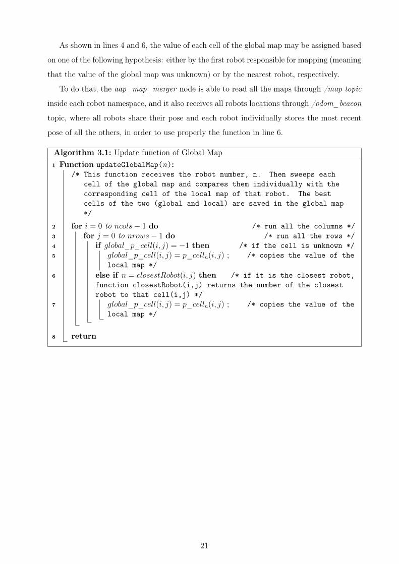
As shown in lines 4 and 6, the value of each cell of the global map may be assigned based
on one of the following hypothesis: either by the first robot responsible for mapping (meaning
that the value of the global map was unknown) or by the nearest robot, respectively.
To do that, the aap_map_merger node is able to read all the maps through /map topic
inside each robot namespace, and it also receives all robots locations through /odom_beacon
topic, where all robots share their pose and each robot individually stores the most recent
pose of all the others, in order to use properly the function in line 6.
Algorithm 3.1: Update function of Global Map1 Function updateGlobalMap(n):
/* This function receives the robot number, n. Then sweeps eachcell of the global map and compares them individually with thecorresponding cell of the local map of that robot. The bestcells of the two (global and local) are saved in the global map*/
2 for i = 0 to ncols− 1 do /* run all the columns */3 for j = 0 to nrows− 1 do /* run all the rows */4 if global_p_cell(i, j) = −1 then /* if the cell is unknown */5 global_p_cell(i, j) = p_celln(i, j) ; /* copies the value of the
local map */6 else if n = closestRobot(i, j) then /* if it is the closest robot,
function closestRobot(i,j) returns the number of the closestrobot to that cell(i,j) */
7 global_p_cell(i, j) = p_celln(i, j) ; /* copies the value of thelocal map */
8 return
21

(a) Local robot_0 map.
(b) Local robot_1 map.
(c) Global map.
Figure 3.2: Map merging scenario in the beginning of a multi-robot map operation. Theaap_map_merger node reads from each robot /map topic (a) and (b) and combines theminto the global map (c).
3.5 Localization
When mapping a real environment the robot’s sensors have a high sensitivity to errors,
generating faulty maps. To overcome this situation it may be necessary to resort to the
application of SLAM, which allows to obtain a map as close as possible to reality while
being able to establish the location of the robot ate the same time.
In a simulation the exact location of the robot can be provided, making the application
of any method for SLAM unnecessary. So, although gmapping (or any other package that
performs SLAM) will be indispensable in real tests, in a simulation it will only introduce an
unwanted extra computational load. Thus, arises the need to create a mapping node to take
advantage of the robot localization provided by the simulator, namely the aap_mapping4
package. The node created by aap_mapping, subscribes four important topics, /scan, /odom,
/global_map and /odom_beacon (topic where each robot publishes its own position).
With the LRF readings and with the current position of the robot the aap_mapping node
has all the data needed to map. The readings are transformed into points in the map and
the probability of occupation is updated following the method of log odds. It is incremented
whenever the distance obtained is less than the laser range and decremented when it is equal
4http://wiki.ros.org/arena/aap_mapping
22

to the range. Between each point obtained, and taking into account the position of the laser,
empty points are generated, being the distance among them equal to the resolution of the
occupancy grid, lowering the probability of occupation.
Analyzing the sequence of images presented in figure 3.3, the map growth with a difference
of 1 second between images can be observed through the application of the method previously
explained.
(a) (b)
(c) (d)
Figure 3.3: Progressive growth of a map using the aap_mapping package.
In a cooperative exploration it becomes indispensable that the mapping node is able
to combine its own map with the global map, using the same method created for the
aap_map_merger. If only a map replacement was made the latest updates of the map
would be lost, hence the need for /global_map and /odom_beacon topics, to enable the
node to apply a similar version to the algorithm 3.1. In this case the occupancy probability
of a cell, in a local map, is only kept if the robot is the closest to that cell, otherwise it will
be replaced by the global map probability.
23

3.6 Frontier Generation Node
The definition of frontier cell (see definition 2.1) is fairly constant in literature, and so
is the method for frontier cells identification. A package was created for the application of
this method, aap_frontiers5, with the additional purpose of generating a binarized version
of the map, in which the present cells may have one of the following values:
unknown cell: f_celln(i, j) = −1, which means that p_celln(i, j) = −1;
free cell: f_celln(i, j) = 0, which means that 0 ≥ p_celln(i, j) > 0.5;
occupied cell: f_celln(i, j) = 1, which means that 0.5 ≥ p_celln(i, j) ≥ 1;
frontier cell: f_celln(i, j) = 2;
inaccessible cell: f_celln(i, j) = 3.
It was understood that an binarized map with identified frontier cells (see figure 3.4b)
identified was more beneficial than a vector containing only the frontiers indexes, since in
explorations both the map and the frontiers are necessary.
Thus, it is possible to transmit the desired information (ROS occupancy grid) through
/frontiers topic using a binarized map, contrary to what occurs when resorting to the use
of the vector.
To increase process efficiency, the algorithm 3.2 generates a binary version of the map
(e.g. line 10 to 13), while identifying the frontiers(e.g. line 10 to 13). Each occupied cell
in the normal map (not binarized) will generate a region in the binarized map centered
on it (e.g. algorithm 3.2 line 13), with a radius slightly higher than the robot radius (e.g.
algorithm 3.4 - line 2), where all cells will be marked as occupied. Thus, all free cells can be
considered as passable, making this a very useful feature for the calculation of cost maps.
Keeping in mind one of the main objectives, the identification of frontier cells, the al-
gorithm 3.2 resorts to the algorithm 3.3 in order to identify if an unknown cell is in fact a
frontier (revise the definition 2.1).
5http://wiki.ros.org/arena/aap_frontiers
24

In figure 3.4 the result of one iteration of algorithm 3.2 can be visualized.
(a) Robot local map. (b) Robot frontier map
Figure 3.4: An example of a frontier map generated from a local map of a robot. Theoccupied cells are represented in black on the map (a) and purple on the map (b).Thefrontier cells are highlighted in yellow.
On the left image:
unknown cell: grey, p_celln(i, j) = −1;
free cell: white, 0 ≥ p_celln(i, j) > 0.5;
occupied cell: black, 0.5 ≥ p_celln(i, j) ≥ 1.
On the right image:
unknown cell: grey, f_celln(i, j) = −1;
free cell: white, f_celln(i, j) = −0;
occupied cell: black, f_celln(i, j) = 1;
frontier cell: yellow, f_celln(i, j) = 2.
Algorithm 3.2: Update Frontiers Map1 Function updateFrontiersMap():
/* This function identifies the frontiers and generates a binarizedversion of a local map */
2 for i = 0 to ncols− 1 do /* run all the columns */3 for j = 0 to nrows− 1 do /* run all the rows */4 if f_celln(i, j) 6= 3 then /* if it is not an inaccessible cell */5 if p_celln(i, j) = −1 then /* if it is an unknown cell */6 if isFrontier(i, j) = true then /* if it is a frontier cell */7 f_celln(i, j) = 2 ; /* marks as a frontier cell */8 else /* if it is not a frontier */9 f_celln(i, j) = −1 ; /* marks as an unknown cell */
10 else if 0 ≤ p_celln(i, j) < 0.5 then /* if it is more probably afree cell */
11 f_celln(i, j) = 0 ; /* marks as a free cell */
12 else /* if it is more probably an occupied cell */13 inflameObstacles(i, j)
14 return
25

Algorithm 3.3: Frontier identification algorithm1 Function isFrontier(i,j):
/* This function receives the index of an unknown cell and finds outif the cell is a frontier cell */
2 if i− 1 ≤ 0 then imin = 0 else imin = i− 1; /* starting column */3 if i+ 1 ≥ ncols− 1 then imax = ncols− 1 else imax = i+ 1; /* end column */4 if j − 1 ≤ 0 then jmin = 0 else jmin = j − 1; /* starting row */5 if j + 1 ≥ nrows− 1 then jmax = nrows− 1 else jmax = j + 1; /* end row */
6 for i = imin to imax do /* runs 3 columns */7 for j = jmin to jmax do /* runs 3 rows */8 if 0 ≤ p_celln(i, j) ≤ 0.5 then /* if it is a free cell */9 return true ; /* is a frontier */
10 return false ; /* is not a frontier */
Algorithm 3.4: Inflame Obstacles1 Function inflameObstacles(i,j):
/* This function receives the index of an occupied cell and marks itas occupied as well as all cells within x cells from it */
2 x = ceil(robot_radius/resolution) ; /* number of cells, rounded up */
3 if i− x ≤ 0 then imin = 0 else imin = i− x; /* starting column */4 if i+ x ≥ ncols− 1 then imax = ncols− 1 else imax = i+ x; /* end column */5 if j − x ≤ 0 then jmin = 0 else jmin = j − x; /* starting row */6 if j + x ≥ nrows− 1 then jmax = nrows− 1 else jmax = j + x; /* end row */
7 for i = imin to imax do /* runs the columns */8 for j = jmin to jmax do /* runs the rows */9 if 0 ≤ p_celln(i, j) ≤ 0.5 then /* if it is a free cell */
10 f_celln(i, j) = 1 ; /* marks as an occupied cell */
26

3.7 Summary
The need for a simulator to test the created exploration algorithm (see chapter 4) proved
to be essential in the course of this work. ARENA emerged of this need since there is no
specific simulator for frontier-based explorations.This aims to answer all the needs of an
exploration algorithm facilitating the development and experimentation of it, which made
its availability as open-source software imperative.
In the next chapter a description of the frontier-based exploration algorithm will be
made.
27

28

4 CoopExp - Exploration Algorithm
This chapter presents the exploration algorithm which was developed to be compatible
with ARENA and also to overcome the restrictions imposed by the ISR robot fleet and by
network conditions.
As mentioned in chapter 1 it was decided to create a new algorithm that would bring
together the strengths of all the analyzed algorithms. For that purpose the CoopExp package
was developed from the ground up.
The CoopExp package must be launched multiple times in order to have a node per robot
just as other packages of this project. Once launched, the nodes will generate the objectives
of the exploration. These will take into account the position of other robots and the areas
already explored by them, making the exploration of the environment as efficient as possible.
This node requires the following topics:
1. /frontiers, that contains the location of the frontiers and the binarized map of the
environment (updated periodically with the global map);
2. /odom_beacon, which has all the robot’s current position.
With the information provided by these topics the cost and utility for each frontier cell
are calculated and exploration goals are generated based on the final value, which combine
both (see table 4.1). This process can be divided into three stages: the calculation of the
cost, the calculation of utilities and the generation of goals.
Table 4.1: Cell values notation for the costmap value c, utility value u and final explorationvalue v.
Notation Meaningc_celln(i, j) cost value of cell(i, j) of the robot nu_celln(i, j) utility value of cell(i, j) of the robot nv_celln(i, j) final value exploration value of cell(i, j) of the robot n
29

4.1 The Costmap Generation
The algorithm responsible for the calculation of the costmap is based on the Burgard et
al. [5] algorithm. To determine the cost of reaching the current frontier cells an optimal path
from the current position of the robot to all frontier cells was computed. This operation is
based on a deterministic variant of the value iteration, which is a popular dynamic program-
ming algorithm [17]. In this approach, the cost of reaching a cell(i, j) is proportional to its
occupancy value p_celln(i, j). The minimum cost is computed using the following two steps:
Initialization:
All the cells contained in the robot footprint are initialized with 0, all others with ∞;
Update loop:
c_celln(i, j) = min{c_celln(i+ ∆i, j + ∆j) +
√∆i2 + ∆j2 · p_celln(i+ ∆i, j + ∆j)
}∆i,∆j ∈ {−1, 0, 1} and p_celln(i+ ∆i, j+ ∆j) ∈ [0, p_cellmax]
The update loop is repeated until convergence, performing a sweep of all cells in the
costmap always in the same order. This process is very demanding even for small grids.
Tests to support this statement in chapter 5 are shown.
The method mentioned above is computationally very demanding and in a simulation
the computational load will increase proportionally to the number of robots resulting in an
unfeasable implementation of this algorithm.
Due to this problem an evolution of the algorithm was developed that could fill the
costmap more efficiently, thus making it possible to handle the computational load resulting
from the simulation of multiple robots. Taking advantage of the binarized map of the topic
/frontiers, the contribution of the occupation probability in the update loop was removed,
and instead of being initialized at infinity it is initialized at -1 (meaning unknown cost).
30

Initialization:
All the cells contained in the robot footprint are initialized with 0 (minimum cost), all
others with −1 (unknown cost);
Update loop:
if f_celln(i, j) = 1⇒ c_celln(i, j) = −2
else c_celln(i, j) = min{c_celln(i+ ∆i, j + ∆j) +
√∆i2 + ∆j2
}with
with ∆i,∆j ∈ {−1, 0, 1}, c_celln(i+ ∆i, j + ∆j) ≥ 0 and f_celln(i+ ∆i, j + ∆j) 6= 1
A new version of the costmap has to be obtained before the generation of a new goal,
because when the robot changes its position the costmap gets outdated. So, for each version
of the costmap the algorithm 4.1 has to be applied to perform the initialization step that
sets out a neutral cost in the area under the robot (e.g. line 4 and 5).
Algorithm 4.1: Costmap Initialization Function.1 Function initCostmap():
/* This function sweeps all the grid cells of the costmap andinitializes them with the right value */
2 for i = 0 to ncols− 1 do /* runs all the columns */3 for j = 0 to nrows− 1 do /* runs all the rows */
4 if the robot footprint contains cell(i,j) then /* cell(i,j) is thephysical space occupied by one cell in the map */
5 c_celln(i, j) = 0 ; /* 0 is the minimum cost */6 else7 c_celln(i, j) = −1 ; /* -1 represents an unknown value */
8 return
Despite the changes mentioned above the significant gain in efficiency results from the
optimization of the cell sweep, when applying the second step (update loop) of this new
method until its convergence. Algorithm 4.2 has been designed in order to make that spiral
sweep beginning in the robot location (e.g. line 7 to 10 and line 14 and 16).
31

After a first spiral sweep on an empty map only filled with free or unknown cells, a full
costmap is obtained regardless of the location of the robot and unlike the original algorithm,
which means that all the cells in it have a positive cost value. When generating a costmap
from a map with obstacles, unknown cost cells could be maintained, which implies that a
new sweep has to be performed (e.g. line 30). However, the ratio of cells with positive cost
is much higher in a spiral sweep than in a common sweep.
Algorithm 4.2: Costmap Update Function.1 Function updateCostmap(i, j):
/* i and j define the starting point for the algorithm */
2 iterations = max[nrows, ncols];3 direction = [counterclockwise, clockwise];4 side = [bottom, right, top, left];5 squareside = 1;6 incomplete = false;
7 for n = 0 to iterations do8 foreach direction do9 foreach side do
10 for s = 0 to squareside do
11 if i >= 0 and i < ncols and j ≥ 0 and j < nrows) then12 c_celln(i, j) = minCost(i, j) ;13 if c_celln(i, j) = −1 then14 incomplete = true ;
15 if counterclockwise then16 if bottom then i+ +;17 else if right then j + +;18 else if top then i−−;19 else if left then j −−;20 else if clockwise then21 if bottom then j + +;22 else if right then i+ +;23 else if top then j −−;24 else if left then i−−;
25 i−−,j −− ; /* goes to the starting point of the next iteration */26 squareside+ = 2; /* with the square side increased */
27 if incomplete = true then28 [i, j] = findNextStartingPoint();29 if i 6= −1 then30 updateCostmap(i, j);
31 return
32

Algorithm 4.3: Find Next Starting Point.1 Function findNextStartingPoint():
/* This function sweeps all the grid cells of the costmap in searchof a costmap cell with the value of -1 and that is surrounded bya cell with a cost bigger than zero */
2 minV alue =∞;3 valid = false;
4 for i = 0 to ncols− 1 do /* runs all the columns */5 for j = 0 to nrows− 1 do /* runs all the rows */
6 if c_celln(i, j) = −1 then
7 costtemp = minCost(i, j);
8 if 0 ≤ costtemp < minV alue then9 minV alue = costtemp ;
10 startPointi = i ;11 startPointj = j ;12 valid = true;
13 if not valid then14 return −1,0 ;
15 return startPointi,startPointj ;
Whenever at least one cell with an unknown cost remains in the costmap, the algorithm
4.2 is able to detect it (e.g. algorithm 4.2 line 14) and resorts to algorithm 4.3 (e.g. algorithm
4.2 line 28) to identify a point in the unknown area so that the algorithm 4.2 starts a new
spiral sweep centered on it (e.g. algorithm 4.2 line 30). This way it is much more effective.
Once algorithm 4.2 starts in an unknown cost cell it is able to calculate more values for the
remaining unknown costmap cells.
When sweeping the costmap, the c_celln(i, j) is given by the application of algorithm 4.4
(e.g. algorithm 4.2 line 12). This algorithm analyses a set of cells composed by that cell(i, j)
and the eight cells that surround it, then the minimum cost is selected (e.g. algorithm 4.4
line 17), according to the second step of the costmap generation.
33

Algorithm 4.4: Minimum Cost Function.1 Function minCost(i, j):
/* This function will return the minimum cost of the set of cellscomposed by the cell(i,j) and the eight cells that surround it */
2 if f_celln(i, j) = 1 then /* cell is occupied */3 return −2 ; /* -2 represents an infinity value due to an occupied
cell */
4 minV alue =∞;5 icenter = i;6 jcenter = j;
7 if i− 1 ≤ 0 then imin = 0 else imin = i− 1; /* starting column */8 if i+ 1 ≥ ncols− 1 then imax = ncols− 1 else imax = i+ 1; /* end column */9 if j − 1 ≤ 0 then jmin = 0 else jmin = j − 1; /* starting row */
10 if j + 1 ≥ nrows− 1 then jmax = nrows− 1 else jmax = j + 1; /* end row */
11 for i = imin to imax do /* runs 3 columns */12 for j = jmin to jmax do /* runs 3 rows */
13 if f_celln(i, j) 6= 1 then /* is not occupied */14 disttemp = sqrt(((icenter− i)∗ resolution)2 +((jcenter− j)∗ resolution)2));15 costtemp = c_celln(i, j) + disttemp;16 if 0 ≤ costtemp < minV alue then /* new minimum */17 minV alue = costtemp ; /* saves the new minimum */
18 if minV alue =∞ then /* in this case the minimum value keepsunchanged so the cost of reaching that cell is still infinity */
19 return −1 ;
/* if the algorithm reaches this point then the minValue has to bevalid */
20 return minV alue
34

In figure 4.1b the costmap generated based on the map of figure 4.1a can be seen. The
cost is set in shades of gray for an easy analysis, where white means a zero cost and black a
maximum cost.
(a) Environment. (b) Costmap.
Figure 4.1: An example of a costmap (b) generated based on map (a) by the spiral sweepingalgorithm. The costmap values are identified in shades of gray, the higher the shade thehigher the cost.
4.1.1 Classification of Costmap Algorithms
In order to obtain the classification of an algorithm according to the rating of the Big
O Notation [8] , the worst case scenario has to be considered. In terms of the calculation
of costs, the worst case scenario is the existence of a u-turn (forced reversal) since for each
required inversion there is a 1 unit increase in the complexity of the map.
Figure 4.2: An illustration of a map with 8 u-turns (forced reversal).
Figure 4.2 allows to obtain a better understanding of this concept. The map shown
35

has a complexity (complexity c) which is proportional to the number of inversions (u-turns)
required to reach the point B starting from A, this being the worst case scenario.
Therefore,
c = 1 + u, (4.1)
being u, the number of u-turns in the map. Once understood this concept can be trans-
posed to the classification of the algorithms.
Assuming a square map of n cells with complexity c, the classification algorithms would
be:
Standard sweeping: O(cn1.5), quadric algorithm
Spiral sweeping: O(2cn), linear algorithm
Taking into account a map with 400 by 400 cells (n = 160000) and c = 9, the numbers
of iterations needed to complete the costmap in the worst situation are:
Standard sweeping: 9 ∗ 1600001.5 = 576000000 iterations
Spiral sweeping: 9 ∗ 2 ∗ 160000 = 2880000 iterations
0 0.2 0.4 0.6 0.8 1 1.2 1.4 1.6 1.8 2
·105
0
2
4
6
8·108
n
iterations
O(cn1.5)O(2cn)
Figure 4.3: A graphical comparison between the two Big O classifications, O(cn1.5) andO(2cn). The graph shows the growth of the number of iterations in function of n, for acomplexity c = 9.
Thus, through the analysis of the above results it can be concluded that to calculate
the full costmap 200 fewer iterations in a spiral sweeping are required, when compared to a
standard sweeping. This difference is increasingly noticeable the larger the n, as can be seen
in the graph of figure 4.3.
36
4.2 The Utility of a Frontier Cell
In this work the utility is calculated only for the frontier cells before generating any
goal for the exploration, which demonstrates a lower computational effort compared to the
costmap generation which needs to examine all map cells1. The utility is defined by two
parameters, namely:
1. Number of nearby frontiers, that contains the location of the frontiers and the
binarized map of the environment (updated periodically with the global map);
2. Minimum distance to other robots, which has all the robot’s current position.
Which then are combined into the following equation:
u_celln(i, j) = α ∗ numberOfNearbyFrontiers(i, j)+
β ∗minDistOtherRobots(i, j) (4.2)
The gains α and β allow to adjust easily the weight of each parameter.
For a better understanding of this issue the following concepts, number of nearby frontiers
and minimum distance to other robots, will be described in the following sections as algorithm
4.5 and 4.6, respectively.
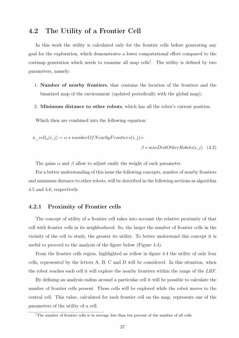
4.2.1 Proximity of Frontier cells
The concept of utility of a frontier cell takes into account the relative proximity of that
cell with frontier cells in its neighborhood. So, the larger the number of frontier cells in the
vicinity of the cell to study, the greater its utility. To better understand this concept it is
useful to proceed to the analysis of the figure below (Figure 4.4).
From the frontier cells region, highlighted as yellow in figure 4.4 the utility of only four
cells, represented by the letters A, B, C and D will be considered. In this situation, when
the robot reaches each cell it will explore the nearby frontiers within the range of the LRF.
By defining an analysis radius around a particular cell it will be possible to calculate the
number of frontier cells present. Those cells will be explored while the robot moves to the
central cell. This value, calculated for each frontier cell on the map, represents one of the
parameters of the utility of a cell.
1The number of frontier cells is in average less than ten percent of the number of all cells
37

Figure 4.4: Frontier cells line (yellow) in a wide area. Points A, B, C and D are frontier cells.The distance from any of the points to the robot and also from A to D is equal to LRFrange.
It is desired to have a analysis area defined by a circular shape with a perimeter equal
to the LRFrange, so the analysis radius is:
Rmeters = 0.5 ∗ LRFrange. (4.3)
Being LRFrange equal to the distance from A to D, it can be concluded that the number
of frontier cells reached from the positions A and D (edges of the frontier cell region) are
lower compared to the positions B and C. Therefore, its utility is reduced.
For the sake of simplicity, to obtain the number of frontier cells a radius in cells is used
rather a radius in meters, thus:
Rcells = ceil
(0.5 ∗ LRFrange
mapresolution
)(4.4)
However, this analysis radius can create a problem whenever it becomes necessary to
decide which frontier cell to explore within a hall (see figure 4.5).
Whenever a hall has a width equal or inferior to half the range of the LRF, the utility
of any frontier cell present will not be differentiated. Through the analysis of figure 4.5 it is
possible to infer that the number of frontier cells in the neighborhood of is points A, B, or C
is the same, since the neighborhood radius is defined as being half the sensor range (range
4m, 2m half). Since the longest distance between two cells, A and C, is smaller than this
radius (1.5m), it could be concluded that the number of frontier cells in the neighborhood
of any of these points is the same.
38

Figure 4.5: Frontier cells line (yellow) in a hall. Points A, B, and C are frontier cells. Thedistance from any of the points to the robot is equal to LRFrange.
To solve this problem a radius which takes into account the minimum width is set thus
allowing an easy and safe passage of the robot through the halls of the map. So,
Dmin = 2 ∗ diameterrobot. (4.5)
If there are more narrow hallways than this distance (Dmin), the algorithm may show
abnormal behaviors.
Thus, the radius of the cells should be:
Rcells = ceil
(0.5 ∗Dmin
mapresolution
)= ceil
(diameterrobotmapresolution
)= ceil
(2 ∗ radiusrobotmapresolution
)(4.6)
Concluding, and taking into account the aforementioned parameter, the frontier cells
with greater utility are cells B and C of figure 4.4 and B of figure 4.5.
The algorithm 4.5 listed above, represents the method used to calculate the number of
frontier cells ( e.g. line 10 and 11) in the neighborhood of a particular frontier cell ( e.g. line
2 to 9).
4.2.2 Minimum Distance to Other Robots
A cooperative exploration could lead to the simultaneous mapping of the same area or the
areas already explored in situations where robots are in close proximity, which significantly
reduces the efficiency of the exploration. To overcome this situation, adding a repulsion
factor between the robots that would determine an increase of the utility of the frontier cells
become necessary.
39

Algorithm 4.5: Number of nearby frontiers.1 Function numberOfNearbyFrontiers(i,j):
/* This function receives the index of a frontier cell and countsthe number of frontiers within x cells from it */
2 x = ceil(2 ∗ robot_radius/resolution) ; /* number of cells, rounded up */
3 counter = 0;
4 if i− x ≤ 0 then imin = 0 else imin = i− x; /* starting column */5 if i+ x ≥ ncols− 1 then imax = ncols− 1 else imax = i+ x; /* end column */6 if j − x ≤ 0 then jmin = 0 else jmin = j − x; /* starting row */7 if j + x ≥ nrows− 1 then jmax = nrows− 1 else jmax = j + x; /* end row */
8 for i = imin to imax do /* runs the columns */9 for j = jmin to jmax do /* runs the rows */
10 if f_celln(i, j) = 2 then /* if it is a frontier cell */11 counter + + ; /* increments the counter */
12 return counter
Each robot assigns a value, corresponding to this incrementation, to all frontier cells of
the local map, resorting to algorithm 4.6. The higher the minimum distance (e.g line 7)
between a particular frontier cell and other robots, the higher their usefulness.
Algorithm 4.6: Minimum distance to other robots.1 Function minDistOtherRobots(i,j):
/* This function receives the index of a frontier cell and returnsthe distance of the closest robot to that cell excluding therobots which is using this algorithm */
2 mindistance =∞ ;
3 for k = 0 to numberOfRobots− 1 do /* runs one time for each robot */4 if k 6= robotnumber then /* is not the distance for the robot which
is using this algorithm */5 distance = sqrt((x_robotk − x_cell(i, j))2 + (y_roboti − y_cell(i, j))2) ;6 if distance < mindistance then /* new minimum distance */7 mindistance = distance ; /* saves the new minimum */
8 return mindistance
In order to achieve a better understanding of this theme figure 4.6 in which the influence
of this parameter is noticeable should be examined.
When it is necessary to choose which of the frontier cells, A or B, is more useful to
be explored by robotleft, it is important to consider different factors to achieve the best
exploration goal. If only the cost of the robot movement was considered, the selected cell
would certainly be frontier cell B, since the distance from robotleft to A is 2,5 m and while B
40

Figure 4.6: An example of a proximity case between two robots. The frontier cells are inyellow and in purple are the obstacles. Two frontier cells (A and B) are highlighted in redin order to demonstrate which cell would be chosen for exploration.
is only 1m away. However, when taking into account the value of the minimum distance to
other robots, in this case the distance of the cells A and B in relation to robotright, the choice
of cell to explore would fall on the frontier cell A. Thus, although the B cell is the closest
to robotleft it is also closer to robotright, which makes their exploration less effective. The
difference of 1.5 meter in the cost of robotleft achieving A in relation to B is compensated
by the higher distance of robotright to A, this being the frontier cell selected.
4.3 Goal Generation
Having specified the costs and utilities of all frontier cells, the exploration node will
select the frontier with the highest value as the next objective of exploration. This values
are obtained from the following equation:
value_celln(i, j) = u_cellm(i, j)− c_celln(i, j) (4.7)
Throughout the application of this equation the index of the cell with the maximum
value, obtained so far, is kept. Thus, when all frontier cells have an assigned value the index
of the absolute maximum is known. A simple conversion to geographic coordinates is applied
to the index, and these are later introduced in the topic /goal. This goal will be received
in the robot’s move_base node, steering it if possible to that cell. Whenever move_base
is unable to identify a safe path to the desired position, the algorithm marks this cell as
inaccessible, depreciating its value in future iterations.
41

When all the frontier cells were explored or marked as inaccessible, the exploration is
taken as completed.
4.4 Summary
In this chapter the CoopExp, exploration algorithm was presented.
This package can be divided into three areas: the generation of the cost map; the gener-
ation of utility for the frontiers; and the generation of exploration goals. It is worth pointing
out that this package is available online at wiki-ros web page, as referred to in the beginning
of the chapter.
In the next chapter an exposition of the validation tests of ARENA and CoopExp will be
done.
42

5 Validation and Results
In order to evaluate and validate the performance of the system, multi-robot exploration
tests were performed both in multiple simulated environments and in a real-world scenario.
With the purpose of illustrating each system’s performance, two distinct stages took
place: one to test ARENA performance and scalabity (section 5.1) and another to validate
the CoopExp application (section 5.2).
5.1 ARENA Performance
To test the performance of ARENA became necessary the use of multiple robots, to a
maximum of 16 robots. As expected, when simulations are performed with 16 robots, the
use of a computer with greater processing capacity, namely a Lenovo with an Intel i7 Quad-
Core processor became necessary. However, even with the help of computers equipped for
the purpose, it was impossible to perform such simulations (16 robots) in real time. To work
around this situation, the simulator clock speed was decreased to a 0.1 factor, where every
second corresponds to 0.1 seconds of simulated time required for the simulation.
On the other hand with 8 robots the computer is capable of performing the simulation
in real time.
After this conclusion it was decided to perform the test with 16 robots only as a proof of
concept, since the reduction of the clock speed required in this experiment would reduce the
Central Processing Unit (CPU) load, which is the variable used to evaluate the performance
of the simulator. In figure 5.1 the environment and map and of this simulation can be viewed.
The remaining tests were done in real time with a maximum of 8 robots, in which the
CPU load has been analyzed and summarized in the graph present in figure 5.2 in accordance
with the number of robots. In this graph it is easy to acknowledge the growing burden of
adding robots to the simulation.
43

(a) Simulated environment showing the pathof the robots (in blue).
(b) Frontier map of the simulation after 10seconds.
Figure 5.1: An example of a simulation with 16 robots using ARENA.
0 2 4 6 8 1020
40
60
80
100
Number of robots
CPU
load
(%)
Figure 5.2: A graphical illustration of a CPU load in function of the number of robots in aQuad-Core computer.
Tests were also carried out in a Dual-Core computer (graph of figure 5.3) to verify its
viability on computers with less processing load. As expected, the simulation capability was
limited to 4 robots in real time and 8 robots with reduced clock speed. These results show
that the scalability of the simulator is real, but it is very limited by the processing capacity
of the machine that runs the simulator.
44

2 3 4 540
60
80
100
Number of robots
CPU
load
(%)
Figure 5.3: A graphical illustration of a CPU load in function of the number of robots in aDual-Core computer.
5.2 CoopExp Experimentation
5.2.1 Gains Calibration
While developing the exploration algorithm, the ability to adapt to different situations
was assigned resorting to the implementation of gains (α and β).
In the equation 4.2 from the chapter 4, the alpha and beta, allow changing the influence
of utility parameters in exploration, namely:
• Number of nearby frontiers;
• Minimum distance to other robots.
Default gains allocated to the algorithm have been achieved through an initial calibration,
which is described in this chapter in order to facilitate future calibrations.
During the calibration several simulations were performed using equal conditions: virtual
environment (figure 5.4) of 20 by 20 meters and a resolution of 5 centimeters; two robots
with a radius of 0.2 meters.
This environment was selected taking into account two objectives: increase the number
of situations in which frontier cells have the same cost despite being in different areas; to
allow the geometric distance between a robot and a frontier cell to have approximately the
same value of the cost of reaching it, due to lack of closed areas.
45

Figure 5.4: Grid map for gains calibration.
Alpha Calibration
Before calibrating the gain alpha it is important to get aware of its influence in the
calculation of utility (equation 4.2 - Chapter 4). Remembering the latter equation and
admitting β = 0, the utility value is increment by one unit for each frontier cell in the
vicinity of the cell(i, j).
Given that the map boundaries are typically continuous and slightly curved, it can be
assumed that the average number of returned frontiers cells is equal to doubling the radius
in cells in the neighborhood analyzed by the algorithm 4.5.
nfrontiers = 2 ∗ ceil(
2 ∗ radiusrobotmapresolution
)= 2 ∗ ceil
(2 ∗ 0.2
0.05
)== 2 ∗ ceil
(0.4
0.05
)= 16 (5.1)
However, an increase of 16 units in the utility of a frontier cell is exaggerated, since this
value only wants to differentiate frontier cells close to each other. Thus, it was selected as
the starting point α = 0.1 to obtain an enhancement equal to 1.6 in a normal situation,
which is an acceptable value. As for the calibration, variations of the starting point alpha
were made with intervals of ±0.025 to it. For each variation ten explorations were performed
and the medium time for each had a variation according to the graph in figure 5.5.
By analyzing the graph it is easily observable that the exploration time is minimal when
α = 0.125, which is the default value assigned to the gain alpha.
Beta Calibration
Contrary to the alpha, the beta gain aims at distinguishing any cell regardless of its
position, thus being chosen as the starting point for beta calibration 1.0.
The beta calibration was performed in a variation range of ±0.1 and the average ex-
46

5 · 10−2 0.1 0.15 0.2
125
130
135
140
145
150
“minimum 0.125”
α
averag
eexplorationtime(s)
Figure 5.5: A graphical illustration of the results obtained in each set of the alpha calibration.
ploration times varied according to the graph in figure 5.6, again for each gain value 10
experiments were conducted.
0.6 0.8 1 1.2
125
130
135
140
145
150
“minimum 0.8”
β
averag
eexplorationtime(s)
Figure 5.6: A graphical illustration of the results obtained in each set of the beta calibration.
Through the analysis of the graphic it can be concluded that the exploration time is
minimal when beta is equal to 0.8 (default value).
5.2.2 Efficiency in Simulated Environments
To test the efficiency of the exploration algorithm experiments with multiple robots were
performed. Ten sets of experiments with up to 8 robots in 4 different environments, namely
the ones in figure 5.7.
From the relationship between the average exploration time of each set of experiments
and the number of robots used, the graphs of figures 5.8 to were created. By doubling the
47

(a) Grid. (b) Big room. (c) Triple u-turn. (d) Office floor.
Figure 5.7: Different environments for simulation with multiple robots.
number of robots used, the time of exploration should have been halved. However, some of
these maps have certain specificities that do not allow to assert this statement.
When dealing with a map that presents a division with one access zone an increase in
the exploration time is expected since to explore this area the robot has to enter and exit
through the same location, opposed to what would occur if the map had multiple zones of
access. This increase in the exploration time should be mitigated when the robot number
is equal to or higher than the number of divisions on the map [40]. That fact could be
visualized in the graph line (figure 5.8) corresponding to environment of figure 5.7d.
2 3 4 5 6 7 825
50
75
100
125
150
175
number of robots
averageexplorationtime(s) grid
big roomtriple u-turnoffice floor
Figure 5.8: A graphical illustration of multiple experiences performed in four different sim-ulated environments using ARENA.
The efficiency of individual exploration was calculated with reference to the exploration
time with two robots. For example, after exploring a map with two robots in 120 seconds,
it was concluded that to have an efficiency of 1.0 (expected) the exploration should be
accomplished with 4 robots in 60 seconds and 8 robots 30 in seconds.
If the exploration is performed with 4 robots, but within a period of 90 seconds, the
48

efficiency will be lowered to 0.(6) = 60/90. On the other hand, there is an increase in
efficiency if the exploration time is reduced, for example in 45 seconds the efficiency is
1.(3) = 60/45.
Figure 5.9: A graphical illustration of the experience performed in the Grid environment.
Figure 5.10: A graphical illustration of the experience performed in the Big room environ-ment.
In the graphics of figures 5.9 and 5.10, the exploration time did not decrease constantly
with the growth of the number of robots, as expected. However, this reduction does not
reflect an efficiency of 1.0, but is slightly lower, between 0.6 and 0.9, due to the inevitable
mapping of some areas.
On the graphic of figure 5.11, the exploration times demonstrated the lowest efficiencies in
all scenarios. The efficiency of 0.35 for 8 robots was the lowest recorded. The team becomes
less efficient with the addition of more agents, since this environment has little diversity of
paths to be taken by the multiple robots, benefiting simultaneously mapping situations.
49

Figure 5.11: A graphical illustration of the experience performed in the Triple u-turn envi-ronment.
Figure 5.12: A graphical illustration of the experience performed in the Office floor environ-ment.
The graphic of figure 5.12 shows interesting results since exploration times are stagnated
in four of the set of tests. Nevertheless the results have the highest efficiencies in the tests
with 4 robots (almost 1.0 of efficiency) and 8 robots (0.82 of efficiency). In this environment
the robots are faced with multiple divisions with a single access, which leads to a remapping
of the area and consequent reduction in exploration efficiency, since the robot has to enter
and exit through the same place. When the robot number is increased to a value higher
than the number of divisions, the robot team can perform a simultaneous exploration of
all the different areas, without having to leave those divisions, leading to the end of the
exploration and thus avoiding remapping on the way back, therefore increasing the efficiency
of the exploration
50

It can be concluded, based on the results achieved in the simulation, the application
feasibility of this algorithm.
5.2.3 Real-World Validation
The final validation of this work was performed in the very end in a real world multi-robot
exploration. In order to do that many real-world issues were taken into account: batteries
must be charged, wireless networks configured, several computers had to be prepared, etc.
Figure 5.13: A small experience set up for real world validation in ISR.
After the environment visible in figure 5.13 was set, the tests were started and instantly
the biggest handicaps of any real exploration were identified, namely the mapping of the
environment and the wireless network. Due to maps errors many trials were made and on
behalf of the wireless network lag, both the exploration and map merger frequency were
reduced. After these modification the exploration was complete successfully in 30 seconds
with 2 robots, although with a significant number of mapping errors as expected.
The same result was then achieved in a few less seconds in simulations with the same
conditions. In figure 5.14a and 5.14b the resultant maps of the real and simulated experiment
can be seen, respectively.
51

(a) Real environment. (b) Simulated environment.
Figure 5.14: An illustration of the frontiers map resulting of both the real and simulatedexplorations.
5.3 Summary
This chapter describes the testing stage of ARENA and CoopExp packages in order to
validate their applicability.
The performance of the ARENA package was tested, and demonstrated in a simula-
tion capacity of 16 robots.This result is extremely important in terms of the computational
requirement of exploration algorithms.
Tests were also carried out for CoopExp efficiency using a variable number of robot
teams in different virtual environments. As a final validation of the package a test in a real
environment was performed.
In the next chapter a brief analysis about the accomplished work as well as an exploration
of possible future works will be done.
52

6 Conclusion
Any dividable system can benefit from the capacities of cooperation, space division,
reliability and robustness of a team of robots. It is logical that all this will have its costs.
Increased complexity, agents maintenance and very strict network conditions have been some
of the factors that prevent the use of the existing potential of a MRS.
This dissertation addresses the issue of cooperation in a MRS in the context of exploration
of territories. As the word suggests, cooperation implies an action: to work together or
collaborate to achieve the same goal, which is the intended purpose. Each robot must
cooperate with other team mates, being assured that each of these will have a satisfactory
and consistent level of knowledge in order to achieve the objective of the proposed mission.
The above frame of reference oversees the application of this system in various applica-
tions, for example in the fields of robotics, army, government and private security, among
others.
At the beginning of this project the testing and implementation of a method capable
of performing a cooperative exploration was proposed and, as a result, a ROS package
compatible with the Pioneer 3-DX, was developed. Although several methods can be found
in the literature, none has been explicitly developed with this premise. This fact prompted
the development of a new operating algorithm, the CoopExp.
The CoopExp was built to work in a decentralized way. This characteristic provides a
resistance to both failures of individual robots as well as in the communication network
without affecting the functioning of the system.
This package offers several potentialities. It has the capacity of both calculating the
cost of reaching a cell using the spiral sweep and the global value of a new exploration goal
with the exchange of information between robots. Furthermore, it is able to answer the
question regarding the exploration process, that is, where the robot should move within the
environment, taking into account the full knowledge of the MRS.
Given the need to test the exploration algorithm, adding a new objective, the creation
53

of ARENA, became necessary.
In order to allow a larger scale simulation three packages were created: the aap_mapmerger,
aap_mapping and aap_frontier. Without these the maximum number of 16 robots in a sim-
ulation would never have been achieved. The features of the different packages are the
combination maps optimized for the simulation which respectively map the use of a perfect
location and identify frontiers.
This work was concluded with a set of experiments that displayed what was intended:
namely, a drastic reduction of the exploration time as a result of cooperation in teams with
different sizes.
The results were very encouraging and are a motivation to continue research and progress
in this area.
The final contributions of this thesis were the CoopExp and ARENA packages.
CoopExp - exploration algorithm that include:
• a new vision on utility of frontier cells;
• an improved costmap generation algorithm based on a spiral sweep of the map.
ARENA - the simulator with:
• a merger package optimized for simulation;
• a mapping package optimized for simulation;
• a frontier identification package.
6.1 Future Work
Whenever a new project emerges, all the effort and dedication go into its development
with the aim of achieving the best possible results. However, there are always different
aspects to be developed, considering an improvement in its functionality and possible future
applications.
Therefore, the aim of this section is to refer and discuss some of these improvements.
In CoopExp package it would be interesting to implement an approach to take advantage
of different features and characteristics of a team of robots. When new parameters are added
54

to calculate the utility it would be possible to distinguish the environmental areas that would
benefit from the different functionalities of each robot. For example, it would be beneficial to
have one or more robots equipped with a long-range sonar capable of mapping larger areas
in the team, or even a robot with a robotic arm capable of diverting path obstacles.
With regard to the ARENA, obtaining the global map is performed through the complete
analysis of local maps, which entails an increase in the number of cells to analyze. This
number could be reduced if only a partial area of the local map defined by the maximum
displacement of the robot between two iterations of the combination of maps was considered.
On the other hand, in order to facilitate the analysis of frontier cells, they could be grouped
into regions, thus reducing the number of calculations necessary for obtaining the exploration
utilities.That is, the process of analyzing a map with thousands of frontier cells would be
faster and more efficient if the cells were combined into a few dozen regions.
The simulation tests show that the most noticeable handicap was the path planning
package, the move_base, which occasionally does not obtain a new path and consequently
makes the robot stand still. Given that to generate a trajectory requires a cost map, a
new trajectory planning package using the algorithm developed in this dissertation could be
developed.
55

56

7 Bibliography
[1] Multi-robot exploration under the constraints of wireless networking, author=Rooker,
Martijn N and Birk, Andreas. Control Engineering Practice, 15(4):435–445, 2007.
[2] Torsten Andre and Christian Bettstetter. Collaboration in Multi-Robot Exploration:
To Meet or not to Meet? Journal of Intelligent & Robotic Systems, pages 1–13, 2015.
[3] Mihai Andries and François Charpillet. Multi-robot taboo-list exploration of unknown
structured environments. In Intelligent Robots and Systems (IROS), 2015 IEEE/RSJ
International Conference on, pages 5195–5201. IEEE, 2015.
[4] Hajime Aoyama, Kazuyoshi Ishikawa, Junya Seki, Mitsuo Okamura, Saori Ishimura, and
Yuichi Satsumi. Development of mine detection robot system. International Journal of
Advanced Robotic Systems, 4(2):229–236, 2007.
[5] Wolfram Burgard, Mark Moors, Cyrill Stachniss, and Frank E Schneider. Coordinated
multi-robot exploration. Robotics, IEEE Transactions on, 21(3):376–386, 2005.
[6] Chih-Fu Chang and Ching-Chih Tsai. Cooperative exploration of networked multi-
robot systems using minimal information entropy. In Networking, Sensing and Control
(ICNSC), 2015 IEEE 12th International Conference on, pages 122–127. IEEE, 2015.
[7] Rafael Gonçalves Colares. The Next Frontier : Combining Information Gain and Dis-
tance Cost for Decentralized Multi-Robot Exploration. In Proc. of 31st ACM Sympo-
sium on Applied Computing (SAC 2016), Pisa, Italy, pages 268–274, 2016.
[8] Thomas H Cormen, Charles E Leiserson, Ronald L Rivest, and Clifford Stein. Intro-
duction to algorithms second edition, 2001.
[9] Edson Prestes e Silva, Paulo M Engel, Marcelo Trevisan, and Marco AP Idiart. Explo-
ration method using harmonic functions. Robotics and Autonomous Systems, 40(1):25–
42, 2002.
57

[10] Eitan Marder Eppstein. Move Base path planning ROS package. URL: http://wiki.
ros.org/move_base [cited 06-08-2016].
[11] Waqar Farooq, Nehal Butt, Sameed Shukat, Nouman Ali Baig, and Sheikh Muhammad
Ahmed. Wirelessly Controlled Mines Detection Robot. In 2016 International Conference
on Intelligent Systems Engineering (ICISE), pages 55–62. IEEE, 2016.
[12] Antonio Franchi, Luigi Freda, Giuseppe Oriolo, and Marilena Vendittelli. A randomized
strategy for cooperative robot exploration. In Proceedings 2007 IEEE International
Conference on Robotics and Automation, pages 768–774. IEEE, 2007.
[13] Antonio Franchi, Luigi Freda, Giuseppe Oriolo, and Marilena Vendittelli. The sensor-
based random graph method for cooperative robot exploration. IEEE/ASME Transac-
tions on Mechatronics, 14(2):163–175, 2009.
[14] Christopher M Gifford, Russell Webb, James Bley, Daniel Leung, Mark Calnon, Joe
Makarewicz, Bryan Banz, and Arvin Agah. Low-cost multi-robot exploration and map-
ping. In Technologies for Practical Robot Applications, 2008. TePRA 2008. IEEE In-
ternational Conference on, pages 74–79. IEEE, 2008.
[15] Giorgio Grisetti, Cyrill Stachniss, and Wolfram Burgard. Gmapping, a highly efficient
Rao-Blackwellized particle filer to learn grid maps from laser range data. URL: http:
//openslam.org/gmapping.html [cited 06-08-2016].
[16] Dave Hershberger, David Gossow, and Josh Faust. RViz, 3D visualization tool for ROS.
URL: http://wiki.ros.org/rviz [cited 06-08-2016].
[17] Ronald A Howard. Dynamic Programming and Markov Processes.. 1960.
[18] Joseph L Jones, Newton E Mack, David M Nugent, and Paul E Sandin. Autonomous
floor-cleaning robot, May 26 2015. US Patent 9,038,233.
[19] Matan Keidar and Gal A Kaminka. Efficient frontier detection for robot exploration.
The International Journal of Robotics Research, page 0278364913494911, 2013.
[20] Kurt Konolige, Dieter Fox, Benson Limketkai, Jonathan Ko, and Benjamin Stewart.
Map merging for distributed robot navigation. In IROS, pages 212–217, 2003.
[21] Maria Teresa Lazaro, Lina María Paz, Pedro Pinies, Jose A Castellanos, and Gior-
gio Grisetti. Multi-robot SLAM using condensed measurements. In Intelligent Robots
58

and Systems (IROS), 2013 IEEE/RSJ International Conference on, pages=1069–1076.
IEEE, 2013.
[22] Yugang Liu and Goldie Nejat. Robotic urban search and rescue: A survey from the
control perspective. Journal of Intelligent & Robotic Systems, 72(2):147–165, 2013.
[23] Gonçalo dos Santos Martins. A Cooperative SLAM Framework with Efficient Informa-
tion Sharing over Mobile Ad Hoc Networks. Master’s thesis, 2014.
[24] Gonçalo S Martins, David Portugal, and Rui P Rocha. A Comparison of General-
Purpose FOSS Compression Techniques for Efficient Communication in Cooperative
Multi-Robot Tasks. In ICINCO (2), pages 136–147, 2014.
[25] Maja J Mataric and Gaurav S Sukhatme. Task-allocation and coordination of multiple
robots for planetary exploration. In In Proceedings of the 10th International Conference
on Advanced Robotics. Citeseer, 2001.
[26] Larry Matthies, Yalin Xiong, R Hogg, David Zhu, A Rankin, Brett Kennedy, Martial
Hebert, R Maclachlan, Chi Won, Tom Frost, et al. A portable, autonomous, urban
reconnaissance robot. Robotics and Autonomous Systems, 40(2):163–172, 2002.
[27] Lynne E Parker. Heterogeneous multi-robot cooperation. Technical report, DTIC Doc-
ument, 1994.
[28] Morgan Quigley, Ken Conley, Brian Gerkey, Josh Faust, Tully Foote, Jeremy Leibs,
Rob Wheeler, and Andrew Y Ng. ROS: an open-source Robot Operating System. In
ICRA workshop on open source software, volume 3, page 5, 2009.
[29] Morgan Quigley, Ken Conley, Brian P. Gerkey, Josh Faust, Tully Foote, Jeremy Leibs,
Rob Wheeler, and Andrew Y. Ng. ROS: an open-source Robot Operating System. In
ICRA Workshop on Open Source Software, 2009. URL: http://wiki.ros.org.
[30] Ioannis Rekleitis, Gregory Dudek, and Evangelos Milios. Multi-robot collaboration for
robust exploration. Annals of Mathematics and Artificial Intelligence, 31(1-4):7–40,
2001.
[31] Rui Rocha, Filipe Ferreira, and Jorge Dias. Multi-robot complete exploration using hill
climbing and topological recovery. In Intelligent Robots and Systems, 2008. IROS 2008.
IEEE/RSJ International Conference on, pages=1884–1889. IEEE, 2008.
59

[32] Rui P Rocha, David Portugal, Micael Couceiro, Filipe Araújo, Paulo Menezes, and
Jorge Lobo. The CHOPIN project: Cooperation between Human and rObotic teams in
catastroPhic INcidents. In Safety, Security, and Rescue Robotics (SSRR), 2013 IEEE
International Symposium on, pages 1–4. IEEE, 2013.
[33] Rui Paulo Pinto da Rocha. Building volumetric maps with cooperative mobile robots
and useful information sharing: a distributed control approach based on enthropy. PhD
thesis, 2006.
[34] Reid Simmons, David Apfelbaum, Wolfram Burgard, Dieter Fox, Mark Moors, Sebas-
tian Thrun, and Håkan Younes. Coordination for multi-robot exploration and mapping.
In AAAI/IAAI, pages 852–858, 2000.
[35] Joan Vallvé and Juan Andrade-Cetto. Mobile robot exploration with potential informa-
tion fields. In Mobile Robots (ECMR), 2013 European Conference on, pages 222–227.
IEEE, 2013.
[36] Richard Vaughan. Massively multi-robot simulation in stage. Swarm Intelligence, 2(2-
4):189–208, 2008.
[37] Eric W. Weisstein. Voronoi Diagram. From MathWorld–A Wolfram Web Resource.
URL: http://mathworld.wolfram.com/VoronoiDiagram.html [cited 08-08-2016].
[38] Ling Wu, Miguel Ángel García García, Domenec Puig Valls, and Albert Solé Ribalta.
Voronoi-based space partitioning for coordinated multi-robot exploration. 2007.
[39] Brian Yamauchi. Frontier-based exploration using multiple robots. In Proceedings of
the second international conference on Autonomous agents, pages 47–53. ACM, 1998.
[40] Zhi Yan, Nicolas Jouandeau, and Arab Ali Cherif. A survey and analysis of multi-robot
coordination. International Journal of Advanced Robotic Systems, 10, 2013.
60