Control and Optimization of Batch Chemical Processes

Dominique Bonvin1,∗ and Gregory Francois2

1 Laboratoire d’Automatique, Ecole Polytechnique Federale de Lausanne

EPFL - Station 9, CH-1015, Lausanne, Switzerland.

2 Institute for Materials and Processes, School of Engineering

The University of Edinburgh, Edinburgh EH9 3FB, UK.

∗ corresponding author : dominique.bonvin@epfl.ch

November 30, 2016

Abstract

A batch process is characterized by the repetition of time-varying operations of finite duration. Due to the

repetition, there are two independent “time” variables, namely, the run time during a batch and the batch

index. Accordingly, the control and optimization objectives can be defined for a given batch or over several

batches. This chapter describes the various control and optimization strategies available for the operation

of batch processes. These include online and run-to-run control on the one hand, and repeated numerical

optimization and optimizing control on the other. Several case studies are presented to illustrate the various

approaches

Keywords

Batch control, predictive control, iterative learning control, run-to-run control, batch process optimization,

dynamic optimization, optimizing control, run-to-run optimization.

1

1 Introduction

Batch processing is widely used in the manufacturing of goods and commodity products, in particular in

the chemical, pharmaceutical and food industries1. Batch operation differs significantly from continuous

operation. While in continuous operation the process is maintained at an economically desirable operating

point, in batch operation the process state evolves from an initial to a final time. In the chemical industry for

example, since the design of a continuous plant requires substantial engineering effort, continuous operation is

rarely used for low-volume production. Discontinuous operations can be of the batch or semi-batch type. In

batch operations, the products to be processed are loaded in a vessel and processed without material addition

or removal. This operation permits more flexibility than continuous operation by allowing adjustment of

the operating conditions and the final time. Additional flexibility is available in semi-batch operations,

where reactants are continuously added by adjusting the feedrate profiles, or products are removed via some

outflow. We use the term batch process to include semi-batch processes.

In the chemical industry, many batch processes deal with reaction and separation operations. Reac-

tions are central to chemical processing and can be performed in an homogeneous (single phase) or hetero-

geneous (multi-phase) environment. Separation processes can be of very different types, such as distillation,

absorption, extraction, adsorption, chromatography, crystallization, drying, filtration and centrifugation.

The operation of batch processes follows recipes developed in the laboratory. A sequence of operations is

performed in a pre-specified order in specialized process equipment, yielding a certain amount of product.

The sequence of tasks to be carried out on each piece of equipment, such as heating, cooling, reaction,

distillation, crystallization and drying, is predefined. The desired production volume is then achieved by

repeating the processing steps on a predetermined schedule.

This chapter describes the various control and optimization strategies available for the operation of

batch processes. Section 2 discusses the main features of batch processes, while Section 3 presents the two

types of models that are available for online and run-to run operation, respectively. The rest of the chapter

contains two parts, namely Part A comprising Sections 4-7 and concerned with control (online control, run-

2

to-run control, batch automation, and control applications), and Part B comprising Sections 8-10 and dealing

with optimization (numerical optimization, real-time optimization, and optimization applications). Finally,

a summary and outlook are provided in Section 11.

2 Features of Batch Processes

Process engineers have developed considerable expertise in designing and operating continuous processes.

On the other hand, chemists have been trained to develop new routes for synthesizing chemicals, often

using a batch or semi-batch mode of operation. The operation of batch processes requires considerable

attention, in particular regarding the coordination in time of various processing tasks such as charging,

heating, reacting, separation, cooling, and the determination of optimal temperature and feeding profiles.

Process control engineers have been eager to use their expertise in controlling and optimizing continuous

processes to achieve comparable success with batch processes. However, this is rarely possible, the reason

being significant differences between continuous and batch processes. The two main distinguishing features

are discussed first2:

• Distinguishing feature #1: No steady-state operating point. In batch processes, chemical and physical

transformations proceed from an initial state to a very different final state. In a batch reactor, for

instance, even if the reactor temperature is kept constant, the concentrations, and thus also the reaction

rates, change significantly over the duration of the batch. Consequently, there does not exist a steady-

state operating point around which the control system can be designed. The decision variables are

infinite-dimensional time profiles. Furthermore, important process characteristics—such as static gains,

time constants and time delays—are time varying.

• Distinguishing feature #2: Repetitive nature. Batch processing is characterized by the frequent rep-

etition of batch runs. Hence, it is appealing to use the results from previous runs to optimize the

operation of subsequent ones. This has generated the industrially relevant topics of run-to-run control

and run-to-run optimization.

3

In addition to these two features, a number of issues tend to complicate the operation of batch processes:

• Nonlinear behavior. Constitutive equations such as reaction rates and thermodynamic relationships

are typically nonlinear. Since a batch process operates over a wide range of conditions, it is not possible

to use, for the purpose of control design and optimization, models that have been linearized around a

steady-state operating point, as this is typically done for continuous processes.

• Poor models. There is little time in batch processing for thorough investigations of the reaction, mixing,

heat- and mass-transfer issues. Consequently, the models are often poor. For example, it may well

happen that, in the production of specialty chemicals, the number of significant reactions is unknown,

not to mention their stoichiometry or kinetics.

• Few specific measurements. The sensors that allow measuring concentrations online are rare. Chemical

composition is usually determined by drawing a sample and analyzing it offline, that is, by using invasive

and destructive methods. Furthermore, the available measurements—often physical quantities such as

temperature, pressure, torque, turbidity, reflective index and electric conductivity—might exhibit low

accuracy due to the wide range of operation that the measuring instrument has to cover.

• Constrained operation. A process is typically designed to operate in a limited region of the state space.

In addition, the values that the inputs can take are upper and lower bounded. The presence of these

limitations (labeled constraints) complicates the design of operational strategies for two main reasons:

i) even if the process is linear or has been linearized along a reference trajectory, constraints make it

nonlinear, and ii) controllability might be lost when a manipulated variable hits a constraint. Due to

the wide operating range of batch processes, it is rarely possible to design the process so as to enforce

feasible operation close to constraints, as this is typically done for continuous processes. In fact, it has

been our experience that safety and operational constraints dominate the operation of batch processes.

• Presence of disturbances. Operator errors (e.g. wrong stirrer or solvent choice, incorrect material

loading) and processing problems (e.g. fouling of sensors and reactor walls, insufficient mixing, incorrect

feeding profiles, sensor failures) represent major disturbances that, unfortunately, cannot be totally

4

ruled out. There are other unmeasured disturbances entering the process as the result of upstream

process variability such as impurities in the raw materials.

• Irreversible behavior. In processes with history-dependent product properties, such as polymerization

and crystallization, it is often impossible to introduce remedial corrections once off-specification ma-

terial has been produced. This contrasts with continuous processes, where appropriate control action

can bring the process back to the desired steady state following an upset in operating conditions.

• Limited corrective action. The ability to influence the process typically decreases with time. This,

together with the finite duration of a batch run, limits the impact of corrective actions. Often, if a

batch run shows a deviation in product quality, the charge has to be discarded.

3 Models of Batch Processes

Model-based control and optimization techniques rely on appropriate mathematical representations. The

meaning of the qualifier “appropriate” depends on the system at hand and the objectives of the study. Some

modeling aspects of batch processes are addressed next3.

3.1 What to Model?

Consider the example of a batch chemical reactor. The reactor system comprises the reactor vessel and

one or several reactions. For reasons mentioned above, the reactions are often poorly known in the batch

environment. Even when the desired reaction and the main side reactions are well documented, there

might exist additional poorly known or totally unknown reactions. For example, it is frequently observed

that the desired products and the known side products do not account for all the transformed reactants.

Hence, since the stoichiometry of the reaction system is not completely known, the kinetic models are often

of aggregate nature, that is, they encompass real and pseudo (lumped) reactions in order to describe the

observed concentrations. This way, the number of modeled reactions, and thereby the number of kinetic

5

parameters to be estimated, can be kept low. Furthermore, to determine the operational strategy for a

reactor, it is necessary to consider the reaction kinetics, reactor dynamics and operational constraints.

In industrial situations, the dynamics associated with the thermal exchange between the reactor and the

jacket are often dominant and must necessarily be included in the model. The reasoning developed here

for batch reactors4,5 extends similarly to other batch units such as batch distillation columns6,7 and batch

crystallizers8,9 .

3.2 Model Types

The models used can be of several types, the characteristics of which are detailed next.

• Data-driven black-box models. Despite their simplicity, empirical input-output models are often able

to satisfactorily represent the relationship between manipulated and observed variables. Linear and

nonlinear ARMAX-type models are readily used to represent dynamic systems10,11. Neural network

methods have also been proposed to model the dynamics of batch processes12. More recently, re-

searchers have investigated the use of multivariate statistical partial least-squares (PLS) models as a

means to predict product quality in batch reactors13. Experimental design techniques can help as-

sess and increase the validity of data-driven models14. Although simple and relatively easy to obtain,

data-driven input-output models have certain drawbacks:

1. They often exhibit good interpolative capabilities, yet they are inadequate for predicting the

process behavior outside the experimental domain in which the data were collected for model

building. Such a feature significantly limits the applicability of these models for optimization,

that is, the determination of better profiles that have not been seen before.

2. Input-output models represent a dynamic relationship only between variables that are manip-

ulated or measured. Unfortunately, some key variables, such as concentrations, often remain

unmeasured in batch processes and thus cannot be modeled via data-driven models.

• Knowledge-driven white-box models. A mechanistic state-space representation based on energy and

6

material balances is the preferred approach for modeling batch processes. The rate expressions describe

the effect that the temperature and the concentrations have on the various rates. The model of a

given unit relates the independent variables (inputs and disturbances) to the states (concentrations,

temperature and volume) and the corresponding outputs.

The dynamic model of a batch process can be written as follows15:

xk(t) = F(

xk(t), uk(t))

, xk(0) = x0,k , (1)

yk(t) = H(

xk(t), uk(t))

, (2)

zk = Z(

xk[0, tf ], uk[0, tf ])

, (3)

where t denotes the run time, k the batch or run index, x the n-dimensional state vector, and u the m-

dimensional input vector. There are two types of measured outputs, namely, the p-dimensional vector

of run-time outputs y(t) that are available online and the q-dimensional vector of run-end outputs z

that are available at the final time tf . Note that z is not limited to quantities measured at the final

time but can include quantities inferred from the profiles xk[0, tf ] and uk[0, tf ], such as the maximal

temperature reached during the batch.

In addition to the run-time dynamics specific to a given run, one has the possibility of updating the

initial conditions and the inputs on a run-to-run basis as follows:∗

x0,k+1 = I(

xk[0, tf ], uk[0, tf ])

, x0,0 = xinit , (4)

uk+1[0, tf ] = K(

xk[0, tf ], uk[0, tf ])

, u0[0, tf ] = uinit[0, tf ] . (5)

Note that, in this formulation, the final time tf is the same for all batches.

Mechanistic models are typically derived from physico-chemical laws. They are well suited for a wide

range of process operations. However, they are difficult and time-consuming to build for industrially

relevant processes. A sensitivity analysis can help evaluate the dominant terms in a model and retain

those that are most relevant to the processing objectives16. No realistic model is purely mechanistic,

as a few physical parameters typically need to be estimated from process data. As with data-driven

∗The initial conditions and inputs can be updated on the basis of several prior batches; the relationships proposed here consider

only the previous batch for simplicity of notation.

7

models, experimental design techniques17 are useful tools for building sound models from a limited

amount of data.

• Hybrid grey-box models. As a combination of the two extreme cases listed above, hybrid models can

be very helpful in certain situations. They typically possess a simple structure that is based on some

qualitative knowledge of the process18. The model parameters are particularly easy to identify if the

model structure can be reduced to an ARMAX-type form19. For example, reaction lumping is often

exercized. Because of the aggregate structure of the model, it is necessary to adjust certain model

parameters online as, for example, the rate parameters might represent a different aggregation initially

than toward the end of the batch. This can be done continuously or in some ad-hoc fashion, but

clearly at a rate slower than that of the main dynamics. Furthermore, tendency models have been

proposed20. These models retain the physical understanding of the system but are expressed in a

form that is suitable to be fitted to local behavior. Although tendency modeling appears to be of high

industrial relevance, it has received little attention in the academic research community.

3.3 Static View of a Batch Process

Due to the absence of a steady state, most signals in a batch process evolve with time. Consequently, the

decision variables (here the input profiles u[0, tf ] for a given batch run) are of infinite dimension. It is

however possible to represent a batch process as a static map between a finite number of input parameters

(used to define the input profiles before batch start) and the run-end outputs (representing the outcome at

batch end). The key element is the parameterization of the input profiles as

u[0, tf ] = U(

π, t)

, (6)

with the input parameters π. This parameterization is achieved by dividing the input profiles into time

intervals and using a polynomial approximation (of which the simplest form is a constant value) within each

interval. The input parameter vector π can also include switching times between intervals21.

With such a parameterization, the batch process can be seen as a static map between the finite set

8

of input parameters π and the run-end outputs z:

z = M(

π)

. (7)

This static model indicates that, once the input parameters π have been specified, it is possible to compute

the run-end outputs z. For this, one needs to generate the input profiles u[0, tf ] using Eq. (6), integrate

Eq. (1) and generate z via Eq. (3). Alternatively, with an experimental set-up, one can generate the input

profiles u[0, tf ], apply them to the batch process and collect information regarding the run-end outputs z.

Although the static model (7) looks simple, one has to keep in mind that the batch dynamics are hidden by

the fact that only the relationship between the input parameters (before the run) and the run-end outputs

(after the run) are considered. The dynamics are re presented implicitly in the static map between π and

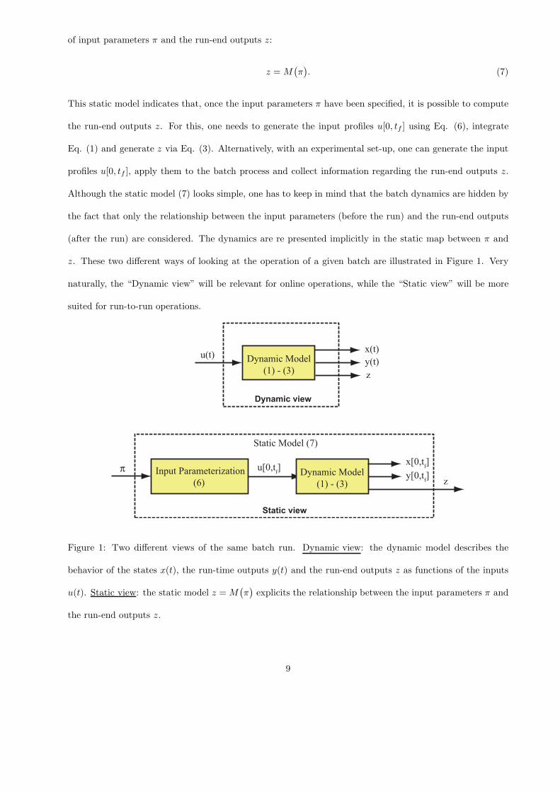
z. These two different ways of looking at the operation of a given batch are illustrated in Figure 1. Very

naturally, the “Dynamic view” will be relevant for online operations, while the “Static view” will be more

suited for run-to-run operations.

x(t)u(t)

y(t)

z

x[0,tf]

u[0,tf]

y[0,tf]

z

π

Static view

Dynamic Model

(1) - (3)

Dynamic Model

(1) - (3)

Dynamic view

Static Model (7)

Input Parameterization

(6)

Figure 1: Two different views of the same batch run. Dynamic view: the dynamic model describes the

behavior of the states x(t), the run-time outputs y(t) and the run-end outputs z as functions of the inputs

u(t). Static view: the static model z = M(

π)

explicits the relationship between the input parameters π and

the run-end outputs z.

9

PART A. CONTROL

Batch process control has gained popularity over the past forty years. This is due to the development of novel

algorithms with proven ability to improve the performance of industrial processes despite uncertainty and

perturbations. But the development of new sensors and of automation tools also contributed to this success.

At this stage, it is important to distinguish between control and automation. In practice, industry often

tends to consider that control and automation are two identical topics and use the two words interchangeably.

Although arguable, we will consider hereafter that control corresponds to the theory, that is, the research

field, whereby new control methods, algorithms and controller structures are sought. On the other hand,

automation represents the technology (the set of devices and their organization) that is needed to program

and implement control solutions.

The control of batch processes differs from the control of continuous processes because of the two

main distinguishing features presented in Section 2. First, since batch processes have no steady-state operat-

ing point, the setpoints to track are time-varying trajectories. Second, batch processes are repeated over time

and are characterized by two independent variables, the run time t and the run index k. The independent

variable k provides additional degrees of freedom for meeting the control objectives when these objectives do

not necessarily have to be completed in a single batch but can be distributed over several successive batches.

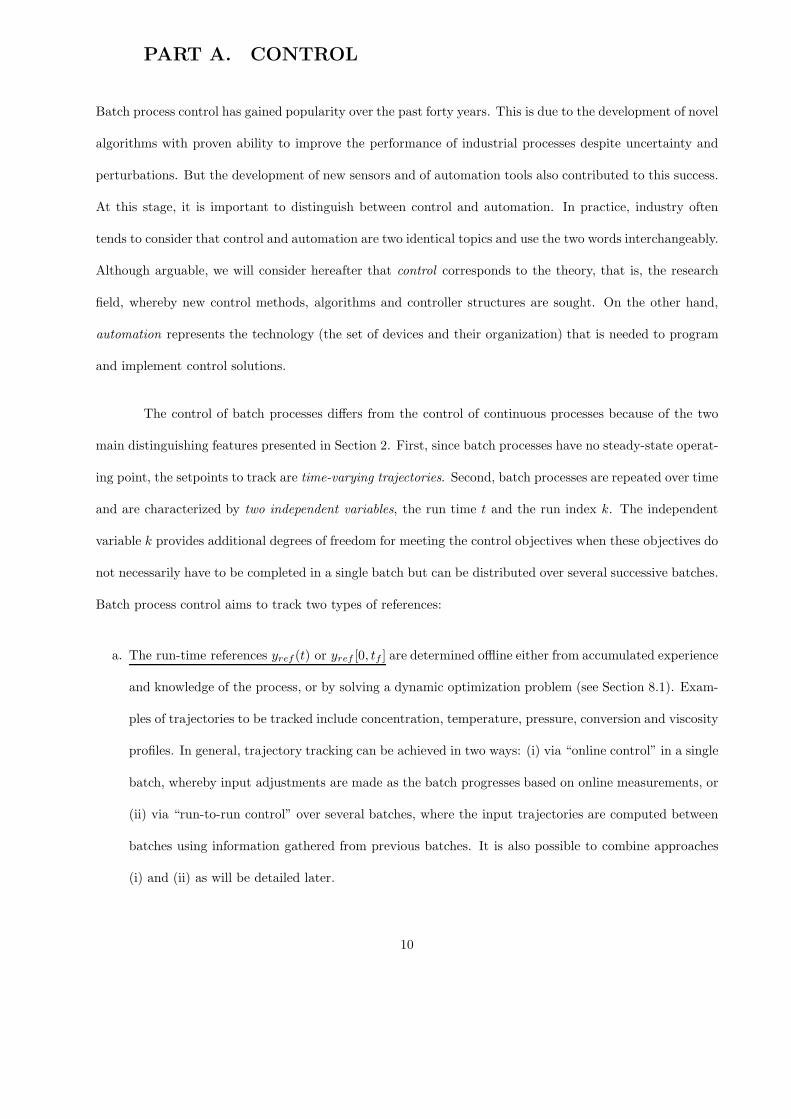
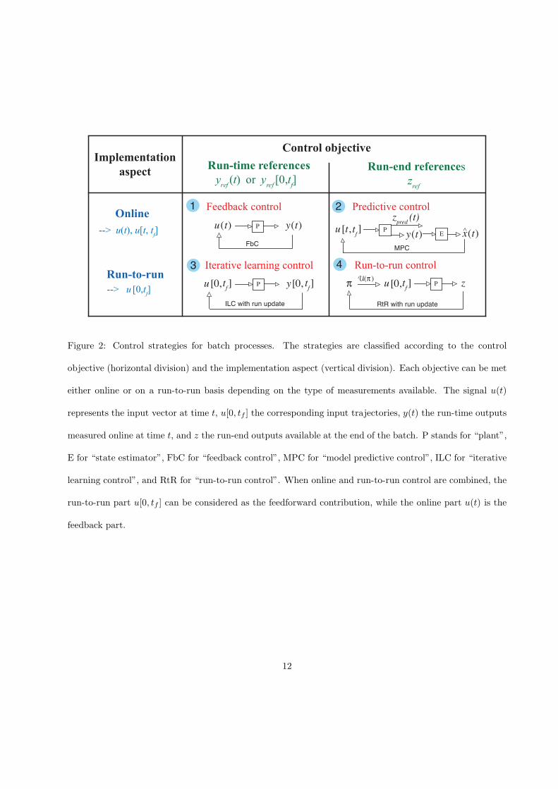
Batch process control aims to track two types of references:

a. The run-time references yref (t) or yref [0, tf ] are determined offline either from accumulated experience

and knowledge of the process, or by solving a dynamic optimization problem (see Section 8.1). Exam-

ples of trajectories to be tracked include concentration, temperature, pressure, conversion and viscosity

profiles. In general, trajectory tracking can be achieved in two ways: (i) via “online control” in a single

batch, whereby input adjustments are made as the batch progresses based on online measurements, or

(ii) via “run-to-run control” over several batches, where the input trajectories are computed between

batches using information gathered from previous batches. It is also possible to combine approaches

(i) and (ii) as will be detailed later.

10

b. The run-end references zref are associated with the run-end outputs that are only available at the end

of the batch. The most common run-end outputs are product quality, productivity and selectivity. As

with run-time references, the run-end references can be tracked online or on a run-to-run basis.

With these two types of control objectives and the two different ways of reaching them (online and over

several runs), there are four different control strategies as illustrated in Figure 2. It is interesting to see what

view (dynamic or static) each control strategy uses. It turns out that Strategies 1-3 use a dynamic view

of the batch process, with only Strategy 4 based on the static view. In the following, Section 4 addresses

online control (the first row in Figure 1, Strategies 1 and 2), while Section 5 deals with run-to-run control

(the second row in Figure 1, Strategies 3 and 4).

4 Online Control

The idea of “online control” is to take corrective action during the batch, that is, in run-time t. It is possible

to do so with two objectives in mind, namely, the run-time reference trajectories yref (t) and the run-end

references zref . This will be discussed in the next two subsections.

4.1 Feedback Control of Run-time Outputs (Strategy 1)

We will address successively the application of conventional feedback control to batch processes, the thermal

control of batch reactors, and the stability issue for batch processes.

4.1.1 Conventional feedback control

The application of online feedback control to batch processes has the peculiarity that the setpoints are often

time-varying trajectories. Even if some of the controlled variables, such as the temperature in isothermal

operation, remain constant, the key process parameters (static gains, time constants and time delays) can

11

Run-end references

zref

Run-time references

yref

(t) or yref

[0,tf]

Control objective

Feedback control 1

Iterative learning control

2

Run-to-run control4

Implementation

aspect

Online

--> u(t), u[t, tf]

Run-to-run

--> u [0,t

f]

Predictive control

3

u ( t ) y(t)

FbC

P

u [0, y[0, tf]t

f]

ILC with run update

P [0, ztf]u

RtR with run update

πU (π )

P

E x(t)^

MPC

u [t, tf] P

y(t)

zpred (t)

Figure 2: Control strategies for batch processes. The strategies are classified according to the control

objective (horizontal division) and the implementation aspect (vertical division). Each objective can be met

either online or on a run-to-run basis depending on the type of measurements available. The signal u(t)

represents the input vector at time t, u[0, tf ] the corresponding input trajectories, y(t) the run-time outputs

measured online at time t, and z the run-end outputs available at the end of the batch. P stands for “plant”,

E for “state estimator”, FbC for “feedback control”, MPC for “model predictive control”, ILC for “iterative

learning control”, and RtR for “run-to-run control”. When online and run-to-run control are combined, the

run-to-run part u[0, tf ] can be considered as the feedforward contribution, while the online part u(t) is the

feedback part.

12

vary considerably during the duration of the batch.

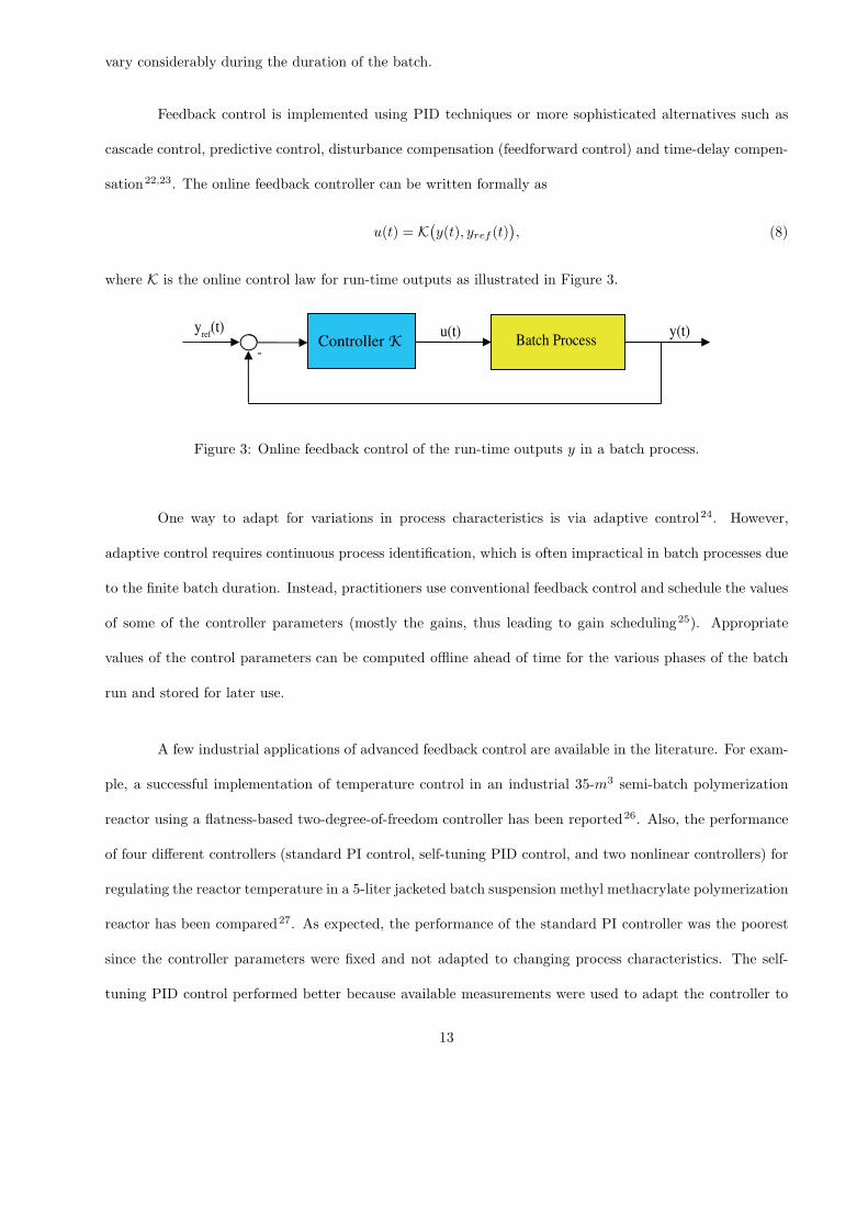
Feedback control is implemented using PID techniques or more sophisticated alternatives such as

cascade control, predictive control, disturbance compensation (feedforward control) and time-delay compen-

sation22,23. The online feedback controller can be written formally as

u(t) = K(

y(t), yref (t))

, (8)

where K is the online control law for run-time outputs as illustrated in Figure 3.

Controller K Batch Processy(t)u(t)y

ref(t)

Figure 3: Online feedback control of the run-time outputs y in a batch process.

One way to adapt for variations in process characteristics is via adaptive control24. However,

adaptive control requires continuous process identification, which is often impractical in batch processes due

to the finite batch duration. Instead, practitioners use conventional feedback control and schedule the values

of some of the controller parameters (mostly the gains, thus leading to gain scheduling25). Appropriate

values of the control parameters can be computed offline ahead of time for the various phases of the batch

run and stored for later use.

A few industrial applications of advanced feedback control are available in the literature. For exam-

ple, a successful implementation of temperature control in an industrial 35-m3 semi-batch polymerization

reactor using a flatness-based two-degree-of-freedom controller has been reported26. Also, the performance

of four different controllers (standard PI control, self-tuning PID control, and two nonlinear controllers) for

regulating the reactor temperature in a 5-liter jacketed batch suspension methyl methacrylate polymerization

reactor has been compared27. As expected, the performance of the standard PI controller was the poorest

since the controller parameters were fixed and not adapted to changing process characteristics. The self-

tuning PID control performed better because available measurements were used to adapt the controller to

13

the varying process characteristics. The two nonlinear controllers, which were based on differential-geometric

techniques requiring full-state measurement28, showed excellent performance despite significant uncertainty

in the heat-transfer coefficient.

4.1.2 Control of heat generation

The control of exothermic reactions in batch reactors is a challenging problem that is tackled using one of

various operation modes29:

1) Isothermal batch operation. Most reaction systems are investigated isothermally in the laboratory.

For safety and selectivity reasons, pilot-plant and industrial reactors are also run isothermally at the same

temperature specifications. However, the transfer function between the jacket inlet temperature and the

reactor temperature depends on the amount of heat evolved, and it can become unstable for certain combi-

nations of the reaction parameters29. Adaptation of the controller parameters is therefore necessary. Most

often, this is done by using pre-computed values, that is, via gain scheduling. An energy balance around the

reactor is sometimes used to estimate the heat generated by the chemical reactions, which represents the

major disturbance for the control system. This estimate can then be used very effectively in a feedforward

scheme. It is important to mention that isothermal batch operation often exhibits low productivity because

it is limited by the maximal heat-generation rate (corresponding to the maximal heat-removal capacity of

the reactor vessel), which typically occurs initially for only a short period of time.

2) Isothermal semi-batch operation. The productivity of isothermal batch reactors can be increased

through semi-batch operation. This way, the reactant concentrations can be increased once the initial

phase characterized by the heat-removal limitation is over. For strongly exothermic reactions, semi-batch

operation has the additional advantage of improving the effective heat-removal capacity through feeding of

cold reactants. This, in turn, increases the productivity of the reactor by allowing higher temperatures.

Hence, isothermal semi-batch operation is often the preferred way of running discontinuous reactors in

industry. The temperature is controlled by manipulating the feedrate of the limiting reactant. However, the

14

system exhibits non-minimum phase behavior, that is, a flowrate increase of the cold feed first reduces the

temperature before the temperature raises due to higher reaction rates, which significantly complicates the

control30. Furthermore, in most semi-batch operations, it is useful to finish off with a batch phase so as to

fully consume the limiting reactant. Without a kinetic model, it is not obvious when to switch from the

semi-batch to the batch mode. Finally, although isothermal, the operation of a semi-batch reactor should

be such that the heat-removal constraint is never violated. This has forced industrial practice to be rather

conservative, with a temperature setpoint often chosen from adiabatic considerations.

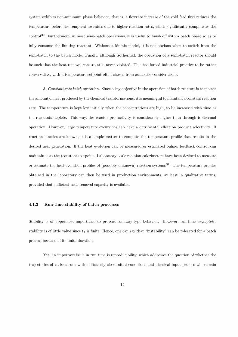
3) Constant-rate batch operation. Since a key objective in the operation of batch reactors is to master

the amount of heat produced by the chemical transformations, it is meaningful to maintain a constant reaction

rate. The temperature is kept low initially when the concentrations are high, to be increased with time as

the reactants deplete. This way, the reactor productivity is considerably higher than through isothermal

operation. However, large temperature excursions can have a detrimental effect on product selectivity. If

reaction kinetics are known, it is a simple matter to compute the temperature profile that results in the

desired heat generation. If the heat evolution can be measured or estimated online, feedback control can

maintain it at the (constant) setpoint. Laboratory-scale reaction calorimeters have been devised to measure

or estimate the heat-evolution profiles of (possibly unknown) reaction systems31. The temperature profiles

obtained in the laboratory can then be used in production environments, at least in qualitative terms,

provided that sufficient heat-removal capacity is available.

4.1.3 Run-time stability of batch processes

Stability is of uppermost importance to prevent runaway-type behavior. However, run-time asymptotic

stability is of little value since tf is finite. Hence, one can say that “instability” can be tolerated for a batch

process because of its finite duration.

Yet, an important issue in run time is reproducibility, which addresses the question of whether the

trajectories of various runs with sufficiently close initial conditions and identical input profiles will remain

15

close during the run. The problem of stability is in fact related to the sensitivity with respect to perturbations.

The basic framework for assessing this sensitivity is as follows:

• the system is perturbed by either variations of the initial conditions or external disturbances that affect

the system states,

• sensitivity is assessed as a norm indicating the relative effect of the perturbations.

For a system to be stable, this norm must remain bounded for a bounded perturbation, and it must go to

zero with time for a vanishing perturbation. However, when dealing with finite-time systems, it is difficult

to infer stability from this norm since, except for some special cases such as finite escape time, boundedness

is guaranteed. Also, the vanishing behavior with time cannot be analyzed since tf is finite. The element of

interest is in fact the numerical value of the norm, and the issue becomes quantitative rather than binary

(yes-no). Details can be found elsewhere15.

4.2 Predictive Control of Run-end Outputs (Strategy 2)

With a sufficiently accurate process model, and in the absence of disturbances, tracking the profiles de-

termined offline is often sufficient to meet the batch-end product quality requirements32. However, in the

presence of disturbances, following pre-specified profiles is unlikely to lead to the desired product quality.

Hence, the following question arises: Is it possible to design an online control scheme for effective control of

run-end outputs using run-time measurements? Since such an approach amounts to controlling a quantity

that has not yet been measured, it is necessary to predict run-end outputs to compute the required corrective

control action. Model predictive control (MPC) is well suited for the task of controlling future quantities that

need to be predicted33. This approach to batch control can, therefore, be formulated as an MPC problem

with a shrinking prediction horizon (equal to the remaining duration of the batch) and an objective function

that penalizes deviations from the desired product quality at batch end34.

16

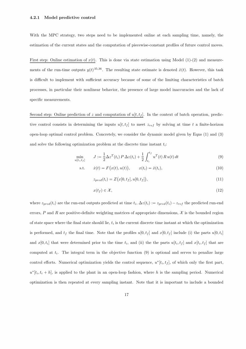
4.2.1 Model predictive control

With the MPC strategy, two steps need to be implemented online at each sampling time, namely, the

estimation of the current states and the computation of piecewise-constant profiles of future control moves.

First step: Online estimation of x(t). This is done via state estimation using Model (1)-(2) and measure-

ments of the run-time outputs y(t)35,36. The resulting state estimate is denoted x(t). However, this task

is difficult to implement with sufficient accuracy because of some of the limiting characteristics of batch

processes, in particular their nonlinear behavior, the presence of large model inaccuracies and the lack of

specific measurements.

Second step: Online prediction of z and computation of u[t, tf ]. In the context of batch operation, predic-

tive control consists in determining the inputs u[t, tf ] to meet zref by solving at time t a finite-horizon

open-loop optimal control problem. Concretely, we consider the dynamic model given by Eqns (1) and (3)

and solve the following optimization problem at the discrete time instant ti:

minu[ti,tf ]

J :=1

2∆zT (ti)P ∆z(ti) +

1

2

∫ tf

ti

uT (t)Ru(t) dt (9)

s.t. x(t) = F(

x(t), u(t))

, x(ti) = x(ti), (10)

zpred(ti) = Z(

x[0, tf ], u[0, tf ])

, (11)

x(tf ) ∈ X , (12)

where zpred(ti) are the run-end outputs predicted at time ti, ∆z(ti) := zpred(ti)− zref the predicted run-end

errors, P and R are positive-definite weighting matrices of appropriate dimensions, X is the bounded region

of state space where the final state should lie, ti is the current discrete time instant at which the optimization

is performed, and tf the final time. Note that the profiles u[0, tf ] and x[0, tf ] include (i) the parts u[0, ti]

and x[0, ti] that were determined prior to the time ti, and (ii) the the parts u[ti, tf ] and x[ti, tf ] that are

computed at ti. The integral term in the objective function (9) is optional and serves to penalize large

control efforts. Numerical optimization yields the control sequence, u∗[ti, tf ], of which only the first part,

u∗[ti, ti + h], is applied to the plant in an open-loop fashion, where h is the sampling period. Numerical

optimization is then repeated at every sampling instant. Note that it is important to include a bounded

17

region for the final states for the sake of stability33.

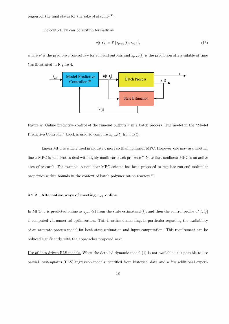
The control law can be written formally as

u[t, tf ] = P(

zpred(t), zref)

, (13)

where P is the predictive control law for run-end outputs and zpred(t) is the prediction of z available at time

t as illustrated in Figure 4.

Model Predictive

Controller P Batch Process y(t)

zref

State Estimation

x(t)

‹

zu[t, t

f]

Figure 4: Online predictive control of the run-end outputs z in a batch process. The model in the “Model

Predictive Controller” block is used to compute zpred(t) from x(t).

Linear MPC is widely used in industry, more so than nonlinear MPC. However, one may ask whether

linear MPC is sufficient to deal with highly nonlinear batch processes? Note that nonlinear MPC is an active

area of research. For example, a nonlinear MPC scheme has been proposed to regulate run-end molecular

properties within bounds in the context of batch polymerization reactors37.

4.2.2 Alternative ways of meeting zref online

In MPC, z is predicted online as zpred(t) from the state estimates x(t), and then the control profile u∗[t, tf ]

is computed via numerical optimization. This is rather demanding, in particular regarding the availability

of an accurate process model for both state estimation and input computation. This requirement can be

reduced significantly with the approaches proposed next.

Use of data-driven PLS models. When the detailed dynamic model (1) is not available, it is possible to use

partial least-squares (PLS) regression models identified from historical data and a few additional experi-

18

ments38. Then, in real time during the progress of the batch, it is possible to use the PLS model to estimate

the run-end outputs and track zref by adjusting u[t, tf ] via run-to-run control (see Section 5.2).

Another less ambitious but very efficient control approach has also been proposed, whereby, if the prediction

of z falls outside a predefined no-control region, a mid-course correction is implemented39. Note that the

approach can easily be modified to accommodate more than one mid-course correction.

Still another variant of the use of PLS models involves controlling the process in the reduced space (scores)

of a latent variable model rather than in the space of the discretized inputs40.

Use of online tracking. An alternative for meeting run-end references using online measurements consists

in tracking some feasible trajectory, zref (t), whose main purpose is to enforce zref at final time, that is,

zref (tf ) = zref41. This necessitates to be able to measure or estimate z(t) during the batch.

5 Run-to-run Control

Run-to-run control takes advantage of the repetition of batches that is characteristic of batch processing.

One uses information from previous batches to improve the performance of the next batch. This can be

achieved with respect to both run-time and run-end objectives, as discussed in the next two subsections.

5.1 Iterative Learning Control of Run-time Profiles (Strategy 3)

The time profiles of the manipulated variables can be generated using Iterative Learning Control (ILC),

which exploits information from previous runs to improve the performance of the current run42. This

strategy exhibits the limitations of open-loop control with respect to the current run, in particular the

fact that there is no feedback correction for run-time disturbances. Nevertheless, this scheme is useful for

generating time-varying feedforward input terms. The ILC controller has the formal structure

uk+1[0, tf ] = I(

yk[0, tf ], yref [0, tf ])

, (14)

19

where I is the ILC law for run-time outputs. ILC uses the entire profiles of the previous run to generate the

input profiles for the next run as illustrated in Figure 5. ILC has been successfully applied in robotics43,44

and in batch chemical processing45,46.

ILC

Controller I Batch Process

uk [0, t

f]

k+1 --> ku

k+1[0, t

f] y

k [0, t

f]y

ref [0, t

f]

Figure 5: ILC of the run-time profiles yk[0, tf ] in a batch process. The run update is indicated by k+1 → k.

5.1.1 ILC problem formulation

A repetitive batch process is considered in operator notation:

yk[0, tf ] = G(

uk[0, tf ], xk(0))

, (15)

where uk[0, tf ] and xk(0) represent the input profiles and the initial conditions in run k, G is the operator

representing the system. This relationship can be obtained from Model (1)-(2) as follows:

• With the inputs uk[0, tf ] and the initial conditions xk(0) specified, integrate Eq. (1) to obtain xk[0, tf ].

• Eq. (2) allows computing yk[0, tf ] from xk[0, tf ] and uk[0, tf ].

For the case where the system operator is linear and the signals are in discrete time, Eq. (15) can

be expressed in matrix form as follows:

yk = Guk + y0,k, (16)

with yk ∈ ℜNp, uk ∈ ℜNm and G ∈ ℜNp×Nm, where N is the finite number of time samples, p the number

of outputs, and m the number of inputs. y0,k ∈ ℜNp represents the response to the initial conditions xk(0).

ILC tries to improve trajectory following by utilizing the previous-cycle tracking errors. The ILC

update law for the inputs uk+1 is given as

uk+1 = Auk +Bek, ek = yref − yk, (17)

20

where yref ∈ ℜNp are the references to be tracked, and A ∈ ℜNm×Nm and B ∈ ℜNm×Np are operators

applied to the previous-cycle inputs and tracking errors, respectively. In the remainder of this section

dealing with ILC, the signals without an explicit time dependency are expressed as vectors containing the

N finite time samples, that is, uk ∈ ℜNm, yk ∈ ℜNp and ek ∈ ℜNp.

5.1.2 ILC convergence and residual errors

An ILC law is convergent if the following limits exist:

limk→∞

yk = y∞ and limk→∞

uk = u∞ . (18)

One way to ensure convergence is that the relation between uk and uk+1 be a contraction mapping in some

appropriate norm:

‖uk+1‖ ≤ ρ‖uk‖, 0 ≤ ρ < 1. (19)

Using (16) in Eq. (17) gives:

uk+1 = (A−BG) uk +B(yref − y0,k). (20)

Note that (yref − y0,k) does not represent errors as in Eq. (17), but the differences between the reference

trajectories and the responses to the initial conditions. Also, in contrast to Eq. (17), where ek depends on

uk through yk, (yref − y0,k) is independent of uk. Hence, the convergence of the algorithm depends on the

homogenous part of Eq. (20) and the condition for convergence is:

‖A−BG‖ < 1. (21)

If the iterative scheme converges, with uk = uk+1 = u∞ and y0,k = y0,k+1 = y0, Eq. (20) gives:

u∞ = (I −A+BG)−1 B(yref − y0). (22)

Since the converged outputs y∞ are not necessarily equal to the desired outputs yref , the final tracking

errors can be different from zero. The final tracking errors are given by

e∞ = yref − (Gu∞ + y0) =(

I −G (I −A+BG)−1

B)

(yref − y0). (23)

21

If BG is invertible, this equation can be rewritten as

e∞ = G(BG)−1(I −A) (I −A+BG)−1 B(yref − y0). (24)

Note that the residual errors are zero when A = I and non zero otherwise. Hence, the choice A = I provides

integral action along the run index k. Zero errors imply that perfect system inversion has been achieved.

5.1.3 ILC with current-cycle feedback

In conventional ILC schemes, only the tracking errors of the previous cycle are used to adjust the inputs in

the current cycle. To be able to reject within-run perturbations, the errors occurring during the current cycle

can be used as well, which leads to modified update laws. However, from the points of view of convergence

and error analysis, these modified schemes simply correspond to different choices of the operators A and B

in Eq. (17) as shown next. Let

uk+1 = uffk+1 + ufb

k+1, (25)

with uffk+1 = Auff

k + Bek, ufbk+1 = Cek+1, (26)

where the superscripts (·)ff and (·)fb are used to represent the feedforward and feedback parts of the inputs,

and A, B and C are operators.

Using Eq. (26) in Eq. (25) and combining it with Eqns (16)-(17) gives:

uk+1 = (I + CG)−1(

A(I + CG) − BG)

uk + (I + CG)−1(

B + C − AC)

(yref − y0)

=(

A−BG)

uk +B(yref − y0), (27)

where A = (I + CG)−1(A + CG) and B = (I + CG)−1(

B + (I − A)C)

. The convergence condition and

residual errors can be analyzed using the operators A and B, similarly to what was done in Section 5.1.2.

5.1.4 ILC with improved performance

The standard technique for approximate inversion is to introduce a forgetting factor in the input update47.

This causes the residual tracking errors to be non zero over the entire interval. Note, however, that the

22

main difficulty with the feasibility of inversion arises during the first part of the trajectory due to unmatched

initial conditions48. After a certain catch-up time, trajectory following is relatively easy. Hence, the idea is

to allow non-zero tracking errors early in the run and have the errors decrease progressively with run time t,

which can be achieved with an input shift. This is documented next as part of an ILC implementation that

includes (i) input shift, (ii) shift of the previous-cycle errors, and (iii) current-cycle feedback49.

The iterative update law is written as follows:

uk+1(t) = uffk+1(t) +Kfb ek+1(t), (28)

where Kfb ∈ ℜNm×Np are the proportional gains of the online feedback controller. The feedforward part of

the current inputs, uffk+1(t), consists of shifted versions of the feedforward part of the previous inputs and

the previous-cycle tracking errors:

uffk+1(t) = uff

k (t+ δu) +Kffek(t+ δe), (29)

where Kff ∈ ℜNm×Np are the proportional gains of the feedforward controller, δu the time shift of the

feedforward input trajectories and δe the time shift of the previous-run error trajectory. The remaining parts

of the inputs and errors are kept constant, that is, uffk [tf−δu, tf ] = uff

k (tf−δu) and ek[tf−δe, tf ] = ek(tf−δe),

respectively.

5.2 Run-to-run Control of Run-end Outputs (Strategy 4)

In this case, the interest is to steer the run-end outputs z towards zref using the input parameters π. For

this, one uses the static model (7) that results from the input parameterization (6). The run-to-run feedback

control law can be written as

πk+1 = R(

zk, zref)

, (30)

uk[0, tf ] = U(

πk, t)

, (31)

23

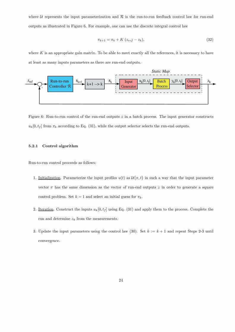
where U represents the input parameterization and R is the run-to-run feedback control law for run-end

outputs as illustrated in Figure 6. For example, one can use the discrete integral control law

πk+1 = πk +K (zref − zk), (32)

where K is an appropriate gain matrix. To be able to meet exactly all the references, it is necessary to have

at least as many inputs parameters as there are run-end outputs.

Run-to-run

Controller R

Batch

Process

zkuk[0, tf]Input

Generator

Output

Selector

yk[0, tf]πkk+1 --> k

Static Map

zref πk+1

Figure 6: Run-to-run control of the run-end outputs z in a batch process. The input generator constructs

uk[0, tf ] from πk according to Eq. (31), while the output selector selects the run-end outputs.

5.2.1 Control algorithm

Run-to-run control proceeds as follows:

1. Initialization. Parameterize the input profiles u(t) as U(

π, t)

in such a way that the input parameter

vector π has the same dimension as the vector of run-end outputs z in order to generate a square

control problem. Set k = 1 and select an initial guess for πk.

2. Iteration. Construct the inputs uk[0, tf ] using Eq. (31) and apply them to the process. Complete the

run and determine zk from the measurements.

3. Update the input parameters using the control law (30). Set k := k + 1 and repeat Steps 2-3 until

convergence.

24

5.2.2 Convergence analysis

The convergence of the run-to-run algorithm can be determined by analyzing the closed-loop error dynamics,

where the errors are ek := zref − zk.

We discuss next a convergence analysis that considers a linearized version of System (7) and the

linear integral control law (32). With the linear model,

zk = S πk, (33)

where S = ∂M∂π

∣

∣

πis the sensitivity matrix computed at the nominal operating point corresponding to π, the

linearized error dynamics become:

ek+1 = ek − SKek = (I − SK)ek. (34)

The eigenvalues of the matrix (I − S K) should be within the unit circle for the algorithm to converge.

Convergence is determined by both the sensitivity matrix S and the controller gainsK. Convergence analysis

of run-to-run control algorithms is also possible when the relationship between πk and zk is nonlinear, but

it typically requires additional assumptions regarding the nature of the nonlinearities50.

5.2.3 Run-to-run stability

The interest in studying stability in the run index k arises from the necessity to guarantee convergence of

run-to-run control schemes. Here, the standard notion of stability applies as the independent variable k goes

to infinity. The main conceptual difference with the stability of continuous processes is that “equilibrium”

refers to entire trajectories. Hence, the norms have to be defined in the space of functions L such as the

integral squared norm l2 of the signal x(t):

‖x[0, tf ]‖l2 =

∫ tf

0

(

x(t)2dt)1/2

. (35)

For studying stability with respect to the run index k, System (1) is considered under closed-loop

operation, that is, with all possible online and run-to run feedback loops. Hence, we no longer restrict our

25

attention to the input-output run-to-run π-z behavior, but we consider the entire state vector. For simplicity,

let us assume that tf is constant for all runs. When dealing with the kth run, the trajectories of the (k−1)st

run are known, which fixes uk[0, tf ] according to the ILC control law (14). These input profiles, along with

the online feedback law (8) or (13), are applied to System (1) to obtain xk(t) for all t and thus xk[0, tf ]. All

these operations can be represented formally as:

xk[0, tf ] = F(

xk−1[0, tf ])

, x0[0, tf ] = xinit[0, tf ], (36)

where xinit[0, tf ] are the initial state trajectories obtained by integration of Eq. (1) for k = 0, x0,0 = xinit

and u0[0, tf ] = uinit[0, tf ]. Eq. (36) describes the run-to-run dynamics associated with all control activities.

Run-to-run stability is considered around the equilibrium trajectory computed from (36), that is x[0, tf ] =

F(

x[0, tf ])

, and is investigated using a Lyapunov-function method51.

6 Batch Automation

Although batch processing was dominant until the 30’s, batch process control received significant interest

only 50 years later52. This is mainly due to the fact that, when control theory started to emerge in the 40’s,

there was a shift from the dominance of batch processing to continuous operations. Hence, the dynamics and

control of batch processes became a subject of investigation in the 80’s. Engineers then tried to carry over

to batch processes the experience gained over the years with the control of continuous processes. However,

the specificities of batch processes make their control quite challenging.

This is also true at the implementation level. If continuous processes typically exhibit four main

regimes, namely, start-up, continuous operation, possibly grade transition and shut down, batch processes

are much more versatile since, in the absence of a steady state, the system evolves freely from a set of initial

conditions to a final state. During this transient operation, the recipe can be rather varied, ranging from

basic isothermal operation to a succession of complex operations that can involve discrete decisions. Also,

batch processes are often repeated over time, with or without changes between batches, which makes the

task of designing a control strategy much more involved than for continuous operations.

26

The control of batch operations relies on various types of controllers that include stand-alone con-

trollers, programmable logic controllers (PLCs), distributed control systems (DCS), and personal computers

(PCs). These four platforms are discussed next.

6.1 Stand-alone Controllers

The basic stand-alone controllers are single-loop controllers (SLCs)53. These devices generally embed a

microprocessor with fixed functionalities such as PID control. The popularity of SLCs arose from their

simplicity, low cost and small size. Originally, stand-alone controllers were capable of integrating dual-

loop control, that is, they can handle two control loops with basic on/off and PID control. More recently,

these devices have incorporated self-tuning algorithms and, more importantly for batch processes, time

scheduling and sequencing functionalities. Still, the main advantage of SLCs is their low cost per control

loop. Furthermore, they are often used in parallel or in combination with more advanced control structures

such as DCS, mainly because they can achieve very acceptable control performance for minimal investment

regarding cost, maintenance and required knowledge.

6.2 Programmable Logic Controllers

PLCs were introduced in the process industries in the early 70’s, following the development in the automotive

industry, as computing systems “that had the flexibility of a computer, yet could be programmed and main-

tained by plant engineers and technicians”53. Before PLCs, relays, counters and timers were mainly used,

but they offered much less flexibility. PLCs can perform complex computations as they have a computational

power that is comparable to a small PC54.

Considerable progress was made with the introduction of micro-PLCs, which can be installed close to

the process at a much lower cost. The development of Supervisory Control and Data Acquisition (SCADA)

constitutes another breakthrough that has increased the scope of applications. It is possible to handle

numerous operations distributed over a large distance, thereby opening up the applicability of PLCs to cases

27

where batch process operations are fully integrated in the plant-wide operation of a production site.

6.3 Distributed Control Systems

DCS are control systems with control elements spread around the plant. They generally propose a hierarchical

approach to control, with several interconnected layers operating at different time scales. At the top of the

hierarchy is the production/scheduling layer, where the major decisions are taken on the basis of market

considerations and measurements collected from the plant. These decisions are sent to an intermediate layer,

where there are used, together with plant measurements and estimated fluctuations on price and raw-material

quality, to optimize the plant performance. These decisions can take the form of setpoint trajectories for

low-level controllers. This intermediate layer, which is often referred to as the real-time optimization layer, is

implemented via DCS55. Because of their distributed nature, DCS are helpful to integrate batch operations

into the continuous operation of a plant, which has considerable impact on the planning, scheduling and

real-time optimization tasks56. The control and optimization hardware has improved continuously over the

past decades, thereby keeping pace with the development of advanced control and optimization methods.

Although the differences between DCS and SCADA can appear to be subtle, one could state the

following56: DCS (i) are mainly process driven, (ii) are focused on small geographic areas, (iii) are suited

to large integrated chemical plants, (iv) rely on good data quality, and (v) incorporate powerful closed-loop

control hardware. On the other hand, SCADA is generally more “event driven”, which makes it more suited

to the supervision of multiple independent systems.

6.4 Personal Computers

PCs can also be used for the control and optimization of batch processes. It has been reported that 25% of

batch process control involve personal computers. Of course, this figure does not mean that 25% of batch

process control involves only PCs, as PCs are often used in combination with other controllers such as SLCs

or PLCs. In industry, PCs are not only used to program and run control algorithms, but they include

28

many other elements such as interfaces, communication protocols and networking53. The development of

user-friendly software interfaces, of simulation tools, and of fast and reliable optimization software has been

key to the development of batch processing. With the relatively low cost of PCs, it has become economically

viable to use them routinely for control. While a PC gives a lot of flexibility, especially for taking educated

decisions in the context of a multi-layered control structure, it can also be used as a stand-alone advanced

controller or even as an online optimization tool. In practice, however, PC-based control is often limited to

supervisory control, where the PC sends recommendations to low-level controllers. This can take the form of

input profiles to implement or of output trajectories to track during batch operation. These recommendations

can then be implemented directly by means of low-level controllers, or manually by an operator who can

take the final decision of implementing or not the recommendations53.

7 Control Applications

7.1 Control of Temperature and Final Concentrations in a Semi-batch Reactor

7.1.1 Reaction system

Consider the reaction of pyrrole A with diketene B to produce 2-acetoacetyl pyrrole C. Diketene is a very

aggressive compound that reacts with itself and other species to produce the undesired products D, E, and

F 57. The desired and side reactions are

A+ B → C,

2B → D,

C +B → E,

B → F.

The reactions are highly exothermic, that is, they produce heat. The reactor is operated in semi-batch mode

with A present initially in the reactor and B added with the feedrate profile u(t). Moreover, the reaction

29

system is kept isothermal by removing the heat produced by the chemical reactions through a cooling jacket

surrounding the reactor. The flowrate of cooling fluid is adjusted to keep the reactor temperature at its

desired setpoint.

7.1.2 Model of the reactor

The nonlinear dynamic model of the reaction system is obtained from a material balance for each species

and a total mass balance58:

dcAdt

= −u

VcA − k1cAcB, (37)

dcBdt

=u

V(cinB − cB)− k1cAcB − 2k2c

2B − k3cCcB − k4cB, (38)

dcCdt

= −u

VcC + k1cAcB − k3cCcB , (39)

dcDdt

= −u

VcD + k2c

2B, (40)

dcEdt

= −u

VcE + k3cCcB, (41)

dcFdt

= −u

VcF + k4cB, (42)

dV

dt= u, (43)

where ci is the concentration of the ith species, V is the reactor volume, kj is the rate constant of the jth

reaction, cinB is the inlet concentration of B, and u is the volumetric feedrate of B.

7.1.3 Control objective

One would like to operate the reactor safely and efficiently. If the heat produced cannot be removed by

the cooling jacket, the reactions accelerate and produce even more heat. This positive feedback effect,

known as thermal runaway, can result in high temperature and pressure and thus lead to an explosion;

this is precisely what caused the Bhopal disaster59. The performance of the reactor is evaluated by its

productivity, namely, the amount of desired product available at final time, as well as its selectivity, namely,

the portion of converted reactant B that forms the desired product C. Note that the performance criteria

30

(productivity and selectivity) are evaluated at the final time, whereas the manipulated variable (feedrate

of B) is a run-time profile. The control objective is to operate isothermally at 50 ◦C and match the final

concentrations cB,ref and cD,ref obtained in the laboratory

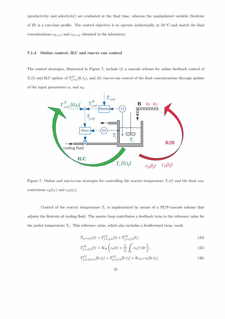
7.1.4 Online control, ILC and run-to run control

The control strategies, illustrated in Figure 7, include (i) a cascade scheme for online feedback control of

Tr(t) and ILC update of T ffj,ref [0, tf ], and (ii) run-to-run control of the final concentrations through update

of the input parameters u1 and u2.

cooling fluid

Slave

B Master

TT

TT

R2R

c B ( t f ) c D ( t f )

u1 u2

ILCTr

T ff

[0,tf] j,ref

[0,tf]

T fb j,ref

T r,ref

T j,ref

T r

T j

Figure 7: Online and run-to-run strategies for controlling the reactor temperature Tr(t) and the final con-

centrations cB(tf ) and cD(tf ).

Control of the reactor temperature Tr is implemented by means of a PI/P-cascade scheme that

adjusts the flowrate of cooling fluid. The master loop contributes a feedback term to the reference value for

the jacket temperature Tj . This reference value, which also includes a feedforward term, reads

Tj,ref,k(t) = T ffj,ref,k(t) + T fb

j,ref,k(t), (44)

T fbj,ref,k(t) = KR

(

ek(t) +1

τI

∫ t

0

ek(τ)dτ

)

, (45)

T ffj,ref,k+1[0, tf ] = T ff

j,ref,k[0, tf ] +KILC ek[0, tf ], (46)

31

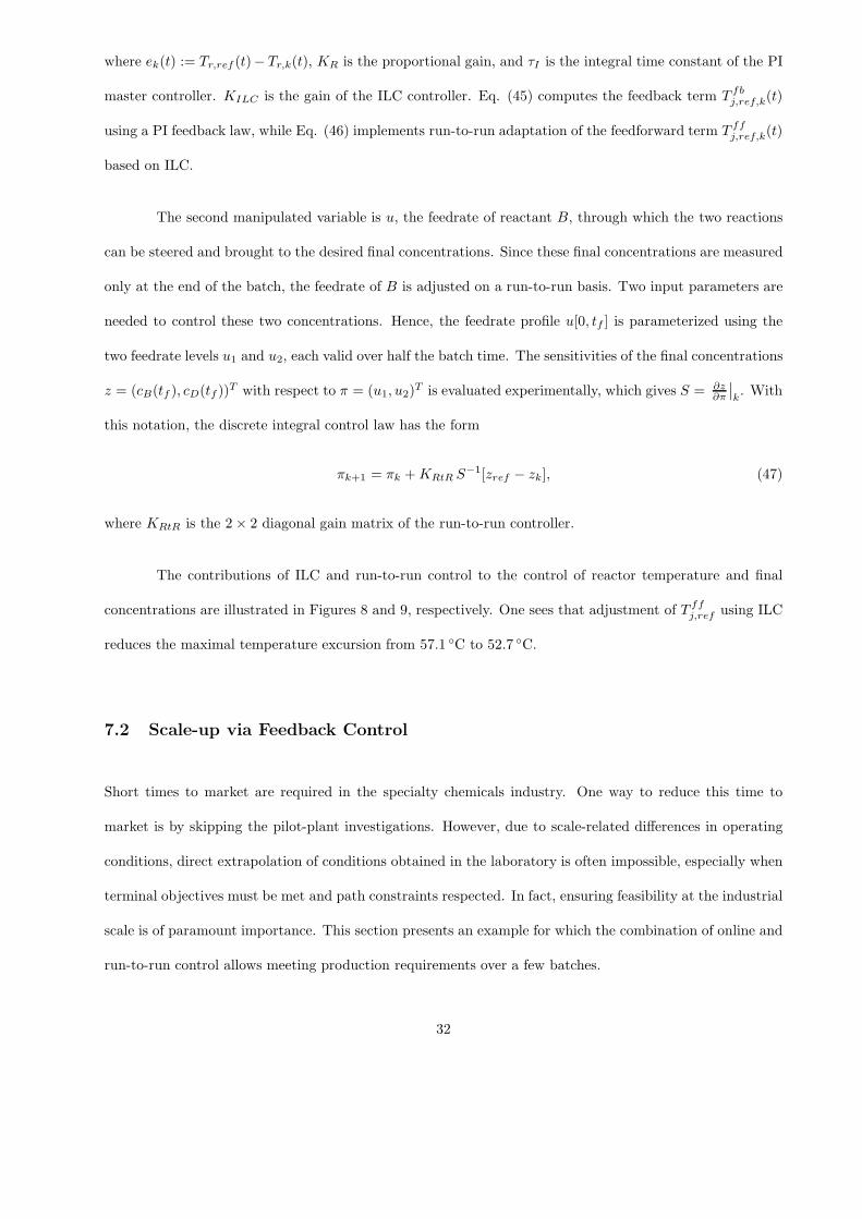
where ek(t) := Tr,ref (t)− Tr,k(t), KR is the proportional gain, and τI is the integral time constant of the PI

master controller. KILC is the gain of the ILC controller. Eq. (45) computes the feedback term T fbj,ref,k(t)

using a PI feedback law, while Eq. (46) implements run-to-run adaptation of the feedforward term T ffj,ref,k(t)

based on ILC.

The second manipulated variable is u, the feedrate of reactant B, through which the two reactions

can be steered and brought to the desired final concentrations. Since these final concentrations are measured

only at the end of the batch, the feedrate of B is adjusted on a run-to-run basis. Two input parameters are

needed to control these two concentrations. Hence, the feedrate profile u[0, tf ] is parameterized using the

two feedrate levels u1 and u2, each valid over half the batch time. The sensitivities of the final concentrations

z = (cB(tf ), cD(tf ))T with respect to π = (u1, u2)

T is evaluated experimentally, which gives S = ∂z∂π

∣

∣

k. With

this notation, the discrete integral control law has the form

πk+1 = πk +KRtR S−1[zref − zk], (47)

where KRtR is the 2× 2 diagonal gain matrix of the run-to-run controller.

The contributions of ILC and run-to-run control to the control of reactor temperature and final

concentrations are illustrated in Figures 8 and 9, respectively. One sees that adjustment of T ffj,ref using ILC

reduces the maximal temperature excursion from 57.1 ◦C to 52.7 ◦C.

7.2 Scale-up via Feedback Control

Short times to market are required in the specialty chemicals industry. One way to reduce this time to

market is by skipping the pilot-plant investigations. However, due to scale-related differences in operating

conditions, direct extrapolation of conditions obtained in the laboratory is often impossible, especially when

terminal objectives must be met and path constraints respected. In fact, ensuring feasibility at the industrial

scale is of paramount importance. This section presents an example for which the combination of online and

run-to-run control allows meeting production requirements over a few batches.

32

0 1 2 3 4

-10

10

30

50

70T [°C]

t [h]

tf0 1 2 3 4

-10

10

30

50

70T [°C]

t [h]

tf

Tj,refff

Tr

Tj,ref

Tj,ref

Tr

Tj,refff

Tj

Tj

Figure 8: Temperature control around the constant setpoint Tr,ref = 50 ◦C, without ILC (left), and after

three ILC iterations (right). The red and grey solid lines represents the reactor temperature Tr and the

jacket temperature Tj, respectively. The blue and green dashed lines represent the feedforward term of the

jacket temperature setpoint T ffj,ref and the resulting jacket temperature setpoint Tj,ref , respectively.

0 1 2 3 410

20

30

40

50

u [l/h]

t [h]

tf0 1 2 3 4

0

0.1

0..2

0..3

t [h]

tf

cB,ref

u1

u2

0 1 2 3 40

0.1

0..2

0..3

t [h]

tf

cD,ref

cDcB

Figure 9: Run-to-run control for meeting the run-end concentrations cB,ref and cD,ref . The inlet feedrate is

parameterized using the two levels u1 and u2 (left). The concentration profiles for cB(t) and cD(t) are shown

in the center and at right, respectively. The dashed lines show the initial profiles, while the solid lines show

the corresponding profiles after two iterations. The references cB,ref and cD,ref are reached via run-to-run

adjustment of u1 and u2.

33

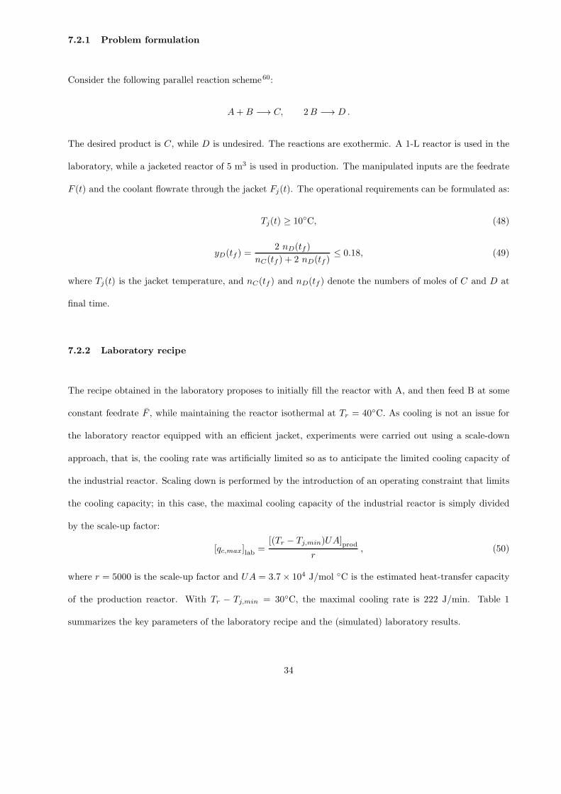
7.2.1 Problem formulation

Consider the following parallel reaction scheme60:

A+B −→ C, 2B −→ D .

The desired product is C, while D is undesired. The reactions are exothermic. A 1-L reactor is used in the

laboratory, while a jacketed reactor of 5 m3 is used in production. The manipulated inputs are the feedrate

F (t) and the coolant flowrate through the jacket Fj(t). The operational requirements can be formulated as:

Tj(t) ≥ 10◦C, (48)

yD(tf ) =2 nD(tf )

nC(tf ) + 2 nD(tf )≤ 0.18, (49)

where Tj(t) is the jacket temperature, and nC(tf ) and nD(tf ) denote the numbers of moles of C and D at

final time.

7.2.2 Laboratory recipe

The recipe obtained in the laboratory proposes to initially fill the reactor with A, and then feed B at some

constant feedrate F , while maintaining the reactor isothermal at Tr = 40◦C. As cooling is not an issue for

the laboratory reactor equipped with an efficient jacket, experiments were carried out using a scale-down

approach, that is, the cooling rate was artificially limited so as to anticipate the limited cooling capacity of

the industrial reactor. Scaling down is performed by the introduction of an operating constraint that limits

the cooling capacity; in this case, the maximal cooling capacity of the industrial reactor is simply divided

by the scale-up factor:

[qc,max]lab =[(Tr − Tj,min)UA]prod

r, (50)

where r = 5000 is the scale-up factor and UA = 3.7× 104 J/mol ◦C is the estimated heat-transfer capacity

of the production reactor. With Tr − Tj,min = 30◦C, the maximal cooling rate is 222 J/min. Table 1

summarizes the key parameters of the laboratory recipe and the (simulated) laboratory results.

34

Table 1: Laboratory recipe and results for the scale-up problem.

Recipe parameters Laboratory results

Tr = 40◦C cB,in = 5 mol/L nC(tf ) = 0.346 mol

cA,o = 0.5 mol/L cB,o = 0 mol/L yD(tf ) = 0.170

V0 = 1 L tf = 240 min maxt

qc(t) = 182.6 J/min

F = 4× 10−4 L/min

7.2.3 Scale-up via online control, ILC and run-to run control

The goal of scale-up is to reproduce in production the productivity and selectivity that are obtained in the

laboratory, while enforcing the desired reactor temperature. With selectivity and productivity as run-end

outputs, the feedrate profile F [0, tf ] is parameterized using two adjustable parameters, namely, the constant

feedrate levels F1 and F2, each one valid over half the batch time. Temperature control is done via a combined

feedforward/feedback scheme as illustrated in Section 7.1.

A control problem can be formulated with the following manipulated variables (MVs), controlled variables

(CVs) and setpoints (SPs):

• MVs: u(t) = Tj,ref (t), π =

[

F1, F2

]T

• CVs: y(t) = Tr(t), z =

[

nC(tf ), yD(tf )

]T

• SPs: yref = 40◦C, zref =

[

1630 mol, 0.17

]T

.

The setpoints are chosen as follows:

• Tr,ref = 40◦C is the value used in the laboratory.

• nC,ref is the value obtained in the laboratory multiplied by the scale-up factor r minus a 100-mol backoff

to account for scale-related uncertainties and run-time disturbances. The introduction of backoff makes

the control problem more flexible.

• yD,ref is the value obtained in the lab, which respects the upper bound of 0.18.

35

The control scheme is shown in Figure 10. The input profiles are updated using (i) the cascade feedback

controller K to control the reactor temperature Tr(t) online, (ii) the ILC controller I to improve the reactor

temperature by adjusting T ffj,ref (t) , and (iii) the run-to-run controllerR to control z = [ nC(tf ), yD(tf ) ]T

by adjusting π = [ F1, F2]T . Details regarding the implementation of the different control elements can

be found elsewhere60.

OnlineMeasurements

Online

R

Run-to-run

K

I

Run-endMeasurements

BatchProcess

TrajectoryGeneration

RunUpdate

Tj,ref,k+1

[0,tf]

ff

Tj,ref,k

(t)ff

Tj,ref,k

(t)fb

Tj,ref,k

(t)T

j,ref,k(t)

F1,k+1

, F2,k+1

F1,k

, F2,k

Fk(t)

Tr,ref

Tr,k

(t)

nC,ref

yD,ref

Tr,ref

xk(t)

xk[0,t

f]

ek(t)

ek[0,t

f]

+

+

nC,k

(tf)

yD,k

(tf)

Figure 10: Control scheme for scale-up implementation. Notice the distinction between online and run-to-

run activities. The symbol ∇ represents the concentration/expansion of information between a profile (e.g.

xk[0, tf ]) and an instantaneous value (e.g. xk(t)).

7.2.4 Simulation results

The recipe presented in Table 1 is applied to the 5-m3 industrial reactor, equipped with a 2.5-m3 jacket.

In this simulated case study, uncertainty is introduced artificially by modifying the two kinetic parame-

ters, which are reduced by 25% and 20%, respectively. Also, Gaussian noise with standard deviations of

0.001 mol/L and 0.1 ◦C is considered for the measurement of the final concentrations and for the reactor

temperature, respectively. It turns out that, for the first run, application of the laboratory recipe with

36

π =[

r F , r F]T

violates of the final selectivity of D in the first batch. Upon adapting the MVs with the

proposed scale-up algorithm, the free parts of the recipe are modified iteratively to achieve the production

targets for the industrial reactor, as illustrated in Figure 11.

yD

(tf)

5 10 150.165

0.17

0.175

0.18

0.185

Batch index

nC

(tf)

1520

1560

1600

1640

1480

Figure 11: Evolution of the production of C, nC(tf ), and the yield of D, yD(tf ), for the large-scale industrial

reactor. Most of the improvement is achieved in the first 7 runs (the dashed lines represent the target values).

7.3 Control of a Batch Distillation Column

A binary batch distillation column is used to illustrate in simulation the application of iterative learning

control. This example is described in detail elsewhere61.

7.3.1 Model of the column

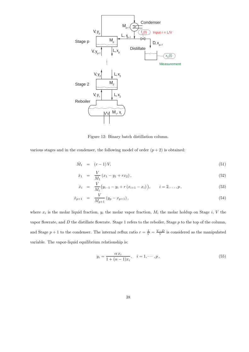
A binary batch distillation column with p equilibrium stages is considered (see Figure 12). Using standard

assumptions62 and writing molar balance equations for the holdup in the reboiler and for the liquid on the

37

Stage p

Reboiler

Stage 2

Condenser

Distillate

Measurement

Input r = L/V

M2

Mp

Mp+1

V, y1

V, yp-1

V, y2

V, yp

M1, x

1

L, xp

L, x3

L, x2

L, xp+1

D, xp+1

fD(t)

xD(t)

Figure 12: Binary batch distillation column.

various stages and in the condenser, the following model of order (p+ 2) is obtained:

M1 = (r − 1)V, (51)

x1 =V

M1(x1 − y1 + rx2) , (52)

xi =V

Mi

(

yi−1 − yi + r (xi+1 − xi))

, i = 2, . . . , p , (53)

xp+1 =V

Mp+1(yp − xp+1) , (54)

where xi is the molar liquid fraction, yi the molar vapor fraction, Mi the molar holdup on Stage i, V the

vapor flowrate, and D the distillate flowrate. Stage 1 refers to the reboiler, Stage p to the top of the column,

and Stage p+ 1 to the condenser. The internal reflux ratio r = LV = V−D

V is considered as the manipulated

variable. The vapor-liquid equilibrium relationship is:

yi =αxi

1 + (α− 1)xi, i = 1, · · · , p , (55)

38

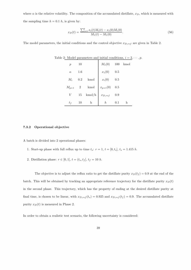
where α is the relative volatility. The composition of the accumulated distillate, xD, which is measured with

the sampling time h = 0.1 h, is given by:

xD(t) =

∑pi=1 xi(t)Mi(t)− xi(0)Mi(0)

M1(t)−M1(0). (56)

The model parameters, the initial conditions and the control objective xD,ref are given in Table 2.

Table 2: Model parameters and initial conditions, i = 2, · · · , p.

p 10 M1(0) 100 kmol

α 1.6 x1(0) 0.5

Mi 0.2 kmol xi(0) 0.5

Mp+1 2 kmol xp+1(0) 0.5

V 15 kmol/h xD,ref 0.9

tf 10 h h 0.1 h

7.3.2 Operational objective

A batch is divided into 2 operational phases:

1. Start-up phase with full reflux up to time ts: r = 1, t = [0, ts], ts = 1.415 h.

2. Distillation phase: r ∈ [0, 1], t = (ts, tf ], tf = 10 h.

The objective is to adjust the reflux ratio to get the distillate purity xD(tf ) = 0.9 at the end of the

batch. This will be obtained by tracking an appropriate reference trajectory for the distillate purity xD(t)

in the second phase. This trajectory, which has the property of ending at the desired distillate purity at

final time, is chosen to be linear, with xD,ref (ts) = 0.925 and xD,ref (tf ) = 0.9. The accumulated distillate

purity xD(t) is measured in Phase 2.

In order to obtain a realistic test scenario, the following uncertainty is considered:

39

- Perturbation: The vapor rate fluctuates every 0.5 h following an uniform distribution in the range

V = [13, 17] kmol/h.

- Measurement noise: 5% multiplicative Gaussian noise is added to the product composition xD(t).

The values of the squared tracking error∑tf

tse2(t) and the final tracking error e(tf ) upon convergence

are averaged over 20 realizations of the perturbation and measurement noise. Also, the variance ve(tf ) of

the final tracking error is calculated from 20 realizations.

7.3.3 Trajectory tracking via ILC

Trajectory tracking involving a single output, xD(t), and a single input, r(t), is implemented on a run-to-run

basis via ILC. The initial input trajectory used for ILC is linear with r(ts) = 0.898 and r(tf ) = 0.877. The

residual tracking error cannot be reduced to zero for all times because of the non-zero tracking error at

time ts arising from uncertainties in the start-up phase, that is, xD(ts) 6= xD,ref (ts). As a consequence, the

ILC schemes that try to enforce zero residual tracking error do not converge in this case. Instead, non-zero

tracking error has to be tolerated to enforce convergence. This can be accomplished by applying a forgetting

factor or a time shift to the feedforward trajectory. Three ILC schemes without current-cycle feedback are

considered, with N = 100 time samples:

• β = 0.999. A forgetting factor β is applied to the feedforward input trajectory in Eq. (26) with A = β I

and B = K.

• δu = 0.25 h. A small shift is applied to the feedforward input trajectory in Eq. (29).

• δu = 1 h, δe = 1 h. The same large shift is applied to the feedforward input and the error trajectory in

Eq. (29).

The proportional gain K = 0.1 I is determined as a compromise between robustness and perfor-

mance. ILC with forgetting factor converges after 30 runs, while the schemes with time shift of the trajec-

tories converge after 25 runs as illustrated in Figure 13. The final tracking error is slightly smaller with the

40

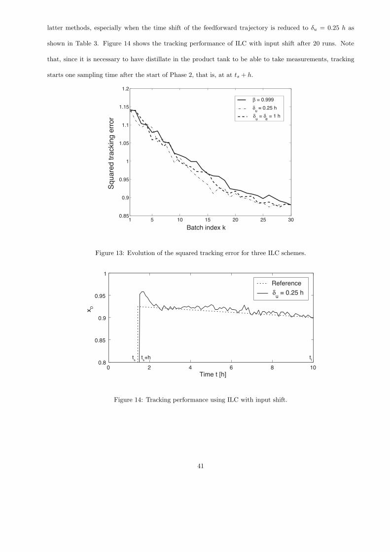
latter methods, especially when the time shift of the feedforward trajectory is reduced to δu = 0.25 h as

shown in Table 3. Figure 14 shows the tracking performance of ILC with input shift after 20 runs. Note

that, since it is necessary to have distillate in the product tank to be able to take measurements, tracking

starts one sampling time after the start of Phase 2, that is, at at ts + h.

1 5 10 15 20 25 300.85

0.9

0.95

1

1.05

1.1

1.15

1.2

Batch index k

β = 0.999

δu = 0.25 h

δu = δ

e = 1 h

Sq

ua

red

tra

ckin

g e

rro

r

Figure 13: Evolution of the squared tracking error for three ILC schemes.

0 2 4 6 8 100.8

0.85

0.9

0.95

1

Time t [h]

xD

Reference

δu = 0.25 h

ts

ts+h t

f

Figure 14: Tracking performance using ILC with input shift.

41

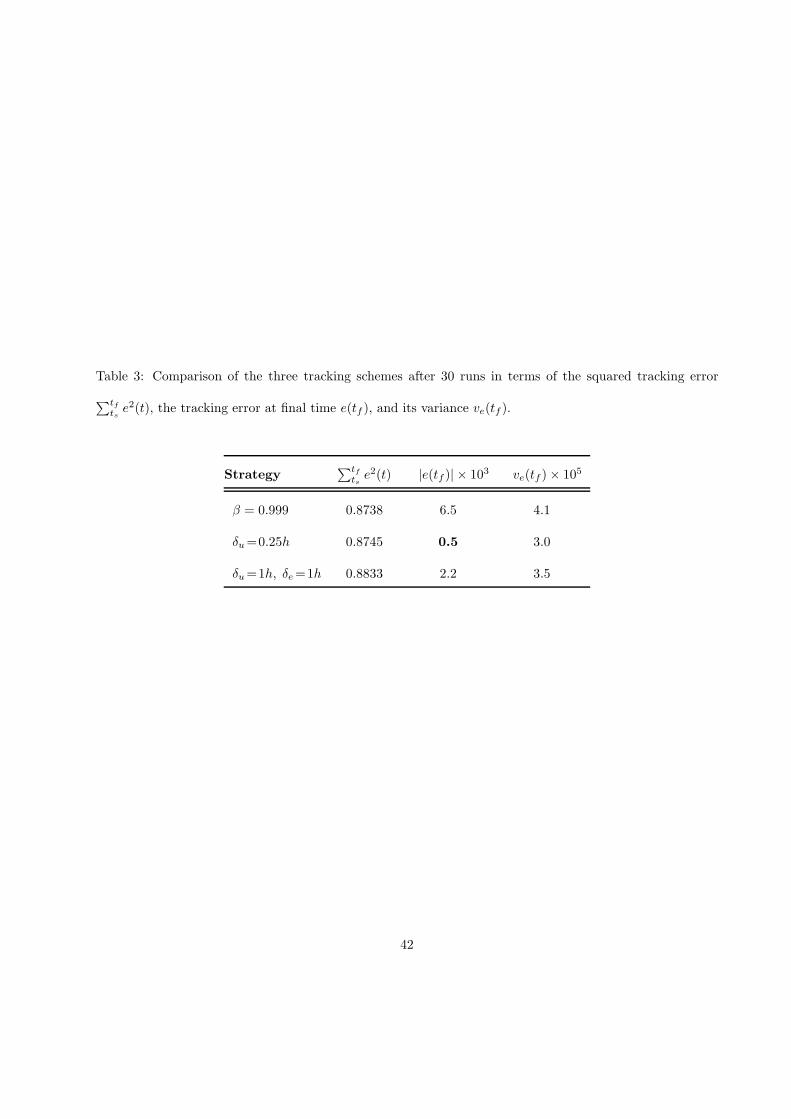
Table 3: Comparison of the three tracking schemes after 30 runs in terms of the squared tracking error

∑tftse2(t), the tracking error at final time e(tf ), and its variance ve(tf ).

Strategy∑tf

tse2(t) |e(tf )| × 103 ve(tf )× 105

β = 0.999 0.8738 6.5 4.1

δu=0.25h 0.8745 0.5 3.0

δu=1h, δe=1h 0.8833 2.2 3.5

42

PART B. OPTIMIZATION

Process optimization is the method of choice for improving the performance of chemical processes while

enforcing operational constraints63. Long considered as an appealing tool but only applicable to academic

problems, optimization has now become a viable technology64,65. Still, one of the strengths of optimization,

namely, its inherent mathematical rigor, can also be perceived as a weakness, since engineers might some-

times find it difficult to obtain an appropriate mathematical formulation to solve their practical problems.

Furthermore, even when process models are available, the presence of plant-model mismatch and process

disturbances makes the direct use of model-based optimal inputs hazardous.

In the last 30 years, the field of real-time optimization (RTO) has emerged to help overcome the

aforementioned modeling difficulties. RTO integrates process measurements into the optimization framework.

This way, process optimization does not rely exclusively on a (possibly inaccurate) process model but also on

process information stemming from measurements. The first widely available RTO approach was the two-

step approach that adapts the model parameters on the basis of differences between predicted and measured

outputs and uses the updated process model to re-compute the optimal inputs66,67. However, in the presence

of structural plant-model mismatch, this method is very unlikely to drive the plant to optimality68,69. Hence,

alternatives to the two-step approach have recently been developed. For example, the modifier-adaptation

scheme also proposes to solve a model-based optimization problem, but using a plant model with fixed

model parameters69. Correction for uncertainty is made via modifier terms that are added to the cost and

constraint functions of the optimization problem. As the modifiers include information on the differences

between the predicted and the plant necessary conditions of optimality (NCO), this approach is prone to

reach the plant optimum upon convergence. Yet another field has emerged, for which numerical optimization

is not used online. With the so-called self-optimizing approaches70–72, the optimization problem is recast

as a control problem that uses measurements to enforce certain optimality features for the plant. However,

note that self-optimizing control70 and extremum-seeking control71, which have been developed to optimize

continuous plants, are not suited to the optimization of batch processes.

43

The optimization of a batch process falls naturally in the category of dynamic optimization, that is,

with infinite-dimensional time profiles as decision variables. However, the introduction of input parameteri-

zation can transform the dynamic optimization problem into a static optimization problem with a countable

number of decision variables, a so-called nonlinear program (NLP).

This optimization part is organized as follows. Various aspects of numerical optimization for both

static and dynamic optimizations are presented first, followed by a discussion of two RTO classes, namely, re-

peated numerical optimization and optimizing control. The theoretical developments will then be illustrated

by three case studies.

8 Numerical Optimization

Apart from very specific cases, the standard way of solving an optimization problem is via numerical opti-

mization, for which a model of the process is required. As already mentioned, the optimization of a batch

process can be formulated as a dynamic optimization problem. In this chapter, we will consider the following

constrained dynamic optimization problem:

minu[0,tf ]

J := φ(

x(tf ))

(57)

s.t. x(t) = F(

x(t), u(t))

, x(0) = x0, (58)

S(

x(t), u(t))

≤ 0, (59)

T(

x(tf ))

≤ 0, (60)

where φ is the terminal-time cost functional to be minimized, x(t) the n-dimensional vector of state profiles

with the known initial conditions x0, u(t) the m-dimensional vector of input profiles, S the nS-dimensional

vector of path constraints that hold during the interval [0, tf ], T the nT -dimensional vector of terminal

constraints that hold at tf , and tf the final time, which can be either free or fixed†. The optimization

†If tf is free, it becomes a decision variable. Note that it is also possible to have additional constant decision variables. In this

case, the decision variables would include the vector of input profiles u[0, tf ] and the vector of constant quantities, ρ. This

general case will not be considered here for simplicity of exposition, see72 for details.

44

problem (57)-(60) is said to be in the Mayer form, that is, J is a terminal-time cost. When an integral cost

is added to φ , the corresponding problem is said to be in the Bolza form, while when it only incorporates

the integral cost, it is referred to as being in the Lagrange form. Note that these three formulations can be

made equivalent by the introduction of additional states73.

The nonlinear dynamic optimization problem (57)-(60) is difficult to solve due to the time depen-

dency of the various variables. In particular, the inputs u(t) represent an infinite-dimensional decision

vector. This time dependency can be removed via time discretization using, for example, the method of

orthogonal collocation74, which however results in a large vector of decision variables. Another approach

consists in viewing the batch process as a static map between a small number of input parameters π and a

small number of run-end outputs z as discussed in Section 3.3. These approximations reduce the dynamic

optimization problem into a static problem. Next, the following problems will be addressed successively:

dynamic optimization, reformulation of a dynamic optimization problem as a static optimization problem,

static optimization, and effect of uncertainty.

8.1 Dynamic Optimization

Consider the optimization problem (57)-(60), for which we will present the necessary conditions of optimality.

8.1.1 Pontryagin’s minimum principle

The NCO for a dynamic optimization problem are given by Pontryagin’s minimum principle (PMP). The

application of PMP provides insight in the optimal solution and generates explicit conditions for meeting

active path and terminal constraints and forcing certain sensitivities to zero.

Let us define the Hamiltonian function H(t),

H(t) = λT (t)F(

x(t), u(t))

+ µT (t)S(

x(t), u(t))

, (61)

45

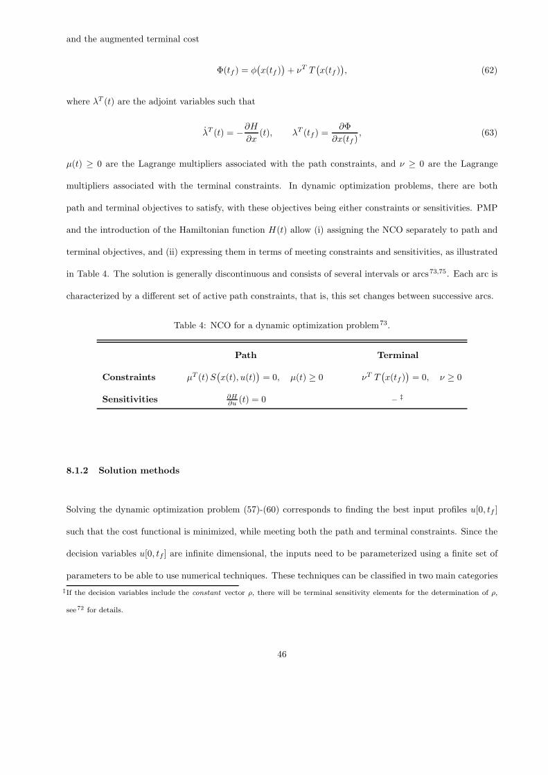
and the augmented terminal cost

Φ(tf ) = φ(

x(tf ))

+ νT T(

x(tf ))

, (62)

where λT (t) are the adjoint variables such that

λT (t) = −∂H

∂x(t), λT (tf ) =

∂Φ

∂x(tf ), (63)

µ(t) ≥ 0 are the Lagrange multipliers associated with the path constraints, and ν ≥ 0 are the Lagrange

multipliers associated with the terminal constraints. In dynamic optimization problems, there are both

path and terminal objectives to satisfy, with these objectives being either constraints or sensitivities. PMP

and the introduction of the Hamiltonian function H(t) allow (i) assigning the NCO separately to path and

terminal objectives, and (ii) expressing them in terms of meeting constraints and sensitivities, as illustrated

in Table 4. The solution is generally discontinuous and consists of several intervals or arcs73,75. Each arc is

characterized by a different set of active path constraints, that is, this set changes between successive arcs.

Table 4: NCO for a dynamic optimization problem73.

Path Terminal

Constraints µT (t)S(

x(t), u(t))

= 0, µ(t) ≥ 0 νT T(

x(tf ))

= 0, ν ≥ 0

Sensitivities ∂H∂u (t) = 0 – ‡

8.1.2 Solution methods

Solving the dynamic optimization problem (57)-(60) corresponds to finding the best input profiles u[0, tf ]

such that the cost functional is minimized, while meeting both the path and terminal constraints. Since the

decision variables u[0, tf ] are infinite dimensional, the inputs need to be parameterized using a finite set of

parameters to be able to use numerical techniques. These techniques can be classified in two main categories

‡If the decision variables include the constant vector ρ, there will be terminal sensitivity elements for the determination of ρ,

see72 for details.

46

according to the underlying formulation73, namely, direct optimization methods that solve the optimization

problem (57)-(60) directly, and PMP-based methods that attempt to satisfy the NCO given in Table 4.

Direct optimization methods are distinguished further depending on whether the system equations

are integrated explicitly or not73. In the sequential approach, the system equations are integrated explicitly,

and the optimization is carried out in the space of the decision variables only. This corresponds to a

“feasible-path” approach since the differential equations are satisfied at each step of the optimization. A

piecewise-constant or piecewise-polynomial approximation of the inputs is often used. The computationally

expensive part of the sequential approach is the accurate integration of the system equations, which needs

to be performed even when the decision variables are far from the optimal solution!

In the simultaneous approach, an approximation of the system equations is introduced to avoid explicit

integration for each candidate set of input profiles, thereby reducing the computational burden. Since

the optimization is carried out in the full space of discretized inputs and states, the differential equations

are satisfied only at the solution74,76. This is therefore called an “infeasible-path” approach. The direct

approaches are by far the most commonly used. However, note that the input parameterization is often

chosen arbitrarily by the user, which can affect both the efficiency and the accuracy of the approach77.

On the other hand, PMP-based methods try to satisfy the first-order NCO given in Table 4. The

NCO involve the state and adjoint variables, which need to be computed via integration. The differential

equation system is a two-point boundary-value problem since initial conditions are available for the states

and terminal conditions for the adjoints. The optimal inputs can be expressed analytically from the NCO

in terms of the states and the adjoints, that is, u∗[0, tf ] = U(

x[0, tf ], λ[0, tf ])

. The resulting differential-

algebraic system of equations can be solved using a shooting approach78, that is, the decision variables

include the initial conditions λ(0) that are chosen in order to satisfy λ(tf ).

47

8.2 Reformulation of a dynamic optimization problem as a static optimization

problem

Consider the optimization problem (57)-(60). Numerically, this problem can be solved by control vector

parameterization (CVP)76, whereby the infinite-dimensional inputs u(t) are parameterized using a finite

number of parameters π. Typically, the inputs are divided into small intervals, and a polynomial approxima-

tion of the inputs is used within each interval. The input parameter vector π can also include the switching

times between the intervals. It follows that the inputs can be expressed as u(t) = U(π, t) and the optimization

performed with respect to π, where π is the nπ-dimensional vector of constant decision variables.

The difficulty with such a parameterization is that the path constraints S(x, u) have to be discretized

as well, resulting in as many constraints as there are discretization points (typically a large number). However,

if structural information regarding the shape of the optimal solution is available, the path constraints can

be handled differently using an alternative parameterization as explained next.

The solution to a constrained terminal-time dynamic optimization problem is typically discontinuous

and consists of various arcs. For a given input, the ith arc ηi(t) can be of two types:

1. ηi,path : Arc ηi(t) is determined by an active path constraint (constraint-seeking arc),

2. ηi,sens : Arc ηi(t) is not governed by an active path constraint, it is sensitivity seeking.

Let us assume that the path constraints are met using either (i) assignment of input values in

the case of active input bounds, or (ii) online feedback control via the measurement or estimation of the

constrained quantities and their regulation to track the constraint values. The other parts of the inputs are

parameterized as in CVP as u(t) = U(π, t). Since the path constraints are handled directly, they do not

involve the decision variables π. Note that the knowledge of the active path constraints in various intervals

is crucial for this parameterization. The final states, which affect the objective function and the terminal

constraints, can be expressed in terms of the decision variables π as follows:

x(tf ) = x0 +

∫ tf

0

F(

x(t),U(π, t))

dt := F(π), (64)

48

as tf is an element of π. Hence, the dynamic optimization problem (57)-(60) can be reformulated as:

minπ

φ(

F(π))

(65)

s.t. T(

F(π))

≤ 0, (66)

since the system dynamics are included in F and the path constraints are taken care of as mentioned above.

It follows that the dynamic optimization problem can be reformulated as the following static NLP:

minπ

J := Φ(π) (67)

s.t. G(π) ≤ 0. (68)

The scalar cost function to be minimized is written Φ(π) := φ(

F(π))

, and the ng-dimensional vector of

constraints is written generically G(π) := T(

F(π))

.

Some remarks are necessary at this point:

• This reformulation is a mathematical way of viewing the dynamic process as a static input-output

“π-(Φ, G)” map. However, the process remains dynamic, with the terminal cost and the terminal

constraints being affected by the process dynamics.

• This reformulation is clearly an approximation since it relies on: (i) a parameterization of the inputs,

and (ii) approximate tracking of the state constraints.

• NLP (67)-(68) is a complex problem if one wants to predict Φ and G from π since the system dynamics

need to be integrated according to Eq. (64). However, the situation is much simpler in the experimental

context, as one simply apply the inputs π to the plant and measure both Φ and G. In this case, the

model used to predict Φ and G is replaced by the plant itself. This is a perfect example of the power

of measurement-based optimization compared to numerical optimization, as will be detailed later.

8.3 Static Optimization

The optimization problem is of algebraic nature with a finite number of constant decision variables.

49

8.3.1 KKT necessary conditions of optimality

With the formulation (67)-(68) and the assumption that the cost function Φ and the constraint functions G

are differentiable, the Karush-Kuhn-Tucker (KKT) conditions read79:

G(π∗) ≤ 0, (69)

∇Φ(π∗) + (ν∗)T∇G(π∗) = 0, (70)

ν∗ ≥ 0, (71)

(ν∗)TG(π∗) = 0, (72)

where π∗ denotes the solution, ν∗ the ng-dimensional vector of Lagrange multipliers associated with the

constraints, ∇Φ(π∗) the nπ-dimensional row vector denoting the cost gradient evaluated at π∗, and ∇G(π∗)

the (ng ×nπ)-dimensional Jacobian matrix computed at π∗. For these equations to be necessary conditions,

π∗ needs to be a regular point for the constraints, which calls for linear independence of the active constraints,

that is, rank{∇Ga(π∗)} = ng,a, where Ga represents the set of active constraints, whose cardinality is ng,a.

Condition (69) is the primal feasibility condition, Condition (71) the dual feasibility condition, and

Condition (72) the complementarity slackness condition. The stationarity condition (70) indicates that, at

the solution, collinearity between the cost gradient and a linear combination of the gradients of the active

constraints prevents from finding a search direction that would result in cost reduction while still keeping

the constraints satisfied.

8.3.2 Solution methods

Static optimization can be solved by state-of-the-art nonlinear programming techniques. In the presence

of constraints, the three most popular approaches are80: (i) penalty-function methods, (ii) interior-point

methods, and (iii) sequential quadratic programming. The main idea in penalty-function methods is to

replace the solution to a constrained optimization problem by the solution to a sequence of unconstrained

optimization problems. This is made possible by incorporating the constraints in the objective function via

50

a penalty term, which penalizes any violation of the constraints, while guaranteeing that the two problems

share the same solution (by selecting sufficiently large weights). Interior-point methods also incorporate the

constraints in the objective function81. However, the constraints are approached from the feasible region,

and the additive terms increase to become infinitely large at the value of the constraints, thereby acting more

like a barrier than a penalty term. A clear advantage of interior-point methods is that feasible iterates are

generated, while for penalty function methods, feasibility is only guaranteed upon convergence. Note that a

barrier-penalty function that combines the advantages of both approaches has also been proposed82. Another

way of computing the solution to a static optimization problem is to solve the set of NCO, for example

iteratively using sequential quadratic programming (SQP). SQP methods solve a sequence of optimization

sub-problems, each one minimizing a quadratic approximation to the Lagrangian function L := Φ + νTG

subject to a linear approximation of the constraints. SQP typically uses Newton’s or quasi-Newton methods

to solve the KKT conditions.

8.4 Effect of Uncertainty

8.4.1 Plant-model mismatch

The model used for optimization consists of a set of equations that represent an abstract view, yet always

a simplification, of the real process. Such a model is built based on conservations laws (for mass, numbers

of moles, energy) and constitutive relationships that express kinetics, equilibria and transport phenomena.

The simplifications that are introduced at the modeling stage to obtain a tractable model affect the quality

of the process model in two ways:

(i) some physical or chemical phenomena are assumed to be negligible and are discarded, and

(ii) some dynamic equations are assumed to be at quasi-steady state.

Hence, the structure of the model that is used differs from the “true” model structure. This di-

chotomy gives rise to the so-called structural plant-model mismatch. Furthermore, the model involves a

51

number of physical parameters, whose values are not known accurately. These parameters are identified

using process measurements and, consequently, are only known to belong to some interval with a certain

probability. For the sake of simplicity, we will consider thereafter that all modeling uncertainties, although

unknown, can be incorporated in the vector of uncertain parameters θ.

8.4.2 Model adequacy

Uncertainty is detrimental to the quality of both model predictions and optimal solutions. If the model

is not able to predict the process outputs accurately, it will most likely not be able to predict the NCO

correctly. On the other hand, even if the model is able to predict the process outputs accurately, it is often

unable to predict the NCO correctly since it has been trained to predict the outputs and not, for instance,

the gradients that are key constituents of the NCO. Hence, numerical optimization is capable of computing

optimal inputs for the model, but it often fails to reach plant optimality.

The property that ensures that a model-based optimization problem will be able to determine the

optimal inputs for the plant is referred to in the literature as “model adequacy”. For a given model-based

RTO scheme, a model is adequate if the RTO scheme is able to predict the correct set of active plant

constraints and the correct alignment of plant gradients. Model adequacy represents a major challenge

in process optimization since, as discussed earlier, models are trained to predict the plant outputs rather

than the plant NCO. In practice, application of model-based optimal inputs leads to suboptimal, and often

infeasible, operation.

9 Real-time Optimization

In the presence of modeling errors and process disturbances, the control trajectories computed offline lose

their optimal character. One way to reject the effect of uncertainty on the overall performance (with respect

to both optimality and feasibility) is by adequately incorporating process measurements in the optimization

52

framework. This is the field of real-time optimization. Measurements can be incorporated in two different

ways as illustrated in Figure 15:

a. Adapt the process model and repeat the optimization. At each iteration, the model parameters are

updated and the optimization problem solved numerically to generate u∗[0, tf ]. This adaptation and

optimization can also be repeated online, in a single run, to estimate at time t the current states x(t)

and compute the inputs u∗[t, tf ] for the remaining part of the batch.

b. Adapt the inputs through optimizing feedback control. Here, the optimization is implicit since opti-

mality and feasibility are enforced via feedback control to satisfy the necessary conditions of optimality.

The control scheme often involves (i) online elements that generate parts of the inputs, u∗a(t), and (ii)

run-to-run elements that generate the other part of the inputs, u∗b [0, tf ], via the input parameters π∗.

These RTO schemes will be discussed in the following subsections.

9.1 Repeated Numerical Optimization

As additional information about the process becomes available, either during or at the end of the run,

this information can be used to improve future operations. This will be documented next for both online

implementation using economic MPC and run-to-run implementation via the two-step approach.

9.1.1 Economic MPC (Strategy 1)

The approach is similar to MPC discussed in Section 4.2.1, but for the fact that the cost function is no longer

tailored to tracking run-end references, but rather to minimize an economic cost function. The problem can

53

Economic MPC1

2

3a Online NCO tracking

3bTwo-step approach

Optimizing feedback control

(track optimality conditions)

Repeated num. optim.

(of an updated model)

Run-to-run

Online

Implementation

aspect

Optimization via

Run-to-run NCO tracking

u [0,t

f] ∗

u (t), u

[t, t

f]∗

∗

u [0, y[0, tf]t

f]

Id. & Opt. for next run

P∗

ua ( t ) y(t)

track path objectives

P∗

ub[0, zt

f] P

∗

track terminal objectives

on a run-to run basis

eMPC

u [t, tf] P

∗ E x(t)^y(t)

Figure 15: RTO schemes for batch processes. The schemes are classified according to whether the opti-

mization is implemented via repeated numerical optimization or feedback control (horizontal division) and

whether it is implemented online or on a run-to-run basis (vertical division). eMPC stands for “economic

model predictive control”. Note that NCO tracking can be implemented using the four control approaches

given in Figure 2 to track the path and terminal objectives either online or on a run-to-run basis. Most often,

the path constraints are implemented online, while the terminal objectives are implemented on a run-to-run

manner (see the similarities with Table 4).

54

be formulated as follows:

minu[ti,tf ]

J := φ(

x(tf ))

(73)

s.t. x(t) = F(

x(t), u(t))

, x(ti) = x(ti), (74)

S(

x(t), u(t))

≤ 0, (75)

T(

x(tf ))

≤ 0, (76)

x(tf ) ∈ X , (77)

where ti is the discrete time instant at which the optimization is performed, x(ti) is the state estimate at that

time, and X is the bounded region of state space where the final state should lie. Numerical optimization

yields the control sequence, u∗[ti, tf ], of which only the first part, u∗[ti, ti + h], is applied in an open-loop

fashion to the plant. Numerical optimization is then repeated at every sampling instant. The scheme is

illustrated in Figure 16.

Economic

MPC Batch Process y(t)

State Estimation

x(t)

‹z

u [t, tf]*

Figure 16: Economic MPC to optimize a batch process repeatedly online.

Note that re-optimization performed during a run requires a valid process model, including estimates

of the current states. Similarly, correction through state feedback requires knowledge of the current states or

their estimates. Hence, the main engineering challenge in the context of batch processes lies in estimating the

states and the parameters from a few noisy measurements. Although the use of extended Kalman filters83

or moving-horizon estimation84 has become increasingly common and successful for continuous processes,

these methods are difficult to use for batch processes due to the large variations that the states typically go

through and the limited time of operation. Good accounts of these difficulties are available85,86.

55

The weakness of this method is clearly its reliance on the model; if the model parameters are not

updated, model accuracy plays a crucial role. However, if the model is updated, there is a conflict between

parameter estimation and optimization, the so-called dual control problem87, since parameter estimation

requires persistency of excitation, that is, the inputs must be sufficiently varied to uncover the unknown

parameters, a condition that is usually not satisfied when near-optimal inputs are applied. Finally, note that

the scheme is called “economic MPC” because MPC typically addresses the tracking of given trajectories.

Here, there are no optimal trajectories to track, but rather some economic cost function to minimize. This

topic has gained a lot of interest in recent years88.

9.1.2 Two-step approach (Strategy 2)

In the two-step approach, measurements are used to refine the model, which is then used to optimize the

process67. The two-step approach has gained popularity over the past thirty years mainly because of its

conceptual simplicity. Yet, the two-step approach is characterized by certain intrinsic difficulties that are

often overlooked. In its iterative version, the two-step approach involves two optimization problems, namely,

one each for parameter identification and process optimization as shown in Figure 17 and described next:

Identification θk := argminθ

(

‖yp,k[0, tf ]− yk[0, tf ]‖l2

)

(P1)

s.t. xk(t) = F(

xk(t), u∗k(t), θ

)

, xk(0) = x0,k,

yk(t) = H(

xk(t), u∗k(t), θ

)

,

θ ∈ Θ

Optimization u∗k+1[0, tf ] := arg min

u[0,tf ]φ(

xk(tf ))

(P2)

s.t. xk(t) = F(

xk(t), u(t), θk)

, x(0) = x0,k,

S(xk(t), u(t), θk) ≤ 0,

T(

xk(tf ), θk)

≤ 0,

where Θ indicates the set in which the uncertain parameters θ are assumed to lie. The subscript (·)p is

used to indicate that the outputs are the plant measurements yp,k[0, tf ], by opposition to the values pre-

dicted by the model, yk[0, tf ].

56

Identification

Optimization

Plant

Updated Model Parameters

Updated Inputs

Process Performance

Uncertainty

Run Delay

andOK?yes

no

Stop

uk [0,t

f]*

θkˆ

yp,k

[0,tf]

yp,k

[0,tf]

Figure 17: Basic idea of the two-step approach with its two optimization problems.

The first step identifies best values for the uncertain parameters by minimizing the l2-norm of the

output prediction errors. The updated model is then used for computing the optimal inputs for the next

iteration. Algorithmically, the optimization of the performance of a batch process proceeds as follows:

1. Initialization. Set k = 1 and select an initial guess for the input profiles u∗k[0, tf ].

2. Iteration. Apply the inputs u∗k[0, tf ] to the plant. Complete the batch while measuring the run-time

outputs yp,k[0, tf ].

3. Compute the distance between the predicted and measured outputs and continue if this distance exceeds

the tolerance, otherwise stop.

4. Solve the identification problem (P1) and compute θk.

5. Solve the optimization problem (P2) and compute u∗k+1[0, tf ]. Set k := k + 1 and repeat Steps 2-5.

The two-step approach suffers from two main limitations. First, the identification problem requires

sufficient excitation, which is however rarely the case since the inputs are computed for optimality rather

57

than for the sake of identification. Hence, one has to make sure that there is sufficient excitation, for example

via a dual optimization approach that adds a constraint to the optimization problem regarding the accuracy

of the estimated parameters89. The second limitation is inherent to the philosophy of the method. Since

the adjustable handles are the model parameters, the method assumes that (i) all the uncertainty (including

process disturbances) can be represented by the set of uncertain parameters, which is rarely the case.

9.2 Optimizing Feedback Control

The second class of RTO methods proposes to adapt the process inputs via feedback control, that is, without

repeating the numerical optimization. Since feedback control is used to enforce the necessary conditions of

optimality of the dynamic optimization problem, the resulting scheme is called “NCO tracking”.

9.2.1 NCO tracking (Strategy 3)

NCO tracking is a feedback control scheme, where the controlled variables (CVs) correspond to measurements

or estimates of the plant NCO, and the manipulated variables (MVs) are appropriate elements of the input

profiles. Enforcing the plant NCO is indeed an indirect way of solving the optimization problem for the

plant, along the lines of the PMP-based methods discussed in Section 8.1.2.

Necessary conditions of optimality. The NCO of the dynamic optimization problem (57)-(60) encompass four

parts as shown in Table 4: (i) the path constraints, (ii) the path sensitivities, (iii) the terminal constraints,

and (iv) the terminal sensitivities. There are as many NCO as there are degrees of freedom in the optimization

problem, thus making the system of equations perfectly determined. NCO tracking proposes to enforce the

four NCO parts via tailored feedback control. In particular, some objectives are met using online control,

while others are met via run-to-run control, thereby fully exploiting the versatility of control approaches

for batch processes, as discussed in Sections 4 and 5. The NCO-tracking scheme is therefore a two-level

(online and run-to-run) multivariable feedback control problem, as illustrated in Figure 18. The design of

the NCO-tracking controller is supported by the concept of “solution model”72.

58

Control

Design

Numerical

Optimization

PROCESSzu

a(t)

model

solution

model

process

NCO-tracking

controller

Real-time (online & run-to-run)

Offline

Characterizationsolution

optimal

ub[0,t

f] y(t) y[0,t

f]

NCO-tracking

Controller

**

Figure 18: NCO-tracking scheme. The offline activities include the generation of a solution model and the

design of a NCO-tracking controller. The real-time activities involve online and run-to-run control to enforce

the plant NCO; u∗a(t) and u∗

b [0, tf ] are the input parts that are generated online and on a run-to-run basis,

respectively.

Solution model. The solution model is a qualitative model of the optimal solution, which includes (i) the

types and sequence of arcs, thus assuming no change in active constraints, (ii) the degrees of freedom (MVs)

that one would like to use for control, and (iii) the corresponding NCO (CVs). It is important to understand

that the solution model is simply a tool that helps solve the problem at hand in an efficient way. Although

there may be an exact solution model for the process model at hand, this is certainly not the case for the

unknown plant. Hence, the designer will be able to propose alternative (from simple to more complex)

solution models to tackle the design of the multivariable control problem. This aspect, which represents one

of the strengths of NCO tracking, will be detailed in the first case study.

The development of a solution model involves three main steps:

1. Characterize the optimal solution in terms of the types and sequence of arcs by performing numerical

optimization using the best available plant model. This plant model need not be very accurate, but it

ought to provide the correct types and sequence of arcs. One typically performs a robustness analysis

59

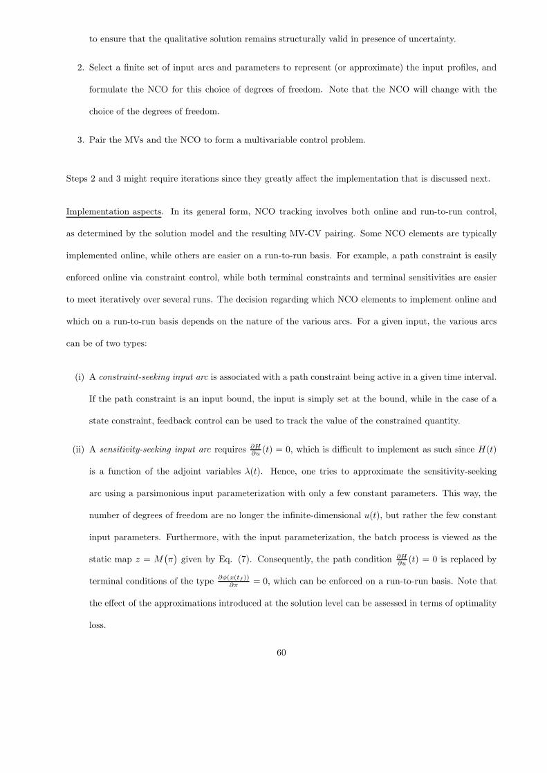
to ensure that the qualitative solution remains structurally valid in presence of uncertainty.

2. Select a finite set of input arcs and parameters to represent (or approximate) the input profiles, and

formulate the NCO for this choice of degrees of freedom. Note that the NCO will change with the

choice of the degrees of freedom.

3. Pair the MVs and the NCO to form a multivariable control problem.

Steps 2 and 3 might require iterations since they greatly affect the implementation that is discussed next.

Implementation aspects. In its general form, NCO tracking involves both online and run-to-run control,

as determined by the solution model and the resulting MV-CV pairing. Some NCO elements are typically

implemented online, while others are easier on a run-to-run basis. For example, a path constraint is easily

enforced online via constraint control, while both terminal constraints and terminal sensitivities are easier

to meet iteratively over several runs. The decision regarding which NCO elements to implement online and

which on a run-to-run basis depends on the nature of the various arcs. For a given input, the various arcs

can be of two types:

(i) A constraint-seeking input arc is associated with a path constraint being active in a given time interval.

If the path constraint is an input bound, the input is simply set at the bound, while in the case of a

state constraint, feedback control can be used to track the value of the constrained quantity.

(ii) A sensitivity-seeking input arc requires ∂H∂u (t) = 0, which is difficult to implement as such since H(t)

is a function of the adjoint variables λ(t). Hence, one tries to approximate the sensitivity-seeking

arc using a parsimonious input parameterization with only a few constant parameters. This way, the

number of degrees of freedom are no longer the infinite-dimensional u(t), but rather the few constant

input parameters. Furthermore, with the input parameterization, the batch process is viewed as the

static map z = M(

π)

given by Eq. (7). Consequently, the path condition ∂H∂u (t) = 0 is replaced by

terminal conditions of the type∂φ(x(tf ))

∂π = 0, which can be enforced on a run-to-run basis. Note that

the effect of the approximations introduced at the solution level can be assessed in terms of optimality

loss.

60

In summary, the ease of implementation and therefore the success of NCO tracking depends on the

quality of the approximations that are introduced to generate the solution model (choice of MVs, correspond-

ing NCO, and pairing MV-NCO). These are true engineering decisions that are made with plant optimality

in mind!

10 Optimization Applications

10.1 Semi-batch Reactor with Safety and Selectivity Constraints

A simple semi-batch reactor with jacket cooling is considered to illustrate the NCO-tracking approach and,

in particular, the generation of alternative solution models72.

10.1.1 Problem formulation

• Reaction system: A+B → C, 2B → D, isothermal, exothermic reactions.

• Objective: Maximize the amount of C at a given final time.

• Manipulated input: Feedrate of B.

• Path constraints: Input bounds; heat-removal constraint expressed as a lower bound on the cooling

jacket temperature.

• Terminal constraint: Upper bound on the amount of D at final time.

61

Model equations. Assuming perfect control of the reactor temperature through adjustment of the cooling

jacket temperature, the model equations read:

˙cA = −k1cAcB −u

VcA, cA(0) = cA,0, (78)

˙cB = −k1cAcB − 2k2c2B +

u

V(cBin

− cB), cB(0) = cB,0, (79)

V = u, V (0) = V0, (80)

Tj = Tr −V

UA

[

(−∆H1)k1cAcB + (−∆H2)k2 c2B

]

, (81)

nC = nA,0 − nA, (82)

nD =1

2

[

(nA − nA,0)− (nB − nB,0) + cBin(V − V0)

]

, (83)

where the number of moles of Species X is defined as nX(t) = V (t) cX(t).

Variables and parameters. cX : concentrations of Species X , nX : number of moles of species X , V : reactor

volume, ki: kinetic coefficient of reaction i, u: feedrate of B, cBin: inlet concentration of B, ∆Hi: enthalpy of

reaction i, Tr: reactor temperature, Tj : cooling jacket temperature, U : heat-transfer coefficient, A: reactor

heat-exchange area. The model, operating and optimization parameters are given in Table 5.

Table 5: Model parameters, operating bounds and initial conditions.

k1 0.11 L/(mol min) k2 0.13 L/(mol min)

∆H1 −8× 104 J/mol ∆H2 −105 J/mol

UA 1.25× 104 J/(min ◦C) cBin5 mol/L

Tr 30 ◦C Tj,min 10 ◦C

umax 1 L/min nD,max 100 mol

cA,0 0.5 mol/L cB,0 0 mol/L

V0 1000 L tf 180 min

62

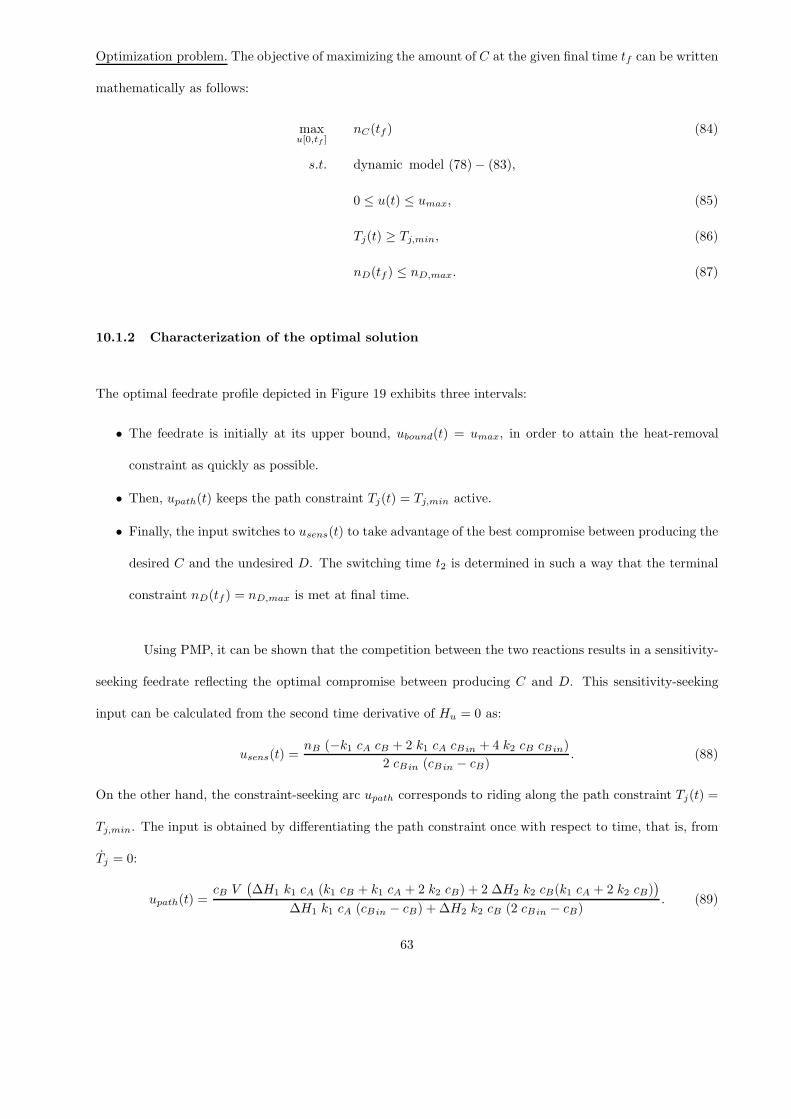
Optimization problem. The objective of maximizing the amount of C at the given final time tf can be written

mathematically as follows:

maxu[0,tf ]

nC(tf ) (84)

s.t. dynamic model (78)− (83),

0 ≤ u(t) ≤ umax, (85)

Tj(t) ≥ Tj,min, (86)

nD(tf ) ≤ nD,max. (87)

10.1.2 Characterization of the optimal solution

The optimal feedrate profile depicted in Figure 19 exhibits three intervals:

• The feedrate is initially at its upper bound, ubound(t) = umax, in order to attain the heat-removal

constraint as quickly as possible.

• Then, upath(t) keeps the path constraint Tj(t) = Tj,min active.

• Finally, the input switches to usens(t) to take advantage of the best compromise between producing the

desired C and the undesired D. The switching time t2 is determined in such a way that the terminal

constraint nD(tf ) = nD,max is met at final time.

Using PMP, it can be shown that the competition between the two reactions results in a sensitivity-

seeking feedrate reflecting the optimal compromise between producing C and D. This sensitivity-seeking

input can be calculated from the second time derivative of Hu = 0 as:

usens(t) =nB (−k1 cA cB + 2 k1 cA cBin + 4 k2 cB cBin)

2 cBin (cBin − cB). (88)

On the other hand, the constraint-seeking arc upath corresponds to riding along the path constraint Tj(t) =

Tj,min. The input is obtained by differentiating the path constraint once with respect to time, that is, from

Tj = 0:

upath(t) =cB V

(

∆H1 k1 cA (k1 cB + k1 cA + 2 k2 cB) + 2 ∆H2 k2 cB(k1 cA + 2 k2 cB))

∆H1 k1 cA (cBin − cB) + ∆H2 k2 cB (2 cBin − cB). (89)

63

0 50 100 150 180

0

0.2

0.4

0.6

0.8

1

time (min)

Fe

ed

rate

(L

/min

)

t t t1 2 f

u [0,t1)

bound

u [t1,t2)path

u [t2,tf]sens

Figure 19: Optimal feedrate consisting of the three arcs ubound[0, t1), upath[t1, t2) and usens[t2, tf ].

Since analytical expressions exist for all three input arcs, and t1 can be determined upon Tj(t)

reaching Tj,min, the optimal solution can be parameterized using a single parameter, namely, the switching

time t2 between upath(t) and usens(t). Note that the input arc upath(t) given by Eq. (89) will keep the

reactor on the path constraint only for the case of a perfect model and perfect measurements. Fortunately,

in the presence of uncertainty, one can implement upath(t) by forcing Tj(t) to track the reference Tj,min,

which is straightforward to implement using, for example, PI control. Similarly, the arc usens(t) is only

optimal for the case of a perfect model and perfect measurements. The way around this difficulty is best

handled with the selection of an appropriate solution model.

10.1.3 Alternative solution models

A key feature of NCO tracking is the possibility to choose appropriate MVs and CVs and, if necessary, to

introduce approximations. Hence, the choice of MVs and CVs is not made once for all, but it may require

iterations. In fact, the appropriateness of these choices is often key to the success of NCO tracking in

practice. This is illustrated next for this example, whereby three alternative solution models are proposed,

all with the same objective but with very different implementation aspects.

64

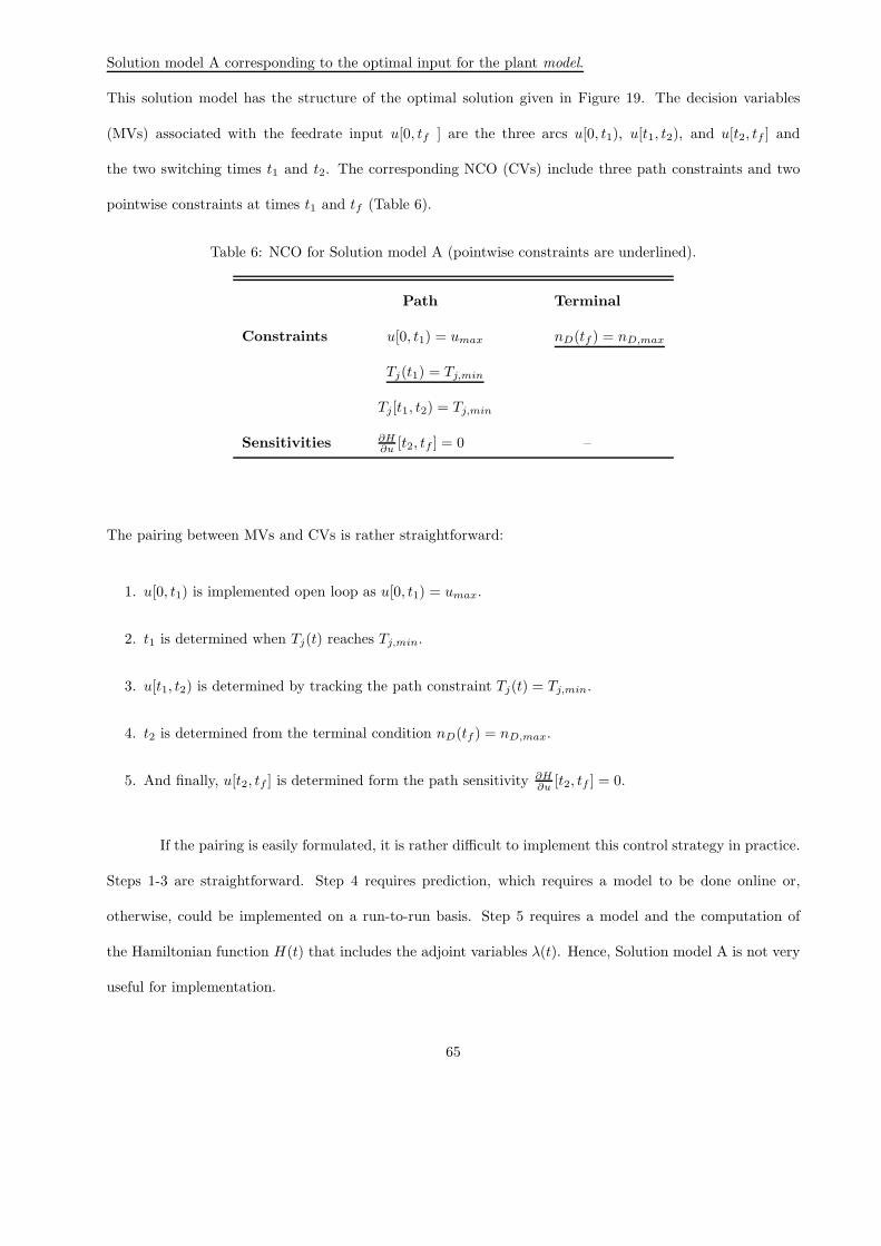
Solution model A corresponding to the optimal input for the plant model.

This solution model has the structure of the optimal solution given in Figure 19. The decision variables

(MVs) associated with the feedrate input u[0, tf ] are the three arcs u[0, t1), u[t1, t2), and u[t2, tf ] and

the two switching times t1 and t2. The corresponding NCO (CVs) include three path constraints and two

pointwise constraints at times t1 and tf (Table 6).

Table 6: NCO for Solution model A (pointwise constraints are underlined).

Path Terminal

Constraints u[0, t1) = umax nD(tf ) = nD,max

Tj(t1) = Tj,min

Tj[t1, t2) = Tj,min

Sensitivities ∂H∂u [t2, tf ] = 0 –

The pairing between MVs and CVs is rather straightforward:

1. u[0, t1) is implemented open loop as u[0, t1) = umax.

2. t1 is determined when Tj(t) reaches Tj,min.

3. u[t1, t2) is determined by tracking the path constraint Tj(t) = Tj,min.

4. t2 is determined from the terminal condition nD(tf ) = nD,max.

5. And finally, u[t2, tf ] is determined form the path sensitivity ∂H∂u [t2, tf ] = 0.

If the pairing is easily formulated, it is rather difficult to implement this control strategy in practice.

Steps 1-3 are straightforward. Step 4 requires prediction, which requires a model to be done online or,

otherwise, could be implemented on a run-to-run basis. Step 5 requires a model and the computation of

the Hamiltonian function H(t) that includes the adjoint variables λ(t). Hence, Solution model A is not very

useful for implementation.

65

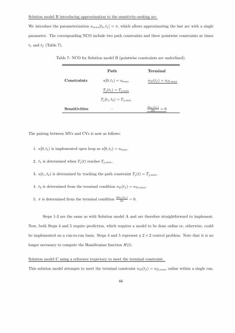
Solution model B introducing approximation to the sensitivity-seeking arc.

We introduce the parameterization usens[t2, tf ] = π, which allows approximating the last arc with a single

parameter. The corresponding NCO include two path constraints and three pointwise constraints at times

t1 and tf (Table 7).

Table 7: NCO for Solution model B (pointwise constraints are underlined).

Path Terminal

Constraints u[0, t1) = umax nD(tf ) = nD,max

Tj(t1) = Tj,min

Tj[t1, t2) = Tj,min

Sensitivities –∂nC(tf )

∂π = 0

The pairing between MVs and CVs is now as follows:

1. u[0, t1) is implemented open loop as u[0, t1) = umax.

2. t1 is determined when Tj(t) reaches Tj,min.

3. u[t1, t2) is determined by tracking the path constraint Tj(t) = Tj,min.

4. t2 is determined from the terminal condition nD(tf ) = nD,max.

5. π is determined from the terminal condition∂nC(tf )

∂π = 0.

Steps 1-3 are the same as with Solution model A and are therefore straightforward to implement.

Now, both Steps 4 and 5 require prediction, which requires a model to be done online or, otherwise, could

be implemented on a run-to-run basis. Steps 4 and 5 represent a 2 × 2 control problem. Note that it is no

longer necessary to compute the Hamiltonian function H(t).

Solution model C using a reference trajectory to meet the terminal constraint.

This solution model attempts to meet the terminal constraint nD(tf ) = nD,max online within a single run.

66

For this, we define the profile nD,term(t) in the time interval [t2, tf ] that has the property to end up at

nD,max at final time. One could, for example, define a profile that increases linearly between nD,2 at t2 and

nD,max at tf :

nD,term(t) = nD,2 +nD,max − nD,2

tf − t2(t− t2). (90)

This way, the corresponding NCO include three path constraints and three pointwise constraints at times t1

and t2 and tf (Table 8).

Table 8: NCO for Solution model C (pointwise constraints are underlined).

Path Terminal

Constraints u[0, t1) = umax –

Tj(t1) = Tj,min

Tj [t1, t2) = Tj,min

nD(t2) = nD,2

nD[t2, tf ] = nD,term[t2, tf ]

Sensitivities –∂nC(tf )∂nD,2

= 0

The pairing between MVs and CVs is now as follows:

1. u[0, t1) is implemented open loop as u[0, t1) = umax.

2. t1 is determined when Tj(t) reaches Tj,min.

3. u[t1, t2) is determined by tracking the path constraint Tj(t) = Tj,min.

4. t2 is determined when nD(t) reaches the predefined value nD,2 for the current batch.

5. u[t2, tf ] is determined by tracking the path constraint nD(t) = nD,term(t).

Again, Steps 1-3 are the same as with Solution models A and B. What is new is that Steps 4 and

5 are now also straightforward to implement online, provided the concentration of the Species D can be

measured or estimated online.

67

A comparison of Tables 6-8 calls for the following comments:

• Solution model A, which is able to generate the numerical solution obtained from the plant model, is

very impractical for implementation using feedback control. However, note that this parameterization

might be rather handy for numerical optimization, for example as an alternative to CVP.

• Solution model B can be implemented via a combination of online and run-to-run control since it does

not contain path sensitivities that typically require a model for computation.

• Solution model C contains mostly path constraints that can be handled via online control. The terminal

sensitivity∂nC(tf )∂nD,2

= 0 is a way of determining the optimal value of nD,2. However, for any practical

purpose, the value of nD,2 can be chosen conservatively (slightly smaller than nD,max) with negligible

effect on the cost.

• All the corresponding tracking schemes attempt to meet the active constraints and push certain gra-

dients to zero. Like with any control scheme, one cannot guarantee, in the presence of disturbances,

that the setpoints are met at all times. However, the presence of feedback helps reduce the sensitivity

to these disturbances. One finds here all the pros and cons of multivariable feedback control!

10.1.4 Simulation results

Optimization results using NCO tracking with the there aforementioned solution models are presented next.

It is assumed that uncertainty is present in the form of time-varying kinetic coefficients for the plant:

k1(t) = k1,0α

α+ t, k2(t) = k2,0

β

α− t, (91)

with the nominal model values k1,0 = 0.11 L/(mol min), k2,0 = 0.13 L/(mol min), α = 1800 min and

β = 900 min, and where t is the time in minutes. These variations might correspond to a change in catalyst

activity with time. The information regarding these variations is, of course, not revealed to the optimization

algorithms. If this information were available, the ideal cost value would be J∗ = 392.3 mol of the desired

product C.

68

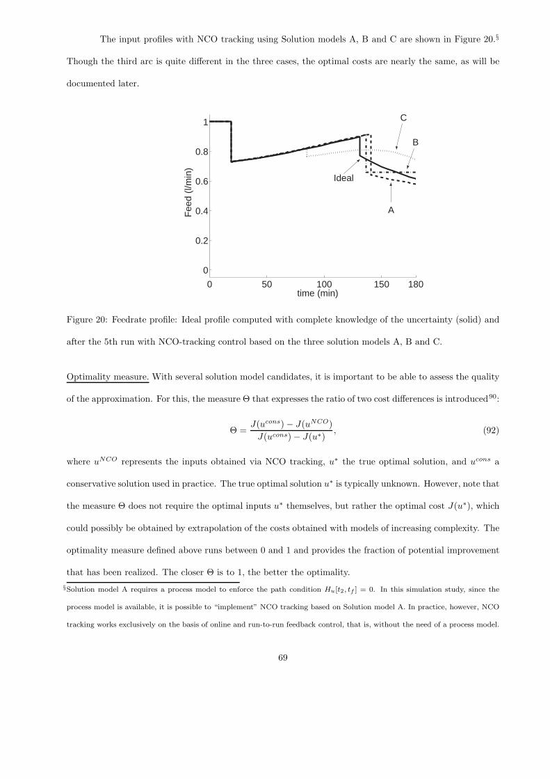
The input profiles with NCO tracking using Solution models A, B and C are shown in Figure 20.§

Though the third arc is quite different in the three cases, the optimal costs are nearly the same, as will be

documented later.

0 50 100 150

0

0.2

0.4

0.6

0.8

1

time (min)

Fee

d (l/

min

)

C

B

Ideal

A

180

Figure 20: Feedrate profile: Ideal profile computed with complete knowledge of the uncertainty (solid) and

after the 5th run with NCO-tracking control based on the three solution models A, B and C.

Optimality measure. With several solution model candidates, it is important to be able to assess the quality

of the approximation. For this, the measure Θ that expresses the ratio of two cost differences is introduced90:

Θ =J(ucons)− J(uNCO)

J(ucons)− J(u∗), (92)

where uNCO represents the inputs obtained via NCO tracking, u∗ the true optimal solution, and ucons a

conservative solution used in practice. The true optimal solution u∗ is typically unknown. However, note that

the measure Θ does not require the optimal inputs u∗ themselves, but rather the optimal cost J(u∗), which

could possibly be obtained by extrapolation of the costs obtained with models of increasing complexity. The

optimality measure defined above runs between 0 and 1 and provides the fraction of potential improvement

that has been realized. The closer Θ is to 1, the better the optimality.

§Solution model A requires a process model to enforce the path condition Hu[t2, tf ] = 0. In this simulation study, since the

process model is available, it is possible to “implement” NCO tracking based on Solution model A. In practice, however, NCO

tracking works exclusively on the basis of online and run-to-run feedback control, that is, without the need of a process model.

69

Quantitative comparaison. The results are compared in Table 9, where, for all cases, convergence is achieved

in less than 10 runs. For the sake of comparison, application of the optimal input calculated offline using

the nominal plant model, ucons, gives the cost J(ucons) = 374.6 mol. The main observations are as follows:

• The constraint on the jacket temperature is active in all cases since it is handled online. The first run

with Controllers A and B indicates how much can be gained by meeting that path constraint alone.

• Enforcing the path sensitivity in Controller A using a model and neighboring-extremal control75 is not

really better (here even slightly worse) than a crude approximation by a constant value as implemented

by Controller B.

• Meeting the terminal constraint improves the cost significantly. This is done via run-to-run control

for Controllers A and B and online via tracking of nD,term(t) in Controller C. Hence, with Controller

C, all the constraints are met online and thus the cost is nearly optimal from the first run on. The

parameter nD,2, which indirectly selects the switching time t2, has a negligible effect on the cost and

therefore is not adapted in this study. ¶ Hence, all the adjustments with Controller C are made online.

10.2 Industrial Batch Polymerization

The last case study illustrates the use of NCO tracking for the optimization of an industrial reactor for the

copolymerization of acrylamide91. As the polymer is repeatedly produced in a batch reactor, run-to-run

NCO tracking using run-end measurements is applied.

10.2.1 A brief description of the process

The 1-ton industrial reactor investigated in this section is dedicated to the inverse-emulsion copolymerization

of acrylamide and quaternary ammonium cationic monomers, a heterogeneous water-in-oil polymerization

¶In this example, the terminal sensitivities are so low that there is no need for adaptation. This is valid for π in Controller B

and nD,2 in Controller C.

70

Run Min. jacket Final amount Final amount Optimality

Controller index temperature of D (mol) of C (mol) measure

Tj,min = 10 ◦C nD,max = 100 mol Cost J Θ

Optimal 10 100 392.3 1

Open loop 10.1 72.5 374.6 0

1 10.0 79.6 376.8 0.12

A 5 10.0 96.2 389.8 0.86

10 10.0 99.6 392.1 0.99

1 10.0 83.6 383.3 0.49

B 5 10.0 98.1 391.6 0.96

10 10.0 99.9 392.2 0.99

1 10.0 100 391.8 0.97

C 5 10.0 100 391.8 0.97

10 10.0 100 391.8 0.97

Table 9: Comparison of NCO-tracking scenarios for three different controllers and various numbers of runs:

Distance to the two constraints, cost J and optimality measure Θ. “Optimal” is with respect to the per-

turbed system. “Open loop” means open-loop application of the optimal input computed for the nominal

(unperturbed) system. Note that open-loop application of the nominal optimal input does not meet the two

constraints and is therefore widely suboptimal.

71

process. Nucleation and polymerization are confined to the aqueous monomer droplets, while the polymer-

ization follows a free-radical mechanism. Table 10 summarizes the reactions that are known to occur.

Table 10: Main reactions in the inverse-emulsion process.

Oil-phase reactions

- initiation by initiator decomposition

- reactions of primary radicals

- propagation reactions

Transfer between phases

- initiator

- co-monomers

- primary radicals

Aqueous-phase reactions

- reactions of primary radicals

- propagation reactions

- unimacromolecular termination with emulsifier

- reactions of emulsifier radicals

- transfer to monomer

- addition to terminal double bond

- termination by disproportionation

A tendency model capable of predicting the conversion and the average molecular weight was de-

veloped. The 7th-order model includes balance equations for the two monomers and for the chain-transfer

agent, dynamic equations for the zeroth-, first- and second-order moments of the molecular weight distribu-

tion and for the efficiency of the initiator. The model parameters have been fitted to match observed data.

Note that certain effect are nearly impossible to model. For instance, the efficiency of the initiator can vary

significantly between batches because of residual oxygen concentration at the outset of the reaction. Chain-

transfer agents and reticulants are also added to help control the molecular weight distribution. These small

72

variations in the recipe are not incorporated in the tendency model. Hence, optimization of this process

clearly calls for the use of measurement-based techniques.

10.2.2 Nominal optimization of the tendency model

The objective is to minimize the reaction time, while meeting four constraints, namely, (i) the terminal

molecular weight X(tf ) has to exceed the target value Xmin to ensure total conversion of acrylamide, (ii)

the terminal conversion Mw(tf ) has to exceed a target value to ensure total conversion of acrylamide, (iii)

heat removal is limited, which is incorporated in the optimization problem by the lower bound Tj,in,min on

the jacket inlet temperature Tj,in(t), and (iv) the reactor temperature Tr(t) is upper bounded. The MVs

are the reactor temperature profile Tr[0, tf ] and the reaction time tf . The dynamic optimization problem

can be formulated as follows:

minTr [0,tf ],tf

J := tf (93)

s.t. dynamic reactor model with initial conditions

X(tf ) ≥ Xmin, (94)

Mw(tf ) ≥ Mw,min, (95)

Tj,in(t) ≥ Tj,in,min, (96)

Tr(t) ≤ Tr,max. (97)

10.2.3 Solution model

The results of nominal optimization are shown in Figure 21, with normalized values of the reactor temperature

Tr(t) and of the time t. The nominal optimal solution consists of two arcs with the following interpretation:

• Heat-removal limitation. Up to a certain level of conversion, the temperature is limited by heat-

removal. Initially, the operation is isothermal and corresponds closely to what is used in industrial

practice. Also, this first isothermal arc ensures that the terminal constraint on molecular weight will

73

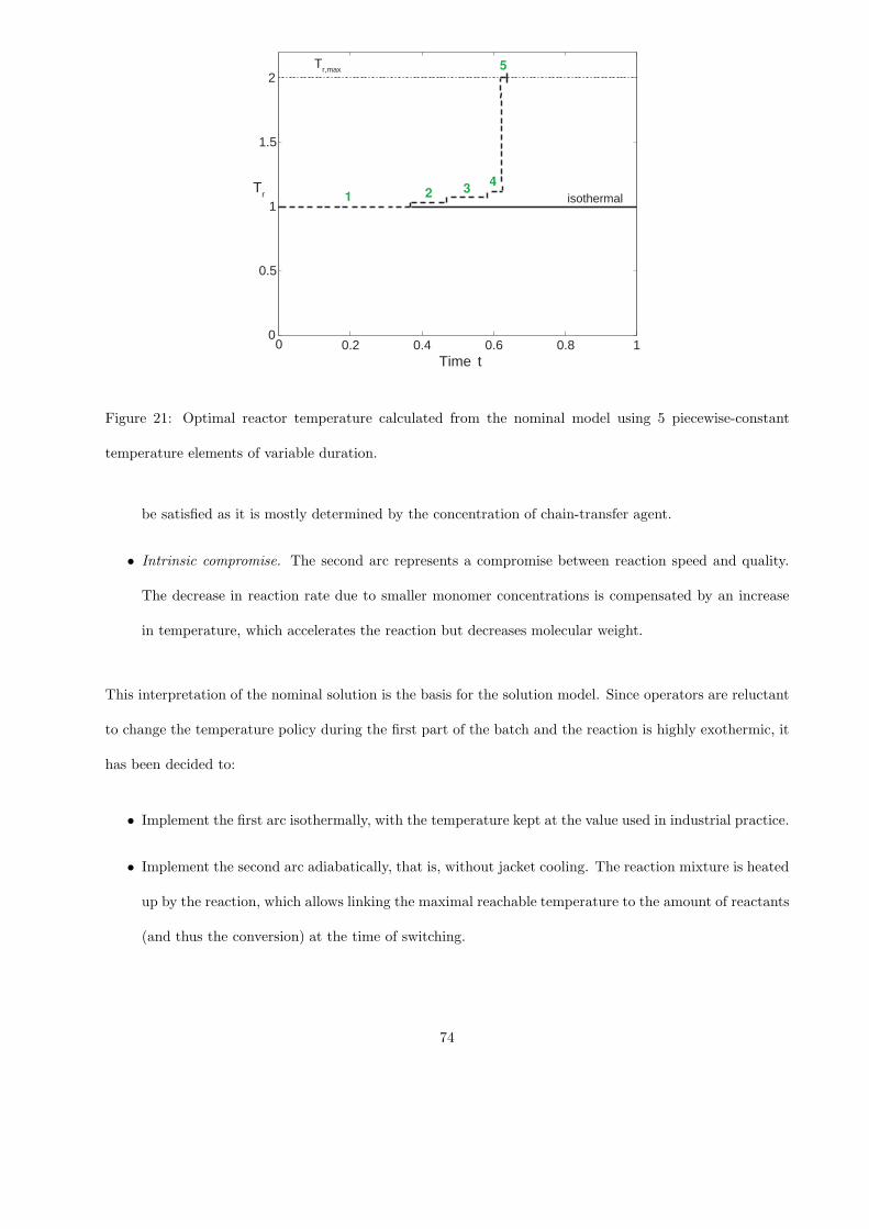
0 0.2 0.4 0.6 0.8 10

0.5

1

1.5

2

Time

Tr

Tr,max

t

5

1 2 34

isothermal

Figure 21: Optimal reactor temperature calculated from the nominal model using 5 piecewise-constant

temperature elements of variable duration.

be satisfied as it is mostly determined by the concentration of chain-transfer agent.

• Intrinsic compromise. The second arc represents a compromise between reaction speed and quality.

The decrease in reaction rate due to smaller monomer concentrations is compensated by an increase

in temperature, which accelerates the reaction but decreases molecular weight.

This interpretation of the nominal solution is the basis for the solution model. Since operators are reluctant

to change the temperature policy during the first part of the batch and the reaction is highly exothermic, it

has been decided to:

• Implement the first arc isothermally, with the temperature kept at the value used in industrial practice.

• Implement the second arc adiabatically, that is, without jacket cooling. The reaction mixture is heated

up by the reaction, which allows linking the maximal reachable temperature to the amount of reactants

(and thus the conversion) at the time of switching.

74

With this so-called semi-adiabatic temperature profile, there are only two degrees of freedom, namely, the

switching time between the two arcs tsw and the final time tf . The dynamic optimization problem can be

rewritten as the following static problem (see Section 8.2):

mintsw, tf

tf (98)

s.t. static model (in this study, the plant)

X(tf) ≥ Xmin, (99)

Mw(tf ) ≥ Mw,min, (100)

Tr(tf ) ≤ Tr,max. (101)

Such a reformulation is made possible since:

a. The switching time tsw and the final time tf are fixed at the beginning of the batch, while performance

and constraints are evaluated at batch end. This way, the dynamics are lumped into the static map

(7) {π : tsw, tf} → {z : tf , X(tf ), Mw(tf ), Tr(tf )}.

b. Maintaining the temperature constant initially at its current practice value ensures that the heat-

removal limitation is satisfied. This constraint can thus be removed from the problem formulation.

Because (i) the constraint on the molecular weight is less restrictive than that on the reactor tem-

perature, (ii) the final time is defined upon meeting the desired conversion, and (iii) the terminal constraint

on reactor temperature is active at the optimum, the NCO reduce to the following two conditions:

Tr(tf )− Tr,max = 0, (102)

∂tf∂tsw

+ ν∂[Tr(tf )− Tr,max]

∂tsw= 0, (103)

where ν is the Lagrange multiplier associated with the constraint on final temperature. The first equation

determines the switching time, while the second equation can be used for computing ν, which however is not

used in this study.

75

10.2.4 Industrial results

The solution to the original dynamic optimization problem can be approximated by adjusting the switching

time so as to meet the terminal constraint on reactor temperature. This can be implemented using a simple

integral run-to-run controller as shown in Figure 22.

Input

GenerationReactor

Disturbances

q j[0,tf]

1

2

Adiabatic

tsI-Controller

-

Tr,maxTr

Run-to-run

(tf)

Isothermal

Figure 22: Run-to-run control of the final reactor temperature by adjusting the switching time ts. The

reactor is initially operated isothermally at the normalized temperature Tr,ref = 1. Adiabatic operation

starts at ts, which is adjusted on a run-to-run basis to achieve Tr(tf ) = Tr,max. The manipulated input is

the flowrate of cooling medium in the jacket qj(t), which is generated by a feedback control law to regulate

Tr(t) around Tr,ref = 1 in the isothermal phase for t < ts; then, qj [ts, tf ] = 0 is set in the adiabatic phase.

Figure 23 depicts the application of the method to the optimization of the 1-ton industrial reactor.

The first batch is performed using a conservative value of the switching time. The reaction time is significantly

reduced after only two batches, without any off-spec product. Table 11 summarizes the adaptation results,

highlighting the 35% reduction in reaction time compared to the isothermal policy used in industrial practice.

Results could have been even more impressive, but a backoff from the constraint on the final temperature

was added for safety purposes. This semi-adiabatic policy has become standard practice for our industrial

partner. The same policy has also been implemented, together with the adaptation scheme, to other polymer

grades and to larger reactors.

76

0 0.2 0.4 0.6 0.8 10

0.5

1

1.5

2

2.5

Tr

Tr,maxr,max

Normalized time

12

3

0

Figure 23: Normalized temperature profiles measured in an industrial reactor as a result of reducing the

switching time between isothermal and adiabatic operations. Compared to the normalized reaction time of

1 for the current-practice isothermal operation, the reaction time is successively reduced to 0.78, 0.72, and

0.65 in 3 batches. Note that a backoff from Tr,max is implemented for safety purposes, mainly to account

for run-time disturbances that cannot be handled by this technique.

Table 11: Run-to-run optimization results for a 1-ton copolymerization reactor.

Batch Strategy tsw Tr(tf ) tf

0 Isothermal 1.00 1.00

1 Semi-adiabatic 0.65 1.70 0.78

2 Semi-adiabatic 0.58 1.78 0.72

3 Semi-adiabatic 0.53 1.85 0.65

77

11 Conclusions

11.1 Summary

This chapter has analyzed the operation of batch and semi-batch processes with respect to both control

and optimization. There often is a great potential for process improvement in batch processes. Although

the major gains are concerned with chemical choices regarding the reaction and separation steps, process

operation also carries a significant potential for cost reduction. However, cost savings in process operations

are often associated with automation rather than advanced control. The former term encompasses the

hardware and software elements needed to operate an industrial process as automatically as possible. These

include automatic start-up and shut-down operations, process monitoring, fault diagnosis, alarm handling,

automatic sampling and analysis. The latter term is concerned mainly with algorithmic solutions for solving

well-defined problems and, as such, might only represent 10% of the control and automation activities in the

batch process industry.

This chapter has also shown that incorporating measurements in the optimization framework helps

improve the performances of chemical processes despite the use of models of limited accuracy. The various

RTO methods differ in the way measurements are used and the inputs are adjusted to reject the effect

of uncertainty. Measurements can be utilized to iteratively (i) update the states or the parameters of the

model that is used for optimization, or (ii) adjust the inputs via feedback control to enforce the NCO. It

has been argued that the latter technique has the ability of rejecting the effect of uncertainty in the form of

plant-model mismatch and process disturbances.

11.2 Future Challenges

While several of the techniques presented here have been implemented successfully in industrial practice,

many challenging problems still remain. Here are a few of them:

78

• Advances in optimization techniques in general, and in model predictive control in particular, have

undoubtedly influenced industrial implementation. However, these techniques depend on the availabil-

ity of process models of reasonably high fidelity and modest complexity, which is difficult to achieve

in practice. Methods of nonlinear model reduction capable of representing complex process dynamics

effectively with reduced-order, control-relevant models will provide a significant boost to the industrial

application of advanced control and optimization techniques.

• While advances in state estimation have enabled the estimation of infrequently measured product char-

acteristics, these estimates can never completely replace the actual measurements themselves. And as

the manufacturing chain becomes inexorably more tightly integrated, each successive downstream cus-

tomer will place increasingly stringent performance demands on the products they receive from each of

their suppliers. Meeting these demands will ultimately require process control performance levels that

cannot be attained without better measurement or estimation of product properties. Advances in sen-

sors, analyzers and ancillary measurement technology will be required in order to make measurements

of product properties more frequently available than is currently possible.

• As the structure of process control systems gets more complex, analyses of model dynamics, overall

system stability and achievable performance will be essential, especially for providing guidance in

selecting the best alternative for each problem.

12 Acknowledegments

The authors would like to thank the former and present group members at EPFL’s Laboratoire d’Automatique,

who contributed many of the insights and results presented here. A particular thank goes to Dr. Alejandro

Marchetti and Dr. Rene Schneider who provided useful feedback on the manuscript.

79

References

1. D. Bonvin. Control and optimization of batch processes. In J. Baillieul and T. Samad, editors, Ency-

clopedia of Systems and Control, pages 1–6. Springer, 2014.

2. D. Bonvin. Optimal operation of batch reactors - A personal view. J. Process Contr., 8(5–6):355–368,

1998.

3. U. Diwekar. Batch Processing: Modeling and Design. CRC Press, 2014.

4. K. Y. Rani. Optimization and Control of Semi-Batch Reactors: Data-Driven Model-Based Approaches.

LAP Lambert Academic Publishing, 2011.

5. F. Caccavale, M. Iamarino, F. Pierri, and V. Tufano. Control and Monitoring of Chemical Batch Reac-

tors. Advances in Industrial Control. Springer-Verlag, New York, 2011.

6. I. M. Mujtaba. Batch Distillation: Design and Operation. Series on Chemical Engineering: Vol. 3.

Imperial College Press, London UK, 2004.

7. U. Diwekar. Batch Distillation: Simulation, Optimal Design, and Control. Series in Chemical and

Mechanical Engineering. CRC Press, 1995.

8. H. Seki, N. Furuya, and S. Hoshino. Evaluation of controlled cooling for seeded batch crystallization

incorporating dissolution. Chem. Eng. Sci., 77(10):10–17, 2012.

9. D. Wieckhusen. Development of batch crystallizations. In W. Beckmann, editor, Crystallization: Basic

Concepts and Industrial Applications, pages 187–202. Wiley-VCH, 2013.

10. L. Ljung. System Identification: Theory for the User. Prentice Hall, 1999.

11. R. K. Pearson and B. A. Ogunnaike. Nonlinear Process Identification. Prentice-Hall, Inc., 1996.

12. D. M. Himmelblau. Applications of artificial neural networks in chemical engineering. Korean Journal

of Chemical Engineering, 17(4):373–392, 2000.

13. S. A. Russel, P. Kesavan, J. H. Lee, and B. A. Ogunnaike. Recursive data-based prediction and control

of batch product quality. AIChE J., 44(11):2442–2458, 1998.

80

14. W. G. Cochran and G. M. Cox. Experimental Designs. John Wiley, 1992.

15. B. Srinivasan and D. Bonvin. Controllability and stability of repetitive batch processes. J. Process

Contr., 17:285–295, 2007.

16. C. Pertev, M. Turker, and R. Berber. Dynamic modelling, sensitivity analysis and parameter estimation

of industrial yeast fermenters. Comp. Chem. Eng., 21:S739–S744, 1997.

17. D. C. Montgomery. Design and Analysis of Experiments. John Wiley & Sons, New York, 8th edition,

2013.

18. S. B. Jorgensen and K. M. Hangos. Grey-box modelling for control: Qualitative models as unifying

framework. Int. J. Adaptive Control and Signal Proc., 9(6):547–562, 1995.

19. H. J. A. F. Tulleken. Application of the grey-box approach to parameter estimation in physico-chemical

models. In IEEE CDC, pages 1177–1183, Brighton, UK, 1991.

20. C. Filippi, J. L. Greffe, J. Bordet, J. Villermaux, J. L. Barnay, B. Ponte, and C. Georgakis. Tendency

modeling of semi-batch reactors for optimization and control. Comp. Chem. Eng., 41:913–920, 1986.

21. G. Francois, B. Srinivasan, and D. Bonvin. Use of measurements for enforcing the necessary conditions

of optimality in the presence of constraints and uncertainty. J. Process Contr., 15(6):701–712, 2005.

22. B. A. Ogunnaike and W. H. Ray. Process Dynamics, Modeling and Control. Oxford University Press,

1994.

23. D. E. Seborg, T. F. Edgar, D. A. Mellichamp, and F. J. Doyle. Process Dynamics and Control. John

Wiley, New York, 2004.

24. K. J. Astrom and B. Wittenmark. Adaptive Control. Addison-Wesley, Reading, Massachusetts, 2nd

edition, 1995.

25. P. Apkarian and R. Adams. Advanced gain-scheduling techniques for uncertain systems. IEEE Trans.

Control System Tech., 6:21–32, 1998.

81

26. V. Hagenmeyer and M. Nohr. Flatness-based two-degree-of-freedom control of industrial semi-batch

reactors using a new observation model for an extended Kalman filter approach. Int. J. of Control,

81(3):428–438, 2008.

27. M. Shahrokhi and M. Ali Fanaei. Nonlinear temperature control of a batch suspension polymerization

reactor. Polymer Engineering and Science, 42(6):1296–1308, 2002.

28. M. Soroush and C. Kravaris. Nonlinear control of a batch polymerization reactor: An experimental

study. AIChE J., 38(9):1429–1448, 1992.

29. M. R. Juba and J. W. Hamer. Progress and challenges in batch process control. In Chemical Process

Control - CPC-III, pages 139–183, Asilomar, CA, 1986.

30. R. A. Wright and C. Kravaris. Nonminimum-phase compensation for nonlinear processes. AIChE J.,

38(1):2640, 1992.

31. Mettler-Toledo. OptiMax Heat-Flow Calorimetry. http://ch.mt.com, 2016.

32. B. Ogunnaike, G. Francois, M. Soroush, and D. Bonvin. Control of polymerization processes. In W. S.

Levine, editor, The Control Handbook – Control System Applications, pages 12.1–12.23. CRC Press,

2011.

33. J. B. Rawlings and D. Q. Mayne. Model Predictive Control: Theory and Design. Nob Hill Pub, 2009.

34. Z. K. Nagy and R. D. Braatz. Robust nonlinear model predictive control of batch processes. AIChE J.,

49(7):1776–1786, 2003.

35. R. G. Brown. Introduction to Random Signal Analysis and Kalman Filtering. John Wiley & Sons, New

York, 1983.

36. E. W. Kamen and J. K. Su. Introduction to Optimal Estimation. Advanced Textbooks in Control and

Signal Processing. Springer Verlag, 1999.

37. J. Valappil and C. Georgakis. Nonlinear model predictive control of end-use properties in batch reactors.

AIChE J., 48(9):2006 – 2021, 2002.

82

38. J. Flores-Cerrillo and J. F. MacGregor. Within-batch and batch-to-batch inferential-adaptive control of

semibatch reactors: A partial least squares approach. Ind. Eng. Chem. Res., 42:3334–3335, 2003.

39. Y. Yabuki and J. F. MacGregor. Product quality control in semi-batch reactors using mid-course cor-

rection policies. Ind. Eng. Chem. Res., 36:1268–1275, 1997.

40. J. Flores-Cerrillo and J. F. MacGregor. Control of batch product quality by trajectory manipulation

using latent variable models. J. Process Contr., 14:539–553, 2004.

41. C. Welz, B. Srinivasan, and D. Bonvin. Measurement-based optimization of batch processes: Meeting

terminal constraints on-line via trajectory following. J. Process Contr., 18(3-4):375–382, 2008.

42. K. L. Moore. Iterative Learning Control for Deterministic Systems. Springer-Verlag, Advances in In-

dustrial Control, London, 1993.

43. S. Arimoto, S. Kawamura, and F. Miyazaki. Bettering operation of robots by learning. J. Robotic Syst.,

1(2):123–140, 1984.

44. J. Wallen, S. Gunnarsson, R. Henriksson, S. Moberg, and M. Norrlof. ILC applied to a flexible two-link

robot model using sensor-fusion-based estimates. In IEEE CDC, pages 458–463, Shanghai, China, 2009.

45. J. H. Lee and K. S. Lee. Iterative learning control applied to batch processes: An overview. Control

Eng. Practice, 15(10):1306–1318, 2007.

46. Y. Wang, F. Gao, and F. J. Doyle. Survey on iterative learning control, repetitive control, and run-to-run

control. J. of Process Contr., 19(10):1589–1600, 2009.

47. S. Arimoto, T. Naniwa, and H. Suzuki. Robustness of P-type learning control with a forgetting factor

for robotic motion. In 29th Conference on Decision and Control, pages 2640–2645, Honolulu, Hawaii,

December 1990.

48. G. Heinzinger, D. Fenwick, B. Paden, and F. Miyazaki. Stability of learning control with disturbances

and uncertain initial conditions. IEEE Trans. Autom. Contr., 37:110–114, 1992.

83

49. C. Welz, B. Srinivasan, and D. Bonvin. Iterative learning control with input shift. In IFAC DYCOPS’7,

Cambridge, MA, 2004.

50. G. Francois, B. Srinivasan, and D. Bonvin. A globally convergent algorithm for the run-to-run control

of systems with sector nonlinearities. Ind. Eng. Chem. Res., 50(3):1410–1418, 2011.

51. J.-J. E. Slotine and W. Li. Applied Nonlinear Control. Prentice-Hall, 1991.

52. W. C. Thompson. Batch process control. In G. K. Mc Millan and D. M. Considine, editors, Pro-

cess/Industrial Instruments and Control Handbook, pages 3.70–3.84. MacGraw-Hill, 1999.

53. T. Hudak. Programmable controllers. In G. K. Mc Millan and D. M. Considine, editors, Pro-

cess/Industrial Instruments and Control Handbook, pages 3.32–3.50. MacGraw-Hill, 1999.

54. R. Netto and A. Bagri. Programmable logic controllers. Int. J. of Computer Applications, 77(11):27–31,

2013.

55. A. G. Marchetti. Modifier-Adaptation Methodology for Real-time Optimization. Doctoral thesis No. 4449,

EPFL Lausanne, Switzerland, 2009.

56. B. Galloway and G. P. Hancke. Introduction to industrial control networks. IEEE Comm. Surveys &

Tutorials, 15(2):860–880, 2013.

57. D. Ruppen, D. Bonvin, and D. W. T. Rippin. Implementation of adaptive optimal operation for a

semi-batch reaction system. Comp. Chem. Eng., 22:185–189, 1998.

58. W. Bequette. Process Dynamics: Modeling, Analysis and Simulation. Prentice Hall, 1998.

59. I. Eckerman. THE BHOPAL SAGA – Causes and Consequences of the World’s Largest Industrial

Disaster. University Press (India) Private Limited, 2005.

60. A. Marchetti, M. Amrhein, B. Chachuat, and D. Bonvin. Scale-up of batch processes via decentralized

control. In IFAC ADCHEM’06, Gramado, Brazil, 2006.

61. C. Welz, B. Srinivasan, and D. Bonvin. Combined online and run-to-run optimization of batch processes

with terminal constraints. In IFAC ADCHEM’04, Hong-Kong, 2004.

84

62. G. Stephanopoulos. Chemical Process Control: An Introduction to Theory and Practice. Prentice-Hall,

1984.

63. G. Francois and D. Bonvin. Measurement-based real-time optimization of chemical processes. In S. Push-

pavanam, editor, Control and Optimisation of Process Systems, volume 44 of Advances in Chemical

Engineering. Elsevier, 2013.

64. O. Rotava and A. C. Zanin. Multivariable control and real-time optimization – An industrial practical

view. Hydrocarbon Process., 84(6):61–71, 2005.

65. S. Boyd and L. Vandenberghe. Convex Optimization. Cambridge University Press, 2004.

66. T. E. Marlin and A. N. Hrymak. Real-time operations optimization of continuous processes. In AIChE

Symposium Series - CPC-V, volume 93, pages 156–164, 1997.

67. Y. Zhang, D. Monder, and J. F. Forbes. Real-time optimization under parametric uncertainty: A

probability constrained approach. J. Process Contr., 12:373–389, 2002.

68. J. F. Forbes, T. E. Marlin, and J. F. MacGregor. Model adequacy requirements for optimizing plant

operations. Comp. Chem. Eng., 18(6):497–510, 1994.

69. A. Marchetti, B. Chachuat, and D. Bonvin. Modifier-adaptation methodology for real-time optimization.

Ind. Eng. Chem. Res., 48(13):6022–6033, 2009.

70. S. Skogestad. Self-optimizing control: The missing link between steady-state optimization and control.

Comp. Chem. Eng., 24:569–575, 2000.

71. K. B. Ariyur and M. Krstic. Real-Time Optimization by Extremum-Seeking Control. John Wiley, New

York, 2003.

72. B. Srinivasan and D. Bonvin. Real-time optimization of batch processes via tracking the necessary

conditions of optimality. Ind. Eng. Chem. Res., 46(2):492–504, 2007.

73. B. Srinivasan, S. Palanki, and D. Bonvin. Dynamic optimization of batch processes: I. Characterization

of the nominal solution. Comp. Chem. Eng., 44:1–26, 2003.

85

74. L. T. Biegler. Nonlinear Programming: Concepts, Algorithms, and Applications to Chemical Processes.

MOS-SIAM Series on Optimization, 2010.

75. A. E. Bryson and Y. C. Ho. Applied Optimal Control. Hemisphere, Washington DC, 1975.

76. V. S. Vassiliadis, R. W. H. Sargent, and C. C. Pantelides. Solution of a class of multistage dynamic

optimization problems. 1. Problems without path constraints. Ind. Eng. Chem. Res., 33(9):2111–2122,

1994.

77. J. S. Logsdon and L. T. Biegler. Accurate solution of differential-algebraic optimization problems. Ind.

Eng. Chem. Res., 28(11):1628–1639, 1989.

78. A. E. Bryson. Dynamic Optimization. Addison-Wesley, Menlo Park, California, 1999.

79. M. S. Bazarra, H. D. Sherali, and C. M. Shetty. Nonlinear Programming: Theory and Algorithms. John

Wiley and Sons, 2nd edition, New York, USA, 1993.

80. P. E. Gill, W. Murray, and M. H. Wright. Practical Optimization. Academic Press, London, 1981.

81. A. Forsgren, P. E. Gill, and M. H. Wright. Interior-point methods for nonlinear optimization. SIAM

Rev., 44(4):525–597, 2002.

82. B. Srinivasan, L. T. Biegler, and D. Bonvin. Tracking the necessary conditions of optimality with

changing set of active constraints using a barrier-penalty function. Comp. Chem. Eng., 32(3):572–579,

2008.

83. C. K. Chui and G. Chen. Kalman Filtering with Real-Time Applications. Springer Verlag, 4th edition,

2009.

84. J. B. Rawlings. Moving horizon estimation. In J. Baillieul and T. Samad, editors, Encyclopedia of

Systems and Control, pages 1–7. Springer, 2014.

85. D. J. Kozub and J. F. MacGregor. State estimation for semi-batch polymerization reactors. Chem. Eng.

Sci., 47:1047–1062, 1992.

86

86. D. Dochain. State and parameter estimation in chemical and biochemical processes: A tutorial. J.

Process Contr., 13(8):801–818, 2003.

87. B. Wittenmark. Adaptive dual control methods: An overview. In IFAC Symp. on Adaptive Syst. in

Control and Signal Proc., pages 67–72, Budapest, 1995.

88. D. Angeli. Economic model predictive control. In J. Baillieul and T. Samad, editors, Encyclopedia of

Systems and Control, pages 1–9. Springer, 2014.

89. A. G. Marchetti, B. Chachuat, and D. Bonvin. A dual modifier-adaptation approach for real-time

optimization. J. Process Contr., 20(9):1027–1037, 2010.

90. C. Welz, A. G. Marchetti, B. Srinivasan, D. Bonvin, and N. L. Ricker. Validation of a solution model

for the optimization of a batch distillation column. In American Control Conference, Portland, Oregon,

2005.

91. G. Francois, B. Srinivasan, D. Bonvin, J. Hernandez Barajas, and D. Hunkeler. Run-to-run adaptation

of a semi-adiabatic policy for the optimization of an industrial batch polymerization process. Ind. Eng.

Chem. Res., 43(23):7238–7242, 2004.

87