Contracting Frictions with Managers, FinancialFrictions, and Misallocation∗

(Preliminary and Incomplete)

Chaoran ChenNational University of Singapore

Ashique HabibInternational Monetary Fund

Xiaodong ZhuUniversity of Toronto

February 16, 2018

Abstract

Weak contract enforcement prevents productive firms from hiring outside managers andexpanding production in developing countries. We develop a model where firms can increasetheir span of control by hiring outside managers, but weak contract enforcement distortsthis delegation decision since managers can then steal the firm’s output unless properlyincentivized. Firms overcome this friction by hiring fewer managers and increasing thecompensation to managers, which manifests as output wedges at the firm level. We showthat these features are consistent with cross-country evidence from the IPUMS-Internationaldata: The employment share and the wage premium of managers relative to workers arecorrelated with a country’s level of development. In our model, the distortionary effects areincreasing in firm productivity, a necessary property any mechanism needs to generate largelosses due to misallocation. We then further introduce financial frictions into our modeland estimate this model using the firm-level data from China. We find that our model canaccount for the fact that larger firms have a higher marginal product than smaller firms, afeature of the data that standard models of financial frictions alone cannot generate. Wefurther show that the contracting frictions generate larger productivity loss than financialfrictions.

Keywords: Contract Enforcement, Delegation, Financial Frictions, Firm Dynamics, Misal-location, Aggregate Productivity.JEL classification: E13, L16, L26, O41.

∗We thank Diego Restuccia, Daniel Yi Xu, as well as seminar participants at Midwest Macro conferenceat Pittsburgh and Fudan University for helpful comments. All errors are our own. The views expressed hereare those of the authors and should not be attributed to the International Monetary Fund, its ExecutiveBoard, or its management. Contact: Chen: Department of Economics, National University of Singapore,1 Arts Link, AS2 #04-38, Singapore 117568, ecscc@nus.edu.sg. Habib: International Monetary Fund, 70019th Street NW, Washington DC 20431, ahabib@imf.org. Zhu: Department of Economics, University ofToronto, 150 St. George Street, Toronto, Ontario, Canada, M5S 3G7, xzhu@chass.utoronto.ca. This draft ispreliminary and please do not circulate without permission.

1

1 Introduction

Cross-country income differences are largely explained by differences in total factor produc-

tivity (TFP) (Caselli, 2005). A recent literature argues that lower TFP in poor countries can

be accounted for by severe resource misallocation, especially financial constraints on firms. A

common feature of this literature is that financial frictions, often modelled as collateral con-

straints a la Buera et al. (2011) and Moll (2014), mainly affect small firms, while large firms

are less affected. This feature is inconsistent with firm-level data from developing countries

that large firms may potentially face more severe distortions.1 In this paper, we propose that

contracting frictions between firms and outside managers causes significant misallocation by

distorting the delegation decisions of large firms. We document evidence consistent with the

idea that large firms are particularly distorted, and that contracting frictions with outside

managers are particularly worse in developing countries. We then develop a model with

both financial and managerial frictions, and quantitatively show how managerial frictions

are important for both generating large productivity losses and for matching the documented

relationship between firm size and marginal productivity.

Larger firms have higher marginal product of capital, as documented in Hsieh and Olken

(2014). However, models with just financial frictions generate larger distortions for smaller

firms. We first decompose the dispersion of marginal product of capital into the dispersions

of capital labor ratio and marginal product of labor. The dispersion in marginal product

of capital indicates frictions in the capital market, while the latter indicate some other

frictions since financial frictions do not distort the choice of labor. We argue that higher

marginal product of labor of larger firms can be explained by contracting frictions, which

results in lacks of delegation to outside managers. We further use household survey data

from the Integrated Public Use Microdata Series (IPUMS) to document two stylized facts.

The fraction of population working as managers increases with a country’s GDP per capita,

and managers are paid a relatively higher wage premium (efficiency wage) in poor countries

with weak contracting enforcement after controlling for observed characteristics. These two

stylized facts serve as direct evidence for our modelling of contracting frictions.

1For example, Hsieh and Olken (2014) find that large firms have higher marginal products of capital andlabor than small firms using micro data from India, Mexico, and Indonesia.

2

We build our model on Garicano and Rossi-Hansberg (2006), Grobovsek (2017) and

Buera et al. (2011). In our framework, firms face endogenous collateral constraints as well

as contracting frictions with managers. Entrepreneurs can increase their span of control

by hiring outside managers and selecting the number of managerial layers. However, weak

contract enforcement distorts these delegation decisions. Managers can steal firm’s output

when contract enforcement is weak. Firms overcome this friction by hiring fewer managers

and increasing the compensation to managers, consistent with our two stylized facts. Larger

firms benefit more from outside managers than smaller firms, which is why larger firms

are more severely affected by the contracting friction. These larger firms face higher output

wedges which generates a positive relationship between marginal product and size, consistent

with the data.

We calibrate our benchmark economy without financial frictions to U.S. data. Then we

vary the level of both frictions to study the impact on aggregate productivity. Productivity

falls monotonically with both frictions. Whereas financial frictions disproportionately affect

smaller firms, managerial frictions mainly affect large firms. TFP falls by 24% when man-

agerial frictions completely shut down delegation. Contracting frictions have larger impacts

on TFP than financial frictions because contracting frictions distort the larger firms who

produce most of the output in the economy.

Our paper mainly contributes to the macro literature on the importance of firm manage-

ment.2 We build on the framework of Grobovsek (2017), showing how managerial frictions

can help account for observed patterns of factor misallocation.

Our paper is also related to the recent macroeconomic literature on the firm size dis-

tribution and firm dynamics, and their relationship to economic development.3 The closest

related paper is Akcigit et al. (2017), who also argue that the lack of delegation explains

why firms in poor countries have lower productivity and do not grow over their life cycles.

Whereas their paper highlights the importance of selection, we completely shut down this

channel in our model. We highlight the importance of contracting frictions with managers

2See, for example, Garicano and Rossi-Hansberg (2006), Bloom and Reenen (2007), Bloom and Reenen(2010), and Grobovsek (2017), among others.

3See, for example, Haltiwanger et al. (2013), Roys and Seshadri (2014), Hsieh and Klenow (2014), andAkcigit et al. (2017), among others.

3

generate productivity losses by misallocating factors of production, something they abstract

from in their paper.

Our paper also contributes to the misallocation literature by building a framework to

quantify the importance of contracting frictions and lack of delegation.4 The contracting

frictions with managers leads to endogenous output wedges that are positively correlated

with firm productivity. Our work is also related to the literature studying the role of weak

institutions as key obstacles of economic development. Weak contract enforcement is an

often-cited result of weak institutions in poor countries.5

The paper proceeds as follows. Section 2 documents stylized facts both across firms in

China and India and across countries. Section 3 describes our model. We quantify the

impact of the two types of frictions in Section 4. Section 5 concludes the paper.

2 Evidence

In this section we document evidence on contracting frictions both across countries and

across firms.

2.1 Firm-Level Evidence from China and India

2.1.1 A Simple Accounting Framework

We start by documenting firm-level evidence using data from the manufacturing sector of

China and India. To guide our analysis, let us first consider a simple accounting framework.

The profit maximization problem of firm i in industry j is given by

πij = τ yijpiyij − τ kijrkij − wlij.

πij denotes for the profit of this firm. yij, kij, and lij are the firm’s output, capital input,

and labor input, respectively. pi is the price of output, which is constant for industry i. τ yi,j

4For the misallocation literature, see, for example, Restuccia and Rogerson (2008), Hsieh and Klenow(2009), Buera et al. (2011), Moll (2014), and Bento and Restuccia (2017), among others.

5For the literature on institutions and economic growth, see Alchian and Demsetz (1973) and Acemogluet al. (2005) among others.

4

and τ kij are output and capital wedges.6 We further assume that the production function is

Cobb-Douglas: yij = z1−γij (kαijl

1−αij )γ. Then the first order conditions are

αγτ yijpiyijkij

= τ kijr and (1− α)γτ yijpiyijlij

= w. (1)

Definepiyijkij

andpiyijlij

as the revenue productivity of capital and labor (APKij and APLij).

We can rewrite Equation 1 as

APKij ∝τ kijτ yij

and APLij ∝1

τ yij. (2)

The capital-labor ratio (KOLij) of the firm can be written as

kijlij

=α

1− αw

τ kijr∝ 1/τ yij.

We can then show that APKij can be decomposed into APLij and the capital-labor ratio

(KOLij):

APKij = APLij ·1

KOLij. (3)

Intuitively, Equation (3) simply states that the average product of capital can be decomposed

into two terms: the average product of labor which only depends on the output wedge but

not the capital wedge, and the capital-labor ratio which only depends on the capital wedge

but not the output wedge. This decomposition helps us to identify the capital wedges relative

to the output wedges in our firm level data.

2.1.2 Firm-Level Data of China and India

We now document stylized facts in the firm-level data of China and India, where the data

cleaning process follows closely Hsieh and Klenow (2009). Literature typically focuses on

the differences in average product of capital (APK) across firms as evidence for capital

misallocation. Figure 1 shows the APK across firms in the Indian data. We plot firms by

their size (measured as the labor input) on the horizontal axis and plot their APK on the

6Note that it is equivalent to model the capital wedge and labor wedge without the output wedge, butwe cannot have all three wedges in this framework.

5

Figure 1: Average Product of Capital of Indian Firms

-1-.5

0.5

1Av

erag

e Pr

oduc

t of C

apita

l (Lo

g)

0 2 4 6 8Firm Size (Log Labor)

Note: The figure shows the average product of capital across firms of the Indian data in the year 1998. Wecontrol on the firm’s age, ownership, location, and 2-digit industry and then use the residuals of APK toobtain the results in the figure. The data cleaning process is detailed in Appendix A. The dashed lines showthe 95 percent confidence interval.

vertical axis. In general, larger firms have higher APK, consistent with Hsieh and Olken

(2014). In fact suggests that collateral constraints are now likely to explain the dispersion

of APK across firms, since standard models of borrowing constraints typically predict that

small firms are constraint due to a lack of collateral and therefore have higher APK.

In order to study why large firms have higher APK than small firms, we decompose the

APK into the average product of labor (APL) and the capital-labor ratio (KOL) following

Equation (3). The results are in Figure 2. The left panel of Figure 2 shows the KOL across

firms, where the dispersion arises from the capital wedges only. It is clear that there are

severe capital misallocation across firms: larger firms do have higher capital-labor ratio than

smaller firms, consistent with the story of collateral constraint, except for those very small

firms. The right panel of Figure 2 shows the APL across firms, where the dispersion arises

from the output wedges only. It is clear that larger firms have higher APL, consistent with

Hsieh and Olken (2014). This indicates that larger firms face higher output wedges than

smaller firms, and we need to find explanations different from financial frictions to explain

this pattern that APL increases with firm size. As we will show later, our model predicts

that the contracting frictions between entrepreneurs and managers exactly work as output

wedges across firms, and our model also predicts that APL should increases with firm size

when the contract enforcement is week, consistent with these firm-level data.

6

Figure 2: Decomposition of Wedges of Indian Firms

-1-.5

0.5

1C

apita

l-Lab

or R

atio

(Log

)

0 2 4 6 8Firm Size (Log Labor)

-1-.5

0.5

1Av

erag

e Pr

oduc

t of L

abor

(Log

)

0 2 4 6 8Firm Size (Log Labor)

Note: The left figure shows the capital-labor ratio across firms of the Indian data in the year 1998. The rightfigure shows the average product of labor across firms. We control on the firm’s age, ownership, location,and 2-digit industry and then use the residuals to obtain the results in the figure. The data cleaning processis detailed in Appendix A. The dashed lines show the 95 percent confidence interval.

We also present our results using the firm-level data from China in the year of 2004.

The China data are different from the Indian data since the Chinese manufacturing survey

only records firms whose gross output in the previous year is greater than five million RMB

(roughly 750,000 U.S. dollar in the year 2004). This criterion generates selection effect that

biases upward the estimated productivity of small firms: a small firm with only ten workers

will have to be extremely productive to produce five million RMB and to be included in the

survey, while a large firm with 100 workers is able to produce five million RMB and to be

included in the survey even if it is not very productive. Therefore, we mainly discuss on the

pattern among large firms for the China data.

Figure 3 shows the APK across firms in China. Larger firms have lower APK than smaller

firms. Again this pattern depends on both capital wedges and output wedges, therefore we

apply Equation (3) and decompose the pattern into KOL and APL across firms in Figure 4.

If we focus only on large firms, we can see that the KOL increases with firm size, consistent

with the idea that smaller firms face collateral constraints and have lower capital intensity.

Therefore, there are also substantial capital misallocation in China, similar to what we find

in the Indian data. The right panel of Figure 4 shows that the APL increases with firm size,

in a pattern similar to the Indian data as well. Larger firms in China also face higher output

wedges that do not arise from capital frictions. This fact is also consistent with our model

7

Figure 3: Average Product of Capital of Chinese Firms

-.50

.5Av

erag

e Pr

oduc

t of C

apita

l (Lo

g)

2 4 6 8Firm Size (Log Labor)

Note: The figure shows the average product of capital across firms of the China data in the year 2004. Wecontrol on the firm’s age, ownership (especially whether this firm is a state-owned enterprise), location, and2-digit industry and then use the residuals of APK to obtain the results in the figure. The data cleaningprocess is detailed in Appendix A. The dashed lines show the 95 percent confidence interval.

that larger firms are constraint by a lack of delegation to outside managers and therefore

have higher output wedges.

It is important to highlight the issue of selection in the China data. As is mentioned

before, the criterion for a firm to be in the survey is that its gross output of the previous

year is greater than five million RMB. A way to avoid the selection bias is to define firm

size in gross output instead of labor. Figure 5 shows the same decomposition when firm size

is measured by sales (which are closely related to gross output). We can see that both the

capital-labor ratio and the labor productivity are (almost) monotonically increasing in firm

size, confirming our findings in the Indian data that smaller firms face higher capital wedges,

while larger firms face higher output wedges. We further note that we do observe labor

quality differences across firms: the data report the composition of workers with different

education levels. The increasing pattern of APL is robust to controlling for these labor

quality differences.

To conclude, firm-level data from both China and India suggest that large firms face

substantially higher output wedges, which do not arise from capital frictions. The increasing

pattern of APL is consistent with our conjecture that large firms are constraint by lacking

delegation to outside managers due to weak contract enforcement. The following section

uses cross-country evidence to show that the lack of delegation is indeed a problem for many

8

Figure 4: Decomposition of Wedges of Chinese Firms-.5

0.5

Cap

ital-L

abor

Rat

io (L

og)

2 4 6 8Firm Size (Log Labor)

-.50

.5Av

erag

e Pr

oduc

t of L

abor

(Log

)

2 4 6 8Firm Size (Log Labor)

Note: The left figure shows the capital-labor ratio across firms of the China data in the year 2004. The rightfigure shows the average product of labor across firms. We control on the firm’s age, ownership (especiallywhether this firm is a state-owned enterprise), location, and 2-digit industry and then use the residuals ofAPK to obtain the results in the figure. The data cleaning process is detailed in Appendix A. The dashedlines show the 95 percent confidence interval.

Figure 5: Decomposition of Wedges of Chinese Firms: Alternative Size Measure

-10

1C

apita

l-Lab

or R

atio

(Log

)

8 10 12 14Firm Size (Log Sales)

-10

1Av

erag

e Pr

oduc

t of L

abor

(Log

)

8 10 12 14Firm Size (Log Sales)

Note: The left figure shows the capital-labor ratio across firms of the China data in the year 2004. The rightfigure shows the average product of labor across firms. We control on the firm’s age, ownership (especiallywhether this firm is a state-owned enterprise), location, and 2-digit industry and then use the residuals ofAPK to obtain the results in the figure. The data cleaning process is detailed in Appendix A. The dashedlines show the 95 percent confidence interval. These two figures differ from Figure 4 since firm size ismeasured by sales instead of labor input.

9

Figure 6: Fraction of Individuals Working as Managers

ARGARM

AUT

BLR

VEN

BRA

KHM

CAN

CHL

CUB

DOMECU

EGY

SLV

FJI

FRA

GHA

GRC

GINHTI

HUN

IND

ISRJAM

JOR

KGZ

MWIMLI

MEX

MNG

MARMOZ NGA

PAN

PER

PRT PRI

ROU

RWASEN

ESP

SDN

CHE

TZA TUR

USA

URY

VEN

ZMB

0.0

5.1

.15

Man

ager

s (P

erce

ntag

e)

7 8 9 10 11GDP per Capita, PPP (Log)

Note: The figure shows the correlation between the percentages of individuals working as managers and thecountry’s GDP per capita (PPP adjusted). There are 49 observations in the figure. Poor countries in generalhave lower portions of individuals working as managers. The regression coefficient is 0.026, significant at theone percent level, and R2 is 0.47.

poor countries.

2.2 Cross-Country Differences in Contracting Frictions

We document two stylized facts on cross-country differences in contracting frictions. The first

stylized fact is that the fraction of individuals working as managers increases in a country’s

GDP per capita. Figure 6 plots this stylized facts, with log GDP per capita (PPP adjusted)

on the horizontal axis and the fraction of individuals working as managers on the vertical

axis. The data are from the Integrated Public Use Microdata Series, International: Version

6.5 (IPUMS), and see Appendix A for details. Rich countries, such as the United States

and Canada, have around 10 percent of individuals working as managers. In contrast, in

poor countries very few individuals work as managers. The slope is statistically significant

at the one percent level. This stylized fact is consistent with Akcigit et al. (2017), who also

find that firms in poor countries tend to delegate less frequently and this lack of delegation

explains that why firms in poor countries grow slower over time (Hsieh and Klenow, 2014).

The second stylized fact is that managers tend to earn higher income than individuals of

10

Figure 7: Income Premium of Managers

ARG

ARMAUT

BLR

VEN

BRA

KHM

CHL

CUB

DOM

ECU

EGY

SLV

FJI

FRA

GHA

GRC

GIN

HTI

HUN

ISR

JAMJOR

KGZ

MWI

MLI

MEX

MNGMAR

MOZ

NGA

PAN

PER

PRTPRI

ROU

RWA

SEN ESPCHETUR USA

URY

VENZMB

-.20

.2.4

.6.8

Man

ager

Inco

me

Prem

ium

(Log

)

7 8 9 10 11GDP per Capita, PPP (Log)

Note: The figure shows the income differences between managers and individuals of other occupationsversus the country’s GDP per capita (PPP adjusted). There are 45 observations in the figure. The incomedifferences of managers are larger in poor countries. The regression coefficient is -0.078, significant at theone percent level, and R2 is 0.21.

other occupations, and the difference is larger in poor countries than in rich countries. In the

IPUMS-International data, we observe individual’s income for only a few countries, but we

do have information on individual’s consumption, such as the number of rooms, for a large

set of countries. We therefore use the number of rooms of individuals as an approximation of

income. Before we compare income among individuals of different occupations, we first run

the standard Mincer regression to control for observed characteristics, such as education level,

age, and gender. Given the fact that the number of rooms may be affected by the number of

people living in a same home, we further control for the family size in the regression. We then

obtain the residuals from the regression and use them to calculate the income premium of

managers, defined as the room number differences between managers and individuals of other

occupations, for each country. We then correlate this income premium of managers versus

a country’s log GDP per capita. The results are shown in Figure 7. Among 45 countries

that we have data, poor countries in general have larger manager income premiums than

rich countries. The slope is statistically significant at the one percent level.

Note that we have controlled for observed heterogeneity among individuals in the Mincer

11

regression, such as age, gender, and education, and only use the residuals to calculate this

income premium of managers. Therefore, higher manager income premium in poor coun-

tries should not arises from these observed heterogeneity, such as education gaps between

managers and individuals of other occupations. Rather, it may reflect contracting frictions

between entrepreneurs and managers, which result in efficiency wages paid to managers in

poor countries.

To conclude, we find that poor countries have smaller portions of individuals working

as managers, but the income premium of managers are higher in poor countries than in

rich countries. This is consistent with our conjecture that weak contract enforcement in

poor countries result in lacking delegation to outside managers and higher compensation to

managers (as efficiency wages). In the next section, we formally describe our model and

show how our model with contracting frictions generates these two patterns.

3 Model

This model builds on Garicano and Rossi-Hansberg (2006) and Grobovsek (2017). As in

Grobovsek (2017), entrepreneurs can increase their span of control by hiring outside man-

agers, potentially employed in multiple layers. If contract enforcement is not perfect, outside

managers can get away with stealing a fraction of the output that passes through their hands,

which reduces the gains from delegation. We also introduce financial frictions a la Moll (2014)

to this framework in a stylized way, which is potentially important in generating the observed

pattern of marginal products across firms. To integrate these two frameworks, we make sev-

eral simplification assumptions to keep our model tractable. We abstract from entry into

entrepreneurship and therefore we focus on the misallocation along intensive margin rather

than selection. We further restrict managers and entrepreneurs to short-term contracts.

3.1 Households

The economy consists of two types of infinitely-lived households: worker households and

entrepreneurial households.

12

Workers. There are a measure Nw of worker households. Each of these households consist

of a measure 1 of members. In each period, each member has one unit of time that they can

supply directly to firms as unskilled labor, or supply to firms as skilled labor after paying a

training cost κ. The wage for skilled and unskilled labor are ws and wu, respectively. House-

holds pool their members’ incomes and allocate consumption across members to maximize

the household’s utility.

Denote Ns and Nu as the measure of skilled and unskilled labor. The worker household’s

problem is therefore to maximize Ns(ws − κ) + Nuwu, subject to Ns + Nu = Nw. In the

equilibrium, it has to be that ws = wu + κ in order to have positive measures of both types

of labor.

Entrepreneurs. There are a measure Ne of infinitely lived entrepreneurs. Each en-

trepreneur has a production technology that only they can operate. Entrepreneurs differ

in their productivity z, which has a cumulative distribution Fz : R+ 7→ [0, 1].

Entrepreneurs also differ in their exogenous borrowing limit k, which has a cumulative

distribution Fk : R+ 7→ [0, 1]. We model financial frictions in this reduced form and abstract

from the endogenous borrowing limit arising from collateral constraints, since our work

focus more on the contracting frictions between managers and entrepreneurs. Note that this

assumption does not affect our quantitative results on misallocation since we calibrate the

exogenous distribution of the borrowing limit to firm-level data.

An entrepreneur who begins the period with exogenous borrowing limit k and productiv-

ity z earns profit π(k, z) from operating his firm. We will describe shortly how profit π(k, z)

is determined. Entrepreneurs then consume their profit income.

3.2 Production technology

The production technology takes in labor and capital as variable inputs to produce output.

There are five distinct types of labor inputs: the entrepreneur’s, skilled/unskilled production

workers’, and skilled/unskilled managerial workers’. Production workers and managerial

workers need to be supervised, while the entrepreneur uses his one unit of time to supervise

13

either production or managerial workers. Managerial workers can supervise other workers.7

Two-layer firm. The simplest firm consists of an entrepreneur (in layer 2) supervising

capital and production workers (in layer 1). The efficiency of the inputs in layer 1 depends

on the amount of time the entrepreneur spends supervising them. If a firm employs k(1)

units of capital, ms(1) units of skilled production workers, and mu(1) units of unskilled

production workers, then the efficiency per unit of composite input is:

(1

k(1)α (ms(1)1−µmu(1)µ)1−α

)θ, α, µ, θ ∈ (0, 1). (4)

The parameter θ captures the idea that the entrepreneur’s marginal efficiency is decreasing

in the amount of inputs he manages, α governs the capital share, and µ determines the

relative importance between skilled and unskilled workers. The effective units of inputs are

(1

k(1)α (ms(1)1−µmu(1)µ)1−α

)θ×(k(1)α

(ms(1)1−µmu(1)µ

)1−α)

=(k(1)α

(ms(1)1−µmu(1)µ

)1−α)1−θ

.

If the entrepreneur has productivity z, then his total output is;

z(k(1)α

(ms(1)1−µmu(1)µ

)1−α)1−θ

.

Notice that this is a standard decreasing returns to scale technology as Lucas (1978), with

an entrepreneurial profit share of θ.

Three-layer firm. The entrepreneur can increase the amount of supervision received by

the production workers by adding a managerial layer and staffing it appropriately. Manage-

rial inputs also need supervision. Suppose the entrepreneur employs (k(2),ms(2),mu(2) units

of capital, skilled labor, and unskilled labor in the managerial layer and (k(1),ms(1),mu(1)

units of capital, skilled labor, and unskilled labor in the production layer. The effective units

7Grobovsek (2017) considers a model with only labor inputs, where managers use only their time tosupervise. Since we introduce capital as a factor of input, we assume managers use both their time andcapital to supervise the layer below them. This assumption keeps the capital-labor ratio constant acrossfirms in our model.

14

of managerial inputs is

(1

k(2)α (ms(2)1−µγmu(2)µγ)1−α

)θ×((ms(2)1−µγmu(2)µγ

)1−α)

=((ms(2)1−µγmu(2)µγ

)1−α)1−θ

.

The parameter γ < 1 indicates that the managerial layer is more skilled-labor intensive than

the production layer.

The effective units of managerial inputs are used to supervise the inputs in the production

layer. The effective units of production inputs is

(k(2)α (ms(2)1−µγmu(2)µγ)

1−α)1−θ

k(1)α (ms(1)1−µmu(1)µ)1−α

θ

×(k(1)α

(ms(1)1−µmu(1)µ

)1−α)

=(k(2)α

(ms(2)1−µγmu(2)µγ

)1−α)θ(1−θ) (

k(1)α(ms(1)1−µmu(1)µ

)1−α)1−θ

.

The output of this firm is

z(k(2)α

(ms(2)1−µγmu(2)µγ

)1−α)θ(1−θ) (

k(1)α(ms(1)1−µmu(1)µ

)1−α)1−θ

.

The entrepreneur may potentially gain from adding the additional layer of managers because

it increases his span of control by θ(1− θ).

L-layer firm. An entrepreneur may choose to add additional layers of managers to further

increase his span of control. Suppose a firm has L layers: the entrepreneur at the top (Lth

layer), managerial resources in layers 2 to L− 1, and production inputs at the bottom layer.

The structure of this firm can be illustrated in Figure 8. This firm’s output is given by

oL = zL−1∏l=1

(k(l)α

(ms(l)

1−µγl−1

mu(l)µγl−1

)1−α)(1−θ)θl−1

, ∀L > 2. (5)

15

Figure 8: Illustration of an L-layer firm

Layer 1:Production

Layer 2:Managers supervise production workers

Layer 3:Managers supervise layer 2 managers

Layer L-1: Managers supervise layer L-2 managers

Layer L: Entrepreneur supervises layer L-1 managers

Define the following elasticities for capital, skilled labor, and unskilled labor:

εk(l) ≡ αθl−1(1− θ),

εs(l) ≡ (1− µγl−1)(1− α)θl−1(1− θ),

εu(l) ≡ (µγl−1)(1− α)θl−1(1− θ).

We can rewrite this firm’s output as

oL = zL−1∏l=1

k(l)εk(l)ms(l)εs(l)mu(l)

εu(l), ∀L > 2. (6)

3.3 Entrepreneur’s Problem

3.3.1 Managerial Frictions and Output Wedge

After production takes place, the firm’s output moves up the layers to the entrepreneur.

There are ms(l) + mu(l) outside managers in the lth layer, hence each outside manager in

that layer handles a fraction oL/(ms(l) +mu(l)) of the total output. She can steal a fraction

1− λ of this output that she handles, which is given by

(1− λ)

(oL

ms(l) +mu(l)

).

Figure 9 illustrates this problem in a four-layer firm.

16

Figure 9: Illustration of Managerial Frictions

Output moves up

Layer 4: Entrepreneur

Layer 3: Managerial inputsk(3), m

s(3), m

u(3)

Layer 2: Managerial inputsk(2), m

s(2), m

u(2)

Layer 1: Production inputsk(1), m

s(1), m

u(1)

Output moves up

Managers can steal fraction (1-λ) of output theyhandle:

(1-λ)y/(ms(2) + m

u(2))

Managers can steal fraction (1-λ) of output theyhandle:

(1-λ)y/(ms(3) + m

u(3))

Output moves up

The entrepreneur overcome this stealing problem by paying an efficient wage b(l) to

each outside manager in layer l is she does not steal.8 The total compensation of a skilled

(unskilled manager) in the lth layer is this efficiency wage plus ws (wu), which is the market

wage rate of skilled/unskilled labor. A stealing manager is detected after ws/wu is paid but

before bl is paid. The entrepreneur imposes the maximum possible punishment on stealing

managers, which is to not pay bl.

It is optimal for the manager to maximize his static income. Therefore, he will not steal

if and only if

wi + b(l) > wi + (1− λ)

(oL

ms(l) +mu(l)

).

It follows immediately that the optimal efficiency wage should be exactly when this incentive

compatibility constraint binds, which means

b(l) = (1− λ)

(oL

ms(l) +mu(l)

), ∀l > 2. (7)

There is no efficiency payment to production workers in the botton layer, so we have b(1) = 0.

We can now define the operating income of a firm with L layers, productivity z and

8In our static setup, the relationships between the entrepreneur and all workers last one period, hencethe entrepreneur cannot use the threat of losing future employment to keep the manager from stealing.

17

rented capital K.

Definition 1. The operating income (revenue minus labor compensation) for an entrepreneur

with rented capital K and productivity z is:

πL(K, z) = maxk(l),ms(l),mu(l)

{z

L−1∏l=1

k(l)εk(l)ms(l)εs(l)mu(l)

εu(l)

−L−1∑l=1

(ws + b(l))ms(l)−L−1∑l=1

(wu + b(l))mu(l) :L−1∑l=1

k(l) 6 K

}.

Using the characterization of the excess compensation b(l) in Equation (7), we can re-

write the operating income as

πL(K, z) = maxk(l),ms(l),mu(l)

{(1− Λ(L)) z

L−1∏l=1

k(l)εk(l)ms(l)εs(l)mu(l)

εu(l)

−L−1∑l=1

wsms(l)−L−1∑l=1

wumu(1) :L−1∑l=1

k(l) 6 K

},

(8)

where Λ(L) ≡ (1− λ) (L−2) is the output wedge arising from the efficiency wage payments.

Equation (8) highlights the feature that the contracting frictions between entrepreneurs

and managers can be reduced to the output wedge Λ(L): the problem of a firm with con-

tracting frictions is equivalent to a firm without such frictions but faces the output wedge

Λ(L) which depends on the layer of the firm. Note that in a economy with contracting

frictions (λ < 1), the wedge Λ(L) > 1 and is increasing in L with Λ(L) = 1 if and only if

L = 2. Intuitively, A two-layer firm is not affected by the contracting frictions since there

is no managerial layer within that firm. A firm with more layers of managers faces a higher

output wedge, since there are more managers who can steal and a larger amount of efficiency

compensation has to be paid. Absent from contracting frictions (λ = 1), the output wedge

Λ(L) is equal to zero for all firms.

3.3.2 Optimal Input Choice

Lemma 1 characterizes the optimal allocation of workers and capital to layers as a function

of total number of workers hired and capital rented.

18

The optimal allocation of capital and labor for a firm with capital K, skilled labor Ms,

and unskilled labor Mu solves the following output maximization problem:

(1− Λ(L)) yL(K,Ms,Mu, z) = maxk(l),ms(l),mu(l)

{(1− Λ(L)) z

L−1∏l=1

k(l)εk(l)ms(l)εs(l)mu(l)

εu(l),

L−1∑l=1

k(l) 6 K,

L−1∑l=1

ms(l) 6Ms,L−1∑l=1

mu(l) 6Mu.

Lemma 1 (Optimal allocation across layers). The optimal choices of capital and labor at

each layer are:

k(l) =εk(l)

εk(L)K, ms(l) =

εs(l)

εs(L)Ms, mu(l) =

εu(l)

εu(L)Mu,

where

εi(L) =L−1∑l=1

εi(l), ∀i ∈ {k, s, u}.

It is important to note that the contracting frictions do not distort the share of workers

of each type and capital allocated to each layer.

The maximized output of a firm with capital K, skilled labor Ms, and unskilled labor

Mu is

yL(K,Ms,Mu, z) = zθ(L)K εk(L)M εs(L)s M εu(L)

u ,

where

θ(L) ≡∏L−1

l=1 εk(l)εk(l)εs(l)

εs(l)εu(l)εu(l)

εk(L)εk(L)εs(L)εs(L)εu(L)εu(L).

To provide some intuition, let us consider a special case when γ = 1. Output can be

simplified to

yL(K,Ms,Mu, z) = zθ(L)(Kα(M1−µ

s Mµu

)1−α)1−θL−1

.

The span of control is governed by the term 1− θL−1. This means that if a firm adds more

hierarchy (L), then the span of control is increased. In the limit, if L is sufficiently large,

the production function of this firm approaches constant return to scale. In the general case,

one can show that the span of control (εk(L) + εs(L) + εu(L)) also increases with L.

19

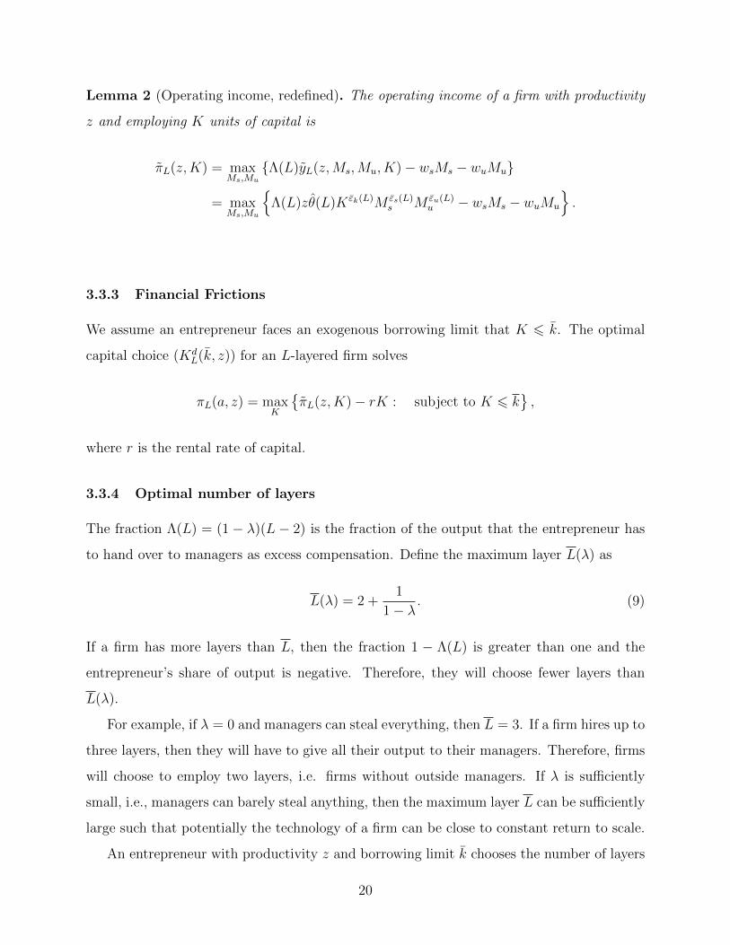
Lemma 2 (Operating income, redefined). The operating income of a firm with productivity

z and employing K units of capital is

πL(z,K) = maxMs,Mu

{Λ(L)yL(z,Ms,Mu, K)− wsMs − wuMu}

= maxMs,Mu

{Λ(L)zθ(L)K εk(L)M εs(L)

s M εu(L)u − wsMs − wuMu

}.

3.3.3 Financial Frictions

We assume an entrepreneur faces an exogenous borrowing limit that K 6 k. The optimal

capital choice (KdL(k, z)) for an L-layered firm solves

πL(a, z) = maxK

{πL(z,K)− rK : subject to K 6 k

},

where r is the rental rate of capital.

3.3.4 Optimal number of layers

The fraction Λ(L) = (1 − λ)(L − 2) is the fraction of the output that the entrepreneur has

to hand over to managers as excess compensation. Define the maximum layer L(λ) as

L(λ) = 2 +1

1− λ. (9)

If a firm has more layers than L, then the fraction 1 − Λ(L) is greater than one and the

entrepreneur’s share of output is negative. Therefore, they will choose fewer layers than

L(λ).

For example, if λ = 0 and managers can steal everything, then L = 3. If a firm hires up to

three layers, then they will have to give all their output to their managers. Therefore, firms

will choose to employ two layers, i.e. firms without outside managers. If λ is sufficiently

small, i.e., managers can barely steal anything, then the maximum layer L can be sufficiently

large such that potentially the technology of a firm can be close to constant return to scale.

An entrepreneur with productivity z and borrowing limit k chooses the number of layers

20

to maximize profit given by

π(k, z) = maxL<L(λ)

{πL(k, z)

}. (10)

Let L∗(k, z) be the solution to the above optimization problem.9

3.4 Aggregation and Equilibrium

LetG(k, z) be the joint distribution of entrepreneurial households over the exogenous borrow-

ing limit and productivity. Aggregate capital demand, skilled labor demand, and unskilled

labor demand are

Kd = Ne

∫k,z

Kd(k, z)G(dk, dz), (11)

Mds = Ne

∫k,z

Mds (k, z)G(dk, dz), (12)

Mdu = Ne

∫k,z

Mdu(k, z)G(dk, dz), (13)

where Kd(k, z), Mds (k, z), and Md

u(k, z) are the demand of capital, skilled labor, and unskilled

labor of an individual firm with borrowing limit k and productivity z whose problem is solved

previously.

We now define the stationary equilibrium as follows:

Definition 2 (Competitive Equilibrium). A competitive equilibrium for this economy con-

sists of prices r and w, optimal input and layer choices Kd(k, z), Mds (k, z), Md

u(k, z), and

L∗(k, z), optimal labor supply Ns(ws, wu) and Nu(ws, wu), that satisfy the following condi-

tions:

i) Given prices and borrowing limits, Kd(k, z), Mds (k, z), Mu(k, z), and L∗(k, z) solves

the firm’s problem.

ii) Given prices, the worker households choose the amount of skilled and unskilled labor

that are supplied to the market subject to Ns(ws, we) +Nu(ws, we) 6 Ne.

9Note that we are not able to show that there is an unique solution, though in practice there has alwaysbeen an unique solution. If there are multiple solutions, we will take the smaller one.

21

iii) The interest rate r clears the capital market: Ks = Kd, where Ks is the endowment of

capital in this economy.

iv) The wage ws and wu clear the labor market: Ns =Mds and Nu =Md

u.

3.5 Model properties

We now highlight some properties of the model relevant to our analysis.

Proposition 1. The optimal number of layers L∗(a, z) is weakly increasing in entrepreneurial

productivity (z) and borrowing limit (k).

The optimal number of layers is increasing in the firm’s productivity because firm pro-

ductivity z and and input are complements. Therefore, a more productive firm gains more

than a less productive firm from increasing the number of layers.

Lemma 3, which follows closely from proposition 1, shows that the support of the pro-

ductivity distribution conditional on the borrowing limit can be partitioned into intervals

within which all firms choose the same number of layers.

Lemma 3. There exists an increasing sequence of threshold productivities {z(L, k)} such

that for z ∈ [z(L, k), z(L+ 1, k)), the optimal number of layers L∗(z, k) is L.

Proposition 2. In the economy without financial frictions (k = +∞), capital and labor

demand are strictly increasing in the firm’s productivity z.

Proposition 3 (Declining APK without managerial friction). In an economy without fric-

tions (λ = 1 and k = +∞), the average product of capital is declining in firm productivity z

and firm size.

The average product of capital is falling with productivity because the number of layers,

and therefore the span of control, is increasing. The marginal product is, however, constant

and equals r.

22

3.5.1 Economies with Contracting Frictions with Managers (λ < 1)

The contracting friction with outside managers disproportionately affects more productive

firms. First, they are forced to reduce the number of layers in their organizational structure.

Second, if they continue to hire outside managers, they must adjust their scale downward.

Lemma 4 shows that this manifests as a higher marginal product of capital.

Lemma 4. In an economy with λ ∈ (0, 1) where some firms still hire outside managers, the

marginal product of capital is increasing in firm productivity z:

MPK(z) =r

Λ(L∗(z)).

Lemma 5 characterizes the wage premia earned by managers, as a function of the layer

they are employed in and their employer’s productivity z.

Lemma 5. The wage premium earned by an outside manager working at the lth layer at a

firm with productivity z is

b(l, z) =1− λθl

[1

Λ(L∗(z))

(W

(1− θ)

)] 1ν(L∗(z))

The wage premium is increasing in the layer the manager works at (l) and the firm’s pro-

ductivity z.

The wage premium is increasing with the manager’s layer not because higher higher-

level managers are more productive, but because there are fewer of them. Since more output

passes through each manager’s hands, they need to be compensated more to prevent stealing.

The higher productivity of the firm increases the wage premium only if the firm employs

more layers. Although a higher productivity also directly increases output, it also increases

the number of managers at each level and these effects cancel out.

4 Quantitative Analysis

We calibrate our model with perfect contract enforcement between entrepreneurs and outside

managers (λ = 1) and financial frictions to moments from US data. By doing this, we are

23

able to determine the value of parameters governing technologies and ability distribution.

We then recalibrate the parameters governing both frictions, as well as some productivity

parameters, to firm-level and household-level data of China, and study how both frictions

affect aggregate productivity.

4.1 Calibration Strategy

We first describe how we calibrate the model without managerial frictions to the U.S. data.

There are in total seven parameters of this model: four on technology, {α, θ, µ, γ}, one on

skill accumulation {κ}, and two on endowments {Ne, Nw}. In addition, we need to determine

the joint distribution of entrepreneur’s ability z and the financial frictions k.

Technology: {α, θ, µ, γ}. The capital share α is set to 0.33 following Gollin (2002). The

parameter θ determines the efficiency of supervision. We choose θ to match the moment

that 12.0% of household labor works as managers in the Integrated Public Use Microdata

Series (IPUMS) USA 2005 census data (Ruggles et al., 2017). µ and γ govern the relative

importance of skilled labor versus unskilled among workers and different layers of managerial

resources. We choose these two parameters to match the following two moments: 1) the

portion of skilled workers, which is approximated by the portion of college graduates, is

53.0% from the IPUMS-USA data; 2) the elasticity between firm size and average wage

of a firm is 0.047 (Troske, 1999). The second moment is informative as larger firms hire

on average more skilled workers in the managerial layers, and therefore the average labor

productivity can be higher even without frictions.

Skill Accumulation: {κ}. κ determines the schooling cost of a skilled worker. It deter-

mines the wage premium of skilled labor relative to unskilled labor. Since we use college

graduates to approximate skilled labor, we choose κ to match a college wage premium of

47.6% as we observed in the IPUMS-USA data.

Endowments: {Ne, Nw}. Ne and Nw determine the relative measure of entrepreneurs

versus household labor (which is the sum of measures of workers and managers, or the sum

24

of measures of skilled and unskilled labor). IPUMS-USA data set has no information on

whether an individual works as a manager. Cagetti and Nardi (2006) use the Survey of

Consumer Finances (SCF) and report that 7.55% of the population work as entrepreneurs

in the U.S. We therefore normalize Nw = 1, and choose Ne = 8.17% such that the share of

entrepreneurs is Ne/(Ne +Nw) = 8.17%/(1 + 8.17%) = 7.55%.

The Distribution of Ability and Financial Frictions {F (z, k)}. We assume that

entrepreneurial productivity z follows a log-Normal distribution with a mean of zero and

a standard deviation of σ. We discipline σ by targeting the moment that 69% of workers

are employed by firms in the top 10% of the size distribution. Although the log-normal

distribution typically cannot match the employment shares in the tail of size distribution,

we are able to do so because these large firms increase their span of control by hiring outside

managers.

For the financial frictions, we follow Bento and Restuccia (2017) and assume that the

exogenous borrowing limit takes the following functional form:

log ki = β0 + β1 log zi + εi, (14)

where β1 determines the correlation between the distortion and ability, while εi is a random

variable following normal distribution with standard deviation of σε. These two parame-

ters govern the correlation between sales-to-asset ratio and firm size, and the variation of

sales-to-asset ratio among firms of the same size. Crouzet and Mehrotra (2018) argue that

the US Census Bureau’s Quarterly Financial Report (QFR) provide a representative sam-

ple of the population of U.S. manufacturing firms, while the sample of Compustat is not

representative. Therefore, we take two moments from Crouzet and Mehrotra (2018): 1) the

quarterly sales-to-asset ratio is 0.60 among firms within the size distribution from zero to

90th percentile, while it is 0.39 among firms within the size distribution from 90th to 99th

percentile, meaning that the ratio is around 54% higher for smaller firms; 2) among firms

within the size distribution from zero to 99th percentile, the average leverage ratio is 0.35,

while those firms with leverages in the upper quartile (> p75) has an average leverage ratio

of 0.47, the ratio of which provides the dispersion of leverage among firms. Note that in

25

our model, we do not have the separation of assets and debts, but we use the dispersion of

the the leverage ratio to approximate that of the capital-to-sales ratio, as in our model, the

dispersion only arises from financial frictions.

Re-Calibration to Chinese Data: {Ne, Nw, κ, λ, F (z, k)}. Previously we calibrate our

model to the U.S. data to pin down the parameters governing technology and ability dis-

tribution. Our goal is to study how the frictions can explain the observed pattern in the

Chinese data, so we further re-calibrate some parameters to reflect the salient features in the

Chinese data. First we choose Nw = 1 and Ne = 0.042 such that 3.99% of population works

as entrepreneurs in the 2005 Chinese Household Census. We choose κ such that the wage of

skilled labor working as production workers is around 47.5% higher than that of unskilled

labor working as production workers, after controlling for observables such as age, gender,

health status, and marriage status. We choose λ to match the moment that, the wage of

skilled labor working as managers is around 49.3% higher than that of skilled labor working

as workers, after the same set of controls.

We re-calibrate β1 and σε in Equation (14) to match two moments from 2004 Chinese

Manufacturing Enterprise Census: 1) the elasticity between capital-to-output ratio and firm

size (measured by capital) is 0.49, after controlling for firm age, industry, region, and own-

ership; 2) the standard deviation of the residual of log capital-to-output ratio is 1.025, after

controlling for firm size, firm age, industry, region, and ownership. Note that we avoid using

labor to measure firm size as we described before that there is selection among small firms

and the sample is not representative.

4.2 Contracting frictions and aggregate productivity

In our first quantitative exercise, we investigate the effect of increasing the fraction outside

managers can steal (i.e. reducing λ), while maintaining the assumption of no financial

frictions (i.e. φ = 1). Figure 10 presents the impact on aggregate productivity.

26

Fraction managers can steal (λ)0.5 0.55 0.6 0.65 0.7 0.75 0.8 0.85 0.9 0.95 1

TF

P

0.75

0.8

0.85

0.9

0.95

1

Figure 10: TFP and contracting frictions with managers

In figure 10, we normalize TFP by the level in the frictionless economy.10 Aggregate

productivity falls monotonically to 76% as the contracting friction with managers worsen.

When the friction gets sufficiently worse, entrepreneurs stop hiring outside managers.

Figure 11 shows how the fraction of workers employed as outside managers changes as the

contracting friction worsens. Entrepreneurs respond to the contracting frictions by hiring

fewer outside managers.

10TFP equals 1 when λ = 1.

27

Contracting friction with outside manager (λ)0.6 0.65 0.7 0.75 0.8 0.85 0.9 0.95 1

Fra

ctio

n o

f w

ork

ers

em

plo

yed

as

ou

tsid

e m

ana

ge

rs

0

0.05

0.1

0.15

0.2

0.25

0.3

0.35

0.4

Figure 11: Fraction employed as outside managers

We next study the impact of financial frictions (12), by varying the fraction φ lenders can

recoup from defaulting entrepreneurs. We do this both for an economy without contracting

frictions between entrepreneurs and managers (blue line), and severe contracting frictions

between entrepreneurs and managers (red line). We again normalize productivity by that

obtained in the frictionless economy.

Productivity falls monotonically as financial frictions worsen, but the total fall is about

5%. The productivity drop is at the lower end of those reported in the literature because

we have shut down occupational choice. Distorted selection is often the main driver of

productivity losses from financial frictions (as in Buera et al. (2011)).11

Figure 12 suggests that there is little interaction between the two frictions. It is interesting

to note that in the economy with severe managerial frictions, the impact of financial frictions

is smaller. This is because managerial frictions, by effectively compressing the underlying

distribution of firm productivity, reduce the scope for financial frictions to further lower

aggregate productivity.

11We abstract from occupational choice both for technical reasons (see discussion in 3) and because ourobjective is mainly to asset factor misallocation across operating firms.

28

Financial friction (φ)0 0.1 0.2 0.3 0.4 0.5 0.6 0.7 0.8 0.9 1

TF

P

0.7

0.75

0.8

0.85

0.9

0.95

1

No managerial frictions (λ = 1)Managerial frictions

Figure 12: TFP and financial frictions

4.3 Cross-sectional properties

In figure 13, we present some preliminary analysis of how the managerial contracting friction

affects delegation decisions and wedges. In figure 13, we plot the number of layers against

firm productivity. Consistent with our analytical results, the number of layers is (weakly) in-

creasing in firm productivity. As we tighten contracting frictions, the number of managerial

layers decline. As low-productivity firms do not employ outside managers in the absence of

the friction, they are not affected at all as the friction worsens. However, highly-productive

firms do want to employ outside managers and therefore disproportionately affected by wors-

ening managerial frictions.

29

Productivity (z)

Nu

mb

er

of

ma

na

ge

ria

l la

yers

1

2

3

4

5

6

7

λ = 1λ = 0.9λ = 0.8

Figure 13: Number of managerial layers

Next we illustrate how our model is able to generate larger distortions for larger firms.

We consider two economies: One economy has managerial frictions and the other does not.12.

In the first economy, all firms equate marginal product of capital to the rental rate. In the

economy with managerial frictions, large firm still find it optimal to hire outside managers.

However, one way they reduce the incentive to steal is by reducing their scale of operation

which raises the marginal product of capital above the rental rate.

12Both do not have financial frictions

30

Capital (quintiles)

0 2 4 6 8 10 12 14 16 18 20

MP

K -

R

-0.04

-0.02

0

0.02

0.04

0.06

0.08

0.1

0.12

No managerial frictions (λ = 1)Managerial frictions

Figure 14: Marginal product of capital and firm size

5 Conclusion

In this paper, propose that weak contract enforcement between firms and outside managers

is an important source of factor misallocation and productivity losses. We document that

marginal products of capital and labor are increasing in firm size and that managers in de-

veloping countries receive higher compensation. We develop a model where productive firms

hire outside managers to increase their span of control. These firms respond to contracting

frictions with managers by paying efficiency wages (which result in output wedges), and

by reducing their scale of operation. Our quantitative exercises show how this friction can

lead to much larger productivity losses than financial frictions, and is consistent with the

relationship between firm size and marginal products we document in the data.

31

References

Acemoglu, D., Johnson, S., and Robinson, J. A. (2005). Institutions as a fundamental cause

of long-run growth. Handbook of Economic Growth, 1(A):385–472.

Akcigit, U., Alp, H., and Peters, M. (2017). Lack of Selection and Limits to Delegation:

Firm Dynamics in Developing Countries. Working Paper.

Alchian, A. A. and Demsetz, H. (1973). The Property Right Paradigm. Journal of Economic

History, 33(1):16–27.

Bento, P. and Restuccia, D. (2017). Misallocation, Establishment Size, and Productivity.

American Economic Journal: Macroeconomics, 9(3):267–303.

Bloom, N. and Reenen, J. V. (2007). Measuring and Explaining Management Practices

Across Firms and Countries. The Quarterly Journal of Economics, 122(4):1351–1408.

Bloom, N. and Reenen, J. V. (2010). Why Do Management Practices Differ across Firms

and Countries? Journal of Economic Perspectives, 24(1):203–224.

Brandt, L. and Zhu, X. (2010). Accounting for China’s Growth. Working Paper.

Buera, F. J., Kaboski, J. P., and Shin, Y. (2011). Finance and Development: A Tale of Two

Sectors. American Economic Review, 101(5):1964–2002.

Cagetti, M. and Nardi, M. D. (2006). Entrepreneurship, frictions and wealth. Journal of

Political Economy, 114(5):835–870.

Caselli, F. (2005). Accounting for cross-country income differences. Handbook of Economic

Growth, 1:679 – 741.

Crouzet, N. and Mehrotra, N. R. (2018). Small and Large Firms Over the Business Cycle.

Working Paper.

Garicano, L. and Rossi-Hansberg, E. (2006). Organization and Inequality in a Knowledge

Economy. Quarterly Journal of Economics, 121(4):1383–1435.

Gollin, D. (2002). Getting Income Shares Right. Journal of Political Economy, 110(2):458–

474.

Grobovsek, J. (2017). Managerial Delegation and Aggregate Productivity. Working Paper.

32

Haltiwanger, J., Jarmin, R. S., and Miranda, J. (2013). Who Creates Jobs? Small versus

Large versus Young. Review of Economics and Statistics, 95(2):347–361.

Hsieh, C.-T. and Klenow, P. J. (2009). Misallocation and Manufacturing TFP in China and

India. Quarterly Journal of Economics, 124(4):1403–1448.

Hsieh, C.-T. and Klenow, P. J. (2014). The Life Cycle of Plants in India and Mexico.

Quarterly Journal of Economics, 129(3):1035–1084.

Hsieh, C.-T. and Olken, B. A. (2014). The Missing “Missing Middle”. Journal of Economic

Perspectives, 28(3):89–108.

Lucas, Jr., R. E. (1978). On the size distribution of business firms. Bell Journal of Economics,

9(2):508–523.

Moll, B. (2014). Productivity Losses from Financial Frictions: Can Self-Financing Undo

Capital Misallocation? American Economic Review, 104(10):3186–3221.

Restuccia, D. and Rogerson, R. (2008). Policy distortions and aggregate productivity with

heterogeneous establishments. Review of Economic Dynamics, 11(4):707–720.

Roys, N. and Seshadri, A. (2014). Economic Development and the Organization of Produc-

tion. Working Paper.

Ruggles, S., Genadek, K., Goeken, R., Grover, J., and Sobek, M. (2017). Integrated Public

Use Microdata Series: Version 7.0 [Dataset]. Minneapolis: University of Minnesota.

Troske, K. (1999). Evidence on the employer size-wage premium from worker-establishment

matched data. Review of Economics and Statistics, 81(1):15–26.

33