Continuous Optimisation, Chpt 2: Unconstrained...

Introduction Optimality Conditions Solution methods

Continuous Optimisation, Chpt 2:Unconstrained Optimisation

Peter J.C. Dickinson

DMMP, University of Twente

[email protected]

http://dickinson.website/Teaching/2017CO.html

version: 28/09/17

Monday 25th September 2017

Peter J.C. Dickinson http://dickinson.website CO17, Chpt 2: Unconstrained Optimisation 1/21

http://dickinson.website/Teaching/2017CO.html


Literature: KRT 2.1 and 4.



Table of Contents

1 Introduction

2 Optimality ConditionsGeometry of minimisationDescent directionsNecessary/sufficient conditionsConvex functions

3 Solution methods



Geometry of minimisation

Theorem 2.1 (Geometry of minimisation)

Consider f : Rn → R, f ∈ C1 and a point y ∈ F with ∇f (y) 6= 0.In a neighbourhood of y the set Dy = {x ∈ F : f (x) = f (y)} is aC1-manifold of dimension n − 1, and at y we have ∇f (y) ⊥ Dy.



Example

http://ggbm.at/e3vayUbW

f (x1, x2) = 1100(x21 + x22 )((x1 − 5)2 + (x2 − 1)2)((x1 − 2)2 + (x2 − 3)2 + 1)

Three strict local minima, two of which are global minima.Peter J.C. Dickinson http://dickinson.website CO17, Chpt 2: Unconstrained Optimisation 5/21

http://ggbm.at/e3vayUbW


Descent directions

Definition 2.2

For f : Rn → R and x ∈ Rn, we call h ∈ Rn a strict descentdirection of f at x if ∃ε > 0 s. t. f (x + εh) < f (x) for all ε ∈ (0, ε].

Fill in the quiz at www.shakeq.com, login code utwente118.

Lemma 2.3

For x ∈ Rn and f : Rn → R consider the following statements:

1 x is a global minimiser of f ;

2 x is a local minimiser of f ;

3 There are no strict descent directions of f at x.

We have (1)⇒ (2)⇒ (3). If f is convex then (1)⇔ (2)⇔ (3)


www.shakeq.com


Exercises

Ex. 2.1 Prove Lemma 2.3.

Ex. 2.2 Consider f (x1, x2) = (x21 − 2x2)(x21 − x2). Show that:

(a) the origin 0 is not a local minimiser of f ;

(b) all h ∈ Rn \ {0} are strict ascent directions of f at 0, i.e. forall h ∈ Rn \ {0}, ∃ε > 0 s. t. f (εh) > f (0) for all ε ∈ (0, ε].

N.B. Therefore, in this nonconvex example, statement (3) ofLemma 2.3 holds, but not statement (1).We thus see that for nonconvex problems even if every directionwill lead to an increase, we may still not have a local minimum.



Necessary/sufficient conditions

Theorem 2.4

For f ∈ C2 and ‖h‖ small:

f (x + h) = f (x) +∇f (x)Th + 12h

T∇2f (x)h + o(‖h‖2).

Corollary 2.5 (Necessary condition)

Consider f : Rn → R, f ∈ C1 (resp. f ∈ C2). If x ∈ Rn is a localminimiser then ∇f (x) = 0 (resp. ∇2f (x) � O).

N.B. Not sufficient, e.g. f (x) = x3, − x4, − exp(−x−2).

Corollary 2.6 (Sufficient condition)

Consider f : Rn → R, f ∈ C2. If x ∈ Rn has ∇f (x) = 0 and∇2f (x) � O then x is a strict local minimiser of f .

N.B. Not Necessary, e.g. f (x) = x4, exp(−x−2)Peter J.C. Dickinson http://dickinson.website CO17, Chpt 2: Unconstrained Optimisation 8/21


Convex functions

Corollary 2.7 (from Theorem 1.21 and Corollary 2.5)

For a convex function f : Rn → R, f ∈ C1 and x0 ∈ Rn thefollowing are equivalent:

1 x0 is a global minimum,

2 x0 is a local minimum,

3 ∇f (x0) = 0.

Lemma 2.8

The set of global minimisers of a convex function is a convex set.



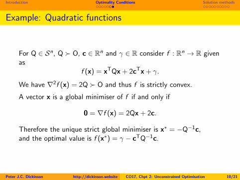
Example: Quadratic functions

For Q ∈ Sn, Q � O, c ∈ Rn and γ ∈ R consider f : Rn → R givenas

f (x) = xTQx + 2cTx + γ.

We have ∇2f (x) = 2Q � O and thus f is strictly convex.

A vector x is a global minimiser of f if and only if

0 = ∇f (x) = 2Qx + 2c.

Therefore the unique strict global minimiser is x∗ = −Q−1c,and the optimal value is f (x∗) = γ − cTQ−1c.



Table of Contents

1 Introduction

2 Optimality Conditions

3 Solution methodsBasic IdeaDescent directionsChoosing dNewton’s method(Dis)advantagesOther methodsStopping Criteria



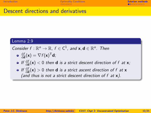
Descent directions and derivatives

Lemma 2.9

Consider f : Rn → R, f ∈ C1, and x,d ∈ Rn. Thendfdd(x) = ∇f (x)Td;

If dfdd(x) < 0 then d is a strict descent direction of f at x;

If dfdd(x) > 0 then d is a strict ascent direction of f at x

(and thus is not a strict descent direction of f at x).



Basic idea

Basic idea for minimising a function f : Rn → (R ∪ {∞}), f ∈ C1

over Rn:

1 Start at a point x0 ∈ Rn. (k = 0)

2 Find a search direction dk ∈ Rn such that dfddk

(xk) < 0.

3 If no such direction exists then STOP.

4 Line search: Find λk = arg minλ{f (xk + λdk) : λ ∈ R}(or just f (xk + λkdk) < f (xk)). [See KRT, 4.3]

5 Let xk+1 = xk + λkdk and k ← k + 1.

6 If stopping criteria satisfied then STOP, else go to step 2.



Choosing d: First order

Lemma 2.10

For f ∈ C1(Rn,R) and x,d ∈ Rn we have ∂f∂d(x) = ∇f (x)Td and

f (x + λd) = f (x) + λ∇f (x)Td + o(λ).

Lemma 2.11

For f ∈ C1(Rn,R) and x ∈ Rn s.t. ∇f (x) 6= 0 we have

arg mind{∇f (x)Td : ‖d‖2 = 1} = − ∇f (x)

‖∇f (x)‖2 .

d = − ∇f (x)‖∇f (x)‖2 is the direction of steepest descent.

Ex. 2.3 For xk+1,dk as given on the previous slide withλk = arg minλ{f (xk + λdk) : λ ∈ R}, show that dTk∇f (xk+1) = 0.



Example: Quadratic optimisation

Ex. 2.4 Do exercise 4.15 from KRT.

https://ggbm.at/TYBdQDeB

The convergence to the optimal can be quite slow.

This is a problem in general for minimising a function f ∈ C2, as ifat a minimiser x∗ we have ∇2f (x∗) � O, and then forA = 1

2∇2f (x∗) � O, c = −Ax∗, γ = f (x∗) + x∗TAx∗ we have

f (x) ≈ f (x∗) + (x− x∗)TA(x− x∗) = xTAx + 2cTx + γ for x ≈ x∗.


https://ggbm.at/TYBdQDeB


Newton’s methodLemma 2.12

For f ∈ C2(Rn,R) and x,d ∈ Rn we have

f (x + d) = f (x) +∇f (x)Td + 12d

T∇2f (x)d + o(‖d‖2).

Letting Q = 12∇

2f (xk), c = 12∇f (xk) and γ = f (xk) we have

f (xk + d) ≈ dTQd + 2cTd + γ.If Q � O then, as a function of d, we have that the right-hand sideis minimised at d = −Q−1c = −

(∇2f (xk)

)−1∇f (xk).Referred to as Newton’s direction, and works well as a searchdirection (often with λk = 1, xk+1 = xk −

(∇2f (xk)

)−1∇f (xk),e.g. https://ggbm.at/qMX5uqcF ).Finds minimum in one step for quadratic functions.

Ex. 2.5 Show that if A � O, ∇f (xk) 6= 0 and dk = −A∇f (xk)then dTk∇f (xk) < 0, and thus dk is a descent direction.Which choices of A give the steepest descent and the Newton’sdirection respectively?


https://ggbm.at/qMX5uqcF


(Dis)advantages

(+) Newton’s method normally converges quicker (in terms ofnumber of steps).

(+) With Newton’s method it is normally sufficient to consider astep length of one, so no line search necessary.

(–) For steepest descent method we need only compute thegradient vector ∇f (xk), whereas for Newton’s method we

need to also compute the Hessian and(∇2f (xk)

)−1∇f (xk).

(–) With Newton’s method, we require that the Hessian matrix ispositive definite.



Exercise

Ex. 2.6 Consider the (convex) function f : R2 → R given by

f (x) = exp(x21 + 2x22

).

(N.B. The global minimiser is at x∗ = 0.)

For the starting point x0 =(0.6 0.6

)T, perform the first 7

iterations (i.e. find x1, . . . , x7) for:

1 the steepest descent method;

2 Newton’s method without line search;

3 Newton’s method with line search.



Other methods

There are also plenty of other methods, e.g.:

Conjugate gradient method;

Quasi-Newton method;

Stochastic gradient descent;

Simulated annealing.



Stopping Criteria

Upper bound given by f (xk) ∈ R, i.e. infx{f (x) : x ∈ Rn} ≤ f (xk).

Could stop after certain number of iterations.

If also have lower bounds Lk ∈ R (e.g. duality, see later in course),can pick parameter ε > 0 and stop when

f (xk)− Lk1 + |f (xk)|

≤ ε,

i.e. relative difference between upper and lower bounds small.

If no (good) lower bounds, can pick parameter ε > 0 and stopwhen

f (xk)− f (xk+1)

1 + |f (xk)|≤ ε,

i.e. relative improvement small.Peter J.C. Dickinson http://dickinson.website CO17, Chpt 2: Unconstrained Optimisation 20/21


Ex. 2.7 Assuming

xk+1 = xk + dk , and

f (xk+1) ≈ f (xk) + dTk∇f (xk) + 12d

Tk∇2f (xk)dk

when considering Newton’s method, what is

f (xk)− f (xk+1)

approximately equal to, as a function of xk?


Continuous Optimisation, Chpt 2: Unconstrained...

Documents

Transcript of Continuous Optimisation, Chpt 2: Unconstrained...