Contents lists available at ScienceDirect ...nrb250/papers/BFG2011.pdf · Contents lists available...
30
Journal of Combinatorial Theory, Series A 118 (2011) 2261–2290 Contents lists available at ScienceDirect Journal of Combinatorial Theory, Series A www.elsevier.com/locate/jcta The enumeration of prudent polygons by area and its unusual asymptotics Nicholas R. Beaton a , Philippe Flajolet b , Anthony J. Guttmann a a ARC Centre of Excellence for Mathematics and Statistics of Complex Systems, Department of Mathematics and Statistics, The University of Melbourne, Victoria 3010, Australia b Algorithms Project, INRIA–Rocquencourt, 78153 Le Chesnay, France article info abstract Article history: Received 6 December 2010 Available online xxxx Keywords: Asymptotics Prudent polygons Area enumeration Mellin transforms q-Series Prudent walks are special self-avoiding walks that never take a step towards an already occupied site, and k-sided prudent walks (with k = 1, 2, 3, 4) are, in essence, only allowed to grow along k direc- tions. Prudent polygons are prudent walks that return to a point adjacent to their starting point. Prudent walks and polygons have recently been enumerated by length and perimeter by Bousquet- Mélou and Schwerdtfeger. We consider the enumeration of pru- dent polygons by area. For the 3-sided variety, we find that the generating function is expressed in terms of a q-hypergeometric function, with an accumulation of poles towards the dominant sin- gularity. This expression reveals an unusual asymptotic structure of the number of polygons of area n, where the critical exponent is the transcendental number log 2 3 and the amplitude involves tiny oscillations. Based on numerical data, we also expect similar phenomena to occur for 4-sided polygons. The asymptotic method- ology involves an original combination of Mellin transform tech- niques and singularity analysis, which is of potential interest in a number of other asymptotic enumeration problems. Crown Copyright © 2011 Published by Elsevier Inc. All rights reserved. 1. Introduction The problem of enumerating self-avoiding walks (SAWs) and polygons (SAPs) on a lattice is a famous one, whose complete solution has thus far remained most elusive. For the square lattice, it is conjec- tured that the number SAW n of walks of length n and the number SAP n of polygons of perimeter n each satisfy an asymptotic formula of the general form E-mail address: [email protected] (A.J. Guttmann). 0097-3165/$ – see front matter Crown Copyright © 2011 Published by Elsevier Inc. All rights reserved. doi:10.1016/j.jcta.2011.05.004
Transcript of Contents lists available at ScienceDirect ...nrb250/papers/BFG2011.pdf · Contents lists available...

Journal of Combinatorial Theory, Series A 118 (2011) 2261–2290
Contents lists available at ScienceDirect
Journal of Combinatorial Theory,Series A
www.elsevier.com/locate/jcta
The enumeration of prudent polygons by areaand its unusual asymptotics
Nicholas R. Beaton a, Philippe Flajolet b, Anthony J. Guttmann a
a ARC Centre of Excellence for Mathematics and Statistics of Complex Systems, Department of Mathematics and Statistics,The University of Melbourne, Victoria 3010, Australiab Algorithms Project, INRIA–Rocquencourt, 78153 Le Chesnay, France
a r t i c l e i n f o a b s t r a c t
Article history:Received 6 December 2010Available online xxxx
Keywords:AsymptoticsPrudent polygonsArea enumerationMellin transformsq-Series
Prudent walks are special self-avoiding walks that never take a steptowards an already occupied site, and k-sided prudent walks (withk = 1,2,3,4) are, in essence, only allowed to grow along k direc-tions. Prudent polygons are prudent walks that return to a pointadjacent to their starting point. Prudent walks and polygons haverecently been enumerated by length and perimeter by Bousquet-Mélou and Schwerdtfeger. We consider the enumeration of pru-dent polygons by area. For the 3-sided variety, we find that thegenerating function is expressed in terms of a q-hypergeometricfunction, with an accumulation of poles towards the dominant sin-gularity. This expression reveals an unusual asymptotic structureof the number of polygons of area n, where the critical exponentis the transcendental number log2 3 and the amplitude involvestiny oscillations. Based on numerical data, we also expect similarphenomena to occur for 4-sided polygons. The asymptotic method-ology involves an original combination of Mellin transform tech-niques and singularity analysis, which is of potential interest in anumber of other asymptotic enumeration problems.
Crown Copyright © 2011 Published by Elsevier Inc.All rights reserved.
1. Introduction
The problem of enumerating self-avoiding walks (SAWs) and polygons (SAPs) on a lattice is a famousone, whose complete solution has thus far remained most elusive. For the square lattice, it is conjec-tured that the number SAWn of walks of length n and the number SAPn of polygons of perimeter neach satisfy an asymptotic formula of the general form
E-mail address: [email protected] (A.J. Guttmann).
0097-3165/$ – see front matter Crown Copyright © 2011 Published by Elsevier Inc. All rights reserved.doi:10.1016/j.jcta.2011.05.004
2262 N.R. Beaton et al. / Journal of Combinatorial Theory, Series A 118 (2011) 2261–2290
C · μn · nβ, (1)
where C,μ ∈ R>0 and β ∈ R. (In the case of polygons, it is understood that n must be restricted toeven values.) The number μ is the “growth constant” and the number β is often referred to as the“critical exponent”. More precisely, the following expansions are conjectured,
SAWn ∼n→∞ C1 · μn · n11/32, SAPn ∼
n→∞ C2 · μn · n−5/2, (2)
for some C1, C2 > 0.For the square lattice, numerical methods based on acceleration of convergence and differential
approximants suggest the value μ = 2.6381585303 . . . . This estimate is indistinguishable from the so-lution of the biquadratic equation 13μ4 −7μ2 −581 = 0, which we consider to be a useful mnemonic.This was observed by Conway, Enting and Guttmann [6] in 1993, and verified to 11 significant dig-its by Jensen and Guttmann [23] in 2000, based on extensive numerical analysis of the sequence(SAP2n) up to n = 45. (Remarkably enough, for the honeycomb lattice, it had long been conjectured
that the growth constant of walks is the biquadratic number√
2 + √2, a fact rigorously established
only recently by Duminil-Copin and Smirnov [13].)As regards critical exponents, the conjectured value β = 11
32 for walks is supported by results ofLawler, Schramm, and Werner that relate the self-avoiding walk to the “stochastic Loewner Evolution”(SLE) process of index 8/3; see, for instance, the account in Werner’s inspiring lecture notes [37].For (unrooted) polygons, the value β = − 5
2 was suggested by numerical analysis of the exact countingsequence, with an agreement to the seventh decimal place [23]. It is also supported by the observationthat many simplified, exactly solvable, (naturally rooted) models of self-avoiding polygons appear toexhibit an n−3/2 universal behavior — for these aspects, we refer to the survey by Bousquet-Mélouand Brak [4], as well as the books [15,20,32].
Regarding lattice polygons, which are closed walks, there is also considerable interest in enumer-ation according to area, rather than perimeter. There are at least two reasons for this. Enumeratingpolygons by both perimeter and area provides a very natural and powerful model of vesicles, withconsiderable biological interest [32]. Secondly, it is closely related to the classical unsolved problemof enumerating polyominoes (also known as animals), according to the number of cells they contain.Polygons are a proper subset of polyominoes, so any results obtained on polygons enumerated by areamay illuminate the polyomino enumeration problem.
Conjecturally [24], the number an (respectively, bn) of polygons (respectively, polyominoes) com-prised of n cells satisfies asymptotic estimates of the form
an ∼n→∞ C3 · (3.9709 . . .)n · n−1, bn ∼
n→∞ C4 · (4.0625 . . .)n · n−1,
for some C3, C4 ∈ R>0; these asymptotic estimates are still of the form (1), with the critical exponentβ = −1. Interestingly enough, the critical exponent β = 0, corresponding to a simple pole of theassociated generating function, is otherwise known to arise in several simplified models, such ascolumn-convex, convex, and directed polyominoes [2,4,20].
As the foregoing discussion suggests, there is considerable interest in solving, exactly, probabilis-tically, or asymptotically, restricted models of self-avoiding walks and polygons. Beyond serving todevelop informed conjectures regarding more complex models, this is relevant to areas such as sta-tistical physics and the statistical mechanics of polymers [32]. For combinatorialists, we may observethat consideration of such models has served as a powerful incentive to develop new counting meth-ods based on generating functions [4,7,20,36], including transfer matrix methods and what is knownas the “kernel method”.
The present article focuses on a special type of self-avoiding polygon, the 3-sided prudent polygon(to be defined shortly — see Definition 1 in Section 2), when these are enumerated according to area.Roughly, a walk is prudent if it never takes a step towards an already occupied site and it is 2-, 3-,4-sided if it has, respectively, 2, 3, or 4 allowed directions of growth; a prudent polygon is a prudentwalk that is almost closed. For area n, we will obtain a precise asymptotic formula (Theorem 2 below),
PAn ∼ C(n) · 2n · ng, (3)

N.R. Beaton et al. / Journal of Combinatorial Theory, Series A 118 (2011) 2261–2290 2263
one that has several distinguishing features: (i) the critical exponent is the transcendental numberg = log2 3, in sharp contrast with previously known examples where it is invariably a “small” rationalnumber; (ii) the multiplier C is no longer a constant, but a bounded quantity that oscillates around thevalue 0.10838 . . . and does so with a minute amplitude of 10−9. The oscillations cannot be revealedby any standard numerical analysis of the counting sequence PAn , but such a phenomenon may wellbe present in other models, and, if so, it could change our whole view of the asymptotic behavior ofsuch models.
Plan and results of the paper. Prudent walks are defined in Section 2, where we also introduce the2-sided, 3-sided, and 4-sided varieties. The enumeration of 2- and 3-sided walks and polygons byperimeter is the subject of insightful papers by Bousquet-Mélou [3] and Schwerdtfeger [33] who ob-tained both exact generating function expressions and precise asymptotic results. In Sections 2.2–2.4,we provide the algebraic derivation of the corresponding area results: the enumeration of 2- and3-sided prudent polygons according to area is treated there; see Theorem 1 for our first main result.For completeness, we also derive a functional equation for the generating function of 4-sided prudentpolygons (according to area), which parallels an incremental construction of [3, §6.5] — this functionalequation suffices to determine the counting sequence in polynomial time. Section 3, dedicated to theasymptotic analysis of the number of 3-sided prudent polygons, constitutes what we feel to be themain contribution of the paper. We start from a q-hypergeometric representation of the generatingfunction of interest, PA(z), and proceed to analyze its singular structure: it is found that PA(z) haspoles at a sequence of points that accumulate geometrically fast to 1
2 ; then, the Mellin transformtechnology [17] provides access to the asymptotic behavior of PA(z), as z → 1
2 in extended regionsof the complex plane. Singularity analysis [20, Chapters VI–VII] finally enables us to determine theasymptotic form of the coefficients PAn (see Theorem 2) and even derive a complete asymptotic ex-pansion (Theorem 3). As already mentioned, the non-standard character of the asymptotic phenomenafound is a distinctive feature. Section 4 concludes the paper with brief remarks relating to asymptoticmethodology. In particular, experiments suggest that similar asymptotic phenomena are likely to beencountered in the enumeration of 4-sided prudent polygons.
A preliminary announcement of the results of the present paper is the object of the communica-tion [1].
2. Prudent walks and polygons
One interesting sub-class of self-avoiding walks (SAWs) for which a number of exact solutions havebeen recently found are prudent walks. Introduced by Préa [30], these are SAWs which never take astep towards an already occupied node. Exact solutions of prudent walks on a 2-dimensional squarelattice were later studied by Duchi [11] and Bousquet-Mélou [3], who were able to enumerate certainsub-classes. The enumeration of the corresponding class of polygons is due to Schwerdtfeger [33].In this section, we first recall the definition of prudent walks and polygons, then summarize theknown results of [3,33] relative to their enumeration by length or perimeter; see Section 2.1, where2-, 3-, and 4-sided prudent walks are introduced. We then examine the enumeration of polygonsaccording to area, in each of the three non-trivial cases. The case of 2-sided polygons is easy enough(Section 2.2). The main result of this section is Theorem 1 of Section 2.3, which provides an explicitgenerating function for 3-sided polygons — it is on this expression that our subsequent asymptotictreatment is entirely based. In the case of 4-sided (i.e., “general”) polygons, we derive in Section 2.4 asystem of functional equations that determines the generating function and amounts to a polynomial-time algorithm for the generation of the counting sequence.
2.1. Main definitions and results
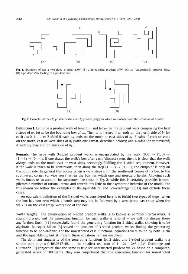
We use the same classification scheme as the authors of [3,33]. By definition, the endpoint of everyprudent walk always lies on the boundary of the smallest lattice rectangle which contains the entirewalk, referred to here as the bounding box or just box. This property leads to a natural classificationof prudent walks (see Fig. 1).
2264 N.R. Beaton et al. / Journal of Combinatorial Theory, Series A 118 (2011) 2261–2290
Fig. 1. Examples of (A) a two-sided prudent SAW; (B) a three-sided prudent SAW; (C) an (unrestricted) prudent SAW;(D) a prudent SAW leading to a prudent SAP.
Fig. 2. Examples of the (A) prudent walks and (B) prudent polygons which we exclude from the definition of 3-sided.
Definition 1. Let ω be a prudent walk of length n, and let ωi be the prudent walk comprising the firsti steps of ω. Let bi be the bounding box of ωi . Then ω is 1-sided if ωi ends on the north side of bi foreach i = 0,1, . . . ,n; 2-sided if each ωi ends on the north or east sides of bi ; 3-sided if each ωi endson the north, east or west sides of bi (with one caveat, described below); and 4-sided (or unrestricted)if each ωi may end on any side of bi .
Remark. The issue with 3-sided prudent walks is encapsulated by the walk (0,0) → (1,0) →(1,−1) → (0,−1). If one draws the walk’s box after each (discrete) step, then it is clear that the walkalways ends on the north, east or west sides, seemingly fulfilling the 3-sided requirement. However,if the walk is taken to be continuous, then along the step (1,−1) → (0,−1), the endpoint is only onthe south side. In general this occurs when a walk steps from the south-east corner of its box to thesouth-west corner (or vice versa) when the box has width one and non-zero height. Allowing suchwalks forces us to account for structures like those in Fig. 2; while this is certainly possible, it com-plicates a number of rational terms and contributes little to the asymptotic behavior of the model. Forthis reason we follow the examples of Bousquet-Mélou and Schwerdtfeger [3,33] and exclude thesecases.
An equivalent definition of the 3-sided walks considered here is to forbid two types of steps: whenthe box has non-zero width, a south step may not be followed by a west (resp. east) step when thewalk is on the east (resp. west) side of the box.
Walks (length). The enumeration of 1-sided prudent walks (also known as partially directed walks) isstraightforward, and the generating function for such walks is rational — we will not discuss theseany further. Duchi [11] successfully found the generating function for 2-sided walks, showing it to bealgebraic. Bousquet-Mélou [3] solved the problem of 3-sided prudent walks, finding the generatingfunction to be non-D-finite. For the unrestricted case, functional equations were found by both Duchiand Bousquet-Mélou, but at present these equations remain unsolved.
The dominant singularity of the generating functions for 2-sided and 3-sided prudent walks is asimple pole at ρ = 0.4030317168 . . . , the smallest real root of 1 − 2x − 2x2 + 2x3. Dethridge andGuttmann [9] conjecture that the same is true for unrestricted prudent walks, based on a computer-generated series of 100 terms. They also conjectured that the generating function for unrestricted

N.R. Beaton et al. / Journal of Combinatorial Theory, Series A 118 (2011) 2261–2290 2265
prudent walks is non-holonomic1 (non-D-finite). Here is a summary of known results, with the esti-mates tagged with a question mark being conjectural ones:
Prudent walks Generating function Asymptotic number References
2-sided algebraic κ2 · ρ−n, ρ−1 � 2.481 Duchi [11], Bousquet-Mélou [3]3-sided non-holonomic κ3 · ρ−n, ρ−1 � 2.481 Bousquet-Mélou [3]4-sided functional equation κ4 · ρ−n, ρ−1 � 2.481 (?) Dethridge and Guttmann [9].
(4)
The values of the multipliers, after [9], are κ2 = 2.51 . . . , κ3 = 6.33 . . . and (estimated) κ4 ≈ 16.12.
Prudent polygons (perimeter). Self-avoiding polygons (SAPs) are self-avoiding walks which end at anode adjacent to their starting point (excluding walks of a single step). If the walk has length n − 1then the polygon is said to have perimeter n.
Definition 2. A prudent self-avoiding polygon (prudent polygon) is a SAP for which the underlyingSAW is prudent. In the same way, a prudent polygon is 1-sided (resp. 2-sided, etc.) if its underlyingprudent walk is 1-sided (resp. 2-sided, etc.).
A 1-sided prudent polygon starting at (0,0) must end at (0,1), thus consisting only of a singlerow of cells and having a rational generating function. The enumeration of 2- and 3-sided prudentpolygons by perimeter has been addressed by Schwerdtfeger [33]. The non-trivial 2-sided prudentpolygons are essentially inverted bargraphs [31], and so the 2-sided case has an algebraic generatingfunction. Schwerdtfeger finds the 3-sided prudent polygons to have a non-D-finite generating function.
If P P (k)(z) = ∑n�0 p(k)
n zn is defined to be the half-perimeter generating function for k-sided
prudent polygons (so p(k)n is the number of k-sided prudent polygons with perimeter 2n), then
the following holds [33]: (i) the dominant singularity of P P (2)(z) is a square root singularity atσ = 0.2955977 . . . , the unique real root of 1 − 3x − x2 − x3. So p(2)
n ∼ λ2σ−nn−3/2 as n → ∞,
where λ2 is a constant; (ii) the dominant singularity of P P (3)(z) is a square root singularity atτ = 0.24413127 . . . , where τ is the unique real root of τ 5 +6τ 3 −4τ 2 +17τ −4. So p(3)
n ∼ λ3τ−nn−3/2
as n → ∞, where λ3 is a constant. Schwerdtfeger has furthermore classified 4-sided prudent polygonsin such a way as to allow for functional equations in the generating functions to be written. Unfor-tunately no one has thus far been able to obtain a solution from said equations. We again present asummary of known results:
Polygons (perimeter) Generating function Asymptotic number References
2-sided algebraic λ2 · σ−nn−3/2, σ−1 � 3.382 Schwerdtfeger [33]3-sided non-holonomic λ3 · τ−nn−3/2, τ−1 � 4.096 Schwerdtfeger [33]4-sided functional equation λ4 · υ−nn−δ, υ−1 ≈ 4.415 (?) Dethridge et al. [8]
(5)
The empirical estimates regarding 4-prudent polygons are taken from [8]. They are somewhat impre-cise, and it is suspected that the critical exponent satisfies δ = −3.5±0.1, with δ = −7/2 a compatiblevalue.
1 A function is said to be holonomic or D-finite if it is the solution to a linear differential equation with polynomial coefficients;see [34, Chapter 6] and [20, Appendix B.4].

2266 N.R. Beaton et al. / Journal of Combinatorial Theory, Series A 118 (2011) 2261–2290
Prudent polygons (area). The focus of this paper is on the enumeration of prudent polygons by area,rather than perimeter. The constructions we use here are essentially the same as Schwerdtfeger’s [33];the resulting functional equations and their solutions, however, turn out to be quite different, aswill be revealed by the peculiar singularity structure of the generating functions and the non-trivialasymptotic form of the coefficients. We have modified Schwerdtfeger’s construction for 4-sided pru-dent polygons slightly to allow for an easier conversion into a recursive form (see Section 2.4).
We will denote the area generating function for k-sided prudent polygons by PA(k)(q) =∑n�1 PA(k)
n qn . For 3- and 4-sided prudent polygons, it is necessary to measure more than just thearea — in these cases, additional catalytic variables will be used (see [3] for a more thorough expla-nation).
2.2. Enumeration of 2-sided polygons by area
The non-trivial 2-sided prudent polygons can be constructed from bargraphs. Let B(q) = ∑n�1 bnqn
be the area generating function for these objects. The area generating function for bargraphs, B(q), is
B(q) = q
1 − 2q
and so bn = 2n−1 for n � 1. (Bargraphs are a graphical representation of integer compositions.)
Proposition 1. The area generating function for 2-sided prudent polygons is
PA(2)(q) = 2q
1 − 2q+ 2q
1 − q,
and so the number of such polygons is PA(2)n = 2n + 2 for n � 1.
Proof. A 2-sided prudent polygon must end at either (0,1) or (1,0). Reflection in the line y = x willnot invalidate the 2-sided property, so it is sufficient to enumerate those polygons ending at (1,0)
and then multiply the result by two.The underlying 2-sided prudent walk cannot step above the line y = 1, nor to any point (x, y)
where x, y < 0. So any polygon beginning with a west step must be a single row of cells to the leftof the y-axis. The generating functions for these polygons is then q/(1 − q).
A polygon starting with a south or east step must remain on the east side of its box until it reachesthe line y = 1, at which point it has no choice but to take west steps back to the y-axis. It can hencebe viewed as an upside-down bargraph with north-west corner (0,1). The area generating functionfor these objects is B(q) = q/(1 − 2q).
Adding these two possibilities together and doubling gives the result. �2.3. Enumeration of 3-sided polygons by area
When constructing 3-sided prudent polygons, we will use a single catalytic variable which mea-sures width. To do so we will need to measure bargraphs by width. Let B(q, u) = ∑
n�1∑
i�1 bn,iqnui
be the area-width generating function for bargraphs (so bn,i is the number of bargraphs with area nand width i).
The area-width generating function for bargraphs, B(q, u), satisfies the equation
B(q, u) = qu
1 − q+ qu
1 − qB(q, u), (6)
which is obtained by successively adding columns. Accordingly, by solving the functional equation, weobtain
B(q, u) = qu
1 − q − qu
and so bn,i = (n−1i−1
)for n, i � 1. (Clearly, bn,i counts compositions of n into i summands.)

N.R. Beaton et al. / Journal of Combinatorial Theory, Series A 118 (2011) 2261–2290 2267
Fig. 3. The decomposition used to construct 3-sided prudent polygons.
Let W (q, u) = ∑n�1
∑i�1 wn,iqnui be the area-width generating function for 3-sided prudent
polygons which end at (−1,0) in a counter-clockwise direction. As we will see, this is the mostcomplex type of 3-sided prudent polygon; everything else is either a reflection of this or can beconstructed from something simpler. (See Fig. 3.)
Lemma 1. The area-width generating function for 3-sided prudent polygons ending at (−1,0) in a counter-clockwise direction, W (q, u), satisfies the functional equation
W (q, u) = qu(1 + B(q, u)
) + q
1 − q
(W (q, u) − W (q,qu)
) + qu(1 + B(q, u)
)W (q,qu). (7)
Proof. The underlying prudent walk cannot step to any point (x, y) with x, y < 0, nor to any pointwith x < −1. It must approach the final node (−1,0) from above. So the only time the endpoint canbe on the west side of the box and not the north or south is when the walk is stepping south alongthe line x = −1. So prior to reaching the line x = −1, the walk must in fact be 2-sided. Note that thenorth-west corner of the box must be a part of the polygon.
If the walk stays on or below the line y = 1, then (as has been seen in Proposition 1), it eitherreaches the point (0,1) with a single north step, or by forming an upside-down bargraph. This mustthen be followed by a west step to (−1,1), then a south step. This will form either a single squareor a bargraph with a single square attached to the north-west corner, giving the first term on theright-hand side of (7).
Since the north-west corner of the box of any of these polygons is part of the polygon, it is validto add a row of cells to the top of an existing polygon (so that the west sides line up). This can bedone to any polygon. If the new row is not longer than the width of the existing polygon we obtainthe term∑
n�1
∑i�1
wn,iqnui ·
i∑k=1
qk = q∑n�1
∑i�1
wn,iqnui · 1 − qi
1 − q,
giving the second term in the right-hand side of (7).
Note. For the remainder of this subsection, we will omit unwieldy double or triple sums like the oneabove, and instead give recursive relations only in terms of the generating functions.
Instead, the new row may be longer than the width of the existing polygon. In this case, as thewalk steps east along this new row, it will reach a point at which there are no occupied nodes southof its position, and it will hence be able to step south in a prudent fashion. It must then remain onthe east side of the box until reaching the north side, at which point it steps west to x = −1 and thensouth to the endpoint. This effectively means we have added a row of length equal to the width +1,and then (possibly) an arbitrary bargraph. So we obtain
quW (q,qu)(1 + B(q, u)
)which gives the final term in the right-hand side of (7). �

2268 N.R. Beaton et al. / Journal of Combinatorial Theory, Series A 118 (2011) 2261–2290
Lemma 2. The area-width generating function for 3-sided prudent polygons ending at (−1,0) in a counter-clockwise direction is
W (q, u) =∞∑
m=0
F(q,qmu
)m−1∏k=0
G(q,qku
),
where
F (q, u) = qu(1 − q)2
(1 − 2q)(1 − q − qu), G(q, u) = −q(1 − q − u + qu − q2u)
(1 − 2q)(1 − q − qu).
Proof. Substituting BW (q, u) = qu/(1 − q − qu) into (7) and rearranging gives
W (q, u) = F (q, u) + G(q, u)W (q,qu). (8)
Substituting u → uq gives
W (q,qu) = F (q,qu) + G(q,qu)W(q,q2u
)(9)
and combining these yields
W (q, u) = F (q, u) + F (q,qu)G(q, u) + G(q, u)G(q,qu)W(q,q2u
). (10)
Repeating for u → q2u,q3u, . . . ,qM u will give
W (q, u) =M∑
m=0
F(q,qmu
)m−1∏k=0
G(q,qku
) +M∏
m=0
G(q,qmu
)W
(q,qM+1u
). (11)
We now seek to take M → ∞. To obtain the result stated in the lemma, it is necessary to showthat
M∑m=0
F(q,qmu
)m−1∏k=0
G(q,qku
)converges, and
M∏m=0
G(q,qmu
)W
(q,qM+1u
) → 0
as M → ∞ (both considered as power series in q and u).Both F and G are bivariate power series in q and u. We have that
F (q, u) = qu + q2(u + u2) + q3(2u + 2u2 + u3) + O(q4),
G(q, u) = q(−1 + u) + q2(−2 + u + u2) + q3(−4 + 2u + 2u2 + u3) + O(q4).
It follows that F (q,qmu) = O (qm+1) and G(q,qku) = O (q) for all m,k � 0. So then
F(q,qmu
)m−1∏k=0
G(q,qku
) = O(q2m+1).
So considered as a power series in q and u, the first term in the right-hand side of (11) does convergeto a fixed power series as M → ∞.
By the same argument, we see that
M∏G(q,qmu
) → 0
m=0
N.R. Beaton et al. / Journal of Combinatorial Theory, Series A 118 (2011) 2261–2290 2269
as M → ∞. So it suffices to show that W (q,qM+1u) converges to a fixed power series. But now everyterm in the series W (q, u) has at least one factor of u (since every polygon has positive width), so itimmediately follows that W (q,qM+1u) → 0 as M → ∞.
So both terms in (11) behave as required as M → ∞, and the result follows. �Theorem 1. The area generating function for 3-sided prudent polygons is
PA(3)(q) = −2q3(1 − q)2
(1 − 2q)2
∞∑m=1
(−1)mq2m
(1 − 2q)m(1 − q − qm+1)
m−1∏k=1
1 − q − qk + qk+1 − qk+2
1 − q − qk+1
+ 2q(3 − 10q + 9q2 − q3)
(1 − 2q)2(1 − q)
= 6q + 10q2 + 20q3 + 42q4 + 92q5 + 204q6 + 454q7 + 1010q8 + 2242q9
+ 4962q10 + · · · .Proof. A 3-sided prudent polygon must end at (−1,0), (0,1) or (1,0), in either a clockwise orcounter-clockwise direction. Setting u = 1 in W (q, u) gives the area generating function
W (q,1) = −q3(1 − q)2
(1 − 2q)2
∞∑m=1
(−1)mq2m
(1 − 2q)m(1 − q − qm+1)
m−1∏k=1
1 − q − qk + qk+1 − qk+2
1 − q − qk+1
+ q(1 − q)2
(1 − 2q)2. (12)
A clockwise polygon ending at (−1,0) can only be a single column, which has generating functionq
1 − q. (13)
A counter-clockwise polygon ending at (0,1) cannot step left of the y-axis or above the line y = 1.While it is below this line, it must remain on the east side of its box, and upon reaching the liney = 1, it must step west to the y-axis. It must therefore be a bargraph, with generating function
q
1 − 2q. (14)
A reflection in the y-axis converts a polygon ending at (−1,0) to one ending at (1,0) in theopposite direction, and reverses the direction of a polygon ending at (0,1). So adding together anddoubling (12), (13) and (14) will cover all possibilities, and gives the stated result. �2.4. Enumeration of 4-sided polygons by area
This case is included for completeness, as the results are not needed in our subsequent asymptoticanalysis. A 4-sided prudent polygon may end at any of (0,1), (1,0), (0,−1), (−1,0) in either a clock-wise or counter-clockwise direction. Reflection and rotation lead to an 8-fold symmetry, so it sufficesto count only those ending at (−1,0) in a counter-clockwise direction. We modify Schwerdtfeger’ssub-classification slightly.
Let X(q, u, v) = ∑n�1
∑i�1
∑j�1 xn,i, jqnui v j be the generating function for those polygons
(class X ) for which removing the top row does not change the width or leave two or more dis-connected pieces, with q measuring area, u measuring width and v measuring height.
Let Y (q, u, v) = ∑n�1
∑i�1
∑j�1 yn,i, jqnui v j be the generating function for the unit square plus
those polygons (class Y ) not in X for which removing the rightmost column does not change theheight or leave two or more disconnected pieces, with q measuring area, u measuring height and vmeasuring width.
Let Z(q, u, v) = ∑n�1
∑i�1
∑j�1 zn,i, jqnui v j be the generating function for the polygons (class Z )
not in X or Y , with q measuring area, u measuring width −1 and v measuring height. (See Fig. 4.)

2270 N.R. Beaton et al. / Journal of Combinatorial Theory, Series A 118 (2011) 2261–2290
Fig. 4. The decompositions used to construct 4-sided prudent polygons in X , Y, Z (from top to bottom).
Proposition 2. The generating functions X(q, u, v), Y (q, u, v) and Z(q, u, v) satisfy the functional equations
X(q, u, v) = qv
1 − q
[X(q, u, v) − X(q,qu, v)
] + qv
1 − q
[Y (q, v, u) − Y (q, v,qu)
]+ quv
1 − q
[Z(q, u, v) − qZ(q,qu, v)
], (15)
Y (q, u, v) = quv + qv
1 − q
[Y (q, u, v) − Y (q,qu, v)
] + qv2
1 − q
[Z(q, v, u) − Z(q, v,qu)
]+ quv
[X(q,qv, u) + Y (q, u,qv) + qv Z(q,qv, u)
], (16)
Z(q, u, v) = qv
1 − q
[Z(q, u, v) − Z(q,qu, v)
] + qvY (q,qv, u) + quv Z(q, u,qv). (17)
The generating function for 4-sided prudent polygons is then given by
PA(4)(q) = ∗8[
X(q,1,1) + Y (q,1,1) + Z(q,1,1)]
= 8q + 24q2 + 80q3 + 248q4 + 736q6 + 2120q7 + 5960q8 + 16 464q9
+ 44 808q10 + · · · .
Proof. As with the 3-sided polygons in Lemma 1, the walk cannot visit any point (x, y) with x, y < 0or with x < −1. The walk must approach (−1,0) from above, and must do so immediately uponreaching the line x = −1. So every polygon contains the north-west corner of its box. As in the 3-sided case, this leads to a construction involving adding rows to the top of existing polygons.
By definition, a polygon in X of width i can be constructed by adding a row of length � i to thetop of any polygon of width i. Adding a row to a polygon in X gives
∑n�1
∑i�1
∑j�1
xn,i, jqnui v j · v
i∑k=1
qk = qv∑n�1
∑i�1
∑j�1
xn,i, jqnui v j · 1 − qi
1 − q,
which is the first term in the right-hand side of (15). Performing similar operations for polygons in Yand Z gives the rest of (15).

N.R. Beaton et al. / Journal of Combinatorial Theory, Series A 118 (2011) 2261–2290 2271
Note. Again, for the remainder of this subsection we give recursive relations purely in terms of thegenerating functions.
Polygons not in X must also contain the north-east corner of their box. This leads to anotherconstruction involving adding columns to the right-hand side of existing polygons. To obtain a polygonin Y of height i, a new column of height � i should be added to a polygon of height i which containsthe north-east corner of its box. So adding a column to a Y polygon gives
qv
1 − qY (q, u, v) − qv
1 − qY (q,qu, v)
which is the second term in the right-hand side of (16). Performing a similar operation for Z polygonsgives the third term in (16).
Adding a new column to a polygon in X containing its north-east corner can be viewed as addinga sequence of rows on top of one another, and so if the new column has height � 2 then the resultingpolygon is actually in X . If the new column has height one, however, the resulting polygon is in Y .Isolating those polygons in X which contain their north-east corner is difficult; however, we canperform an equivalent construction by adding a row of length i + 1 to any polygon of width i. Doingso to a polygon in X gives
quv X(q,qv, u)
and combining this with the same for Y and Z gives the fourth term in (16). The quv term is theunit square.
Polygons in Z also contain the south-east corner of their box. In a similar fashion to the construc-tions for Y and Z , we can add a new row to the bottom of a polygon containing its south-east corner.To do so to a polygon in Z of width i + 1 (remember u measures width −1) requires a new row ofwidth � i, so we obtain
qv
1 − qZ(q, u, v) − qv
1 − qZ(q,qu, v)
which is the first term in the right-hand side of (17).Adding a new row to the bottom of something in X (containing its south-east corner) will give
back something in X , which will have been constructed by an alternate method described above.Adding a new row of length � 2 to a polygon in Y will result in another polygon in Y , which willalso be constructible via alternate means. So we are left only with the possibility of adding a row oflength one to the bottom of a polygon in Y . This is analogous to the above description of adding acolumn of height one to the right of a polygon in X ; we now proceed by adding a column of heighti + 1 to a polygon in Y or Z of height i. Doing so gives the final two terms in (17). �3. Asymptotics
For most lattice object problems, finding and solving the functional equation(s) is the difficult part.Once a generating function has been found, the dominant singularity is often quite obvious, and so theasymptotic form of the coefficients can be easily described. The problem of 3-sided prudent polygons,however, turns out to be rather the opposite. The functional equation (7) was not terribly difficult toobtain, and its solution is relatively simple — it only comprises a sum of products of rational functionsof q.
The asymptotic behavior of this model, on the other hand, is considerably more complex than anymodel we have seen before. The dominant singularity at q = 1/2 is not even apparent from the rep-resentation of Theorem 1. As we shall see, there is in fact an accumulation of poles of the generatingfunction2 PA(q) towards q = 1/2. Accordingly, the nature of the dominant singularity at q = 1/2 is
2 Throughout this section only dedicated to 3-sided prudent polygons, we omit redundant superscripts and let PAn and PA(q)
represent, respectively, what was denoted by PA(3)n and PA(3)(q) in Section 2.

2272 N.R. Beaton et al. / Journal of Combinatorial Theory, Series A 118 (2011) 2261–2290
Quantity At q = 1/2 Reference
u = q1−q 1 Eq. (23)
v = 1−q+q2
1−q32 Eq. (23)
a = q2
1−q+q213 Eq. (41)
γ = log vlog 1/q log2(3/2) Eq. (49)
C(q) = 2q(3−10q+9q2−q3)
(1−q)(1−2q)2 ∼ 14(1−2q)2 Eqs. (21) and (26)
A(q) = 2q(1−q)2
(1−2q)2 ∼ 14(1−2q)2 Eqs. (21) and (25)
Fig. 5. A table of some of the recurring quantities of Section 3, their reduction at q = 1/2 and the relevant equations in the text.
rather unusual: a singular expansion as q approaches 1/2 can be determined, but it involves peri-odic fluctuations, a strong divergence from the standard simple type Zα(log Z)β , where Z := 1 − z/ρ ,with ρ (here equal to 1/2) the dominant singularity of the generating function under consideration.This is revealed by a Mellin analysis of PA(q) near its singularity, and the periodic fluctuations, whichappear to be in a logarithmic scale, eventually echo the geometric speed with which poles accumu-late at 1/2. Then, thanks to a suitable extension to the complex plane, the singular expansion canbe transfered to coefficients by the method known as singularity analysis [20, Chapter VI]. The nextresult is, for the coefficients PAn , an asymptotic form that involves a standard element 2nng , but mul-tiplied by a periodic function in log2 n. The presence of oscillations, the transcendental character ofthe exponent g = log2 3, and the minute amplitude of these oscillations, about 10−9, are noteworthyfeatures of this asymptotic problem.
Theorem 2. The number PAn ≡ PA(3)n of 3-sided prudent polygons of area n satisfies the estimate
PAn = [κ0 + κ(log2 n)
]2n · ng + O
(2n · ng−1 logn
), n → ∞, (18)
where the critical exponent is
g = log2 3.= 1.58496
and the “principal” constant is
κ0 = π
9 log 2 sin(π g)�(g + 1)
∞∏j=0
(1 − 13 2− j)(1 − 3
2 2− j)
(1 − 12 2− j)2
.= 0.1083842946. (19)
The function κ(u) is a smooth periodic function of u, with period 1, mean value zero, and amplitude.= 1.54623 · 10−9 , which is determined by its Fourier series representation:
κ(u) =∑
k∈Z\{0}κke2ikπu, with κk = κ0 · sin(π g)
sin(π g + 2ikπ2/ log 2)· �(1 + g)
�(1 + g + 2ikπ/ log 2).
The proof of the theorem occupies the next subsections, whose organization reflects the informaldescription given above. We shall then discuss the fine structure of subdominant terms in the asymp-totic expansion of PAn; cf. Theorem 3. Some quantities that appear repeatedly throughout this sectionare tabulated in Fig. 5 for convenience.
3.1. Resummations
We start with a minor reorganization of the formula provided by Theorem 1: completion of thefinite products that appear there leads to the equivalent q-hypergeometric form
PA(q) = C(q) + A(q) · Q (1;q) ·∞∑ (−1)nq2n
(1 − 2q)n· 1
Q (qn;q). (20)
n=1

N.R. Beaton et al. / Journal of Combinatorial Theory, Series A 118 (2011) 2261–2290 2273
Here and throughout this section, the notations are
C(q) := 2q(3 − 10q + 9q2 − q3)
(1 − q)(1 − 2q)2, A(q) := 2q(1 − q)2
(1 − 2q)2, (21)
and
Q (z;q) := Q(z;q; u(q), v(q)
), where Q (z;q; u, v) = (vz;q)∞
(quz;q)∞, (22)
with
u(q) = q
1 − q, v(q) = 1 − q + q2
1 − q. (23)
In the definition of Q , the notation (x;q)n represents the usual q-Pochhammer symbol:
(x;q)n = (1 − x)(1 − qx) · · · (1 − xqn−1).Lemma 3. The function PA(q) is analytic in the open disc |q| <
√2 − 1, where it admits the convergent q-
hypergeometric representation
PA(q) = C(q) + A(q)(v;q)∞(qu;q)∞
∞∑n=1
(−1)n q2n
(1 − 2q)n
(uqn+1;q)∞(vqn;q)∞
, (24)
with A(q), C(q), u ≡ u(q), v ≡ v(q) rational functions given by (21) and (23).
Proof. The (easy) proof reduces to determining sufficient analyticity regions for the various compo-nents of the basic formula (20), some of the expansions being also of later use. First, the functionsA(q) and C(q) are meromorphic for |q| < 1, with only a pole at q = 1/2. They can be expanded aboutthe point q = 1/2 to give
A = 1
4(1 − 2q)2+ 1
4(1 − 2q)− 1
4− 1 − 2q
4, (25)
C = 1
4(1 − 2q)2+ 5
4(1 − 2q)+ 3
4− 17(1 − 2q)
4+ O
((1 − 2q)2). (26)
The function Q (1;q) is analytic for |q| < 1 except at the points for which (uq;q)∞ = 0, that is, thepoints σ for which 1 − σ − σ n = 0 for n � 2. The smallest of these (in modulus) is ϕ = (
√5 − 1)/2 =
0.618034 . . . , a root of 1 − q − q2. So Q (1;q) is certainly analytic at q = 1/2; the constant term in itsexpansion about q = 1/2 is
Q (1;1/2) = (3/2;1/2)∞(1/2;1/2)∞
= −0.18109782 . . . .
In similar fashion, 1/Q (z;q) is bivariate analytic at points (z,q) for which |q| < 1, except when(vz;q)∞ = 0. This occurs at points (z j,q) where z j := 1/(vq j), for j � 0. In particular, for |q| < θ ,where3
θ.= 0.56984 := the unique real root of 1 − 2x + x2 − x3, (27)
we have |z0| > θ , hence |z j | > θ , for all j � 0. So, 1/Q (z;q) is analytic in the region {(z,q): |z|, |q| < θ}.Thus, for all n � 1, the functions 1/Q (qn;q) are all analytic and uniformly bounded by a fixed con-stant, for |q| < r0, where r0 is any positive number such that r0 < θ .
3 The function v(q) = 1 + q2/(1 − q), having nonnegative Taylor coefficients, satisfies |v(q)| � v(|q|), for |q| < 1; thus,|1/v(q)| � 1/v(|q|). Also, 1/v(x) decreases from 1 to 0 for x ∈ [0,1]. Hence, with θ the real root of 1/v(θ) = θ , it followsthat |z0| > θ as soon as |q| < θ .

2274 N.R. Beaton et al. / Journal of Combinatorial Theory, Series A 118 (2011) 2261–2290
From these considerations, it follows that the central infinite sum that figures in (20) is, when|q| < r1, dominated in modulus by a positive multiple of the series∑
n
r2n1
(1 − 2r1)n, (28)
provided that r1 < θ and r21/(1 − 2r1) < 1. Any positive r1 satisfying r1 <
√2 − 1 is then admissible.
In that case, for |q| < r1, the central sum is a normally convergent sum of analytic functions; hence,it is analytic. �
The radius of analyticity of PA(q) is in fact 1/2. In order to obtain larger regions of analyticity,one needs to improve on the reasoning underlying the derivation of (28). This will result from atransformation of the central infinite sum in (20), namely,
S(q) :=∑n�1
(−1)n q2n
(1 − 2q)n· 1
Q (qn;q). (29)
Only the bound 1/Q (qn;q) = O (1) was used in the proof of Lemma 3, but we have, for instance,1/Q (qn;q) = 1 + O (qn), as n → ∞, and a complete expansion exists. Indeed, since 1/Q is bivariateanalytic in |z|, |q| < θ , its z-expansion at the origin is of the form
1
Q (z;q)= 1 +
∑ν�1
dν(q)zν . (30)
In particular, at z = qn , we have
1
Q (qn;q)= 1 +
∑ν�1
dν(q)qνn. (31)
Now, consider the effect of an individual term dν(q) (instead of 1/Q (qn;q)) on the sum (29). Theidentity∑
n�1
(−1)n q2n
(1 − 2q)nqνn = − qν+2
1 − 2q + qν+2(32)
provides an analytic form for the sum on the left, as long as q is not a pole of the right-hand side.Proceeding formally, we then get, with (31) and (32), upon exchanging summations in the defini-tion (29) of S(q), a form of PA(q) that involves infinitely many meromorphic elements of the form1/(1 − 2q + qν+2).
We shall detail validity conditions for the resulting expansion; see (34) below. What matters, asseen from (32), is the location of poles of the rational functions (1 − 2q + qν+2)−1, for ν � 1. Definethe quantities
ζk := the root in [0,1] of 1 − 2x + xk+2 = 0. (33)
We have
ζ0 = 1, ζ1 =√
5 − 1
2.= 0.618, ζ2
.= 0.543, ζ3.= 0.518, . . .
and ζk → 12 as k increases. The location of the complex roots of 1 − 2x + xk+2 = 0 is discussed at
length in [20, Example V.4, p. 308], as it is related to the analysis of longest runs in binary strings:a consequence of the principle of the argument (or Rouché’s Theorem) is that, apart from the positivereal root ζk , all other complex roots lie outside the disc |z| < 3
4 . The statement below builds uponthis discussion and provides an extended analyticity region for PA(q) as well as a justification of thevalidity of the expansion resulting from (31) and (32), which is crucial to subsequent developments.

N.R. Beaton et al. / Journal of Combinatorial Theory, Series A 118 (2011) 2261–2290 2275
Lemma 4. The generating function PA(q) is analytic at all points of the slit disc
D0 :={
q: |q| < 55
100; q /∈
[1
2,
55
100
]}.
For q ∈ D0 , the function PA(q) admits the analytic representation
PA(q) = C(q) − A(q)(v;q)∞(qu;q)∞
[q2
(1 − q)2+
∑ν�1
dν(q)qν+2
1 − 2q + qν+2
], (34)
where
dν(q) = [zν
] 1
Q (z;q)≡ [
zν] (quz;q)∞
(vz;q)∞.
In the disc |z| < 55100 punctured at 1
2 , the function PA(q) is meromorphic with simple poles at the pointsζ2, ζ3, . . . , with ζk as defined in (33). Consequently, the function PA(q) is non-holonomic, and, in particular,transcendental.
Proof. The starting point, noted in the proof of Lemma 3, is that fact that 1/Q (z;q) is bivariateanalytic at all points (z,q) such that |z|, |q| < θ , where θ
.= 0.56984 is specified in (27). Cauchy’scoefficient formula,
dν(q) = 1
2iπ
∫|z|=θ1
1
Q (z;q)
dz
zν+1,
is applicable for any θ1 such that 0 < θ1 < θ . Let us set θ1 = 56100 . Then, since 1/Q (z;q) is analytic,
hence continuous, hence bounded, for |z| � θ1 and |q| � θ1, trivial bounds applied to the Cauchyintegral yield∣∣dν(q)
∣∣ < C · θ−ν1 , (35)
for some absolute constant C > 0.Consider the double sum resulting from the substitution of (31) into (29),
S(q) =∑n�1
(−1)n q2n
(1 − 2q)n·(
1 +∑ν�1
dν(q)qνn)
.
If we constrain q to be small, say |q| < 110 , we see from (35) that the double sum is absolutely
convergent. Hence, the form (34) is justified for such small values of q. We can then proceed byanalytic continuation from the right-hand side of (34). The bound (35) grants us the fact that the sumthat appears there is indeed analytic in D0. The statements, relative to the analyticity domain and thealternative expansion (34) follow. Finally, since the value 1
2 corresponds to an accumulation of poles,the function PA(q) is non-holonomic (see, e.g., [16] for context). �
As an immediate consequence of the dominant singularity being at 12 , the coefficients PAn must
obey a weak asymptotic law of the form
PAn = 2nθ(n), where lim supn→∞
θ(n)1/n = 1,
that is, θ(n) is a (currently unknown) subexponential factor.More precise information requires a better characterization of the behavior of S(q), as q approaches
the dominant singularity 12 . This itself requires a better understanding of the coefficients dν(q). To this
end, we state a general and easy lemma about the coefficients of quotients of q-factorials.
2276 N.R. Beaton et al. / Journal of Combinatorial Theory, Series A 118 (2011) 2261–2290
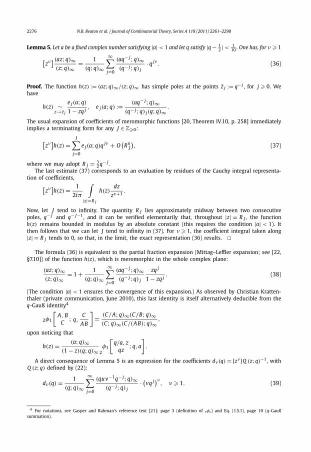
Lemma 5. Let a be a fixed complex number satisfying |a| < 1 and let q satisfy |q − 12 | < 1
10 . One has, for ν � 1[zν
] (az;q)∞(z;q)∞
= 1
(q;q)∞
∞∑j=0
(aq− j;q)∞(q− j;q) j
· q jν . (36)
Proof. The function h(z) := (az;q)∞/(z;q)∞ has simple poles at the points z j := q− j , for j � 0. Wehave
h(z) ∼z→z j
e j(a;q)
1 − zq j, e j(a;q) := (aq− j;q)∞
(q− j;q) j(q;q)∞.
The usual expansion of coefficients of meromorphic functions [20, Theorem IV.10, p. 258] immediatelyimplies a terminating form for any J ∈ Z�0:
[zν
]h(z) =
J∑j=0
e j(a;q)q jν + O(
RnJ
), (37)
where we may adopt R J = 32 q− J .
The last estimate (37) corresponds to an evaluation by residues of the Cauchy integral representa-tion of coefficients,[
zν]h(z) = 1
2iπ
∫|z|=R J
h(z)dz
zν+1.
Now, let J tend to infinity. The quantity R J lies approximately midway between two consecutivepoles, q− J and q− J−1, and it can be verified elementarily that, throughout |z| = R J , the functionh(z) remains bounded in modulus by an absolute constant (this requires the condition |a| < 1). Itthen follows that we can let J tend to infinity in (37). For ν � 1, the coefficient integral taken along|z| = R J tends to 0, so that, in the limit, the exact representation (36) results. �
The formula (36) is equivalent to the partial fraction expansion (Mittag–Leffler expansion; see [22,§7.10]) of the function h(z), which is meromorphic in the whole complex plane:
(az;q)∞(z;q)∞
= 1 + 1
(q;q)∞
∞∑j=0
(aq− j;q)∞(q− j;q) j
zq j
1 − zq j. (38)
(The condition |a| < 1 ensures the convergence of this expansion.) As observed by Christian Kratten-thaler (private communication, June 2010), this last identity is itself alternatively deducible from theq-Gauß identity4
2φ1
[A, B
C; q,
C
AB
]= (C/A;q)∞(C/B;q)∞
(C;q)∞(C/(AB);q)∞,
upon noticing that
h(z) = (a;q)∞(1 − z)(q;q)∞ 2
φ1
[q/a, z
qz;q,a
].
A direct consequence of Lemma 5 is an expression for the coefficients dν(q) = [zν ]Q (z;q)−1, withQ (z;q) defined by (22):
dν(q) = 1
(q;q)∞
∞∑j=0
(quv−1q− j;q)∞(q− j;q) j
· (vq j)ν, ν � 1. (39)
4 For notations, see Gasper and Rahman’s reference text [21]: page 3 (definition of rφs) and Eq. (1.5.1), page 10 (q-Gaußsummation).

N.R. Beaton et al. / Journal of Combinatorial Theory, Series A 118 (2011) 2261–2290 2277
To see this, set
a = quv−1 = q2
1 − q + q2,
and replace z by zv in the definition of h(z). Note that at q = 1/2, we have u = 1, v = 3/2, a = 1/3,so that, for q ≈ 1/2, we expect dν(q) to grow roughly like (3/2)ν .
Summarizing the results obtained so far, we state:
Proposition 3. The generating function of 3-sided prudent polygons satisfies the identity
PA(q) = D(q) − q2 A(q)(a;q)∞(v;q)∞(q;q)∞(av;q)∞
∞∑ν=1
∞∑j=0
[(aq− j;q) j
(q− j;q) j· vνq( j+1)ν
1 − 2q + qν+2
], (40)
where
a = q2
1 − q + q2, v = 1 − q + q2
1 − q, D(q) = C(q) − q2
(1 − q)2A(q)
(v;q)∞(av;q)∞
, (41)
and A(q), C(q) are rational functions defined in Eq. (21).
Proof. The identity is a direct consequence of the formula (39) for dν(q) and of the expressionfor PA(q) in (34), using the equivalence av = qu and the simple reorganization(
aq− j;q)∞ = (
aq− j;q)
j · (a;q)∞.
Previous developments imply that the identity (40) is, in particular, valid in the real interval (0, 12 ).
The trivial equality
(aq− j;q) j
(q− j;q) j= (a − q)(a − q2) · · · (a − q j)
(1 − q)(1 − q2) · · · (1 − q j)(42)
then shows that the expression on the right-hand side indeed represents a bona fide formal powerseries in q, since the q-valuation of the general term of the double sum in (40) increases with both jand ν . �
The formula (40) of Proposition 3 will serve as the starting point of the asymptotic analysis ofPA(q) as q → 1/2 in the next subsection. Given the discussion of the analyticity of the various com-ponents in the proof of Lemma 3, the task essentially reduces to estimating the double sum in asuitable complex neighborhood of q = 1/2.
3.2. Mellin analysis
Let T (q) be the double sum that appears in the expression (40) of PA(q). We shall take it here inthe form
T =∞∑j=0
(aq− j;q) j
(q− j;q) jH j(q) where H j(q) :=
∞∑ν=1
vνq( j+1)ν
1 − 2q + qν+2. (43)
We will now study the functions H j and propose to show that those of greater index contributeless significant terms in the asymptotic expansion of PA(q) near q = 1/2. In this way, a completeasymptotic expansion of the function PA(q), hence of its coefficients PAn , can be obtained.
The main technique used here is that of Mellin transforms: we refer the reader to [17] for detailsof the method. The principles are recalled in Section 3.2.1 below. We then proceed to analyze thedouble sum T of (43) when q is real and q tends to 1/2. The corresponding expansion is fairlyexplicit and it is obtained at a comparatively low computational cost in Section 3.2.2. We finally showin Section 3.2.3 that the expansion extends to a sector of the complex plane around q = 1/2.

2278 N.R. Beaton et al. / Journal of Combinatorial Theory, Series A 118 (2011) 2261–2290
3.2.1. Principles of the Mellin analysisLet f (x) be a complex function of the real argument x. Its Mellin transform, denoted by f �(s) or
M[ f ], is defined as the integral
M[ f ](s) ≡ f �(s) :=∞∫
0
f (x)xs−1 dx, (44)
where s may be complex. It is assumed that f (x) is locally integrable. It is then well known that if fsatisfies the two asymptotic conditions
f (x) =x→0
O(xα
), f (x) =
x→+∞ O(xβ
),
with α > β , then f � is an analytic function of s in the strip of the complex plane,
−α < �(s) < −β,
also known as a fundamental strip. Then, with c any real number of the interval (−α,−β), the follow-ing inversion formula holds (see [38, §VI.9] for detailed statements):
f (x) = 1
2iπ
c+i∞∫c−i∞
f �(s)x−s ds. (45)
There are then two essential properties of Mellin transforms.
(M1) Harmonic sum property. If the pairs (λ,μ) range over a denumerable subset of R×R>0 then onehas the equality
M[ ∑
(λ,μ)
λ f (μx)
]= f �(s) ·
( ∑(λ,μ)
λμ−s)
. (46)
That is to say, the harmonic sum∑
λ f (μx) has a Mellin transform that decomposes as aproduct involving the transform of the base function ( f �) and the generalized Dirichlet se-ries (
∑λμ−s) associated with the “amplitudes” λ and the “frequencies” μ. Detailed validity
conditions, spelled out in [17], are that the exchange of summation (∑
, in the definition of theharmonic sum) and integral (
∫, in the definition of the Mellin transform) be permissible.
(M2) Mapping properties. Poles of transforms are in correspondence with asymptotic expansions ofthe original function. More precisely, if the Mellin transform F � of a function F admits a mero-morphic extension beyond the fundamental strip, with a pole of some order m at some points0 ∈ C, with �(s0) < −α, then it contributes an asymptotic term of the form P (log x)x−s0 in theexpansion of F (x) as x → 0, where P is a computable polynomial of degree m − 1. Schemati-cally:
F �(s) :s→s0
C
(s − s0)m ⇒ F (x) :
x→0P (log x)x−s0 = Res
(f �(s)x−s)
s=s0. (47)
Detailed validity conditions, again spelled out in [17], are a suitable decay of the transformF �(s), as �(s) → ±∞, so as to permit an estimate of the inverse Mellin integral (45) byresidues — in (47), the expression is then none other than the residue of f �(s)x−s at s = s0.
The power of the Mellin transform for the asymptotic analysis of sums devolves from the appli-cation of the mapping property (M2) to functions F (x) = ∑
λ f (μx) that are harmonic sums in thesense of (M1). Indeed, the factorization property (46) of (M1) makes it possible to analyze separatelythe singularities that arise from the base function (via f �) and from the amplitude–frequency pairs(via
∑λμ−s); hence an asymptotic analysis results, thanks to (M2).

N.R. Beaton et al. / Journal of Combinatorial Theory, Series A 118 (2011) 2261–2290 2279
3.2.2. Analysis for real values of q → 1/2Our purpose now is to analyze the quantity T of (43) with q < 1/2, when q → 1/2. This basically
reduces to analyzing the quantities H j(q) of (43). Our approach consists of setting t = 1 − 2q anddecoupling5 the quantities t and q. Accordingly, we define the function
h j(t) ≡ h j(t;q, v) := q−2∞∑
ν=1
(vq j)ν
1 + tq−ν−2, (48)
so that
H j(q) = h j(t;q, v(q)
),
with the definition (43). We shall let t range over R�0 but restrict the parameter q to a small interval(1/2 − ε0,1/2 + ε0) of R and the parameter v to a small interval of the form (3/2 − ε1,3/2 + ε1),since v(1/2) = 3/2. We shall write such a restriction as
q ≈ 1
2, v ≈ 3
2,
with the understanding that ε0, ε1 can be taken suitably small, as the need arises. Thus, for the timebeing, we ignore the relations that exist between t and the pair q, v, and we shall consider them as independentquantities.
As a preamble to the Mellin analysis, we state an elementary lemma.
Lemma 6. Let q be restricted to a sufficiently small interval containing 1/2 and v to a sufficiently small intervalcontaining 3/2. Each function h j(t) defined by (48) satisfies the estimate
h j(t) =t→+∞ O
(1
t
), h j(t) =
t→0
{O (1) if j � 1,
O (t−γ ) if j = 0, with γ = log vlog(1/q)
.(49)
For γ , we can also adopt any fixed value larger than log2(4/3).= 0.415, provided q and v are taken
close enough to 1/2 and 3/2, respectively.
Proof. Behavior as t → +∞. The inequality (1 + tq−ν−2)−1 < t−1qν+2 implies by summation the in-equality
h j(t) � q−2t−1∞∑
ν=1
vνq jνqν = O
(1
t
), t → +∞,
given the convergence of the geometric series∑
ν vq( j+1)ν , for v ≈ 3/2 and q ≈ 1/2.Behavior as t → 0. First, for the easy case j � 1, the trivial inequality (1 + tq−ν−2)−1 � 1 implies
h j(t) = O
(∑ν
(vq j)ν)
= O (1), t → 0.
Next, for j = 0, define the function
ν0(t) := −2 + log(1/t)
log(1/q),
so that tq−ν−2 < 1, if ν < ν0(t), and tq−ν−2 � 1, if ν � ν0(t). Write∑
ν = ∑ν0
+∑ν�ν0
. The sumcorresponding to ν � ν0 is bounded from above as in the case of t → +∞,∑
ν�ν0(t)
vν
1 + tq−ν−2�
∑ν�ν0(t)
vνt−1qν+2 = O(t−1(vq)ν0
) = O(t−1(vq)ν0
), t → 0,
5 An instance of such a decoupling technique appears for instance in de Bruijn’s reference text [5, p. 27].

2280 N.R. Beaton et al. / Journal of Combinatorial Theory, Series A 118 (2011) 2261–2290
and the last quantity is O (t−γ ) for γ = (log v)/ log(1/q). The sum corresponding to ν < ν0 is dom-inated by its later terms and is accordingly found to be O (t−γ ). The estimate of h0(t), as t → 0,results. �
We can now proceed with a precise asymptotic analysis of the functions h j(t), as t → 0. Lemma 6implies that each h j(t) has its Mellin transform h�
j(s) that exists in a non-empty fundamental stripleft of �(s) = 1. In that strip, the Mellin transform is
M[h j(t)
] = q−2 M[
1
1 + t
]·( ∞∑
ν=1
(vq j)ν(
q−ν−2)−s
)(by the harmonic sum property (M1)
)= q−2 M
[1
1 + t
]· vq j+3s
1 − vq j+s(by summation of a geometric progression)
= q−2 π
sinπ s
vq j+3s
1 − vq j+s
(by the classical form of M
[(1 + t)−1
]). (50)
The Mellin transform of (1 + t), which equals π/ sin(π s), admits 0 < �(s) < 1 as the fundamen-tal strip, so this condition is necessary for the validity of (50). In addition, the summability of theDirichlet series, here plainly a geometric series, requires the condition |vq j+s| < 1; that is,
�(s) > − j + log v
log 1/q.
In summary, the validity of (50) is ensured for s satisfying
λ < �(s) < 1, with λ := max
(0,− j + log v
log 1/q
).
Lemma 7. For q ≈ 1/2 and v ≈ 3/2 restricted as in Lemma 6, the function h j(t) admits an exact representa-tion, valid for any t ∈ (0,q−3),
h j(t) = (−1) j vq3γ −2 j−2
log 1/qt j−γ Π(log1/q t) + q−2
∑r�0
(−1)r vq j−3r
1 − vq j−rtr . (51)
Here,
γ ≡ γ (q) := log v
log 1/q
so that γ ≈ log232
.= 0.415, when q ≈ 12 ; the quantity Π(u) is an absolutely convergent Fourier series,
Π(u) :=∑k∈Z
pke−2ikπu, (52)
with coefficients pk given explicitly by
pk = π
sin(πγ + 2ikπ2/(log 1/q)). (53)
Observe that the pk decrease geometrically with k. For instance, at q = 1/2, one has
pk = O(e−2kπ2/ log 2) .= O
(4.28 · 10−13)k
, (54)
as is apparent from the exponential form of the sine function. Consequently, even the very first coef-ficients are small: at q = 1/2, typically,
|p1| = |p−1| .= 2.69 · 10−12, |p2| = |p−2| .= 1.15 · 10−24, |p3| = |p−3| .= 4.95 · 10−37.

N.R. Beaton et al. / Journal of Combinatorial Theory, Series A 118 (2011) 2261–2290 2281
Proof of Lemma 7. We first perform an asymptotic analysis of h j(t) as t → 0+ . This requires thedetermination of poles to the left of the fundamental strip of h�
j(s), and these arise from two sources.
– The relevant poles of π/ sinπ s are at s = 0,−1,−2, . . . ; they are simple and the residue at s = −ris (−1)r .
– The quantity (1 − vq j+s)−1 has a simple pole at the real point
σ0 := − j + log v
log 1/q, (55)
as well as complex poles of real part σ0, due to the complex periodicity of the exponential function(et+2iπ = et ). The set of all poles of (1 − vq j+s)−1 is then{
σ0 + 2ikπ
log 1/q, k ∈ Z
}.
The proof of an asymptotic representation (that is, of (51), with ‘∼’ replacing the equality signthere) is classically obtained by integrating h�
j(s)t−s along a long rectangle with corners at −d − iTand c + iT , where c lies within the fundamental strip (in particular, between 0 and 1) and d will betaken to be of the form −m − 1
2 , with m ∈ Z�0, and smaller than − j +γ . In the case considered here,there are regularly spaced poles along �(s) = − j + γ , so that one should take values of T that aresuch that the line �(s) = T passes half-way between poles. This, given the fast decay of π/ sinπ s as|�(s)| increases and the boundedness of the Dirichlet series (1 − vq j+s)−1 along �(s) = ±T , allowsus to let T tend to infinity. By the Residue Theorem applied to the inverse Mellin integral (45), wecollect in this way the contribution of all the poles at − j + γ + 2ikπ/(log 1/q), with k ∈ Z, as well asthe m + 1 initial terms of the sum
∑r in (51). The resulting expansion is of type (51) with the sum∑
r truncated to m + 1 terms and an error term that is O (tm+1/2).In general, what the Mellin transform method gives is an asymptotic rather than exact representa-
tion of this type. Here, we have more. We can finally let m tend to infinity and verify that the inverseMellin integral (45) taken along the vertical line �(s) = −m − 1
2 remains uniformly bounded in mod-ulus by a quantity of the form ctmq−3m , for some c > 0. In the limit m → +∞, the integral vanishes(as long as tq−3 < 1), and the exact representation (51) is obtained. �
We can now combine the identity provided by Lemma 7 with the decomposition of the gen-erating function PA(q) as allowed by Eq. (43), which flows from Proposition 3. We recall thatH j(q) = h j(t;q, v(q)).
Proposition 4. The generating function PA(q) of prudent polygons satisfies, for q in a small enough interval6
of the form (1/2 − ε,1/2) (for some ε > 0), the identity
PA(q) = D(q) − q2 A(q)(a;q)∞(v;q)∞(q;q)∞(av;q)∞
T (q), (56)
where the notations are those of Proposition 3, and the function T (q) admits the exact representation
T (q) = (1 − 2q)−γ · Π(
log(1 − 2q)
log 1/q
)U (q) + V (q), γ ≡ log v
log 1/q, (57)
with Π(u) given by Lemma 7, Eqs. (52) and (53). Set
t = 1 − 2q.
The “singular series” U (q) is
U (q) = vq3γ −2
log 1/q
(−q−1t;q)∞(−aq−2t;q)∞
, γ = log v
log 1/q; (58)
6 Numerical experiments suggest that in fact the formula (57) remains valid for all q ∈ (0,1/2).

2282 N.R. Beaton et al. / Journal of Combinatorial Theory, Series A 118 (2011) 2261–2290
and the “regular series” V (q) is
V (q) = − (q;q)∞(a;q)∞
q−2
1 + q−2t+ q−2 (q;q)∞(av;q)∞
(a;q)∞(v;q)∞
∞∑r=0
(a−1 v−1q;q)r
(v−1q;q)r
(−aq−2t)r
. (59)
Proof. We start from T (q) as defined by (43). The q-binomial theorem is the identity [21, §1.3]
(θ z;q)∞(z;q)∞
=∞∑
n=0
(θ;q)n
(q;q)nzn. (60)
Now consider the first term in the expansion (51) of Lemma 7. Sum the corresponding contribu-tions for all values of j � 0, after multiplication by the coefficient (aq− j;q) j/(q− j;q) j , in accordancewith (43). This gives
U (q) = vq3γ −2
log 1/q
∞∑j=0
(aq− j;q) j
(q− j;q) j
(−q2t) j = vq3γ −2
log 1/q
∞∑j=0
(a−1q;q) j
(q;q) j
(−aq−2t) j
which provides the expression for U (q) of the singular series, via the q-binomial theorem (60) takenwith z = −at and θ = a−1q.
Summing over j in the second term in the identity (51) of Lemma 7, we have
V (q) = q−2∞∑
r=0
(−q−2t)r
∞∑j=0
(aq− j;q) j
(q− j;q) j
vq j−r
1 − vq j−r.
Now, the Mittag–Leffler expansion (38) associated with Lemma 5 can be put in the form
(az;q)∞(z;q)∞
= 1 + (a;q)∞(q;q)∞
∞∑j=0
(aq− j;q) j
(q− j;q) j
zq j
1 − zq j.
An application of this identity to V (q), with z = vq−r , shows that
V (q) = q−2 (q;q)∞(a;q)∞
∞∑r=0
(−q−2t)r
((avq−r;q)∞(vq−r;q)∞
− 1
),
which is equivalent to the stated form of V (q). Note that this last form is a q-hypergeometric functionof type 2φ1; see [21].
So far, we have proceeded formally and left aside considerations of convergence. It can be easilyverified that all the sums, single or double, involved in the calculations above are absolutely (anduniformly) convergent, provided t is taken small enough (i.e., q is sufficiently close to 1/2), giventhat all the involved parameters, such as a, u, v , then stay in suitably bounded intervals of the realline. �3.2.3. Analysis for complex values of q → 1/2
We now propose to show that the “transcendental” expression of PA(q) provided by Proposition 4is actually valid in certain regions of the complex plane that extend beyond an interval of the realline. The regions to be considered are dictated by the requirements of the singularity analysis methodto be deployed in the next subsection.
Definition 3. Let θ0 be a number in the interval (0,π/2), called the angle, and r0 a number in R>0 , called theradius. A sector (anchored at 1/2) is comprised of the set of all complex numbers z = 1/2 + reiθ such that
0 < r < r0 and θ0 < θ < 2π − θ0.

N.R. Beaton et al. / Journal of Combinatorial Theory, Series A 118 (2011) 2261–2290 2283
We stress the fact that the angle should be strictly smaller than π/2, so that a sector in the senseof the definition always includes a part of the line �(s) = 1/2. The smallness of a sector will bemeasured by the smallness of r0. That is to say:
Proposition 5. There exists a sector S0 (anchored at 1/2), of angle7 θ0 < π/2 and radius r0 > 0, such thatthe identity expressed by Eqs. (56) and (57) holds for all q ∈ S0 .
Proof. The proof is a simple consequence of analytic continuation. We first observe that an infiniteproduct such as (c;q)∞ is an analytic function of both c and q, for arbitrary c and |q| < 1. Similarly,the inverse 1/(c;q)∞ is analytic provided cq j �= 1, for all c. For instance, taking c = a where a = a(q) =q2/(1 − q + q2) and noting that a(1/2) = 1/3, we see that 1/(a;q) is an analytic function of q in asmall complex neighborhood of q = 1/2. This reasoning can be applied to the various Pochhammersymbols that appear in the definition of T (q), U (q), V (q). Similarly, the hypergeometric sum thatappears in the regular series V (q) is seen to be analytic in the three quantities a ≈ 1/3, v ≈ 3/2,and t = 1 − 2q ≈ 0. In particular, the functions U (q) and V (q) are analytic in a complex neighborhood ofq = 1/2.
Next, consider the quantity
(1 − 2q)−γ = exp(−γ log(1 − 2q)
).
The function γ ≡ γ (q) is analytic in a neighborhood of q = 1/2, since it equals (log v)/(log 1/q). Thelogarithm, log(1 − 2q), is analytic in any sector anchored at 1/2. By composition, there results that(1 − 2q)−γ is analytic in a small sector anchored at 1/2. It only remains to consider the Π factorin (56). A single Fourier element, pke−2ikπu , with u = log1/q t and t = 1 − 2q, is also analytic in asmall sector (anchored at 1/2), as can be seen from the expression
pke−2ikπu = pk exp
(−2ikπ
log(1 − 2q)
log 1/q
). (61)
Note that, although �(log(1 − 2q)) → ∞ as q → 1/2, the complex exponential exp(2ikπ log2(1 − 2q))
remains uniformly bounded, since �(log(1 − 2q)) is bounded for q in a sector. Then, given the fastgeometric decay of the coefficients pk at q = 1/2 (namely, pk = O (e−2kπ2/ log 2); cf. (53)), it followsthat Π(log2 t) is also analytic in a sector. A crude adjustment of this argument (see (70) and (71)below for related expansions) suffices to verify that the geometric decay of the terms composing (61)persists in a sector anchored at 1/2, so that Π(log1/q t) is also analytic in such a sector.
Finally, the auxiliary quantities D(q), A(q) are meromorphic at q = 1/2, with at most a doublepole there; in particular, they are analytic in a small enough sector anchored at 1/2. We can thenchoose for S0 a small sector that satisfies this as well as all the previous analyticity constraints. Then,by unicity of analytic continuation, the expression on the right-hand side of (56), with T (q) as givenby (57), must coincide with (the analytic continuation of) PA(q) in the sector S0. �3.3. Singularity analysis and transfer
If we drastically reduce all the non-singular quantities that occur in the main form (56) of Propo-sition 4 by letting q → 1/2, we are led to infer that PA(q) satisfies, in a sector around q = 1/2, anestimate of the form
PA(q) = ξ0(1 − 2q)−γ0−2Π(log2(1 − 2q)
) + O((1 − 2q)−3/2), γ0 := log2(3/2), (62)
where
ξ0 = − 1
16U (1/2)
(1/3;1/2)∞(3/2;1/2)∞(1/2;1/2)∞(1/2;1/2)∞
, U (1/2) = 16
9 log 2, (63)
7 A careful examination of the proof of Proposition 5 shows that any angle θ0 > 0, however small, is suitable, but only theexistence of some θ0 < π/2 is needed for singularity analysis.

2284 N.R. Beaton et al. / Journal of Combinatorial Theory, Series A 118 (2011) 2261–2290
and U (q) is the singular series of (58). Let us ignore for the moment the oscillating terms and simplifyΠ(u) to its constant term p0, with pk given by (53). This provides a numerical approximation PA(q)
of PA(q). With the general asymptotic approximation (derived from Stirling’s formula)[qn](1 − 2q)−λ ∼
n→+∞1
�(λ)2nnλ−1, λ /∈ Z�0, (64)
it is easily seen that [qn]PA(q) is asymptotic to the quantity κ02nng of Eq. (18) in Theorem 2, whichis indeed the “principal” asymptotic term of PAn = [qn]PA(q), where g = γ0 + 1 = log2 3.
A rigorous justification and a complete analysis depend on the general singularity analysis theory[20, Chapter VI] applied to the expansion of PA(q) near q = 1/2. We recall that a �-domain with base 1is defined to be the intersection of a disc of radius strictly larger than 1 and of the complement of asector of the form −θ0 < arg(z − 1) < θ0 for some θ0 ∈ (0,π/2). A �-domain with base ρ is obtainedfrom a �-domain with base 1 by means of the homothetic transformation z → ρz. Singularity analysistheory is then based on two types of results.
(S1) Coefficients of functions in a basic asymptotic scale have known asymptotic expansions [20, The-orem VI.1, p. 381]. In the case of the scale (1 − z)−λ , the expansion, which extends (64), is of theform [
zn](1 − z)−λ ∼n→+∞nλ−1
(1 +
∑k�1
ek
nk
), λ ∈ C \ Z�0,
where ek is a computable polynomial in λ of degree 2k. Observe that this expansion is valid forcomplex values of the exponent λ, and if λ = σ + iτ , then
nλ−1 = nσ−1 · niτ = nσ−1eiτ log n.
Thus, the real part (σ ) of the singular exponent drives the asymptotic regime; the imaginarypart, as soon as it is non-zero, induces periodic oscillations in the scale of log n. A noteworthyfeature is that smaller functions at the singularity z = 1 have asymptotically smaller coefficients.
(S2) An approximation of a function near its singularity can be transferred to an approximation ofcoefficients according to the rule
f (z) =z→1
O((1 − z)−λ
) ⇒ [zn] f (z) =
n→+∞ O(nλ−1).
The condition is that f (z) be analytic in a �-domain and that the O -approximation holds insuch a �-domain, as z → 1; see [20, Theorem VI.3, p. 390]. Once more, smaller error terms areassociated with smaller coefficients.
Equipped with these principles, it is possible to obtain a complete asymptotic expansion of [qn]PA(q)
once a complete expansion of PA(q) in the vicinity of q = 1/2 has been obtained (set q = z/2, so thatz ≈ 1 corresponds to q = 1/2). In this context, Proposition 3 precisely grants us the analytic continua-tion of PA(q) in a �-domain anchored at 1/2, with any opening angle arbitrarily small; Proposition 4,together with Proposition 5, describes in a precise manner the asymptotic form of PA(q) as q → 1/2in a �-domain and it is a formal exercise to transform them into a standard asymptotic expansion, inthe form required by singularity analysis theory.
Proposition 6. As q → 1/2 in a �-domain, the function PA(q) satisfies the expansion
PA(q) ∼q→1/2
1
(1 − 2q)+ R(q) +
∑j�1
(1 − 2q)−γ0−2+ jj∑
�=0
(log(1 − 2q)
)�Π( j,�)(log2(1 − 2q)
),
γ0 = log23. (65)
2
N.R. Beaton et al. / Journal of Combinatorial Theory, Series A 118 (2011) 2261–2290 2285
Here R(q) is analytic at q = 1/2 and each Π( j,�)(u) is a Fourier series
Π( j,�)(u) :=∑k∈Z
p( j,�)k e2ikπu,
with a computable sequence of coefficients p( j,�)k .
Proof. From Proposition 4, we have
PA(q) = PAreg(q) + PAsing(q), (66)
where the two terms correspond, respectively, to the “regular” part (involving the regular series V (q))and the “singular part” (involving the singular series U (q) as well as the factor (1 − 2q)−γ and theoscillating series).
Regarding the regular part, we have, with the notations of Proposition 4,
PAreg(q) = D(q) − q2 A(q)(a;q)∞(v;q)∞(q;q)∞(q;q)∞
V (q). (67)
We already know that A(q) and D(q) are meromorphic at q = 2 with a double pole, while V (q)
and the Pochhammer symbols are analytic at q = 1/2. Thus, this regular part has at most a doublepole at q = 1/2. A simple computation shows that the coefficient of (1 − 2q)−2 reduces algebraicallytrivially — in the sense that no q-identity is involved — to 0. Thus, the regular part involves only asimple pole at q = 1/2, as is expressed by the first two terms of the expansion (66), where R(q) isanalytic at q = 1/2. (Note that the coefficient of (1 − 2q)−1 is exactly 1, again for trivial reasons.)
The singular part is more interesting and it can be analyzed by the method suggested at thebeginning of this subsection. Whenever convenient, we freely use the abbreviation t = 1 − 2q. Thefunction γ (q) = (log v)/(log 1/q) is analytic at q = 1/2, where
γ (q) = log23
2+ 2
log 3
(log 2)2
(q − 1
2
)+ · · ·
.= 0.58496 + 4.5732
(q − 1
2
)+ 16.317
(q − 1
2
)2
+ 39.982
(q − 1
2
)3
+ 86.991
(q − 1
2
)4
+ · · · .
The function (1 − 2q)−γ can then be expanded as
(1 − 2q)−γ (q) = (1 − 2q)−γ0 e−(γ (q)−γ0) log t, with γ0 = γ (1/2) = log23
2
= (1 − 2q)−γ0
(1 + log 3
(log 2)2t log t + t2 P2(log t) + t3 P3(log t) + · · ·
), (68)
for a computable family of polynomials P2, P3, . . . , where deg P� = � and P�(0) = 0. For instance, wehave, with y := log t:
(1 − 2q)−(γ −γ0) log t .= 1 + 2.28ty + t2(−4.07y + 2.61y2) + t3(4.99y − 9.32y2 + 1.99y3)+ · · · .
The singular series U (q) of (58) is analytic at q = 1/2 and its coefficients can be determined, bothnumerically and, in principle, symbolically in terms of Pochhammer symbols and their logarithmicderivatives (which lead to q-analogues of harmonic numbers). Numerically, they can be estimated tohigh precision, by bounding the infinite sum and products to a finite but large value. (The validityof the process can be checked empirically by increasing the values of this threshold, the justificationbeing that all involved sums and products converge geometrically fast — we found that replacing +∞

2286 N.R. Beaton et al. / Journal of Combinatorial Theory, Series A 118 (2011) 2261–2290
by 100 in numerical computations provides estimates that are at least correct to 25 decimal digits.) Inthis way, we obtain, for instance, the expansion of the function V (q), which is of the form (t = 1−2q)
U (q).= 16
9 log 2+ 9.97t + 21.5t2 + 35.8t3 + 51.9t4 + · · · . (69)
Finally, regarding Π(u) taken at u = log1/q(1 − 2q), we note that the coefficients pk of (53) can be
expanded around q = 1/2 and pose no difficulty, while the quantities e2ikπu can be expanded by aprocess analogous to (68). Indeed, we have
pk ≡ pk(q) = π
sin(πγ0 + 2ikπ2/ log 2)· exp
(1 + e1(k)t + e2(k)t2 + · · ·), (70)
where the ek only grow polynomially with k. Also, at u = log1/q(1 − 2q), one has
e2ikπu = (1 − 2q)2ikπ/ log 2 exp[2ikπ log2 t
(g1t + g2t2 + · · ·)], (71)
where the coefficients g j are those of (log 1/q)−1 − (log 2)−1 expanded at q = 1/2 and expressed interms of t = 1 − 2q.
We can now recapitulate the results of the discussion of the singular part: from (69), (70), and (71),we find that the terms appearing in the singular expansion of PA(q) are of the form, for j = 0,1,2, . . . ,
(1 − 2q)−γ0−2t j(log t)�t2ikπ/ log 2,
with � such that 0 � � � j and k ∈ Z. The terms at fixed j, � add up to form the Fourier series Π( j,�) ,whose coefficients exhibit a fast decrease with |k|, similar to that encountered in (54). Consequently,a finite version of (65) at any order holds, so that the statement results. �
With this last proposition, we can conclude the proof of Theorem 2.
Proof of Theorem 2. The analytic term R(q) in (65) leaves no trace in the asymptotic form of co-efficients. Thus the global contribution of the regular part to coefficients PAn reduces to 2n (withcoefficient 1 and no power of n), corresponding to the term (1 − 2q)−1 in (65).
The transfer to coefficients of each term of the singular part of (65) is permissible, given the prin-ciples of singularity analysis recalled above. Only an amended form allowing for logarithmic factors isneeded, but this is covered by the general theory: for the translation of the coefficients of the basicscale (1− z)−λ logk(1− z), see [20, p. 387]. From a computational point of view, one may convenientlyoperate [20, Note VI.7, p. 389] with[
zn](1 − z)−λ(log(1 − z)
)k = (−1)k ∂
∂λ
�(n + λ)
�(λ)�(n + 1),
then replace the Gamma factors of large argument by their complete Stirling expansion.We can now complete the proof of Theorem 2. It suffices simply to retain the terms corresponding
to j = 0 in (65), in which case the error term becomes of the form O ((1 − 2q)−γ0−1 log(1 − 2q)),which corresponds to a contribution that is O (nγ0 logn) = O (ng−1 log n) for PAn .
Next, regarding the Fourier element of index k = 0, the function-to-coefficient correspondenceyields
(1 − 2q)−γ0−2 ⇒ nγ0+1
�(γ0 + 2)
(1 + O
(1
n
)).
Thus, the coefficient κ0 in (19) has value (cf. (62) and (63)) given by
κ0 = ξ0 · p0|q=1/2 · 1
�(γ0 + 2), γ0 = log 3/2
log 2,
with ξ0 as in (63). This, given the form (53) of pk at k = 0, is equivalent to the value of κ0 stated inTheorem 2 (where g := γ0 + 1 = log2 3).

N.R. Beaton et al. / Journal of Combinatorial Theory, Series A 118 (2011) 2261–2290 2287
For a Fourier element of index k ∈ Z , we have similarly
(1 − 2q)−γ0−2−iχk ⇒ nγ0+1+iχk
�(γ0 + 2 + iχk)
(1 + O
(1
n
)), where χk := 2kπ
log 2.
We finally observe that
nγ0+1+iχk = nγ0+1eiχk log n,
so that all the terms, for k ∈ Z, are of the same asymptotic order (namely, O (nγ0+1)) and their sumconstitutes a Fourier series in log n. The Fourier coefficient κk then satisfies, from the discussionabove:
κk = ξ0 · pk|q=1/2 · 1
�(γ0 + 2 + iχk).
Thus finally, with g ≡ γ0 + 1:
κk = π
9 log 2 sin(π g + 2ikπ2/ log 2)�(g + 1 + 2ikπ/ log 2)
∞∏j=0
(1 − 13 2− j)(1 − 3
2 2− j)
(1 − 12 2− j)2
. (72)
This completes the proof of Theorem 2. �The same method shows the existence of a complete asymptotic expansion for PAn .
Theorem 3. The number of 3-sided prudent polygons satisfies a complete asymptotic expansion,
PAn ∼ 2n + 2n · ng(
Ξ0,0 + 1
n(log n · Ξ1,1 + Ξ1,0)
+ 1
n2
(log2 n · Ξ2,2 + logn · Ξ2,1 + Ξ2,0
) · · ·)
,
where Ξ j,� is an absolutely convergent Fourier series in log n.
The non-oscillating form obtained by retaining only the constant terms of each Fourier series iscomputed by a symbolic manipulation system such as Maple or Mathematica in a matter of secondsand is found to start as
Ω5
2n.= 1 + 0.1083842947 · ng + (−0.3928066917L + 0.5442458535) · ng−1
+ (0.2627062704L2 + 0.6950193894L + 0.6985601031
) · ng−2
+ (0.08310555463L3 − 0.02188678892L2 − 1.570478457L
− 1.18810811075202) · ng−3
+ (0.06722511293L4 + 0.05494834609L3 − 3.297513638L2 − 4.663711650L
− 4.156441653) · ng−4, (73)
where L = log n. In principle, all the coefficients have explicit forms in terms of the basic quantitiesthat appear in Theorem 2 (augmented by derivatives of q-Pochhammer symbols at small rationalvalues). However, the corresponding formulae blow up exponentially, so that we only mention herethe next coefficient −0.39280 . . . in (73), whose exact value turns out to be
−κ0log 3
log2 2g.
Fig. 6 displays the difference between PAn and the six-term extension Ω6 of (73). It is piquant tonote that all the terms given in Eq. (73) are needed in order to succeed in bringing the fluctuations
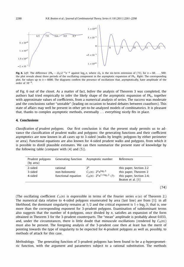
2288 N.R. Beaton et al. / Journal of Combinatorial Theory, Series A 118 (2011) 2261–2290
Fig. 6. Left: The difference (PAn − Ω6)2−nn−g against log2 n, where Ω6 is the six-term extension of (73), for n = 60, . . . ,500;the plot reveals about three periods of the oscillating component in the asymptotic expansion of PAn . Right: The correspondingplot, for values up to n = 6000. The diagrams confirm the presence of oscillations that, asymptotically, have amplitude of theorder of 10−9.
of Fig. 6 out of the closet. As a matter of fact, before the analysis of Theorem 3 was completed, theauthors had tried empirically to infer the likely shape of the asymptotic expansion of PAn , togetherwith approximate values of coefficients, from a numerical analysis of series. The success was moderateand the conclusions rather “unstable” (leading on occasion to heated debates between coauthors). Thisstate of affairs may well be present in other yet-to-be-analyzed models of combinatorics. It is pleasantthat, thanks to complex asymptotic methods, eventually . . . everything nicely fits in place.
4. Conclusions
Classification of prudent polygons. Our first conclusion is that the present study permits us to ad-vance the classification of prudent walks and polygons: the generating functions and their coefficientasymptotics are now known in all cases up to 3-sided (walks by length; polygons by either perimeteror area). Functional equations are also known for 4-sided prudent walks and polygons, from which itis possible to distill plausible estimates. We can then summarize the present state of knowledge bythe following table (compare with (4) and (5)).
Prudent polygons Generating function Asymptotic number References(by area)
2-sided rational 2n this paper, Section 2.23-sided non-holonomic C3(n) · 2nnlog2 3 this paper, Theorem 24-sided functional equation C4(n) · 2nn1+log2 3 (?) this paper, Section 2.4;
Beaton et al. [1]
(74)
(The oscillating coefficient C3(n) is expressible in terms of the Fourier series κ(u) of Theorem 2.)The numerical data relative to 4-sided polygons enumerated by area (last line) are from [1]: in alllikelihood, the dominant singularity remains at 1/2 and the critical exponent is 1+ log2 3; that is, onemore than the corresponding exponent for 3-prudent polygons. Examination of subdominant termsalso suggests that the number of 4-polygons, once divided by n, satisfies an expansion of the formobtained in Theorem 3 for the 3-prudent counterparts. The “mean” amplitude is probably about 0.033,and, under the circumstances, there is little doubt that minuscule oscillations (rendered by C4(n))must also be present. The foregoing analysis of the 3-prudent case then at least has the merit ofpointing towards the type of singularity to be expected for 4-prudent polygons as well as, possibly, tomethods of attack for this case.
Methodology. The generating function of 3-prudent polygons has been found to be a q-hypergeomet-ric function, with the argument and parameters subject to a rational substitution. The methods

N.R. Beaton et al. / Journal of Combinatorial Theory, Series A 118 (2011) 2261–2290 2289
developed here should clearly be useful in a number of similar situations. Note that the asymp-totic enumeration of prudent walks and polygons by length and perimeter is in a way easier sincethe dominant singularity is polar or algebraic. (Bousquet-Mélou [3] however exhibits an interestingsituation where the complete singular structure has a complex geometry.)
Estimates involving periodic oscillations are not unheard of in combinatorial asymptotics [20,28,29]. What is especially interesting in the case of 3-sided prudent polygons is the pattern of singu-larities that accumulate geometrically fast to the dominant singularity. This situation is prototypicallyencountered in the already evoked problem of the longest run in strings: the classical treatment isvia real analytic methods followed by a Mellin analysis of the expressions obtained; see [25]. In fact,the chain
Coefficient asymptotics � Mellin transform + Singularity analysis (75)
is applicable for moment analyses. For instance, the analysis of the expected longest run of the let-ter a in a random binary sequence over the alphabet {a,b} leads to the generating function [20,Example V.4]
Φ(z) = (1 − z)∑k�0
zk
1 − 2z + zk+1,
to which the chain (75) can be applied.Another source of similar phenomena is the analysis of digital trees [26,35], when these are
approached via ordinary generating functions (rather than the customary exponential or Poissongenerating functions). Typically, in the simplest case of node-depth in a random digital tree, oneencounters the generating function
Ψ (z) = 1
1 − z
∑k�0
2−k
1 − z(1 − 2−k),
where the geometric accumulation of poles towards 1 is transparent, so that the chain (75) can oncemore be applied [19].
We should finally mention that “critical” exponents similar to g = log2 3 surface at several placesin mathematics, usually accompanied by oscillation phenomena, but they do so for reasons essentiallysimpler than in our chain (75). For instance, in fractal geometry, the Hausdorff dimension of the tri-adic Cantor set is 1/g , see [14], while that of the familiar Sierpinski gasket is g , so that g occurs ascritical exponent in various related integer sequences [18]. The same exponent g = log2 3 ≈ 1.58 isotherwise known to most students of computer science, since it appears associated to the recurrentsequence fn = n + 3 f�n/2� , which serves to describe the complexity of Karatsuba multiplication [27](where, recursively, the product of two double-precision numbers is reduced to three single-precisionnumbers). In such cases, the exponent g is eventually to be traced to the singularity (at s = g , pre-cisely) of the Dirichlet series
ω(s) = 1
1 − 3 · 2−s,
which is itself closely related to the Mellin transforms of our Eq. (50). See also the studies by Drmotaand Szpankowski [10], Dumas [12], as well as [18] for elements of a general theory.
For the various reasons evoked above, we believe that the asymptotic methods developed in thepresent paper are of a generality that goes somewhat beyond the mere case of 3-sided prudent poly-gons, and may illuminate other models of interest in lattice combinatorics and statistical mechanics.
References
[1] N.R. Beaton, P. Flajolet, A.J. Guttmann, The unusual asymptotics of 3-sided prudent polygons, J. Phys. A 43 (34) (2010)342001–342010.
[2] M. Bousquet-Mélou, A method for the enumeration of various classes of column-convex polygons, Discrete Math. 154(1996) 1–25.

2290 N.R. Beaton et al. / Journal of Combinatorial Theory, Series A 118 (2011) 2261–2290
[3] M. Bousquet-Mélou, Families of prudent self-avoiding walks, J. Combin. Theory Ser. A 117 (2010) 313–344.[4] M. Bousquet-Mélou, R. Brak, Exactly solved models of polyominoes and polygons, in: A.J. Guttmann (Ed.), Polygons, Poly-
ominoes and Polycubes, Chapter 3, in: Lecture Notes in Phys., vol. 775, Springer, 2009, pp. 43–78.[5] N.G. de Bruijn, Asymptotic Methods in Analysis, Dover, 1981, a reprint of the third North-Holland edition, 1970 (first
edition, 1958).[6] A.R. Conway, I.G. Enting, A.J. Guttmann, Algebraic techniques for enumerating self-avoiding walks on the square lattice,
J. Phys. A 26 (1993) 1519–1534.[7] M.-P. Delest, G. Viennot, Algebraic languages and polyominoes enumeration, Theoret. Comput. Sci. 34 (1984) 169–206.[8] J.C. Dethridge, T.M. Garoni, A.J. Guttmann, I. Jensen, Prudent walks and polygons, J. Phys. A 42 (2009) 1–16.[9] J.C. Dethridge, A.J. Guttmann, Prudent self-avoiding walks, Entropy 10 (3) (2008) 309–318.
[10] M. Drmota, W. Szpankowski, A master theorem for discrete divide and conquer recurrences, in: Proceedings of SODA 2011,p. 342, http://www.siam.org/proceedings/soda/2011/SODA11_028_drmotam.pdf.
[11] E. Duchi, On some classes of prudent walks, in: FPSAC’05, 2005.[12] P. Dumas, Mean asymptotic behaviour of radix-rational sequences and dilation equations (extended version), Tech. Rep.,
arXiv:0807.1523, 2008, 46 pp.
[13] H. Duminil-Copin, S. Smirnov, The connective constant of the honeycomb lattice equals√
2 + √2, Tech. Rep., arXiv:1007.
0575, 2010, 9 pp.[14] K.J. Falconer, The Geometry of Fractal Sets, Cambridge Tracts in Math., vol. 85, Cambridge University Press, 1985.[15] S. Finch, Mathematical Constants, Cambridge University Press, 2003.[16] P. Flajolet, S. Gerhold, B. Salvy, On the non-holonomic character of logarithms, powers, and the nth prime function, Electron.
J. Combin. 11 (2) (2005) 1–16.[17] P. Flajolet, X. Gourdon, P. Dumas, Mellin transforms and asymptotics: Harmonic sums, Theoret. Comput. Sci. 144 (1–2)
(June 1995) 3–58.[18] P. Flajolet, P. Grabner, P. Kirschenhofer, H. Prodinger, R. Tichy, Mellin transforms and asymptotics: Digital sums, Theoret.
Comput. Sci. 123 (2) (1994) 291–314.[19] P. Flajolet, B. Richmond, Generalized digital trees and their difference–differential equations, Random Structures Algo-
rithms 3 (3) (1992) 305–320.[20] P. Flajolet, R. Sedgewick, Analytic Combinatorics, Cambridge University Press, 2009.[21] G. Gasper, M. Rahman, Basic Hypergeometric Series, Encyclopedia Math. Appl., vol. 35, Cambridge University Press, 1990.[22] P. Henrici, Applied and Computational Complex Analysis, vol. 1, John Wiley, 1974.[23] I. Jensen, A.J. Guttmann, Self-avoiding polygons on the square lattice, J. Phys. A 32 (26) (1999) 4867–4876.[24] I. Jensen, A.J. Guttmann, Statistics of lattice animals (polyominoes) and polygons, J. Phys. A 33 (2000) L257–L263.[25] D.E. Knuth, The average time for carry propagation, Indag. Math. (N.S.) 40 (1978) 238–242.[26] D.E. Knuth, The Art of Computer Programming, vol. 3: Sorting and Searching, second ed., Addison–Wesley, 1998.[27] D.E. Knuth, The Art of Computer Programming, vol. 2: Seminumerical Algorithms, third ed., Addison–Wesley, 1998.[28] A.M. Odlyzko, Periodic oscillations of coefficients of power series that satisfy functional equations, Adv. Math. 44 (1982)
180–205.[29] A.M. Odlyzko, Asymptotic enumeration methods, in: R. Graham, M. Grötschel, L. Lovász (Eds.), Handbook of Combinatorics,
vol. II, Elsevier, 1995, pp. 1063–1229.[30] P. Préa, Exterior self-avoiding walks on the square lattice, unpublished manuscript, 1997.[31] T. Prellberg, R. Brak, Critical exponents from nonlinear functional equations for partially directed cluster models, J. Stat.
Phys. 78 (3) (February 1995) 701–730.[32] E.J.J. van Rensburg, The Statistical Mechanics of Interacting Walks, Polygons, Animals and Vesicles, Oxford University Press,
2000.[33] U. Schwerdtfeger, Exact solution of two classes of prudent polygons, European J. Combin. 31 (2010) 765–779.[34] R.P. Stanley, Enumerative Combinatorics, vol. II, Cambridge University Press, 1999.[35] W. Szpankowski, Average-Case Analysis of Algorithms on Sequences, John Wiley, 2001.[36] H.N.V. Temperley, Graph Theory and Applications, Ellis Horwood Ltd., Chichester, 1981.[37] W. Werner, Random planar curves and Schramm–Loewner evolutions, in: Lectures on Probability Theory and Statistics, in:
Lecture Notes in Math., vol. 1840, Springer, 2004, pp. 107–195.[38] D.V. Widder, The Laplace Transform, Princeton University Press, 1941.