Contents lists available at SciVerse ScienceDirect Journal of
24
The investment technology of foreign and domestic institutional investors in an emerging market Ila Patnaik, Ajay Shah * National Institute for Public Finance and Policy,18/2 Satsang Vihar, New Delhi 110067, India JEL classification: G11 G12 G14 G32 Keywords: Asset allocation Security selection Foreign investment Domestic investment abstract We compare the investment technology of foreign versus domestic investors with a focus on decomposing outcomes attributable to asset allocation and security selection. We document significant differences in exposure to systematic asset pricing factors between foreign and domestic investors. A quasi-experimental strategy is introduced, for comparing security selection after controlling for differences in asset allocation. Our results show that foreign in- vestors in India fare poorly at security selection, while domestic investors fare well. Ó 2013 Elsevier Ltd. All rights reserved. 1. Introduction Policy debates about financial globalisation are closely connected to the investment technology of foreign investors in emerging markets. On one hand, it is argued that foreign investors bring capital to good projects. At the same time, there are concerns that foreign investors are afflicted with weaknesses of information and analysis, which yields problems such as home bias, misallocation of capital, pro- cyclicality of capital flows, and vulnerability to sudden stops. The home bias literature has shown that foreign investors often invest in only a small set of firms in an emerging market. As an example, while there are over 5000 listed firms in India, in 2011 there were only 703 firms where foreign investors owned above 5 per cent of the publicly traded (i.e. ‘floating’) market value. This raises questions about these chosen firms. What is the process of portfolio formation adopted by foreign investors? Do foreign investors possess a strong investment technology, through which their capital is channelled into good projects? * Corresponding author. Tel.: þ91 98106 27424. E-mail address: [email protected] (A. Shah). Contents lists available at SciVerse ScienceDirect Journal of International Money and Finance journal homepage: www.elsevier.com/locate/jimf 0261-5606/$ – see front matter Ó 2013 Elsevier Ltd. All rights reserved. http://dx.doi.org/10.1016/j.jimonfin.2013.06.019 Journal of International Money and Finance xxx (2013) 1–24 Please cite this article in press as: Patnaik, I., Shah, A., The investment technology of foreign and domestic institutional investors in an emerging market, Journal of International Money and Finance (2013), http:// dx.doi.org/10.1016/j.jimonfin.2013.06.019
Transcript of Contents lists available at SciVerse ScienceDirect Journal of
Journal of International Money and Finance xxx (2013) 1–24
Contents lists available at SciVerse ScienceDirect
Journal of International Moneyand Finance
journal homepage: www.elsevier .com/locate/ j imf
The investment technology of foreign anddomestic institutional investors in an emergingmarket
Ila Patnaik, Ajay Shah*
National Institute for Public Finance and Policy, 18/2 Satsang Vihar, New Delhi 110067, India
JEL classification:G11G12G14G32
Keywords:Asset allocationSecurity selectionForeign investmentDomestic investment
* Corresponding author. Tel.: þ91 98106 27424.E-mail address: [email protected] (A. Shah).
0261-5606/$ – see front matter � 2013 Elsevier Lthttp://dx.doi.org/10.1016/j.jimonfin.2013.06.019
Please cite this article in press as: Patnaik,institutional investors in an emerging mardx.doi.org/10.1016/j.jimonfin.2013.06.019
a b s t r a c t
We compare the investment technology of foreign versus domesticinvestors with a focus on decomposing outcomes attributable toasset allocation and security selection. We document significantdifferences in exposure to systematic asset pricing factors betweenforeign and domestic investors. A quasi-experimental strategy isintroduced, for comparing security selection after controlling fordifferences in asset allocation. Our results show that foreign in-vestors in India fare poorly at security selection, while domesticinvestors fare well.
� 2013 Elsevier Ltd. All rights reserved.
1. Introduction
Policy debates about financial globalisation are closely connected to the investment technology offoreign investors in emerging markets. On one hand, it is argued that foreign investors bring capital togood projects. At the same time, there are concerns that foreign investors are afflictedwith weaknessesof information and analysis, which yields problems such as home bias, misallocation of capital, pro-cyclicality of capital flows, and vulnerability to sudden stops.
The home bias literature has shown that foreign investors often invest in only a small set of firms inan emerging market. As an example, while there are over 5000 listed firms in India, in 2011 there wereonly 703 firms where foreign investors owned above 5 per cent of the publicly traded (i.e. ‘floating’)market value. This raises questions about these chosen firms.What is the process of portfolio formationadopted by foreign investors? Do foreign investors possess a strong investment technology, throughwhich their capital is channelled into good projects?
d. All rights reserved.
I., Shah, A., The investment technology of foreign and domesticket, Journal of International Money and Finance (2013), http://
I. Patnaik, A. Shah / Journal of International Money and Finance xxx (2013) 1–242
Numerous papers have been written in this literature, with often contradictory results. The keyinnovation of this paper lies in disentangling asset allocation and security selection in understandingthe investment technology of foreign investment. The distinction between asset allocation and securityselection has been a central organising principle in the analysis of fund performance from the mid-1960s. Portfolio returns can be decomposed into exposure to systematic asset pricing factors, suchas size or book-to-market, as opposed to returns from security selection. Differences in asset allocationreflect the portfolio strategy of the investor, and there can be legitimate reasons for differences inexposures to asset pricing factors. In contrast, performance in security selection unambiguously re-flects investment technology.
We analyse the behaviour of foreign versus domestic institutional investors in India and findsubstantial differences in asset allocation. In some respects, foreign investors take on more risk, andshould therefore obtain higher expected returns. In other respects, this operates in reverse; foreigninvestors take on reduced risk.
We then turn to the question of security selection. After controlling for differences inasset allocation, do foreign investors do well in choosing securities? Specifically, do firms chosen byforeign investors exhibit superior stock market returns? We look beyond the emphasis on returns inthe finance perspective to also examine firm fundamentals. Do the firms chosen by foreign investors dobetter on growth in output, and growth of productivity?
This analysis of security selection contains a mix of a selection process – do foreign investors forecastwell, andmanage to identify firms that are going to dowell? – and a treatment effect – does the decision by aforeign investor to buy shares in a company have a causal impact upon improved firm performance? Wepursue the reduced form outcome, andmake no attempt to disentangle selection from treatment effects.
We devise a quasi-experimental strategy for measuring the ability of foreign or domestic investorsto do security selection, after controlling for differences in asset allocation. This involves identifyingand addressing numerous threats to validity. Differences between firms in systematic asset pricingfactors, such as size, B/P and b, are correlated with future outcomes. As an example, high b firms arelikely to see high output growth in a business cycle expansion. In order to measure security selection,firms with high foreign institutional investment (but not domestic institutional investment) arematched against firms which got neither. Controls are identified which have similar size, B/P and b tothe chosen firms. The comparison of outcomes identifies the security selection process, without beingconfounded by differences in asset allocation.
Our results may be summarised as follows. The firms chosen by foreign investors are those that haveexperienced high growth of capital (when compared with the control) prior to the observation date.They continue to obtain high growth of capital after the observation date. There is some evidence ofsuperior output growth. However, the chosen firms have inferior productivity growth, and deliverweak stock market returns when compared with the controls.
In contrast, the firms chosen by domestic institutional investors appear to deliver superior returns,and superior productivity growth, in the years after measurement date. This suggests that domesticinstitutions possess a valuable investment technology.
Themethodology and the results of this paper have many implications. The literature on investmenttechnology of foreign versus domestic investors, which has generally emphasised reduced form port-folio returns, has inconclusive results. We would emphasise that differences in overall portfolio returnsreflect a combination of differences in asset allocation and differences in security selection, which mayexplain how different researchers have obtained different results on the superiority of the investmenttechnology of foreign investors. For foreign investors in India, these results suggest that the returns dragassociated with poor security selection could be avoided by achieving the desired asset allocationthrough index funds that express systematic asset pricing factors. Themethodology of this paper can beeasily extended to other countries, since the data requirements are met in all emerging markets.
The remainder of this paper is organised as follows. Section 2 describes the dataset used in thepaper. Section 3 sketches the questions and the measurement strategy. Section 4 examines theasset allocation choices of foreign and domestic institutional investors and finds substantial differencesbetween the two. Section 5 measures the security selection process, after controlling for differences inasset allocation. Section 6 undertakes a series of modifications to the analysis in order to gauge thesensitivity of the results. Finally, Section 7 concludes.
Please cite this article in press as: Patnaik, I., Shah, A., The investment technology of foreign and domesticinstitutional investors in an emerging market, Journal of International Money and Finance (2013), http://dx.doi.org/10.1016/j.jimonfin.2013.06.019
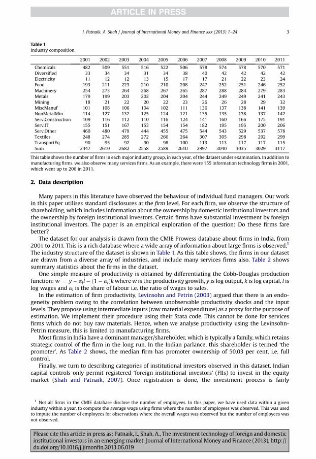
Table 1Industry composition.
2001 2002 2003 2004 2005 2006 2007 2008 2009 2010 2011
Chemicals 482 509 551 516 522 506 578 574 578 570 571Diversified 33 34 34 31 34 38 40 42 42 42 42Electricity 11 12 12 13 15 17 17 21 22 23 24Food 193 211 223 210 210 208 247 252 251 246 252Machinery 254 273 264 268 267 265 287 288 284 279 283Metals 179 199 203 202 204 204 244 249 249 241 243Mining 18 21 22 20 22 23 26 26 28 29 32MiscManuf 101 108 106 104 102 111 136 137 138 141 139NonMetalMin 114 127 132 125 124 121 135 135 138 137 142Serv.Construction 109 116 112 110 116 124 141 160 166 175 191Serv.IT 155 151 167 153 154 154 182 195 195 200 206Serv.Other 460 480 479 444 455 475 544 543 529 537 578Textiles 248 274 285 272 266 264 307 305 298 292 299TransportEq 90 95 92 90 98 100 113 113 117 117 115Sum 2447 2610 2682 2558 2589 2610 2997 3040 3035 3029 3117
This table shows the number of firms in eachmajor industry group, in each year, of the dataset under examination. In addition tomanufacturing firms, we also observemany services firms. As an example, there were 155 information technology firms in 2001,which went up to 206 in 2011.
I. Patnaik, A. Shah / Journal of International Money and Finance xxx (2013) 1–24 3
2. Data description
Many papers in this literature have observed the behaviour of individual fund managers. Our workin this paper utilises standard disclosures at the firm level. For each firm, we observe the structure ofshareholding, which includes information about the ownership by domestic institutional investors andthe ownership by foreign institutional investors. Certain firms have substantial investment by foreigninstitutional investors. The paper is an empirical exploration of the question: Do these firms farebetter?
The dataset for our analysis is drawn from the CMIE Prowess database about firms in India, from2001 to 2011. This is a rich database where a wide array of information about large firms is observed.1
The industry structure of the dataset is shown in Table 1. As this table shows, the firms in our datasetare drawn from a diverse array of industries, and include many services firms also. Table 2 showssummary statistics about the firms in the dataset.
One simple measure of productivity is obtained by differentiating the Cobb-Douglas productionfunction: _w ¼ _y� al
_l� ð1� alÞ _kwhere _w is the productivity growth, y is log output, k is log capital, l islog wages and al is the share of labour i.e. the ratio of wages to sales.
In the estimation of firm productivity, Levinsohn and Petrin (2003) argued that there is an endo-geneity problem owing to the correlation between unobservable productivity shocks and the inputlevels. They propose using intermediate inputs (rawmaterial expenditure) as a proxy for the purpose ofestimation. We implement their procedure using their Stata code. This cannot be done for servicesfirms which do not buy raw materials. Hence, when we analyse productivity using the Levinsohn-Petrin measure, this is limited to manufacturing firms.
Most firms in India have a dominantmanager/shareholder, which is typically a family, which retainsstrategic control of the firm in the long run. In the Indian parlance, this shareholder is termed ‘thepromoter’. As Table 2 shows, the median firm has promoter ownership of 50.03 per cent, i.e. fullcontrol.
Finally, we turn to describing categories of institutional investors observed in this dataset. Indiancapital controls only permit registered ‘foreign institutional investors’ (FIIs) to invest in the equitymarket (Shah and Patnaik, 2007). Once registration is done, the investment process is fairly
1 Not all firms in the CMIE database disclose the number of employees. In this paper, we have used data within a givenindustry within a year, to compute the average wage using firms where the number of employees was observed. This was usedto impute the number of employees for observations where the overall wages was observed but the number of employees wasnot observed.
Please cite this article in press as: Patnaik, I., Shah, A., The investment technology of foreign and domesticinstitutional investors in an emerging market, Journal of International Money and Finance (2013), http://dx.doi.org/10.1016/j.jimonfin.2013.06.019
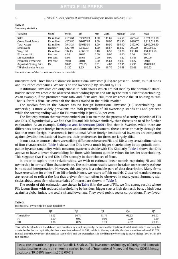
Table 2Summary statistics.
Variable Units Mean SD Min 25th Median 75th Max
Sales Rs. million 7153.61 63,329.24 1.00 141.65 645.50 2655.40 3,574,219.80Gross Fixed Assets Rs. million 4255.86 36,627.87 1.00 96.90 371.30 1486.70 2,212,519.70Total Assets Rs. million 7943.24 55,635.54 1.00 180.50 695.00 2892.00 2,849,003.50Employees Number 1227.04 5,342.23 1.00 35.57 183.07 790.70 159,999.57Wage bill Rs. million 337.15 2,669.62 0.10 6.50 30.20 130.10 134,173.50FII ownership Per cent 4.05 10.85 0.00 0.00 0.00 0.36 89.29DII ownership Per cent 9.60 15.66 0.00 0.00 1.22 13.48 100.00Promoter ownership Per cent 49.01 20.01 0.00 35.64 50.03 63.27 99.83Adjusted Closing Price Rs. 68.85 378.85 0.01 4.00 12.35 45.35 49,088.80TFP (Levinsohn Petrin) 21.25 8.25 1.00 18.70 20.68 22.49 186.55
Some features of the dataset are shown in the table.
I. Patnaik, A. Shah / Journal of International Money and Finance xxx (2013) 1–244
unconstrained. Three kinds of domestic institutional investors (DIIs) are present – banks, mutual fundsand insurance companies. We focus on the ownership by FIIs and by DIIs.
Institutional investors can only choose to hold shares which are not held by the dominant share-holder. Hence, we rescale the observed shareholding by FIIs and DIIs by the total outsider shareholding.As an example, if the promoter owns 60%, and if FIIs own 20%, then we rescale the FII holding to 50%.That is, for this firm, FIIs own half the shares traded in the public market.
The median firm in the dataset has no foreign institutional investor (FII) shareholding. DIIownership is more widely prevalent: the 75th percentile of DII ownership stands at 13.48 per centwhile the corresponding value for FII ownership is just 0.36 per cent.
The first exploration that we must embark on is to examine the process of security selection of FIIsand DIIs. If, hypothetically, we find that FIIs and DIIs behave similarly, then there is no need for furtherexploration. As an example, Dahlquist and Robertsson (2001) find that in Sweden, while there aredifferences between foreign investment and domestic investment, these derive primarily through thefact that most foreign investment is institutional. When foreign institutional investors are comparedagainst Swedish institutional investors, their preferences for firms are largely alike.
In our data, in contrast, there are striking differences between FIIs and DIIs along certain dimensionsof firm characteristics. Table 3 shows that DIIs have a much bigger shareholding in top quintile com-panies by asset tangibility, while no strong pattern is visible with FIIs. Similarly, Table 4 shows that DIIsappear to have a lower shareholding for firms with bottom quintile values for insider shareholding.This suggests that FIIs and DIIs differ strongly in their choices of firms.
In order to explore these relationships, we wish to estimate linear models explaining FII and DIIownership in terms of firm characteristics. The estimation results cannot be taken too seriously as thereis no causal interpretation. However, this analysis is a valuable part of data description. Many firmshave zero values for either FII or DII or both. Hence, we resort toTobit models. Clustered standard errorsare reported to reflect the fact that a given firm can often be observed in many years. Summary sta-tistics about some firm characteristics of interest are shown in Table 5.
The results of this estimation are shown in Table 6. In the case of FIIs, we find strong results whereFIIs favour firms with reduced shareholding by insiders, bigger size, a high domestic beta, a high betaagainst a global index, low total risk and lower age. They avoid public sector corporations. They favour
Table 3Institutional ownership by asset tangibility.
Q1 Q2 Q3 Q4 Q5
Tangibility 14.05 34.74 51.10 69.32 96.02FII 0.00 0.00 0.00 0.00 0.89DII 0.76 0.27 1.39 2.92 20.33
This table breaks down the dataset into quintiles by asset tangibility, defined as the fraction of total assets which are tangibleassets. In the bottom quintile, this has a median value of 14.05%, while in the top quintile, this has a median value of 96.02%.In each quintile, we report the median value of FII and DII ownership. The median DII ownership is much higher (20.33%) in thetop quintile.
Please cite this article in press as: Patnaik, I., Shah, A., The investment technology of foreign and domesticinstitutional investors in an emerging market, Journal of International Money and Finance (2013), http://dx.doi.org/10.1016/j.jimonfin.2013.06.019
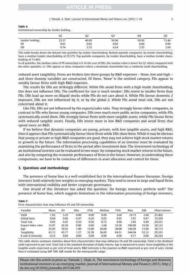
Table 4Institutional ownership by insider holding.
Q1 Q2 Q3 Q4 Q5
Insider holding 25.57 40.99 50.96 59.99 73.46FII 0.01 0.02 0.02 0.00 0.00DII 0.74 3.53 4.24 3.55 2.60
This table breaks down the dataset into quintiles by insider shareholding. Bottom quintile companies, by insider shareholding,have a median insider shareholding of 25.57%. Top quintile companies, by insider shareholding, have a median insider share-holding of 73.46%.In all quintiles, the median value of FII ownership is 0. In the case of DIIs, the median value is lower for Q1 when compared withthe other quintiles, i.e. DIIs appear to shun companies where a dominant shareholder has a relatively small shareholding.
I. Patnaik, A. Shah / Journal of International Money and Finance xxx (2013) 1–24 5
reduced asset tangibility. Firms are broken into three groups by R&D expenses – None, low and high –
and three dummy variables are constructed. Of these, ‘None’ is the omitted category. FIIs appear toweakly favour firms with high R&D expenses.
The results for DIIs are strikingly different. While FIIs avoid firms with a high inside shareholding,this does not influence DIIs. The coefficient for size is much weaker: DIIs invest in smaller firms thanFIIs. DIIs load up more on illiquid stocks while FIIs do not care about it. While FIIs favour domestic b
exposure, DIIs are not influenced by it, or by the global b. While FIIs avoid total risk, DIIs are notconcerned about it.
Like FIIs, DIIs are not influenced by the exports/sales ratio. They strongly favour older companies, incontrast to FIIs who favour young companies. DIIs own much more public sector companies, while FIIssystematically avoid them. DIIs strongly favour firms with more tangible assets, while FIIs favour firmswith reduced tangible assets. Finally, DIIs invest more in low R&D companies and avoid firms thatspend more on R&D.
If we believe that dynamic companies are young, private, with low tangible assets, and high R&D,then it appears that FIIs systematically favour these firmswhile DIIs shun them.While itmay be obviousthat young or private or high R&D companies are good, theymay not achieve high stockmarket returnsor growth in the future. The information processing capabilities of an investor must be evaluated byexamining the performance of firms in the period after investment date. The investment technology ofan institutional investor can be evaluated in twoways: by comparing stockmarket returns in the future,and also by comparing the economic performance of firms in the future. However, in undertaking thesecomparisons, we have to be conscious of differences in asset allocation and control for these.
3. Questions and methodology
The presence of home bias is a well established fact in the international finance literature: foreigninvestors hold relatively lowweights in emerging markets. They tend to invest in large and liquid firmswith international visibility and better corporate governance.
One strand of this literature has asked the question: Do foreign investors perform well? Thepresence of home bias, which suggests limitations in the information processing of foreign investors,
Table 5Firm characteristics that may influence FII and DII ownership.
Variable Mean SD Min 25th Median 75th Max IQR Observations
Yield 1.92 3.29 0.00 0.00 0.00 2.68 16.73 2.68 25,402Global beta 0.64 0.66 �6.47 0.29 0.63 0.95 7.61 0.67 15,250Total risk 0.85 0.47 0.26 0.56 0.72 0.96 2.86 0.40 20,251Export-Sales ratio 15.97 26.50 0.00 0.00 1.68 19.38 100.00 19.38 28,155Age 25.95 18.03 1.00 15.00 20.00 30.00 148.00 15.00 30,773Tangibility 63.13 43.77 1.27 32.38 56.69 84.51 244.94 52.12 29,101R and D intensity 0.23 0.89 0.00 0.00 0.00 0.00 6.77 0.00 28,243
This table shows summary statistics about firm characteristics that may influence FII and DII ownership. Yield is the dividendyield expressed in per cent. Total risk is the standard deviation of daily returns. Age is measured in years. Asset tangibility is thetangible assets expressed as per cent of total assets. R&D intensity is the expense on R&D expressed as per cent of sales. Globalbeta is estimated using S&P 500. IQR stands for the interquartile range.
Please cite this article in press as: Patnaik, I., Shah, A., The investment technology of foreign and domesticinstitutional investors in an emerging market, Journal of International Money and Finance (2013), http://dx.doi.org/10.1016/j.jimonfin.2013.06.019
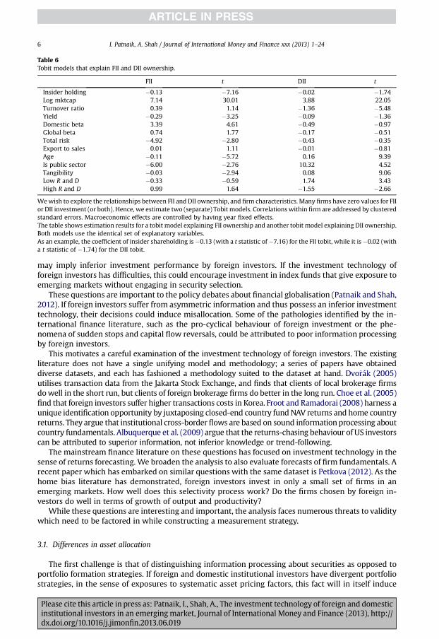
Table 6Tobit models that explain FII and DII ownership.
FII t DII t
Insider holding �0.13 �7.16 �0.02 �1.74Log mktcap 7.14 30.01 3.88 22.05Turnover ratio 0.39 1.14 �1.36 �5.48Yield �0.29 �3.25 �0.09 �1.36Domestic beta 3.39 4.61 �0.49 �0.97Global beta 0.74 1.77 �0.17 �0.51Total risk �4.92 �2.80 �0.43 �0.35Export to sales 0.01 1.11 �0.01 �0.81Age �0.11 �5.72 0.16 9.39Is public sector �6.00 �2.76 10.32 4.52Tangibility �0.03 �2.94 0.08 9.06Low R and D �0.33 �0.59 1.74 3.43High R and D 0.99 1.64 �1.55 �2.66
Wewish to explore the relationships between FII and DII ownership, and firm characteristics. Many firms have zero values for FIIor DII investment (or both). Hence, we estimate two (separate) Tobit models. Correlations within firm are addressed by clusteredstandard errors. Macroeconomic effects are controlled by having year fixed effects.The table shows estimation results for a tobit model explaining FII ownership and another tobit model explaining DII ownership.Both models use the identical set of explanatory variables.As an example, the coefficient of insider shareholding is�0.13 (with a t statistic of�7.16) for the FII tobit, while it is�0.02 (witha t statistic of �1.74) for the DII tobit.
I. Patnaik, A. Shah / Journal of International Money and Finance xxx (2013) 1–246
may imply inferior investment performance by foreign investors. If the investment technology offoreign investors has difficulties, this could encourage investment in index funds that give exposure toemerging markets without engaging in security selection.
These questions are important to the policy debates about financial globalisation (Patnaik and Shah,2012). If foreign investors suffer from asymmetric information and thus possess an inferior investmenttechnology, their decisions could induce misallocation. Some of the pathologies identified by the in-ternational finance literature, such as the pro-cyclical behaviour of foreign investment or the phe-nomena of sudden stops and capital flow reversals, could be attributed to poor information processingby foreign investors.
This motivates a careful examination of the investment technology of foreign investors. The existingliterature does not have a single unifying model and methodology; a series of papers have obtaineddiverse datasets, and each has fashioned a methodology suited to the dataset at hand. Dvo�rák (2005)utilises transaction data from the Jakarta Stock Exchange, and finds that clients of local brokerage firmsdowell in the short run, but clients of foreign brokerage firms do better in the long run. Choe et al. (2005)find that foreign investors suffer higher transactions costs in Korea. Froot and Ramadorai (2008) harness aunique identification opportunity by juxtaposing closed-end country fundNAV returns and home countryreturns. They argue that institutional cross-border flows are based on sound informationprocessing aboutcountry fundamentals. Albuquerque et al. (2009) argue that the returns-chasing behaviour of US investorscan be attributed to superior information, not inferior knowledge or trend-following.
The mainstream finance literature on these questions has focused on investment technology in thesense of returns forecasting. We broaden the analysis to also evaluate forecasts of firm fundamentals. Arecent paper which has embarked on similar questions with the same dataset is Petkova (2012). As thehome bias literature has demonstrated, foreign investors invest in only a small set of firms in anemerging markets. How well does this selectivity process work? Do the firms chosen by foreign in-vestors do well in terms of growth of output and productivity?
While these questions are interesting and important, the analysis faces numerous threats to validitywhich need to be factored in while constructing a measurement strategy.
3.1. Differences in asset allocation
The first challenge is that of distinguishing information processing about securities as opposed toportfolio formation strategies. If foreign and domestic institutional investors have divergent portfoliostrategies, in the sense of exposures to systematic asset pricing factors, this fact will in itself induce
Please cite this article in press as: Patnaik, I., Shah, A., The investment technology of foreign and domesticinstitutional investors in an emerging market, Journal of International Money and Finance (2013), http://dx.doi.org/10.1016/j.jimonfin.2013.06.019

I. Patnaik, A. Shah / Journal of International Money and Finance xxx (2013) 1–24 7
differences in portfolio performance. The investors who accept a greater exposure to risk factors, suchas investment in high beta, low size, and high B/P firms, will obtain superior expected returns. Thisdifference in returns should be interpreted as returns to asset allocation, and not related to informationprocessing or forecasting about emerging market firms.
Indeed, given that asset allocation is often largely determined by the investment mandate, to asubstantial extent, differences in asset allocation between foreign and domestic investors should notbe attributed to differences in the investment technology of foreign or domestic investors. As anexample, the investment mandate or chosen portfolio strategy of a foreign investor may requireinvestment in firms with a market capitalisation of above $1 billion. The security selection by thisinvestor must then be judged by comparisons against similar sized firms that were not chosen forinvestment.
These issues arise when evaluating other measures of firm performance also. High beta firms wouldtend to obtain high growth in a business cycle expansion. This would make it appear that an investorwith a high beta asset allocation possesses skills in security selection during a business cycle expansion.Before skills in security selection can be assessed, we have to control for differences in asset allocation.
Our first objective is thus to measure the asset allocation of domestic versus foreign investors. Theempirical asset pricing literature suggests that the Fama-French factors – size, B/P, and b – explain thebulk of the variation in portfolio performance. In our sensitivity analyses, we will also explore liquidityand momentum as potentially important asset pricing factors.
3.2. Differences in security selection
Our analysis of asset allocation (in Section 4) shows that foreign and domestic investors differ intheir choices on size, B/P and b.2 Traditional regression analysis would attempt to control for thesedifferences by running regressions where size, B/P and b are present as controls. However, suchanalysis suffers from two key problems: (a) The true relationship is likely to be nonlinear, resulting inmisspecification of conventional linear models and (b) When there is a lack of match balance, con-ventional linear models involve extrapolation, which is fraught with estimation risk.
Hence, we embark on a matching process, where each firm that was chosen by FIIs, but notDIIs (or by DIIs, but not FIIs) is matched against a partner that got neither FII nor DII invest-ment, where the chosen firm and the partner have similar values for size, B/P and b. If a highquality match is not obtained, the firm is deleted from the dataset. This ensures a high qualitydesign which gives us the ability to focus on security selection without being confounded bydifferences in asset allocation.
The questions of interest involve a complex interplay between selectivity effects and treatment ef-fects. Foreign investment is not a treatment in the sense of the literature on treatment effects. When aforeign investor buys shares on the secondary market, in some respects, the firm is unaffected. Further,foreign investors canflit in and out of ownership of the company. From this viewpoint, the phenomenonof interest is selection: Do foreign investors farewell in forecasting future stockmarket returns and thuspick winners? Do the firms that they choose experience high growth in output and productivity?
If the question under analysis were purely about treatment effects, then propensity score matchingwould have been appropriate. However, to the extent that the mechanism of selection is the phe-nomenon of interest, propensity score matching is inappropriate.3
2 Before we examine the security selection of foreign investors, two possibilities need to be ruled out. One possibility involvesforeign investors investing primarily in index funds. In this case, their returns would reflect exposure to systematic asset pricingfactors and the returns to security selection would be zero. Another possibility involves foreign and domestic investorschoosing alike. In this case, there would be no discernable difference between the security selection of foreign versus domesticinvestors. Our preliminary analysis in Section 2 has ruled out both these possibilities.
3 As an example, consider a firm characteristic X (e.g. export intensity) that is used by FIIs in identifying firms to invest in. If Xis present in the logit model used for propensity score matching, then the matched control will have similar values for X.However, this may obscure the phenomenon of interest. Focusing on high export companies may be a valuable part of theinvestment technology. If FIIs select firms for investment using export intensity, and if this yields high quality investments, thisphenomenon would not be captured by a comparison of treatment and control through propensity score matching.
Please cite this article in press as: Patnaik, I., Shah, A., The investment technology of foreign and domesticinstitutional investors in an emerging market, Journal of International Money and Finance (2013), http://dx.doi.org/10.1016/j.jimonfin.2013.06.019
I. Patnaik, A. Shah / Journal of International Money and Finance xxx (2013) 1–248
At the same time, there may also be an element of a casual impact of foreign investment upon thefirm. Foreign investors might get involved in corporate governance and thus improve the functioning ofthe firm. In a model of imperfect capital market integration such as Merton (1987), the entry of foreigninvestors into a firmmay be associated with enhanced stock prices, andmay enable improved access toequity and debt financing which may fuel growth of capital. If firms are financially constrained, thismight make it possible for them to take up good quality projects and thus obtain sharp improvementsin output and productivity.
In this paper, we recognise that both selection and treatment effects are present, and make noattempt to disentangle them. We focus on the reduced form question: Regardless of whether this isowing to selection or treatment effects, do the firms chosen for investment by foreign investment farewell in the future, in terms of growth in output, productivity and stock market returns?
3.3. The problems of comparing institutional investors against domestic individual investors
Most foreign investment in emerging markets is done by institutional investors, while mostdomestic investors in emerging markets are individuals. An extensive literature in financialintermediation has emphasised the unique decision problems of institutional investors. A morerecent household finance literature has identified unique features of the behaviour of individualinvestors.
In order to avoid comparisons between foreign institutional investors against domestic individualinvestors, we compare the behaviour of foreign institutional investors (FII) against domestic institu-tional investors (DII).
3.4. Identifying FII vs. DII
The simplest estimation strategy would involve running regressions explaining an outcome (e.g.output growth) from time t to time t þ k on ownership structure at time t. This would suffer from theproblem that many firms have both domestic and foreign institutional investment. The phenomena ofinterest are not identified for these firms.
Hence, we devise a quasi-experimental strategy by identifying two groups of firms: Thosewith highFII investment but not DII investment, and vice versa. The former set is the firms chosen by FIIs forinvestment but shunned byDIIs, and the latter is the firms chosen byDIIs for investment by shunned byFIIs. The comparison of performance by these firms would highlight the differences in informationprocessing (and potential treatment effects) by FIIs vs. DIIs.
3.5. Summary of methodology for measuring security selection
In summary, our strategy for measuring capabilities in security selection, after controlling for dif-ferences in asset allocation, works in three steps:
1. At each year, identify a ‘High FII’ set of firms, with high FII investment but lowDII investment, and a‘High DII’ set of firms, with high DII investment but low FII investment. A third set of firms ofinterest is ‘None’, where there is neither FII nor DII investment. Drop firms that have high FII andhigh DII investment.
2. For each firm in the High FII or High DII sets, identify a matched control from the set ’None’that has similar size, B/P and b. Reject chosen firms where a high quality match cannot beobtained.
3. This leaves us holding a dataset containing N firms with high FII investment (but not DII invest-ment) and another N firms with neither FII investment nor DII investment, where the two sets arematched by size, B/P and b. Observations across many years are pooled. This permits regressions ofthe form yi,tþk� yi,t¼ a0þ a1Dþ ei,twhere the growth in y is explained using the dummy variableDwhich denotes high FII investment. Clustered and heteroscedasticity-robust standard errors arereported.
Please cite this article in press as: Patnaik, I., Shah, A., The investment technology of foreign and domesticinstitutional investors in an emerging market, Journal of International Money and Finance (2013), http://dx.doi.org/10.1016/j.jimonfin.2013.06.019
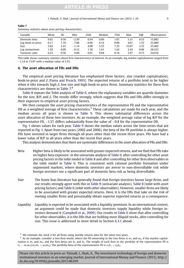
Table 7Summary statistics about asset pricing characteristics.
Variable Mean SD Min 25th Median 75th Max IQR Observations
Domestic beta 0.82 0.50 �2.50 0.54 0.80 1.07 5.31 0.53 15,882Log book-to-price 0.11 1.19 �7.06 �0.66 0.14 0.89 4.61 1.55 22,989Size 5.82 2.41 �1.14 4.00 5.55 7.35 15.07 3.35 25,402Log momentum 1.59 0.09 �0.12 1.56 1.61 1.62 2.43 0.06 28,523Turnover ratio 0.22 0.56 0.00 0.01 0.04 0.16 3.97 0.15 24,916
This table shows summary statistics about firm characteristics of interest. As an example, log market capitalisation ranged from�1.14 to 15.07 with a median value of 5.55.
I. Patnaik, A. Shah / Journal of International Money and Finance xxx (2013) 1–24 9
4. The asset allocation of FIIs and DIIs
The empirical asset pricing literature has emphasised three factors: size (market capitalisation),book-to-price and b (Fama and French, 1993). The expected returns of a portfolio tend to be higherwhen it tilts towards high b, low size and high book-to-price firms. Summary statistics for these firmcharacteristics are shown in Table 7.4
Table 8 repeats the Tobit analysis of Table 6, where the explanatory variables are quartile dummiesfor the size, B/P, and b. The results differ strongly, which suggests that FIIs and DIIs differ strongly intheir exposure to empirical asset pricing factors.
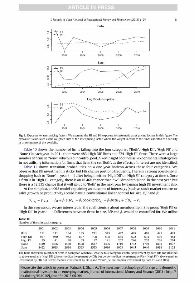
We then compute the asset pricing characteristics of the representative FII and the representativeDII as a weighted average of firm characteristics.5 These calculations are made for each year, and themedian across all years is shown in Table 9. This shows substantial differences across theasset allocation of these two investors. As an example, the weighted average value of log B/P for therepresentative FII, �1.37, differs substantially from the value of �0.8 for the representative DII.
Fig. 1 shows values for each year. Table 9 shows the median values across the time-series that arereported in Fig. 1. Apart from two years (2002 and 2006), the beta of the FII portfolio is always higher.FIIs have invested in larger firms through all years other than the recent three years. FIIs have had alower value of B/P in all years other than the recent four years.
This analysis demonstrates that there are systematic differences in the asset allocation of FIIs and DIIs:
Beta Higher beta is likely to be associatedwith greater expected returns, andwe find that FIIs takeon higher beta exposure: in the univariate analysis of Table 9, after controlling for other assetpricing factors in the tobit model in Table 8 and after controlling for other firm observables inthe tobit model in Table 6. This is consistent with rational portfolio formation undersegmented markets, where domestic investors are averse to non-diversifiable risk whileforeign investors see a significant part of domestic beta risk as being diversifiable.
Size The home bias literature has generally found that foreign investors favour large firms, andour results strongly agree with this in Table 9 (univariate analysis), Table 8 (tobit with assetpricing factors) and Table 6 (tobit with other observables). However, smaller firms are likelyto be associated with greater expected returns. Here, it is the DIIs that take on the risk ofowning smaller firms and presumably obtain superior expected returns as a consequence.
Liquidity Liquidity is expected to be associated with a liquidity premium. In an international context,an argument could be made that domestic investors supply liquidity while foreign in-vestors demand it (Campbell et al., 2009). Our results in Table 6 show that after controllingfor other observables, it is the DIIs that are holding more illiquid stocks, after controlling forsize. This issue is addressed in more detail in Section 6.3.1 ahead.
4 We estimate the stock b for all firms using weekly returns data for the latest two years.5 As an example, consider a two-firm world, where the FII ownership in the two firms is w1 and w2, if the market capital-
isation is m1 and m2, and the firm betas are b1 and b2. The weight of each firm in the portfolio of the representative FII isx1 ¼ w1m1/(w1m1 þ w2m2). The portfolio beta of the representative FII is x1b1 þ x2b2.
Please cite this article in press as: Patnaik, I., Shah, A., The investment technology of foreign and domesticinstitutional investors in an emerging market, Journal of International Money and Finance (2013), http://dx.doi.org/10.1016/j.jimonfin.2013.06.019
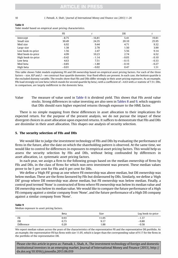
Table 8Tobit model based on empirical asset pricing characteristics.
FII t DII t
Intercept �8.75 �16.81 5.41 19.81Small size 30.49 24.35 20.10 25.95Med size 6.92 9.44 4.71 9.32Large size 1.38 2.78 1.50 3.99Low book-to-price 1.56 2.47 5.56 9.14Med book-to-price 4.99 10.23 2.74 6.52High book-to-price �0.42 �1.14 �0.03 �0.10Low beta 4.63 7.51 �0.15 �0.33Med beta �0.85 �1.80 �0.10 �0.27High beta �0.01 �0.02 0.47 1.51
This table shows Tobit models explaining FII and DII ownership based on empirical asset pricing factors. For each of the threefactors – size, B/P and b –we construct four quartile dummies. Year fixed effects are present. In each case, the bottom quartile isthe excluded dummy variable. The results show that FIIs and DIIs differ strongly in their asset pricing exposures. As an example,FIIs load strongly on Low beta (which stands for second quartile by beta), with a coefficient ofþ4.63 with a t statistic of 7.51. DIIs,in comparison, are largely indifferent to the domestic beta.
I. Patnaik, A. Shah / Journal of International Money and Finance xxx (2013) 1–2410
Value The measure of value used in Table 6 is dividend yield. This shows that FIIs avoid valuestocks. Strong differences in value investing are also seen in Tables 8 and 9, which suggeststhat DIIs should earn higher expected returns through exposure to the HML factor.
There is no simple mapping from these differences in asset allocation to their implications forexpected return. For the purpose of the present analysis, we do not pursue the impact of thesedivergent choices in asset allocation upon expected returns. It suffices to demonstrate that FIIs and DIIsare dissimilar in their asset allocation. This shapes our analysis of security selection.
5. The security selection of FIIs and DIIs
Wewould like to judge the investment technology of FIIs and DIIs by evaluating the performance offirms in the future, after the date onwhich the shareholding pattern is observed. At the same time, wewould like to control for differences in exposures to empirical asset pricing factors. This would help usassess the security selection by FIIs and DIIs, without being confounded by differences inasset allocation, i.e. systematic asset pricing factors.
In each year, we assign a firm to the following groups based on the median ownership of firms byFIIs and DIIs, in the class of firms for which non-zero investment was present. These median valuesprove to be 5 per cent for FIIs and 6 per cent for DIIs.
We define a ‘High FII’ group as one where FII ownership was above median, but DII ownership wasbelowmedian. These are the firms favoured by FIIs but disfavoured by DIIs. Similarly, we define a ‘HighDII’ group where DII ownership was above median, but FII ownership was below median. Finally, acontrol pool termed ‘None’ is constructed of firmswhere FII ownership was below its median value andDII ownership was below its median value. Wewould like to compare the future performance of a HighFII company against a similar company from ‘None’, and the future performance of a High DII companyagainst a similar company from ‘None’.
Table 9Median exposure to asset pricing factors.
Beta Size Log book-to-price
FII 0.93 11.05 �1.37DII 0.73 9.17 �0.80Difference 0.20 1.88 �0.58
We report median values across the years of the characteristics of the representative FII and the representative DII portfolio. Asan example, the representative FII has firms with size 11.05, which is larger than the corresponding value of 9.17 for the firms inthe portfolio of the representative DII.
Please cite this article in press as: Patnaik, I., Shah, A., The investment technology of foreign and domesticinstitutional investors in an emerging market, Journal of International Money and Finance (2013), http://dx.doi.org/10.1016/j.jimonfin.2013.06.019
2002 2004 2006 2008 2010
0.51.01.5
Beta
FIIDII
2002 2004 2006 2008 2010
9.010.0
11.5
Size
FIIDII
2002 2004 2006 2008 2010
−2.5
−1.5
−0.5
Log Book−to−price
FIIDII
Fig. 1. Exposure to asset pricing factors. We examine the FII and DII exposure to systematic asset pricing factors in this figure. Theexposure is calculated as the weighted sum of the asset pricing factor, where the weight is equal to the funds allocated to a securityas a percentage of the portfolio.
I. Patnaik, A. Shah / Journal of International Money and Finance xxx (2013) 1–24 11
Table 10 shows the number of firms falling into the four categories (‘Both’, ‘High DII’, ‘High FII’ and‘None’) in each year. In 2011, there were 483 ‘High DII’ firms and 274 ‘High FII’ firms. There were a largenumber of firms in ‘None’, which is our control pool. A key insight of our quasi-experimental strategy liesin not utilising information for firms that lie in the set ‘Both’, as the effects of interest are not identified.
Table 11 shows transition probabilities on a one year horizon across these four categories. Weobserve that DII investment is sticky, but FIIs change portfolio frequently. There is a strong possibility ofdropping back to ‘None’ in year tþ 1 after being in either ‘High DII’ or ‘High FII’ category at time t. Oncea firm is in ‘High FII’ category, there is an 18.46% chance that it will drop into ‘None’ in the next year, butthere is a 12.33% chance that it will go up to ‘Both’ in the next year by gaining high DII investment also.
At the simplest, an OLS model explaining an outcome of interest yit (such as stock market returns orsales growth or productivity) could have a conventional linear control for size, B/P and b:
yi;tþj � yi;t�k ¼ b0 þ b1sizei;t þ b2book=pricei;t þ b3betai;t þ g0Di;t þ eit
In this regression, we are interested in the coefficients g aboutmembership in the group ‘High FII’ or‘High DII’ in year t � 1. Differences between firms in size, B/P and b. would be controlled for. We utilise
Table 10Number of firms in each category.
2001 2002 2003 2004 2005 2006 2007 2008 2009 2010 2011
Both 181 141 134 185 241 375 442 495 416 421 428High DII 927 980 962 807 708 598 635 572 593 539 483High FII 35 41 38 63 97 141 207 246 262 236 274None 1319 1466 1560 1508 1547 1496 1719 1732 1769 1838 1937Sum 2462 2628 2694 2563 2593 2610 3003 3045 3040 3034 3122
The table shows the number of firms in each year, which fall into the four categories ‘Both’ (investment by both FIIs and DIIs thatis above-median), ‘High DII’ (above-median investment by DIIs but below-median investment by FIIs), ‘High FII’ (above-medianinvestment by FIIs but below-median investment by DIIs) and ‘None’ (below-median investment by both FIIs and DIIs).
Please cite this article in press as: Patnaik, I., Shah, A., The investment technology of foreign and domesticinstitutional investors in an emerging market, Journal of International Money and Finance (2013), http://dx.doi.org/10.1016/j.jimonfin.2013.06.019
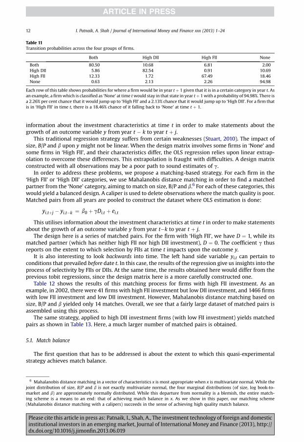
Table 11Transition probabilities across the four groups of firms.
Both High DII High FII None
Both 80.50 10.68 6.81 2.00High DII 5.86 82.54 0.91 10.69High FII 12.33 1.72 67.49 18.46None 0.63 2.13 2.26 94.98
Each row of this table shows probabilities for where a firmwould be in year tþ 1 given that it is in a certain category in year t. Asan example, a firmwhich is classified as ‘None’ at time twould stay in that state in year tþ 1with a probability of 94.98%. There isa 2.26% per cent chance that it would jump up to ‘High FII’ and a 2.13% chance that it would jump up to ‘High DII’. For a firm thatis in ‘High FII’ in time t, there is a 18.46% chance of it falling back to ‘None’ at time t þ 1.
I. Patnaik, A. Shah / Journal of International Money and Finance xxx (2013) 1–2412
information about the investment characteristics at time t in order to make statements about thegrowth of an outcome variable y from year t � k to year t þ j.
This traditional regression strategy suffers from certain weaknesses (Stuart, 2010). The impact ofsize, B/P and b upon y might not be linear. When the design matrix involves some firms in ‘None’ andsome firms in ‘High FII’, and their characteristics differ, the OLS regression relies upon linear extrap-olation to overcome these differences. This extrapolation is fraught with difficulties. A design matrixconstructed with all observations may be a poor path to sound estimates of g.
In order to address these problems, we propose a matching-based strategy. For each firm in the‘High FII’ or ‘High DII’ categories, we use Mahalanobis distance matching in order to find a matchedpartner from the ‘None’ category, aiming to match on size, B/P and b.6 For each of these categories, thiswould yield a balanced design. A caliper is used to delete observations where the match quality is poor.Matched pairs from all years are pooled to construct the dataset where OLS estimation is done:
yi;tþj � yi;t�k ¼ b0 þ gDi;t þ ei;t
This utilises information about the investment characteristics at time t in order to make statementsabout the growth of an outcome variable y from year t�k to year t þ j.
The design here is a series of matched pairs. For the firm with ‘High FII’, we have D ¼ 1, while itsmatched partner (which has neither high FII nor high DII investment), D ¼ 0. The coefficient g thusreports on the extent to which selection by FIIs at time t impacts upon the outcome y.
It is also interesting to look backwards into time. The left hand side variable yi,t can pertain toconditions that prevailed before date t. In this case, the results of the regression give us insights into theprocess of selectivity by FIIs or DIIs. At the same time, the results obtained here would differ from theprevious tobit regressions, since the design matrix here is a more carefully constructed one.
Table 12 shows the results of this matching process for firms with high FII investment. As anexample, in 2002, there were 41 firms with high FII investment but low DII investment, and 1466 firmswith low FII investment and low DII investment. However, Mahalanobis distance matching based onsize, B/P and b yielded only 14 matches. Overall, we see that a fairly large dataset of matched pairs isassembled using this process.
The same strategy, applied to high DII investment firms (with low FII investment) yields matchedpairs as shown in Table 13. Here, a much larger number of matched pairs is obtained.
5.1. Match balance
The first question that has to be addressed is about the extent to which this quasi-experimentalstrategy achieves match balance.
6 Mahalanobis distance matching in a vector of characteristics x is most appropriate when x is multivariate normal. While thejoint distribution of size, B/P and b is not exactly multivariate normal, the four marginal distributions (of size, log book-to-market and b) are approximately normally distributed. While this departure from normality is a blemish, the entire match-ing scheme is a means to an end: that of achieving match balance in x. As we show in this paper, our matching scheme(Mahalanobis distance matching with a calipers) succeeds in the sense of achieving high quality match balance.
Please cite this article in press as: Patnaik, I., Shah, A., The investment technology of foreign and domesticinstitutional investors in an emerging market, Journal of International Money and Finance (2013), http://dx.doi.org/10.1016/j.jimonfin.2013.06.019
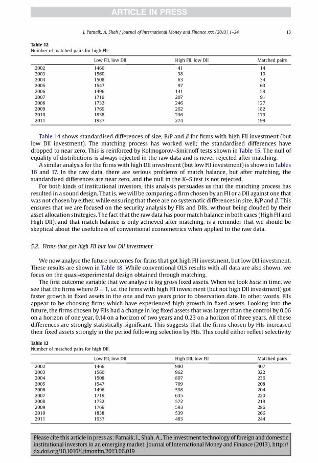
Table 12Number of matched pairs for high FII.
Low FII, low DII High FII, low DII Matched pairs
2002 1466 41 142003 1560 38 102004 1508 63 342005 1547 97 632006 1496 141 592007 1719 207 912008 1732 246 1272009 1769 262 1822010 1838 236 1792011 1937 274 199
I. Patnaik, A. Shah / Journal of International Money and Finance xxx (2013) 1–24 13
Table 14 shows standardised differences of size, B/P and b for firms with high FII investment (butlow DII investment). The matching process has worked well; the standardised differences havedropped to near zero. This is reinforced by Kolmogorov–Smirnoff tests shown in Table 15. The null ofequality of distributions is always rejected in the raw data and is never rejected after matching.
A similar analysis for the firms with high DII investment (but low FII investment) is shown in Tables16 and 17. In the raw data, there are serious problems of match balance, but after matching, thestandardised differences are near zero, and the null in the K–S test is not rejected.
For both kinds of institutional investors, this analysis persuades us that the matching process hasresulted in a sound design. That is, wewill be comparing a firm chosen by an FII or a DII against one thatwas not chosen by either, while ensuring that there are no systematic differences in size, B/P and b. Thisensures that we are focused on the security analysis by FIIs and DIIs, without being clouded by theirasset allocation strategies. The fact that the raw data has poormatch balance in both cases (High FII andHigh DII), and that match balance is only achieved after matching, is a reminder that we should beskeptical about the usefulness of conventional econometrics when applied to the raw data.
5.2. Firms that got high FII but low DII investment
We now analyse the future outcomes for firms that got high FII investment, but low DII investment.These results are shown in Table 18. While conventional OLS results with all data are also shown, wefocus on the quasi-experimental design obtained through matching.
The first outcome variable that we analyse is log gross fixed assets. When we look back in time, wesee that the firms where D ¼ 1, i.e. the firms with high FII investment (but not high DII investment) gotfaster growth in fixed assets in the one and two years prior to observation date. In other words, FIIsappear to be choosing firms which have experienced high growth in fixed assets. Looking into thefuture, the firms chosen by FIIs had a change in log fixed assets that was larger than the control by 0.06on a horizon of one year, 0.14 on a horizon of two years and 0.23 on a horizon of three years. All thesedifferences are strongly statistically significant. This suggests that the firms chosen by FIIs increasedtheir fixed assets strongly in the period following selection by FIIs. This could either reflect selectivity
Table 13Number of matched pairs for high DII.
Low FII, low DII High DII, low FII Matched pairs
2002 1466 980 4072003 1560 962 3222004 1508 807 2362005 1547 709 2082006 1496 598 2042007 1719 635 2202008 1732 572 2192009 1769 593 2862010 1838 539 2662011 1937 483 244
Please cite this article in press as: Patnaik, I., Shah, A., The investment technology of foreign and domesticinstitutional investors in an emerging market, Journal of International Money and Finance (2013), http://dx.doi.org/10.1016/j.jimonfin.2013.06.019
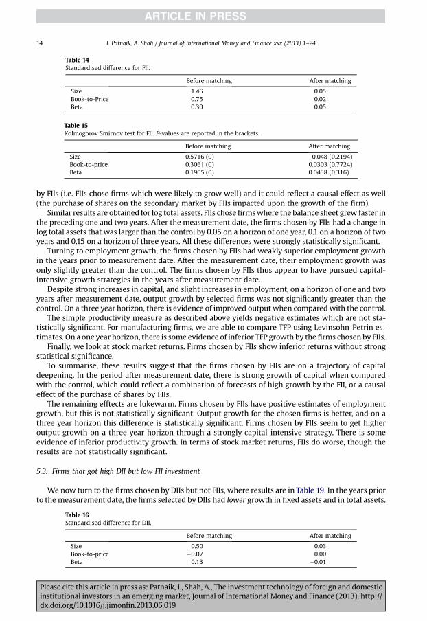
Table 14Standardised difference for FII.
Before matching After matching
Size 1.46 0.05Book-to-Price �0.75 �0.02Beta 0.30 0.05
Table 15Kolmogorov Smirnov test for FII. P-values are reported in the brackets.
Before matching After matching
Size 0.5716 (0) 0.048 (0.2194)Book-to-price 0.3061 (0) 0.0303 (0.7724)Beta 0.1905 (0) 0.0438 (0.316)
I. Patnaik, A. Shah / Journal of International Money and Finance xxx (2013) 1–2414
by FIIs (i.e. FIIs chose firms which were likely to grow well) and it could reflect a causal effect as well(the purchase of shares on the secondary market by FIIs impacted upon the growth of the firm).
Similar results are obtained for log total assets. FIIs chosefirmswhere the balance sheet grew faster inthe preceding one and two years. After the measurement date, the firms chosen by FIIs had a change inlog total assets that was larger than the control by 0.05 on a horizon of one year, 0.1 on a horizon of twoyears and 0.15 on a horizon of three years. All these differences were strongly statistically significant.
Turning to employment growth, the firms chosen by FIIs had weakly superior employment growthin the years prior to measurement date. After the measurement date, their employment growth wasonly slightly greater than the control. The firms chosen by FIIs thus appear to have pursued capital-intensive growth strategies in the years after measurement date.
Despite strong increases in capital, and slight increases in employment, on a horizon of one and twoyears after measurement date, output growth by selected firms was not significantly greater than thecontrol. On a three year horizon, there is evidence of improved output when comparedwith the control.
The simple productivity measure as described above yields negative estimates which are not sta-tistically significant. For manufacturing firms, we are able to compare TFP using Levinsohn-Petrin es-timates. On a one year horizon, there is some evidence of inferior TFP growth by thefirms chosen by FIIs.
Finally, we look at stock market returns. Firms chosen by FIIs show inferior returns without strongstatistical significance.
To summarise, these results suggest that the firms chosen by FIIs are on a trajectory of capitaldeepening. In the period after measurement date, there is strong growth of capital when comparedwith the control, which could reflect a combination of forecasts of high growth by the FII, or a causaleffect of the purchase of shares by FIIs.
The remaining efftects are lukewarm. Firms chosen by FIIs have positive estimates of employmentgrowth, but this is not statistically significant. Output growth for the chosen firms is better, and on athree year horizon this difference is statistically significant. Firms chosen by FIIs seem to get higheroutput growth on a three year horizon through a strongly capital-intensive strategy. There is someevidence of inferior productivity growth. In terms of stock market returns, FIIs do worse, though theresults are not statistically significant.
5.3. Firms that got high DII but low FII investment
We now turn to the firms chosen by DIIs but not FIIs, where results are in Table 19. In the years priorto the measurement date, the firms selected by DIIs had lower growth in fixed assets and in total assets.
Table 16Standardised difference for DII.
Before matching After matching
Size 0.50 0.03Book-to-price �0.07 0.00Beta 0.13 �0.01
Please cite this article in press as: Patnaik, I., Shah, A., The investment technology of foreign and domesticinstitutional investors in an emerging market, Journal of International Money and Finance (2013), http://dx.doi.org/10.1016/j.jimonfin.2013.06.019
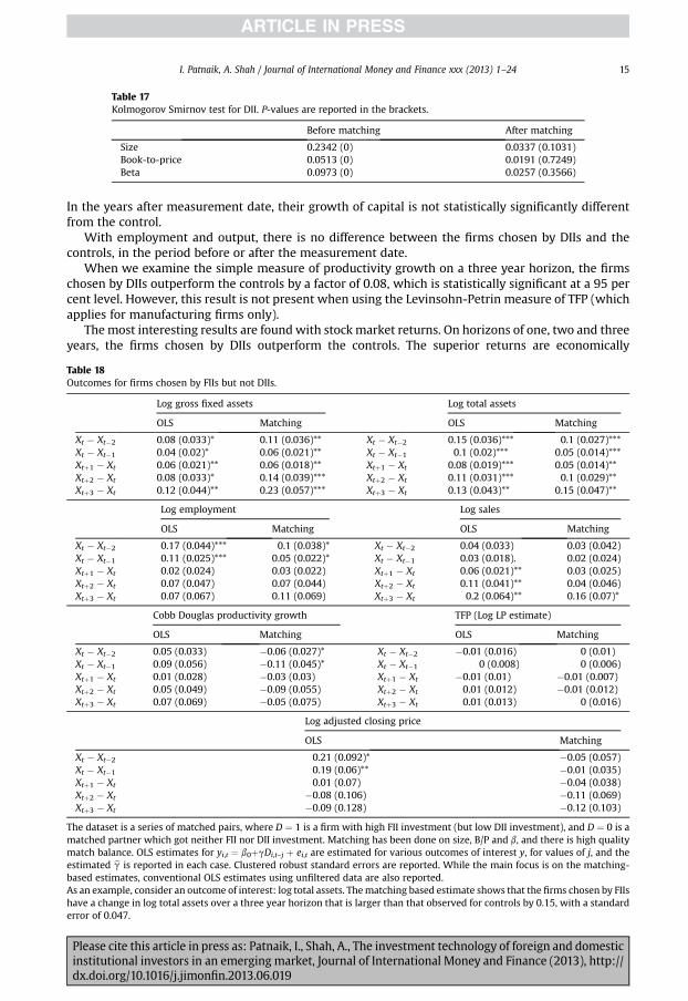
Table 17Kolmogorov Smirnov test for DII. P-values are reported in the brackets.
Before matching After matching
Size 0.2342 (0) 0.0337 (0.1031)Book-to-price 0.0513 (0) 0.0191 (0.7249)Beta 0.0973 (0) 0.0257 (0.3566)
I. Patnaik, A. Shah / Journal of International Money and Finance xxx (2013) 1–24 15
In the years after measurement date, their growth of capital is not statistically significantly differentfrom the control.
With employment and output, there is no difference between the firms chosen by DIIs and thecontrols, in the period before or after the measurement date.
When we examine the simple measure of productivity growth on a three year horizon, the firmschosen by DIIs outperform the controls by a factor of 0.08, which is statistically significant at a 95 percent level. However, this result is not present when using the Levinsohn-Petrin measure of TFP (whichapplies for manufacturing firms only).
The most interesting results are found with stockmarket returns. On horizons of one, two and threeyears, the firms chosen by DIIs outperform the controls. The superior returns are economically
Table 18Outcomes for firms chosen by FIIs but not DIIs.
Log gross fixed assets Log total assets
OLS Matching OLS Matching
Xt � Xt�2 0.08 (0.033)* 0.11 (0.036)** Xt � Xt�2 0.15 (0.036)*** 0.1 (0.027)***Xt � Xt�1 0.04 (0.02)* 0.06 (0.021)** Xt � Xt�1 0.1 (0.02)*** 0.05 (0.014)***Xtþ1 � Xt 0.06 (0.021)** 0.06 (0.018)** Xtþ1 � Xt 0.08 (0.019)*** 0.05 (0.014)**Xtþ2 � Xt 0.08 (0.033)* 0.14 (0.039)*** Xtþ2 � Xt 0.11 (0.031)*** 0.1 (0.029)**Xtþ3 � Xt 0.12 (0.044)** 0.23 (0.057)*** Xtþ3 � Xt 0.13 (0.043)** 0.15 (0.047)**
Log employment Log sales
OLS Matching OLS Matching
Xt � Xt�2 0.17 (0.044)*** 0.1 (0.038)* Xt � Xt�2 0.04 (0.033) 0.03 (0.042)Xt � Xt�1 0.11 (0.025)*** 0.05 (0.022)* Xt � Xt�1 0.03 (0.018). 0.02 (0.024)Xtþ1 � Xt 0.02 (0.024) 0.03 (0.022) Xtþ1 � Xt 0.06 (0.021)** 0.03 (0.025)Xtþ2 � Xt 0.07 (0.047) 0.07 (0.044) Xtþ2 � Xt 0.11 (0.041)** 0.04 (0.046)Xtþ3 � Xt 0.07 (0.067) 0.11 (0.069) Xtþ3 � Xt 0.2 (0.064)** 0.16 (0.07)*
Cobb Douglas productivity growth TFP (Log LP estimate)
OLS Matching OLS Matching
Xt � Xt�2 0.05 (0.033) �0.06 (0.027)* Xt � Xt�2 �0.01 (0.016) 0 (0.01)Xt � Xt�1 0.09 (0.056) �0.11 (0.045)* Xt � Xt�1 0 (0.008) 0 (0.006)Xtþ1 � Xt 0.01 (0.028) �0.03 (0.03) Xtþ1 � Xt �0.01 (0.01) �0.01 (0.007)Xtþ2 � Xt 0.05 (0.049) �0.09 (0.055) Xtþ2 � Xt 0.01 (0.012) �0.01 (0.012)Xtþ3 � Xt 0.07 (0.069) �0.05 (0.075) Xtþ3 � Xt 0.01 (0.013) 0 (0.016)
Log adjusted closing price
OLS Matching
Xt � Xt�2 0.21 (0.092)* �0.05 (0.057)Xt � Xt�1 0.19 (0.06)** �0.01 (0.035)Xtþ1 � Xt 0.01 (0.07) �0.04 (0.038)Xtþ2 � Xt �0.08 (0.106) �0.11 (0.069)Xtþ3 � Xt �0.09 (0.128) �0.12 (0.103)
The dataset is a series of matched pairs, where D ¼ 1 is a firm with high FII investment (but low DII investment), and D ¼ 0 is amatched partner which got neither FII nor DII investment. Matching has been done on size, B/P and b, and there is high qualitymatch balance. OLS estimates for yi,t ¼ b0þgDi,t–j þ ei,t are estimated for various outcomes of interest y, for values of j, and theestimated bg is reported in each case. Clustered robust standard errors are reported. While the main focus is on the matching-based estimates, conventional OLS estimates using unfiltered data are also reported.As an example, consider an outcome of interest: log total assets. Thematching based estimate shows that the firms chosen by FIIshave a change in log total assets over a three year horizon that is larger than that observed for controls by 0.15, with a standarderror of 0.047.
Please cite this article in press as: Patnaik, I., Shah, A., The investment technology of foreign and domesticinstitutional investors in an emerging market, Journal of International Money and Finance (2013), http://dx.doi.org/10.1016/j.jimonfin.2013.06.019

I. Patnaik, A. Shah / Journal of International Money and Finance xxx (2013) 1–2416
significant: 7 per cent on a one year horizon (with a standard error of 2.3 percentage points), 12 percent on a two year horizon (with a standard error of 3.8 percentage points) and 18 per cent on a threeyear horizon (with a standard error of 5.7 percentage points).
The firms chosen by DIIs yield superior stock market returns when compared with controls, whilethe firms chosen by FIIs do not. This suggests that DIIs possess a valuable investment technology whileFIIs do not. While the firms that FIIs invest in experience exuberant growth, there are concerns aboutproductivity, and superior stock market returns are not obtained. In contrast, DIIs appear to getinvolved in firms that are not on a high growth trajectory. However, there is some evidence of gains inproductivity and strong evidence about superior stock market returns.
6. Sensitivity analyses
We assess the robustness of these results by undertaking three alternative estimations.
1. Size weights2. More extreme definitions of FII and DII3. Alternative choices of asset pricing factors
Table 19Outcomes for firms chosen by DIIs but not FIIs.
Log gross fixed assets Log total assets
OLS Matching OLS Matching
Xt � Xt�2 �0.1 (0.02)*** �0.05 (0.02)* Xt � Xt�2 �0.1 (0.018)*** �0.06 (0.015)***Xt � Xt�1 �0.05 (0.011)*** �0.02 (0.01) Xt � Xt�1 �0.04 (0.01)*** �0.01 (0.008)Xtþ1 � Xt �0.03 (0.01)* �0.01 (0.012) Xtþ1 � Xt �0.01 (0.01) �0.01 (0.009)Xtþ2 � Xt �0.05 (0.02)** �0.02 (0.023) Xtþ2 � Xt �0.02 (0.018) �0.02 (0.017)Xtþ3 � Xt �0.05 (0.031) �0.04 (0.033) Xtþ3�Xt �0.01 (0.026) �0.02 (0.025)
Log employment Log sales
OLS Matching OLS Matching
Xt � Xt�2 �0.06 (0.024)** �0.02 (0.021) Xt � Xt�2 �0.05 (0.021)* 0 (0.025)Xt � Xt�1 �0.03 (0.013)* 0 (0.013) Xt � Xt�1 �0.02 (0.012) 0.01 (0.015)Xtþ1 � Xt �0.03 (0.015) 0.01 (0.013) Xtþ1 � Xt 0.01 (0.015) 0 (0.017)Xtþ2 � Xt �0.03 (0.026) �0.02 (0.024) Xtþ2 � Xt 0.03 (0.028) 0.01 (0.032)Xtþ3 � Xt �0.01 (0.036) �0.04 (0.035) Xtþ3 � Xt 0.05 (0.04) 0.06 (0.044)
Cobb Douglas productivity growth TFP (Log LP estimate)
OLS Matching OLS Matching
Xt � Xt�2 0.02 (0.018) 0.02 (0.016) Xt � Xt�2 0 (0.007) 0 (0.006)Xt � Xt�1 0.05 (0.03) 0.04 (0.026) Xt � Xt�1 0 (0.005) 0 (0.004)Xtþ1 � Xt 0.03 (0.018) 0 (0.017) Xtþ1 � Xt 0.01 (0.005) 0 (0.004)Xtþ2 � Xt 0.09 (0.031)** 0.03 (0.031) Xtþ2 � Xt 0.02 (0.006)* 0.01 (0.006)Xtþ3 � Xt 0.13 (0.043)** 0.08 (0.042)* Xtþ3 � Xt 0.01 (0.008) 0.01 (0.01)
Log adjusted closing price
OLS Matching
Xt � Xt�2 0.05 (0.052) 0.03 (0.035)Xt � Xt�1 0.06 (0.03) 0.04 (0.021)Xtþ1 � Xt 0.17 (0.034)*** 0.07 (0.023)**Xtþ2 � Xt 0.25 (0.053)*** 0.12 (0.038)**Xtþ3 � Xt 0.26 (0.066)*** 0.18 (0.057)**
The dataset is a series of matched pairs, where D ¼ 1 is a firm with high DII investment (but low FII investment), and D ¼ 0 is amatched partner which got neither FII nor DII investment. Matching has been done on size, B/P and b, and there is high qualitymatch balance. OLS estimates for yi,t ¼ b0 þ gDi,t–j þ ei,t are estimated for various outcomes of interest y, for values of j, and theestimated g
ˆis reported in each case. Clustered robust standard errors are reported. While the main focus is on the matching-
based estimates, conventional OLS estimates using unfiltered data are also reported.As an example, consider an outcome of interest: log total assets. The matching based estimate shows that the firms chosen byDIIs have a change in log total assets two years prior to measurement date that is larger than that observed for controls by�0.06,with a standard error of 0.015.
Please cite this article in press as: Patnaik, I., Shah, A., The investment technology of foreign and domesticinstitutional investors in an emerging market, Journal of International Money and Finance (2013), http://dx.doi.org/10.1016/j.jimonfin.2013.06.019
I. Patnaik, A. Shah / Journal of International Money and Finance xxx (2013) 1–24 17
6.1. Size weights
Themain results shown in the paper treated all firms as equal. This may give undue importance to alarge number of small firms. Hence, we undertake the same analysis with size weights. Size is definedas the average of firm sales and firm total assets.
The results for firms with high FII investment (but not high DII investment) are presented in Table22 in the appendix. As with the main results, firms chosen by FIIs (but not DIIs) experience rapidgrowth of capital, prior to the measurement year and after it. While there is improvement inemployment growth on a horizon of one year, this does not take place over two and three year hori-zons. However, this is associated with inferior productivity growth. The coefficients at all horizons arenegative but not statistically significant. There is no evidence of superior stock market returns.
Size-weighted results for firms with high DII investment (but not high FII investment) are presentedin Table 23 in the appendix. These are also qualitatively similar to the main results. These firms haveexperienced declining total assets for the years prior to measurement date and both one and threeyears after measurement date. Employment and output growth appear to be no different from thecontrol prior to measurement date, though they are significantly lesser than the control firm over ahorizon of two and three years. However, there is strong evidence of superior productivity growth.There is also strong evidence of superior stock market returns by 15% on a one year horizon and 21% ona two year horizon. This suggests that DIIs have an impressive investment technology while FIIs do not.
6.2. More extreme definitions for FII and DII dummies
Themain results of the paper were based onmedian values for FII and DII investment of five and sixper cent respectively. That is, a “High FII investment” firm was defined as one with more than 5%ownership of non-promoter shares by FIIs.
We redo the calculations using a more extreme definition. We define a High FII group as one whereFII ownership was above 12.5% (i.e. 66th percentile of the distribution of FII investment), and DIIownership was below 1.35% (i.e. 33rd percentile of the distribution of DII investment). Similarly, wedefine a High DII group where DII ownership was above 18.6%, but FII ownership was below 3.23%. Thecontrol group is constructed of firms where neither FII nor DII ownership was above their 33rdpercentile values.
Table 24, in the appendix, shows the results for firms with high FII investment (but low DII in-vestment). These results are qualitatively similar to the main findings of the paper. The firms chosen byFIIs have experienced strong growth in capital prior to measurement date, and also see strong capitalgrowth after measurement date. Employment growth is also superior, as is sales growth.
However, the productivity measures show that the chosen firms have inferior productivitygrowth when compared with the controls. The stock market returns obtained by these firms issharply inferior to that obtained by the controls over horizons of one, two and three years. Themagnitudes involved are large: stock returns are inferior by 29% on a two year horizon and 38% on athree year horizon.
Turning to the firms chosen for high investment by DIIs (but not FIIs), the results (Table 25 in theappendix) show that DIIs choose firms where total assets have declined over the recent two years.Employment growth is reduced over the horizons of three years. Output growth is no different fromthe controls. The stock market returns are strongly superior: a superiority of 14% on a two year horizonand a superiority of 24% on a two year horizon.
6.3. Alternative choices of asset pricing factors
The main results of the paper were based onmatching the securities selected by FIIs and DIIs on thebasis of the three asset pricing factors: Size, B/P, and b. Below, we redo the calculations by matchingfirms on two additional variables: Liquidity of the stock measured by the turnover ratio, and mo-mentummeasured as the six month return of the stock. Turnover ratio is the latest 12 month turnoverexpressed as a ratio of market capitalisation.
Please cite this article in press as: Patnaik, I., Shah, A., The investment technology of foreign and domesticinstitutional investors in an emerging market, Journal of International Money and Finance (2013), http://dx.doi.org/10.1016/j.jimonfin.2013.06.019
2002 2004 2006 2008 2010
−3.5−2.5−1.5
Log Turnover Ratio
FIIDII
2002 2004 2006 2008 2010
0.61.01.4
Log Momentum
FIIDII
Fig. 2. Exposure to Turnover Ratio and Momentum. This figure shows the FII and DII exposure in terms of turnover ratio andmomentum. The calculation is done as described in Fig. 1.
I. Patnaik, A. Shah / Journal of International Money and Finance xxx (2013) 1–2418
6.3.1. LiquidityFig. 2 and Table 20 show that FIIs invest in more liquid stocks as compared to DIIs. The median FII
exposure is greater by 1.06 points than the median DII exposure, further highlighting the difference inasset allocation by these two types of investors.
To incorporate liquidity in the analysis, the matching is done on four parameters – size, beta, book-to-market and liquidity. Table 26 in the appendix, shows the results for firms with high FII investment(but low DII investment). The firms chosen by FIIs have experienced strong growth in capital prior tomeasurement date, and also see strong capital growth after measurement date. Employment growth isnot significantly different from the controls, but output growth over a horizon of three years is higherthan the controls. However, the simple measure of productivity shows that the chosen firms haveinferior productivity growth when compared with the controls prior to measurement date. The stockmarket returns obtained by these firms is lesser than that obtained by the controls but are not sta-tistically significant.
Table 27 in the appendix, shows the results for firms with high DII investment and low FII in-vestment. DIIs choose firms where total assets have declined over the recent two years. Employmentgrowth and output growth are no different from the controls. However, both the measures of pro-ductivity show that the firms chosen by DIIs have superior productivity growth over a horizon of threeyears. The stock market returns of firms chosen by DIIs are sharply superior to that obtained by thecontrols over a horizon of one, two and three years. Thus the results with controlling for liquidity arequalitatively similar to the main results of the paper.
6.3.2. MomentumMomentum is an important idea in the asset pricing literature (Jegadeesh and Titman, 1993; Desai
et al., 2002). As Fig. 2 shows, there is no important difference between FIIs and DIIs on the momentumfactor. The median difference in exposure is only 0.07 as shown in Table 20. Hence, the analysis of
Table 20Median exposure to turnover ratio and momentum.
Log momentum Log turnover ratio
FII 1.50 �1.63DII 1.56 �2.70Difference �0.07 1.06
Please cite this article in press as: Patnaik, I., Shah, A., The investment technology of foreign and domesticinstitutional investors in an emerging market, Journal of International Money and Finance (2013), http://dx.doi.org/10.1016/j.jimonfin.2013.06.019
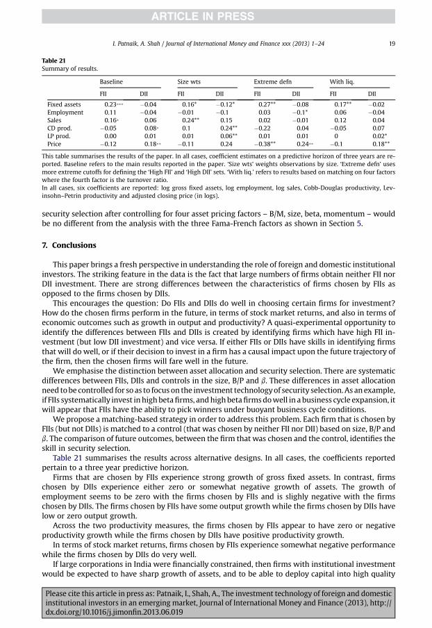
Table 21Summary of results.
Baseline Size wts Extreme defn With liq.
FII DII FII DII FII DII FII DII
Fixed assets 0.23*** �0.04 0.16* �0.12* 0.27** �0.08 0.17** �0.02Employment 0.11 �0.04 �0.01 �0.1 0.03 �0.1* 0.06 �0.04Sales 0.16* 0.06 0.24** 0.15 0.02 �0.01 0.12 0.04CD prod. �0.05 0.08* 0.1 0.24** �0.22 0.04 �0.05 0.07LP prod. 0.00 0.01 0.01 0.06** 0.01 0.01 0 0.02*Price �0.12 0.18** �0.11 0.24 �0.38** 0.24** �0.1 0.18**
This table summarises the results of the paper. In all cases, coefficient estimates on a predictive horizon of three years are re-ported. Baseline refers to the main results reported in the paper. ‘Size wts’ weights observations by size. ‘Extreme defn’ usesmore extreme cutoffs for defining the ‘High FII’ and ‘High DII’ sets. ‘With liq.’ refers to results based on matching on four factorswhere the fourth factor is the turnover ratio.In all cases, six coefficients are reported: log gross fixed assets, log employment, log sales, Cobb-Douglas productivity, Lev-insohn–Petrin productivity and adjusted closing price (in logs).
I. Patnaik, A. Shah / Journal of International Money and Finance xxx (2013) 1–24 19
security selection after controlling for four asset pricing factors – B/M, size, beta, momentum – wouldbe no different from the analysis with the three Fama-French factors as shown in Section 5.
7. Conclusions
This paper brings a fresh perspective in understanding the role of foreign and domestic institutionalinvestors. The striking feature in the data is the fact that large numbers of firms obtain neither FII norDII investment. There are strong differences between the characteristics of firms chosen by FIIs asopposed to the firms chosen by DIIs.
This encourages the question: Do FIIs and DIIs do well in choosing certain firms for investment?How do the chosen firms perform in the future, in terms of stock market returns, and also in terms ofeconomic outcomes such as growth in output and productivity? A quasi-experimental opportunity toidentify the differences between FIIs and DIIs is created by identifying firms which have high FII in-vestment (but low DII investment) and vice versa. If either FIIs or DIIs have skills in identifying firmsthat will do well, or if their decision to invest in a firm has a causal impact upon the future trajectory ofthe firm, then the chosen firms will fare well in the future.
We emphasise the distinction between asset allocation and security selection. There are systematicdifferences between FIIs, DIIs and controls in the size, B/P and b. These differences in asset allocationneed tobe controlled for so as to focuson the investment technologyof security selection.As anexample,if FIIs systematically invest inhighbetafirms, andhighbetafirmsdowell in a business cycle expansion, itwill appear that FIIs have the ability to pick winners under buoyant business cycle conditions.
We propose a matching-based strategy in order to address this problem. Each firm that is chosen byFIIs (but not DIIs) is matched to a control (that was chosen by neither FII nor DII) based on size, B/P andb. The comparison of future outcomes, between the firm that was chosen and the control, identifies theskill in security selection.
Table 21 summarises the results across alternative designs. In all cases, the coefficients reportedpertain to a three year predictive horizon.
Firms that are chosen by FIIs experience strong growth of gross fixed assets. In contrast, firmschosen by DIIs experience either zero or somewhat negative growth of assets. The growth ofemployment seems to be zero with the firms chosen by FIIs and is slighly negative with the firmschosen by DIIs. The firms chosen by FIIs have some output growth while the firms chosen by DIIs havelow or zero output growth.
Across the two productivity measures, the firms chosen by FIIs appear to have zero or negativeproductivity growth while the firms chosen by DIIs have positive productivity growth.
In terms of stock market returns, firms chosen by FIIs experience somewhat negative performancewhile the firms chosen by DIIs do very well.
If large corporations in India were financially constrained, then firms with institutional investmentwould be expected to have sharp growth of assets, and to be able to deploy capital into high quality
Please cite this article in press as: Patnaik, I., Shah, A., The investment technology of foreign and domesticinstitutional investors in an emerging market, Journal of International Money and Finance (2013), http://dx.doi.org/10.1016/j.jimonfin.2013.06.019
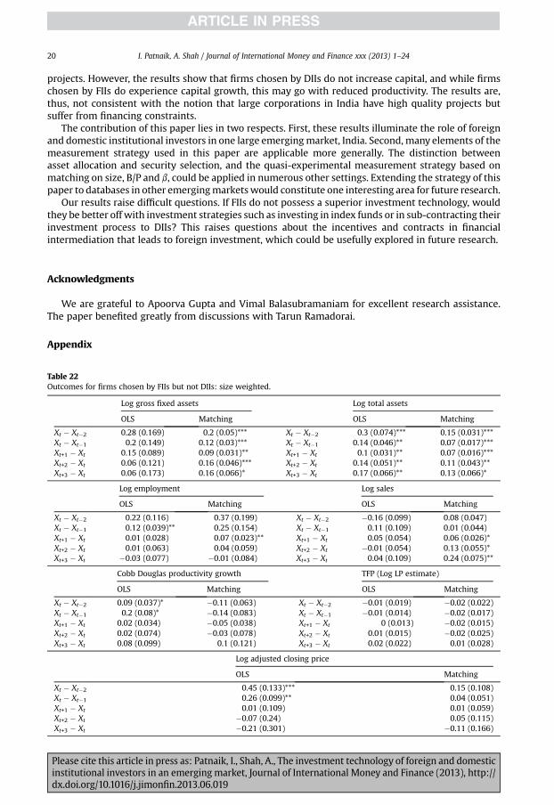
I. Patnaik, A. Shah / Journal of International Money and Finance xxx (2013) 1–2420
projects. However, the results show that firms chosen by DIIs do not increase capital, and while firmschosen by FIIs do experience capital growth, this may go with reduced productivity. The results are,thus, not consistent with the notion that large corporations in India have high quality projects butsuffer from financing constraints.
The contribution of this paper lies in two respects. First, these results illuminate the role of foreignand domestic institutional investors in one large emergingmarket, India. Second, many elements of themeasurement strategy used in this paper are applicable more generally. The distinction betweenasset allocation and security selection, and the quasi-experimental measurement strategy based onmatching on size, B/P and b, could be applied in numerous other settings. Extending the strategy of thispaper to databases in other emergingmarketswould constitute one interesting area for future research.
Our results raise difficult questions. If FIIs do not possess a superior investment technology, wouldthey be better off with investment strategies such as investing in index funds or in sub-contracting theirinvestment process to DIIs? This raises questions about the incentives and contracts in financialintermediation that leads to foreign investment, which could be usefully explored in future research.
Acknowledgments
We are grateful to Apoorva Gupta and Vimal Balasubramaniam for excellent research assistance.The paper benefited greatly from discussions with Tarun Ramadorai.
Appendix
Table 22Outcomes for firms chosen by FIIs but not DIIs: size weighted.
Log gross fixed assets Log total assets
OLS Matching OLS Matching
Xt � Xt�2 0.28 (0.169) 0.2 (0.05)*** Xt � Xt�2 0.3 (0.074)*** 0.15 (0.031)***Xt � Xt�1 0.2 (0.149) 0.12 (0.03)*** Xt � Xt�1 0.14 (0.046)** 0.07 (0.017)***Xt+1 � Xt 0.15 (0.089) 0.09 (0.031)** Xt+1 � Xt 0.1 (0.031)** 0.07 (0.016)***Xt+2 � Xt 0.06 (0.121) 0.16 (0.046)*** Xt+2 � Xt 0.14 (0.051)** 0.11 (0.043)**Xt+3 � Xt 0.06 (0.173) 0.16 (0.066)* Xt+3 � Xt 0.17 (0.066)** 0.13 (0.066)*
Log employment Log sales
OLS Matching OLS Matching
Xt � Xt�2 0.22 (0.116) 0.37 (0.199) Xt � Xt�2 �0.16 (0.099) 0.08 (0.047)Xt � Xt�1 0.12 (0.039)** 0.25 (0.154) Xt � Xt�1 0.11 (0.109) 0.01 (0.044)Xt+1 � Xt 0.01 (0.028) 0.07 (0.023)** Xt+1 � Xt 0.05 (0.054) 0.06 (0.026)*Xt+2 � Xt 0.01 (0.063) 0.04 (0.059) Xt+2 � Xt �0.01 (0.054) 0.13 (0.055)*Xt+3 � Xt �0.03 (0.077) �0.01 (0.084) Xt+3 � Xt 0.04 (0.109) 0.24 (0.075)**
Cobb Douglas productivity growth TFP (Log LP estimate)
OLS Matching OLS Matching
Xt � Xt�2 0.09 (0.037)* �0.11 (0.063) Xt � Xt�2 �0.01 (0.019) �0.02 (0.022)Xt � Xt�1 0.2 (0.08)* �0.14 (0.083) Xt � Xt�1 �0.01 (0.014) �0.02 (0.017)Xt+1 � Xt 0.02 (0.034) �0.05 (0.038) Xt+1 � Xt 0 (0.013) �0.02 (0.015)Xt+2 � Xt 0.02 (0.074) �0.03 (0.078) Xt+2 � Xt 0.01 (0.015) �0.02 (0.025)Xt+3 � Xt 0.08 (0.099) 0.1 (0.121) Xt+3 � Xt 0.02 (0.022) 0.01 (0.028)
Log adjusted closing price
OLS Matching
Xt � Xt�2 0.45 (0.133)*** 0.15 (0.108)Xt � Xt�1 0.26 (0.099)** 0.04 (0.051)Xt+1 � Xt 0.01 (0.109) 0.01 (0.059)Xt+2 � Xt �0.07 (0.24) 0.05 (0.115)Xt+3 � Xt �0.21 (0.301) �0.11 (0.166)
Please cite this article in press as: Patnaik, I., Shah, A., The investment technology of foreign and domesticinstitutional investors in an emerging market, Journal of International Money and Finance (2013), http://dx.doi.org/10.1016/j.jimonfin.2013.06.019
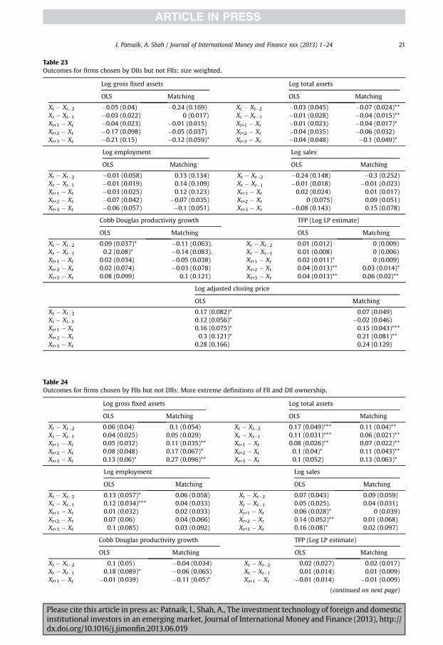
Table 24Outcomes for firms chosen by FIIs but not DIIs: More extreme definitions of FII and DII ownership.
Log gross fixed assets Log total assets
OLS Matching OLS Matching
Xt � Xt�2 0.06 (0.04) 0.1 (0.054) Xt � Xt�2 0.17 (0.049)*** 0.11 (0.04)**Xt � Xt�1 0.04 (0.025) 0.05 (0.029) Xt � Xt�1 0.11 (0.031)*** 0.06 (0.021)**Xt+1 � Xt 0.05 (0.032) 0.11 (0.035)** Xt+1 � Xt 0.08 (0.026)** 0.07 (0.022)**Xt+2 � Xt 0.08 (0.048) 0.17 (0.067)* Xt+2 � Xt 0.1 (0.04)* 0.11 (0.043)**Xt+3 � Xt 0.13 (0.06)* 0.27 (0.096)** Xt+3 � Xt 0.1 (0.052) 0.13 (0.063)*
Log employment Log sales
OLS Matching OLS Matching
Xt � Xt�2 0.13 (0.057)* 0.06 (0.058) Xt � Xt�2 0.07 (0.043) 0.09 (0.059)Xt � Xt�1 0.12 (0.034)*** 0.04 (0.033) Xt � Xt�1 0.05 (0.025). 0.04 (0.031)Xt+1 � Xt 0.01 (0.032) 0.02 (0.033) Xt+1 � Xt 0.06 (0.028)* 0 (0.039)Xt+2 � Xt 0.07 (0.06) 0.04 (0.066) Xt+2 � Xt 0.14 (0.052)** 0.01 (0.068)Xt+3 � Xt 0.1 (0.085) 0.03 (0.092) Xt+3 � Xt 0.16 (0.08)* 0.02 (0.097)
Cobb Douglas productivity growth TFP (Log LP estimate)
OLS Matching OLS Matching
Xt � Xt�2 0.1 (0.05) �0.04 (0.034) Xt � Xt�2 0.02 (0.027) 0.02 (0.017)Xt � Xt�1 0.18 (0.089)* �0.06 (0.065) Xt � Xt�1 0.01 (0.014) 0.01 (0.009)Xt+1 � Xt �0.01 (0.039) �0.11 (0.05)* Xt+1 � Xt �0.01 (0.014) �0.01 (0.009)
(continued on next page)
Table 23Outcomes for firms chosen by DIIs but not FIIs: size weighted.
Log gross fixed assets Log total assets
OLS Matching OLS Matching
Xt � Xt�2 �0.05 (0.04) �0.24 (0.169) Xt � Xt�2 �0.03 (0.045) �0.07 (0.024)**Xt � Xt�1 �0.03 (0.022) 0 (0.017) Xt � Xt�1 �0.01 (0.028) �0.04 (0.015)**Xt+1 � Xt �0.04 (0.023) �0.01 (0.015) Xt+1 � Xt �0.01 (0.023) �0.04 (0.017)*Xt+2 � Xt �0.17 (0.098) �0.05 (0.037) Xt+2 � Xt �0.04 (0.035) �0.06 (0.032)Xt+3 � Xt �0.21 (0.15) �0.12 (0.059)* Xt+3 � Xt �0.04 (0.048) �0.1 (0.049)*
Log employment Log sales
OLS Matching OLS Matching
Xt � Xt�2 �0.01 (0.058) 0.13 (0.134) Xt � Xt�2 �0.24 (0.148) �0.3 (0.252)Xt � Xt�1 �0.01 (0.019) 0.14 (0.109) Xt � Xt�1 �0.01 (0.018) �0.01 (0.023)Xt+1 � Xt �0.03 (0.025) 0.12 (0.123) Xt+1 � Xt 0.02 (0.024) 0.01 (0.017)Xt+2 � Xt �0.07 (0.042) �0.07 (0.035) Xt+2 � Xt 0 (0.075) 0.09 (0.051)Xt+3 � Xt �0.06 (0.057) �0.1 (0.051) Xt+3 � Xt �0.08 (0.143) 0.15 (0.078)
Cobb Douglas productivity growth TFP (Log LP estimate)
OLS Matching OLS Matching
Xt � Xt�2 0.09 (0.037)* �0.11 (0.063). Xt � Xt�2 0.01 (0.012) 0 (0.009)Xt � Xt�1 0.2 (0.08)* �0.14 (0.083). Xt � Xt�1 0.01 (0.008) 0 (0.006)Xt+1 � Xt 0.02 (0.034) �0.05 (0.038) Xt+1 � Xt 0.02 (0.011)* 0 (0.009)Xt+2 � Xt 0.02 (0.074) �0.03 (0.078) Xt+2 � Xt 0.04 (0.013)** 0.03 (0.014)*Xt+3 � Xt 0.08 (0.099) 0.1 (0.121) Xt+3 � Xt 0.04 (0.013)** 0.06 (0.02)**
Log adjusted closing price
OLS Matching
Xt � Xt�2 0.17 (0.082)* 0.07 (0.049)Xt � Xt�1 0.12 (0.056)* �0.02 (0.046)Xt+1 � Xt 0.16 (0.075)* 0.15 (0.043)***Xt+2 � Xt 0.3 (0.121)* 0.21 (0.081)**Xt+3 � Xt 0.28 (0.166) 0.24 (0.129)
Please cite this article in press as: Patnaik, I., Shah, A., The investment technology of foreign and domesticinstitutional investors in an emerging market, Journal of International Money and Finance (2013), http://dx.doi.org/10.1016/j.jimonfin.2013.06.019
I. Patnaik, A. Shah / Journal of International Money and Finance xxx (2013) 1–24 21
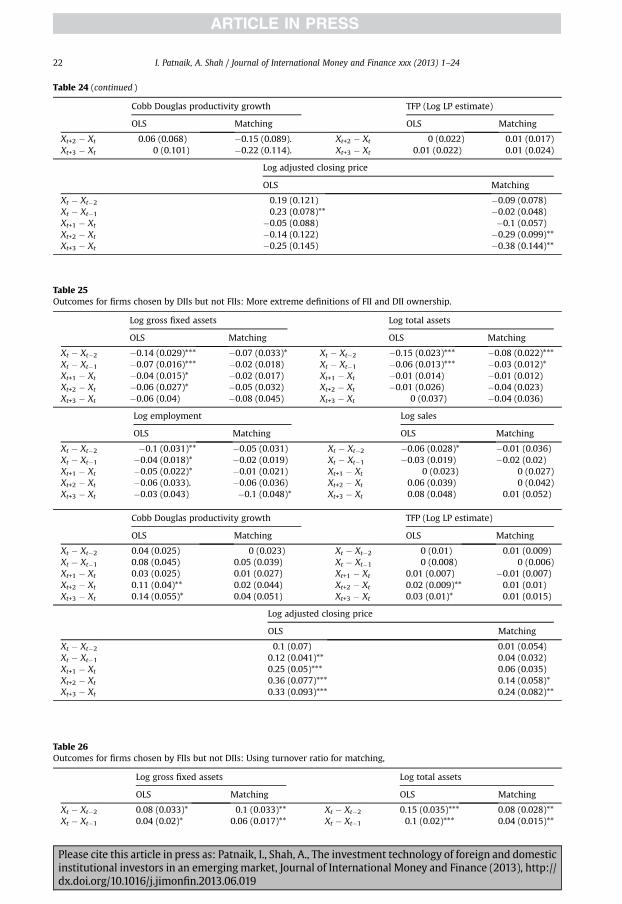
Table 25Outcomes for firms chosen by DIIs but not FIIs: More extreme definitions of FII and DII ownership.
Log gross fixed assets Log total assets
OLS Matching OLS Matching
Xt � Xt�2 �0.14 (0.029)*** �0.07 (0.033)* Xt � Xt�2 �0.15 (0.023)*** �0.08 (0.022)***Xt � Xt�1 �0.07 (0.016)*** �0.02 (0.018) Xt � Xt�1 �0.06 (0.013)*** �0.03 (0.012)*Xt+1 � Xt �0.04 (0.015)* �0.02 (0.017) Xt+1 � Xt �0.01 (0.014) �0.01 (0.012)Xt+2 � Xt �0.06 (0.027)* �0.05 (0.032) Xt+2 � Xt �0.01 (0.026) �0.04 (0.023)Xt+3 � Xt �0.06 (0.04) �0.08 (0.045) Xt+3 � Xt 0 (0.037) �0.04 (0.036)
Log employment Log sales
OLS Matching OLS Matching
Xt � Xt�2 �0.1 (0.031)** �0.05 (0.031) Xt � Xt�2 �0.06 (0.028)* �0.01 (0.036)Xt � Xt�1 �0.04 (0.018)* �0.02 (0.019) Xt � Xt�1 �0.03 (0.019) �0.02 (0.02)Xt+1 � Xt �0.05 (0.022)* �0.01 (0.021) Xt+1 � Xt 0 (0.023) 0 (0.027)Xt+2 � Xt �0.06 (0.033). �0.06 (0.036) Xt+2 � Xt 0.06 (0.039) 0 (0.042)Xt+3 � Xt �0.03 (0.043) �0.1 (0.048)* Xt+3 � Xt 0.08 (0.048) 0.01 (0.052)
Cobb Douglas productivity growth TFP (Log LP estimate)
OLS Matching OLS Matching
Xt � Xt�2 0.04 (0.025) 0 (0.023) Xt � Xt�2 0 (0.01) 0.01 (0.009)Xt � Xt�1 0.08 (0.045) 0.05 (0.039) Xt � Xt�1 0 (0.008) 0 (0.006)Xt+1 � Xt 0.03 (0.025) 0.01 (0.027) Xt+1 � Xt 0.01 (0.007) �0.01 (0.007)Xt+2 � Xt 0.11 (0.04)** 0.02 (0.044) Xt+2 � Xt 0.02 (0.009)** 0.01 (0.01)Xt+3 � Xt 0.14 (0.055)* 0.04 (0.051) Xt+3 � Xt 0.03 (0.01)* 0.01 (0.015)
Log adjusted closing price
OLS Matching
Xt � Xt�2 0.1 (0.07) 0.01 (0.054)Xt � Xt�1 0.12 (0.041)** 0.04 (0.032)Xt+1 � Xt 0.25 (0.05)*** 0.06 (0.035)Xt+2 � Xt 0.36 (0.077)*** 0.14 (0.058)*Xt+3 � Xt 0.33 (0.093)*** 0.24 (0.082)**
Table 24 (continued )
Cobb Douglas productivity growth TFP (Log LP estimate)
OLS Matching OLS Matching
Xt+2 � Xt 0.06 (0.068) �0.15 (0.089). Xt+2 � Xt 0 (0.022) 0.01 (0.017)Xt+3 � Xt 0 (0.101) �0.22 (0.114). Xt+3 � Xt 0.01 (0.022) 0.01 (0.024)
Log adjusted closing price
OLS Matching
Xt � Xt�2 0.19 (0.121) �0.09 (0.078)Xt � Xt�1 0.23 (0.078)** �0.02 (0.048)Xt+1 � Xt �0.05 (0.088) �0.1 (0.057)Xt+2 � Xt �0.14 (0.122) �0.29 (0.099)**Xt+3 � Xt �0.25 (0.145) �0.38 (0.144)**
Table 26Outcomes for firms chosen by FIIs but not DIIs: Using turnover ratio for matching,
Log gross fixed assets Log total assets
OLS Matching OLS Matching
Xt � Xt�2 0.08 (0.033)* 0.1 (0.033)** Xt � Xt�2 0.15 (0.035)*** 0.08 (0.028)**Xt � Xt�1 0.04 (0.02)* 0.06 (0.017)** Xt � Xt�1 0.1 (0.02)*** 0.04 (0.015)**
Please cite this article in press as: Patnaik, I., Shah, A., The investment technology of foreign and domesticinstitutional investors in an emerging market, Journal of International Money and Finance (2013), http://dx.doi.org/10.1016/j.jimonfin.2013.06.019
I. Patnaik, A. Shah / Journal of International Money and Finance xxx (2013) 1–2422
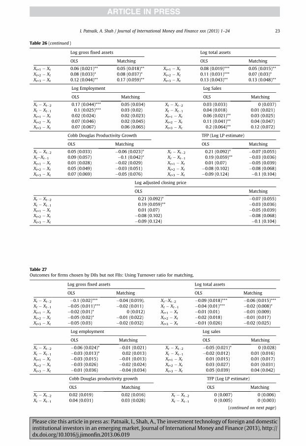
Table 27Outcomes for firms chosen by DIIs but not FIIs: Using Turnover ratio for matching,
Log gross fixed assets Log total assets
OLS Matching OLS Matching
Xt � Xt�2 �0.1 (0.02)*** �0.04 (0.019). Xt�Xt�2 �0.09 (0.018)*** �0.06 (0.015)***Xt � Xt�1 �0.05 (0.011)*** �0.02 (0.011) Xt � Xt�1 �0.04 (0.01)*** �0.02 (0.008)*Xt+1 � Xt �0.02 (0.01)* 0 (0.012) Xt+1 � Xt �0.01 (0.01) �0.01 (0.009)Xt+2 � Xt �0.05 (0.02)* �0.01 (0.022) Xt+2 � Xt �0.02 (0.018) �0.01 (0.017)Xt+3 � Xt �0.05 (0.03) �0.02 (0.032) Xt+3 � Xt �0.01 (0.026) �0.02 (0.025)
Log employment Log sales
OLS Matching OLS Matching
Xt � Xt�2 �0.06 (0.024)* �0.01 (0.021) Xt � Xt�2 �0.05 (0.021)* 0 (0.028)Xt � Xt�1 �0.03 (0.013)* 0.02 (0.013) Xt � Xt�1 �0.02 (0.012) 0.01 (0.016)Xt+1 � Xt �0.03 (0.015) �0.01 (0.013) Xt+1 � Xt 0.01 (0.015) 0.01 (0.017)Xt+2 � Xt �0.03 (0.026) �0.02 (0.024) Xt+2 � Xt 0.03 (0.027) 0.01 (0.031)Xt+3 � Xt �0.01 (0.036) �0.04 (0.034) Xt+3 � Xt 0.05 (0.039) 0.04 (0.042)
Cobb Douglas productivity growth TFP (Log LP estimate)
OLS Matching OLS Matching
Xt � Xt�2 0.02 (0.019) 0.02 (0.016) Xt � Xt�2 0 (0.007) 0 (0.006)Xt � Xt�1 0.04 (0.031) 0.03 (0.028) Xt � Xt�1 0 (0.005) 0 (0.003)
(continued on next page)
Table 26 (continued )
Log gross fixed assets Log total assets
OLS Matching OLS Matching
Xt+1 � Xt 0.06 (0.021)** 0.05 (0.018)** Xt+1 � Xt 0.08 (0.019)*** 0.05 (0.015)**Xt+2 � Xt 0.08 (0.033)* 0.08 (0.037)* Xt+2 � Xt 0.11 (0.031)*** 0.07 (0.03)*Xt+3 � Xt 0.12 (0.044)** 0.17 (0.059)** Xt+3 � Xt 0.13 (0.043)** 0.13 (0.048)**
Log Employment Log Sales
OLS Matching OLS Matching
Xt � Xt�2 0.17 (0.044)*** 0.05 (0.034) Xt � Xt�2 0.03 (0.033) 0 (0.037)Xt � Xt�1 0.1 (0.025)*** 0.03 (0.02) Xt � Xt�1 0.04 (0.018) 0.01 (0.021)Xt+1 � Xt 0.02 (0.024) 0.02 (0.023) Xt+1 � Xt 0.06 (0.021)** 0.03 (0.025)Xt+2 � Xt 0.07 (0.046) 0.02 (0.045) Xt+2 � Xt 0.11 (0.041)** 0.04 (0.047)Xt+3 � Xt 0.07 (0.067) 0.06 (0.065) Xt+3 � Xt 0.2 (0.064)** 0.12 (0.072)
Cobb Douglas Productivity Growth TFP (Log LP estimate)
OLS Matching OLS Matching
Xt � Xt�2 0.05 (0.033) �0.06 (0.023)* Xt � Xt�2 0.21 (0.092)* �0.07 (0.055)Xt�Xt�1 0.09 (0.057) �0.1 (0.042)* Xt � Xt�1 0.19 (0.059)** �0.03 (0.036)Xt+1 � Xt 0.01 (0.028) �0.02 (0.029) Xt+1 � Xt 0.01 (0.07) �0.05 (0.039)Xt+2 � Xt 0.05 (0.049) �0.03 (0.051) Xt+2 � Xt �0.08 (0.102) �0.08 (0.068)Xt+3 � Xt 0.07 (0.069) �0.05 (0.076) Xt+3 � Xt �0.09 (0.124) �0.1 (0.104)
Log adjusted closing price
OLS Matching
Xt � Xt�2 0.21 (0.092)* �0.07 (0.055)Xt � Xt�1 0.19 (0.059)** �0.03 (0.036)Xt+1 � Xt 0.01 (0.07) �0.05 (0.039)Xt+2 � Xt �0.08 (0.102) �0.08 (0.068)Xt+3 � Xt �0.09 (0.124) �0.1 (0.104)
I. Patnaik, A. Shah / Journal of International Money and Finance xxx (2013) 1–24 23
Please cite this article in press as: Patnaik, I., Shah, A., The investment technology of foreign and domesticinstitutional investors in an emerging market, Journal of International Money and Finance (2013), http://dx.doi.org/10.1016/j.jimonfin.2013.06.019
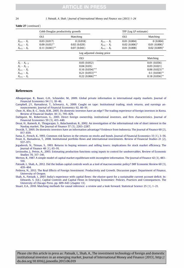
Table 27 (continued )
Cobb Douglas productivity growth TFP (Log LP estimate)
OLS Matching OLS Matching
Xt+1 � Xt 0.03 (0.017) 0 (0.018) Xt+1 � Xt 0.01 (0.004) 0 (0.004)Xt+2 � Xt 0.09 (0.03)** 0.02 (0.029) Xt+2 � Xt 0.02 (0.006)* 0.01 (0.006)*Xt+3 � Xt 0.11 (0.041)** 0.07 (0.041) Xt+3 � Xt 0.01 (0.008) 0.02 (0.009)*
Log adjusted closing price
OLS Matching
Xt � Xt�2 0.05 (0.052) 0.01 (0.036)Xt � Xt�1 0.04 (0.03) 0.03 (0.021)Xt+1 � Xt 0.16 (0.034)*** 0.06 (0.023)**Xt+2 � Xt 0.21 (0.053)*** 0.1 (0.038)**Xt+3 � Xt 0.22 (0.066)*** 0.18 (0.056)**
I. Patnaik, A. Shah / Journal of International Money and Finance xxx (2013) 1–2424
References
Albuquerque, R., Bauer, G.H., Schneider, M., 2009. Global private information in international equity markets. Journal ofFinancial Economics 94 (1), 18–46.
Campbell, J.Y., Ramadorai, T., Schwartz, A., 2009. Caught on tape: Institutional trading, stock returns, and earnings an-nouncements. Journal of Financial Economics 92, 66–91.
Choe, H., Kho, B.-C., Stulz, R.M., 2005. Do domestic investors have an edge? The trading experience of foreign investors in Korea.Review of Financial Studies 18 (3), 795–829.
Dahlquist, M., Robertsson, G., 2001. Direct foreign ownership, institutional investors, and firm characteristics. Journal ofFinancial Economics 59 (3), 413–440.
Desai, H., Ramesh, K., Thiagarajan, S., Balachandran, B., 2002. An investigation of the informational role of short interest in theNasdaq market. The Journal of Finance 57 (5), 2263–2287.
Dvo�rák, T., 2005. Do domestic investors have an information advantage? Evidence from Indonesia. The Journal of Finance 60 (2),817–839.
Fama, E., French, K., 1993. Common risk factors in the returns on stocks and bonds. Journal of Financial Economics 33 (1), 3–56.Froot, K., Ramadorai, T., 2008. Institutional portfolio flows and international investments. Review of Financial Studies 21 (2),
937–971.Jegadeesh, N., Titman, S., 1993. Returns to buying winners and selling losers: implications for stock market efficiency. The
Journal of Finance 48 (1), 65–91.Levinsohn, J., Petrin, A., 2003. Estimating production functions using inputs to control for unobservables. Review of Economic
Studies 70, 317–341.Merton, R., 1987. A simple model of capital market equilibriumwith incomplete information. The Journal of Finance 42 (3), 483–
510.Patnaik, I., Shah, A., 2012. Did the Indian capital controls work as a tool of macroeconomic policy? IMF Economic Review 60 (3),
439–464.Petkova, N., 2012. The Real Effects of Foreign Investment: Productivity and Growth. Discussion paper. Department of Finance,
University of Oregon.Shah, A., Patnaik, I., 2007. India’s experience with capital flows: the elusive quest for a sustainable current account deficit. In:
Edwards, S. (Ed.), Capital Controls and Capital Flows in Emerging Economies: Policies, Practices and Consequences. TheUniversity of Chicago Press, pp. 609–643 (chapter 13).
Stuart, E.A., 2010. Matching methods for causal inference: a review and a look forward. Statistical Science 25 (1), 1–21.
Please cite this article in press as: Patnaik, I., Shah, A., The investment technology of foreign and domesticinstitutional investors in an emerging market, Journal of International Money and Finance (2013), http://dx.doi.org/10.1016/j.jimonfin.2013.06.019