Contact Pressure Distribution Optimization

George R. Hric III

Thesis submitted to the faculty of the Virginia Polytechnic and State University in partial ful�llment of the

requirements for the degree of:

Master of ScienceIn

Mechanical Engineering

Willem G. Odendaal

Alfred Wicks

Brian Vick

May 4th 2016

Blacksburg, VA

Keywords: Contact, Pressure Distribution, Pulsed Power

Copyright 2016

Contact Pressure Distribution Optimization

George R. Hric III

ABSTRACT

A novel design technique that is used to optimize contact pressure distribution was introduced and

investigated. The primary objective of this design tool, called the Predicted Displacement Method, was

to provide a calculated contact surface shape alteration of a contact body that induces a uniform contact

pressure across its entire nominal contact surface when pressed against its destination contact boundary at

a speci�ed magnitude. This technique was developed so it could be applied to any contact surface to spread

out a once poorly distributed and localized contact pressure distribution. The methodology was detailed in

this work and a proof of concept was conducted to test the idea's feasibility. The proof of concept supported

the methodology's ability to shape a cantilevered beam so that it pressed against a semi-in�nite space

uniformly. This methodology was then applied to two relevant contact assemblies and resulted in uniform

contact across each contact interface. The results also illustrated the ability to control contact magnitude

and demonstrated improved contact distribution at magnitudes beyond the design value. The methodology

presented in this work provides engineers with a analytical and numerical tool to improve contact pressure

distribution between any contact surfaces. Possible future use of this methodology includes incorporation

into engineering software packages for contact surface design.

Contact Pressure Distribution Optimization

George R. Hric III

GENERAL AUDIENCE ABSTRACT

When two objects are squeezed together, their contacting surfaces deform in a manner that produces

uneven contact pressure, causing some of the object's surface area to be pressed together harder than

others. This uneven distribution of pressure can have negative e�ects on electrical conductivity and overall

mechanical performance. The work presented here introduces a technique that helps remedy this uneven

contact pressure by precisely shaping the object's contact surface. It was found that, by using computational

software, one could solve for the exact surface shape an object needs to provide even contact pressure across

its entire surface area. The idea was tested through computer simulations and the results showed a drastic

improvement of contact pressure distribution.

Acknowledgments

I would like to like to give a tremendous thanks to my adviser, Professor Hardus Odendaal, for his unwavering

support of my research and studies. Words can not describe my gratitude for the opportunity of being a

part of his research program through out my graduate and undergraduate years. The time spent working in

his lab was challenging, exciting, fun, and de�ned my academic career.

I would like to thank my committee members, Professor Al Wicks and Professor Brian Vick, for their

encouragement, time, and patience.

My sincere thanks also goes to Victor Sung for his insight, suggestions, and assistance in my research.

His contributions to my work in the lab and research were invaluable.

Lastly, I would like to thank my parents, George and Michele Hric, for their crucial support and guidance

through out my academic career.

iv

Contents

1 Introduction 1

1.1 Background . . . . . . . . . . . . . . . . . . . . . . . . . . . . . . . . . . . . . . . . . . . . . . 1

1.2 Motivation . . . . . . . . . . . . . . . . . . . . . . . . . . . . . . . . . . . . . . . . . . . . . . 2

1.2.1 Joule Heating . . . . . . . . . . . . . . . . . . . . . . . . . . . . . . . . . . . . . . . . . 2

1.2.2 Electrical Blow O� . . . . . . . . . . . . . . . . . . . . . . . . . . . . . . . . . . . . . . 3

1.3 Scope . . . . . . . . . . . . . . . . . . . . . . . . . . . . . . . . . . . . . . . . . . . . . . . . . 5

2 Literature Review 5

3 Contact Theory 6

3.1 Hertzian Contact . . . . . . . . . . . . . . . . . . . . . . . . . . . . . . . . . . . . . . . . . . 6

3.2 Computational Contact Mechanics . . . . . . . . . . . . . . . . . . . . . . . . . . . . . . . . . 7

3.2.1 Model Formulation . . . . . . . . . . . . . . . . . . . . . . . . . . . . . . . . . . . . . . 7

3.2.2 Lagrange Multiplier Method . . . . . . . . . . . . . . . . . . . . . . . . . . . . . . . . . 9

3.2.3 Penalty Method . . . . . . . . . . . . . . . . . . . . . . . . . . . . . . . . . . . . . . . 10

3.2.4 Application . . . . . . . . . . . . . . . . . . . . . . . . . . . . . . . . . . . . . . . . . . 10

4 Predicted Displacement Method 11

4.1 Theory . . . . . . . . . . . . . . . . . . . . . . . . . . . . . . . . . . . . . . . . . . . . . . . . . 12

4.1.1 Assumptions . . . . . . . . . . . . . . . . . . . . . . . . . . . . . . . . . . . . . . . . . 12

4.1.2 Linear Elastic Behavior . . . . . . . . . . . . . . . . . . . . . . . . . . . . . . . . . . . 12

4.1.3 Euler-Bernoulli Beam De�ection . . . . . . . . . . . . . . . . . . . . . . . . . . . . . . 14

4.1.4 Timoshenko Beam De�ection . . . . . . . . . . . . . . . . . . . . . . . . . . . . . . . . 15

4.2 Analytical Approach . . . . . . . . . . . . . . . . . . . . . . . . . . . . . . . . . . . . . . . . . 16

4.2.1 Conclusions . . . . . . . . . . . . . . . . . . . . . . . . . . . . . . . . . . . . . . . . . . 16

4.3 Methodology . . . . . . . . . . . . . . . . . . . . . . . . . . . . . . . . . . . . . . . . . . . . . 17

4.4 Proof of Concept . . . . . . . . . . . . . . . . . . . . . . . . . . . . . . . . . . . . . . . . . . . 17

4.4.1 Model Setup . . . . . . . . . . . . . . . . . . . . . . . . . . . . . . . . . . . . . . . . . 18

4.4.2 PDM Shape . . . . . . . . . . . . . . . . . . . . . . . . . . . . . . . . . . . . . . . . . . 21

4.4.3 Simulation Setup . . . . . . . . . . . . . . . . . . . . . . . . . . . . . . . . . . . . . . . 22

4.4.4 Results . . . . . . . . . . . . . . . . . . . . . . . . . . . . . . . . . . . . . . . . . . . . 25

4.4.5 Conclusions . . . . . . . . . . . . . . . . . . . . . . . . . . . . . . . . . . . . . . . . . . 30

iv

5 Applications and Results 32

5.1 Thin Cylinders . . . . . . . . . . . . . . . . . . . . . . . . . . . . . . . . . . . . . . . . . . . . 32

5.2 Prism and Plate Clamp . . . . . . . . . . . . . . . . . . . . . . . . . . . . . . . . . . . . . . . 37

6 Conclusions 42

References 44

v

List of Figures

1 Current �owing through contacting asperities (2D Side View) . . . . . . . . . . . . . . . . . . 4

2 Mass spring system . . . . . . . . . . . . . . . . . . . . . . . . . . . . . . . . . . . . . . . . . 8

3 De�ection comparison between beams in bending. Straight beam (top) de�ects same as non-

straight beam (bottom) . . . . . . . . . . . . . . . . . . . . . . . . . . . . . . . . . . . . . . . 11

4 Comparison between axial de�ection from load and reaction force from forced de�ection . . . 14

5 Illustration of beam and establishment of coordinate system . . . . . . . . . . . . . . . . . . . 18

6 General beam contact simulation setup . . . . . . . . . . . . . . . . . . . . . . . . . . . . . . . 19

7 Residual of PDM shaped beam and 4th order curve �t of PDM shape . . . . . . . . . . . . . 20

8 Visual representation of load on contact prism (a) and cantilevered beam (b) . . . . . . . . . 21

9 Surface deformation result of prism;s (a) and cantilevered beam's (b) contact surface . . . . . 22

10 COMSOL beam contact geometry de�nitions . . . . . . . . . . . . . . . . . . . . . . . . . . . 24

11 Meshing scheme used in beam contact simulations . . . . . . . . . . . . . . . . . . . . . . . . 25

12 Von Mises stress plot of linear shaped beam in contact with prism . . . . . . . . . . . . . . . 26

13 Zoomed-in view of labeled area in Fig. 12 . . . . . . . . . . . . . . . . . . . . . . . . . . . . . 26

14 Von Mises stress plot of PDM shaped beam in contact with prism . . . . . . . . . . . . . . . 26

15 Resulting contact pressure between linear (a) convex (b) concave (c) PDM (d) shaped beams

and prism . . . . . . . . . . . . . . . . . . . . . . . . . . . . . . . . . . . . . . . . . . . . . . . 27

16 Zoomed in contact plot from Fig. 15(d) . . . . . . . . . . . . . . . . . . . . . . . . . . . . . . 28

17 Extruded contact results displayed in Fig. 15 . . . . . . . . . . . . . . . . . . . . . . . . . . . 29

18 Resulting contact pressure of di�erent linearly shaped beam . . . . . . . . . . . . . . . . . . . 30

19 Resulting contact pressure from beam shaped as a 4th order PDM approximation . . . . . . 30

20 Illustration of contact scenario . . . . . . . . . . . . . . . . . . . . . . . . . . . . . . . . . . . 32

21 Axisymmetrical contact distribution simulation result of two perfect cylinders squeezed by

concentric nut, washer, bolt assembly . . . . . . . . . . . . . . . . . . . . . . . . . . . . . . . . 33

22 Contact pressure in respect to disk radii along nominal contact surface . . . . . . . . . . . . . 33

23 Gap between two cylinders as a function of radius when nut, washer, bolt assembly at 200N . 34

24 Contact pressure at di�erent assembly loads . . . . . . . . . . . . . . . . . . . . . . . . . . . . 35

25 Gap between disks at di�erent assembly loads . . . . . . . . . . . . . . . . . . . . . . . . . . . 35

26 Exaggerated illustration of PDM shaped disk beginning contact with cylindrical disk . . . . . 36

27 Contact pressure as a function of disk radii between PDM and regular disks . . . . . . . . . . 36

v

28 Contact pressure results at di�erent assembly loads. Note ideal contact at design load and

non-zero contact at all loads contrasts Fig. 24 results . . . . . . . . . . . . . . . . . . . . . . . 37

29 Example illustration of pulse power transfer contact assembly . . . . . . . . . . . . . . . . . . 38

30 Simpli�ed 2D contact model of clamp assembly . . . . . . . . . . . . . . . . . . . . . . . . . . 38

31 Contact between perfect prism and plate . . . . . . . . . . . . . . . . . . . . . . . . . . . . . . 39

32 Extrusion of contact pressure between prism and plate . . . . . . . . . . . . . . . . . . . . . . 39

33 Independent loading of contact bodies (a) and (c). Resulting displacements of contact surfaces

of respective bodies (b) and (d) . . . . . . . . . . . . . . . . . . . . . . . . . . . . . . . . . . . 40

34 Illustration of superimposing both de�ection responses to nominal prism shape to create PDM

shape . . . . . . . . . . . . . . . . . . . . . . . . . . . . . . . . . . . . . . . . . . . . . . . . . 41

35 Contact pressure between PDM shaped prism and plate at 1000N clamping force . . . . . . . 41

vi

1 Introduction

The work discussed in this paper describes a novel design technique that improves static contact pressure

distribution across two contacting surfaces which accounts for geometry, material behavior, and loading

conditions. This technique, called the Predicted Displacement Method, utilizes the ability to calculate and

predict surface deformation to allow engineers to pre-shape a contact surface for a designed contact pressure.

Contact interfaces with a uniform contact pressure distribution have a wide scope of bene�ts, compared

to contacts with localized and sometimes unpredictable pressure areas. Electromechanical systems, such as

pulsed power systems, can especially bene�t from improved and controlled electrical contacts contacts.

1.1 Background

Contact mechanics is the study of the physical behavior of two bodies in contact with one another. Building

on material mechanics and continuum mechanics, contact mechanics is an inherently complex subject due

to large amounts of variables, and complicated mathematical models. Contact mechanics encompasses

phenomena from the macro scale, such as surface deformation, to the microscopic level, such as surface

asperities. Macro scale models are commonly used to solve for contact pressure across a particular surface.

Classical examples of these models are solved with Hertzian contact theory, which model common contact

shapes as 2D elastic bodies. This theory provides analytical solutions of contact pressure, as a function of

space and loading force, for many common contact situations such as two spheres, sphere and elastic half

half-space, two cylinders, etc.

The analytical solutions are limited to these simple geometries discussed in Hertzian contact theory.

Numerical methods, such as the Lagrangian method and penalty method, are employed to solve contact

behavior in more complex geometries and loading conditions. Finite Element Analysis (FEA) programs use

these numerical methods with iterative potential energy minimization algorithms to solve for contact surface

displacements and contact pressures. Unlike pure Hertzian theory, these algorithms can solve cases with

plastic deformation and non-linear loading conditions

Numerical methods and Hertzian theory both provide solutions for contact pressure as a function of

space. One can quickly notice that the contact pressure across a surface is almost never uniform. The

solution commonly shows high amounts of contact pressure concentrated in small areas and non-existent in

other areas. Spreading out the contact pressure is not a trivial task. In elastic-static contact models, it

can be mathematically shown that increasing the magnitude of loading will result in a proportionally higher

magnitude of contact pressure, but the same distribution remains. For example, two �at disks squeezed by a

nut and bolt through their center will have a higher contact pressure towards the center of the disks and less

1

towards the edge. Squeezing the nut and bolt tighter will increase the contact pressure magnitude, but the

contact will still be localized towards the center of the disks. While it may seem like the disks are entirely in

contact, in reality, they are only pressing against each other over a small percentage of their nominal contact

areas.

There has been a considerable amount of research in advancing ways to calculate, model, and analyze

contact behavior. However, very little work has been done in developing a methodology to systematically

improve any given case of contact.

1.2 Motivation

The ability to have complete control of a contact interface through surface design would be advantageous

in many �elds of engineering. The methodology discussed in this paper allows engineers to design a contact

interface to not only have a speci�c contact pressure, but also give the engineer the ability to choose where

that pressure is located and how it is distributed across a particular surface. In most cases, uniform contact

is most desirable. While being able to control any type of contact interface can bene�t many mechanical

and electrical systems, the motivation for this work was derived from the �eld of pulsed power systems.

Two major factors are brought to light where pulsed power must pass through contacting conductors: joule

heating and electrical blow o�.

1.2.1 Joule Heating

Pulsed power systems have lately become more prevalent, especially in the defense industry. The nature

of pulsed power use requires system components to be designed to handle immense amounts of electrical

current for very short, repetitive durations. One of the major drawbacks of high intensity electrical pulses

is the need to manage excessive joule heating. The typical duration of electrical pulses can be as low as

a few milliseconds, which is not enough time for any e�ective conductive or convective heat transfer to

occur. The amount of heat generated from joule heating is proportional to current density squared. With no

time for heat to dissipate, high levels of current density can cause localized melting of material and system

failure. Equation 1 shows the relationship between joule heating and current density where P [W] is the

power generated as heat from current I [A] passing through a resistor R [Ω].

P = I2 ∗R (1)

Due to the extreme levels of current in pulsed power systems, joule heating becomes a leading factor in

system and component design. The inherent dissipation of current allows current density levels to e�ectively

2

be reduced by spreading out massive amounts of current over larger conductive areas. For example, by

increasing the cross sectional area of a simple conducting wire can drastically reduce current density levels

while still conducting the same current magnitude. These techniques, however, become particularly chal-

lenging to implement when current must pass from one component to another through a contact interface.

When two conductive surfaces come in contact, contact resistance develops[1]. This is due to current having

to �jump� across one surface to the next. Contact resistance, R, is inversely proportional to the amount of

contact pressure between the two surfaces, shown in equation 2.

R = ρ

√πH

4F(2)

Where ρ [Ω/m] is the electrical resistivity of the contacting materials, H [Pa] is the Vickers' hardness of the

softer of the contact surfaces, and F [N] is the contact force. As contact pressure goes up, contact resistivity

goes down.

As mentioned previously, contact pressure is rarely uniform across an entire contact surface, thus creating

areas of higher and lower contact resistivity. When current attempts to �ow from one conductor to the next,

it takes the path of least resistance. This forces current to �bottle neck� and become more dense at areas

of higher contact pressure (and therefore lower resistivity). The collection of current across these localized

low-resistivity areas spike current density levels and, in turn, cause a signi�cant amount of heating. If the

contact pressure across a nominal contact surface were to be uniform, however, electrical current would

inherently spread out, thus mitigating current density spikes. Therefore, spreading out contact pressure

across a contact interface can prevent localized high level joule heating and increase component current

handling capabilities.

1.2.2 Electrical Blow O�

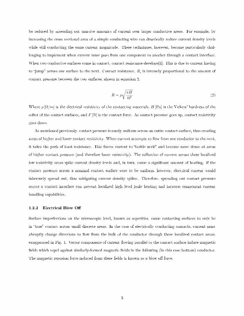
Surface imperfections on the microscopic level, known as asperities, cause contacting surfaces to only be

in �true� contact across small discrete areas. In the case of electrically conducting contacts, current must

abruptly change directions to �ow from the bulk of the conductor through these localized contact areas,

exaggerated in Fig. 1. Vector components of current �owing parallel to the contact surface induce magnetic

�elds which repel against similarly-formed magnetic �elds in the following (in this case bottom) conductor.

The magnetic repusion force induced from these �elds is known as a blow o� force.

3

Figure 1: Current �owing through contacting asperities (2D Side View)

This blow o� force e�ectively tries to separate the contacting bodies as current passes across the contact

interface. A clamping force is therefore required provide the necessary contact pressure to prevent separation

at current start up. The magnitude of blow o� force is proportional to current squared and depends on surface

geometry. In the simple case of two single point butt contacts, the blow o� force to current relationship

is shown in equation 3[2]. Localized contact pressure therefore creates areas of higher and lower contact

resistivity. When current attempts to �ow from one conductor to the next, it takes the path of least

resistance. This forces current to �bottle neck� and become more dense at areas of higher contact pressure

(and therefore lower resistivity). The collection of current across these localized low-resistivity areas spike

current density levels and, in turn, require a signi�cant amount of clamping force, Fs [N], to prevent electrical

blowo�.

Fs = 4.45e−7 N/A2 ∗ I2 (3)

The current squared relationship causes high levels of current to produce signi�cant blow o� force.

Inadequate contact pressure can result in electrical blow o� and lead to dangerous and even catastrophic

system failures. To prevent large blow o� forces from developing, the amount of current �owing through a

given area of contact must be reduced, or the amount of contact area current is �owing through must increase.

In many cases, reducing current also reduces system capabilities and physical or geometric constraints prevent

a signi�cant increase in contact area. In these situations, a method to increase contact area without changing

the overall size or shape of the contacting conductors would be very bene�cial. While surface asperities will

still exist, spread out contact pressure will result in more �true� contact points than localized contact pressure

and therefore reduce blow o� magnitudes.

4

1.3 Scope

The work done here analyzes the feasibility of the Predicted Displacement Method, a novel tool proposed

to design and control contact interfaces. This work presents a �rst-glance look at its performance. The

objective of this method is to spread out contact pressure across an entire nominal contact surface area. The

scope is limited to static 2-Dimensional simulations that model real-world contact situations. In order to

determine if further investigation of this idea is warranted, a proof of concept and two applications of this

idea are presented. The proof of concept consists of applying this method to a simple cantilevered beam

example. This method is then later applied to contacting disk and plate assemblies. The simulations used to

analyze this idea are are fundamental solid-mechanics based FEA codes that include a nonlinear simultaneous

contact solver. The simulations focus on comparing contact pressure results of classically shaped contact

surfaces to the altered designed shape derived from the Predicted Displacement Method. Friction, wear,

tribology, micro asperities, and dynamic e�ects are not included in this investigation.

2 Literature Review

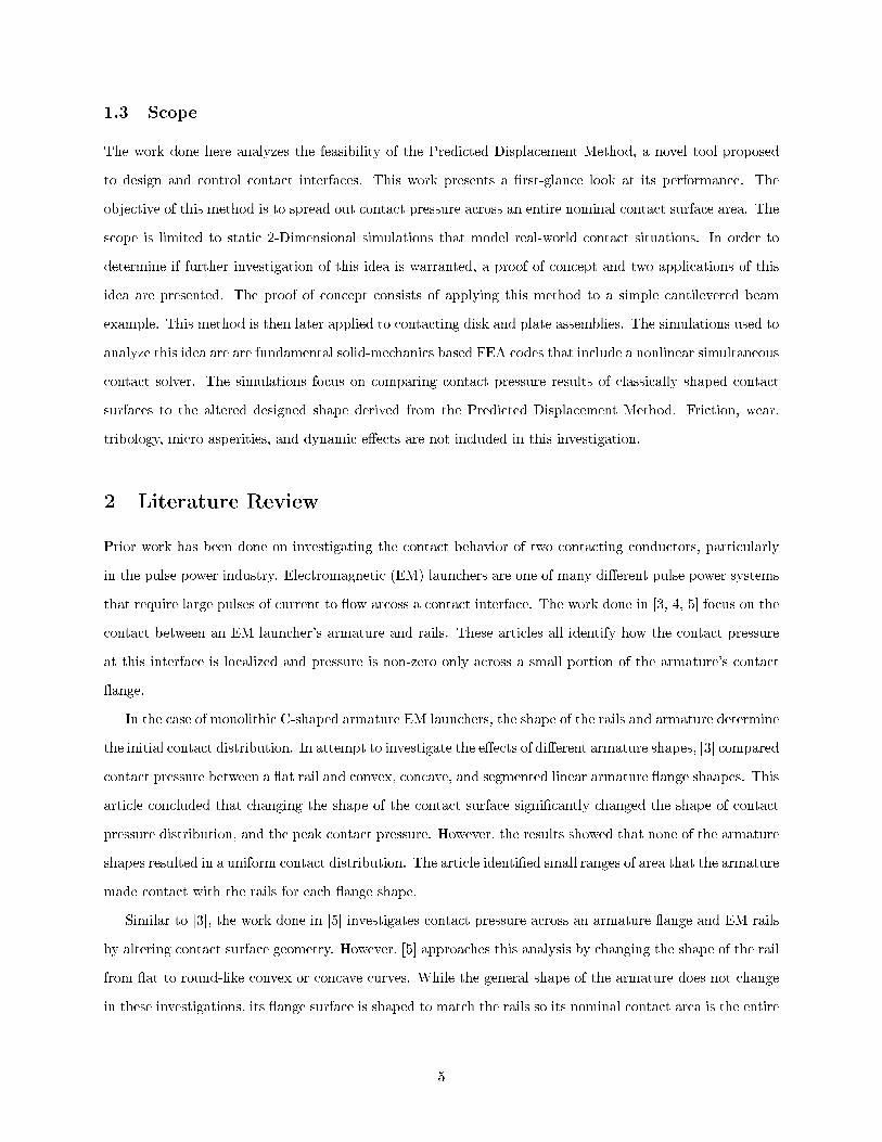
Prior work has been done on investigating the contact behavior of two contacting conductors, particularly

in the pulse power industry. Electromagnetic (EM) launchers are one of many di�erent pulse power systems

that require large pulses of current to �ow arcoss a contact interface. The work done in [3, 4, 5] focus on the

contact between an EM launcher's armature and rails. These articles all identify how the contact pressure

at this interface is localized and pressure is non-zero only across a small portion of the armature's contact

�ange.

In the case of monolithic C-shaped armature EM launchers, the shape of the rails and armature determine

the initial contact distribution. In attempt to investigate the e�ects of di�erent armature shapes, [3] compared

contact pressure between a �at rail and convex, concave, and segmented linear armature �ange shaapes. This

article concluded that changing the shape of the contact surface signi�cantly changed the shape of contact

pressure distribution, and the peak contact pressure. However, the results showed that none of the armature

shapes resulted in a uniform contact distribution. The article identi�ed small ranges of area that the armature

made contact with the rails for each �ange shape.

Similar to [3], the work done in [5] investigates contact pressure across an armature �ange and EM rails

by altering contact surface geometry. However, [5] approaches this analysis by changing the shape of the rail

from �at to round-like convex or concave curves. While the general shape of the armature does not change

in these investigations, its �ange surface is shaped to match the rails so its nominal contact area is the entire

5

top surface, similar to a straight edge �ange. Additionally, [5] investigates the e�ect of slits, or small gaps, in

armature �anges on contact pressure distribution. Rather than a solid �ange, a line is cut into the armature

�ange in the direction of the rails. The results of this work show that the change of rail shape directly e�ects

the contact pressure distribution. The location, size, and magnitude of contact area all change depending on

the rail curvature. However, the resulting distributions remain localized and only cover a small portion of

the armature �ange. The results of the split-leg armature simulations show that the area of contact remains

roughly the same, but the locations of peak contact pressure are changed. The split in the armature �ange

produces peak contact pressures at the edges of the splits. Where as a non-split armature has contact peaks

on its outside edges. As a whole, the results shown in [5] suggest methods of controlling locations of peak

contact pressures, but a method to spread out this pressure is still desired.

The results presented in these articles provided a basis to the fundamental concept introduced in this

paper. It was shown that changing the shape of the contact surfaces signi�cantly e�ected the contact pressure

distribution. Rather than investigating contact distributions at discrete particular shapes of contact surfaces,

a method that solves for the best shape would be advantageous. Developing a method to �nd the perfect

shape would provide a means to create uniform contact distributions across any surface, rather than for only

a speci�c situation.

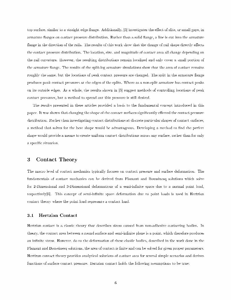
3 Contact Theory

The macro level of contact mechanics typically focuses on contact pressure and surface deformation. The

fundamentals of contact mechanics can be derived from Flamant and Boussinesq solutions which solve

for 2-Dimensional and 3-Dimensional deformations of a semi-in�nite space due to a normal point load,

respectively[6]. This concept of semi-in�nite space deformation due to point loads is used in Hertzian

contact theory where the point load represents a contact load.

3.1 Hertzian Contact

Hertzian contact is a classic theory that describes stress caused from non-adhesive contacting bodies. In

theory, the contact area between a round surface and semi-in�nite plane is a point, which therefore produces

an in�nite stress. However, do to the deformation of these elastic bodies, described in the work done in the

Flamant and Boussinesq solutions, the area of contact is �nite and can be solved for given proper parameters.

Hertizan contact theory provides analytical solutions of contact area for several simple scenarios and derives

functions of surface contact pressure. Hertzian contact holds the following assumptions to be true:

6

1. The strains are small and within the elastic region.

2. The area of contact is much smaller than the size of the body, allowing each body to be considered an

elastic semi-in�nite space

3. The surfaces are continuous

4. Frictionless / non-adhesive contact

Classic solutions provided by Hertzian contact theory include analytical contact pressure solutions for several

simple shape cases such as: sphere and sphere contact, cylinder and half-space contact, conical and half-

space, etc. The solutions for these examples are readily found and commonly used in speci�cally related

situations such as mechanical bearing or gear contacts.[7] These convenient analytical solutions are limited to

the several common contact cases encompassed within Hertzian theory. Because the Predicted Displacement

Method aims to normalize contact pressure across any two surfaces, it reaches beyond the scope of Hertzian

contact theory.

3.2 Computational Contact Mechanics

A more general approach to solving for contact pressure utilizes energy methods and numerical solvers. The

potential energy within a particular body, Π, changes upon deformation of the body. When two bodies

statically contact one another, their opposing deformations �nd an equilibrium and contact pressure, or

gaps, develops between them. This equilibrium point is where the total potential energy in the system is

minimized within conditional constraints. This section introduces the methods used to solve for contact

pressure via Finite Element Analysis (FEA) in this work. The complexity of computational contact solvers

makes simple examples the most convenient method of description. The following sections walk through a

simple mass-spring example that is a commonly used approach of introducing the solution of computational

contact mechanics. This example is taken from [8].

3.2.1 Model Formulation

In this simple contact example, a point mass of mass m [kg] is supported by a spring with sti�ness k [N/m].

Its de�ection u [m], is limited by by a rigid plane, or ��oor�, of distance h [m] below its non-de�ected height,

seen in Fig. 2. A model is desired that allows the calculation of u. The energy method is employed and a

variational approach to solving it is required. The potential energy for this system can be written as equation

4.

7

Figure 2: Mass spring system

Π(u) =1

2ku2 −mgu (4)

If there were no restriction on the mass's displacement, u, caused by the ��oor�, the minimum potential

energy of the system can quickly be solved by setting its derivative equal to zero. Using numerical solvers,

the derivative is solved by means of variation of the dependent variable u, leading to equation 5 that yields

u = mgk .

δΠ(u) = kuδu−mgδu = 0 (5)

Because the mass is unable to penetrate the �oor, the clearance between the mass and �oor, c [m], must not

be negative and therefore:

c(u) = h− u ≥ 0 (6)

If the mass makes contact with the �oor, c(u) = 0, then a reaction force appears. This reaction force, de�ned

here as FR [N], must be compressive and therefore of negative magnitude.

FR ≤ 0 (7)

Two possible cases are possible in this example. The �rst, the spring sti�ness is large enough to prevent

the mass from contacting the �oor. In which case the conditions c(u) > 0 and FR = 0 hold. Second, the

mass contacts the �oor where c(u) = 0 and FR < 0. These statements can be combined into what is known

as a Hertz-Signorini-Moreau condition, shown below.

c(u) ≥ 0 , FR ≤ 0 and FRc(u) = 0 (8)

8

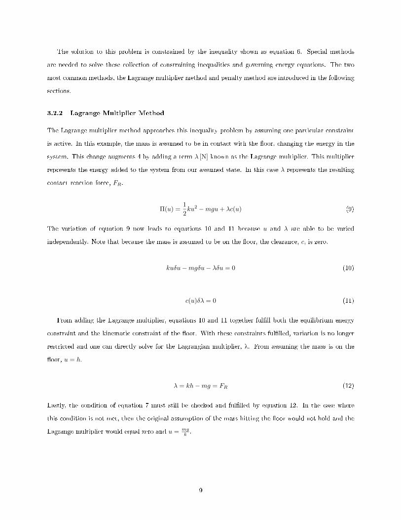
The solution to this problem is constrained by the inequality shown as equation 6. Special methods

are needed to solve these collection of constraining inequalities and governing energy equations. The two

most common methods, the Lagrange multiplier method and penalty method are introduced in the following

sections.

3.2.2 Lagrange Multiplier Method

The Lagrange multiplier method approaches this inequality problem by assuming one particular constraint

is active. In this example, the mass is assumed to be in contact with the �oor, changing the energy in the

system. This change augments 4 by adding a term λ [N] known as the Lagrange multiplier. This multiplier

represents the energy added to the system from our assumed state. In this case λ represents the resulting

contact reaction force, FR.

Π(u) =1

2ku2 −mgu+ λc(u) (9)

The variation of equation 9 now leads to equations 10 and 11 because u and λ are able to be varied

independently. Note that because the mass is assumed to be on the �oor, the clearance, c, is zero.

kuδu−mgδu− λδu = 0 (10)

c(u)δλ = 0 (11)

From adding the Lagrange multiplier, equations 10 and 11 together ful�ll both the equilibrium energy

constraint and the kinematic constraint of the �oor. With these constraints ful�lled, variation is no longer

restricted and one can directly solve for the Lagrangian multiplier, λ. From assuming the mass is on the

�oor, u = h.

λ = kh−mg = FR (12)

Lastly, the condition of equation 7 must still be checked and ful�lled by equation 12. In the case where

this condition is not met, then the original assumption of the mass hitting the �oor would not hold and the

Lagrange multiplier would equal zero and u = mgk .

9

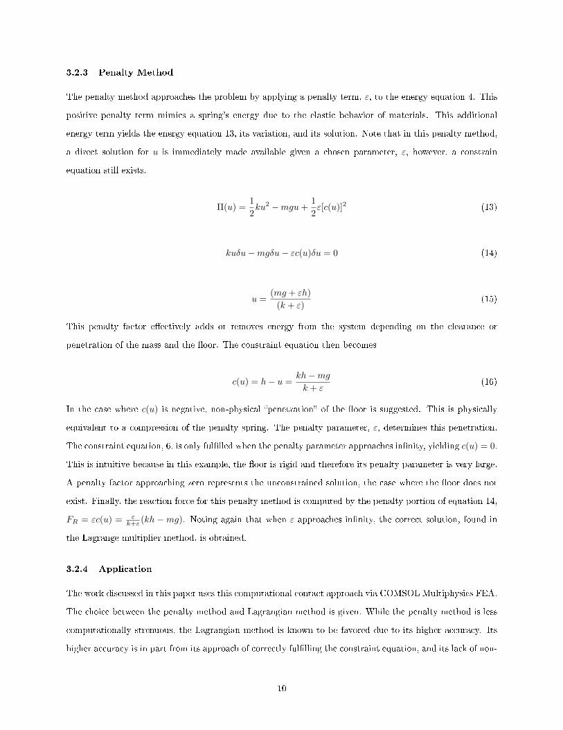
3.2.3 Penalty Method

The penalty method approaches the problem by applying a penalty term, ε, to the energy equation 4. This

positive penalty term mimics a spring's energy due to the elastic behavior of materials. This additional

energy term yields the energy equation 13, its variation, and its solution. Note that in this penalty method,

a direct solution for u is immediately made available given a chosen parameter, ε, however, a constrain

equation still exists.

Π(u) =1

2ku2 −mgu+

1

2ε[c(u)]2 (13)

kuδu−mgδu− εc(u)δu = 0 (14)

u =(mg + εh)

(k + ε)(15)

This penalty factor e�ectively adds or removes energy from the system depending on the clearance or

penetration of the mass and the �oor. The constraint equation then becomes

c(u) = h− u =kh−mgk + ε

(16)

In the case where c(u) is negative, non-physical �penetration� of the �oor is suggested. This is physically

equivalent to a compression of the penalty spring. The penalty parameter, ε, determines this penetration.

The constraint equation, 6, is only ful�lled when the penalty parameter approaches in�nity, yielding c(u) = 0.

This is intuitive because in this example, the �oor is rigid and therefore its penalty parameter is very large.

A penalty factor approaching zero represents the unconstrained solution, the case where the �oor does not

exist. Finally, the reaction force for this penalty method is computed by the penalty portion of equation 14,

FR = εc(u) = εk+ε (kh −mg). Noting again that when ε approaches in�nity, the correct solution, found in

the Lagrange multiplier method, is obtained.

3.2.4 Application

The work discussed in this paper uses this computational contact approach via COMSOL Multiphysics FEA.

The choice between the penalty method and Lagrangian method is given. While the penalty method is less

computationally strenuous, the Lagrangian method is known to be favored due to its higher accuracy. Its

higher accuracy is in part from its approach of correctly ful�lling the constraint equation, and its lack of non-

10

physical penetrations.[8] COMSOL's Lagrangian method was chosen for all contact simulations presented in

this work. To verify its reliability, initial contact results were compared to a di�erent contact solver provided

in the program Abaqus to ensure congruence.

4 Predicted Displacement Method

The Predicted Displacement Method (PDM) is designed to provide engineers a speci�c contact surface

shape for a given contact body that when loaded to a designed contact pressure, results in a uniform contact

pressure distribution. This method requires the user to input both contacting body's geometry, material,

loading conditions, and applicable constraints. With this information, the user can use FEA packages

to simulate each contacting body's response to a uniform boundary load. The PDM utilizes the identical

response to a uniform boundary load and uniform contact pressure load of an isotropic linear elastic material.

Both displacement responses of the contacting bodies to the uniform load can be superimposed and used to

re-shape one of the bodies, leaving the other as is. The re-shaping of the body and its contact surface now

accounts for the response of a designed-for uniform contact pressure acting on on both surfaces.

The PDM also utilizes identical responses to identical loads of di�erent shaped bodies with the same

section modulus. In other words, a straight cantilevered beam with a rectangular cross section of 1�x1� will

have the exact same response to a particular load as a similar 1�x1� cantilevered rectangular beam that is

curved or sloped rather than straight. This example is illustrated in Fig. 3.

Figure 3: De�ection comparison between beams in bending. Straight beam (top) de�ects same as non-straight beam (bottom)

This phenomenon allows the re-shaping of a contact body without compromising its predicted response

11

to a speci�ed load. After the slight alteration of geometry, once the contacting bodies are pressed together,

the alteration of shape accounts for the de�ection of both bodies and results in a uniform contact pressure

distribution. Methodology, theory, and proof for this method are discussed in the following subsections.

4.1 Theory

The PDM is built upon several di�erent engineering and mathematical principals. Continuum mechanics,

elastic theory, material mechanics, and two dimensional beam theory are the main foundations for the

feasibility of the PDM. This method also employs the ability to mimic uniform contact pressure with a

uniform boundary load in FEA simulations.

4.1.1 Assumptions

The Predicted Displacement Method assumes the contacting bodies are homogeneous isotropic materials

that behave in the linear elastic region. While theory and preliminary simulations suggest this method is

applicable to for plasticity behaving and soft materials, further work must be conducted to support these

suggestions. This method also assumes microscopic imperfections, such as asperities, microscopic cracks etc.,

are relatively uniform across the contacting surfaces and have negligible e�ects on resulting contact pressure.

Lastly, this process assumes the surface deformation due to contact, and total bodily de�ection, is much

smaller than the nominal size of the body.

4.1.2 Linear Elastic Behavior

In the �eld of engineering, it is known that a one dimensional spring changes in length by a linearly propor-

tional amount of the load placed on it. The mathematical model of this relationship is known as Hooke's

Law and is shown as equation 17, where F [N] is the force applied to the spring, x [m] is the change in length

of the spring, and k [N/m] is the spring constant.

F = kx (17)

Linear elastic material behaves in a similar manner. For materials, the linear relationship between force and

displacement is more commonly represented by another form of Hooke's Law, shown as equation 18, where

σ [Pa] represents stress, ε [m/m] represents strain, and E [Pa] is the material's modulus of elasticity.

σ = Eε (18)

12

In three dimensional space, the single variables of Hooke's Law are replaced with vectors or tensors. With

respect to an arbitrary Cartesian coordinate system, the relationship between force and displacement be-

comes:

F1

F2

F3

=

k11 k12 k13

k21 k22 k23

k31 k32 k33

X1

X2

X3

(19)

The 3x3 matrix is known as a sti�ness tensor which when inverted, becomes the material's compliance

matrix. This allows one to solve for deformation given an applied force, or, solve for reaction force given a

displacement. The linear relationship causes negative forces to produce negative displacements or negative

set displacements to cause opposite reaction forces. The PDM is able to utilize these features by applying

negative pressures to bodies and record the reaction. Then, by altering the body's geometry to account for

this �negative� reaction, a set displacement forcing the altered geometry back to its original shape will result

in the original reaction force �rst loaded on the unaltered body. This is made more clear with the following

uni-axial load example.

A cylindrical bar is to be placed in contact with a rigid semi-in�nite space with a designed contact load

P . A load F , which represents the opposite of the desired �nal contact load P , is applied to the bar to cause

a displacement of ∆x. The bar with original length l is then altered to account for the change in length.

The new bar, with a length of l +Δx, is then pressed against the rigid surface until the bar deforms by an

amount of Δx. So long as the de�ection Δx is much smaller than the original length l, then the resulting

reaction force will be very close to the design value, F . The resulting contact pressure between the rigid

surface and cylindrical bar will therefore be almost identical to the nominal design contact load, P . Fig. 4

depicts this example.

The relationship between the axial force placed on the bar and its resulting displacement is described as

equation 17. In the case of axially loaded elastic bodies, the sti�ness, k [N/m], is calculated with equation

20, where A [m2] is the cross sectional area of the bar, and and L [m] is the bar's nominal length.

k =AE

L(20)

13

Figure 4: Comparison between axial de�ection from load and reaction force from forced de�ection

This behavior is extrapolated by the PDM and applied to object surfaces. Each element of the contact

surface behaves in a similar manner to axial loads and allows contact surface pressure to be readily controlled

in the component design phase.

4.1.3 Euler-Bernoulli Beam De�ection

Euler-Bernoulli beam theory was used as another building block for the PDM to account for contact loads

causing bending stresses in contact bodies. The principal behavior utilized in this theory is the beam

de�ection's dependence on the cross sectional second moment of area, I, and not its extrusion path in the x

direction, as suggested previously in Fig. 3. The mathematical support for this phenomenon is derived from

the Euler-Bernoulli relationship between homogeneous beam displacement, y(x), and a distributed load,

w(x). This is shown as equation 21.

EId4y

dx4= −w(x) (21)

To solve for beam displacement, equation 21 is integrated four times. When integrated, beam displace-

ment, w(x) becomes shear force, V (x), which when integrated again becomes moment, M(x). The constants

of integration are accounted for by applying the applicable boundary conditions to the integration bounds.

In the case of a cantilevered beam of length l, the boundary conditions are y0 = 0, Vl = 0, Ml = 0, and

θ0 = 0, where θ = dydx . The resulting relationship is the common cantilevered beam de�ection under uniform

14

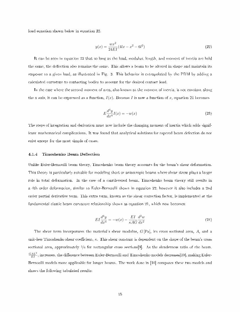
load equation shown below in equation 22.

y(x) =wx2

24EI(4lx− x2 − 6l2) (22)

It can be seen in equation 22 that so long as the load, modulus, length, and moment of inertia are held

the same, the de�ection also remains the same. This allows a beam to be altered in shape and maintain its

response to a given load, as illustrated in Fig. 3. This behavior is extrapolated by the PDM by adding a

calculated curvature to contacting bodies to account for the desired contact load.

In the case where the second moment of area, also known as the moment of inertia, is not constant along

the x-axis, it can be expressed as a function, I(x). Because I is now a function of x, equation 21 becomes

Ed4y

dx4I(x) = −w(x) (23)

The steps of integration and derivation must now include the changing moment of inertia which adds signif-

icant mathematical complications. It was found that analytical solutions for tapered beam defection do not

exist except for the most simple of cases.

4.1.4 Timoshenko Beam De�ection

Unlike Euler-Bernoulli beam theory, Timoshenko beam theory accounts for the beam's shear deformation.

This theory is particularly suitable for modeling short or anisotropic beams where shear stress plays a larger

role in total deformation. In the case of a cantilevered beam, Timoshenko beam theory still results in

a 4th order deformation, similar to Euler-Bernoulli shown in equation 22, however it also includes a 2nd

order partial derivative term. This extra term, known as the shear correction factor, is implemented at the

fundamental elastic beam curvature relationship shown as equation 21, which now becomes:

EId4y

dx4= −w(x)− EI

κAG

d2w

dx2(24)

The shear term incorporates the material's shear modulus, G [Pa], its cross sectional area, A, and a

unit-less Timoshenko shear coe�cient, κ. This shear constant is dependent on the shape of the beam's cross

sectional area, approximately 5/6 for rectangular cross sections[9]. As the slenderness ratio of the beam,

GAL2

EI , increases, the di�erence between Euler-Bernoulli and Timoshenko models decreases[10], making Euler-

Bernoulli models more applicable for longer beams. The work done in [10] compares these two models and

shows the following tabulated results:

15

Table 1: Euler and Timoshenko De�ection Comparison[10]

Slenderness Ratio Timoshenko De�ection / Euler De�ection

25 1.12050 1.060100 1.0301000 1.003

4.2 Analytical Approach

An analytical approach was taken to investigate the possibility of solving for a particular shape of a body that

yields uniform contact pressure when deformed by a known amount. A Euler-Bernoulli cantilevered beam

was chosen as the geometry for this approach due to its simplicity and well-known behavior and de�ection

relationships. This cantilevered beam is to be initially shaped by a function f(x) that is to be solved for in

this analytical approach. This initial shape, f(x), interferes with a rigid half-plane boundary and contact

pressure is induced when the uniform cross section curved beam de�ects under it.

Further simpli�cation of this analytical investigating is achieved by substituting uniform contact pressure

with a uniform load, w(x) = constant, and by assuming this uniform contact force is achieved when the

post-deformation beam is �at. In other words, a uniform load, w(x), is applied to a curved beam of shape

f(x), so that it de�ects to a perfectly �at, f(x) = 0, position. The governing equation for deriving this

beam's deformation is labeled as equation 21. Because this governing equation does not rely on beam shape,

but only moment of inertia, I, its de�ection under a uniform load has been previously derived under the

conditions of a cantilevered beam, shown as equation 22. This suggests that if the beam were to be shaped

so that its initial shape, f(x), were to equal its expected displacement under a uniform load, y(x), than

uniform contact could be achieved. However, this theory relies on several assumptions including no shear

e�ects, perfectly �xed cantilever boundary, and a rigid half-plane contact surface.

Because these assumptions do not hold in reality, a more accurate model is needed. Analytical solutions

of beam deformation increase in complexity as these assumptions are eliminated, and as geometry becomes

more complex. For example, the derivation of a Timoshenko modeled cantilevered beam under a point load

is shown in [11]. This lengthy and cumbersome process results in a deformation gradient that accounts for

shear e�ects in the beam, but promotes the use of numerical solvers to account for these realities.

4.2.1 Conclusions

In theory, if a beam is shaped the opposite of its expected de�ection from a given load, such load will deform

it back to its ��at� state. Analytical solutions are limited by mathematical complexities in deformation

gradients and their relationships with given loads. For example, an analytical deformation solution for

16

a Timoshenko cantilevered beam undergoing a end-point load may exist, but an analytical solutions for

complex or discontinuous loads may not. Numerical solutions, such as FEA, can be used to provide these

deformation solutions for any load case. It was quickly concluded that trying to �nd the beam shape that

results in uniform contact would be done via. numerical solvers.

4.3 Methodology

The application of the PDM method begins by constructing a model for an independent contact body. The

body is to be shaped in a manner that does not promote contact with another body. In other words, the model

should incorporate the body's nominal shape, before any augmentations were made to induce contact (such

as shaping for interference �ts). A solid mechanics simulation is then developed with boundary conditions

that mimic the body's real world constraints and non-contact loads. At this point, the �nal desired contact

pressure is added into the simulation as a negative (opposite direction) uniform boundary load.

Post processing of this simulation will yield the body's response to this negative �contact� load. The next

step in the PDM is to apply this displacement response of the body onto its original shape. Speci�cally, the

shape of the deformed body under the negative contact load becomes the body's new shape. The amount

of re-shaping applied to the body has negligible e�ects to its structural integrity and physical behavior.

Additionally, the body will be pressed back to its original shape once the true contact load is applied. This

process is then repeated with the second body.

New models are then created with the newly shaped contacts. A new simulation is then created, incor-

porating both bodies and de�ning contact between them. When pressed to the designed contact load, the

resulting contact pressure exempli�es the uniform load placed on the individual bodies.

Alternatively, it is possible to incorporate both body's displacement responses onto only one of the bodies.

The re-shaping of one of the contacts can account for the displacement of both under a designed load. The

methodology described remains the same, however, the response of the second body is applied to the �rst

body in addition to its own response. This process allows one of the bodies to remain unchanged and can

save time and money when used in application. When doing this, it is important that displacement vector

directions and material are considered.

4.4 Proof of Concept

The PDM's feasibility was tested on a simple cantilevered beam forced to contact a semi-in�nite elastic body

through geometry interference. A cantilevered beam was chosen for a proof of concept because of the ability

to derive analytical deformation solutions. Additionally, this cantilevered beam model o�ered simple design

17

and simulation abilities in regards to geometry de�nition, boundary condition applications, and meshing.

In order for contact pressure to develop through interference, the cantilevered beam must have an initial

displacement or shape that causes the beam to deform when forced past the other contacting body. The

goal of this experiment was to use the PDM to �nd the ideal shape of a uniform cross section cantilevered

beam so that its contact pressure was constant across its entire nominal contact surface.

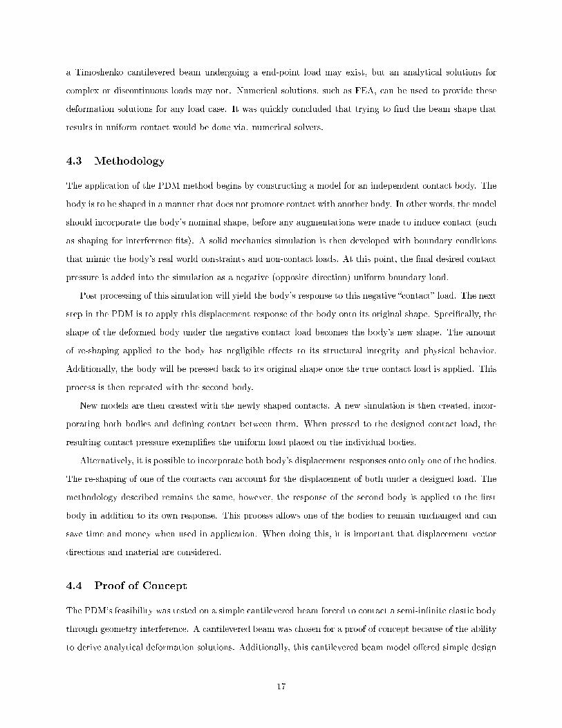
4.4.1 Model Setup

This experiment was designed to compare the resulting contact pressures of di�erent shaped cantilevered

beams. Each beam had a square cross section of 10mm in width and height through out its entire 100mm

length. This geometry results in a slenderness ratio of approximately 461. Table 1 suggests the use of a

Euler-Bernoulli beam model would be su�cient for this beam geometry. The beam's top surface is de�ned

as its nominal contact area and will be referred to as the slave, or destination, contact surface. The shape

of the beam is de�ned as the equation representing the curvature of the beam's neutral axis. Fig. 5 de�nes

the datum coordinate system along with an example beam that has a straight shape of y = −5.

Figure 5: Illustration of beam and establishment of coordinate system

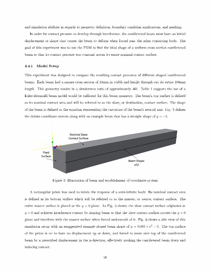
A rectangular prism was used to mimic the response of a semi-in�nite body. Its nominal contact area

is de�ned as its bottom surface which will be referred to as the master, or source, contact surface. The

entire master surface is placed at the y = 0 plane. As Fig. 5 shows, the slave contact surface originates at

y = 0 and achieves interference contact by shaping beam so that the slave contact surface crosses the y = 0

plane and interferes with the master surface when forced underneath of it. Fig. 6 shows a side view of this

simulation setup with an exaggerated example sloped beam shape of y = 0.001 ∗ x2 − 5. The top surface

of the prism is set to have no displacement up or down, and forced to move over top of the cantilevered

beam by a prescribed displacement in the x-direction, e�ectively pushing the cantilevered beam down and

inducing contact.

18

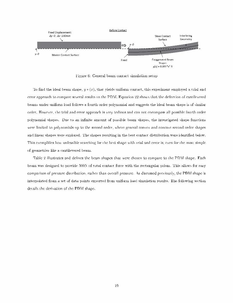
Figure 6: General beam contact simulation setup

To �nd the ideal beam shape, y ∗ (x), that yields uniform contact, this experiment employed a trial and

error approach to compare several results to the PDM. Equation 22 shows that the de�ection of cantilevered

beams under uniform load follows a fourth order polynomial and suggests the ideal beam shape is of similar

order. However, the trial and error approach is very tedious and can not encompass all possible fourth order

polynomial shapes. Due to an in�nite amount of possible beam shapes, the investigated shape functions

were limited to polynomials up to the second order, where general convex and concave second order shapes

and linear shapes were explored. The shapes resulting in the best contact distribution were identi�ed below.

This exempli�es how unfeasible searching for the best shape with trial and error is, even for the most simple

of geometries like a cantilevered beam.

Table 2 illustrates and de�nes the beam shapes that were chosen to compare to the PDM shape. Each

beam was designed to provide 500N of total contact force with the rectangular prism. This allows for easy

comparison of pressure distribution, rather than overall pressure. As discussed previously, the PDM shape is

interpolated from a set of data points exported from uniform load simulation results. The following section

details the derivation of the PDM shape.

19

Table 2: Beam curvature comparison

Curvature Equation Exaggerated Shape

Linear y = 0.0005x

Convex y = 5e−4x− 5e−6x2

Concave y = 5.35e−4x+ 1e−5x2

PDMLinearly connected data

points

To exemplify the sensitivity between the beam shape and the resulting contact pressure distribution, a

fourth order polynomial was derived from a least square curve �t of the PDM shape. This fourth order

polynomial, y = 3.545e−4x + 1.853e−4x2 − 1.190e−6x3 + 2.773e−9x4, was used as another beam shape to

compare to the discretized PDM beam. Fig. 7 shows the di�erence between the PDM shape and fourth

order shape with a residual plot. One can quickly notice that the fourth order beam shape closely �ts the

PDM shape within a few microns.

Figure 7: Residual of PDM shaped beam and 4th order curve �t of PDM shape

These linear, convex, concave, fourth order, and PDM beam shapes where then modeled and imported

into simulation software to solve for their respective contact pressures when forced into interference �t with a

20

rectangular elastic body. To investigate the feasibility of the PDM, their respective resulting contact pressure

is plotted against the x-axis of the slave contact surface and compared both qualitatively and quantitatively.

4.4.2 PDM Shape

As mentioned previously, the process of developing the PDM beam shape begins by analyzing each contact

body independently under a designed contact load. In this proof of concept, 500 newtons of contact force is

desired. A uniform boundary load of 500N was placed on each contact surface in the opposite direction of

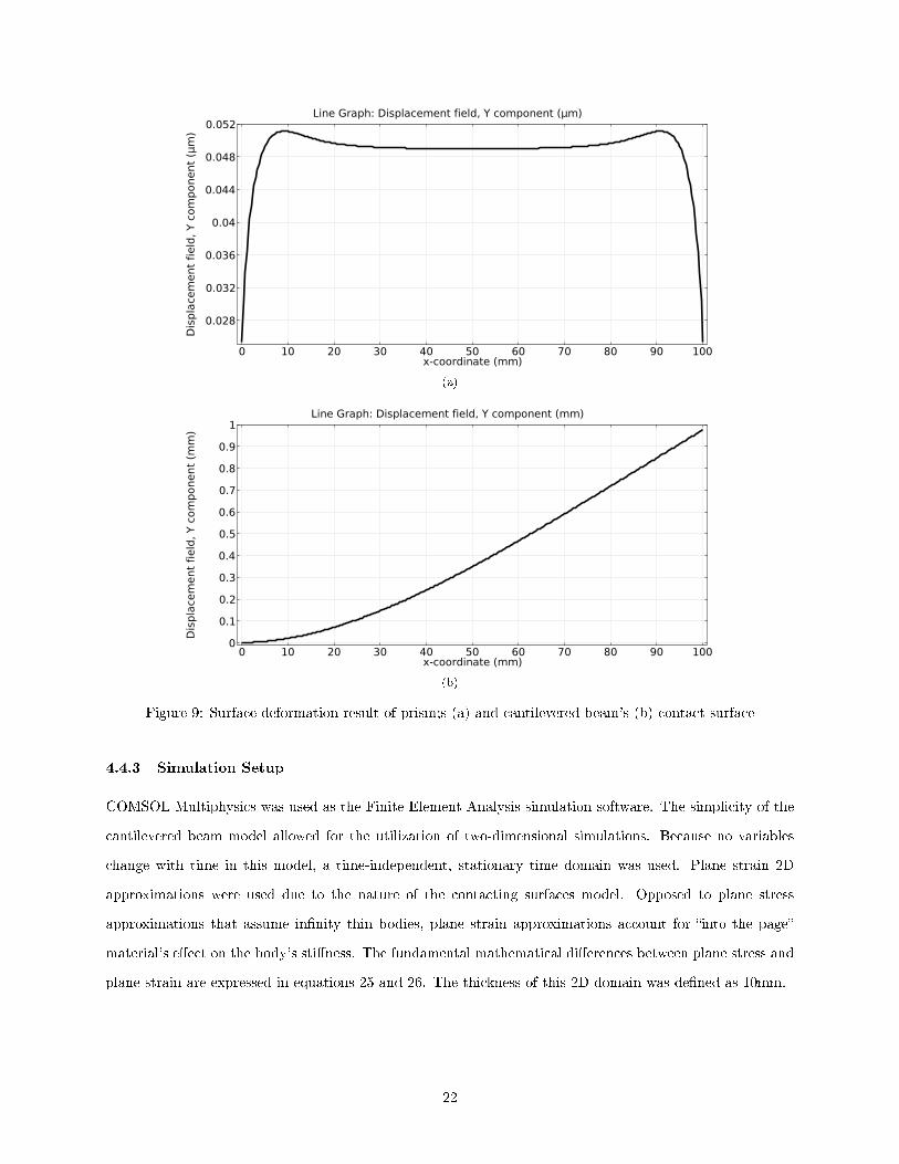
contact, as seen in Fig. 8. The resulting deformation of these surfaces, shown in Fig. 9, are then used to

create the PDM shape. In this case, the deformation plots were superimposed to create a total deformation

function dependent on x-axis location. This total deformation shape was used as the PDM beam's top

surface, and the same curve was shifted down 10mm to act as the PDM beam's bottom edge. Because of

the relatively small displacement values in the prism, seen in Fig. 9a, the PDM shape is best seen in Fig.

9b, the displacement of the cantilevered beam.

(a)

(b)

Figure 8: Visual representation of load on contact prism (a) and cantilevered beam (b)

21

(a)

(b)

Figure 9: Surface deformation result of prism;s (a) and cantilevered beam's (b) contact surface

4.4.3 Simulation Setup

COMSOL Multiphysics was used as the Finite Element Analysis simulation software. The simplicity of the

cantilevered beam model allowed for the utilization of two-dimensional simulations. Because no variables

change with time in this model, a time-independent, stationary time domain was used. Plane strain 2D

approximations were used due to the nature of the contacting surfaces model. Opposed to plane stress

approximations that assume in�nity thin bodies, plane strain approximations account for �into the page�

material's e�ect on the body's sti�ness. The fundamental mathematical di�erences between plane stress and

plane strain are expressed in equations 25 and 26. The thickness of this 2D domain was de�ned as 10mm.

22

PlaneStress

σz = 0

εz 6= 0

(25)

PlaneStrain

σz = ν(σx + σy)

εz = 0

(26)

The geometry used for simulation included two bodies, referred to as domains, where one represented

the cantilevered beam and the other representing the contact prism. The global coordinate system was

de�ned with length and angular units of millimeters and degrees, respectively. Both domains were assigned

to behave in a linear elastic manner, dependent on the material properties. Both domains were also assigned

initial conditions of zero displacement and velocity, u0 = dudt = 0.

The beam was shaped by de�ning the beam's top and bottom geometric edges as analytic functions

dependent on the spatial x-coordinate in the global coordinate system. Because of uniform rectangular cross

sections, the neutral axis of the beam is located in the geometric center which allowed the beam shape to

represent the top (contact) surface of the beam. To assist in post-processing data, the top left most corner

of the beam was placed at the global coordinate system datum, x = 0, y = 0. In doing this, the �rst point

of the beam shape coincided with the �rst point of the nominal contact surface. A �xed boundary condition

was applied to the base, left most, edge of the cantilevered beam. This �xed condition enforced zero x and

y displacements for all nodes on that edge, ux = uy = 0.

The rectangular prism was placed to the left of the cantilevered beam so that its bottom (contact) surface

was on the y = 0 line. To enforce semi-in�nite body like behavior, only the top surface of the prism was

constrained. Using a prescribed displacement boundary condition, the nodes on the top surface of the prism

could not displace in the y direction, and were forced to displace exactly 120mm in the x direction, ux = 120,

uy = 0. This boundary condition e�ectively acted as a �xed edge condition while forcing the prism to slide

over the beam, causing interference with the shaped beam. This method of inducing contact required a

slight geometric change if the rectangular prism. To aid in solver convergence, the bottom right corner of

the prism was �lleted, preventing errors when contacting the �xed edge of the beam.

Contact was then de�ned between the source and destination boundaries as the bottom prism surface,

including the �llet surface, and the beam's top surface, respectively. The contact solver chosen was the

augmented Lagrangian solver with an initial contact pressure of 0, Tn = 0. Because this model is not

incorporating any wear or overlapping material e�ects, surface o�set distances for the source and boundary

were set to 0, doffset,d = doffset,s = 0. The coordinate system, geometry, and boundary conditions are

23

displayed in Fig. 10, below.

Figure 10: COMSOL beam contact geometry de�nitions

While theory suggests the PDM is independent of material, the properties used for proof of concept

resembled typical aluminum alloy, described in Table 3. This material was chosen due to aluminum's wide

spread use in industry for eletrco-mechanical systems. Due to the fundamentals of linear elastic behavior, a

more sti� or compliant material choice would result in the exact same contact pressure distribution with a

linearly scaled magnitude.

Table 3: Material data of aluminum used in simulation

Property Value Units

Density 2700 kg/m3

Modulus of Elasticity 69e9 PaPoisson's Ratio 0.33 1

The meshing scheme chosen for this simulation utilized quadrilateral cell shapes for the shaped beam

and used triangular cell shapes for the prism with �llet. While the quadrilateral cell shapes are spatially

more e�cient, the accuracy of the result and length of computation have do not di�er from triangular cell

shaped meshes. Due to the computationally easy nature of 2D simulations, the mesh was able to be re�ned

to a size of 0.333mm. Care was taken to ensure no �bad� meshes were produced. This included checking for

long and narrow elements, convoluted distributions of mesh densities, rough edges, etc.

Fig. 11 shows the mesh result using a structured mesh for the beam and an unstructured mesh for

the prism. The discretization of the displacement �eld was set to quadratic, adding a degree of freedom

on element edges but allowing second order displacement between nodes. Each step of increasing the dis-

cretization order from linear, to higher orders such as quadratic, cubic, etc., add signi�cantly more degrees

of freedom which the solver must handle, and therefore increases computation time. Quadratic was chosen

because of the rapid diminishing returns in solution accuracy in exchange for computation time. For proper

completeness, simulation results have been compared with results of higher and lower levels of discretization

along with tighter and courser meshes. The meshing scheme illustrated in Fig. 11 represents a mesh level

that provides a high level of con�dence in result accuracy.

24

Figure 11: Meshing scheme used in beam contact simulations

The solver used for these studies was a Multifrontal Massively Parallel sparse direct Solver known as

MUMPS. This solver is the default solver for direct solution approaches in COMSOL. The two variables

solved for in these simulations are the displacement �eld, u, and contact pressure, Tn. A segregated approach,

opposed to fully coupled, was used because of contact pressure's dependence on the displacement �eld. A

fully coupled solver starts from an initial guess and applies Newton-Raphson iterations until the solution

has converged, while the segregated solver solves each physics sequentially until convergence. Simply put,

the solver solves for displacement and uses those results to then solve for contact pressure and iteratively

repeats these steps until convergence. The segregated solver also provides convergence plots for each physics

(in this case displacement �eld and contact pressure) and gives the user more insight while monitoring the

convergence. These results are then able to be post processed to display a wide variety of information such

as stress states, reaction forces, energy, etc.

4.4.4 Results

The prescribed displacement of the contact prism resulted in cantilevered beam displacement, as designed.

Fig. 12a shows the linear beam deformed under the prism, while plotting the resulting Von Mises stresses

in the bodies. The stress distribution is not typical of a cantilevered beam under uniform or end load,

suggesting the beam's contact with the prism is local towards the �xed end.

25

Figure 12: Von Mises stress plot of linear shaped beam in contact with prism

Figure 13: Zoomed-in view of labeled area in Fig. 12

Figure 14: Von Mises stress plot of PDM shaped beam in contact with prism

The PDM beam developed a much more typical cantilevered beam stress distribution, as seen in Fig.

14. Additionally, no visible gaps between the deformed beam and prism were found. To better analyze the

26

feasibility of the PDM, contact pressure across the slave contact surface must be evaluated both qualitatively

and quantitatively. Post processing of simulation results allow contact pressure to be plotted against the

x-direction of the beam's contact surface. The shape of this plot qualitatively shows how spread out the

contact pressure is. The goal of the PDM is to achieve a spread out, uniform contact pressure, opposed

to localized spikes of contact. The PDM shape was designed to provide a total contact force of 500N. To

quantitatively evaluate the resulting contact, the contact pressure plot is integrated twice, with respect to x

and z directions. Integrating contact pressure [N/m2] with respect to x results in line loads in the z direction

(into the page) as [N/m]. Due to the 2D nature of the simulation, the integration in the z direction involves

multiplying the line contact load by the model thickness, 10mm, resulting in total contact force in Newtons,

[N ].

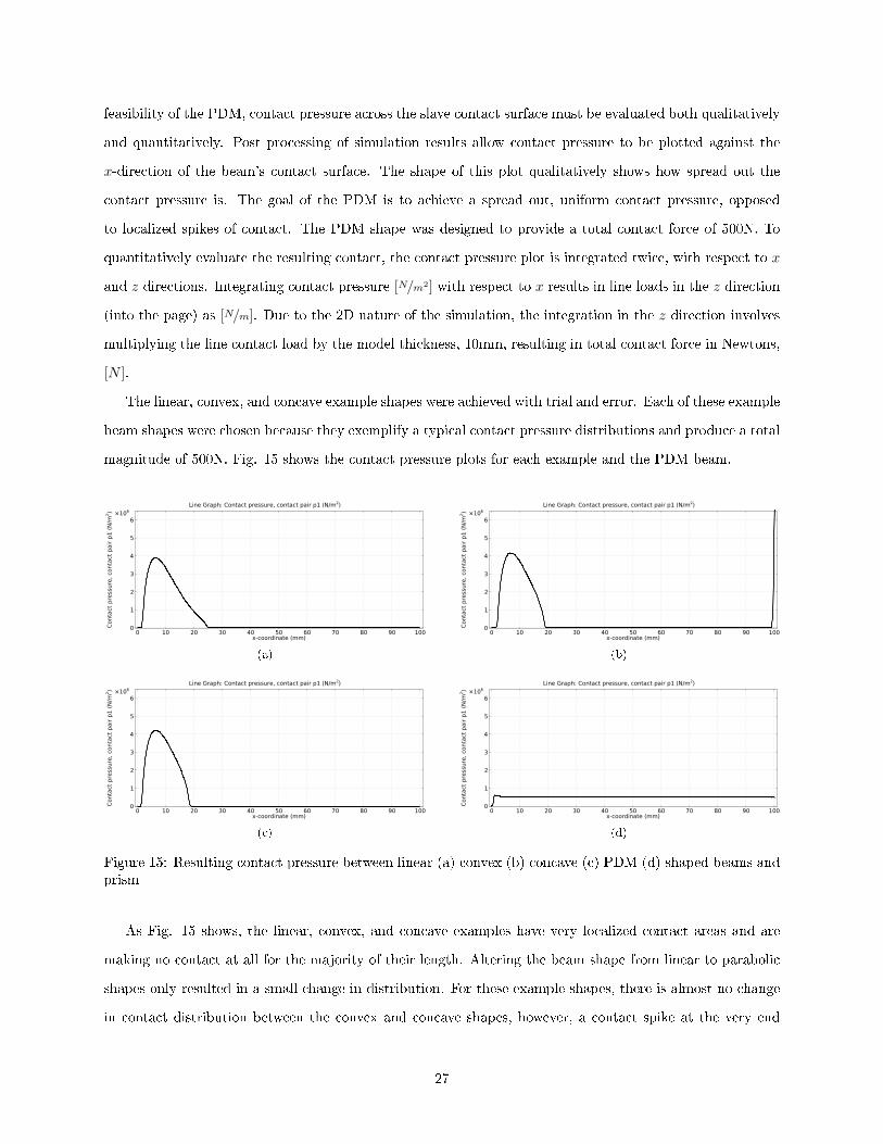
The linear, convex, and concave example shapes were achieved with trial and error. Each of these example

beam shapes were chosen because they exemplify a typical contact pressure distributions and produce a total

magnitude of 500N. Fig. 15 shows the contact pressure plots for each example and the PDM beam.

(a) (b)

(c) (d)

Figure 15: Resulting contact pressure between linear (a) convex (b) concave (c) PDM (d) shaped beams andprism

As Fig. 15 shows, the linear, convex, and concave examples have very localized contact areas and are

making no contact at all for the majority of their length. Altering the beam shape from linear to parabolic

shapes only resulted in a small change in distribution. For these example shapes, there is almost no change

in contact distribution between the convex and concave shapes, however, a contact spike at the very end

27

of the beam can be seen from the convex shape, Fig. 15b. While the convex shape did achieve multiple

points of contact, the total area of contact was only about 20% of the beam's nominal contact area. The

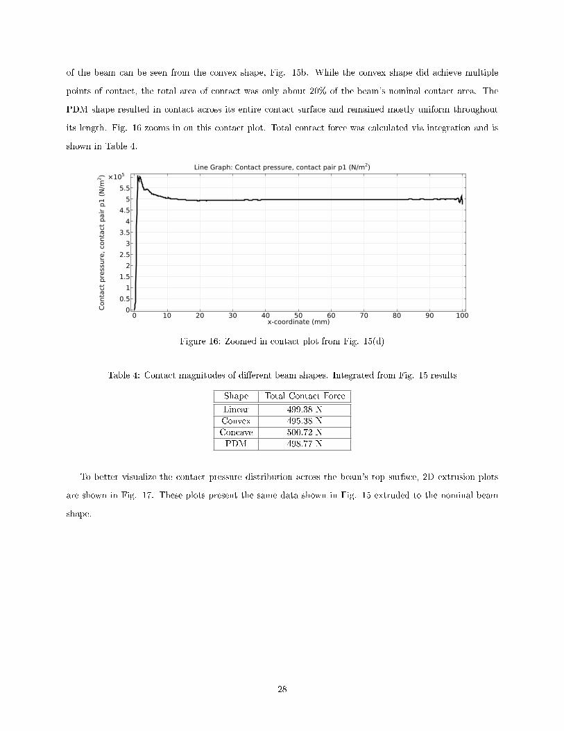
PDM shape resulted in contact across its entire contact surface and remained mostly uniform throughout

its length. Fig. 16 zooms in on this contact plot. Total contact force was calculated via integration and is

shown in Table 4.

Figure 16: Zoomed in contact plot from Fig. 15(d)

Table 4: Contact magnitudes of di�erent beam shapes. Integrated from Fig. 15 results

Shape Total Contact Force

Linear 499.38 NConvex 495.38 NConcave 500.72 NPDM 498.77 N

To better visualize the contact pressure distribution across the beam's top surface, 2D extrusion plots

are shown in Fig. 17. These plots present the same data shown in Fig. 15 extruded to the nominal beam

shape.

28

(a) (b)

(c) (d)

Figure 17: Extruded contact results displayed in Fig. 15

It was also found that the location and magnitude of contact on the beam could be altered by adjusting

the slope and initial displacement of the example shapes, but the contact distribution shape remains the

same. For example, Fig. # shows the contact distribution of a linearly sloped beam, similar to the previous

example, but with a di�erent slope and initial displacement, y = 0.003x − 2.0e−5. One can see how the

magnitude of contact changed, a total of 617N , but its distribution shape remained the same as seen in Fig.

15a. Fig. 18 also shows how the same contact distribution was in a di�erent location, further down the beam,

suggesting easy control of contact location and magnitude, but lack of control over contact distribution with

out PDM.

29

Figure 18: Resulting contact pressure of di�erent linearly shaped beam

Similar techniques were used to investigate di�erent parabolic, and even cubic shapes. It quickly became

evident that systematically trying di�erent beam shapes provided no progress in improving the contact

pressure distribution. Because of the ideal contact result of the PDM beam shape, least square curve �tting

was used to approximate the PDM's descrete shape. A fourth order analytic function was derived from the

curve �tting and used as another beam shape to investigate its contact pressure result. This fourth order

function's residual to the PDM shape is shown in Fig. 7. Noting the micrometer magnitude of residual

provides the ability for a fundamental sensitivity analysis on the beam shape's e�ect on resulting contact.

Fig. 19 shows the contact pressure plot of the fourth order beam shape.

Figure 19: Resulting contact pressure from beam shaped as a 4th order PDM approximation

4.4.5 Conclusions

The comparison of stress distributions in �gures 12 and 14 suggested drastic di�erences in contact loads.

The non-bending-like stress distribution of the linear shaped beam in Fig. 12 suggested a contact load very

30

close to the �xed end of the beam. This loading type would result in higher shear and normal stresses, rather

than bending stresses seen in Fig. 14. Zooming in on the linear shape stress plot, Fig. 13 visually shows no

contact at the free end of the beam, also suggesting localized contact towards the �xed end.

The dependent variable contact pressure, Tn, was solved for every destination boundary element. In

these cases, these elements consisted of the top beam surface and their values could be plotted along their

distance down the x-axis of the beam. These plots, shown in Fig. 15, show the contact pressure across the

entire beam surface. As suggested, the contact of the linear shaped beam was localized at the left end of the

beam and had zero contact everywhere else. The second order shapes also had a similar contact pressure

distribution, however, the convex shape did have a second point of contact at its free end. Even with two

points of contact, the amount of area that was in contact with the prism was less than 20% of the nominal

contact surface. This is better seen in the extrusion plots shown in Fig. 17.

In attempt to alter or improve the contact result of the linearly shaped beam, di�erent linear beam shapes

were investigated. With only two parameters to control, slope and initial position, it was quickly found that

no combination of parameters resulted in a better contact distribution. The slope and initial position e�ected

the contact pressure's location along the beam and its magnitude, but not its distribution shape. Fig. 18

exempli�es this with the contact result of a di�erent linear beam shape. Comparing the two presented

contact results of the two linear shapes shows this change in contact location and magnitude and also shows

how the distribution remained the same. Di�erent second order shapes were similarly investigated. Now

with three parameters to adjust, identifying any patterns or trends proved di�cult. This tedious approach

to �nding better contact distributions quickly proved to be unfeasible.

The PDM shape resulted in almost perfect contact, as seen in Fig. 16. Not only was contact pressure

existent from end to end of the beam, but its magnitude was uniform. This result is exceptionally close to

the desired result and strongly supports the validity of the Predicted Displacement Method. Additionally,

the resulting contact magnitude of 498.77N came within less than half of a percent of the desired force

magnitude of 500N. The relative spikes of contact of the PDM result are not indicative of realistic contact

behavior. These sudden changes in pressure are attributed to the nature of the numerical solvers.

Assuming the PDM shape to be the ideal or perfect shape, a fourth order polynomial was derived from

least squares curve �tting. Its residual, shown in Fig. 7, illustrates how the fourth order shape matches the

PDM shape within 1.3 microns. Even with this high R2 value, the contact pressure was signi�cantly altered,

as seen in Fig. 19. Comparing this contact plot to the residual plot shows how the �positive� di�erence or

residual of shape led to two signi�cant local contact spikes. This result exempli�ed how sensitive the beam

shape is to its resulting contact pressure. This fourth order shape result also shows how second and third

order shapes are not capable of providing a better contact distribution in this example. Increasing the order

31

of polynomials for the PDM curve �t would eventually converge to the PDM result.

In conclusion, the PDM shaped beam produced a perfect contact pressure distribution that was within

0.5% of the design goal. This simulation result not only supported the feasibility of the PDM, but it also

supported its capability of meeting contact magnitude and distribution design goals with precision. However,

these results identi�ed the sti� sensitivity of the PDM. The overall success in this proof of concept lead to

further investigations of the PDM's uses and applications.

5 Applications and Results

5.1 Thin Cylinders

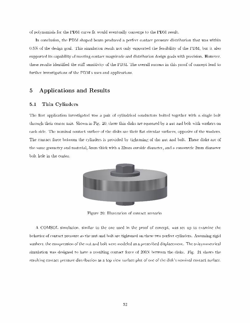
The �rst application investigated was a pair of cylindrical conductors bolted together with a single bolt

through their center axis. Shown in Fig. 20, these thin disks are squeezed by a nut and bolt with washers on

each side. The nominal contact surface of the disks are their �at circular surfaces, opposite of the washers.

The contact force between the cylinders is provided by tightening of the nut and bolt. These disks are of

the same geometry and material, 5mm thick with a 22mm outside diameter, and a concentric 2mm diameter

bolt hole in the center.

Figure 20: Illustration of contact scenario

A COMSOL simulation, similar to the one used in the proof of concept, was set up to examine the

behavior of contact pressure as the nut and bolt are tightened on these two perfect cylinders. Assuming rigid

washers, the compression of the nut and bolt were modeled as a prescribed displacement. The axisymmetrical

simulation was designed to have a resulting contact force of 200N between the disks. Fig. 21 shows the

resulting contact pressure distribution as a top view surface plot of one of the disk's nominal contact surface.

32

Figure 21: Axisymmetrical contact distribution simulation result of two perfect cylinders squeezed by con-centric nut, washer, bolt assembly

As one would expect, the contact pressure was concentrated towards the center of the disks, near the

bolt. The thin black circle displayed in this plot outlines the location of the washers. Fig. 21 also shows that

there is no contact at all towards the outer portions of the disk surface. This contact pressure distribution is

better examined from a 1-D plot of contact pressure vs. disk radius, r, shown in Fig. 22. In this application,

the nominal contact area is from r = 1 to r = 11.

Figure 22: Contact pressure in respect to disk radii along nominal contact surface

This plot, displaying the same data seen in the previous surface plot, shows more clearly how the contact

pressure is zero through out most of the nominal contact area. Not only is the contact pressure zero in

33

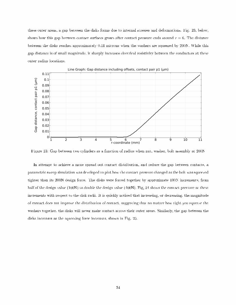
these outer areas, a gap between the disks forms due to internal stresses and deformations. Fig. 23, below,

shows how this gap between contact surfaces grows after contact pressure ends around r = 6. The distance

between the disks reaches approximately 0.11 microns when the washers are squeezed by 200N. While this

gap distance is of small magnitude, it sharply increases electrical resistivity between the conductors at these

outer radius locations.

Figure 23: Gap between two cylinders as a function of radius when nut, washer, bolt assembly at 200N

In attempt to achieve a more spread out contact distribution, and reduce the gap between contacts, a

parametric sweep simulation was developed to plot how the contact pressure changed as the bolt was squeezed

tighter than its 200N design force. The disks were forced together by approximate 100N increments, from

half of the design value (100N) to double the design value (400N). Fig, 24 shows the contact pressure at these

increments with respect to the disk radii. It is quickly noticed that increasing, or decreasing, the magnitude

of contact does not improve the distribution of contact, suggesting that no matter how tight you squeeze the

washers together, the disks will never make contact across their outer areas. Similarly, the gap between the

disks increases as the squeezing force increases, shown in Fig. 25.

34

Figure 24: Contact pressure at di�erent assembly loads

Figure 25: Gap between disks at di�erent assembly loads

The PDM was then applied to this application to investigate its e�ect on contact pressure distribution. As

detailed in the previous sections, a uniform load of the design magnitude, 200N, was independently applied

to both contact surfaces while the body was constrained with realistic boundary conditions that modeled

the nut, bolt, and washers. The deformation response of both disks were superimposed and added to one of

the disk's contact surface. This resulted in a perfect cylinder pressed against a non-perfect cylinder whose

shape encouraged contact across is outer radius areas. The magnitude of this geometry alteration is very

small and only seen with exaggerated pictures, such as Fig. 26, below.

35

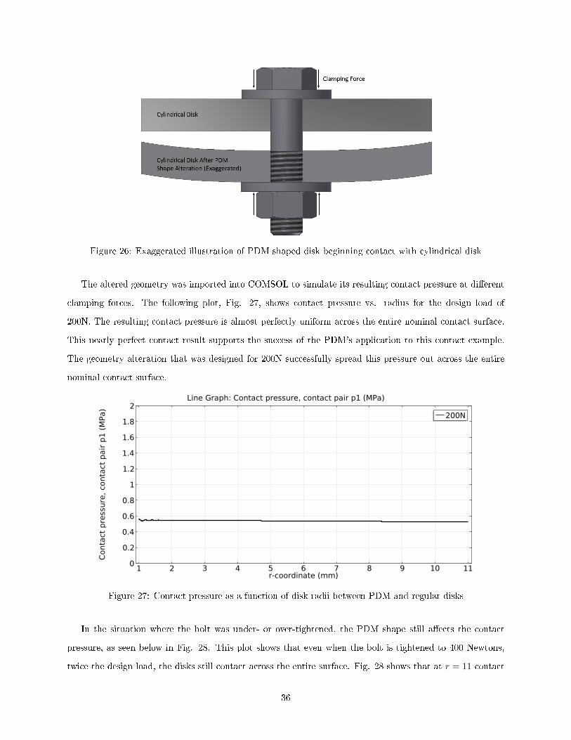
Figure 26: Exaggerated illustration of PDM shaped disk beginning contact with cylindrical disk

The altered geometry was imported into COMSOL to simulate its resulting contact pressure at di�erent

clamping forces. The following plot, Fig. 27, shows contact pressure vs. radius for the design load of

200N. The resulting contact pressure is almost perfectly uniform across the entire nominal contact surface.

This nearly perfect contact result supports the success of the PDM's application to this contact example.

The geometry alteration that was designed for 200N successfully spread this pressure out across the entire

nominal contact surface.

Figure 27: Contact pressure as a function of disk radii between PDM and regular disks

In the situation where the bolt was under- or over-tightened, the PDM shape still a�ects the contact

pressure, as seen below in Fig. 28. This plot shows that even when the bolt is tightened to 400 Newtons,

twice the design load, the disks still contact across the entire surface. Fig. 28 shows that at r = 11 contact

36

is non-zero for all cases of under and over tightening. Comparing this plot to the previous non-PDM perfect

cylindrical disk results, Fig. 24, indicates how the higher the clamping force is over the design load, the

closer it converges to the non-PDM contact shape.

Figure 28: Contact pressure results at di�erent assembly loads. Note ideal contact at design load andnon-zero contact at all loads contrasts Fig. 24 results

Fig. 28 also shows that when under-tightened, the contact pressure localizes where the PDM geometry

alteration promotes contact, towards the outer edge of the disks. This suggests there is a range of total

contact magnitude at which the PDM improves contact behavior. Within this magnitude range, perfect

contact is achieved when at the design load.

5.2 Prism and Plate Clamp

In this application of the PDM, a rectangular prism is squeezed by two plates through a bolted connec-

tion, shown in Fig. 29. This example will model this contact interface with a 2-Dimensional plane strain

approximation, utilizing symmetry. A design load of 1000 Newtons of total contact force will be used.

37

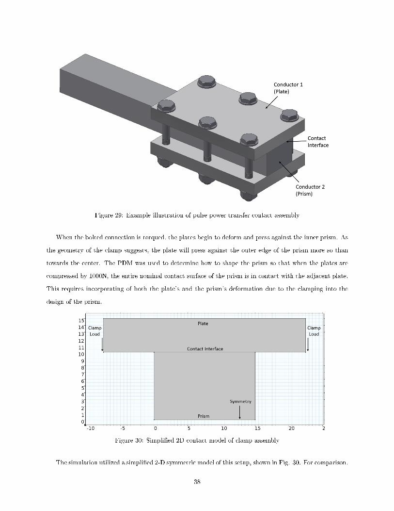
Figure 29: Example illustration of pulse power transfer contact assembly

When the bolted connection is torqued, the plates begin to deform and press against the inner prism. As

the geometry of the clamp suggests, the plate will press against the outer edge of the prism more so than

towards the center. The PDM was used to determine how to shape the prism so that when the plates are

compressed by 1000N, the entire nominal contact surface of the prism is in contact with the adjacent plate.

This requires incorporating of both the plate's and the prism's deformation due to the clamping into the

design of the prism.

Figure 30: Simpli�ed 2D contact model of clamp assembly

The simulation utilized a simpli�ed 2-D symmetric model of this setup, shown in Fig. 30. For comparison,

38

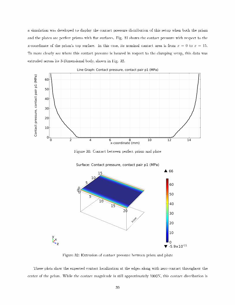
a simulation was developed to display the contact pressure distribution of this setup when both the prism

and the plates are perfect prisms with �at surfaces. Fig. 31 shows the contact pressure with respect to the

x-coordinate of the prism's top surface. In this case, its nominal contact area is from x = 0 to x = 15.

To more clearly see where this contact pressure is located in respect to the clamping setup, this data was

extruded across its 3-Dimensional body, shown in Fig. 32.

Figure 31: Contact between perfect prism and plate

Figure 32: Extrusion of contact pressure between prism and plate

These plots show the expected contact localization at the edges along with zero contact throughout the

center of the prism. While the contact magnitude is still approximately 1000N, this contact distribution is

39

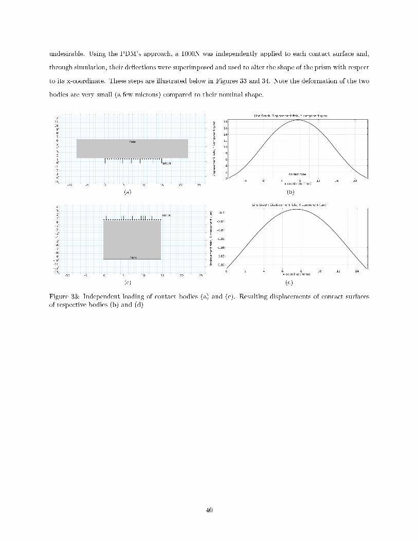
undesirable. Using the PDM's approach, a 1000N was independently applied to each contact surface and,

through simulation, their de�ections were superimposed and used to alter the shape of the prism with respect

to its x-coordinate. These steps are illustrated below in Figures 33 and 34. Note the deformation of the two

bodies are very small (a few microns) compared to their nominal shape.

(a) (b)

(c) (d)

Figure 33: Independent loading of contact bodies (a) and (c). Resulting displacements of contact surfacesof respective bodies (b) and (d)

40

Figure 34: Illustration of superimposing both de�ection responses to nominal prism shape to create PDMshape

This new prism shape allows for the continued use of the perfectly �at plates due to the alteration in the

prism shape accounting for both contacting body's deformation. Importing this new prism geometry into

COMSOL, the resulting contact plot from a 1000N load is shown below in Fig. 35. Comparing this result to

the same-scale plot in Fig. 31, one can see the drastic change in contact pressure distribution, noting that

both distributions have approximately a 1000N total magnitude.

Figure 35: Contact pressure between PDM shaped prism and plate at 1000N clamping force

41

6 Conclusions

Simulation results of the thin cylinders clamped together by a concentric nut and bolt supported the Predicted

Displacement Method's ability to improve contact pressure distribution. The series of simulations conducted

showed the expected behavior of the perfect cylinders in their localized contact around the bolt and the

induced gap between the cylinders along their outer areas. Those plots, Fig. 22 and 23, more clearly depict

how di�erent electrical contact resistance can be across the nominal contact surface. It was also shown how

improving this poor contact distribution was not a simple matter of further tightening of the nut and bolt,

shown in Fig. 24.

The PDM not only was able to make the contact pressure nearly uniform across the cylinder's entire

nominal contact area, it was also able to control and predict the resulting magnitude of this uniform contact.

The 200 Newtons of contact between the cylinders was chosen based on the geometry and size of this

example system. This contact magnitude can be chosen by design engineers in accordance to their design

requirements. The PDM can be used on any desired contact force assuming system components remain in

their linear-elastic behavior range.

Over-tightening was also investigated in the cylinder example because the Predicted Displacement Method

is dependent on a chosen contact design goal. Fig. 24 shows how the nearly perfect contact is only achieved

when loaded to the per-determined contact magnitude. This aspect was expected due to the procedures

included in the PDM. However, the results showed that even when over-tightened to twice the design value,

the contact pressure was still improved and more desirable than the non-PDM shape. Speci�cally, the PDM

disk made contact across its entire nominal contact surface even when over tightened. While the distribution

is not uniform when over-tightened, the lack of space or gap between the surfaces drastically decreases

contact resistance. These results show the PDM still aids in improving contact even when it is not perfectly

implemented, adding to its value as a design tool.

Comparing the results of the perfect disk contact and PDM disk contact highlights the reduced peak

stress seen by the contact body. By spreading out the contact pressure, the base material does not have

small areas of concentrated stress. This can expand the capability of a particular design or assembly by

mitigating areas of potential material yield or failure.

The following example investigated also demonstrated the PDM's success in controlling the contact

pressure and magnitude. The similar result of nearly uniform contact across this completely di�erent contact

interface promotes the PDM's value in its ability to be used on any assembly or contact interface. The steps

in the PDM do not change with geometry. Fundamentally, this method can be applied to any surface and the

plate-prism assembly supports this conclusion. More examples outside the scope of this work were analyzed

42

and the results were found to be consistent with the results presented here. Simulation results show that

the PDM can be used to produce uniform contact pressure across any contact surface.

The results in this work also identify some limitations of the Predicted Displacement Method. The

proof of concept compared the contact result of a PDM shaped beam with a beam shaped by a 4th order

approximation of the PDM shape. The di�erence between these two beam shapes are seen in a residual plot

found in Fig. 7. This residual plot shows how close the two curves are, only a few microns in di�erence.

However this subtle change in beam shape had a signi�cant e�ect on the resulting contact pressure. The

contact distribution shown in Fig. 19 is far from a controlled and desirable pressure distribution. These

results identify how sensitive the PDM is to accurate surface shape. However, this behavior is expected.

Contact mechanics is a phenomenon that is examined to the microscopic level. A di�erence in shape that is

beyond the magnitude of surface asperities is expected to overwhelm and control the contact behavior. It is

noted that the fourth order contact plot resembles the residual plot in the locations of high contact pressure

and positive residual material.

Another limitation of the PDM, as well as a limitation to the sensitivity observation previously noted, is

the accuracy of the numerical solvers used in simulation software. The di�erence between simulation results

and real-world actualities is inherently a complex thing to identify. Most all boundary conditions in FEA

are approximations to real world conditions, adding inherent di�erences. Additionally, numerical solvers

that solve non-linear simultaneous equations found in contact simulations are approximate solutions due

to no existing analytical solution. When properly used, Finite Element Analysis solution error is typically

insigni�cant. However, contact behavior is very sensitive to detail and small di�erences in models can cause

large changes in results.

Lastly, the PDM is limited to static analysis. The work done to analyze the feasibility of the PDM did

not include dynamic or time dependent situations. This concern, however, can be addressed in the design

phase, where the PDM is intended to be used. It is not uncommon for contact interfaces to have additional

life time maintenance requirements to ensure proper life time performance.

In conclusion, this work's contribution to science is a powerful methodology that gives engineers the

ability to speci�cally design contact interfaces for optimal contact, which an one day be implemented into

software programs. The results shown in this work suggest the PDM can provide more desirable contact

interfaces while maintaining desired contact magnitude. With this tool, contact interfaces can be designed to

support speci�c applications of unique contact assemblies. Future work of this idea includes 3-Dimensional

simulations and physical experimentation.

43

References

[1] R. S. Timsit, �Electrical contact resistance: Properties of stationary interfaces,� IEEE Components,

Packaging, and Manufacturing Technology Society, vol. 22, no. 1, pp. 85�98, 1999.

[2] P. G. Slade, Concequences of Arcing, 1999.

[3] D. Feng, J. He, L. Chen, S. Xia, Z. Xiao, J. Li, , and P. Yan, �Study on the curve shape of c-shaped

armatures trailing arms in rectangular bore railgun,� IEEE TRANSACTIONS ON PLASMA SCIENCE,

vol. 41, no. 5, pp. 1460�1466, 2013.

[4] D. Feng, J. He, L. Chen, S. Xia, L. Tang, J. Li, , and P. Yan, �Investigations of the armature-rail contact

pressure distribution in a railgun,� IEEE TRANSACTIONS ON PLASMA SCIENCE, vol. 43, no. 5,

pp. 1657�1662, 2015.

[5] D. Feng, J. He, L. Chen, S. Xia, Z. Xiao, L. Tang, J. Li, and P. Yan, �Simulations on arc surfaced

c-shaped armatures for round-like bore railguns,� IEEE TRANSACTIONS ON PLASMA SCIENCE,

vol. 41, no. 5, pp. 1467�1474, 2013.

[6] J. Barber, Elasticity, 2001.

[7] X. Zhu, �Tutorial on hertz contact stress,� pp. 1�8, 2012.

[8] P. Wriggers, Computational Contact Mechanics, 2002.

[9] G.R.Cowper, �The shear coe�cient in timoshenkos beam theory,� ASME Journal of Applied Mechanics,

vol. 43, no. 2, pp. 335�340, 1966.

[10] U. Goerguelue, �Beam theories: The di�erence between euler-bernoulli and timoschenko,� Researchgate.

[11] S. Timoshenko and J. Goodier, Theory of Elasticity, 1970.

[12] K.-T. Hsieh, S. Satapathy, and M.-T. Hsieh, �E�ects of pressure-dependent contact resistivity on contact

interfacial conditions,� IEEE, 2008.

[13] R. Holm, Electric contacts: theory and application, 1967.

[14] R. G. Budynas and J. K. Nisbett, Shigley's Mechanical Engineering Design 9th Ed., 2011.

[15] K. Johnson, Contact Mechanics, 1985.

[16] C. E. Augarde and A. J. Deeks, �The use of timoshenkos exact solution for a cantilever beam in adaptive

analysis,� SCIENCEDirect, pp. 1�7, 2008.

44