Consumer Behavior

Overview

I. Consumer BehaviorIndifference Curve AnalysisConsumer Preference Ordering

II. ConstraintsThe Budget ConstraintChanges in IncomeChanges in Prices

III. Consumer EquilibriumIV. Indifference Curve Analysis & Demand

CurvesIndividual DemandMarket Demand

4-2

Consumer BehaviorConsumer Opportunities

The possible goods and services consumer can afford to consume.

Consumer PreferencesThe goods and services consumers actually

consume.Given the choice between 2 bundles of

goods a consumer either Prefers bundle A to bundle B: A B.Prefers bundle B to bundle A: A B.Is indifferent between the two: A B.

4-3

Indifference Curve Analysis

Indifference CurveA curve that defines the combinations of

2 or more goods that give a consumer the same level of satisfaction.

Assumptions:1.Resources are limited2.Resources are fully utilized3. Only 2 products can be produced at

a time4.Technology remains the same5.Satisfaction level remains same on the

same indifference curve

Marginal Rate of SubstitutionThe rate at which a consumer is willing

to substitute one good for another and maintain the same satisfaction level.

I.

II.

III.

Good Y

Good X

4-4

Consumer Preference Ordering Properties

CompletenessMore is BetterDiminishing Marginal Rate of SubstitutionTransitivity

4-5

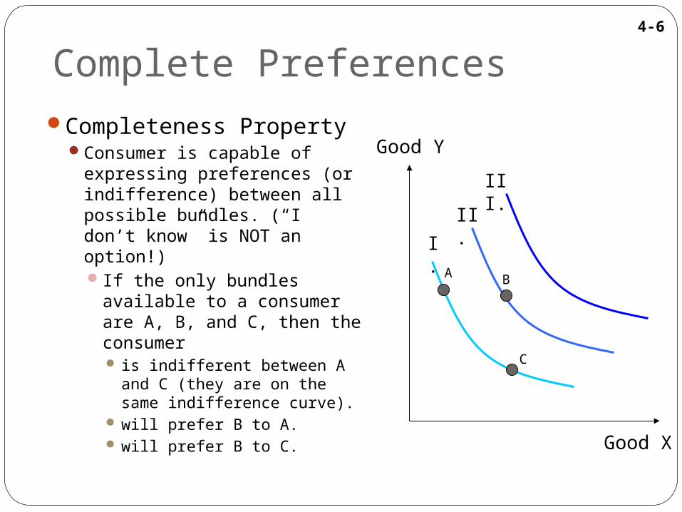
Complete PreferencesCompleteness Property

Consumer is capable of expressing preferences (or indifference) between all possible bundles. (“I don’t know” is NOT an option!)If the only bundles

available to a consumer are A, B, and C, then the consumer is indifferent between A

and C (they are on the same indifference curve).

will prefer B to A. will prefer B to C.

I.

II.

III.

Good Y

Good X

A

C

B

4-6

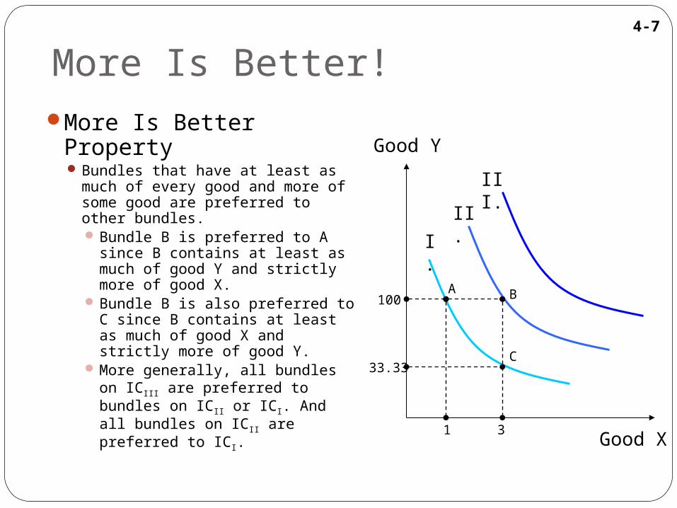
More Is Better!More Is Better Property

Bundles that have at least as much of every good and more of some good are preferred to other bundles. Bundle B is preferred to A since

B contains at least as much of good Y and strictly more of good X.

Bundle B is also preferred to C since B contains at least as much of good X and strictly more of good Y.

More generally, all bundles on ICIII are preferred to bundles on ICII or ICI. And all bundles on ICII are preferred to ICI.

I.

II.

III.

Good Y

Good X

A

C

B

1

33.33

100

3

4-7

Diminishing Marginal Rate of SubstitutionMarginal Rate of

Substitution The amount of good Y the consumer is

willing to give up to maintain the same satisfaction level decreases as more of good X is acquired.

The rate at which a consumer is willing to substitute one good for another and maintain the same satisfaction level.

To go from consumption bundle A to B the consumer must give up 50 units of Y to get one additional unit of X.

To go from consumption bundle B to C the consumer must give up 16.67 units of Y to get one additional unit of X.

To go from consumption bundle C to D the consumer must give up only 8.33 units of Y to get one additional unit of X.

I.

II.

III.

Good Y

Good X1 3 42

100

50

33.33 25

A

B

CD

4-8

Consistent Bundle OrderingsTransitivity Property

For the three bundles A, B, and C, the transitivity property implies that if C B and B A, then C A.

Transitive preferences along with the more-is-better property imply thatindifference curves will

not intersect.the consumer will not get

caught in a perpetual cycle of indecision.

I.

II.

III.

Good Y

Good X21

100

5

50

7

75

A

B

C

4-9

The Budget ConstraintOpportunity Set

The set of consumption bundles that are affordable.PxX + PyY M.

Budget LineThe bundles of goods that

exhaust a consumers income.PxX + PyY = M.

Market Rate of SubstitutionThe slope of the budget line

-Px / Py

Y

X

The Opportunity Set

Budget Line

Y = M/PY – (PX/PY)XM/PY

M/PX

4-10

Changes in the Budget Line

Changes in IncomeIncreases lead to a parallel,

outward shift in the budget line (M1 > M0).

Decreases lead to a parallel, downward shift (M2 < M0).

Changes in PriceA decreases in the price of

good X rotates the budget line counter-clockwise (PX0

>

PX1).

An increases rotates the budget line clockwise (not shown).

X

Y

X

YNew Budget Line for a price decrease.

M0/PY

M0/PX

M2/PY

M2/PX

M1/PY

M1/PX

M0/PY

M0/PX0M0/PX1

4-11

Consumer Equilibrium

The equilibrium consumption bundle is the affordable bundle that yields the highest level of satisfaction.Consumer equilibrium

occurs at a point whereMRS = PX / PY.

Equivalently, the slope of the indifference curve equals the budget line. I.

II.

III.

X

Y

Consumer Equilibrium

M/PY

M/PX

4-12

Price Changes and Consumer Equilibrium

Substitute GoodsAn increase (decrease) in the price of good X

leads to an increase (decrease) in the consumption of good Y.Examples:

Coke and Pepsi.Complementary Goods

An increase (decrease) in the price of good X leads to a decrease (increase) in the consumption of good Y.Examples:

Computer CPUs and monitors.

4-13

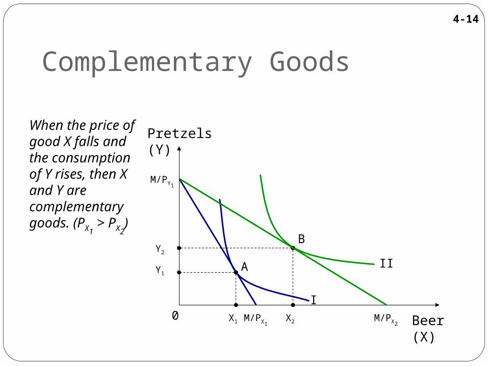
Complementary Goods

When the price of good X falls and the consumption of Y rises, then X and Y are complementary goods. (PX1

> PX2)

Pretzels (Y)

Beer (X)

II

I0

Y2

Y1

X1 X2

A

B

M/PX1M/PX2

M/PY1

4-14

Income Changes and Consumer Equilibrium

Normal GoodsGood X is a normal good if an increase

(decrease) in income leads to an increase (decrease) in its consumption.

Inferior GoodsGood X is an inferior good if an increase

(decrease) in income leads to a decrease (increase) in its consumption.

4-15

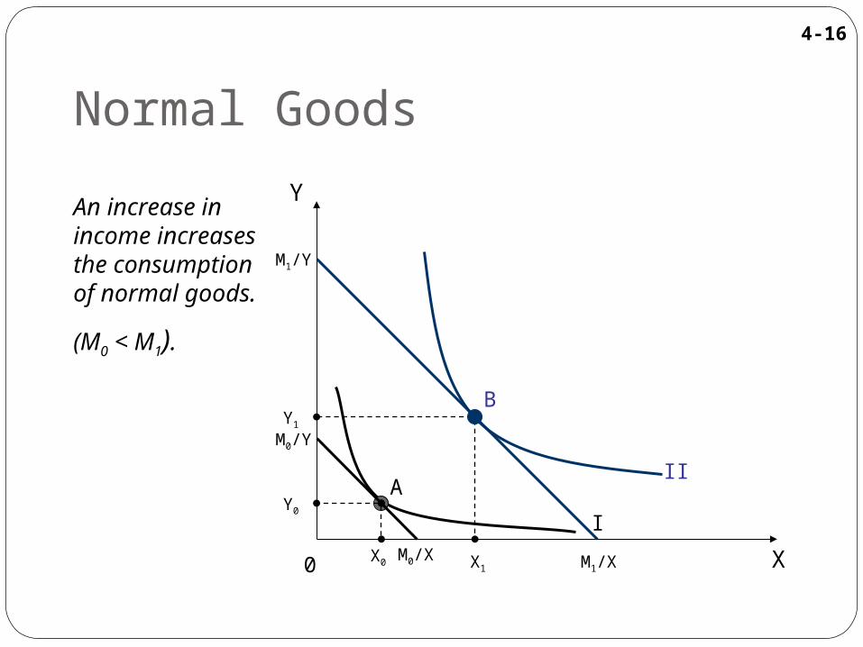
Normal Goods

An increase in income increases the consumption of normal goods.

(M0 < M1).

Y

II

I

0

A

B

X

M0/Y

M0/X

M1/Y

M1/XX0

Y0

X1

Y1

4-16

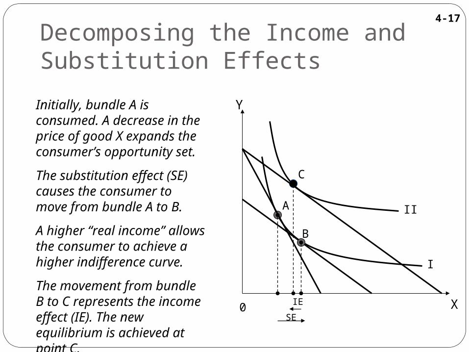
Decomposing the Income and Substitution Effects

Initially, bundle A is consumed. A decrease in the price of good X expands the consumer’s opportunity set.

The substitution effect (SE) causes the consumer to move from bundle A to B.

A higher “real income” allows the consumer to achieve a higher indifference curve.

The movement from bundle B to C represents the income effect (IE). The new equilibrium is achieved at point C.

Y

II

I

0

A

X

C

B

SE

IE

4-17

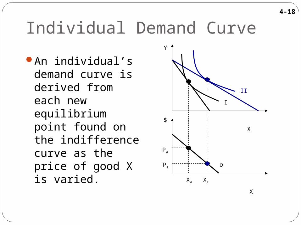
Individual Demand Curve

An individual’s demand curve is derived from each new equilibrium point found on the indifference curve as the price of good X is varied.

X

Y

$

X

D

II

I

P0

P1

X0 X1

4-18

Market DemandThe market demand curve is the horizontal

summation of individual demand curves.It indicates the total quantity all consumers

would purchase at each price point.

Q

$ $

Q

50

40

D2D1

Individual Demand Curves

Market Demand Curve

1 2 1 2 3

DM

4-19

ConclusionIndifference curve properties reveal

information about consumers’ preferences between bundles of goods.Completeness.More is better.Diminishing marginal rate of substitution.Transitivity.

Indifference curves along with price changes determine individuals’ demand curves.

Market demand is the horizontal summation of individuals’ demands.

4-20