
Construction Heuristics for the Airline Taxi Problem
211
Construction Heuristics for the Airline Taxi Problem Ian Michael Dougal Campbell A thesis submitted to the Faculty of Engineering and the Built Environment, Uni- versity of the Witwatersrand, Johannesburg, in fulfilment of the requirements for the degree of Doctor of Philosophy. Johannesburg, October 2013
Transcript of Construction Heuristics for the Airline Taxi Problem

Construction Heuristics for the
Airline Taxi Problem
Ian Michael Dougal Campbell
A thesis submitted to the Faculty of Engineering and the Built Environment, Uni-
versity of the Witwatersrand, Johannesburg, in fulfilment of the requirements for
the degree of Doctor of Philosophy.
Johannesburg, October 2013
Declaration
I declare that this thesis is my own, unaided work, except where otherwise acknowl-
edged. It is being submitted for the degree of Doctor of Philosophy in the University
of the Witwatersrand, Johannesburg. It has not been submitted before for any de-
gree or examination at any other university.
Signed this day of 20
Ian Michael Dougal Campbell.
i

Acknowledgements
Firstly, I would like to thank my parents, my sister and my brothers for many years
of love and support.
Secondly, special thanks to my supervisor, Prof. M.M. Ali, for his unwavering and
motivational guidance and support, as well as his patience in wading repeatedly
through this tome and his resulting comments and corrections.
Thirdly, many thanks to Margaret Campbell and Prof. Robert Reid for their com-
prehensive proof reading and valuable corrections.
ii
Abstract
A literature review of vehicle routing problems (VRPs) in general, and specifically
airline scheduling problems and the airline taxi problem, is provided. A real-world
airline taxi scheduling problem is described as experienced by a tourist airline oper-
ating in the Okavango Delta, Botswana. In this problem, a daily schedule is drawn
up manually by a team of experienced schedulers a few days before the day in ques-
tion. In this research, a slightly relaxed version of the problem is considered in order
to develop heuristics and modelling methods which will be useful for general cases.
Various methods and heuristics are proposed for the problem and tested on a small
version of the problem as well as the full-sized version. The most promising methods
are demonstrated and solutions provided. One of the methods was applied to the
actual problem to demonstrate the practical usefulness. In this case a schedule with
a cost 12% lower than the manual schedule cost was achieved. All the heuristics and
methods are applicable to certain other VRPs, particularly real-world or highly-
constrained VRPs. An example is provided of a solution method for a real-world
instance of the multi-vehicle capacitated vehicle routing problem (MVCVRP). An-
other example is provided of a standard, benchmark instance from the internet of a
capacitated vehicle routing problem with time windows (CVRPTW).
iii
Contents
Declaration i
Acknowledgements ii
Abstract iii
Contents iv
List of Figures ix
List of Tables x
1 Introduction 1
1.1 Scheduling in Commercial Scheduled Airlines . . . . . . . . . . . . . 1
1.2 On-Demand Airline Scheduling . . . . . . . . . . . . . . . . . . . . . 2
1.3 Research Motivation . . . . . . . . . . . . . . . . . . . . . . . . . . . 3
2 Objectives 5
3 Literature Review 6
3.1 Vehicle Routing . . . . . . . . . . . . . . . . . . . . . . . . . . . . . . 6
3.1.1 Types of Vehicle Routing Problems . . . . . . . . . . . . . . . 6
iv

3.1.2 Solving VRPs . . . . . . . . . . . . . . . . . . . . . . . . . . . 11
3.2 Airline Scheduling . . . . . . . . . . . . . . . . . . . . . . . . . . . . 35
3.2.1 Scheduled Airlines . . . . . . . . . . . . . . . . . . . . . . . . 35
3.2.2 Charter Airlines . . . . . . . . . . . . . . . . . . . . . . . . . 41
3.2.3 On-Demand Air Transportation . . . . . . . . . . . . . . . . . 41
3.3 Solving large MIP problems . . . . . . . . . . . . . . . . . . . . . . . 44
3.4 Conclusions from Literature Review . . . . . . . . . . . . . . . . . . 46
4 Methodology 47
4.1 Overview . . . . . . . . . . . . . . . . . . . . . . . . . . . . . . . . . 47
4.2 Small-Scale Benchmark Airline Taxi Problem . . . . . . . . . . . . . 49
4.3 Sefofane Air Solution . . . . . . . . . . . . . . . . . . . . . . . . . . . 50
4.4 Application to Other VRPs . . . . . . . . . . . . . . . . . . . . . . . 50
5 The Sefofane Air Scheduling Problem Description 52
5.1 Sefofane Air Operations . . . . . . . . . . . . . . . . . . . . . . . . . 52
5.2 Problem Specifications . . . . . . . . . . . . . . . . . . . . . . . . . . 53
6 Multi-Commodity Network Flow ILP with Time Discretisations 59
6.1 Description . . . . . . . . . . . . . . . . . . . . . . . . . . . . . . . . 59
7 Heuristics for Problem Size Reduction 64
7.1 Motivation . . . . . . . . . . . . . . . . . . . . . . . . . . . . . . . . 64
7.2 Group Aggregation Heuristic . . . . . . . . . . . . . . . . . . . . . . 65
7.2.1 Description . . . . . . . . . . . . . . . . . . . . . . . . . . . . 65
v

7.2.2 Aggregation Validation . . . . . . . . . . . . . . . . . . . . . 66
7.3 Geographic Heuristic . . . . . . . . . . . . . . . . . . . . . . . . . . . 66
7.3.1 Description . . . . . . . . . . . . . . . . . . . . . . . . . . . . 66
7.3.2 Evaluation of Geographic Heuristic Effect . . . . . . . . . . . 68
7.4 MCNFP Solutions . . . . . . . . . . . . . . . . . . . . . . . . . . . . 69
7.4.1 Small Schedule . . . . . . . . . . . . . . . . . . . . . . . . . . 69
7.4.2 Full Schedule . . . . . . . . . . . . . . . . . . . . . . . . . . . 72
7.5 Discussion . . . . . . . . . . . . . . . . . . . . . . . . . . . . . . . . . 73
8 Agent Routing Variable Generation 76
8.1 Description . . . . . . . . . . . . . . . . . . . . . . . . . . . . . . . . 76
8.2 Observations and Results . . . . . . . . . . . . . . . . . . . . . . . . 83
8.3 Discussion . . . . . . . . . . . . . . . . . . . . . . . . . . . . . . . . . 87
9 Composite Variable Formulation 88
9.1 Description . . . . . . . . . . . . . . . . . . . . . . . . . . . . . . . . 88
9.2 Observations and Results . . . . . . . . . . . . . . . . . . . . . . . . 93
9.2.1 Small Schedule . . . . . . . . . . . . . . . . . . . . . . . . . . 93
9.2.2 Full Schedule . . . . . . . . . . . . . . . . . . . . . . . . . . . 95
9.3 Discussion . . . . . . . . . . . . . . . . . . . . . . . . . . . . . . . . . 95
10 The Sefofane Air Scheduling Problem 97
10.1 Constrained Problem . . . . . . . . . . . . . . . . . . . . . . . . . . . 97
10.2 Results and Discussion . . . . . . . . . . . . . . . . . . . . . . . . . . 100
vi
11 Other VRPs 102
11.1 Introduction . . . . . . . . . . . . . . . . . . . . . . . . . . . . . . . . 102
11.2 Multi Vehicle CVRP (MVCVRP) . . . . . . . . . . . . . . . . . . . . 102
11.2.1 Problem Description . . . . . . . . . . . . . . . . . . . . . . . 102
11.2.2 Exact ILP Formulation . . . . . . . . . . . . . . . . . . . . . 103
11.2.3 Composite Variable Formulation . . . . . . . . . . . . . . . . 106
11.2.4 Methodology . . . . . . . . . . . . . . . . . . . . . . . . . . . 108
11.2.5 Observations and Results . . . . . . . . . . . . . . . . . . . . 109
11.2.6 Discussion . . . . . . . . . . . . . . . . . . . . . . . . . . . . . 110
11.3 Capacitated Vehicle Routing Problem with Time Windows (CVRPTW)110
11.3.1 Problem Description . . . . . . . . . . . . . . . . . . . . . . . 110
11.3.2 Variable Generation . . . . . . . . . . . . . . . . . . . . . . . 111
11.3.3 Observations, Results and Discussion . . . . . . . . . . . . . . 116
12 Conclusions 117
13 Recommendations 120
REFERENCES 121
APPENDIX A Sefofane Air Problem Data 134
APPENDIX B Manual Schedule 140
APPENDIX C Aggregation Heuristic Result 145
vii

APPENDIX D Agent Routing MATLAB Code - Airline Taxi Prob-
lem 148
D.1 Attractiveness Parameters . . . . . . . . . . . . . . . . . . . . . . . . 148
D.2 Agent Routing Function . . . . . . . . . . . . . . . . . . . . . . . . . 148
APPENDIX E Agent-Generated Variable Schedule 169
APPENDIX F Automated Composite Schedule 172
APPENDIX G MVCVRP Data 175
G.1 Problem Data . . . . . . . . . . . . . . . . . . . . . . . . . . . . . . . 175
G.2 Supplied Delivery Lists . . . . . . . . . . . . . . . . . . . . . . . . . . 180
G.2.1 List for Day 1 . . . . . . . . . . . . . . . . . . . . . . . . . . . 180
G.2.2 List for Day 2 . . . . . . . . . . . . . . . . . . . . . . . . . . . 182
G.2.3 List for Day 3 . . . . . . . . . . . . . . . . . . . . . . . . . . . 186
APPENDIX H Agent Routing MATLAB Code - CVRPTW 190
APPENDIX I CVRPTW Data 196
viii
List of Figures
3.1 An Insertion Heuristic . . . . . . . . . . . . . . . . . . . . . . . . . . 13
3.2 A Savings Heuristic . . . . . . . . . . . . . . . . . . . . . . . . . . . . 13
3.3 2-Opt Exchange Move . . . . . . . . . . . . . . . . . . . . . . . . . . 16
3.4 Multi Agent Cooperative Search . . . . . . . . . . . . . . . . . . . . 23
3.5 GPDP Classification . . . . . . . . . . . . . . . . . . . . . . . . . . . 25
3.6 Time-Space Network . . . . . . . . . . . . . . . . . . . . . . . . . . . 36
3.7 Time-Space Network with Time Discretisations . . . . . . . . . . . . 38
5.1 Cessna C206 . . . . . . . . . . . . . . . . . . . . . . . . . . . . . . . 53
5.2 Cessna C208 Grand Caravan . . . . . . . . . . . . . . . . . . . . . . 54
5.3 Map of the Okavango Delta Area . . . . . . . . . . . . . . . . . . . . 56
7.1 Geographic Heuristic . . . . . . . . . . . . . . . . . . . . . . . . . . . 67
8.1 Agent Routing Method Modelling Process . . . . . . . . . . . . . . . 84
9.1 Linking of Two Flight Variables (Dual Linking) . . . . . . . . . . . . 89
9.2 Composite Variable Modelling Method . . . . . . . . . . . . . . . . . 91
ix

List of Tables
3.1 VRP Taxonomic Review . . . . . . . . . . . . . . . . . . . . . . . . 9
3.2 Metaheurstics . . . . . . . . . . . . . . . . . . . . . . . . . . . . . . . 19
3.3 Genetic Algorithm Approaches to the VRPTW . . . . . . . . . . . . 22
3.4 DARP Heuristics . . . . . . . . . . . . . . . . . . . . . . . . . . . . . 27
3.5 DARP Metaheuristics . . . . . . . . . . . . . . . . . . . . . . . . . . 32
5.1 Fleet Characteristics . . . . . . . . . . . . . . . . . . . . . . . . . . . 54
7.1 Cost and Computation Times for Different Geographic Heuristic Pa-
rameters, Small Schedule . . . . . . . . . . . . . . . . . . . . . . . . 68
7.2 Effect of Geographic Heuristic on Number of Variables for Large
Schedule . . . . . . . . . . . . . . . . . . . . . . . . . . . . . . . . . . 69
7.3 Small Schedule Solution . . . . . . . . . . . . . . . . . . . . . . . . . 71
7.4 Multi-Leg Trips - Unlimited Ground Waiting Time, Small Schedule 71
7.5 Multi-Leg Trips - Minimum Ground Waiting Time, Small Schedule 72
7.6 Schedule Cost Results Summary for Small Schedule . . . . . . . . . 72
7.7 Multi-Legs Trips for Large Schedule . . . . . . . . . . . . . . . . . . 73
7.8 Schedule Cost Results Summary for Large Schedule . . . . . . . . . 73
8.1 Full Schedule Solutions . . . . . . . . . . . . . . . . . . . . . . . . . . 85
x
8.2 Aircraft Changes and Ground Waiting Times . . . . . . . . . . . . . 86
8.3 Aircraft Changes and Ground Waiting Times with Passenger Group
Time Cost Modified Objective Function . . . . . . . . . . . . . . . . 86
8.4 Aircraft Changes and Ground Waiting Times with Individual Passen-
ger Time Cost Modified Objective Function . . . . . . . . . . . . . . 86
9.1 Small Schedule Costs Using Composite Variables . . . . . . . . . . . 94
9.2 Small Schedule Using Composite Variables . . . . . . . . . . . . . . . 94
9.3 Full Schedule Costs Using Composite Variables with Constrained
End-Of-Day Aircraft Locations . . . . . . . . . . . . . . . . . . . . . 95
9.4 Comparison Solutions - Unconstrained End-of-Day Aircraft Positions 96
11.1 Customers for Small Version . . . . . . . . . . . . . . . . . . . . . . . 108
11.2 Fleet Description . . . . . . . . . . . . . . . . . . . . . . . . . . . . . 108
11.3 MVCVRP Solutions . . . . . . . . . . . . . . . . . . . . . . . . . . . 110
A.1 Full Schedule . . . . . . . . . . . . . . . . . . . . . . . . . . . . . . . 135
A.2 Distance matrix . . . . . . . . . . . . . . . . . . . . . . . . . . . . . 138
A.3 Aircraft and Loadmaster Day Start and End Positions . . . . . . . . 139
A.4 Airport Codes and Assigned Numbers . . . . . . . . . . . . . . . . . 139
B.1 Manual Schedule . . . . . . . . . . . . . . . . . . . . . . . . . . . . . 141
C.1 Aggregated Groups for Full Schedule . . . . . . . . . . . . . . . . . . 146
E.1 Agent Routing Method Automated Full Schedule . . . . . . . . . . . 170
F.1 Composite Variable Method Automated Full Schedule . . . . . . . . 173
xi

G.1 Large MVCVRP Instance . . . . . . . . . . . . . . . . . . . . . . . . 176
G.2 Large MVCVRP Instance - Vehicles . . . . . . . . . . . . . . . . . . 178
G.3 Medium MVCVRP Instance - Customers . . . . . . . . . . . . . . . 179
G.4 Medium MVCVRP Instance - Vehicles . . . . . . . . . . . . . . . . . 179
I.1 Solomon Data RC101 . . . . . . . . . . . . . . . . . . . . . . . . . . 197
xii
1 Introduction
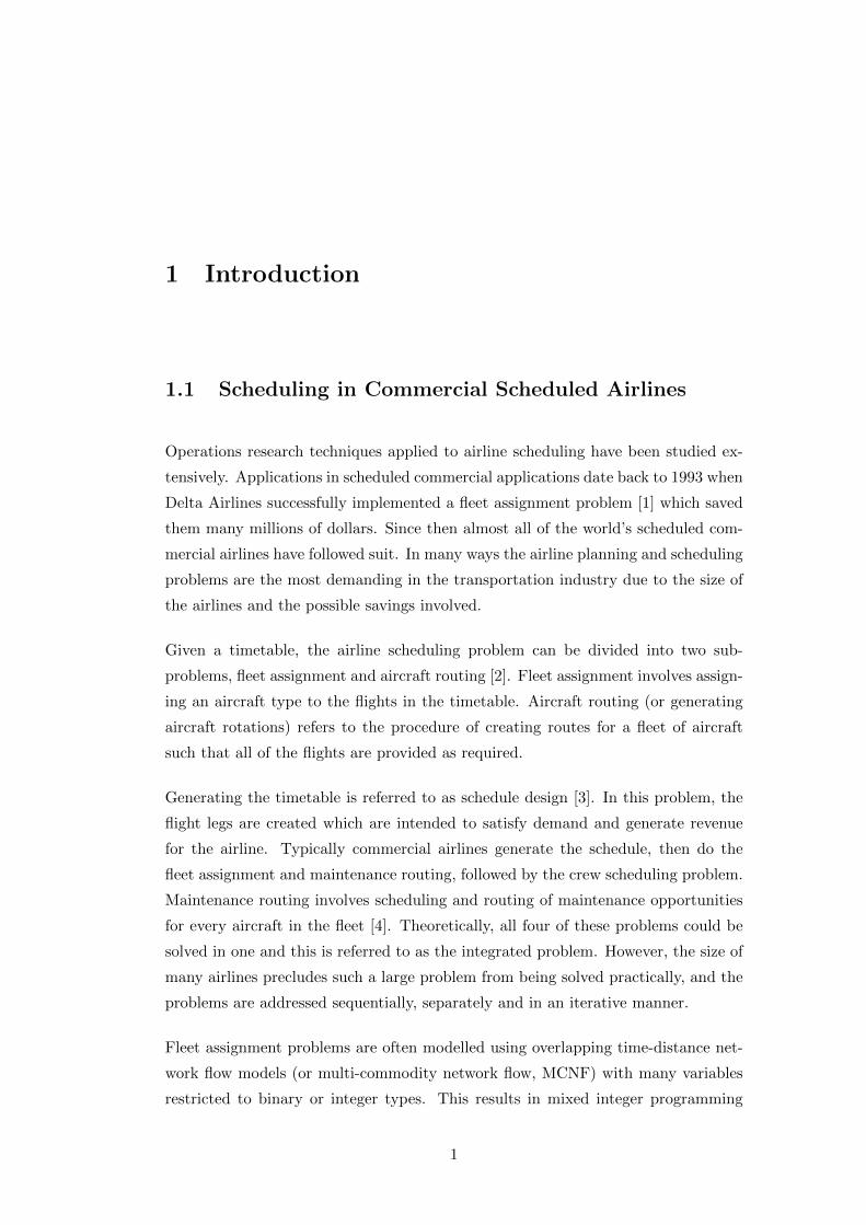
1.1 Scheduling in Commercial Scheduled Airlines
Operations research techniques applied to airline scheduling have been studied ex-
tensively. Applications in scheduled commercial applications date back to 1993 when
Delta Airlines successfully implemented a fleet assignment problem [1] which saved
them many millions of dollars. Since then almost all of the world’s scheduled com-
mercial airlines have followed suit. In many ways the airline planning and scheduling
problems are the most demanding in the transportation industry due to the size of
the airlines and the possible savings involved.
Given a timetable, the airline scheduling problem can be divided into two sub-
problems, fleet assignment and aircraft routing [2]. Fleet assignment involves assign-
ing an aircraft type to the flights in the timetable. Aircraft routing (or generating
aircraft rotations) refers to the procedure of creating routes for a fleet of aircraft
such that all of the flights are provided as required.
Generating the timetable is referred to as schedule design [3]. In this problem, the
flight legs are created which are intended to satisfy demand and generate revenue
for the airline. Typically commercial airlines generate the schedule, then do the
fleet assignment and maintenance routing, followed by the crew scheduling problem.
Maintenance routing involves scheduling and routing of maintenance opportunities
for every aircraft in the fleet [4]. Theoretically, all four of these problems could be
solved in one and this is referred to as the integrated problem. However, the size of
many airlines precludes such a large problem from being solved practically, and the
problems are addressed sequentially, separately and in an iterative manner.
Fleet assignment problems are often modelled using overlapping time-distance net-
work flow models (or multi-commodity network flow, MCNF) with many variables
restricted to binary or integer types. This results in mixed integer programming
1

(MIP) models with large numbers of variables and constraints. Because of the com-
putational effort involved, solutions can take impractically long times to achieve.
Much effort has been spent on techniques to solve these problems within reasonable
time limits.
Passenger airlines might only design and optimize their schedule once from scratch.
This is called ‘cold start’ [1]. Such models can be huge and take hours if not days
to run. In most cases, a previously designed feasible schedule is optimized (‘warm
start’) which results in much faster solution times. A schedule sometimes repeats
itself daily and/or weekly and does not change for months. Changes that are imple-
mented are normally small.
1.2 On-Demand Airline Scheduling
Certain charter airlines schedule their aircraft to satisfy some demand such as that
generated by a once off event, e.g. a sporting event. In this case, the objective is to
maximize profit and the demand does not necessarily have to be completely satisfied.
Either the group requiring the transport will hire the plane to accommodate all group
members, or the charter company will schedule a special trip to meet the demand,
for example, from multiple groups.
The airline taxi scheduling problem is different in that demand must be met com-
pletely at the lowest cost possible. An airline taxi service is operated by a charter
airline company called Sefofane Air in the Okavango Delta region in Botswana. The
extensive waterways that make up this geographical feature make land transport
difficult and often impossible. In addition the authorities have legislated that pas-
sengers must be ferried between the various tourist camps by aircraft to minimize
environmental effects. Therefore small groups of tourists must be ferried by air-
craft between places of interest or accommodation according to a schedule that has
previously been designed by a tour operator and paid for by the client (passengers).
The schedule for such an airline changes completely every day. Often the next
day’s schedule needs to be designed from scratch. Currently, these schedules are
generated manually by a team of experienced people. Growth of airline traffic and
risks with regard to the possibility of losing scheduling staff has created the need to
automatically create good schedules and to reduce aircraft operation and scheduling
costs. Sefofane Air must satisfy 158 bookings on a busy day, using 14 aircraft of two
different types and serving 21 destinations.
2
There are some other similar or closely-related problems in the literature, namely
the static dial-a-flight problem (SDAFP) [5], air taxi [6] or per-seat, on-demand
(PSOD) air transportation problem [7]. The problems described appear to be largely
similar, therefore the Sefofane Air scheduling problem can be classed in vehicle
routing literature accordingly.
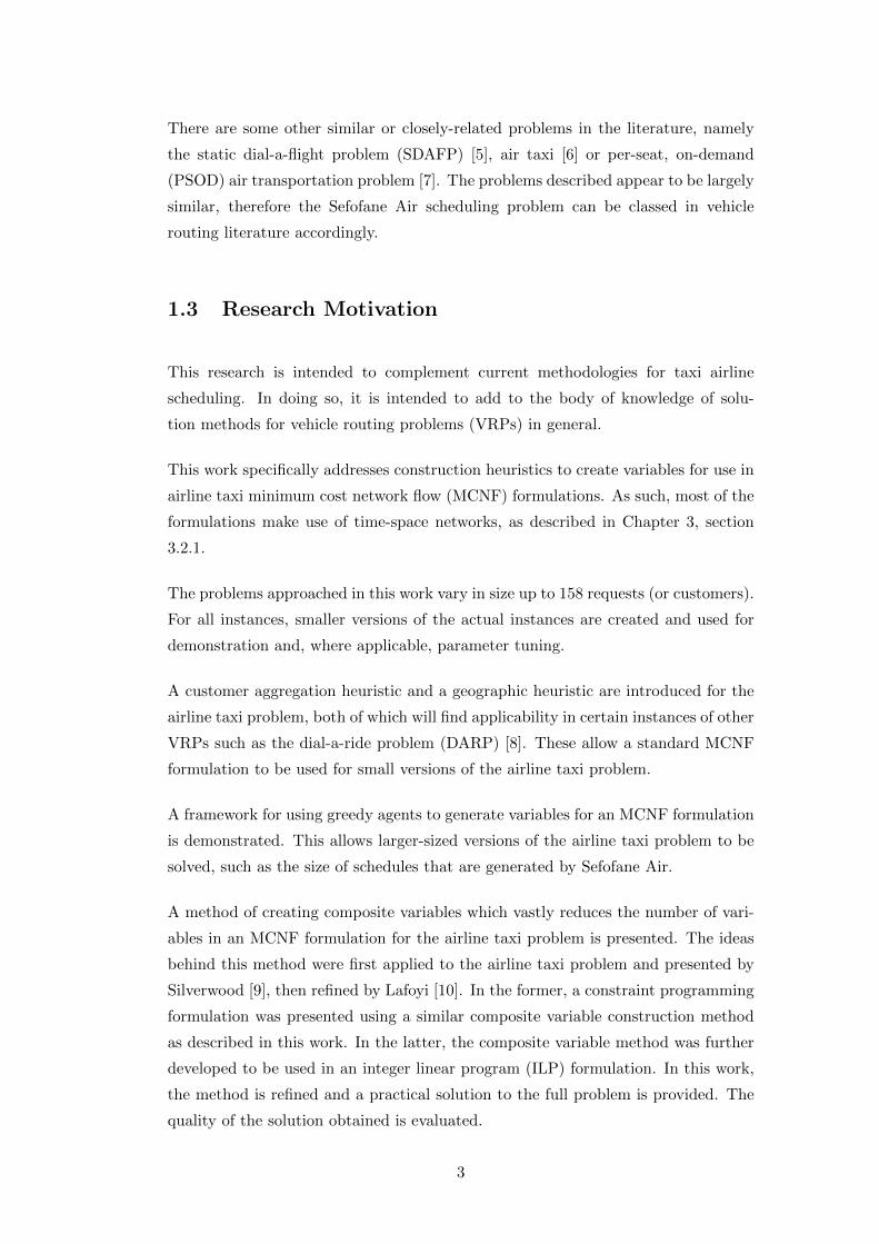
1.3 Research Motivation
This research is intended to complement current methodologies for taxi airline
scheduling. In doing so, it is intended to add to the body of knowledge of solu-
tion methods for vehicle routing problems (VRPs) in general.
This work specifically addresses construction heuristics to create variables for use in
airline taxi minimum cost network flow (MCNF) formulations. As such, most of the
formulations make use of time-space networks, as described in Chapter 3, section
3.2.1.
The problems approached in this work vary in size up to 158 requests (or customers).
For all instances, smaller versions of the actual instances are created and used for
demonstration and, where applicable, parameter tuning.
A customer aggregation heuristic and a geographic heuristic are introduced for the
airline taxi problem, both of which will find applicability in certain instances of other
VRPs such as the dial-a-ride problem (DARP) [8]. These allow a standard MCNF
formulation to be used for small versions of the airline taxi problem.
A framework for using greedy agents to generate variables for an MCNF formulation
is demonstrated. This allows larger-sized versions of the airline taxi problem to be
solved, such as the size of schedules that are generated by Sefofane Air.
A method of creating composite variables which vastly reduces the number of vari-
ables in an MCNF formulation for the airline taxi problem is presented. The ideas
behind this method were first applied to the airline taxi problem and presented by
Silverwood [9], then refined by Lafoyi [10]. In the former, a constraint programming
formulation was presented using a similar composite variable construction method
as described in this work. In the latter, the composite variable method was further
developed to be used in an integer linear program (ILP) formulation. In this work,
the method is refined and a practical solution to the full problem is provided. The
quality of the solution obtained is evaluated.
3
Finally, it is shown that these methods offer alternative approaches to other VRPs.
This is done by tackling a real-world multi-vehicle capacitated vehicle routing prob-
lem (MVCVRP) [11] and a standard, benchmark VRP with time windows obtained
from the Internet.
The airline taxi problem addressed is an actual, real-world problem, and as such is
highly constrained with operational requirements. Similarly, the MVCVRP in Chap-
ter 11 is a real-world problem described by the company concerned. The VRPTW
in Chapter 11 is a problem artificially created specifically to be a benchmark prob-
lem, and as such it does not have the typical operational constraints of a real-world
problem (i.e. it is less highly constrained).
Results are presented showing the usefulness of the various methods proposed.
4

2 Objectives
This work was inspired by the Sefofane Air scheduling problem, which will be de-
scribed in more detail in Chapter 5. One objective is to provide practical methods
to solve that problem and demonstrate these methods. In order to achieve this,
methods to solve the airline taxi problem will be developed. Heuristics offer the
most viable methods to achieve this. This work will only deal with construction of
solutions, as opposed to solution improvement techniques and heuristics.
Therefore, the objectives are stated as follows:
• To develop and evaluate construction heuristic methods to solve the airline
taxi problem in general and the specific problem under consideration.
• To suggest and consider the use of such methods in other vehicle routing
problems.
5

3 Literature Review
3.1 Vehicle Routing
3.1.1 Types of Vehicle Routing Problems
There are a number of standard vehicle routing problems (VRPs) defined in the
literature, all classified as NP -hard and therefore difficult to solve, even for small
instances. In practice, such problems become increasingly more difficult to solve as
they grow in size, so keeping the number of variables to a minimum is important.
The travelling salesperson problem (TSP) is a problem where the shortest path
through a number of locations must be obtained, and each location is only visited
once. It is important because, although NP -hard, a number of efficient algorithms
have been developed for it, notably the famous Lin-Kernighan (L-K) heuristic algo-
rithm [12]. VRP solution methods often involve solving some sub-problem/s which
are TSPs.
TSPs, like VRPs, can be formulated as integer linear programs (ILPs), and solved as
such. If no heuristics are used, the solution is termed exact, since, if well-formulated,
the solution obtained is optimal. However the methods for solving ILPs are generally
based on branch and bound, which is a form of enumeration and therefore varies
in solution time for different instances. Solving can be slow, especially if there are
many variables and constraints.
The term VRP often refers to a delivery problem with depot and customers. Be-
cause of the difficulties in application of exact methods to practically-sized problems,
heuristics and metaheuristics are frequently applied. Variations of the VRP include
the capacitated VRP (CVRP) and the multi-vehicle CVRP (MVCVRP).
The CVRP involves using vehicles of one type, but with limited capacity, to deliver
goods from a depot to a number of customers. The CVRP with time windows
6

(CVRPTW) is similar, but with the addition of time windows which define times
within which the deliveries must be made to the customers. The MVCVRP is a
variation of the CVRP but with multiple vehicle types, each of different capacity.
VRPs may have probabilistic variables. An example is the courier delivery prob-
lem, a variant of the VRPTW in which customer arrivals and service times are
probabilistic [13].
A class of VRPs deals with situations where goods are transported between pickup
and delivery locations. These are called VRPs with pickup and deliveries (VRPPDs)
[14]. There are three versions, the pickup and delivery problem (PDP), the pickup
and delivery vehicle routing problem (PDVRP) and the dial-a-ride problem (DARP).
The PDP comes in variants such as the PDP with time windows (PDPTW) and
the multi-vehicle PDPTW (MV-PDPTW) [15]. The PDP and variants deal with
the case of paired pickup and delivery points, as opposed to the PDVRP which
has unpaired pickup and delivery points. Paired pickup and delivery points refer
to situations where each customer or delivery has a unique pickup and a unique
drop-off point.
The dial-a-ride problem (DARP) is a paired vehicle taxi scheduling problem where
passengers must be collected from pickup points and delivered to drop-off points.
These drop-off points can be anywhere on a route network.
There are many other variations to the VRP and the interested reader is referred to
various literature surveys of such problems such as those of Aronson [16], Laporte
[17] and Kumar and Panneerselvam [11].
There does not appear to be consensus yet as to what defines a VRP. Eksioglu
et al. [18] place the travelling salesperson problem (TSP), the VRP and DARP as
seperate categories of the generalised routing problem, along with the shortest path
problem, the Chinese postman problem, the rural postman problem and the arc
routing problem.
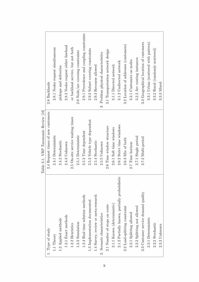
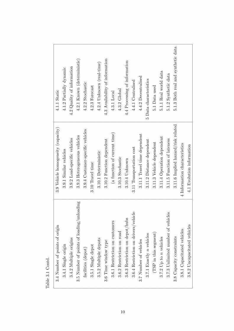
A VRP taxonomic review has been compiled recently [18] and is shown in Table
3.1. Broadly, there are five classifications, these being type of study, scenario char-
acteristics, problem physical characteristics, information characteristics and data
characteristics. The variety of attributes that can be encompassed in a VRP, and
the possibility for subtle differences between problems, is evident.
When comparing the research to be presented in this thesis with other VRP work
7
(Table 3.1), it is notable that the work in this thesis addresses relatively under-
researched areas including real-world problems, directed network, multiple origins,
and multiple depots.
The airline taxi problem or dial-a-flight problem (DAFP) can best be classified
under the PDP class of problems. It differs from the DARP in that passengers
can only start and end their journeys at a limited number of pre-specified locations
(airports), and not at any point on the network. This difference implies that in
the DARP, passengers or passenger groups are unlikely to have origin or destination
locations matching those of any other passenger groups, whereas in the DAFP,
different passengers are likely to have matching locations for origin and destination.
In practical or real world problems, there are a number of often subtle differences
between different situations and these make generalised modelling methods difficult
to devise, even between problems which are apparently of the same type.
Exact methods mostly refer to large-scale integer linear programming problems
(ILPs) and can be difficult to solve. Hasle and Kloster [19] suggest instances of
50-100 bookings cannot be solved consistently using exact methods. This is the
reason both heuristics and metaheuristics are of such widespread interest.
8
Tab
le3.
1:V
RP
Tax
onom
icR
evie
w[1
8]
1.
Typ
eof
stu
dy
2.4
Req
ues
tti
mes
ofn
ewcu
stom
ers
2.8
Back
hau
ls
1.1
Th
eory
2.4.
1D
eter
min
isti
c2.
8.1
Nod
esre
qu
est
sim
ult
an
eou
s
1.2
Ap
pli
edm
eth
od
s2.
4.2
Sto
chas
tic
pic
ku
ps
and
del
iver
ies
1.2
.1E
xac
tm
eth
od
s2.
4.3
Un
kn
own
2.8.2
Nod
esre
qu
est
eith
erli
neh
au
l
1.2
.2H
euri
stic
s2.
5O
n-s
ite
serv
ice
wai
tin
gti
mes
orb
ack
hau
lse
rvic
e,b
ut
not
both
1.2
.3S
imu
lati
on
2.5.
1D
eter
min
isti
c2.
9N
od
e/ar
cco
veri
ng
con
stra
ints
1.2
.4R
eal
tim
eso
luti
onm
eth
od
s2.
5.2
Tim
ed
epen
den
t2.
9.1
Pre
ced
ence
an
dco
up
lin
gco
nst
rain
ts
1.3
Imp
lem
enta
tion
docu
men
ted
2.5.
3V
ehic
lety
pe
dep
end
ent
2.9.2
Su
bse
tco
veri
ng
con
stra
ints
1.4
Su
rvey
,re
vie
wor
met
a-r
esea
rch
2.5.
4S
toch
asti
c2.
9.3
Rec
ou
rse
all
owed
2.
Sce
nar
ioch
ara
cter
isti
cs2.
5.5
Un
kn
own
3.
Pro
ble
mp
hysi
cal
chara
cter
isti
cs
2.1
Nu
mb
erof
stop
son
route
2.6
Tim
ew
ind
owst
ruct
ure
3.1
Tra
nsp
ort
ati
on
net
work
des
ign
2.1
.1K
now
n(d
eter
min
isti
c)2.
6.1
Sof
tti
me
win
dow
s3.
1.1
Dir
ecte
dn
etw
ork
2.1
.2P
art
iall
ykn
own
,p
arti
all
yp
rob
abil
isti
c2.
6.2
Str
ict
tim
ew
ind
ows
3.1.2
Un
dir
ecte
dnet
work
2.2
Loa
d-s
pli
ttin
gco
nst
rain
t2.
6.3
Mix
ofb
oth
3.2
Loca
tion
of
ad
dre
sses
(cu
stom
ers)
2.2
.1S
pli
ttin
gal
low
ed2.
7T
ime
hor
izon
3.2.1
Cu
stom
ers
on
nod
es
2.2
.2S
pli
ttin
gn
ot
all
owed
2.7.
1S
ingl
ep
erio
d3.
2.2
Arc
rou
tin
gin
stan
ces
2.3
Cu
stom
erse
rvic
ed
eman
dqu
ali
ty2.
7.2
Mu
lti-
per
iod
3.3
Geo
gra
ph
ical
loca
tion
of
cust
om
ers
2.3
.1D
eter
min
isti
c3.
3.1
Urb
an(s
catt
ered
wit
hp
att
ern
)
2.3
.2S
toch
asti
c3.
3.2
Ru
ral
(ran
dom
lysc
att
ered
)
2.3
.3U
nkn
own
3.3.3
Mix
ed
9
Tab
le3.1
Con
td.
3.4
Nu
mb
erof
poin
tsof
ori
gin
3.9
Veh
icle
hom
ogen
eity
(cap
acit
y)
4.1.1
Sta
tic
3.4.1
Sin
gle
orig
in3.
9.1
Sim
ilar
veh
icle
s4.
1.2
Part
iall
yd
yn
am
ic
3.4.2
Mu
ltip
leori
gin
s3.
9.2
Loa
d-s
pec
ific
veh
icle
s4.2
Qu
ali
tyof
info
rmati
on
3.5
Nu
mb
erof
poin
tsof
load
ing/u
nlo
adin
g3.
9.3
Het
erog
eneo
us
veh
icle
s4.
2.1
Kn
own
(det
erm
inis
tic)
faci
liti
es(d
epot)
3.9.
4C
ust
omer
-sp
ecifi
cve
hic
les
4.2.2
Sto
chast
ic
3.5.1
Sin
gle
dep
ot3.
10T
rave
lti
me
4.2.3
Fore
cast
3.5.2
Mu
ltip
ledep
ots
3.10
.1D
eter
min
isti
c4.
2.4
Un
kn
own
(rea
l-ti
me)
3.6
Tim
ew
ind
owty
pe
3.10
.2F
un
ctio
nd
epen
den
t4.3
Ava
ilab
ilit
yof
info
rmati
on
3.6.1
Res
tric
tion
on
cust
omer
s(a
fun
ctio
nof
curr
ent
tim
e)4.
3.1
Loca
l
3.6.2
Res
tric
tion
on
road
3.10
.3S
toch
asti
c4.
3.2
Glo
bal
3.6.3
Res
tric
tion
on
dep
ot/
hu
bs
3.10
.4U
nkn
own
4.4
Pro
cess
ing
of
info
rmati
on
3.6.4
Res
tric
tion
on
dri
vers
/ve
hic
le3.
11T
ran
spor
tati
onco
st4.
4.1
Cen
trali
sed
3.7
Nu
mb
erof
veh
icle
s3.
11.1
Tra
vel
tim
ed
epen
den
t4.
4.2
Dec
entr
alise
d
3.7.1
Exact
lyn
veh
icle
s3.
11.2
Dis
tan
ced
epen
den
t5
Dat
ach
ara
cter
isti
cs
(TS
Pin
this
segm
ent)
3.11
.3V
ehic
led
epen
den
t5.
1D
ata
use
d
3.7.2
Up
ton
veh
icle
s3.
11.4
Op
erat
ion
dep
end
ent
5.1.1
Rea
lw
orl
dd
ata
3.7.3
Un
lim
ited
nu
mb
erof
veh
icle
s3.
11.5
Fu
nct
ion
ofla
ten
ess
5.1.2
Synth
etic
data
3.8
Cap
acit
yco
nst
rain
ts3.
11.6
Imp
lied
haz
ard
/ris
kre
late
d5.
1.3
Both
real
an
dsy
nth
etic
data
3.8.1
Cap
acit
ate
dve
hic
les
4In
form
atio
nch
arac
teri
stic
s
3.8.2
Un
cap
acit
ate
dve
hic
les
4.1
Evo
luti
onin
form
atio
n
10
3.1.2 Solving VRPs
Heuristics
Classifications Heuristics are common-sense methods to reduce the size of prob-
lems by, for example, removing variables from a problem. As such they are commonly
used on their own or in conjunction with other methods forNP -hard problems. They
can be classified as construction, improving, mathematical or practical types.
Construction heuristics are applied when constructing the problem (i.e. assembling
the variables and constraints) to achieve a first, feasible solution. In contrast, im-
proving heuristics are applied to an existing solution to improve it.
Mathematical heuristics relate to mathematical manipulations of the formulation.
They are those heuristics suggested by a numerical examination of the problem, for
example, in a maximization problem paying more attention to the variables with
relatively larger objective function coefficients, or lower costs, as is done in column
generation. Preprocessing done by ILP solvers such as implementing cutting planes
(cuts/extra constraints to reduce the feasible region) is another example.
Practical heuristics relate to practical evaluations of the problem setting or envi-
ronment, and removal of obviously impossible or unlikely solutions. They involve
reducing the problem size by specifically eliminating variables which are likely to be
zero in practice. For example, in a scheduling problem, eliminate routes (variables)
which are comparatively long and expensive. Another example is a valid inequality,
which is a cut/additional constraint designed for the problem at hand to decrease
the size of the search region.
Heuristic methods can be applied when using mathematical programming tech-
niques. For example, an iterative method could proceed as follows:
• Formulate an easy to solve relaxed problem by removing some constraints.
• Adjust the problem such that it satisfies the dropped restrictions, or add some
restrictions, and solve the problem again.
• Repeat until an acceptable, feasible solution is obtained.
Heuristics are useful in conjunction with other techniques since they can reduce the
size of a problem substantially. However, since they eliminate possible solutions they
11
need to be carefully considered. Often useful heuristics can be developed which are
specific to a certain problem or problem type.
The best solution procedures are specific to variable types. For example, problems
with only continuous variables can be efficiently solved using the simplex method,
and special techniques exist for efficiently solving purely binary variable problems
[20,21]. Also, numerical heuristic techniques such as Feaspump [22] often work well
for general integer variables and less well for binary variables, so much so that the
latest version works in two phases, first dealing with the binary variables and then
the integer variables. Benders decomposition [23] exploits structure by decomposing
the problem by variable type, i.e. the subproblem is purely binary or purely general
integer.
Construction Heuristics Algorithms Aronson [16] has listed some of the main
construction heuristics for the VRP. An obvious one is the greedy or nearest neigh-
bour algorithm [7] used for the TSP, where the closest neighbour is always the one
travelled to next. Another, related method involves finding and converting minimum
spanning trees (MSTs) into feasible routes [24].
A nearest neighbour algorithm for the VRPTW is described by Solomon [25]. Solomon
uses a distance measure consisting of both geographic and temporal measures of dis-
tance in his algorithm. This distance is given by cij = w1dij +w2Tij +w3vij , where
dij is the geographical distance between two customers, Tij is the time difference
between the completion of the service at i and the start of service at j, and vij is the
urgency of servicing customer j. This urgency is calculated as the time remaining
until the deadline of servicing customer j is reached. w1, w2 and w3 are weights
which when summed together add up to 1.
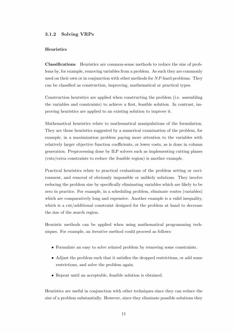
Hosny [26] describes the construction procedure as follows: A route is created with
one customer. Thereafter, customers are inserted sequentially into the route until
no further insertions can feasibly occur. With reference to Figure 3.1, unrouted
customer k is inserted between customers i and j. Insertions are done based on the
time-modified distance measure.
Subtour patching [16] or insertion procedures [7] for a TSP involve creating a number
of subtours, i.e. solving a relaxed version of the TSP without the subtour elimination
constraints. The subtours are then merged (patched) into one cycle. The most
common insertion heuristic is termed the nearest neighbour insertion algorithm [7].
This proceeds in two steps. It first takes a subtour of nodes and finds a node which
12
Figure 3.1: An Insertion Heuristic [26]
should join the subtour next (selection step), then determines where in the subtour
it should be inserted (insertion step).
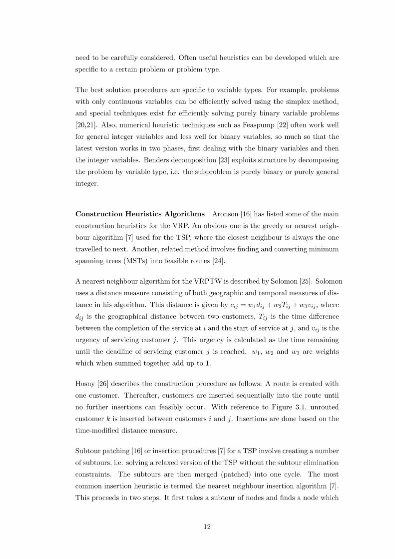
The savings algorithm is a classic algorithm described by Clarke and Wright [27] for
the VRPTW and involves computing the savings (typically in distance) by adding
nodes to a subtour, then selecting the largest saving node and adding it to the
subtour. Initially, each customer is assigned to one vehicle. Thereafter, the savings
achieved by combining two such routes, i.e. taking one such customer i and adding
that customer to the route of another customer j will result in a savings in cost of
Sij = cio + coj − cij , as depicted in Figure 3.2
Figure 3.2: A Savings Heuristic [26]
Two types of construction heuristics are defined by Hosny [26]. These are sequential
construction where routes are constructed after each other, and parallel construction
13
where routes are constructed at the same time. The parallel version of the savings
algorithm involves finding the highest saving among all the customers and executing
that change. The sequential version considers one route at a time and implements
the best saving by joining another route to it.
The nearest merger algorithm involves setting up a number of subtours which are
then merged in a way to reduce costs.
Two-phase algorithms [7,16] are often applied to VRPs. They involve a clustering
phase followed by a routing phase. In these methods, each city is assigned to a
vehicle, and the TSPs are solved for each vehicle-cluster combination. For example,
in the sweep algorithm [28], nodes are first assigned to vehicles, then the order of
visitation is assigned. Customers are represented by their polar coordinates [29].
An angle of 0 is assigned to an arbitrary customer and all other customers’ angles
calculated relative to that and ranked. The procedure is then:
• Choose an unused vehicle.
• Start from the next customer having the smallest angle, and assign customers
to the vehicle until its capacity is reached.
• Optimize each vehicle route using a TSP method.
• Perform vertex exchanges between routes if cost is reduced and re-optimise.
The Fisher and Jaikumar algorithm [30] does the clustering, then uses a TSP to do
the routing for each vehicle. A general assignment problem (GAP) is solved to assign
customers to vehicles. Thereafter a travelling salesperson problem (TSP) with time
windows is solved to optimise the vehicles’ routes. The method is applied to VRPs
from 50 to 199 customers.
Hierarchical cycling involves clustering first into clusters no bigger than some pa-
rameter, then replacing each cluster with a representative node. The new nodes
are clustered in the same way, until only one cluster remains. The node is replaced
with its cluster and the shortest path through the cluster is found. The process is
repeated.
Route first/cluster second algorithms [16] involve constructing a TSP tour for all
nodes except the depot, then breaking the tour into pieces such that all pieces can
be assigned to a vehicle.
14
Many of the heuristics for the multi-vehicle DARP (MVDARP) are two-phase algo-
rithms in which phase 1 selects and clusters users and phase 2 routes the vehicles.
Dumas et al. [31] proposed creating mini-clusters of customers, where each mini-
cluster is transportable by one vehicle, while respecting time constraints, vehicle
capacity, pairing and precedence. The mini-clusters are combined to form feasible
routes using column generation. Ioachim et al. [32] showed that an optimisation
technique in the clustering phase is advantageous.
Improving Heuristics Algorithms These involve taking a solution and search-
ing for improving modifications, often iteratively. A feasible solution must first be
found using a construction method. Then, for example, a search will be conducted
among neighbouring solutions for an improved one. The definition of the neigh-
bourhood defines how the search is conducted. For example, a savings/insertion
algorithm quickly finds an initial solution, sometimes by creating many routes with
only one customer, then improves it towards a cheaper solution. This is done by
merging routes together as long as this process saves costs.
If a reduced cost solution is found it may be adopted if the first acceptance criteria
is used [26]. Otherwise, if using the best acceptance criteria, all the neighbourhood
solutions are evaluated first and the best is chosen to be implemented.
A local search involves finding a new solution in the neighbourhood of the current
solution [26]. Care must be taken to avoid local optima which is why techniques such
as tabu search are used. The neighbourhood size can be varied. If it is increased
it becomes a large neighbourhood search (LNS) method. Variable neighbourhood
search (VNS) has been suggested by Hansen and Mladenovic [33]. This involves
gradually increasing the neighbourhood size until a stopping condition is met. VNS
has been successfully applied to a number of VRPs, for example, the VRPTW [34],
the PD travelling salesperson problem (PDTSP) [35], the periodic VRPTW [36] and
the multi-depot VRPTW [37]). It was hybridised with simulated annealing (SA) to
solve the PDP by Hosny [26].
Improvement/exchange algorithms involve finding an initial solution, then improv-
ing/exchanging edges, nodes and/or vehicles to find improvements (edges are some-
times also referred to as links, arcs or legs in a routing network). The most common
are the k-optimal methods involving the deletion of k edges and replacement by k
other edges. 2-opt and 3-opt versions are most common, since using more edges typ-
ically expands the neighbourhood too much and involves too many options, making
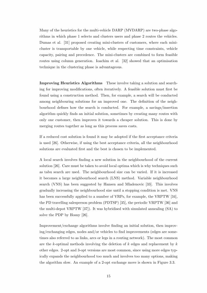
the algorithm slow. An example of a 2-opt exchange move is shown in Figure 3.3.
15
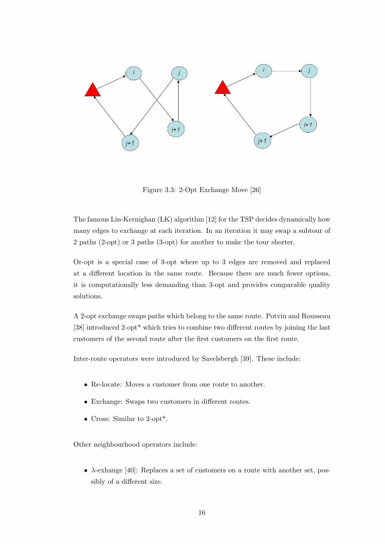
Figure 3.3: 2-Opt Exchange Move [26]
The famous Lin-Kernighan (LK) algorithm [12] for the TSP decides dynamically how
many edges to exchange at each iteration. In an iteration it may swap a subtour of
2 paths (2-opt) or 3 paths (3-opt) for another to make the tour shorter.
Or-opt is a special case of 3-opt where up to 3 edges are removed and replaced
at a different location in the same route. Because there are much fewer options,
it is computationally less demanding than 3-opt and provides comparable quality
solutions.
A 2-opt exchange swaps paths which belong to the same route. Potvin and Rousseau
[38] introduced 2-opt* which tries to combine two different routes by joining the last
customers of the second route after the first customers on the first route.
Inter-route operators were introduced by Savelsbergh [39]. These include:
• Re-locate: Moves a customer from one route to another.
• Exchange: Swaps two customers in different routes.
• Cross: Similar to 2-opt*.
Other neighbourhood operators include:
• λ-exhange [40]: Replaces a set of customers on a route with another set, pos-
sibly of a different size.
16

• CROSS-exchange [41]: Swaps two groups of customers from one route to an-
other.
• GENI-exchange [42]: An extension of the re-locate operator to allow for cus-
tomer insertion between non-consecutive customers on another route.
• Ejection chains [43]: Exchange of customer sets, but operates on more than
two routes.
• Cyclic k-transfers [44]: Transfer of customers from one route to another.
• Modified ejection chains [45]: Includes re-ordering of routes.
Most heuristic methods are specific to a certain type of problem. Pisinger and Ropke
[46] describe a heuristic which can solve five variants of the VRP; the vehicle routing
problem with time windows (VRPTW), the capacitated vehicle routing problem
(CVRP), the multi-depot VRP (MDVRP), the site-dependant VRP (SDVRP) and
the open VRP (OVRP). An adaptive large neighbourhood search (ALNS) framework
is described which involves a number of simple, fast algorithms competing to modify
the current solution. Each iteration involves choosing an algorithm to destroy the
current solution and then choosing an algorithm to repair the solution.
Large neighbourhood search (LNS) algorithms [15] might remove and replace a large
number of customers (30% - 40%) in an iteration. They are computationally more
expensive than faster, simpler algorithms but can provide good results [47] [46]. It
has been suggested that the success of neighbourhood search algorithms obviates the
need for sophisticated construction algorithms which are generally time consuming,
parameter dependent and hard to implement [15].
Metaheuristics Metaheuristics have become popular for VRPs because they al-
low smaller, non-linear and discrete variable model formulations, at the expense
of slow processing and convergence. Genetic algorithms (GA), tabu search (TS),
particle swarm optimization (PSO), ant colony optimization (ACO) and simulated
annealing (SA) have been applied to vehicle transport scheduling problems.
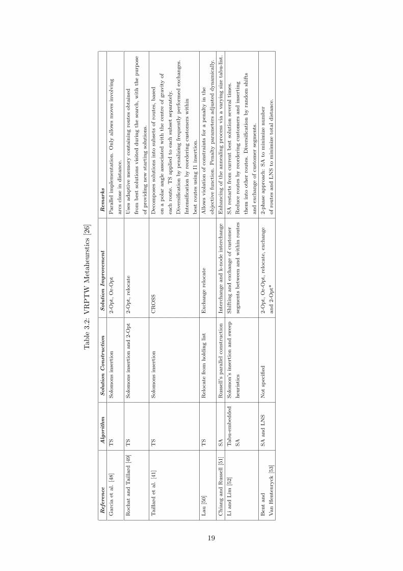
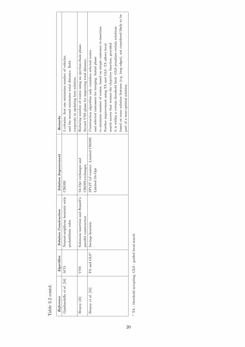
A summary of metaheuristic techniques for the VRPTW is shown in Table 3.2[26].
Practitioners often apply a cheapest insertion method for initial feasible solution
construction such as that proposed by Solomon [25]. Solomon’s I1 insertion heuristic
starts by initialising a route, then inserts a new customer between two others in
the route. The cost of insertion is minimised while retaining feasibility. Solution
improvement generally uses a k-opt method. Heuristics are designed for the specific
17

problem to reduce the search area. Specifically, Garcia et al. [48] only allow inclusion
of the relatively shorter edges.
18
Tab
le3.
2:V
RP
TW
Met
aheu
rsti
cs[2
6]
Refe
ren
ceA
lgori
thm
Solu
tion
Con
stru
cti
on
Solu
tion
Impro
vem
en
tR
em
ark
s
Garc
iaet
al.
[48]
TS
Solo
mon
sin
sert
ion
2-O
pt,
Or-
Op
tP
ara
llel
imp
lem
enta
tion
.O
nly
allow
sm
oves
involv
ing
arc
scl
ose
ind
ista
nce
.
Roch
at
an
dT
ailla
rd[4
9]
TS
Solo
mon
sin
sert
ion
an
d2-O
pt
2-O
pt,
relo
cate
Use
sad
ap
tive
mem
ory
conta
inin
gro
ute
sob
tain
ed
from
bes
tso
luti
on
svis
ited
du
rin
gth
ese
arc
h,
wit
hth
ep
urp
ose
of
pro
vid
ing
new
start
ing
solu
tion
s.
Tailla
rdet
al.
[41]
TS
Solo
mon
sin
sert
ion
CR
OS
SD
ecom
pose
sso
luti
on
sin
tosu
bse
tsof
rou
tes,
base
d
on
ap
ola
ran
gle
ass
oci
ate
dw
ith
the
centr
eof
gra
vit
yof
each
rou
te.
TS
ap
plied
toea
chsu
bse
tse
para
tely
.
Div
ersi
fica
tion
by
pen
alizi
ng
freq
uen
tly
per
form
edex
chan
ges
.
Inte
nsi
fica
tion
by
reord
erin
gcu
stom
ers
wit
hin
bes
tro
ute
su
sin
gI1
inse
rtio
n.
Lau
[50]
TS
Rel
oca
tefr
om
hold
ing
list
Exch
an
ge
relo
cate
Allow
svio
lati
on
of
con
stra
ints
for
ap
enalt
yin
the
ob
ject
ive
fun
ctio
n.
Pen
alt
yp
ara
met
ers
ad
just
edd
yn
am
ically.
Ch
ian
gan
dR
uss
ell
[51]
SA
Ru
ssel
l’s
para
llel
con
stru
ctio
nIn
terc
han
ge
an
dk-n
od
ein
terc
han
ge
En
han
cin
gof
the
an
nea
lin
gp
roce
ssvia
avary
ing
size
tab
u-l
ist.
Li
an
dL
im[5
2]
Tab
u-e
mb
edd
edS
olo
mon
’sin
sert
ion
an
dsw
eep
Sh
ifti
ng
an
dex
chan
ge
of
cust
om
erS
Are
start
sfr
om
curr
ent
bes
tso
luti
on
sever
al
tim
es.
SA
heu
rist
ics
segm
ents
bet
wee
nan
dw
ith
inro
ute
sR
edu
cero
ute
sby
reord
erin
gcu
stom
ers
an
din
sert
ing
them
into
oth
erro
ute
s.D
iver
sifi
cati
on
by
ran
dom
shif
ts
an
dex
chan
ge
of
cust
om
erse
gm
ents
.
Ben
tan
dS
Aan
dL
NS
Not
spec
ified
2-O
pt,
Or-
Op
t,re
loca
te,
exch
an
ge
2-p
hase
ap
pro
ach
:S
Ato
min
imiz
enu
mb
er
Van
Hen
ten
ryck
[53]
an
d2-O
pt*
of
rou
tes
an
dL
NS
tom
inim
ize
tota
ld
ista
nce
.
19
Tab
le3.
2co
ntd
.
Refe
ren
ceA
lgori
thm
Solu
tion
Con
stru
cti
on
Solu
tion
Impro
vem
en
tR
em
ark
s
Gam
bard
ellaetal.
[54]
AC
ON
eare
st-n
eighb
ou
rh
euri
stic
wit
hC
RO
SS
2co
lon
ies:
firs
ton
em
inim
izes
nu
mb
erof
veh
icle
s,
pro
bab
ilis
tic
rule
san
dth
ese
con
dm
inim
izes
tota
ld
ista
nce
.B
oth
coop
erate
inu
pd
ati
ng
bes
tso
luti
on
.
Bra
ysy
[45]
VN
SS
olo
mon
sin
sert
ion
an
dR
uss
ell’
sO
r-O
pt
exch
an
ges
an
dR
edu
cin
gnu
mb
erof
rou
tes
usi
ng
an
ejec
tion
-ch
ain
ph
ase
.
para
llel
con
stru
ctio
nC
RO
SS
-exch
an
ges
Sec
on
dV
NS
ph
ase
for
imp
rovin
gto
tal
dis
tan
ce.
Bra
ysyetal.
[55]
TA
an
dG
LS∗
Savin
gs
heu
rist
icS
PL
IT(o
fro
ute
s).
Lim
ited
CR
OS
S.
Con
stru
ctio
nalg
ori
thm
on
lyco
nsi
der
sse
lect
edro
ute
s
Lim
ited
Or-
Op
tan
dse
lect
edcu
stom
ers
for
mer
gin
g.
Init
ial
ph
ase
tom
inim
ize
nu
mb
erof
rou
tes,
base
don
sim
ple
cust
om
erre
-in
sert
ion
.
Fu
rth
erim
pro
vem
ent
usi
ng
TA
an
dG
LS
-TA
allow
slo
cal
searc
hm
oves
that
wors
enth
eob
ject
ive
fun
ctio
n,
pro
vid
ed
itis
wit
hin
ace
rtain
thre
shold
lim
it-G
LS
pen
alize
sce
rtain
solu
tion
s
base
don
som
eso
luti
on
featu
res
(e.g
.lo
ng
edges
),n
ot
con
sid
ered
likel
yto
be
part
of
an
ear-
op
tim
al
solu
tion
.
∗T
A-
thre
shold
acc
epti
ng,
GL
S-
gu
ided
loca
lse
arc
h
20
Simulated annealing (SA) is a search procedure successfully applied to various VRPs
including those devised by Osman [40]. Nanry and Barnes [56], Cordeau and Laporte
[8] and Gendreau et al. [57] apply tabu search for the multiple VRP with pickup and
delivery (VRPPD), DARP and urban courier service problems (UCSP) respectively.
Cordeau and Laporte [58] state that tabu search is the most successful metaheuristic
for the VRP, having outperformed alternative methods in a number of benchmark
studies.
Ant colony optimization (ACO) has been applied to certain VRPs such as the
VRPPD [59,60], the CVRP [61,62], VRPTW [60], the TSP [63] and the standard
VRP [64]. It has not been applied to the MVCVRP or MVCVRPTW, since there
appear to be issues dealing with the multi-vehicle constraint.
Like most metaheuristics, ACO can be adjusted in various ways for a specific prob-
lem. Gambardella et al. [54] used it to solve the VRPTW and use global pheromone
updating, as opposed to the more usual local updating.
Hybrid metaheuristics refer to combining two or more methods and have become
popular for VRPs. A taxonomy of such methods has been presented by Talbi [65].
Hybridisations can be classified according to whether the different methods occur
sequentially (relay) or whether agents are parallel (or teamwork/cooperating). Lo-
cal optimisations can be carried out by different metaheuristics (low-level), or the
metaheuristic for the global optimisation (high-level) could be varied. Methods can
include deterministic methods such as ILPs and often heuristic methods are also
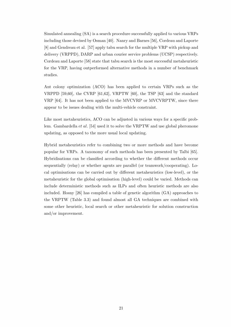
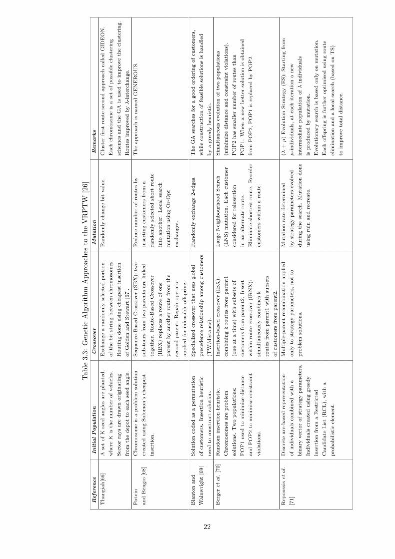
included. Hosny [26] has compiled a table of genetic algorithm (GA) approaches to
the VRPTW (Table 3.3) and found almost all GA techniques are combined with
some other heuristic, local search or other metaheuristic for solution construction
and/or improvement.
21
Tab
le3.3
:G
enet
icA
lgor
ith
mA
pp
roac
hes
toth
eV
RP
TW
[26]
Refe
ren
ceIn
itia
lP
opu
lati
on
Cro
ssover
Mu
tati
on
Rem
ark
s
Th
an
gia
h[6
6]
Ase
tof
Kse
edan
gle
sare
pla
nte
d,
Exch
an
ge
ara
nd
om
lyse
lect
edp
ort
ion
Ran
dom
lych
an
ge
bit
valu
e.C
lust
erfi
rst
rou
tese
con
dap
pro
ach
called
GID
EO
N.
wh
ere
Kis
the
nu
mb
erof
veh
icle
s.of
the
bit
stri
ng
bet
wee
nch
rom
oso
mes
Each
chro
moso
me
isa
set
of
poss
ible
clu
ster
ing
Sec
tor
rays
are
dra
wn
ori
gin
ati
ng
Rou
tin
gd
on
eu
sin
gch
eap
est
inse
rtio
nsc
hem
esan
dth
eG
Ais
use
dto
imp
rove
the
clu
ster
ing.
from
the
dep
ot
toea
chse
edan
gle
.of
Gold
enan
dS
tew
art
[67].
Rou
tes
imp
roved
byλ
-inte
rch
an
ge.
Potv
inC
hro
moso
me
isa
pro
ble
mso
luti
on
Seq
uen
ce-B
ase
dC
ross
over
(SB
X):
two
Red
uce
nu
mb
erof
rou
tes
by
Th
eap
pro
ach
isn
am
edG
EN
ER
OU
S.
an
dB
engio
[68]
crea
ted
usi
ng
Solo
mon
’sch
eap
est
sub
-tou
rsfr
om
two
pare
nts
are
lin
ked
inse
rtin
gcu
stom
ers
from
a
inse
rtio
n.
toget
her
.R
ou
te-B
ase
dC
ross
over
ran
dom
lyse
lect
edsh
ort
rou
te
(RB
X)
rep
lace
sa
rou
teof
on
ein
toan
oth
er.
Loca
lse
arc
h
pare
nt
by
an
oth
erro
ute
from
the
muta
tion
usi
ng
Or-
Op
t
seco
nd
pare
nt.
Rep
air
op
erato
rex
chan
ges
.
ap
plied
for
infe
asi
ble
off
spri
ng.
Bla
nto
nan
dS
olu
tion
cod
edas
ap
erm
uta
tion
Sp
ecia
lize
dcr
oss
over
that
use
sglo
bal
Ran
dom
lyex
chan
ge
2-e
dges
.T
he
GA
searc
hes
for
agood
ord
erin
gof
cust
om
ers,
Wain
wri
ght
[69]
of
cust
om
ers.
Inse
rtio
nh
euri
stic
pre
ced
ence
rela
tion
ship
am
on
gcu
stom
ers
wh
ile
con
stru
ctio
nof
feasi
ble
solu
tion
sis
han
dle
d
use
dto
con
stru
ctso
luti
on
.(T
W/d
ista
nce
).by
agre
edy
heu
rist
ic.
Ber
geretal.
[70]
Ran
dom
inse
rtio
nh
euri
stic
.In
sert
ion
-base
dcr
oss
over
(IB
X):
Larg
eN
eighb
ou
rhood
Sea
rch
Sim
ult
an
eou
sev
olu
tion
of
two
pop
ula
tion
s
Ch
rom
oso
mes
are
pro
ble
mco
mb
inin
gk
rou
tes
from
pare
nt1
(LN
S)
mu
tati
on
.E
ach
cust
om
er(m
inim
ize
dis
tan
cean
dco
nst
rain
tvio
lati
on
s).
solu
tion
s.T
wo
pop
ula
tion
s:(o
ne
at
ati
me)
wit
hsu
bse
tsof
con
sid
ered
for
rein
sert
ion
PO
P2
has
smaller
nu
mb
erof
rou
tes
than
PO
P1
use
dto
min
imiz
ed
ista
nce
cust
om
ers
from
pare
nt2
.In
sert
inan
alt
ern
ate
rou
te.
PO
P1.
Wh
ena
new
bet
ter
solu
tion
isob
tain
ed
an
dP
OP
2to
min
imis
eco
nst
rain
tw
ith
inro
ute
cross
over
(IR
NX
):E
lim
inate
short
est
rou
te.
Reo
rder
from
PO
P2,
PO
P1
isre
pla
ced
by
PO
P2.
vio
lati
on
s.si
mu
ltan
eou
sly
com
bin
esk
cust
om
ers
wit
hin
aro
ute
.
rou
tes
from
pare
nt1
wit
hsu
bse
ts
of
cust
om
ers
from
pare
nt2
.
Rep
ou
ssisetal.
Dis
cret
earc
-base
dre
pre
senta
tion
Mu
ltip
le-p
are
nt
reco
mb
inati
on
ap
plied
Mu
tati
on
rate
det
erm
ined
(λ+µ
)E
volu
tion
Str
ate
gy
(ES
):S
tart
ing
from
[71]
of
ind
ivid
uals
com
bin
edw
ith
aon
lyto
stra
tegy
para
met
ers,
not
toby
stra
tegy
para
met
ers
evolv
edµ
-in
div
idu
als
,at
each
iter
ati
on
an
ew
bin
ary
vec
tor
of
stra
tegy
para
met
ers.
pro
ble
mso
luti
on
s.d
uri
ng
the
searc
h.
Mu
tati
on
don
ein
term
edia
tep
op
ula
tion
ofλ
ind
ivid
uals
Ind
ivid
uals
crea
ted
usi
ng
gre
edy
usi
ng
ruin
an
dre
crea
te.
isp
rod
uce
dby
mu
tati
on
.
inse
rtio
nfr
om
aR
estr
icte
dE
volu
tion
ary
searc
his
base
don
lyon
mu
tati
on
.
Can
did
ate
Lis
t(R
CL
),w
ith
aE
ach
off
spri
ng
isfu
rth
erop
tim
ised
usi
ng
rou
te
pro
bab
ilis
tic
elem
ent.
elim
inati
on
an
da
loca
lse
arc
h(b
ase
don
TS
)
toim
pro
ve
tota
ld
ista
nce
.
22
The “ants” in ACO schemes could be termed “agents” and compared to the use of
intelligent agents in, for example, agent-based simulation (ABS). In fact, ABS has
been successfully used to solve VRPs [72–74].
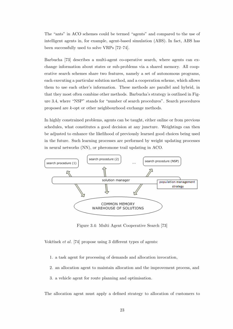
Barbucha [73] describes a multi-agent co-operative search, where agents can ex-
change information about states or sub-problems via a shared memory. All coop-
erative search schemes share two features, namely a set of autonomous programs,
each executing a particular solution method, and a cooperation scheme, which allows
them to use each other’s information. These methods are parallel and hybrid, in
that they most often combine other methods. Barbucha’s strategy is outlined in Fig-
ure 3.4, where “NSP” stands for “number of search procedures”. Search procedures
proposed are k-opt or other neighbourhood exchange methods.
In highly constrained problems, agents can be taught, either online or from previous
schedules, what constitutes a good decision at any juncture. Weightings can then
be adjusted to enhance the likelihood of previously learned good choices being used
in the future. Such learning processes are performed by weight updating processes
in neural networks (NN), or pheromone trail updating in ACO.
Figure 3.4: Multi Agent Cooperative Search [73]
Vokrınek et al. [74] propose using 3 different types of agents:
1. a task agent for processing of demands and allocation invocation,
2. an allocation agent to maintain allocation and the improvement process, and
3. a vehicle agent for route planning and optimisation.
The allocation agent must apply a defined strategy to allocation of customers to
23

routes/vehicles with a cost minimising objective. It works in two phases, an alloca-
tion phase and an improvement phase. The vehicle agent solves a TSP to find the
best route.
Neural networks were employed by Potvin et al. [75] in competitive form to improve
the construction phase of a parallel insertion heuristic for a VRPTW. In another
study [76], neural networks are used in the selection of the best heuristic for a VRP
based on the problem characteristics. Torki et al. [77] describe achieving good results
using a competitive neural network to solve the TSP, the m-TSP and the CVRP.
The TSP normally involves one “salesman” travelling to all the cities. m-TSP is the
version of the TSP with multiple salesmen available to visit the cities.
Pickup and Delivery Problems General PDPs (GPDPs) occur frequently in
practice in areas such as courier services, transportation of raw materials from sup-
pliers to factories, food collection and delivery and newspaper delivery [26]. Parragh
et al. [78] provide a survey and classification of GPDPs as shown in Figure 3.5. The
following acronyms are used [79]:
• VRPB: VRP with backhauls.
• TSPCB: TSP with clustered backhauls.
• VRPCB: VRP with clustered backhauls.
• TSPMB: TSP with mixed linehauls and backhauls
• VRPMB: VRP with mixed linehauls and backhauls.
• TSPDDP: TSP with divisible delivery and pickup.
• VRPDDP: VRP with divisible delivery and pickup.
• TSPSDP: TSP with simultaneous delivery and pickup.
• VRPSDP: VRP with simultaneous delivery and pickup.
• VRPPD: VRP with pickups and deliveries
Some problems have full truckloads and others less than full truckloads. Delivery
locations may be paired where no other customer can be visited in-between. A single
commodity or multiple commodities may be involved, or the problem may involve
the transportation of people.
Important GPDP constraints include [26]:
24
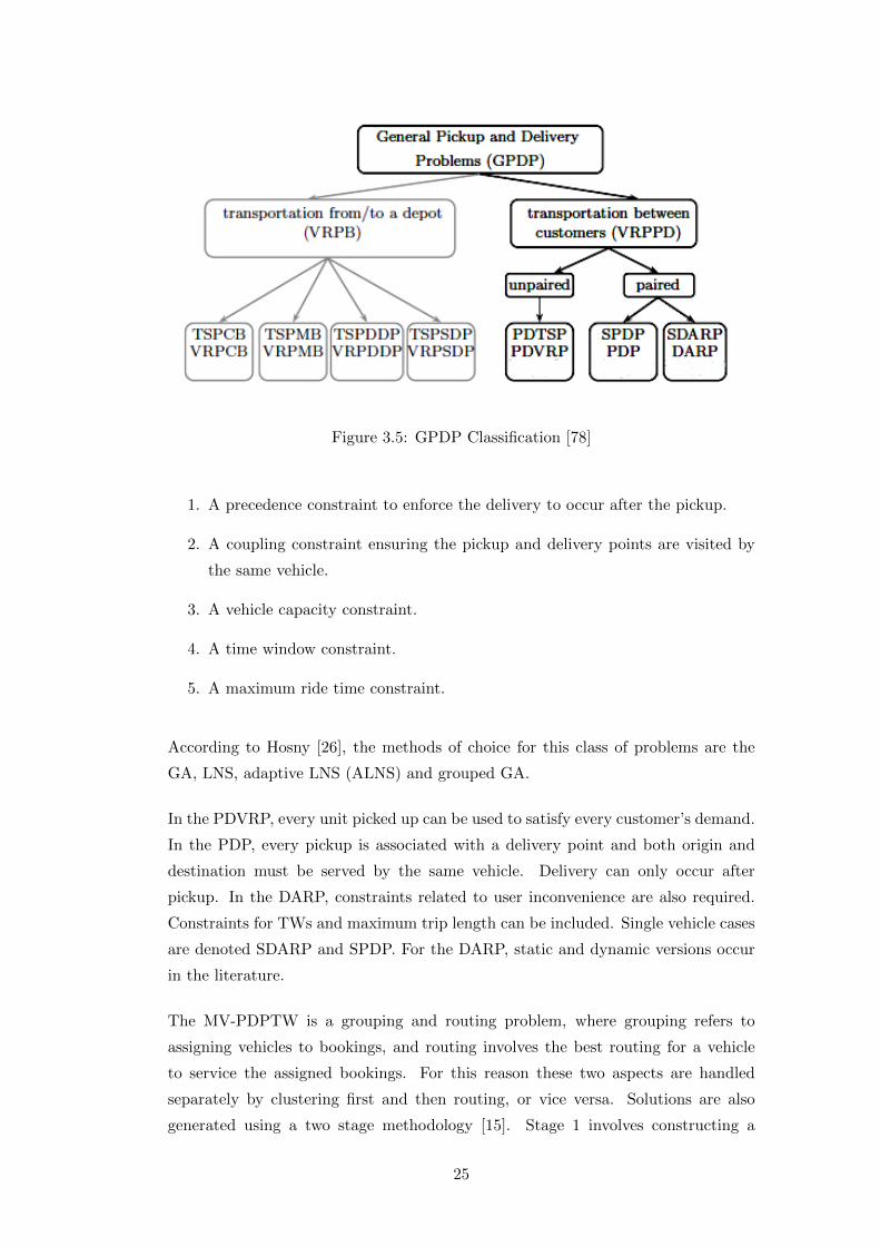
Figure 3.5: GPDP Classification [78]
1. A precedence constraint to enforce the delivery to occur after the pickup.
2. A coupling constraint ensuring the pickup and delivery points are visited by
the same vehicle.
3. A vehicle capacity constraint.
4. A time window constraint.
5. A maximum ride time constraint.
According to Hosny [26], the methods of choice for this class of problems are the
GA, LNS, adaptive LNS (ALNS) and grouped GA.
In the PDVRP, every unit picked up can be used to satisfy every customer’s demand.
In the PDP, every pickup is associated with a delivery point and both origin and
destination must be served by the same vehicle. Delivery can only occur after
pickup. In the DARP, constraints related to user inconvenience are also required.
Constraints for TWs and maximum trip length can be included. Single vehicle cases
are denoted SDARP and SPDP. For the DARP, static and dynamic versions occur
in the literature.
The MV-PDPTW is a grouping and routing problem, where grouping refers to
assigning vehicles to bookings, and routing involves the best routing for a vehicle
to service the assigned bookings. For this reason these two aspects are handled
separately by clustering first and then routing, or vice versa. Solutions are also
generated using a two stage methodology [15]. Stage 1 involves constructing a
25
solution and stage 2 improving the solution. A typical construction methodology is
a least-cost insertion algorithm.
The vehicle routing problem with backhauls (VRPB) involves the transportation of
goods from the depot to customers and vice versa [26]. This type of problem can be
one of four sub-types:
1. Vehicle routing problem with clustered backhauls (VRPCB): All delivery cus-
tomers must be visited after all pickup customers.
2. Vehicle routing problem with mixed linehauls and backhauls (VRPMB): Mixed
visiting of pickup and delivery customers is allowed.
3. Vehicle routing problem with divisible deliver and pickup (VRPDDP): Each
customer is both a pickup and a delivery customer and two visits to the same
customer are allowed.
4. Vehicle routing problem with simultaneous delivery and pickup (VRPSDP):
Each customer requires a pickup and a delivery, but only one visit is allowed.
According to Hosny [26], for this class of problems the large neighbourhood search
algorithm (LNS) is the heuristic of choice.
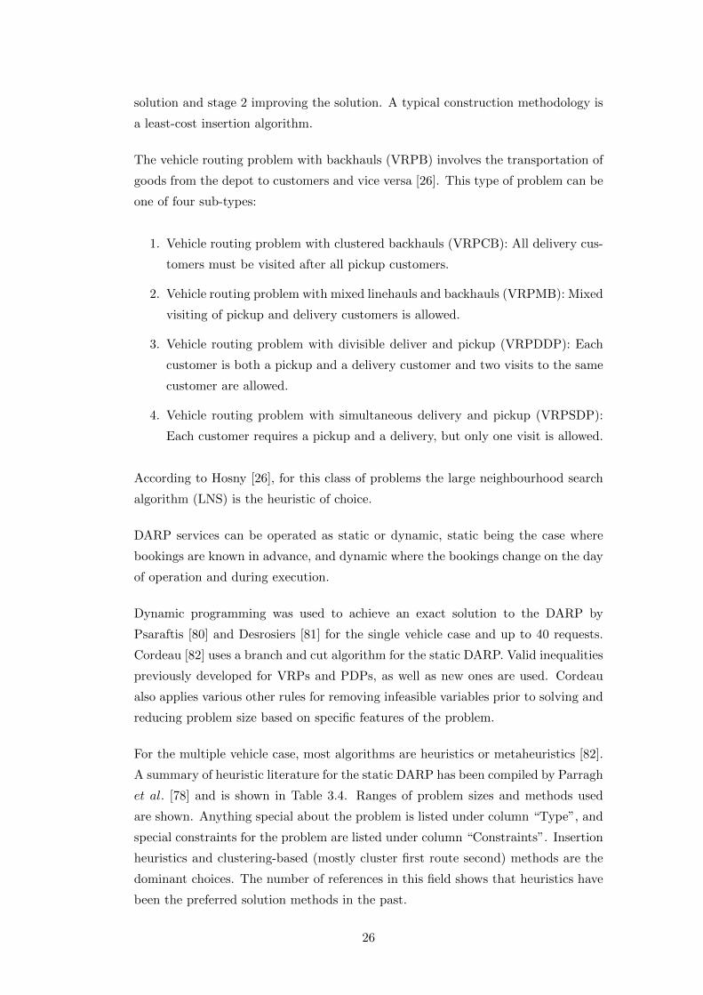
DARP services can be operated as static or dynamic, static being the case where
bookings are known in advance, and dynamic where the bookings change on the day
of operation and during execution.
Dynamic programming was used to achieve an exact solution to the DARP by
Psaraftis [80] and Desrosiers [81] for the single vehicle case and up to 40 requests.
Cordeau [82] uses a branch and cut algorithm for the static DARP. Valid inequalities
previously developed for VRPs and PDPs, as well as new ones are used. Cordeau
also applies various other rules for removing infeasible variables prior to solving and
reducing problem size based on specific features of the problem.
For the multiple vehicle case, most algorithms are heuristics or metaheuristics [82].
A summary of heuristic literature for the static DARP has been compiled by Parragh
et al. [78] and is shown in Table 3.4. Ranges of problem sizes and methods used
are shown. Anything special about the problem is listed under column “Type”, and
special constraints for the problem are listed under column “Constraints”. Insertion
heuristics and clustering-based (mostly cluster first route second) methods are the
dominant choices. The number of references in this field shows that heuristics have
been the preferred solution methods in the past.
26

Tab
le3.
4:D
AR
PH
euri
stic
s[7
8]R
efe
ren
ceT
ype
Obje
cti
ve
Con
stra
ints
Alg
ori
thm
Siz
e
Sin
gle
vehic
leca
se
Psa
raft
is[8
3]
Min
imis
ero
uti
ng
cost
MS
Th
euri
stic
,lo
cal
inte
rch
an
ges
Up
to50
requ
ests
Psa
raft
is[8
4]
Min
imis
ero
uti
ng
cost
Ad
ap
ted
2-o
pt
an
d3-o
pt
Up
to30
requ
ests
Sex
ton
an
dB
od
in[8
5][86]
Min
imis
ecu
stom
erD
esir
edd
eliv
ery
tim
eR
ou
tin
gan
dsc
hed
ulin
galg
ori
thm
Up
to20
requ
ests
inco
nven
ien
ceb
ase
don
Ben
der
’sd
ecom
posi
tion
Hea
lyan
dM
oll
[87]
Min
imis
ero
uti
ng
cost
2-o
pt
imp
rovem
ent,
Up
to100
op
tim
isin
g/sa
crifi
cin
gp
hase
sre
qu
ests
Mu
lti-
vehic
leca
se
Cu
llen
etal.
[88]
Min
imis
ero
uti
ng
cost
sC
lust
erfi
rst,
rou
tese
con
d,
colu
mn
Up
to50
requ
ests
gen
erati
on
Royetal.
[89][90]
Het
erogen
eou
sM
inim
ise
rou
tin
gco
sts,
Tim
ew
ind
ow
sP
ara
llel
inse
rtio
nU
pto
578
flee
tM
inim
ise
cust
om
erre
qu
ests
inco
nven
ien
ce
Bod
inan
dS
exto
n[9
1]
Min
imis
ecu
stom
erD
esir
edd
eliv
ery
tim
eC
lust
erfi
rst,
rou
tese
con
dU
pto
85
requ
ests
inco
nven
ien
ce
Jawetal.
[92]
Min
imis
ero
uti
ng
cost
s,T
ime
win
dow
s,S
equ
enti
al
feasi
ble
inse
rtio
nU
pto
2617
Min
imis
ecu
stom
erri
de
tim
ealg
ori
thm
requ
ests
inco
nven
ien
ce
27
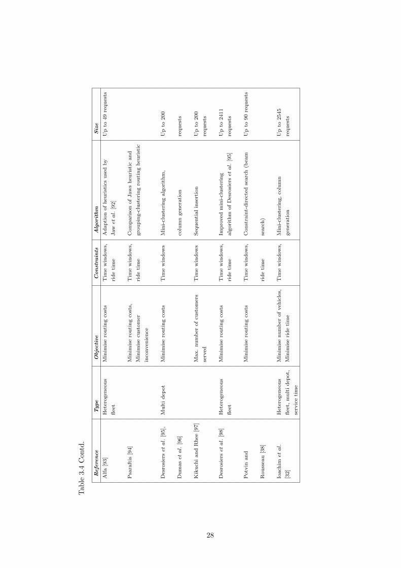
Tab
le3.4
Con
td.
Refe
ren
ceT
ype
Obje
cti
ve
Con
stra
ints
Alg
ori
thm
Siz
e
Alf
a[9
3]
Het
erogen
eou
sM
inim
ise
rou
tin
gco
sts
Tim
ew
ind
ow
s,A
dap
tion
of
heu
rist
ics
use
dby
Up
to49
requ
ests
flee
tri
de
tim
eJawetal.
[92]
Psa
raft
is[9
4]
Min
imis
ero
uti
ng
cost
s,T
ime
win
dow
s,C
om
pari
son
of
Jaw
sh
euri
stic
an
d
Min
imis
ecu
stom
erri
de
tim
egro
up
ing-c
lust
erin
gro
uti
ng
heu
rist
ic
inco
nven
ien
ce
Des
rosi
ersetal.
[95],
Mu
lti
dep
ot
Min
imis
ero
uti
ng
cost
sT
ime
win
dow
sM
ini-
clu
ster
ing
alg
ori
thm
,U
pto
200
Du
masetal.
[96]
colu
mn
gen
erati
on
requ
ests
Kik
uch
ian
dR
hee
[97]
Max.
nu
mb
erof
cust
om
ers
Tim
ew
ind
ow
sS
equ
enti
al
inse
rtio
nU
pto
200
serv
edre
qu
ests
Des
rosi
ersetal.
[98]
Het
erogen
eou
sM
inim
ise
rou
tin
gco
sts
Tim
ew
ind
ow
s,Im
pro
ved
min
i-cl
ust
erin
gU
pto
2411
flee
tri
de
tim
ealg
ori
thm
of
Des
rosi
ersetal.
[95]
requ
ests
Potv
inan
dM
inim
ise
rou
tin
gco
sts
Tim
ew
ind
ow
s,C
on
stra
int-
dir
ecte
dse
arc
h(b
eam
Up
to90
requ
ests
Rou
ssea
u[3
8]
rid
eti
me
searc
h)
Ioach
imetal.
Het
erogen
eou
sM
inim
ise
nu
mb
erof
veh
icle
s,T
ime
win
dow
s,M
ini-
clu
ster
ing,
colu
mn
Up
to2545
[32]
flee
t,m
ult
id
epot,
Min
imis
eri
de
tim
egen
erati
on
requ
ests
serv
ice
tim
e
28

Tab
le3.4
Con
td.
Refe
ren
ceT
ype
Obje
cti
ve
Con
stra
ints
Alg
ori
thm
Siz
e
Mad
senetal.
Het
erogen
eou
sM
inim
ise
rou
tin
gco
st,
Tim
ew
ind
ow
s,R
EB
US
inse
rtio
nb
ase
dU
pto
300
[99]
flee
t,m
inim
ise
nu
mb
erof
veh
icle
s,ri
de
tim
e,ro
ute
alg
ori
thm
requ
ests
serv
ice
tim
em
inim
ise
tota
lw
ait
ing
tim
e,d
ura
tion
min
imis
ed
evia
tion
from
pro
mis
edse
rvic
e
Toth
an
dV
igo
[100]
Het
erogen
eou
sM
inim
ise
rou
tin
gco
st,
Tim
ew
ind
ow
s,P
ara
llel
inse
rtio
n,
imp
roved
by
flee
tri
de
tim
etr
ipin
sert
ion
,ex
chan
ge,
dou
ble
inse
rtio
nm
oves
Born
dorf
erH
eter
ogen
eou
sM
inim
ise
rou
tin
gco
stT
ime
win
dow
s,C
lust
erfi
rst
rou
tese
con
d,
set
Up
to1771
etal.
[101]
flee
t,m
ult
id
epot,
rou
ted
ura
tion
,p
art
itio
nin
g,
bra
nch
an
db
ou
nd
requ
ests
serv
ice
tim
e(r
ide
tim
e)
Fu
[102]
Het
erogen
eou
sM
inim
ise
rou
tin
gco
st,
Tim
ew
ind
ow
s,P
ara
llel
inse
rtio
n,
stoch
ast
ictr
avel
Up
to2800
flee
t,se
rvic
eM
inim
ise
cust
om
erri
de
tim
eti
mes
requ
ests
tim
ein
conven
ien
ce
Dia
na
an
dM
inim
ise
rou
tin
gco
st,
Tim
ew
ind
ow
s,P
ara
llel
regre
tin
sert
ion
heu
rist
icU
pto
1000
Des
sou
ky
[103]
Min
imis
ecu
stom
erri
de
tim
ere
qu
ests
inco
nven
ien
ce,
min
imis
eid
leti
mes
Xia
ng
etal.
Het
erogen
eou
sM
inim
ise
rou
tin
gco
st,
Tim
ew
ind
ow
s,C
on
stru
ctio
nim
pro
vem
ent;
Up
to150
[104]
flee
t,se
rvic
eri
de
tim
e,cl
ust
erin
gby
tim
ew
ind
ow
s,id
eas
of
swee
pre
qu
ests
tim
ero
ute
du
rati
on
,h
euri
stic
s,lo
cal
searc
him
pro
vem
ent
bre
ak
tim
eb
etw
een
trip
s
29

Tab
le3.4
Con
td.
Refe
ren
ceT
ype
Obje
cti
ve
Con
stra
ints
Alg
ori
thm
Siz
e
Won
gan
dB
ell
Het
erogen
eou
sM
inim
ise
rou
tin
gco
st,
Tim
ew
ind
ow
s,P
ara
llel
inse
rtio
n,
imp
roved
by
trip
Up
to150
[105]
flee
t,se
rvic
eM
inim
ise
cust
om
erri
de
tim
e,in
sert
ion
requ
ests
tim
ein
conven
ien
cero
ute
du
rati
on
Wolfl
erC
alv
oM
ax.
nu
mb
erof
Tim
ew
ind
ow
sC
lust
erfi
rst
rou
tese
con
d,
Up
to180
an
dC
olo
rni
[106]
cust
om
ers
serv
ed,
ass
ign
men
th
euri
stic
,ver
tex
requ
ests
max.
serv
ice
level
rein
sert
ion
s
30
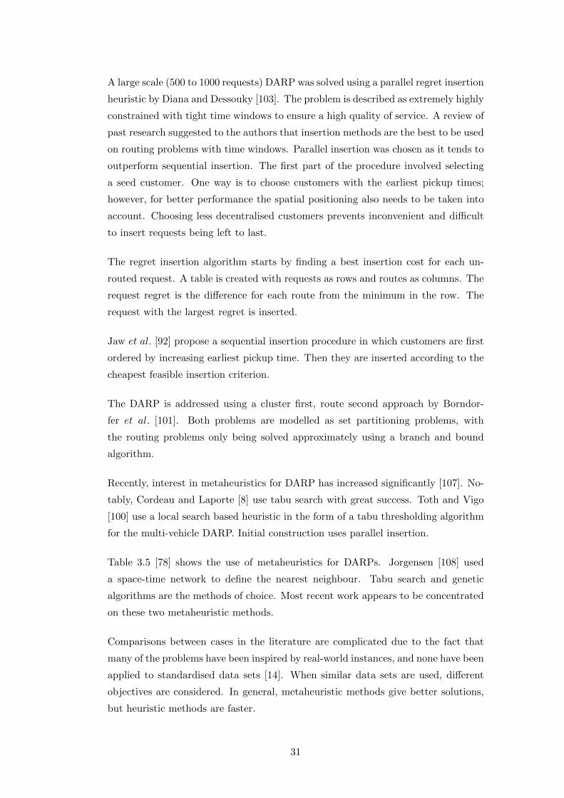
A large scale (500 to 1000 requests) DARP was solved using a parallel regret insertion
heuristic by Diana and Dessouky [103]. The problem is described as extremely highly
constrained with tight time windows to ensure a high quality of service. A review of
past research suggested to the authors that insertion methods are the best to be used
on routing problems with time windows. Parallel insertion was chosen as it tends to
outperform sequential insertion. The first part of the procedure involved selecting
a seed customer. One way is to choose customers with the earliest pickup times;
however, for better performance the spatial positioning also needs to be taken into
account. Choosing less decentralised customers prevents inconvenient and difficult
to insert requests being left to last.
The regret insertion algorithm starts by finding a best insertion cost for each un-
routed request. A table is created with requests as rows and routes as columns. The
request regret is the difference for each route from the minimum in the row. The
request with the largest regret is inserted.
Jaw et al. [92] propose a sequential insertion procedure in which customers are first
ordered by increasing earliest pickup time. Then they are inserted according to the
cheapest feasible insertion criterion.
The DARP is addressed using a cluster first, route second approach by Borndor-
fer et al. [101]. Both problems are modelled as set partitioning problems, with
the routing problems only being solved approximately using a branch and bound
algorithm.
Recently, interest in metaheuristics for DARP has increased significantly [107]. No-
tably, Cordeau and Laporte [8] use tabu search with great success. Toth and Vigo
[100] use a local search based heuristic in the form of a tabu thresholding algorithm
for the multi-vehicle DARP. Initial construction uses parallel insertion.
Table 3.5 [78] shows the use of metaheuristics for DARPs. Jorgensen [108] used
a space-time network to define the nearest neighbour. Tabu search and genetic
algorithms are the methods of choice. Most recent work appears to be concentrated
on these two metaheuristic methods.
Comparisons between cases in the literature are complicated due to the fact that
many of the problems have been inspired by real-world instances, and none have been
applied to standardised data sets [14]. When similar data sets are used, different
objectives are considered. In general, metaheuristic methods give better solutions,
but heuristic methods are faster.
31
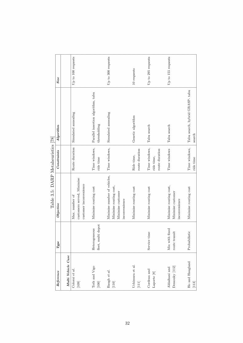
Tab
le3.
5:D
AR
PM
etah
euri
stic
s[7
8]R
efe
ren
ceT
ype
Obje
cti
ve
Con
stra
ints
Alg
ori
thm
Siz
e
Mu
lti
Vehic
leC
ase
Colo
rnietal.
Max.
nu
mb
erof
Rou
ted
ura
tion
Sim
ula
ted
an
nea
lin
gU
pto
100
requ
ests
[109]
cust
om
ers
serv
ed,
Min
imis
e
cust
om
erin
conven
ien
ce
Toth
and
Vig
oH
eter
ogen
eou
sM
inim
ise
rou
tin
gco
stT
ime
win
dow
s,P
ara
llel
inse
rtio
nalg
ori
thm
,ta
bu
[100]
flee
t,m
ult
id
epot
rid
eti
me
thre
shold
ing
Bau
ghetal.
Min
imis
enu
mb
erof
veh
icle
s,T
ime
win
dow
s,S
imu
late
dan
nea
lin
gU
pto
300
requ
ests
[110]
Min
imis
ero
uti
ng
cost
,
Min
imis
ecu
stom
er
inco
nven
ien
ce
Uch
imu
raet
al.
Min
imis
ero
uti
ng
cost
Rid
eti
me,
Gen
etic
alg
ori
thm
10
requ
ests
[111]
rou
ted
ura
tion
Cord
eau
an
dS
ervic
eti
me
Min
imis
ero
uti
ng
cost
Tim
ew
ind
ow
s,T
ab
use
arc
hU
pto
295
requ
ests
Lap
ort
e[8
]ri
de
tim
e,
rou
ted
ura
tion
Ald
aih
an
ian
dM
ixw
ith
fixed
Min
imis
ero
uti
ng
cost
,T
ime
win
dow
sT
ab
use
arc
hU
pto
155
requ
ests
Des
sou
ky
[112]
rou
tetr
an
sit
Min
imis
ecu
stom
er
inco
nven
ien
ce
Ho
an
dH
au
gla
nd
Pro
bab
ilis
tic
Min
imis
ero
uti
ng
cost
Tim
ew
ind
ow
s,T
ab
use
arc
h,
hyb
rid
GR
AS
P-
tab
u
[113]
rid
eti
me
searc
h
32
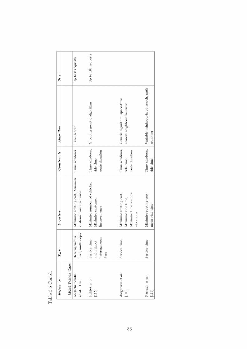
Tab
le3.5
Con
td.
Refe
ren
ceT
ype
Obje
cti
ve
Con
stra
ints
Alg
ori
thm
Siz
e
Mu
lti
Vehic
leC
ase
Mel
ach
rin
ou
dis
Het
erogen
eou
sM
inim
ise
rou
tin
gco
st,
Min
imis
eT
ime
win
dow
sT
ab
use
arc
hU
pto
8re
qu
ests
etal.
[114]
flee
t,m
ult
id
epot
cust
om
erin
conven
ien
ce
Rek
ieketal.
Ser
vic
eti
me,
Min
imis
enu
mb
erof
veh
icle
s,T
ime
win
dow
s,G
rou
pin
ggen
etic
alg
ori
thm
Up
to164
requ
ests
[115]
mu
lti
dep
ot,
Min
imis
ecu
stom
erri
de
tim
e,
het
erogen
eou
sin
conven
ien
cero
ute
du
rati
on
flee
t
Jorg
ense
netal.
Ser
vic
eti
me,
Min
imis
ero
uti
ng
cost
,T
ime
win
dow
s,G
enet
icalg
ori
thm
,sp
ace
-tim
e
[108]
Min
imis
eri
de
tim
e,ri
de
tim
e,n
eare
stn
eighb
ou
rh
euri
stic
Min
imis
eti
me
win
dow
rou
ted
ura
tion
vio
lati
on
s
Parr
aghetal.
Ser
vic
eti
me
Min
imis
ero
uti
ng
cost
,T
ime
win
dow
s,V
ari
ab
len
eighb
ou
rhood
searc
h,
path
[116]
mea
nri
de
tim
eri
de
tim
ere
lin
kin
g
33
Exact Methods There is a long history of research in exact methods for VRPs.
Due to the fact that these problems are NP -hard, complex solution methods are de-
vised, including those involving decomposition, column generation, row-generation,
or combinations thereof.
A survey of exact methods for the VRP has been done by Laporte [29]. His definition
of a VRP covers situations with a depot and customers. Exact methods can be
classified as direct tree search methods, dynamic programming or integer linear
programming (ILP).
Laporte et al. [117] [118] describe a formulation for CVRPs which exploits the
fact that an m-TSP can be transformed into a 1-TSP by introducing artificial de-
pots. The problem can be solved using a branch-and-bound process where the
sub-problems are assignment problems, as in the assignment-based solution to the
TSP (as described in [119]). Several variations of the basic VRP have been solved.
The k-degree center tree algorithm for the MCVRP was developed by Christofides
et al. [120]. They divide the edges into four subsets and devise a special formulation
accordingly.
Set partitioning has become popular in exact algorithms. In these formulations,
routes are chosen from sets of depots which make up feasible routes with a cost
minimizing objective [119]. Because the variable sets can be huge, column generation
is the natural way to address these types of problems. In such formulations, any
feasible solution is generated with only a few variables, then new routes are added
depending on the marginal cost of other possible routes. Finding these new routes
to add can, in some cases, be a challenge, and dynamic programming has been used
or shortest path [119] has been used, depending on problem features. Because of
the integer variable constraints, the procedure must be used in conjunction with a
branch-and-bound algorithm.
Three-index formulations refer to formulations where each variable xijk refers to a
specific vehicle or fleet k using an arc ij, where the variable is binary and equal to
1 if the arc is used [119]. Two-index formulations are where variables xij refer to an
arc ij only.
A number of valid inequalities (cutting planes) have been proposed for various VRPs.
One such approach is that of Cordeau [82]. Chandran and Raghavan [121] demon-
strate the use of tree structures to solve CVRPs and other VRPs. In special cases,
when a problem can be represented in tree form, a number of valid inequalities and
34
special formulations are applicable.
Exact methods for VRPPDs have been surveyed by Cordeau et al. [122]. Formula-
tions are provided for the VRPPD with time windows (VRPPDTW). Early DARP
exact formulations made use of dynamic programming (DP). Thereafter, few if any
exact formulations have been proposed, with heuristics and metaheuristics the most
commonly used techniques. According to Parragh et al. [14], the reason exact meth-
ods are not used for the DARP is that the concept of “optimal solutions” becomes
debatable for these types of problems.
3.2 Airline Scheduling
3.2.1 Scheduled Airlines
Schedule Planning and Generation
The airline schedule planning problem can be disassembled into the schedule design
problem, the fleet assignment problem, the maintenance routing problem and the
crew scheduling problem [123]. Because of the size of typical scheduled flight (or
commercial) airline companies, these problems are most often each addressed sep-
arately and often iteratively. Some work has been done on integrating some or all
of these problems. Much work has been done on solution methodologies for opti-
mising the resultant large models. Solutions are most often generated using linear
programming models of various types, including network flow and integer linear
programming (ILP). Because of the massive sizes of models, heuristics are often an
important part of the modelling and solution process. An overview of formulations
and solution methods is provided by Gronkvist [2].
Schedule Design Problem
Schedule planning involves maximizing revenues [124] by providing services to meet
expected demand. Constraints include gate facilities, available slots, connections,
etc. The schedule should be flyable with available resources. Flight legs are designed,
each leg consisting of one aircraft flight, and with an associated origin and destination
(O-D) and time of departure and time of arrival. Typically airlines must consider
peak passenger times and frequency of service, size of aircraft, competition and the
effect the provision of the services will have.
35

After generation of the schedules, fleet assignment and aircraft routing can be per-
formed.
Fleet Assignment Problem
Description This is the process of assigning the optimum aircraft type to each
leg in a schedule, to maximize revenues and minimise costs. This type of problem
is often formulated as a multi-commodity network flow problem (MCNFP) with
aircraft flowing through the network. The formulation can be done using a time-
line network (Figure 3.6), sometimes also called a time-space network, with arcs
representing flights. The different aircraft types or fleets are then the commodities.
Figure 3.6: Time-Space Network
Unfortunately such MCNF models cannot use the computationally efficient network
simplex method and must be solved using integer programming methods. Mainte-
nance considerations can be taken into account by adding constraints accordingly.
Although crew scheduling is a separate and extensive modelling effort, crew can be
taken into account in the fleet assignment phase such that more feasible and cheaper
crew schedules are likely to be available in the crew scheduling phase [2].
Kontogiorgis [125] describes using A Mathematical Programming Language (a com-
mercial mathematical modelling language, AMPL) to assign fleets for US Airways.
US Airways typically flies 2500 flights to more than a hundred markets using 400
36
aircraft of 14 different types. The model maximizes revenue and reduces costs. The
solution procedure involves solving the linear programming (LP) relaxation, fixing
variables and finally solving the reduced mixed integer program (MIP) with a branch
and bound solver to find the remaining variables. According to Rushmeier et al.
[124], such a problem could have 75000 binary variables, 1000 integer variables and
50000 constraints. Normally a solution is required within a day. The solution pro-
cess involves preprocessing, aggregating of nodes and other size reduction heuristics.
Then, based on an LP relaxation, a number of variables are fixed. After this, a
model may have 12% of the rows and 20% of the variables remaining. Subsequently
an integer solution is sought using a branch and bound method.
In some cases, fleet assignment is not necessary, for example, if the airline uses one
fleet type [126], and only aircraft routing and crew pairing is done. These are solved
iteratively to achieve a series of feasible solutions. Ray and Tomlin [127] address the
aircraft routing problem by using an IP model with time-space network and time
windows. A heuristic and LP relaxation plus rounding technique are suggested to
find good solutions.
Time-Space Networks Timespace networks have been used many times in lit-
erature to represent aircraft fleet assignment and/or routing problems and thereby
create model formulations. An example is the network used by Barnhart [3]. The
most commonly used time-space network representation is shown in Figures 3.6
and 3.7. Each node has a geographical position and time associated with it and
arcs represent movement of aircraft between nodes. Arcs can represent flight legs
or they may be “ground arcs” and represent time when an aircraft is stationary on
the ground at a specific location.
For such a model, aircraft may be grouped by fleet, such that a fleet consists of
similar, interchangeable aircraft, in which case a fleet will represent a commodity
in a multi-commodity network flow problem. The addition of passengers represents
another type of commodity, where passenger groups with different origin-destination
(O-D) pairs will each represent a different commodity. Passenger movement must
then be linked to aircraft movement using aircraft capacity constraints [128].
A “passenger leg” will typically refer to a passenger group travelling on a single, spe-
cific flight leg. Similarly, “passenger ground arcs” represent time spent by passenger
groups waiting on the ground at some location.
37
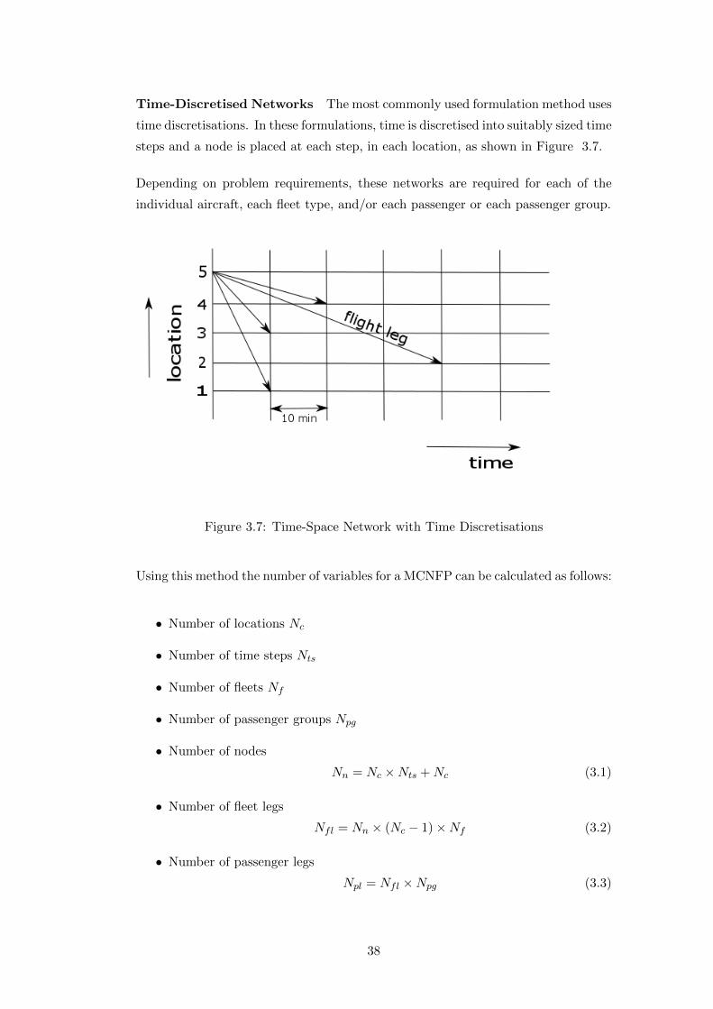
Time-Discretised Networks The most commonly used formulation method uses
time discretisations. In these formulations, time is discretised into suitably sized time
steps and a node is placed at each step, in each location, as shown in Figure 3.7.
Depending on problem requirements, these networks are required for each of the
individual aircraft, each fleet type, and/or each passenger or each passenger group.
Figure 3.7: Time-Space Network with Time Discretisations
Using this method the number of variables for a MCNFP can be calculated as follows:
• Number of locations Nc
• Number of time steps Nts
• Number of fleets Nf
• Number of passenger groups Npg
• Number of nodes
Nn = Nc ×Nts +Nc (3.1)
• Number of fleet legs
Nfl = Nn × (Nc − 1)×Nf (3.2)
• Number of passenger legs
Npl = Nfl ×Npg (3.3)
38
• Number of fleet ground arcs
Nfr = (Nn +Nc)×Nf (3.4)
• Number of passenger group ground arcs
Npr = (Nn +Nc)×Npg (3.5)
• Number of variables in problem
Nv = Nfl +Npl +Nfr +Npr (3.6)
The model time may consist of a single day, or longer periods, such as a week. For
this work, a single day is used. It should be noted that the number of fleet ground
arcs calculated (Nfr) includes ground arcs for each fleet between every node, as well
as a ground arc into the first node at every location at the start of the day, and a
ground arc out of the last node at every location at the end of the day.
With reference to Figure 3.7, the number of flight legs starting from a single node is
equal to Nc − 1 for each fleet type. The arrival time of a flight leg is the departure
node time plus the flight time. This flight time will fall between the times of two
nodes at the destination location. The later of these two nodes is assigned as the
leg arrival node.
It should be noted that flight legs that depart near the end of the day may have
arrival times which are beyond the end-of-day time, so no nodes can be assigned as
arrival nodes. These flight legs are not included in the problem. There is no way
to predict how many flight leg variables will be left out for this reason before the
problem parameters are known. The equation shown for number of fleet legs (3.2)
includes these legs and will therefore produce a higher figure than will actually be
the case for any instance.
Unfortunately in practice the size of these problems quickly grows impractically large
in terms of variables for even small-sized problems. For example, using the formulas
(3.1) to (3.6), a 7 city, 26 passenger group, 2 fleet type, 12 hour day problem with
10 minute steps will result in 177604 variables, 157248 of which are passenger group
leg variables.
In many such problems most of the variables are aircraft flight legs or passenger
legs and will never be used. The obvious solution is to use heuristics to leave out as
many unlikely-to-be-used variables as possible. These heuristics must be developed
after careful study of the specific problem.
39

Maintenance Routing Problem
The aircraft maintenance routing problem involves assigning a particular aircraft
to each flight leg [123]. Consistency with the fleet assignment problem must be
maintained. Each aircraft must be assigned a feasible sequence of flight legs such
that the periodic maintenance checks for that specific aircraft can be undertaken
within legal requirements.
Crew Scheduling Problem
This problem involves determining the cost-minimising assignments of crew to each
leg in the aircraft schedule [123]. The schedule will specify activities for a crew
member typically for a period of a month. All labour regulations must be satisfied.
The crew scheduling problem was the first of the airline scheduling sub-problems to
receive attention in 1969, see Arabeyre et al [129] for details. This was because of
the large size of such problems in practice. Typically, many possible pairings (i.e.
crew-aircraft combinations) are generated and the best combination (minimum cost)
is sought using integer programming methods [124]. Since then, many others have
considered the problem using various techniques.
Integrated Models
Integrated scheduling refers to combining routing, scheduling, fleet assignment and
crew scheduling [130]. This has been addressed by Barnhart [131] using flight strings.
Papadakos [130] presents an integrated model including fleet assignment, aircraft
maintenance routing and crew scheduling. The problem is solved using enhanced
Benders decomposition and accelerated column generation.
A warm-start type of model was developed by Stojkovic et al [132]. The model re-
optimizes a schedule after a perturbation (disruption), and therefore must be able
to generate real-time data. This problem is often referred to as the day-of-operation
changes model [133]. The problem was a linear programming problem, and the dual
of the problem was a network problem and therefore relatively easily solvable using
the network simplex method.
An integrated scheduling method is devised by Haouari et al. [134]. They use
a 2-phase network flow heuristic which starts with clustering flights and assigning
40

aircraft to flights using a greedy heuristic. Thereafter a series of assignment problems
are solved, and a further set of MCNF problems solved in phase 2.
3.2.2 Charter Airlines
Charter airline scheduling has been addressed by a number of researchers. This
work has been mostly restricted to the case where demand need not be completely
satisfied. Erdman et al. [133] have proposed a schedule generation problem for a
charter airline to maximize profits. The model is a capacitated network model with
side constraints (i.e. an ILP). Variables relate to aircraft rotations (daily routes
or itineraries). Since the model provides weak relaxations, cutting plane methods
of relaxation tightening are proposed. Essentially, the constraint causing the weak
relaxations was identified as the constraint restricting the number of passengers
transported due to the aircraft capacity. This was addressed by adding suitable
cutting plane constraints to limit passenger demand to aircraft size.
Kim and Barnhart [135] consider the charter airline service network design problem
by developing exact and heuristic network design models. They develop a fast
method for a single fleet model and adapt it to create a heuristic approach to the
multiple fleet model. Weak relaxations were improved by adding constraints forcing
at least one aircraft to be assigned to a group of passengers. For large instances, a
column generation scheme is proposed where aircraft itineraries with reduced costs
are sought by means of shortest path type sub-problems.
Yan and Tseng [128] developed a demand-driven integrated fleet routing and flight
scheduling model for a charter airline company, i.e., where not all demand needed to
be met. They use a fleet flow time-space network for each fleet type, as well as a pas-
senger flow time-space network for each demand (O-D) pair. Time discretisations are
used. The model is a cost minimising multi-commodity network flow problem. The
resulting large-sized problem is solved using Lagrangian relaxation, a sub-gradient
method, specialised heuristics and a custom-designed solution sequence. The model
was applied to a Taiwanese airline with 11 cities served by 170 daily flights and 2
fleet types. The model had 9504 nodes, 25558 arcs and 10407 constraints.
3.2.3 On-Demand Air Transportation
In 2004, Cordeau et al. [5] compiled a literature review on the transportation on
demand (TOD) types of problems. They found little or no literature for the static
41
dial-a-flight problem (DAFP) and therefore presented an ILP formulation. The
static version must schedule a known number of demands in a day. The dynamic
version of the DAFP addresses the problem where passengers may arrive and re-
quest service immediately, but then may be denied service at some cost to the
provider. The suggested time-discretised multi-commodity network flow problem
becomes large quickly, and specialised methods are required to solve instances in-
volving 15 to 30 airports and 5 to 10 airplanes. It should be noted that the problem
at hand matches this type of problem. Therefore, the problem descriptions “DAFP”
and “airline taxi” are used interchangeably in this work.
Courier services operate a type of on-demand delivery service. Armacost et al. [136]
describes a system developed to schedule packages for United Parcel Service (UPS),
an American courier company. UPS delivers 13 million packages globally every
day. The model determines aircraft routes, fleet assignments and package routings.
The main problem with the formulation used, as with many such problems, was
the weakness of relaxations. A solution involved redefining the decision variables
as composite variables. Effectively, instead of using the actual aircraft decision
variables, new variables specifically designed to have sufficient capacity to carry the
full parcel loads that are needed to be transported are defined. For example, if one
aircraft type is too small to carry the load, another decision variable is introduced
which represents two of that aircraft type in one variable.
Business and service considerations for the DAFP include how many stops a pas-
senger may experience, passengers changing planes at stops, waiting times and total
journey times (Cordeau et al. [5]). In terms of costs, short flights use more fuel per
km of distance flown than long flights. Fuel consumption is also dependent on how
heavily loaded the aircraft is.
The turnaround time refers to the time it takes for an aircraft to be ready to take
off after having landed and stopped to offload and take on new passengers. There
are varying amounts of turnaround time necessary, depending on factors such as
whether passengers and their baggage must change aircraft, number of passengers
in the aircraft, whether refueling is required and aircraft size.
An on-demand air transportation type of problem was addressed by Ronen [137]. A
set of revenue trips needed to be partially satisfied by a fleet of aircraft at minimal
cost, and any remaining flights were to be sold to other operators. A large set of
feasible candidate schedules is generated for each aircraft using heuristics. The best
set is then selected using an MIP-type solver.
42
Lee et al. [6] address the air taxi service problem with probabilistic variables. They
model the situation where passengers must request the service in advance, as opposed
to simply arriving when transport is needed. Discrete event simulation methods to
maximize revenues are used.
The most recent literature dealing with the airline taxi problem is that of Espinoza
et al [7]. The research dealt with the hiring of executive jets in the USA and is
termed the per-seat, on-demand air transportation problem (PSOD). This problem
description closely matches that of the problem at hand, suggesting the PSOD is
similar to the airline taxi problem to be addressed.
In such a problem, business people provide a required origin-destination (O-D) pair
(demand) and timing window a few days or one day in advance, and the jet provider
must assemble a schedule to accommodate all of these bookings. A time-discretised
network model resulted in a multi-commodity network flow model with side con-
straints. Heuristics designed to eliminate obviously infeasible routes are captured
in the form of a rolling forward algorithm. These heuristics relate to plane capac-
ity, timing constraints such as time of day, elimination of sequences which involve
two consecutive flights without passengers on board, eliminating later departures in
flight sequences if earlier departures are available. Time windows are also intelli-
gently chosen such as to coincide with key moments of the day, hopefully eliminating
the need for many variables. Aggregation of nodes was carried out to further re-
duce the network size. This involved eliminating arcs and nodes. Problems of up to
81 requests, 8 jets and 17 airports are solved. A second paper [138] describes im-
proved neighbourhood search techniques and parallelisation of the search to achieve
solutions for larger instances.
The on-demand air transportation problem or DAFP or airline taxi problem is to
some extent similar to certain vehicle routing problems such as PDPs, since both
have pickups and deliveries and time windows. It differs from the DARP in that, in
an airline taxi scheduling problem, all passengers must be picked up and dropped
off at predefined points, namely airports, whereas in the DARP, passengers can be
picked up and dropped off anywhere on the network.
This means there are likely to be fewer locations in a DAFP than a DARP for
a similar number of bookings, allowing a smaller-sized formulation for the DAFP.
Different heuristics might be applicable. In practice in a DAFP, it is often acceptable
from a quality of service point of view to drop off passengers at a location such
that they can be collected by another vehicle to continue their journey. This is
not only unlikely to be acceptable in a DARP, but, due to the random positioning
43

of each passenger pickup and delivery points, there should be fewer cost-effective
opportunities to do this.
3.3 Solving large MIP problems
Aircraft scheduling problems often have large numbers of variables, including many
binary variables. Integer and continuous variables may also be present. Such prob-
lems can be easier to solve by, for example, reducing variable count at the expense
of more constraints, or by exploiting special structures related to the binary vari-
ables [139] . More constraints help with respect to integer solution methods by
reducing the size of the search space, but can slow down the solution of the linear
programming (LP) relaxations.
In practice, various mathematical solution algorithms and methods are used, includ-
ing decomposition, column generation, branch, price and cut. The objective function
can be modified by means of Lagrangian multipliers to effectively remove difficult
constraints and result in a problem with a simple structure. This might be done,
for example, to allow the model to be solved using an efficient network algorithm
[2]. Typically, the aircraft capacity constraints are dealt with in this manner.
Column generation is a well-established technique which involves progressively adding
variables to the problem and proceeding with LP relaxation solutions accordingly
[140]. The technique applied to IP is referred to by the term ‘branch and price’.
Branch and price has become popular for many VRP problems. Examples include
those of Salani, Fukasawa et al. and Prescott-Gagnon et al. [141–143]. There are
issues which arise and make these methods more suited to achieving good solutions
than optimal solutions. For example, the method normally involves a reformulation
of the problem such that variables inherently contain more information. This allows
each variable to be priced to determine if it should be in a solution or not. The prob-
lem then revolves around how to make up or select feasible integer variables that
should be included in the problem. This search procedure is done at each branch of
the branch and bound process, and is sometimes done using dynamic programming
(DP) or metaheuristics. The technique has been successfully applied to a number
of routing-type problems.
Branch and cut involves leaving constraints out of the LP relaxation. Then, if a
solution is infeasible, a subproblem (the separation problem) is solved to identify
violated inequalities. Some of these are added to the LP to cut the infeasible region
44
off. Branching occurs when no violated inequalities are found. Both techniques can
be used on a problem simultaneously.
Feaspump [22] is a heuristic method which works by considering two solutions, the
feasible LP relaxation optimum and an integer solution which is the LP rounded
solution and thus may or may not be optimum. The idea is to search in the di-
rection of the LP optimum for a better integer solution. This is done by finding
the closest LP feasible point to the current infeasible integer solution. The method
first addresses the binary variables, then having fixed them, attends to the general
integer variables.
Benders [23] proposed what is now called Bender’s decomposition. Effectively, the
MIP problem is decomposed by variable type. This or modifications thereof may
have advantages in practice since efficient methods can often be developed to solve
problems with purely one kind of variable, but not mixed types. Papadakos [130]
uses Benders decomposition in this way in a necessarily large integrated model for
airline scheduling.
Kamath et al. [144] and Karger and Plotkin [145] have developed fast approxima-
tion algorithms for the minimum cost multi-commodity network flow problem. The
algorithm starts with zero flow and at each iteration, identifies incremental flows in
the network.
45
3.4 Conclusions from Literature Review
There has been a substantial amount of work done on heuristics for VRP problems in
general. In recent heuristic research, construction heuristics such as greedy heuris-
tics, insertion heuristics and clustering, including cluster-first route-second methods,
are favoured.
The latest dial-a-ride problem research is dominated by tabu search and genetic
algorithm based methods. A wide range of sizes of problems have been approached
with these methods. Exact methods tend to be avoided for multi-vehicle pickup and
delivery problems in particular.
Work on agent routing, including ACO, for VRPs is becoming more popular. Apart
from ACO and other nature-based methods, there seems to be little, if any, work on
training of agents in agent-based routing.
There is very little work on the airline taxi problem in published literature.
46
4 Methodology
4.1 Overview
The type and size of the problem at hand suggests it could be approached by ap-
plying similar techniques as have been used for the DARP, such as the use of im-
provement heuristics or local search-based metaheuristics. Compared to the large
DARP described by Diana and Dessouky [103], this problem is relatively small and
less tightly constrained, since many of the customers have wide time window re-
quirements. However, it would be regarded as fairly tightly constrained compared
to many VRPTW research problems, such as the VRPTWs used by Solomon [25].
In general, heuristic methods give lower quality solutions than metaheuristic meth-
ods [5]. The nature of the problem suggests solution methods for reasonably tightly
constrained and medium-sized problems, such as exact or metaheuristic methods.
Very little work has been done on construction methods which is the focus of this
research. Theoretically, if good solutions can be obtained in a reasonable time using
a construction method, improvement heuristics might not be needed, or need less
time to improve the solution.
A reason to avoid the use of purely heuristic methods is the cost of the service. Since
the service is provided by an expensive vehicle type, the cost of a less than optimal
solution is high compared to a road-based taxi service.
In this work, a pure version of the airline taxi problem was addressed using the
relevant Sefofane Air data, but leaving out certain constraints. A small problem
was created to test the methods and for benchmarking purposes. Thereafter, the
problem with all constraints was addressed.
47
Constraints that were relaxed included:
• No forced end-of-day positions for aircraft for certain versions of the problem.
• No special considerations with regard to the number of crew required or spe-
cial customer requests (customers can request special arrangements for their
journey).
For PDPs, particularly real-world problems, it is considered difficult to construct
feasible solutions [15]. However, existing literature is concentrated around improve-
ment heuristics and metaheuristic techniques, which need such a feasible solution
to begin. Metaheuristic techniques are beneficial because the actual, constrained
feasible region in these problems can be small. Therefore methods to produce good
starting feasible solutions for such problems are required.
The full problem, as experienced by Sefofane Air, is first described in detail in
Chapter 5. Thereafter various approaches to the solution of the air taxi problem
that underlies it are detailed.
The problem described in this work can be addressed using an exact ILP and prob-
lem size reduction heuristics, as done by Espinoza et al. [7]. Such an exact method
is presented in Chapter 6, together with newly-developed heuristics in Chapter 7.
This method involves the use of a multi commodity network flow (MCNF) integer
linear program (ILP) with time discretisations (TDs). This method was initially
devised purely to obtain benchmark solutions as close to optimality as possible.
However, when combined with heuristics devised for this problem, it will be a prac-
tical alternative for smaller instances, possibly up to 80 requests. Two heuristics are
developed in Chapter 7 for this problem. They are designed to reduce the number
of variables in the problem by aggregation of customer groups and by eliminating
cost-ineffective routes.
Another approach to the problem is to combine exact ILP methods with construc-
tion heuristics, by using heuristics to construct feasible route sections and use those
as variables in ILP formulations (as done by Ronen [137] and Armacost et al. [136]).
This way, more information is captured in each variable than a typical exact formu-
lation, and fewer variables will result. It is these ideas which motivate the following
methods which are proposed in this research:
1. MCNFP with time discretisations (TDs): Chapters 6 and 7 - A group
aggregation heuristic and a geographically-inspired heuristic are designed to
48
reduce the number of variables associated with the passenger group networks
in the standard MCNFP of Chapter 6. Although this method was initally
included to obtain a lower bound for the problem, it will be useful for smaller
problem instances.
2. Variable construction using agent routing information combined with
MCNFP : Chapter 8 - This method is similar to that described in method
1, except it only uses well-placed nodes and arcs in the networks. This infor-
mation is provided by the use of agents.
3. Composite variable MCNFP: Chapter 9 - This method creates variables
where each variable inherently contains more information than the variables in
methods 1 and 2. Specifically, the variables are created such that no passenger
networks are required, greatly reducing the size of the problem, particularly
for the problem described here.
In order to evaluate whether these methods may be useful in other VRPs, the
composite variable MCNF method (method 3) was applied to an additional VRP,
namely the MVCVRP. The agent route variable generation method (method 2) was
applied to the CVRPTW.
All models except those in Chapter 5 were generated and solved on a Mecer PC with
Intel i7 8 core processor, 8 GB RAM, Windows 7, and with Matlab 7.11, Excel 2010
and CPLEX 12.1 software packages. Chapter 5 models were solved using GUROBI
solver provided by NEOS [146].
4.2 Small-Scale Benchmark Airline Taxi Problem
For the pure airline taxi problem, a small problem was compiled in addition to the
given, relaxed and full-sized problem, such that various techniques could be tested
and for benchmark comparison purposes. The problem was formulated from the real
data such that it was suitable in terms of size and solution speed for the evaluation
of the heuristics and for comparing results from different models. It also had to
be representative geographically of the spread of landing strips (or locations) in the
full-size (large) problem.
In order to ensure the small problem was representative of real data which may
actually occur, the problem was compiled by using Monte Carlo random sampling
from the full table of 158 bookings. In doing this, the locations which appear
49
in the smaller problem should be nearly as scattered and widespread as in the
larger problem. If this is not the case, the heuristics devised may not work in the
same manner on both problems, particularly if those heuristics are related to the
geography of the locations.
The first seven locations in the full city list (see Figure 5.3 and Appendix A, Table
A.4) were chosen to be included in the smaller schedule, since they included the
hub at Maun and satisfied the requirements with regard to geographic spread. A
sampling table was assembled consisting of all bookings from the full list which only
included these seven locations.
Individual bookings were randomly sampled using a uniform distribution with re-
placement from this sampling table. Replacement is done to ensure samples are
independent. In this case, many samples are in any case similar and obtaining more
than one of the same sample does not affect the obtained sample or the solution
process in an adverse manner. The sampling process continued until 40 bookings
had been compiled.
4.3 Sefofane Air Solution
One of the solutions obtained for the full-sized model was used to demonstrate how
Sefofane Air would use this solution method in practice. The solution is compared
with the actual solution used on the day in question.
4.4 Application to Other VRPs
The composite variable MCNF method was applied to a real-world MVCVRP to
evaluate whether it may be useful for different types of VRP problems. The MVCVRP
was inspired by a real-life logistics problem for a food distributor in Pretoria, South
Africa, and as such the problem specifications match the operations of the company
in question. Two reduced-size problems were created, a small and medium size
version, in order to compare solutions with their exact solution counterparts found
using a standard ILP. A large-size problem instance provided by the company was
solved. Problems addressed represented a range of customer daily deliveries from
10 to 128 from a single depot. The presence of a single depot means that this type
of problem differs significantly from the PDP-type problems and the airline taxi
problem.
50
Another type of problem which shares commonality in terms of having a single depot
with the MVCVRP is the VRPTW. Standard, benchmark instances for this type
of problem have been artificially generated and are available on the Internet, and
such a problem, provided by Solomon [147], was obtained. For this problem, the
agent routing method developed for the airline taxi problem was applied. To achieve
this, the problem is modelled using a time-space network. A best known solution
available on the Internet was used for comparison purposes.
51

5 The Sefofane Air Scheduling Problem
Description
5.1 Sefofane Air Operations
Sefofane Air is the largest airline operating in the Okavango Swamps, Botswana,
and that is where the bulk of their operations occur. Their primary target market is
tourist groups. Their operations also include airline services in Namibia, Zimbabwe,
Zambia and South Africa.
Tourists book to stay at any of more than 100 tourist safari camps in the Okavango
and surrounding area. When booking, they will also book flights between locations
in the area.
Tourists may enter Botswana by road or on flights from South Africa or other in-
ternational locations. Typically a road trip or an international flight will bring
tourists to Victoria Falls in Zimbabwe, Livingstone in Zambia or, most likely, Maun
in Botswana, which is also where the Sefofane Air head office is located. This can be
considered the hub of their operations, since more of their flights arrive and depart
from there than anywhere else. Air Botswana international flights land and depart
from Maun.
From Maun or other point of access, Sefofane Air transports the tourist groups to
their prebooked safari camps. Most safari camps have an airstrip, and most are
an untarred (dust) landing strip. Main centres such as Victoria Falls have tarred
landing strips or airports. Often, tourists will stay in a series of different safari
camps, in which case Sefofane Air will transport them between these camps, as
required.
Sefofane Air uses relatively small aircraft designed to operate to and from such
locations. These include the Cessna C206, a 5-seater aircraft (i.e. 5 passenger seats)
52

often described as the “workhorse of the bush” (Figure 5.1), and the Cessna C208
Grand Caravan, a larger, 12-seater aircraft (Figure 5.2). Both aircraft can be flown
by a single pilot. However, if carrying passengers and luggage, the C208 needs a
loadmaster, which is an extra crew member required to balance the aircraft load
before takeoff, particularly if the aircraft is full or heavily loaded.
Figure 5.1: Cessna C206 [148]
Currently, Sefofane Air employs two experienced schedulers who make up the flight
schedule and route the aircraft a few days in advance of the day in question. The
schedulers are considered to produce good, low cost schedules. However, since the
job they do is dependent on their experience, there is a risk to the airline that, if
they should not be available, at best schedule costs would increase, and at worst the
airline would not be able to operate effectively.
Because schedules are assembled in advance for a known booking list, the problem
can be classified as a static DAFP [122].
5.2 Problem Specifications
Sefofane Air’s fleet and aircraft specifications, as used in the Okavango Swamps, are
shown in Table 5.1.
53
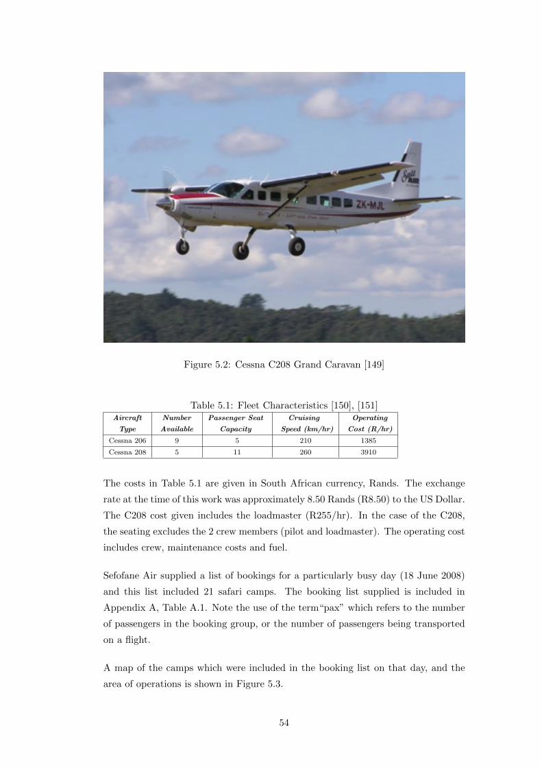
Figure 5.2: Cessna C208 Grand Caravan [149]
Table 5.1: Fleet Characteristics [150], [151]Aircraft Number Passenger Seat Cruising Operating
Type Available Capacity Speed (km/hr) Cost (R/hr)
Cessna 206 9 5 210 1385
Cessna 208 5 11 260 3910
The costs in Table 5.1 are given in South African currency, Rands. The exchange
rate at the time of this work was approximately 8.50 Rands (R8.50) to the US Dollar.
The C208 cost given includes the loadmaster (R255/hr). In the case of the C208,
the seating excludes the 2 crew members (pilot and loadmaster). The operating cost
includes crew, maintenance costs and fuel.
Sefofane Air supplied a list of bookings for a particularly busy day (18 June 2008)
and this list included 21 safari camps. The booking list supplied is included in
Appendix A, Table A.1. Note the use of the term“pax” which refers to the number
of passengers in the booking group, or the number of passengers being transported
on a flight.
A map of the camps which were included in the booking list on that day, and the
area of operations is shown in Figure 5.3.
54
In this research, each safari camp (or location) was arbitrarily assigned a number
from 1 to 21 for the purposes of modelling, and these numbers are shown on the
map. The safari camp names and numbers are listed in Appendix A, Table A.4.
The distances between safari camps is included in Appendix A, Table A.2.
55
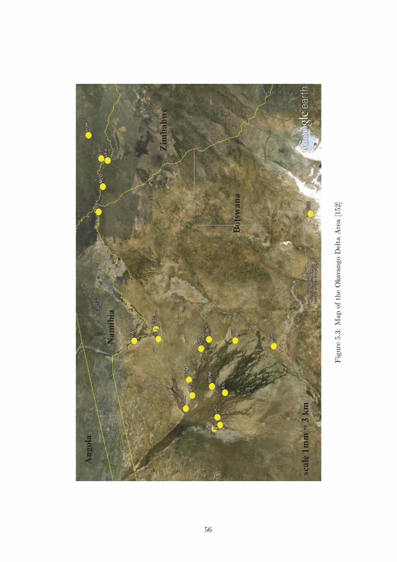
Fig
ure
5.3:
Map
ofth
eO
kava
ngo
Del
taA
rea
[152]
56
Sefofane Air supplied the manual schedule that was compiled and actually used for
the day in question, and this is included in Appendix B. This schedule shows that
the schedulers use a turnaround time of 10 minutes.
Sefofane Air have 3 different types of passengers:
1. Tourists - Usually travelling in groups of mostly 2 but also more.
2. Sefofane and safari camp staff - Usually travelling as a single person.
3. Boxes - A box consists of provisions for the camps and takes up one seat on
an aircraft.
It is desirable not to have tourists sitting next to boxes, hence in the schedule shown,
the boxes were grouped either in 5s or in 12s such that they would alone take up
their own aircraft.
For the C208, no loadmaster is required for “box only” flights. Examination of the
manual schedule (Appendix B) reveals an instance where a C208 had no loadmaster,
and had to fly to a certain destination to collect one. Also, all the “box only” trips
were specifically scheduled without a load master. Presumably this saves costs and
allows one extra box to be transported.
Crew may overnight at any safari camp, since the aircraft is merely parked on the
airstrip and the crew accommodated in available accommodation. However, it may
be advantageous to ensure they are at some specific destination, for example, to start
the next day’s flights. In fact, examining the manual schedule, it is apparent that
the schedulers did schedule aircraft to fly empty to overnight at specific destinations.
Note that both aircraft have relatively long ranges so refueling during a day’s flying
is unlikely to be necessary, and this was actually the case in this work. If necessary,
fuel is available at the main hub (Maun) and various other stops such as Victoria
Falls and Livingstone.
Pilots and loadmasters are paid per hour of flying time. The loadmaster’s cost is
relatively small compared to the C208 operation cost (R255 vs R3610). This, coupled
with the fact that the flights requiring a loadmaster far outnumber the flights which
do not, suggest the airline should consider always including a loadmaster in every
flight. This is because the operational complications of not having a loadmaster on
certain flights is likely to outweigh the small cost benefit.
Examination of the manual schedule revealed a special request. This involved a
57

large tourist group which wanted to be flown in their own aircraft and without any
other passengers. Since the group consisted of 13 people, they requested two C208s
for this purpose.
58
6 Multi-Commodity Network Flow ILP with
Time Discretisations
6.1 Description
As suggested by Cordeau [5], Yan and Tseng [128] and Espinoza [7], the DAFP can
be formulated as an ILP with the use of time steps or discretisations (TDs). In this
case, the time-space diagram is discretised in the time dimension using 10 minute
time steps. A node is placed at each destination at each time step, and all possible
flight arcs are included, as shown in Figure 3.7. Nodes are also placed at each
passenger origin at the earliest departure time (EDT) and destination at the latest
arrival time (LAT). These nodes are used to ensure ground arcs can be included that
will allow demand to be met as required by the time windows. Multiple networks
are superimposed and solved in the formulation, one network for each fleet type and
one for each passenger group.
The formulation is as follows:
Define the following decision variables:
• Set of aircraft flight variables X, consisting of elements xijf , each correspond-
ing to a possible flight leg. Each such leg is associated with a fleet type f in
the set of fleet types F , a starting node iut in the set of nodes N with an origin
u from the set of locations C, and a departure time t, and an ending node jvt
in the set of nodes N with a destination v ∈ C and an arrival time t. These
variables are referred to as “flight legs” and are integer.
• Set of fleet ground variables S, consisting of elements sijf , each corresponding
to a fleet type f in the set of fleet types F , a start node iut and end node
jut, both in set of nodes N . A ground variable has an associated location u
59
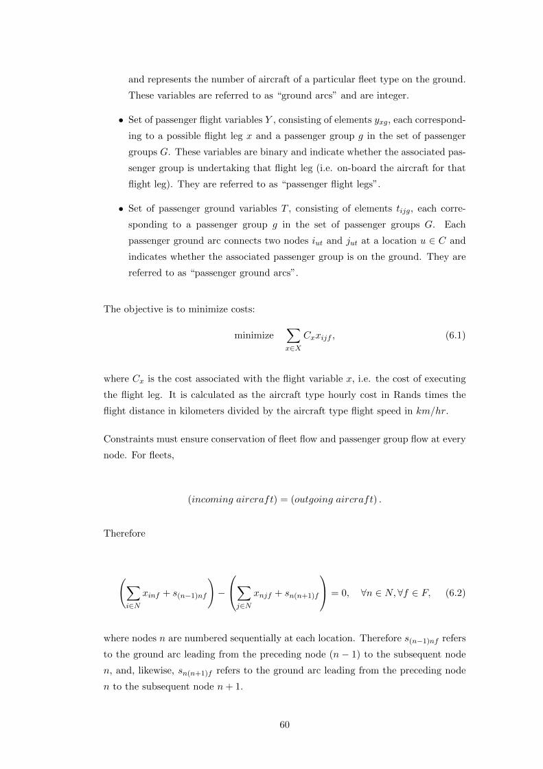
and represents the number of aircraft of a particular fleet type on the ground.
These variables are referred to as “ground arcs” and are integer.
• Set of passenger flight variables Y , consisting of elements yxg, each correspond-
ing to a possible flight leg x and a passenger group g in the set of passenger
groups G. These variables are binary and indicate whether the associated pas-
senger group is undertaking that flight leg (i.e. on-board the aircraft for that
flight leg). They are referred to as “passenger flight legs”.
• Set of passenger ground variables T , consisting of elements tijg, each corre-
sponding to a passenger group g in the set of passenger groups G. Each
passenger ground arc connects two nodes iut and jut at a location u ∈ C and
indicates whether the associated passenger group is on the ground. They are
referred to as “passenger ground arcs”.
The objective is to minimize costs:
minimize∑x∈X
Cxxijf , (6.1)
where Cx is the cost associated with the flight variable x, i.e. the cost of executing
the flight leg. It is calculated as the aircraft type hourly cost in Rands times the
flight distance in kilometers divided by the aircraft type flight speed in km/hr.
Constraints must ensure conservation of fleet flow and passenger group flow at every
node. For fleets,
(incoming aircraft) = (outgoing aircraft) .
Therefore
(∑i∈N
xinf + s(n−1)nf
)−
∑j∈N
xnjf + sn(n+1)f
= 0, ∀n ∈ N, ∀f ∈ F, (6.2)
where nodes n are numbered sequentially at each location. Therefore s(n−1)nf refers
to the ground arc leading from the preceding node (n − 1) to the subsequent node
n, and, likewise, sn(n+1)f refers to the ground arc leading from the preceding node
n to the subsequent node n+ 1.
60
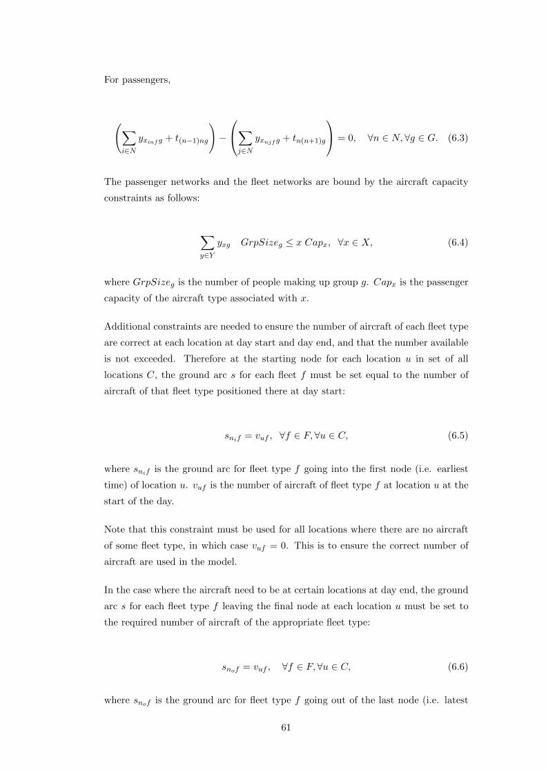
For passengers,
(∑i∈N
yxinfg + t(n−1)ng
)−
∑j∈N
yxnjfg + tn(n+1)g
= 0, ∀n ∈ N, ∀g ∈ G. (6.3)
The passenger networks and the fleet networks are bound by the aircraft capacity
constraints as follows:
∑y∈Y
yxg GrpSizeg ≤ x Capx, ∀x ∈ X, (6.4)
where GrpSizeg is the number of people making up group g. Capx is the passenger
capacity of the aircraft type associated with x.
Additional constraints are needed to ensure the number of aircraft of each fleet type
are correct at each location at day start and day end, and that the number available
is not exceeded. Therefore at the starting node for each location u in set of all
locations C, the ground arc s for each fleet f must be set equal to the number of
aircraft of that fleet type positioned there at day start:
snif = vuf , ∀f ∈ F,∀u ∈ C, (6.5)
where snif is the ground arc for fleet type f going into the first node (i.e. earliest
time) of location u. vuf is the number of aircraft of fleet type f at location u at the
start of the day.
Note that this constraint must be used for all locations where there are no aircraft
of some fleet type, in which case vuf = 0. This is to ensure the correct number of
aircraft are used in the model.
In the case where the aircraft need to be at certain locations at day end, the ground
arc s for each fleet type f leaving the final node at each location u must be set to
the required number of aircraft of the appropriate fleet type:
snof = vuf , ∀f ∈ F,∀u ∈ C, (6.6)
where snof is the ground arc for fleet type f going out of the last node (i.e. latest
61

time) of location u. vuf is the number of aircraft of fleet type f at location u at the
end of the day. This constraint could be used only for locations where aircraft are
required at the end of the day if necessary, and not all locations.
A similar constraint is required to ensure the correct number of each passenger
group in the problem. This can be done by setting the passenger ground arc into
the earliest node at each location (i.e. at day start) to either one if that location
matches the group origin, or zero otherwise. This is achieved as follows:
tnig = bug, ∀g ∈ G, ∀u ∈ C, (6.7)
where tnig is the passenger group ground arc with end node corresponding to the
first node at location u and bug is either 1 or zero, depending on whether u is the
origin for g.
Constraints must be included to ensure passenger groups are at the correct locations
at the group EDT and LAT of each day to ensure that demand is met and time
windows enforced. For the EDT, the passenger ground arcs t for every passenger
group g into the correct node of each location u must be set to a value of 1:
tneg = 1, ∀g ∈ G, (6.8)
where tneg is the passenger group ground arc with end node corresponding to EDT
and origin location for passenger group g.
Similarly, the passenger ground arcs out of the LAT nodes at each location must be
set to 1 for each passenger group:
tnlg = 1, ∀g ∈ G, (6.9)
where tnlg is the passenger group ground arc with start node corresponding to LAT
and destination location for passenger group g.
Note that this formulation allows passenger groups to swap aircraft during multi-leg
journeys. Preventing this effect would require additional variables to be introduced
into the problem, adding complexity and slowing computational times. In practice,
it was found that in addition to aircraft swapping by passenger groups, certain
passenger groups also had to endure long waiting times during journeys. A constraint
62

was introduced to constrain this intra-journey waiting time. This constraint was
formulated to limit the amount of ground arc time endured when the group was not
at either their origin or their destination, as follows:
∑t∈{T :gcod}
t ≤ 4, ∀g ∈ G. (6.10)
In equation (6.10), set {T : gcod} is a subset of passenger ground arcs T which includes
only ground arcs which are not situated at either the passenger group g origin or
destination. This will cause every group to only need to endure ground waiting times
of a maximum of 10 minutes at each stop, plus 4 x 10 = 40 minutes, i.e. 50 minutes
(10 minutes being the size of the time discretisations, TDs). Replacing the 4 by a
0 causes the passenger groups to only have ground waiting times of 10 minutes per
stop during a journey.
In practice it was found that passenger leg and ground arc variables were being
used unnecessarily since they do not have a cost associated with them. Therefore
a nominal cost was applied to all the variables except the flight leg variables to
prevent them being used in a solution. A value of 20 was found to be sufficient for
this purpose.
The number of variables produced by this formulation for the full-sized problem
under consideration in this work was found to be 7.8 million. This is too many to
create and manipulate on a personal computer. Therefore, problem size reduction
heuristics are described in the next chapter.
63
7 Heuristics for Problem Size Reduction
7.1 Motivation
The exact formulation MCNFP ILP with time discretisations (TDs) is difficult to
solve largely because of the number of passenger groups in the problem. This is
because each commodity in the problem requires a separate network, and each pas-
senger group and each fleet effectively represents a different commodity. Since for
this problem there are 2 fleet types and 158 passenger groups, the formulation results
in 7.8 million variables, which is too many to allow a solution to be obtained. The
main problem is the number of passenger groups. Therefore, heuristics are aimed
specifically at reducing:
1. The size of the passenger networks,
2. The number of passenger networks required.
In this work, two heuristics were devised to reduce the number of passenger network
variables. The first, a passenger group aggregation heuristic, effectively reduced the
number of passenger groups in the problem by half. Thus the number of passenger
networks required was reduced proportionately. The second, a heuristic based on
geographic considerations, reduced the passenger network sizes, such that, in the
large instance (full schedule) the remaining problem variables were reduced to a half
of their original number. These two heuristics were used together for the standard
MCNF described in Chapter 6 and also for the method described in Chapter 8. Only
the passenger aggregation heuristic was used in the method described in Chapter 9.
64
7.2 Group Aggregation Heuristic
7.2.1 Description
Since many bookings involve only one person (staff), the number of items to be
scheduled could effectively be reduced using a heuristic to combine smaller groups
into larger groups. For this problem, this was the case. This heuristic was devised
as follows:
1. Begin with the first booking in the list.
2. Search from the second booking onwards for any other booking which satisfies
the following:
• Has the same origin and destination as the first booking
• Has an earliest departure time (start of time window, EDT) and latest
arrival time (end of time window, LAT) closely matching that of the first
booking
• When the number of passengers in the booking is added to that of the
first booking, the aircraft capacity for the largest aircraft (C208) is not
exceeded.
3. If found, that booking is combined with the first booking and the EDT and
LAT for the combined booking is set to the later of the two in the case of
EDT, and the earlier in the case of the LAT.
4. If the plane (the largest) has additional space available, the search is continued
to the end of the booking list.
5. Move to the next booking in the list and return to step 2. Repeat until every
item in the booking list has been considered for combination with every other
item.
Note that item 2 specifies that two groups can be aggregated if their EDTs and LATs
closely match. The time within which two group times could be considered “close”
can be varied. A larger tolerance would cause more groups to be aggregated and
a smaller resultant aggregated schedule. The value used in this work is 15 minutes
and was found to produce good results.
Note that groups were simply assembled into as large groups as possible to fit in the
largest available aircraft (i.e. maximum group size of 11).
65
7.2.2 Aggregation Validation
This heuristic was validated by randomly shuffling the full set of booking data, then
observing whether different aggregated groups resulted when the heuristic was ap-
plied. The data was thus shuffled and the heuristic applied five times, and the result
was identical each time, that is, the same groups were aggregated together and the
same number of combined groups resulted. It was concluded that, in this instance,
the grouping mechanism would always produce repeatable resultant bookings.
The result for the large schedule (158 bookings/passenger groups, 21 locations) was
79 combined groups. These groups consisted of 3 combined groups that had been
assembled from 11 of the original groups, 1 combined group from 10 original groups,
1 combined group from 6 original groups, 1 combined group from 5 original groups, 2
combined groups from 4 original groups, 5 combined groups from 3 original groups,
and 15 combined groups from 2 original groups. The balance of the groups could
not be combined. The aggregated groups are shown in Appendix C. The effective
number of bookings was reduced by half for the full-sized schedule. The application
of this heuristic to the small-sized problem (40 bookings, 7 locations) resulted in 26
aggregated passenger groups.
It should be noted that, although this heuristic was effective in this instance, some
problem parameters could differ in other instances and cause the heuristic to be less
effective. For example, for this work the largest aircraft size was 11 passengers in
comparison with 5 passengers for the smaller aircraft type. There were 5 of the
larger aircraft type available. In a similar case, but where there is only one of the
larger aircraft available, the problem may become infeasible due to this heuristic, or
give much lower quality results. This is because there could be too many aggregated
groups larger than the smaller aircraft capacity of 5 passengers for the single larger
aircraft to transport in a day. In such a case, the heuristic would be executed to
only allow a limited number of large groups for the large aircraft, and the rest of
the groups of sizes up to a maximum of the size of the smaller aircraft.
7.3 Geographic Heuristic
7.3.1 Description
A heuristic based on geographical considerations was devised which limited the
generation of passenger legs in the MCNFP formulations. The heuristic is based
66
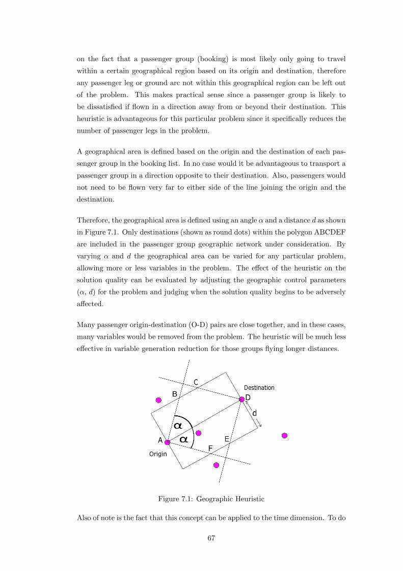
on the fact that a passenger group (booking) is most likely only going to travel
within a certain geographical region based on its origin and destination, therefore
any passenger leg or ground arc not within this geographical region can be left out
of the problem. This makes practical sense since a passenger group is likely to
be dissatisfied if flown in a direction away from or beyond their destination. This
heuristic is advantageous for this particular problem since it specifically reduces the
number of passenger legs in the problem.
A geographical area is defined based on the origin and the destination of each pas-
senger group in the booking list. In no case would it be advantageous to transport a
passenger group in a direction opposite to their destination. Also, passengers would
not need to be flown very far to either side of the line joining the origin and the
destination.
Therefore, the geographical area is defined using an angle α and a distance d as shown
in Figure 7.1. Only destinations (shown as round dots) within the polygon ABCDEF
are included in the passenger group geographic network under consideration. By
varying α and d the geographical area can be varied for any particular problem,
allowing more or less variables in the problem. The effect of the heuristic on the
solution quality can be evaluated by adjusting the geographic control parameters
(α, d) for the problem and judging when the solution quality begins to be adversely
affected.
Many passenger origin-destination (O-D) pairs are close together, and in these cases,
many variables would be removed from the problem. The heuristic will be much less
effective in variable generation reduction for those groups flying longer distances.
Figure 7.1: Geographic Heuristic
Also of note is the fact that this concept can be applied to the time dimension. To do
67
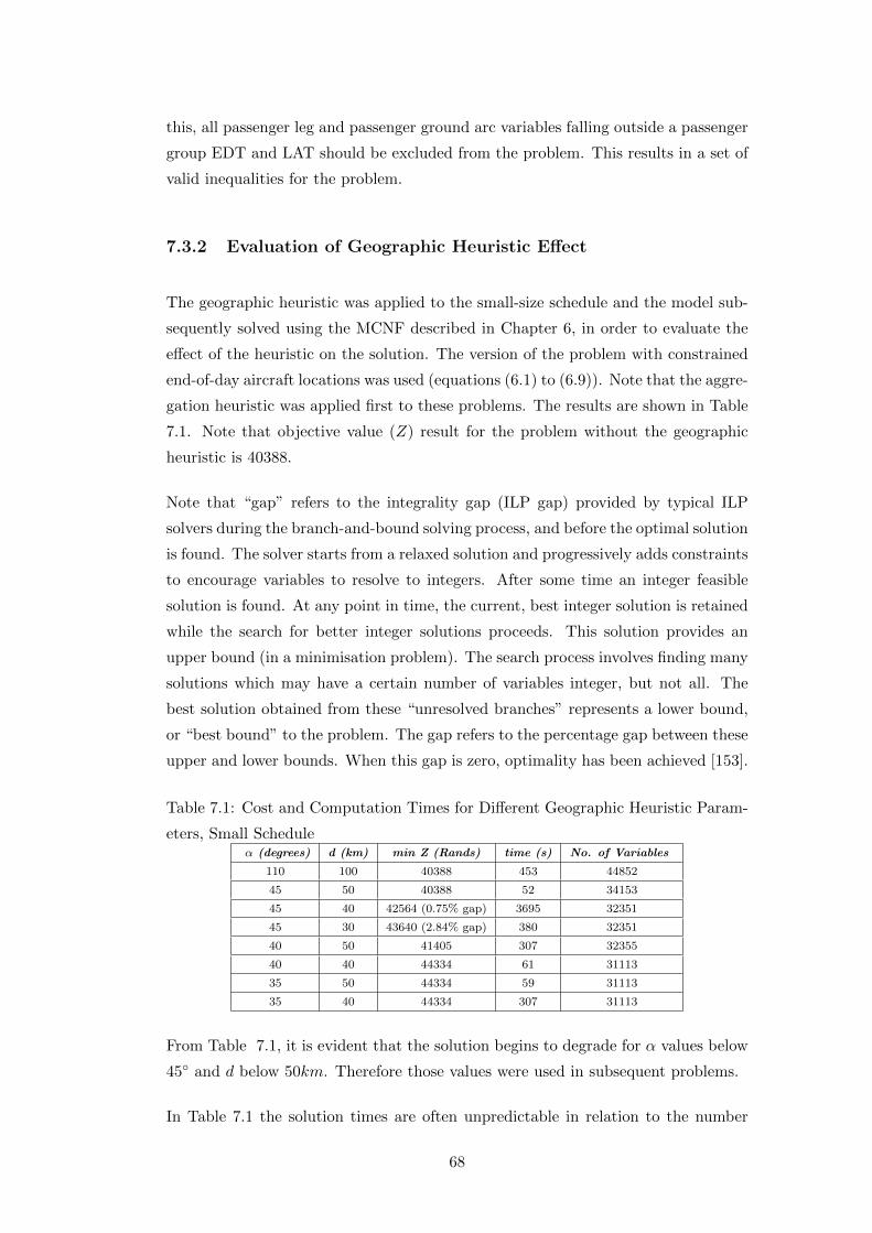
this, all passenger leg and passenger ground arc variables falling outside a passenger
group EDT and LAT should be excluded from the problem. This results in a set of
valid inequalities for the problem.
7.3.2 Evaluation of Geographic Heuristic Effect
The geographic heuristic was applied to the small-size schedule and the model sub-
sequently solved using the MCNF described in Chapter 6, in order to evaluate the
effect of the heuristic on the solution. The version of the problem with constrained
end-of-day aircraft locations was used (equations (6.1) to (6.9)). Note that the aggre-
gation heuristic was applied first to these problems. The results are shown in Table
7.1. Note that objective value (Z) result for the problem without the geographic
heuristic is 40388.
Note that “gap” refers to the integrality gap (ILP gap) provided by typical ILP
solvers during the branch-and-bound solving process, and before the optimal solution
is found. The solver starts from a relaxed solution and progressively adds constraints
to encourage variables to resolve to integers. After some time an integer feasible
solution is found. At any point in time, the current, best integer solution is retained
while the search for better integer solutions proceeds. This solution provides an
upper bound (in a minimisation problem). The search process involves finding many
solutions which may have a certain number of variables integer, but not all. The
best solution obtained from these “unresolved branches” represents a lower bound,
or “best bound” to the problem. The gap refers to the percentage gap between these
upper and lower bounds. When this gap is zero, optimality has been achieved [153].
Table 7.1: Cost and Computation Times for Different Geographic Heuristic Param-
eters, Small Scheduleα (degrees) d (km) min Z (Rands) time (s) No. of Variables
110 100 40388 453 44852
45 50 40388 52 34153
45 40 42564 (0.75% gap) 3695 32351
45 30 43640 (2.84% gap) 380 32351
40 50 41405 307 32355
40 40 44334 61 31113
35 50 44334 59 31113
35 40 44334 307 31113
From Table 7.1, it is evident that the solution begins to degrade for α values below
45◦ and d below 50km. Therefore those values were used in subsequent problems.
In Table 7.1 the solution times are often unpredictable in relation to the number
68
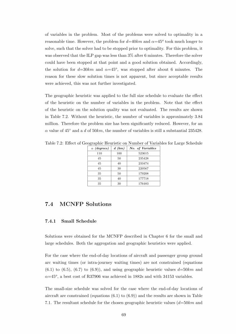
of variables in the problem. Most of the problems were solved to optimality in a
reasonable time. However, the problem for d=40km and α=45o took much longer to
solve, such that the solver had to be stopped prior to optimality. For this problem, it
was observed that the ILP gap was less than 3% after 6 minutes. Therefore the solver
could have been stopped at that point and a good solution obtained. Accordingly,
the solution for d=30km and α=45o, was stopped after about 6 minutes. The
reason for these slow solution times is not apparent, but since acceptable results
were achieved, this was not further investigated.
The geographic heuristic was applied to the full size schedule to evaluate the effect
of the heuristic on the number of variables in the problem. Note that the effect
of the heuristic on the solution quality was not evaluated. The results are shown
in Table 7.2. Without the heuristic, the number of variables is approximately 3.84
million. Therefore the problem size has been significantly reduced. However, for an
α value of 45◦ and a d of 50km, the number of variables is still a substantial 235428.
Table 7.2: Effect of Geographic Heuristic on Number of Variables for Large Scheduleα (degrees) d (km) No. of Variables
110 100 523615
45 50 235428
45 40 233474
45 30 220567
35 50 179208
35 40 177718
35 30 176483
7.4 MCNFP Solutions
7.4.1 Small Schedule
Solutions were obtained for the MCNFP described in Chapter 6 for the small and
large schedules. Both the aggregation and geographic heuristics were applied.
For the case where the end-of-day locations of aircraft and passenger group ground
arc waiting times (or intra-journey waiting times) are not constrained (equations
(6.1) to (6.5), (6.7) to (6.9)), and using geographic heuristic values d=50km and
α=45o, a best cost of R37906 was achieved in 1882s and with 34153 variables.
The small-size schedule was solved for the case where the end-of-day locations of
aircraft are constrained (equations (6.1) to (6.9)) and the results are shown in Table
7.1. The resultant schedule for the chosen geographic heuristic values (d=50km and
69

α=45o) is shown in Table 7.3. Note that the passenger groups referred to in the
table are aggregated groups, hence there are 26 groups listed.
The passenger groups which experience multiple flight legs and those which are
required to swap aircraft during their journey are shown in Table 7.4. The schedule
cost was R40388.
Note that the groups listed in column 1 of Table 7.4 are the only groups that ex-
perienced a journey which consisted of more than one flight leg. For example, row
1 shows that passenger group 7 consists of two passengers, and their journey from
origin to destination involved 3 aircraft flights. The last column shows that the
aircraft on which they were placed was a C206, and they started at location 2, went
to location 6, then location 4, then ended their journey at location 3.
Four passenger groups (15, 14, 21 and 19) needed to change aircraft and one group
changed aircraft twice and endured a total of 390 minutes (6.5 hours) of ground
waiting time en-route. Another group had to endure a wait of 580 minutes (9.7
hours) between flight legs.
The amount of intra-journey ground waiting time on multi-leg journeys was then
limited to turn around time only (i.e. 10 minutes per stop) by adding the constraint
shown in equation (6.10) to the problem. The result (using d=50km, α=45o) was a
schedule cost of R41338, using 34135 variables and 1462s solution time. Allowing 40
minutes of en-route ground waiting time (excluding 10 minutes turn around time per
stop) produced a schedule cost of R41300. With this constraint restricting ground
waiting times to the minimum (turn around times only), 5 passenger groups needed
to change aircraft en-route (Table 7.5). One group needed to change aircraft twice.
A summary of these results is included in Table 7.6. It was found that the problems
with both the end-of-day aircraft position constraints and the ground time limiting
constraints took excessively long and therefore impractical times to solve, hence
those results are not included in the table.
The effect of the aggregation heuristic was evaluated by solving the problem without
using this heuristic, and limiting the ground arc waiting time for passenger groups
to the minimum (using d=50km, α=45o, equations (6.1) to (6.10)). The result
was a schedule with a cost of R41907 with a 2.5% gap after 69329s (19.3hrs) of
processing time, and using 77089 variables. This is similar to R41338 obtained for
the aggregated instance (taking into account the 2.5% ILP gap).
When the non-aggregated model was executed with unlimited passenger ground
70

time, a schedule cost of R40388 resulted (0.7% ILP gap) after 56324s (15.6 hours)
processing using 77089 variables. This is identical to the R40388 obtained for the
aggregated instance. The large-size schedule could not be solved in non-aggregated
form due to the number of variables involved.
Table 7.3: Small Schedule SolutionOrigin Departure Destination Arrival Passenger Groups
Fleet Type Location Time∗ Location Time∗ on Board∗∗
C206 3 370 4 420 19
4 420 7 470 3
7 530 2 570 0
2 610 6 640 7
6 670 4 700 7, 14, 15
4 700 3 750 7
3 760 5 820 6
5 820 6 860 5
6 860 2 890 21
2 950 7 990 0
C206 7 380 6 410 0
6 480 3 560 4
3 610 1 650 0
1 660 3 700 21
3 810 4 860 22
4 860 3 910 2, 14
C206 7 460 2 500 11
2 500 7 540 10
7 870 2 910 20
2 950 7 990 0
7 950 4 1000 9, 18
4 1000 7 1050 16, 19
C208 7 370 6 390 15
6 420 3 480 23
3 720 4 760 1, 21
4 830 6 860 8, 17, 21
6 860 7 880 8, 13, 17
C208 7 420 6 440 12, 14
6 440 3 500 26
3 720 5 770 25
5 830 6 860 24
∗ Times are given in minutes in the day, i.e. 370 = 6h10, 420 = 7h00 ∗∗ 0 indicates empty aircraft flight
Table 7.4: Multi-Leg Trips - Unlimited Ground Waiting Time, Small SchedulePassenger No. of
Groups Passengers No. of Legs Fleet Type and Journey Sequence
7 2 3 C206: 2 - 6 - 4 - 3
15 1 2 C208: 7 - 6, wait: 480min, C206: 6 - 4
14 1 3 C208: 7 - 6, wait: 230min, C206: 6 - 4, wait: 160min, C206: 4 - 3
21 3 4 C206: 1 - 3, wait: 20min, C208: 3 - 4 - 6, C206: 6 - 2
19 2 2 C206: 3 - 4, wait: 580min, C206: 4 - 7
8 2 2 C208: 4 - 6 - 7
17 1 2 C208: 4 - 6 - 7
71
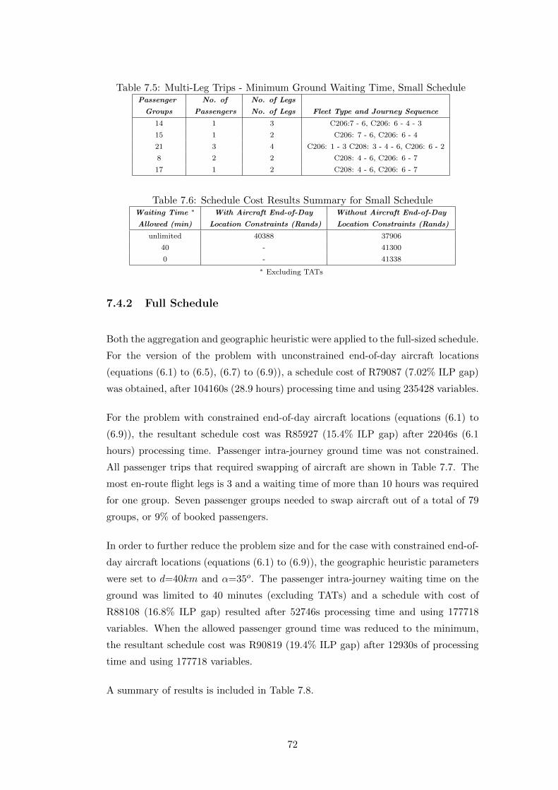
Table 7.5: Multi-Leg Trips - Minimum Ground Waiting Time, Small SchedulePassenger No. of No. of Legs
Groups Passengers No. of Legs Fleet Type and Journey Sequence
14 1 3 C206:7 - 6, C206: 6 - 4 - 3
15 1 2 C206: 7 - 6, C206: 6 - 4
21 3 4 C206: 1 - 3 C208: 3 - 4 - 6, C206: 6 - 2
8 2 2 C208: 4 - 6, C206: 6 - 7
17 1 2 C208: 4 - 6, C206: 6 - 7
Table 7.6: Schedule Cost Results Summary for Small ScheduleWaiting Time ∗ With Aircraft End-of-Day Without Aircraft End-of-Day
Allowed (min) Location Constraints (Rands) Location Constraints (Rands)
unlimited 40388 37906
40 - 41300
0 - 41338
∗ Excluding TATs
7.4.2 Full Schedule
Both the aggregation and geographic heuristic were applied to the full-sized schedule.
For the version of the problem with unconstrained end-of-day aircraft locations
(equations (6.1) to (6.5), (6.7) to (6.9)), a schedule cost of R79087 (7.02% ILP gap)
was obtained, after 104160s (28.9 hours) processing time and using 235428 variables.
For the problem with constrained end-of-day aircraft locations (equations (6.1) to
(6.9)), the resultant schedule cost was R85927 (15.4% ILP gap) after 22046s (6.1
hours) processing time. Passenger intra-journey ground time was not constrained.
All passenger trips that required swapping of aircraft are shown in Table 7.7. The
most en-route flight legs is 3 and a waiting time of more than 10 hours was required
for one group. Seven passenger groups needed to swap aircraft out of a total of 79
groups, or 9% of booked passengers.
In order to further reduce the problem size and for the case with constrained end-of-
day aircraft locations (equations (6.1) to (6.9)), the geographic heuristic parameters
were set to d=40km and α=35o. The passenger intra-journey waiting time on the
ground was limited to 40 minutes (excluding TATs) and a schedule with cost of
R88108 (16.8% ILP gap) resulted after 52746s processing time and using 177718
variables. When the allowed passenger ground time was reduced to the minimum,
the resultant schedule cost was R90819 (19.4% ILP gap) after 12930s of processing
time and using 177718 variables.
A summary of results is included in Table 7.8.
72

Table 7.7: Multiple Leg Trips for Large SchedulePassenger Groups No. of Passengers No. of Legs Fleet Type and Journey Sequence
30, 31, 32 3 4 C206:1 - 3, C208: 3 - 4 - 6 C206: 6 - 2
8 3 3 C206: 2 - 6 - 4 - 3
19 1 3 C208: 7 - 6 C206: 6 - 4 - 3
25, 27 2 2 C206: 3 - 4 wait: 610 minutes C206: 4 - 7
21 1 2 C208: 7 - 6 C206: 6 - 4
9 2 2 C208: 4 - 6 - 7
23 1 2 C208: 4 - 6 - 7
Table 7.8: Schedule Cost Results Summary for Large ScheduleHeuristic Waiting Time With Aircraft End-of-Day Without Aircraft End-of-Day
Values Allowed (min) Location Constraints (Rands) Location Constraints (Rands)
d=50, α=45 unlimited 85927 (15.4% gap) 79087 (7.02% gap)
d=40, α=35 40 88108 (16.8% gap) -
d=40, α=35 0 90819 (19.4% gap) -
7.5 Discussion
From Table 7.1, the problem solution begins to degrade for values of d between
20 and 50, and values of α of between 25o and 45o. Therefore suitable values are
d=50km and α=45o and these values are used in further computations. Notable
is the fact that a substantially reduced problem size (31%) can be achieved with
tighter geographic heuristic parameters with only a 9.8% reduction in optimality
when comparing the worst case calculated in Table 7.1 (schedule cost R44334) with
the best case (R40388).
The full schedule models produced numbers of variables exceeding 150 000 and as
such could not be solved to optimality in a reasonable time. It was found that the
ILP solver slowed down substantially as the ILP gap reduced, requiring many hours
of processing time to reduce the ILP gap to between 12% and 20%.
The full schedule solution with constrained end-of-day locations could be found to
a 15.4% gap after just over 6 hours, and produced a cost of R85927.
Although good solutions can be achieved using this method, the number of variables
generated is still too many for practical purposes for the full-size schedule, unless
specialised solution methods and/or processing hardware are developed. However,
the method will be practical for moderate size instances (up to 80 requests) of the
airline taxi problem.
It should be noted that this formulation (equations (6.1) to (6.9)) allows swapping of
groups between different aircraft. Adding constraints to prevent this would require
73

additional variables and constraints, increasing the problem size significantly and
increasing the solution computation time accordingly. Table 7.4 shows the groups
that experienced aircraft swapping and ground waits en-route for the small schedule,
including some unreasonably long waiting times. Therefore the additional constraint
(6.10) was added to limit passenger waiting times on the ground, and this raised
the cost of the schedules accordingly. The small schedule went from costing R37906
with unlimited passenger ground waiting time en-route, to R41338 with passenger
ground waiting time limited to the minimum. The passenger ground time limiting
constraints were observed to have a detrimental effect on processing times.
The constraints on passenger waiting times caused the schedule cost to increase. This
means the airline can save further costs by allowing increased sized time windows.
This might be possible with boxes and possibly with staff as well, but is unlikely to
be acceptable for many tourist groups.
For the small schedule, limiting the passenger group ground time to the minimum
reduced the number of groups that experienced multi-leg trips from 7 (27%) to 5
(19%) out of 26 total groups (Table 7.5). However, for unlimited passenger ground
time, 4 groups swapped aircraft (15%) vs 5 groups (19%) for the case where ground
time was limited to the minimum. For the full-sized schedule, only 11% of passengers
needed to swap aircraft.
There are various options open to the airline in terms of quality of service and using
this modelling technique. The easiest way to control quality of service provided will
be to limit the EDT and LAT (time windows) of all passenger groups which need
a higher quality of service than others, e.g. tourist groups vs employees and boxes.
Providing tight time windows will reduce multi-leg journeys and aircraft swapping.
A further option is to provide passengers with a two-tier pricing structure, where
the lower tier has flexible pick-up and delivery times and may be subject to long
ground waiting times. This would remove the need for some of the passenger ground
time limiting constraints which slow the processing time down.
The small schedule was used to evaluate the effect of the aggregation heuristic. The
version of the problem without aggregated groups and with zero passenger ground
waiting time produced a cost of R41907 but could only be solved with a 2.5% ILP
gap in a reasonable processing time. This compares favourably with the aggregated
version of the problem, which produced a schedule cost of R41338, and suggests the
aggregation heuristic has a marginal, if any, effect on the quality of the solutions.
Even though the number of variables in the non-aggregated model is not excessive
74

(77089), the solution times are long. This is due to there being substantially fewer
solutions in close proximity in the feasible region in the case of the aggregated model,
therefore the branch-and-bound process is far more efficient in pruning.
Although the number of variables was high and processing time long for the full
schedule using the MCNF with TD method, good solutions can be obtained. The
process speed can be increased by making the TDs longer, by shortening the day,
or by tightening the geographic heuristic. The method would be appropriate for
smaller instances of this problem.
In terms of portability of the heuristics, both could be applied to certain PDP type
VRPs. It is reasonable to assume the geographic heuristic will be applicable to the
DARP and other paired PDPs, and can be combined with other construction and
improvement methods.
75
8 Agent Routing Variable Generation
8.1 Description
The ILP with time discretisations is theoretically limited in terms of optimality of
solution by the use of time steps, since aircraft are limited to taking off and arriving
only at the nodes associated with a time step. Continuous variable node times would
be preferable to the use of time steps, but the formulation becomes too complicated,
with a substantial number of constraints, and is unwieldy for problems of the size
considered in this work.
An alternative method of obtaining nodes which may be better placed in time for
improved solutions is by using simulation-type agents to generate routes and thereby
also generate node times. Ant colony optimisation (ACO) also utilises agents which
use random search to generate routes, but generally is used for simpler, less con-
strained problems ([154], [61], [60]).
A method related to random search, but without the learning capability of ACO,
was devised for this problem. Effectively agents are allowed to search for feasible
or partially-feasible solutions. The solutions obtained are used to generate well-
positioned nodes and good legs for a mixed integer linear programming (MILP)
formulation. The quality of the solution will then depend on how long the agents
are given to search. If no good solution is found, an iterative improvement procedure
is proposed.
The method described here involves allowing agents (effectively aircraft) to start
at the beginning of the day and route themselves through to the end of the day,
collecting and delivering as many groups as possible. At the start of each leg, the
aircraft must decide where it should fly to, or whether it should stay at its current
location. The aircraft considers flying to each possible destination in turn and
assigns an attraction measure to each of these possible locations. A filter ensures
that locations which have no reason to be visited by the aircraft are assigned a zero
76
attractiveness value and therefore cannot be selected. The attractiveness of any
location is based on eight factors:
• The distance to the location.
• The available seats in the aircraft.
• Whether there are any groups waiting at the location and whether there is
space in the aircraft to accommodate them.
• How close the arrival time of the aircraft would be to the waiting groups’ EDT.
• Whether those waiting groups have similar destinations to any groups which
are already on board the aircraft.
• If there are any on-board groups, whether their destination is the location
under consideration.
• Whether the aircraft could fly to the location under consideration, then still
deliver all of the on-board groups on time.
• The size of the waiting group.
If a location has no waiting groups, and if there are no passengers on board with des-
tinations matching that location, the attractiveness of that location is automatically
set to zero.
After an attractiveness is assigned to every possible location, a Monte Carlo sampling
procedure is used to randomly select a location to fly to.
The aircraft is then moved to the new location and must decide which waiting groups
to collect there. If all waiting passengers cannot fit on board the aircraft, another
Monte Carlo selection process is used to choose which passenger groups should be
taken on board. The aircraft must then again decide which new location to fly to, or
whether it should wait on the ground for other passenger groups to become available
for collection.
This procedure was written in MATLAB and is included in Appendix D.
Nine parameters were included in the model to be used to adjust how attractive
each factor is (or to weigh the importance of the factor). These parameters were:
1. Difference between current time and LAT of on-board groups.
77
2. Number of on-board groups who have a destination matching the candidate
groups’ location (where candidate groups are groups waiting at the candidate
location to be picked up).
3. For the candidate groups, the difference between arrival time and EDT.
4. The geographical distance.
5. The number of on-board groups with destinations matching those of waiting
groups.
6. A parameter to increase the attractiveness of a location which is the destination
of a group taken on board, when considering taking another group on board
at the same location.
7. When at a location and having picked up at least one group, a parameter to
add attractiveness to take off without taking on any more waiting groups at
that location.
8. The time difference between the arrival time at the candidate location and the
time at which the aircraft will be forced to prioritise on-board groups which
must be delivered before their LAT.
9. The sizes of the candidate groups.
These parameters can be used to strictly enforce feasibility, or to allow some flexi-
bility in terms of group EDTs and LATs. More flexibility would widen the search.
Parameters to provide values for the attractiveness of the geographical distance and
the times were based on an exponential distribution. For example, the geographic
distance attractiveness was calculated as 1/ed/F1 , where d is the distance in kilome-
ters and F1 is the factor giving weight to the overall attractiveness. The exponential
distribution was used since it allows for a maximum upper limit and decays rapidly
initially. It is often used in other applications such as neural networks where weights
are required. In this application it proved to work adequately. However, in future
work, Gaussian and linear functions could also be investigated.
A penalty cost is given to undelivered schedule items such that the agent routing
function can be optimised with regards to cost. This was set at 10000.
Initially, the agent scheduling procedure is executed with no randomness, i.e. the
agent is always routed to the most attractive destination. The attractiveness param-
eters are then adjusted to obtain the best schedule result under these conditions. In
78
this process, an optimisation method can be used. For this work, the pattern search
optimisation method as supplied with MATLAB Global Optimization Toolbox was
applied [155]. The MATLAB pattern search algorithm is effectively a multi-variable
hill climbing technique, and as such, may return results from local optima.
Significantly, the best results were achieved when higher relative weighting was given
to the waiting group sizes than the other factors. The chosen factor values are shown
in Appendix D.
The procedure was then executed using randomness, ie, using Monte Carlo sampling
to select a destination at each decision point with weights based on the calculated
attractiveness of the possible locations.
The method was used to generate a number of schedules with unconstrained end-
of-day fleet locations. Most of the schedules thus generated were not feasible, since
the aircraft were all used up without all of the groups on the schedule having been
delivered. The routes generated by the schedule were used to create the nodes and
legs in the same type of formulation as described previously in Chapter 6, but with
some modifications. Because all of the flight leg variables thus introduced already
had times associated with them, there was no need for time discretisations. Also,
the constraint ensuring all groups were delivered to their respective destinations
was softened by removing it from the constraints and including it in the objective
function. This was done by adding a number to the objective function for every
group correctly delivered (on time and at the correct destination), then maximising
the objective. This number is subsequently referred to as the group delivery benefit
parameter.
This number, which can be interpreted as the maximum cost allowable for a passen-
ger leg, is used as the revenue (negative cost) coefficient for each passenger ground
arc which represents a passenger group reaching their destination on time. An al-
ternative is to use the maximum cost allowable for delivery of a single passenger,
in which case larger passenger groups (and hence tourist groups) would be favoured
for delivery over single passengers.
Since the objective of this model is to maximise the number of groups delivered, the
problem objective function is now maximised. The cost of each leg is still included
in the objective function.
This technique ensured that, in the case that insufficient variables were available
to obtain a good solution, the model could leave out the most expensive groups to
79
be delivered. Then, new legs could be introduced to the model in order to reduce
the cost of those deliveries, and the problem solved again. This process could be
repeated as many times as required until a suitably low-cost solution was found.
For this work, in the case that a suitably low-cost schedule could not be found which
delivered all of the groups in the first iteration, additional legs were added to the
problem in subsequent iterations as follows:
1. Consider each of the undelivered groups sequentially.
2. Add a leg from the origin of the group at EDT to the destination for all feasible
aircraft types.
3. Add the associated legs from each location in the geographic network of the
group to the origin at EDT.
4. Add the associated legs from the destination at arrival time to every other
location in the geographic network of the group.
5. Repeat the above process (2-4) for:
• A leg from the groups’ latest possible departure from the origin to the
destination.
• Legs placed at intervals of 20 minutes (or less) in between the origin at
EDT and the latest possible departure from the origin to the destination.
The effectiveness of this iterative process is dependent on the above-described method
of adding additional legs to the problem to aid a lower cost solution. It therefore
makes sense, as is done above, to supply legs to and from the origin and destination
of undelivered (i.e. expensive to deliver) passenger groups. If, after an iteration,
an improved solution is not obtained, the legs described can be added at shorter
intervals, or legs can be added from and to other locations and times.
Clearly, the problem will grow in magnitude after each iteration, so carrying out
the above procedure for more than four unscheduled groups was found to cause the
problem solution process to slow significantly. This is apparently not due to the
number of variables, since the number of variables never exceeded 60 000. Since the
solution suffers from slow ILP gap reduction as the gap becomes small, the effect is
most likely due to more solutions being introduced to the problem near the optimum
which are difficult to prune in the branch and bound process. One resolution is to
simply stop the solver at a small enough ILP gap.
80

Note that the heuristics developed in Chapter 7 are applicable here and were used
with similar setup parameters as was used for the MCNFP in Chapter 6.
A reasonable measure of the solution quality would be the load factor. This was
calculated by taking the load factors for each flight leg (number of occupied seats
divided by aircraft capacity) and multiplying them by the flying time for the leg.
These load factors are added for all the legs in a schedule, and divided by the total
schedule flying time. However, for this work and for the problem instance under
consideration, the minimum cost per group delivery was known to be just over
R1000 per group. Therefore this number (cost per group delivery) was used as a
performance measure and target. A similar value could most likely be used for other
instances of the problem.
The number to be deducted from the objective function for each delivered group
(group delivery benefit parameter) can be adjusted to encourage more or less groups
to be delivered in any iteration, thus ensuring only the most expensive groups are
excluded from the solution.
The problem solution was found to produce a number of incidents of aircraft swap-
ping, as well as some wait times which may be considered too long. To counter
this effect, the objective function was modified with a cost per minute of time for
each passenger group. This was achieved by calculating the time taken for each leg
(Ry) and including it as the cost coefficient for each passenger leg variable yxg (see
equation (8.1)), and similarly, adding the time taken (Rt) for each passenger ground
arc t to the cost in the objective function. The resultant MCNF model is as follows:
The objective is to maximize the number of groups delivered while deducting costs:
maximise∑g∈G
BEN tnlg −∑y∈Y
Ryy −∑t∈T
Rtt−∑x∈X
Cxx (8.1)
where tnlg is the passenger group ground arc with start node corresponding to LAT
and destination for passenger group g. There will be one tnlg for each group. BEN
is the group delivery benefit parameter (or maximum cost per group delivered).
Note that one could easily make this parameter the maximum cost per passenger
delivered if required, by multiplying the size of the group to this term. Ry and Rt are
the times associated with passenger leg y and passenger ground arc t respectively.
As before, Cx is the cost associated with the flight variable x.
The aircraft node conservation of flow constraints are as follows:
81
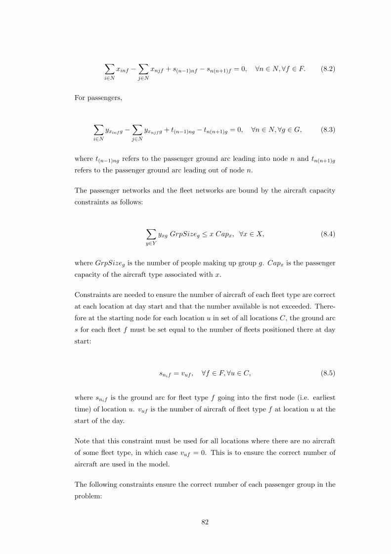
∑i∈N
xinf −∑j∈N
xnjf + s(n−1)nf − sn(n+1)f = 0, ∀n ∈ N, ∀f ∈ F. (8.2)
For passengers,
∑i∈N
yxinfg −∑j∈N
yxnjfg + t(n−1)ng − tn(n+1)g = 0, ∀n ∈ N, ∀g ∈ G, (8.3)
where t(n−1)ng refers to the passenger ground arc leading into node n and tn(n+1)g
refers to the passenger ground arc leading out of node n.
The passenger networks and the fleet networks are bound by the aircraft capacity
constraints as follows:
∑y∈Y
yxg GrpSizeg ≤ x Capx, ∀x ∈ X, (8.4)
where GrpSizeg is the number of people making up group g. Capx is the passenger
capacity of the aircraft type associated with x.
Constraints are needed to ensure the number of aircraft of each fleet type are correct
at each location at day start and that the number available is not exceeded. There-
fore at the starting node for each location u in set of all locations C, the ground arc
s for each fleet f must be set equal to the number of fleets positioned there at day
start:
snif = vuf , ∀f ∈ F,∀u ∈ C, (8.5)
where snif is the ground arc for fleet type f going into the first node (i.e. earliest
time) of location u. vuf is the number of aircraft of fleet type f at location u at the
start of the day.
Note that this constraint must be used for all locations where there are no aircraft
of some fleet type, in which case vuf = 0. This is to ensure the correct number of
aircraft are used in the model.
The following constraints ensure the correct number of each passenger group in the
problem:
82
tnig = bug, ∀g ∈ G, ∀u ∈ C, (8.6)
where tnig is the passenger group ground arc with end node corresponding to the
first node at location u and bug is either 1 or zero, depending on whether u is the
origin for g.
The following constraints ensure passenger groups are at the correct locations at the
passenger group EDT :
tneg = 1, ∀g ∈ G, (8.7)
where tneg is the passenger group ground arc with end node corresponding to EDT
and origin for passenger group g.
The modelling process is shown schematically in a flowchart in Figure 8.1. The
process begins with application of the aggregation heuristic, which, in this case, ef-
fectively halves the booking list size. Thereafter the reduced booking list is presented
to the agents which intelligently and randomly produce a number of schedules. Vari-
able information is extracted from these schedules for the problem. The geographic
heuristic is then applied, and the model assembled and solved. If some groups are
not delivered, more variables must be added to the problem and the problem re-
assembled and resolved (an iteration). The delivery benefit parameter can also be
increased to encourage more group deliveries, but at an increased cost per group.
This process is repeated until all groups are delivered at an acceptable cost.
8.2 Observations and Results
Ten schedules were randomly generated using the agent scheduling technique de-
scribed. The parameters relating to the legs were extracted from these schedules
and were used to generate variables to describe the MCNFP (nodes, arcs, etc). The
variables were then used in the ILP. This was done using three different values for
the group delivery benefit parameter in the objective function, in three different
solution schedules, as follows:
1. 2000, two iterations.
2. 1500, two iterations.
83
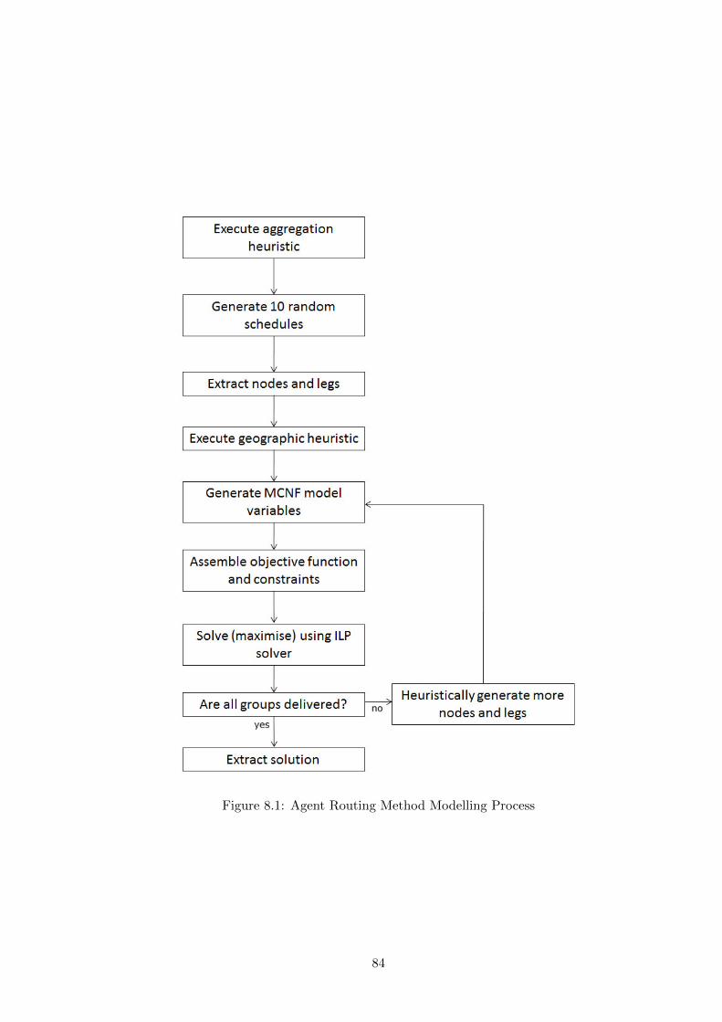
Figure 8.1: Agent Routing Method Modelling Process
84
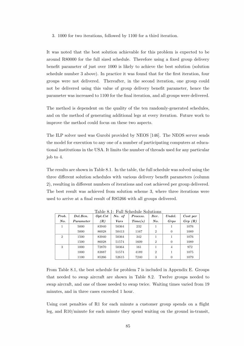
3. 1000 for two iterations, followed by 1100 for a third iteration.
It was noted that the best solution achievable for this problem is expected to be
around R80000 for the full sized schedule. Therefore using a fixed group delivery
benefit parameter of just over 1000 is likely to achieve the best solution (solution
schedule number 3 above). In practice it was found that for the first iteration, four
groups were not delivered. Thereafter, in the second iteration, one group could
not be delivered using this value of group delivery benefit parameter, hence the
parameter was increased to 1100 for the final iteration, and all groups were delivered.
The method is dependent on the quality of the ten randomly-generated schedules,
and on the method of generating additional legs at every iteration. Future work to
improve the method could focus on these two aspects.
The ILP solver used was Gurobi provided by NEOS [146]. The NEOS server sends
the model for execution to any one of a number of participating computers at educa-
tional institutions in the USA. It limits the number of threads used for any particular
job to 4.
The results are shown in Table 8.1. In the table, the full schedule was solved using the
three different solution schedules with various delivery benefit parameters (column
2), resulting in different numbers of iterations and cost achieved per group delivered.
The best result was achieved from solution scheme 3, where three iterations were
used to arrive at a final result of R85266 with all groups delivered.
Table 8.1: Full Schedule SolutionsProb. Del.Ben. Opt.Cst No. of Process. Iter. Undel. Cost per
No. Parameter (R) Vars Time(s) No. Grps Grp (R)
1 5000 83940 50364 232 1 1 1076
5000 86028 50413 1167 2 0 1089
2 1500 83940 50364 342 1 1 1076
1500 86028 51574 1609 2 0 1089
3 1000 72870 50364 161 1 4 972
1000 83887 51574 4189 2 1 1075
1100 85266 52615 7240 3 0 1079
From Table 8.1, the best schedule for problem 7 is included in Appendix E. Groups
that needed to swap aircraft are shown in Table 8.2. Twelve groups needed to
swap aircraft, and one of those needed to swap twice. Waiting times varied from 19
minutes, and in three cases exceeded 1 hour.
Using cost penalties of R1 for each minute a customer group spends on a flight
leg, and R10/minute for each minute they spend waiting on the ground in-transit,
85
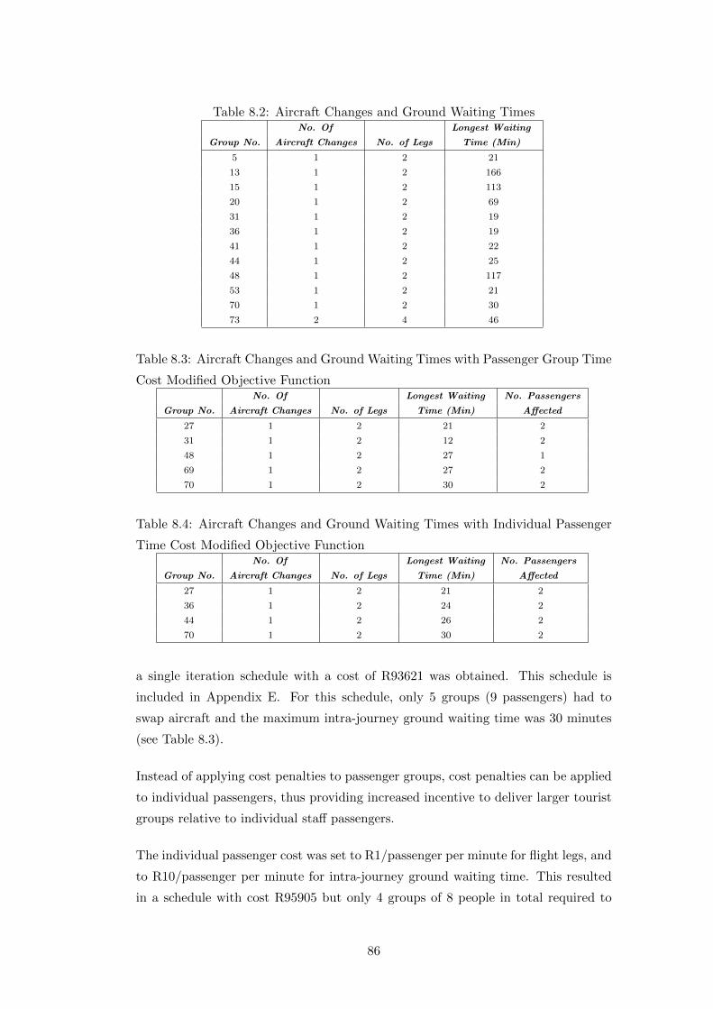
Table 8.2: Aircraft Changes and Ground Waiting TimesNo. Of Longest Waiting
Group No. Aircraft Changes No. of Legs Time (Min)
5 1 2 21
13 1 2 166
15 1 2 113
20 1 2 69
31 1 2 19
36 1 2 19
41 1 2 22
44 1 2 25
48 1 2 117
53 1 2 21
70 1 2 30
73 2 4 46
Table 8.3: Aircraft Changes and Ground Waiting Times with Passenger Group Time
Cost Modified Objective FunctionNo. Of Longest Waiting No. Passengers
Group No. Aircraft Changes No. of Legs Time (Min) Affected
27 1 2 21 2
31 1 2 12 2
48 1 2 27 1
69 1 2 27 2
70 1 2 30 2
Table 8.4: Aircraft Changes and Ground Waiting Times with Individual Passenger
Time Cost Modified Objective FunctionNo. Of Longest Waiting No. Passengers
Group No. Aircraft Changes No. of Legs Time (Min) Affected
27 1 2 21 2
36 1 2 24 2
44 1 2 26 2
70 1 2 30 2
a single iteration schedule with a cost of R93621 was obtained. This schedule is
included in Appendix E. For this schedule, only 5 groups (9 passengers) had to
swap aircraft and the maximum intra-journey ground waiting time was 30 minutes
(see Table 8.3).
Instead of applying cost penalties to passenger groups, cost penalties can be applied
to individual passengers, thus providing increased incentive to deliver larger tourist
groups relative to individual staff passengers.
The individual passenger cost was set to R1/passenger per minute for flight legs, and
to R10/passenger per minute for intra-journey ground waiting time. This resulted
in a schedule with cost R95905 but only 4 groups of 8 people in total required to
86

swap aircraft and a longest waiting time of 20 minutes (see Table 8.4). Using more
randomly-generated schedules (20 in total), 2 iterations were required to reduce this
cost to R87471 (R1107 per passenger group).
8.3 Discussion
Compared to the MCNF model from Chapter 6, the fewer variables generated by this
method make it more practical in that it solves faster while still providing acceptable
solutions. The use of a similar MCNF ILP formulation to that used in Chapter 6
means that swapping of aircraft may occur in the final solution. In this case, 12
groups (15%) needed to swap aircraft. Note that, in terms of service quality, the
same options are open to the airline for this method as for the previously described
method (Chapters 6 and 7).
If a cost is given to intra-journey waiting times for passengers and passenger legs,
the swapping of aircraft and length of ground times are positively affected. Options
are to apply a cost per passenger, per passenger group, or to apply a higher cost for
tourists and lower costs for boxes and staff. A cost could be added to the objective
function to encourage aircraft end-of-day locations, as opposed to using constraints.
The explanation of Tables 8.3 and 8.4 include demonstrations of how the costs can be
applied to the objective function to change operational characteristics of the solution.
In this case, when costs are applied to passenger time on an individual passenger
basis, slightly fewer passengers had to swap aircraft and wait, but the schedule cost
was higher. This cost was reduced by adding an additional 10 randomly generated
schedules and resolving.
This method provides flexibility, in that it could easily be applied to all kinds of
routing problems. The only application consideration is how large the search area
is, as a smaller area (more tightly constrained problem) will be advantageous in
terms of solution quality.
87

9 Composite Variable Formulation
9.1 Description
An alternative method of solving the problem involves constructing composite vari-
ables as Ronen [137] describes. For this problem, the aircraft flight variables can be
combined with each other and with passenger flight variables, such that the resul-
tant variables provide feasible chains of flight legs which can be included as part of
a route in a schedule. The advantage of such a formulation is that it removes the
need to have separate passenger variables completely, vastly reducing the size of the
problem, since the passenger flight variables and passenger ground arc variables are
the largest component of the problem.
The procedure begins by applying the aggregation heuristic. Thereafter, the proce-
dure for creating the composite variables is as follows:
1. Create single flight variables: For every booking and every fleet type,
create a flight variable which can satisfy that booking. This means the aircraft
type capacity will be large enough to carry the passenger group, and the length
of the flight in terms of time will match the aircraft speed and the distance to
be flown.
2. Dual linking: For every single flight variable, search for other single flight
variables which can be joined on to it. This means the fleet types are similar,
the destination of the first variable matches the origin of the second variable
and the EDT and LAT for both variables will still be met. However, this is
only done in cases where at least one more booking could be satisfied by the
linked variable, in other words, at least a third passenger group can fit in the
aircraft (sufficient capacity) and will fly on both legs.
The process is shown graphically in Figure 9.1 in which three locations are
depicted. Two single flight variables have been found which can be joined,
88

since flight variable 1 has a destination (ABU) which coincides with the origin
of flight variable 2. Flight variable 1 transports passenger groups 3 and 5 from
HND to ABU. Flight variable 2 transports passenger groups 2 and 7 from ABU
to JAO. Both flight variable 1 and 2 have spare seats available. Therefore they
are linked together as shown to form a new, 2-leg flight variable. Then a search
is done to find other passenger groups that can be assigned to this new variable.
Any groups that have an origin HND and destination JAO and can fit in the
aircraft as it flies on the existing two legs will be considered. If no groups can
be found, the new variable is discarded. In the Figure, group 1 has been found
and assigned to the new variable. Therefore the new flight variable is added to
the problem. The existing single flight variables are retained in the problem.
flight 1
flight 2
Note: Numbers in parentheses refer to passenger groups
Figure 9.1: Linking of Two Flight Variables (Dual Linking)
3. Further linking: For every 2-link variable, search for single variables which
could be joined on to create 3 leg and more linked variables. Again, only
create such a variable if some other group or groups could also be assigned
to the resultant variable. This linking process can be repeated as many times
as required to create longer chains of flight variables. However, the problem
can quickly become large and unwieldy, and in such cases the process can be
stopped after 3 or 4 link variables have been created.
89
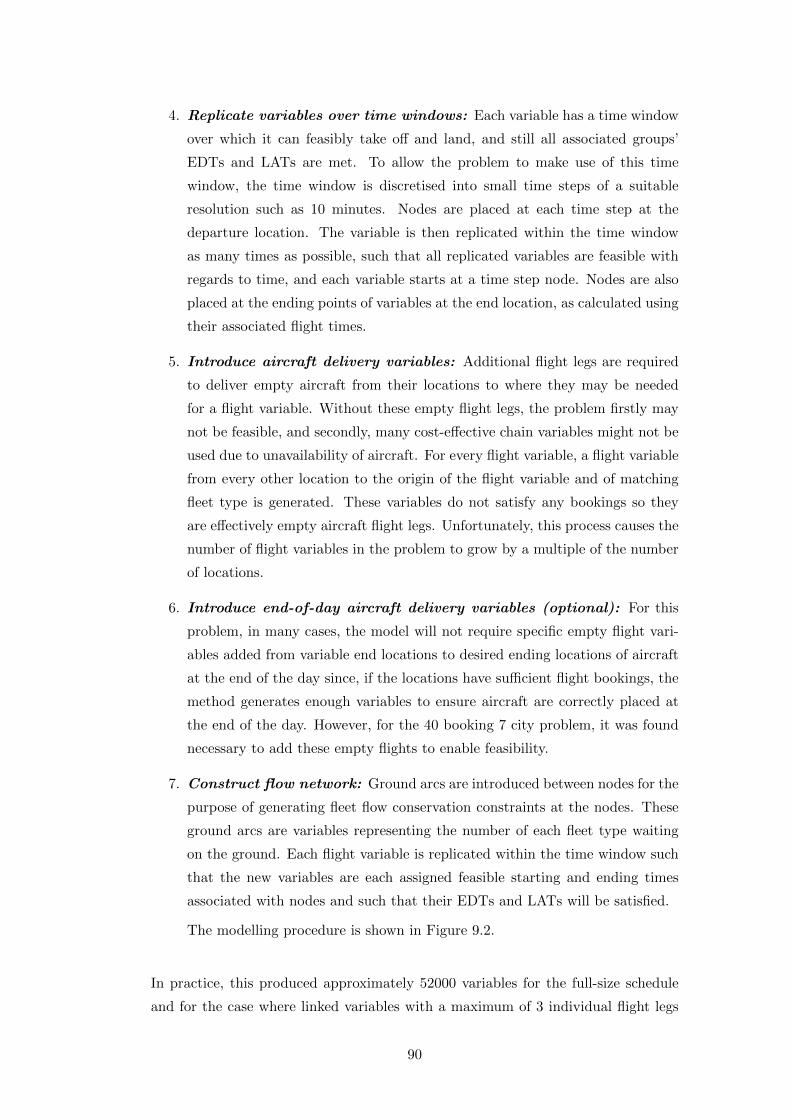
4. Replicate variables over time windows: Each variable has a time window
over which it can feasibly take off and land, and still all associated groups’
EDTs and LATs are met. To allow the problem to make use of this time
window, the time window is discretised into small time steps of a suitable
resolution such as 10 minutes. Nodes are placed at each time step at the
departure location. The variable is then replicated within the time window
as many times as possible, such that all replicated variables are feasible with
regards to time, and each variable starts at a time step node. Nodes are also
placed at the ending points of variables at the end location, as calculated using
their associated flight times.
5. Introduce aircraft delivery variables: Additional flight legs are required
to deliver empty aircraft from their locations to where they may be needed
for a flight variable. Without these empty flight legs, the problem firstly may
not be feasible, and secondly, many cost-effective chain variables might not be
used due to unavailability of aircraft. For every flight variable, a flight variable
from every other location to the origin of the flight variable and of matching
fleet type is generated. These variables do not satisfy any bookings so they
are effectively empty aircraft flight legs. Unfortunately, this process causes the
number of flight variables in the problem to grow by a multiple of the number
of locations.
6. Introduce end-of-day aircraft delivery variables (optional): For this
problem, in many cases, the model will not require specific empty flight vari-
ables added from variable end locations to desired ending locations of aircraft
at the end of the day since, if the locations have sufficient flight bookings, the
method generates enough variables to ensure aircraft are correctly placed at
the end of the day. However, for the 40 booking 7 city problem, it was found
necessary to add these empty flights to enable feasibility.
7. Construct flow network: Ground arcs are introduced between nodes for the
purpose of generating fleet flow conservation constraints at the nodes. These
ground arcs are variables representing the number of each fleet type waiting
on the ground. Each flight variable is replicated within the time window such
that the new variables are each assigned feasible starting and ending times
associated with nodes and such that their EDTs and LATs will be satisfied.
The modelling procedure is shown in Figure 9.2.
In practice, this produced approximately 52000 variables for the full-size schedule
and for the case where linked variables with a maximum of 3 individual flight legs
90

Figure 9.2: Composite Variable Modelling Method
91
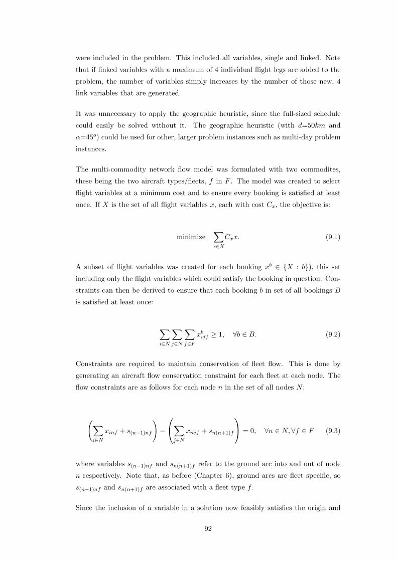
were included in the problem. This included all variables, single and linked. Note
that if linked variables with a maximum of 4 individual flight legs are added to the
problem, the number of variables simply increases by the number of those new, 4
link variables that are generated.
It was unnecessary to apply the geographic heuristic, since the full-sized schedule
could easily be solved without it. The geographic heuristic (with d=50km and
α=45o) could be used for other, larger problem instances such as multi-day problem
instances.
The multi-commodity network flow model was formulated with two commodites,
these being the two aircraft types/fleets, f in F . The model was created to select
flight variables at a minimum cost and to ensure every booking is satisfied at least
once. If X is the set of all flight variables x, each with cost Cx, the objective is:
minimize∑x∈X
Cxx. (9.1)
A subset of flight variables was created for each booking xb ∈ {X : b}), this set
including only the flight variables which could satisfy the booking in question. Con-
straints can then be derived to ensure that each booking b in set of all bookings B
is satisfied at least once:
∑i∈N
∑j∈N
∑f∈F
xbijf ≥ 1, ∀b ∈ B. (9.2)
Constraints are required to maintain conservation of fleet flow. This is done by
generating an aircraft flow conservation constraint for each fleet at each node. The
flow constraints are as follows for each node n in the set of all nodes N :
(∑i∈N
xinf + s(n−1)nf
)−
∑j∈N
xnjf + sn(n+1)f
= 0, ∀n ∈ N, ∀f ∈ F (9.3)
where variables s(n−1)nf and sn(n+1)f refer to the ground arc into and out of node
n respectively. Note that, as before (Chapter 6), ground arcs are fleet specific, so
s(n−1)nf and sn(n+1)f are associated with a fleet type f .
Since the inclusion of a variable in a solution now feasibly satisfies the origin and
92

destination requirements, as well as time window requirements, for all of the asso-
ciated passenger groups, no nodal conservation of passenger group flow constraints
are required.
Since each node has an associated location and time, the ground arc leading to the
first node at any location (i.e. with the earliest time) should be set to the number
of aircraft of that fleet type at that location at the start of the day:
snif = vuif , ∀u ∈ C,∀f ∈ F, (9.4)
where vuif is the number of aircraft starting at location u, and snif is the ground
arc for fleet type f going into the first node (earliest time) at location u.
Similarly, the ground arc leading from the last node of the day will represent the
number of aircraft at a particular destination at the end of the day, and can be
constrained if required:
snof = vuof , ∀u ∈ C,∀f ∈ F, (9.5)
where vuof is the number of aircraft ending at location u, and snof is the ground arc
for fleet type f going out of the last node (latest time) at location u.
9.2 Observations and Results
9.2.1 Small Schedule
The problem was executed with constrained end-of-day aircraft locations (i.e. in-
cluding equation (9.5)) and the maximum number of linked variables included in the
problem was varied from 3 to 5. The results are shown in Table 9.1. It was found
that no further linking occurred after variables with 4 links had been produced.
The best solution achieved (cost R44200) was 6.9% from the best solution using the
MCNF ILP with limited passenger group waiting time in Chapter 7 (cost R41338).
The resultant schedule is shown in Table 9.2. In this table, the group numbers refer
to the original, un-aggregated group numbers. Groups that appear on two different
aircraft have a choice of more than one leg. Thirty flights in total are used for the
schedule.
93
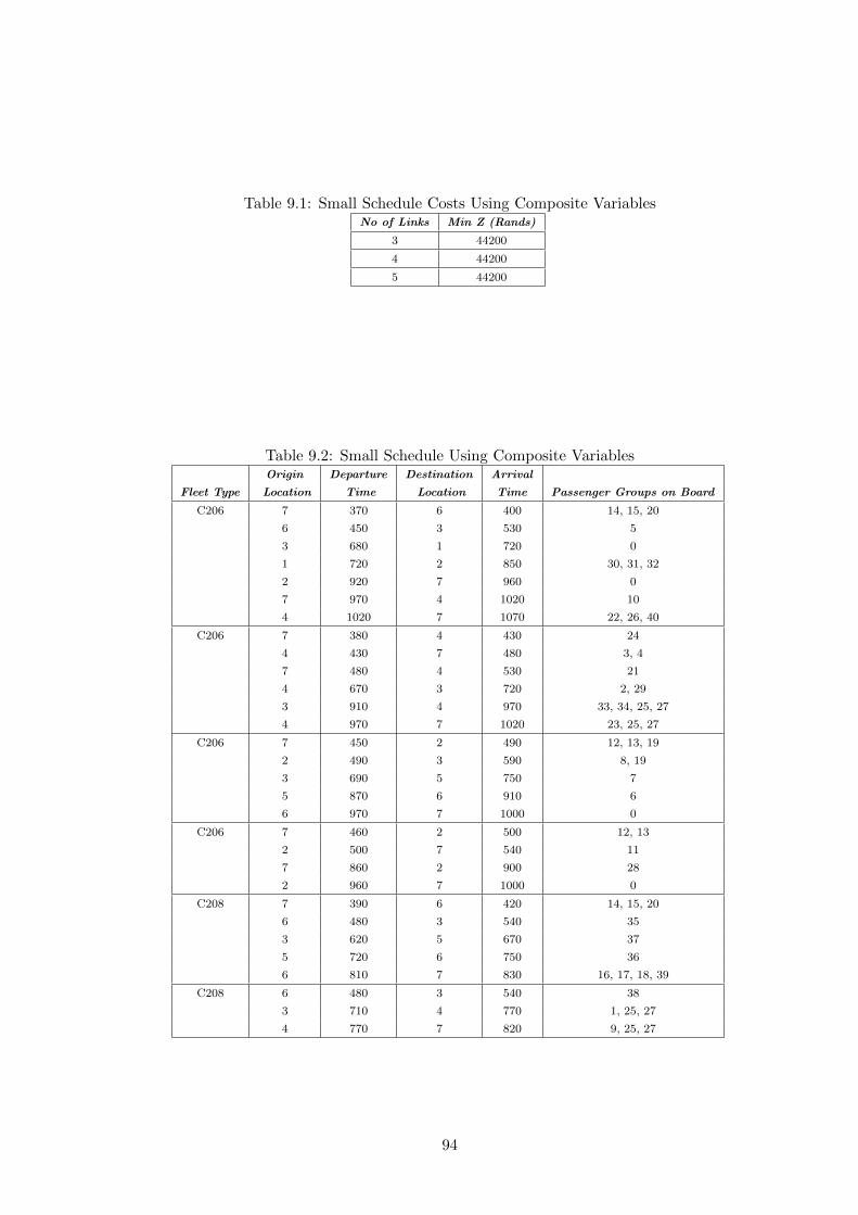
Table 9.1: Small Schedule Costs Using Composite VariablesNo of Links Min Z (Rands)
3 44200
4 44200
5 44200
Table 9.2: Small Schedule Using Composite VariablesOrigin Departure Destination Arrival
Fleet Type Location Time Location Time Passenger Groups on Board
C206 7 370 6 400 14, 15, 20
6 450 3 530 5
3 680 1 720 0
1 720 2 850 30, 31, 32
2 920 7 960 0
7 970 4 1020 10
4 1020 7 1070 22, 26, 40
C206 7 380 4 430 24
4 430 7 480 3, 4
7 480 4 530 21
4 670 3 720 2, 29
3 910 4 970 33, 34, 25, 27
4 970 7 1020 23, 25, 27
C206 7 450 2 490 12, 13, 19
2 490 3 590 8, 19
3 690 5 750 7
5 870 6 910 6
6 970 7 1000 0
C206 7 460 2 500 12, 13
2 500 7 540 11
7 860 2 900 28
2 960 7 1000 0
C208 7 390 6 420 14, 15, 20
6 480 3 540 35
3 620 5 670 37
5 720 6 750 36
6 810 7 830 16, 17, 18, 39
C208 6 480 3 540 38
3 710 4 770 1, 25, 27
4 770 7 820 9, 25, 27
94

9.2.2 Full Schedule
The full schedule was solved with constrained end-of-day aircraft locations (i.e. in-
cluding equation (9.5)) and the results are shown in Table 9.3. Column 1 in the
table refers to the maximum number of legs that were linked together to form a
variable. As longer linked variables are constructed and inserted into the problem,
the number of variables in the problem (column 2) increases accordingly. This is
because each time longer linked variables are generated, these additional variables
are simply added to all of the existing variables. The processing time (column 4)
also increases and the schedule cost decreases (column 3, “Min Z”).
Note that if a schedule is produced from variables that have a maximum number of
three links, no passenger group will have a trip of more than three aircraft legs.
Table 9.3: Full Schedule Costs Using Composite Variables with Constrained End-
Of-Day Aircraft LocationsMax. No. of Links No. of Variables Min Z (Rands) Processing Time (s)
2 42522 88230 18.1
3 52404 87756 32.9
4 61728 86787 251.9
5 82262 86787 665.4
The problem was solved with unconstrained end-of-day aircraft locations. This ver-
sion produced a schedule cost of R87683 for the problem including a maximum size
of 3 link variables (9.8s solution time). This solution cost is similar to that obtained
using the method described in Chapter 8 for the equivalent problem (R87471), but
has the advantage of no aircraft changes for passengers and is faster to solve (32.9s
vs more than 1 hour).
9.3 Discussion
From Table 9.3, the processing time increases and the schedule cost decreases as the
maximum allowable number of links increases.
The method solves quickly if the number of variables in the problem is limited.
The method can not accommodate swapping of aircraft and limits the amount of
passenger ground time en-route. This makes it ideal for this particular problem,
since a high quality of service can be maintained. The method retains flexibility
in allowing end-of-day aircraft positions to be constrained. Even without providing
95
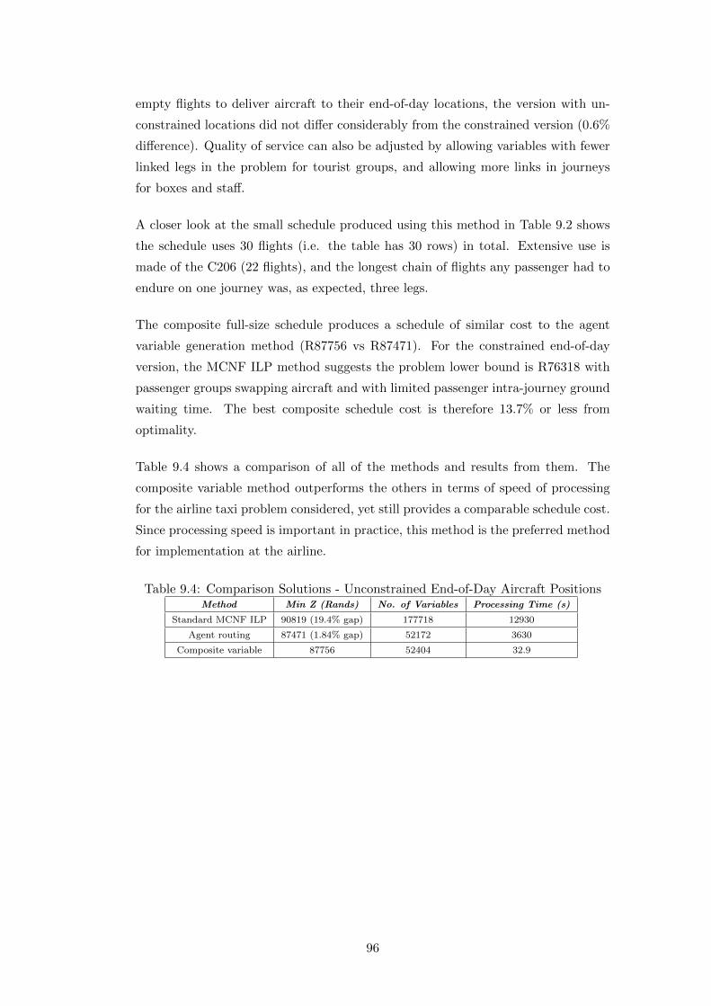
empty flights to deliver aircraft to their end-of-day locations, the version with un-
constrained locations did not differ considerably from the constrained version (0.6%
difference). Quality of service can also be adjusted by allowing variables with fewer
linked legs in the problem for tourist groups, and allowing more links in journeys
for boxes and staff.
A closer look at the small schedule produced using this method in Table 9.2 shows
the schedule uses 30 flights (i.e. the table has 30 rows) in total. Extensive use is
made of the C206 (22 flights), and the longest chain of flights any passenger had to
endure on one journey was, as expected, three legs.
The composite full-size schedule produces a schedule of similar cost to the agent
variable generation method (R87756 vs R87471). For the constrained end-of-day
version, the MCNF ILP method suggests the problem lower bound is R76318 with
passenger groups swapping aircraft and with limited passenger intra-journey ground
waiting time. The best composite schedule cost is therefore 13.7% or less from
optimality.
Table 9.4 shows a comparison of all of the methods and results from them. The
composite variable method outperforms the others in terms of speed of processing
for the airline taxi problem considered, yet still provides a comparable schedule cost.
Since processing speed is important in practice, this method is the preferred method
for implementation at the airline.
Table 9.4: Comparison Solutions - Unconstrained End-of-Day Aircraft PositionsMethod Min Z (Rands) No. of Variables Processing Time (s)
Standard MCNF ILP 90819 (19.4% gap) 177718 12930
Agent routing 87471 (1.84% gap) 52172 3630
Composite variable 87756 52404 32.9
96
10 The Sefofane Air Scheduling Problem
10.1 Constrained Problem
The results obtained for various methods considered in this work are adequate in
comparison to the manual schedule in terms of cost and schedule quality for the
problem at hand. This is because they provide comparatively lower cost, practical
and usable solutions. However, the composite variable method is superior in terms of
speed of processing. In addition, the method produces a schedule directly compara-
ble to the manual schedule since it does not allow passenger groups to swap aircraft
en-route. The process of problem setup offers reasonable flexibility in terms of tak-
ing further constraints into account, as will be discussed in this section. Therefore
it was used to solve the actual problem supplied.
The actual problem faced by Sefofane Air has additional considerations which need
to be accounted for before the value of these solution methods can be evaluated for
their specific case:
Fuel, range and maintenance: The first consideration is fuel use. Sefofane Air
uses the C206 with a range of 1352km and the C208 Grand Caravan with a range
of 1700km [150], both of which can comfortably cover all the routes proposed by all
of the models in one day. Additionally, fuel is available at the most visited airstrip
(Maun) and a number of other larger airstrips (Victoria Falls, Vumbura and others),
so refueling could be done during the execution of almost any routing, particularly
since invariably either the day start or day end is at Maun for most, if not all,
routings. Time to refuel could be gained by extending the turnaround times, but
this is unlikely to be necessary. Sefofane Air schedules 10 minutes for turnaround
times. Maintenance is currently done by leaving the aircraft out of the schedule
and booking it for maintenance, therefore in this work maintenance did not need
to be taken specifically into account. A shortage of aircraft must be handled by
hiring additional aircraft and pilots, or refusing bookings. The airline schedule is
97
only finalized at most two or three days in advance, often only one day prior to the
day in question.
Multiple day scheduling and end-of-day aircraft location considerations:
Since the model solves quickly it may be possible to solve for multiple days, especially
if fewer bookings are made, as will often be the case. The geographic heuristic can
be applied if the number of variables grows too large. However, as discussed above,
the schedule may often only be finalized the day before the day in question, so this
is not likely to be needed in practice. It may be useful to ensure an aircraft is at a
certain location or choice of locations at the end of the day. This could be the case
when the aircraft will need refueling or maintenance, or when it is undesirable to
leave it in a certain location overnight (As an example, some airstrips have a high
concentration of elephants in the area). Examination of the manual schedule reveals
that of the 13 aircraft used on the day, 5 were transported empty at the end of their
days’ routing, indicating that they were specifically being positioned for the next
day’s flights. The aircraft that were flown with passengers for the last flight of the
day may or may not have been specifically positioned.
In practice, as could be expected and similarly to the manual schedule, the schedules
generated by the model make extensive use of the hub destination, Maun (7, this
number refers to the unique number assigned to this location for modelling purposes,
see Figure 5.3). This is because more bookings have either an origin or a destination
there than any other location. Many daily routings start and end at Maun. In
fact, it was found that when the composite model was solved without constraining
the aircraft end-of-day locations, the locations selected by the model were similar
to those of the manual schedule for most (9) of the 15 aircraft. Therefore the
two versions of the schedule (constrained and not constrained end-of-day aircraft
positions) do not differ by a large cost margin.
Passenger classes - boxes, staff, customers: Sefofane Air has three different
types of passengers, these being the actual tourists or customers, staff of the airline
or more likely staff working for the companies that operate safari camps, or boxes.
Most of the single person bookings are staff, and Sefofane Air could consider treating
them differently from tourist groups by allowing them to swap aircraft or have longer
flights with more legs. However, this would require careful consideration as it would
raise the cost to the employer of the staff. Note that the composite schedule could
easily be set up to allow boxes and staff to have more linked legs in their journeys
than the tourist groups.
98

From the manual schedule, it is clear that Sefofane Air schedulers try to group boxes
together that can be taken in a full plane load. This automatically prevents tourists
being ferried with boxes and allows special “cargo” delivery flights to be undertaken.
From an operational perspective, safari camps could be encouraged to book an entire
airplane flight when they require cargo.
Loadmasters and co-pilots for the C208: In general, the C208 requires a load-
master for passenger flights. Therefore there must either be a loadmaster available
where the C208 is located, a loadmaster must be flown in, or the C208 must fly a
leg to collect a loadmaster. In the manual schedule, two of four loadmasters used
were collected at Linyanti (4)(one who had stayed with the aircraft overnight) and
one was left with the aircraft to overnight at River Club (18) at the day end. The
simple way to deal with this in the case of the automated schedule is to always only
allow 11 passengers to be ferried in the C208. The schedule must then be manually
adjusted to ensure all the loadmasters are picked up from their relevant locations
before embarking on the day’s schedule. Since most loadmasters are collected at the
hub (Maun) and mostly accompany the C208, the adjustments will be minor, if any.
In many airline scheduling problems, the amount of flying time a pilot is allowed to
undertake in a day is a constraint on the problem. However, in this problem the
longest pilot scheduled flying time was 7h40 min, with all of the other flying times
being less than 5 hours. Even if a flying time of longer than 8 hours (the maximum
allowed as specified by the Federal Aviation Authority [156]) were to be generated,
there are almost always stopovers at the main hub at Maun to allow a change of
pilot.
Special requests: From the data supplied, one large passenger group had a special
request, this being that their group alone be ferried in an aircraft, with no other
passengers on board. This particular group consisted of 13 passengers, meaning that
at least two aircraft were needed to be used to ferry them. Since each C206 carries
only 5 passengers, at least one C208 is required. However, since the manual schedule
used two equally loaded C208s for this purpose, we must assume that the tourists
in question requested C208 transport specifically. The simple way to deal with this
problem was to artificially resize the group into two groups of passenger size 11 each,
forcing them to be ferried in two C208s, as was done in the manual schedule.
99

10.2 Results and Discussion
Minor adjustments needed to be made to the automated schedule before it could
be compared to the manual schedule. These related to the loadmasters, certain
of which were not at the same location as a C208 at the start of the day, and the
boxes, which needed to be transported without a loadmaster. Two loadmasters were
situated at Linyanti (4) and not at Maun where most C208s started the day, and
these loadmasters had to be collected for use. Fortunately, for this particular day, no
schedule adjustments were needed to pick up the two loadmasters (see Appendix F).
This is because one C208 started the day at Linyanti and therefore could collect the
loadmaster there. The other loadmaster could be collected by one of the scheduled
C206s en-route and dropped at Maun in time to be used by another C208. This
can be seen on the schedule provided by the composite method before adjustments
shown in Appendix F, where the 3rd C206 in the schedule has one seat available for
the loadmaster from locations 7 to 4.
The airline had assembled boxes into groups of 5 and 12, ensuring a C206 or a C208
with no loadmaster was required for delivery thereof. Fortunately, the automated
schedule fitted the trips with boxes into the schedule in much the same way as the
manual scheduler had done. For example, the 2nd C208 in the schedule carries
the boxes, therefore it can drop the loadmaster at location 20 (Victoria Falls) and
collect the loadmaster after having delivered the boxes. Therefore there were no
cost adjustments to be made, and in this case, the composite schedule can be com-
pared directly with the manual schedule. The manual schedule cost was R99633,
while the composite variable automated schedule cost was R87756 , thus a saving of
12% (R11877) for the day was achievable. The automated schedule is included in
Appendix F.
The booking list supplied was for a particularly busy day for the airline, and most
booking lists consist of about 80 bookings. Therefore, if the average number of
bookings per day is assumed to be 80, the annual savings of using the scheduling
method proposed here is approximately R2.2m.
The composite method is flexible in that it can be applied to problems in various
ways. It can be adjusted for optimal performance for a specific problem type. In
this problem, possible adjusting mechanisms include:
1. Longer linked chains for specific passenger classes
100

2. Modifying the heuristics involved in the linking process, e.g. geographic heuris-
tic in Chapter 7.
3. Different linking mechanism according to aircraft type
In the composite variable method, linked variables represent preferred, high load
factor routes for an aircraft. In the larger problem instances, it is clear that more
linking is advantageous. However, if longer chains with more legs are allowed then
the problem grows in size and becomes slower to solve.
The composite formulation method works well in this specific case because the prob-
lem is highly constrained, thus it is advantageous to remove the many unreasonable
routes. One might therefore consider applying this technique or similar to other
difficult-to-solve highly-constrained vehicle routing problems.
This problem would have been easier to solve if the C208 only had 10 passenger
seats, since then groups could be aggregated in groups of up to five, each representing
either an aircraft load in the case of the C206, or half an aircraft load in the case of
the C208. Even for this problem as it stands, it might be advantageous to solve it
as such, then, afterwards, make modifications and rearrange any single passengers
to take advantage of the empty seat in the C208, possibly using a cost-savings,
improvement type of heuristic.
In the solutions proposed in this report, the option of load splitting has not been
included due to quality of service considerations. Tourist groups can obviously
not be split, and staff normally travel alone. However, box loads could be split
with a relatively minor effect on service quality. Therefore, an improved solution
might be obtainable by allowing splitting of boxes. This could be combined with
allowing boxes to endure any amount of journey time, giving further improvements.
These options should only be considered if it is found that certain days deal with
relatively more transport of goods (boxes) than occurred on the day considered
in this work. These options could easily be included in an agent routing variable
generation method.
It should be noted that the airline could use these models to optimise their fleet.
To do this, they would run models (or simulations) for the previous six months of
their operations using different numbers of aircraft of various aircraft types, taking
into account the capital cost and running cost of the aircraft, and thereby predict
the cost of different fleet make-ups.
101

11 Other VRPs
11.1 Introduction
The methods introduced in this work may be applicable to other VRPs, particularly
PDPs, but possibly other problems with time windows. Real-world problems are
often highly constrained and require flexibility in the modelling process, which is
where these methods should be most useful. For these reasons, the methods are
demonstrated on two VRPs, one a real-world MVCVRP, and the other a CVRPTW
obtained from the Internet. Note that these methods are merely to demonstrate that
the techniques devised in this work can be used to approach other VRP problems.
11.2 Multi Vehicle CVRP (MVCVRP)
11.2.1 Problem Description
Real-world vehicle routing problems are often highly constrained. An example of
such a problem is a MVCVRP. In such a problem, different vehicles will have different
speeds of travel and different costs, traffic jams are present during certain times of
the day, daily travel time is limited, staff may take the lunch hour off and may not
receive goods during that time, etc. It is under such conditions that the composite
technique is advantageous, since it can deal with many of these constraints in the
formulation process.
The MVCVRP is a practical problem experienced by companies in the field of whole-
sale food distribution, and a typical such company is Hoxies in Pretoria [157]. Hoxies
need to carry out up to 128 order deliveries of food per day using their fleet of 30
trucks of 8 different types and capacities, and from their single depot. Each vehicle
has a different cost of usage per kilometer and average travelling speed. For this
102
work, cost of use per kilometer was artificially derived from various sources includ-
ing rental [158], trucking [159] and AA rates [160]. Travelling speed was estimated.
The data is included in Appendix G. Since this MVCVRP is to demonstrate the
technique only, the accuracy of these figures is considered adequate.
Although Hoxies could not supply the geographical positioning of their customers,
the approximate area within which the customers were situated was known. The
number of trucks of each size was supplied, as well as three delivery lists from busy
days (Appendix G, section G.2). Trucks can make multiple deliveries in a day.
To make test schedules, the positioning of customers for each schedule item was
uniformly generated from the size of the delivery area. A day duration of 7 hours
and turnaround time of 15 minutes were used. The three schedules used are included
in Appendix G.
Note that no information was available regarding when customers would like their
deliveries scheduled, but it was known that certain customers did not want deliveries
when staff were taking a lunch break. Also, information regarding traffic and times
when traffic is slow was not available. Therefore these constraints were ignored.
They could easily be incorporated in our formulation and would make the solution
process faster.
A small and medium sized schedule were also produced. For these schedules, the
customer positions were generated as before, and the order sizes were obtained
by randomly sampling Monte Carlo style with replacement from a list. This list
consisted of all of the orders obtained for all of the three days supplied. As previously,
sampling with replacement ensures samples are independent and having the same
sample more than once in a schedule is acceptable. This is because geographic
positions for all samples were randomly generated anyway. One large-size (128
customer, as supplied by Hoxies) schedule was also solved.
11.2.2 Exact ILP Formulation
An exact ILP was devised to solve the various problem instances, particularly the
smaller instances, for comparison purposes. This MCNF ILP is as follows:
Define the following decision variables:
1. Set of binary leg variables xijf , each corresponding to a trip or leg. Each such
leg is associated with a vehicle type f in F , a starting node i in node set N
103
and an ending node j in node set N .
2. Set of load variables yx, each corresponding to a leg x. This is the load carried
by a vehicle on a leg.
3. Set of auxiliary binary variables bnf , each corresponding to a location or node
n and vehicle type f .
The objective is to minimize costs:
minimize∑x∈X
Cxx, (11.1)
where Cx is the cost or distance of leg x.
Constraints must ensure conservation of vehicle and load flow at every network node
n in N .
For vehicles:
∑i∈N
xinf −∑j∈N
xnjf = 0, ∀n ∈ N, ∀f ∈ F. (11.2)
Constraints are needed to enforce conservation of load flow at the nodes. This is
done using constraints 11.3 and 11.4, together, but only if auxiliary variable bnf is
set to 1:
∑i∈N
yxinf−∑j∈N
yxnjf+M bnf ≤M − Ln, ∀n ∈ N, ∀f ∈ F, (11.3)
∑j∈N
yxnjf−∑i∈N
yxinf+M bnf ≤M + Ln, ∀n ∈ N, ∀f ∈ F. (11.4)
M is the “BigM” commonly used in LP formulations, and in this case, set to be
10000. Ln is the load to be delivered to location/node n.
If an auxiliary variable bnf is set to 0, no leg xijf connected to the associated node
n may be set to 1. The following constraint enforces this, both for legs entering and
legs leaving the node:
∑i∈N
xinf +∑j∈N
xnjf −M bnf ≤ 0, ∀n ∈ N, ∀f ∈ F, (11.5)
104

Similarly, if an auxiliary variable bnf is set to 0, the load associated with legs xnjf
leaving that node must be 0:
∑j∈N
yxnjf−M bnf ≤ 0, ∀n ∈ N, ∀f ∈ F. (11.6)
If an auxiliary variable bnf is set to 1, at least one associated leg xinf into the node
must be set to 1:
−∑i∈N
xinf +M bnf ≤M − 1, ∀n ∈ N, ∀f ∈ F. (11.7)
Vehicle capacity constraints:
yx − Capx ≤ 0, ∀x ∈ X, (11.8)
where Capx is the load capacity of the vehicle type associated with x.
If leg x is unused, route load yx = 0:
−Mx+ yx ≤ 0, ∀x ∈ X. (11.9)
Demand constraints are required to ensure each location is visited once:
∑i∈N
xinf ≥ 1, ∀n ∈ N, f ∈ F. (11.10)
Note that this formulation does not constrain working day time, i.e. vehicles could
work more than the usual working day time of 7 hours. This is because the for-
mulation becomes too complicated and the solution too slow. The formulation also
ignores truck speed and has distance minimizing as the objective. Therefore it can
be considered to produce a lower bound for the problem being addressed.
105

11.2.3 Composite Variable Formulation
Formulation Methodology
In order to simplify the formulation, this problem can be set up with composite
variables. An outline of the variable construction procedure is as follows:
• Create variables consisting of trips or legs, with the origin being the depot and
the customers being the locations, and vice versa.
• Create variables consisting of legs from one customer to another (“single vari-
ables”).
• Create chains of variables:
1. Take selected single variables (for example, the three with origins closest
to the depot) and search for other single variables which can be linked to
them. Various heuristics can be included in this process.
2. Repeat step 1, but use each linked variable and search for single variables
to link to, to create longer chains, until no more linking is possible. This
occurs when no more single variables can be found which can feasibly be
connected to the end of the chain, taking into account the duration of
the chain trip including the return trip to the depot, which must be less
than 7 hours, and the total load the vehicle can carry on one trip.
It should be noted that all variables thus created can be added to a
solution and the load capacity and time available constraints will not be
violated.
Composite Variable Construction Process
For this problem, a heuristic was necessary to reduce the number of variables pro-
duced to a reasonable level. This was simply to only include the shortest arcs in
the problem, as proposed by Garcia et al. [48]. The complete and detailed heuristic
variable generation process used was as follows:
1. Generate single legs from the depot to selected locations and back
for all fleets: For each fleet and each customer, a variable from the depot to
the customer, and a variable from the customer to the depot, was generated.
As proposed by Garcia et al. [48], the customers were selected as the closest
106

customers only. In this case, the closest three customers were used, since
this number ensured the number of variables created was not too large to be
manipulated.
2. Generate single legs between every location (excluding the depot)
and the closest other locations: In this work, the closest three locations
were used.
3. Link the single variables created in step 2 to other single leg vari-
ables created in step 2, and repeat this process: Generate as long chains
of single legs as possible, ensuring that the capacity of the vehicle is never ex-
ceeded. Each trip was also limited to the length of a working day (7 hours).
All of the variables produced in steps 1, 2 and 3 are then included in a simple,
cost-minimising ILP which has three constraints. Two of these are to ensure flow
conservation of vehicles, and the third to ensure every customer is visited. The
formulation is as follows:
The objective is:
minimize∑x∈X
Cxx (11.11)
where the set X contains all of the variables xijf , where index i refers to the starting
node for variable x, and j the ending node, both from the set of all nodes N . Cx is
the cost associated with variable or leg xijf , and is calculated as Cx = Dx × cpkf .
Here, Dx is the distance of variable x and cpkf is the cost per kilometer of using
vehicle type f .
There are two types of flow constraints. The first is to connect depot-location
variables to linked variables, and the second to connect linked variables to location-
depot variables:
xdnf −∑j∈N
xnjf = 0, ∀n ∈ N, f ∈ F, (11.12)
and ∑i∈N
xinf − xndf = 0, ∀n ∈ N, f ∈ F, (11.13)
where d refers to the depot location/node.
The demand constraints enforce the requirement that all locations must be visited
at least once:
107

∑i∈N
∑f∈F
xinf ≥ 1, ∀n ∈ N. (11.14)
11.2.4 Methodology
Three problems were solved, a small, medium and large version, and by both tech-
niques (composite variable formulation (11.11) - (11.14) and exact ILP formulation
(11.1)-(11.10)). The geographic positioning of customers was uniformly generated
between horizontal and vertical coordinate values of 0 and 80. In all cases, the depot
was placed at a horizontal position of 50, and vertical position of 20.
All problems were inspired by the real problem experienced by Hoxies. However, all
small and medium instances were generated randomly by sampling from the three
actual daily schedules supplied.
The problem has one depot and a number of customers and fleets. The small version
has 10 customers (Table 11.1) and 3 fleets (Table 11.2). The medium sized (20
customers) and actual (large sized, 128 customers) data is included in Appendix G.
Table 11.1: Customers for Small VersionCustomer No. Horizontal (X, km) Vertical (Y, km) Load (kg)
1 73.7 27.0 207
2 59.6 20.8 311
3 10.1 32.6 975
4 50.2 68.9 173
5 55.2 5.0 459
6 32.8 42.1 2737
7 42.5 60.3 278
8 19.7 3.7 597
9 34.1 43.9 10
10 26.2 7.7 195
Table 11.2: Fleet DescriptionFleet No. Maximum Load (kg)
1 1000
2 2000
3 6500
108
11.2.5 Observations and Results
The solution costs and computation times for each problem solved are shown in
Table 11.3. The problem instances, except for those indicated, were solved using
CPLEX 12.1 solver.
109

Table 11.3: MVCVRP SolutionsProblem Computation No. of
Size Method Cost (R) Time (s) Variables
10 ILP 267.4 0.4 578
10 Composite 286.8 0.03 1001
20 ILP 616.9 87.1 4888
20 Composite 647.0 0.03 8801
128 ILP 1221 (15.1% gap) 7098 133533
128 Composite 1672.0 3.2 17676
11.2.6 Discussion
For both the small and medium problems, the composite variable technique produces
a solution within 7.5% of the exact solution. The composite variable model solution
for the large instance is comparably poor. This is due to the exact solution not
having a limitation on the time of day for deliveries to be made. The exact ILP
solution produced routes with around 15 customers on them which would be too
many to do in a 7 hour day.
Without the daytime limitation, the composite variable method produces too many
variables to be practically useful. Having restrictions on lunch time deliveries and
traffic would further enhance the relative performance of the method for this prob-
lem. The method is therefore most appropriate for highly constrained problems.
11.3 Capacitated Vehicle Routing Problem with Time
Windows (CVRPTW)
11.3.1 Problem Description
Data describing a CVRPTW was obtained from Solomon via the Internet [147]. The
particular instance used is the “RC101” instance, a 100 customer problem with an
optimal solution (shortest distance) of 1620. The data is described by Solomon as
geographically “a mix of random and clustered structures”, with “a short scheduling
horizon and only a few customers per route (approximately 5 to 10)”. The maximum
vehicle capacity is 200 and the turnaround time is 10 units. The problem data is
included in Appendix I.
Only one instance of a reasonable size was obtained and used, since the intention
is to show how the method would be applied to such a problem and to obtain a
110

comparative result. The problem is not a real world problem, and as such, not
sufficiently constrained to suit the method. One would expect little difference in
performance for the other instances of this problem.
The problem is modelled using a time-space network for each fleet. The agent
routing method of variable generation is used with a MCNF formulation, followed
by solution using an ILP solver.
Note that, in this context, EAT refers to the start of the time window for the
location, and LDT refers to the end of the time window. Vehicles could, of course,
arrive at the location before the EAT and wait, or wait at the location and leave
after the LDT.
Note that, for the CVRPTW, vehicles could equally be considered to leave the depot
empty and collect loads at customers, or to leave the depot fully loaded, drop loads
off at customers, and return empty. In the formulations which follow, the vehicle
leaves the depot empty and collects loads at customer premises.
11.3.2 Variable Generation
The first stage of the process is to generate agent routes. In this case, for agent
decision making when choosing the next location to move to, three attraction factors
are used:
1. The geographical distance
2. The distance in time from current time until the earliest arrival time (EAT)
3. The size of the load to be collected
As before, the routing code (Appendix H) is run with no randomness in order to
select the best attractiveness weightings. In this case, the agent always chooses the
most attractive next location to route to. The MATLAB optimisation procedure
“Pattern Search” was used [155]. Thereafter the agents are routed 20 times and
the nodes and legs extracted from these randomly-generated routes and used in
an MCNF formulation. Because a time-space network is used, each node has an
associated geographical position and time. Ground arc variables s in set S connect
all nodes n at each location.
111
Each route is given a benefit in the objective function if it is visited in a solution,
less the cost (distance) to get there. The function is then maximised.
The MCNF formulation is based on a time-space network, as follows:
Decision variables
• Arc variables xijf in set X (binary) - These represent a trip or leg between
two locations (nodes i and j).
• Ground arc variables s in set S (binary) - These represent a period spent
waiting at some location between two nodes with different times.
• Arc load variables l in set L - These represent the total load on a vehicle when
traversing an arc. Note that this variable represents the sum of loads from all
locations visited up to that point on a journey.
• Ground arc load variables p in set P - These represent the load on a vehicle
during waiting associated with a ground arc s. Again, this is the sum of the
loads from all of the customers previously visited on the journey.
Objective function
maximize∑x∈X
Bx−∑x∈X
Dxx (11.15)
where Dx is the distance associated with variable x, and B is a parameter repre-
senting the benefit of visiting a location.
Constraints
(11.16)
Network flow constraints are required for the vehicles:∑i∈N
xinf −∑j∈N
xnjf + s(n−1)nf − sn(n+1)f = 0, ∀n ∈ N, ∀f ∈ F, (11.17)
where s(n−1)nf refers to the ground arc which ends at node n, sn(n+1)f refers to the
ground arc which starts from node n (and ends at node n+ 1).
Load flow constraints ensure the load is always conserved and added correctly at
each location over a multi-leg journey:
112
∑i∈N
lxinf−∑j∈N
lxnjf+ ps(n−1)nf
− psn(n+1)f+ qn = 0, ∀n ∈ N, ∀f ∈ F,
(11.18)
where lxinfrefers to load variables associated with arc variables (legs or ground arcs)
which end at node n, lxnjfrefers to load variables which start from node n. f refers
to fleets in set F . ps(n−1)nfand psn(n+1)f
are the loads associated with the ground
variable s entering and leaving node n respectively. qn is the load collected at node
n.
Load constraints ensure the vehicle maximum load is not exceeded. This is done by
requiring that the loads for all non-depot variables be less than the vehicle maximum
load, in this case, 200:
lx ≤ 200 x, ∀x ∈ X. (11.19)
The departure loads from the depot must be set to zero:
lxdjf = 0, ∀j ∈ N, ∀f ∈ F, ∀d ∈ Do, (11.20)
where Do is the set of all nodes at the depot.
The demand constraints must ensure all locations u are visited once only:
∑u∈C, u6=d
∑f∈F
xiujmf = 1, ∀m ∈ C,m 6= d, (11.21)
where C is the set of locations and d refers to the depot location.
Timing constraints must ensure the time windows are complied with, that is, the
LDT and EAT are met. Therefore the arrival legs need to be constrained by the
LDTs as follows:
Tn ≤ LDTu xinf ∀i ∈ N, ∀u ∈ C,∀f ∈ F, (11.22)
where Tn is the time associated with the end node n for variable x, and LDTu is the
time window start for location u.
113
The departure legs need to be constrained by the EATs as follows:
Tn ≥ EATu xnjf + TAT, ∀u ∈ C, j ∈ N, f ∈ F, (11.23)
where Tn is the time associated with the start node n for variable xu, and EATu is
the time window end for the location u. The turnaround time is TAT (10 for this
instance).
Constraints are required to ensure vehicles start at the depot:
sd1(d1+1)f = 1, ∀f ∈ F, (11.24)
where sd1(d1+1)f refers to the ground arc for fleet f at the start of the day at the
depot.
No vehicles should start at any other location:
siu1jf = 0, ∀f ∈ F,∀u ∈ C, u 6= d,∀j ∈ N, (11.25)
where siu1jf refers to the ground arc for fleet f at the start of the day at location
u, and d is the depot location.
Similarly, all vehicles must end the day at the depot:
s(d2−1)d2f = 1, ∀u ∈ C, u 6= d,∀j ∈ N, ∀f ∈ F, (11.26)
where s(d2−1)d2f refers to the ground arc for fleet f at the end of the day at the
depot.
No vehicles should end the day at any other location:
siju2f = 0, ∀f ∈ F,∀u ∈ C, u 6= d,∀i ∈ N (11.27)
where siju2f refers to the ground arc for fleet f at the end of the day at location u.
114

If an arc is not used, the load should be set to zero:
lx ≤Mx, ∀x ∈ X, (11.28)
where M is “BigM” (10000).
Similarly, for ground arcs:
ps ≤Ms ∀s ∈ S. (11.29)
Initially, the problem was set up and solved without any load-related variables or
constraints. It was noted that this produced feasible solutions. Therefore, it can be
assumed that the variables generated and supplied to the problem already encour-
aged load feasibility. This is because they were generated from feasible routes. Also,
the maximum vehicle load constraints were found to be relatively easy to satisfy for
the instance at hand.
Therefore the extra variables and constraints which were designed to ensure max-
imum vehicle load feasibility were left out of the problem, resulting in a smaller
formulation. The decision variables l and p, as well as constraints (11.18), (11.19),
(11.20), (11.28) and (11.29) were omitted during solving. If other instances of the
problem are obtained and solved using this method, these constraints may need to
be included, depending on the specific problem characteristics.
In the case that not all locations are visited for any benefit parameter used (i.e. the
per location cost of the solution is too high), additional variables (legs or routes)
must be added to the problem. This was done by including additional legs for every
location not visited as follows:
• From the depot to the location, to arrive at EAT.
• From the location to the depot, to depart at LDT.
• To and from the ncl closest locations, including both the earliest possible and
latest possible trips. ncl was varied as iterations progressed, between 10 (first
iteration) and 30 (fifth iteration).
• To and from each of the other locations which were not visited in the previous
iteration.
115
11.3.3 Observations, Results and Discussion
The best solution achieved was 1849 (14% from optimum solution =1620). The
problem used 104970 variables and took 1145s to solve.
The problem is not constrained sufficiently to benefit substantially from this tech-
nique. A more traditional solution method will outperform this method.
It should also be noted that this method is less suitable for problems involving
a single depot than it is for PDP types of problems. This is because the agent-
generated routes are “greedy” in nature, and no mechanism considers the holistic
situation at any point in time.
However, the method is still a useful and practical method for solving this problem.
The performance could be improved by improving the agent routing code, and by
improving the heuristics to insert additional legs between iterations. One idea to be
considered would be to incorporate insertion heuristic logic such as that provided
by Solomon [25] between iterations.
The technique holds the potential to perform as an adequate routing method for a
wide range of difficult-to-solve, highly constrained vehicle routing problems.
116
12 Conclusions
1. Three methods of solving the airline taxi problem have been developed. Some
of the most significant results are summarised in Table 9.4. These methods,
which are enabled by the use of a number of innovative heuristics, are as
follows:
(a) MCNFP with TDs: This is an exact method. However, since the model
as developed created large numbers of variables, heuristics were designed
to reduce the problem size. The aggregation and geographic heuristics
designed reduced the number of variables to less than 200000 in some
cases, making the model solvable.
(b) Agent variable generation with MCNFP: Here it was demonstrated that
use of the aggregation heuristic, the geographic heuristic and the use of
“agents” and random search can be used to create good variables to be
used in an MCNFP model. Time discretisations were not used in the
resulting MCNFP model.
(c) Composite variable generation and MCNFP with TDs: A significantly
smaller multi-commodity network formulation was developed by firstly
using the aggregation heuristic, then, secondly, by creating variables each
of which inherently combines passenger network information with the
fleet networks, leaving only fleet networks in the model.
2. Each modelling technique was found to have strengths and weaknesses. These
will need to be considered by the airline when choosing the most appropriate
modelling technique:
• MCNFP with TDs
– Produces many variables and therefore has slow convergence.
– Allows for passenger groups to swap aircraft.
– Cannot disallow passenger aircraft swapping.
117

– Allows the maximum amount of intra-journey ground waiting time
to be adjusted as required, but with a significant processing time
penalty.
– Produces good solutions; longer processing times equates to better
solutions.
• Agent variable generation and MCNFP
– Allows for passenger groups to swap aircraft.
– Cannot disallow passenger aircraft swapping.
– Allows the maximum amount of intra-journey ground waiting time
to be adjusted as required.
• Composite variable generation and MCNFP
– Does not allow for passenger groups to swap aircraft.
– Cannot adjust intra-journey waiting time.
– Can control the maximum number of legs any passenger group is
subjected to.
– Fast solution time.
3. A good solution to the Sefofane Air problem instance has been produced using
the composite variable technique. The proposed method offers a 12% cost
improvement over the manual schedule which was actually used on the day.
The estimated saving over a year is R2.2m excluding scheduler manpower
savings.
4. The composite variable construction technique has been shown to produce fast
solutions to medium to large instances of another highly-constrained VRP,
namely a real-world MVCVRP. In addition, the use of such variables greatly
simplifies the ILP formulation.
5. There is much opportunity to apply both composite variable generation meth-
ods and agent-based variable generation methods to many other highly con-
strained routing problems.
6. The addition of learning to the agent routing generation method by using, for
example, neural network techniques, may speed up the process and improve the
quality of solutions. Such trained agents would not need retraining when faced
with future scheduling for any specific company, and could be programmed to
learn continuously.
7. The method of generating more intelligent variables for a MVCVRP formula-
tion is essentially about transferring processing from the solver to the model
118
preparation stage. This process gives the user much more control and flex-
ibility over the setup of the model and makes it a simple matter to apply
heuristics.
8. The agent routing method may provide the basis for a viable method for
producing a solver capable of solving a wide range of VRPs, particularly highly
constrained, real-world VRPs.
9. The agent routing method and the composite variable method could be com-
bined for improved overall performance.
10. It is likely that some of the numerous construction and improvement heuristics
that have been proposed over the years, such as those of Alfa [93], Potvin and
Rousseau [38] or Diana and Dessouky [103], would be usable for this problem.
Therefore future work could include investigating how these heuristics can be
combined with the work presented here.
119
13 Recommendations
• The aggregation heuristic is applicable to airline taxi problems and other prob-
lems where there are terminals for pickup and delivery, e.g. shipping.
• The geographic heuristic is applicable to PDP problems in general. The anal-
ogous heuristic for traditional VRPs (with depots) is the shortest-route only
heuristic, i.e. where only the shortest inter-customer trips are included in the
problem formulation.
• The MCNF formulation can be used in combination with the aggregation and
geographic heuristic to obtain high quality solutions for airline taxi problems
of about 80 requests or less, and where customer vehicle swapping is allowable.
Similarly, it should be applicable to general PDP problems.
• The agent routing method is a useful framework to apply in combination with
heuristics to a wide range of vehicle routing problems. However, it is preferable
that problems be highly constrained (e.g. real-world).
• The composite variable method is best applied to highly constrained problems
and in combination with other heuristics. It will also perform well for larger
problems, such as greater than 100 requests. It is a fast and effective method
for the airline taxi problem where aircraft swapping is undesirable and quality
of service must be high, i.e. few connecting flight legs.
120
REFERENCES
[1] Subramanian R., Scheff R. P., Quillinan J. D., Wiper D. S., and Marsten R. E.
Coldstart: Fleet assignment at Delta Airlines. Interfaces, 24(1):pp. 104–120,
1994.
[2] Gronkvist M. Aircraft scheduling. Working document, Chalmers University
of Technology, 2000.
[3] Barnhart C. Airline schedule planning. MIT OpenCourseWare, 2003.
[4] Liang Z., Chaovalitwongse W.A., Huang H.C., and Johnson E.L. On a new
rotation tour network model for aircraft maintenance routing problem. Trans-
portation Science, 45(1):109–120, 2011.
[5] Cordeau J.F., Laporte G., Potvin J., and Savelsbergh M.W.P. Transportation
on demand. In Transportation, pages 429–466. North-Holland, 2004.
[6] Lee D.W., Bass E.J., Patek S.D., and Boyd J.A. A traffic engineering model
for air taxi services. University of Virgina, 2006.
[7] Espinoza D., Garcia R., Goycoolea M., Nemhauser G. L., and Savelsbergh
M. W. P. Per-seat, on-demand air transportation part 1: Problem descrip-
tion and an integer multicommodity flow model. Transportation Science,
42(3):263–278, 2008.
[8] Cordeau J.F. and Laporte G. A tabu search heuristic for the static multi-
vehicle dial-a-ride problem. Transportation Research B, 37:579–594, 2003.
[9] Silverwood M. Charter airline scheduling model. 4th year research report,
University of the Witwatersrand, 2009.
[10] Lafoyi T. On-demand air transportation flight scheduling. Masters Disserta-
tion, University of the Witwatersrand, 2012.
[11] Kumar S.N. and Panneerselvam R. A survey on the vehicle routing problem
and its variants. Intelligent Information Management, 4:66–74, 2012.
121
[12] Lin S. and Kernighan B.W. An effective heuristic algorithm for the traveling-
salesman problem. Operations Research, 21:498–516, 1973.
[13] Sungur I., Ren Y., Ordonez F., Dessouky M., and Zhong H. A model and
algorithm for the courier delivery problem with uncertainty. Transportation
Science, 44(2):193–205, 2010.
[14] Parragh S.N., Doerner K.F., and Hartl R.F. A survey on pickup and deliv-
ery problems part ii: Transportation between pickup and delivery locations.
Journal fr Betriebswirtschaft, 58(2):81 – 117, 2008.
[15] Hosny M. and Mumford C. New solution construction heuristics for the mul-
tiple vehicle pickup and delivery problem with time windows. Proceedings of
The VIII Metaheuristics International Conference, 2009.
[16] Aronson L.D. Algorithms for vehicle routing - a survey. Faculty of Technical
Mathematics and Informatics Report 96.21, 1996.
[17] Laporte G. The vehicle routing problem: An overview of exact and approxi-
mate algorithms. European Journal of Operational Research, 59:345–358, 1992.
[18] Eksioglu B., Vyral A.V., and Reisman A. The vehicle routing problem: A
taxonomic review. Computers & Industrial Engineering, 57(4):1472 – 1483,
2009.
[19] Hasle G. and Kloster O. Geometric modeling, numerical simulation, and
optimization: Applied mathematics at sintef. Industrial Vehicle Routing
(Springer), pages 397 – 435, 2007.
[20] Balas E., Glover F., and Zionts S. An additive algorithm for solving linear
programs with zero-one variables. Operations Research, 13(4):pp. 517–549,
1965.
[21] Wedelin D. An algorithm for large scale 0-1 integer optimization. Annals if
Operations Research, 57, 1995.
[22] Fischetti M. and Salvagnin D. Feasibility pump 2.0. Mathematical Program-
ming Computation, 1(2-3), 2009.
[23] Benders J.F. Partitioning procedures for solving mixed-variables programming
problems. Numerische Mathematik., 4(1), 1962.
[24] Christofides N., Mingozzi A., and Toth P. Exact algorithms for the vehicle
routing problem, based on spanning tree and shortest path relaxations. Math-
ematical Programming, 20:255–282, 1981.
122

[25] Solomon M.M. Algorithms for the vehicle routing and scheduling problems
with time window constraints. Operations Research, 35(2):254 – 265, 1987.
[26] Hosny M. I. Investigating heuristic and meta-heuristic algorithms for solving
pickup and delivery problems. Cardiff University School of Computer Science
and Informatics - Thesis, 2010.
[27] Clarke G. and Wright J.W. Scheduling of vehicles from a central depot to a
number of delivery points. Operations Research, 12(4):568 – 581, 2009.
[28] Gillet B.E. and Miller R. A heuristic algorithm for the vehicle-dispatch prob-
lem. Operations Research, 22(2):340 – 349, 1974.
[29] Laporte G. The vehicle routing problem: An overview of exact and approx-
imate algorithms. European Journal of Operations Research, 59:345 – 358,
1992.
[30] Fisher M.L. and Jaikumar R. A generalized assignment heuristic for vehicle
routing. Networks, 11:109–124, 1981.
[31] Dumas Y., Desrosiers J., and Soumis F. Large scale multi-vehicle dial-a-ride
problems. Technical report G-89-30, 1989.
[32] Ioachim I., Desrosiers J., Dumas Y., Solomon M.M., and Villeneuve D. A
request clustering algorithm for door-to-door handicapped transportation.
Transportation Science, 29(1):63 – 78, 1995.
[33] Hansen P. and Mladenovic C. Variable neighbourhood search: Principles and
applications. European Journal of Operational Research, 130(3):449 – 467,
2001.
[34] Braysy A. A reactive variable neighbourhood search for the vehicle-routing
problem with time windows. INFORMS Journal on Computing, 15(4):347 –
368, 2003.
[35] Hernandez-Perez H., Rodriguez-Martin I., and Salazar-Gonzalez J.J. A hybrid
GRASP/VND heuristic for the one-commodity pickup-and-delivery traveling
salesman problem. Computers & Operations research, 36(5):1639 – 1645, 2008.
[36] Pirkwieser S. and Raidl G.R. Multiple variable neighbourhood search enriched
with ILP techniques for the periodic vehicle routing problem with time win-
dows. Lecture Notes in Computer Science, 5818:45 – 49, 2009.
[37] Placek M., Hartl R.F., and Doerner K. A variable neighbourhood search
for the multi depot vehicle routing problem with time windows. Journal of
Heuristics, 10:613 – 627, 2004.
123
[38] Potvin J.Y. and Rousseau J.M. Constrained-directed search for the advance re-
quest dial-a-ride problem with service quality constraints. In Balci O., Shrada
R., and Zenios Z.A., editors, Computer Science and Operations Research: New
Developments in their Interfaces, Studies in Computational Intelligence, pages
457–574. Pergamon Press, Oxford, 1992.
[39] Savelsbergh M. The vehicle routing problem with time windows: Minimizing
route duration. INFORMS Journal on Computing, 4(2):146 – 154, 1992.
[40] Osman L.H. Metastrategy simulated annealing and tabu search algorithms
for the vehicle routing problem. Annals of Operations Research, 41:421–451,
1993.
[41] Taillard E., Badeau P., Gendreau M., Guertin F., and Potvin J. Y. A tabu
search heuristic for the vehicle routing problem with soft time windows. Trans-
portation Science, 31(2):170 – 186, 1997.
[42] Gendreau M., Hertz A., and Laporte G. New insertion and postoptimiza-
tion procedures for the travelling salesperson problem. Operations Research,
6(40):1086 – 1094, 1992.
[43] Glover F. New ejection chain and alternating path methods for traveling
salesperson problems. In Balci O., Shrada R., and Zenios Z.A., editors, Com-
puter Science and Operations Research: New Developments in Their Inter-
faces, pages 449 – 509. Pergamon Press, Oxford, 1992.
[44] Thompson P.M. and Psaraftis H.N. Cyclic transfer algorithms for multivehicle
routing and scheduling problems. Operations Research, 5(41):935 – 946, 1993.
[45] Brysy O. Fast local searches for the vehicle routing problem with time win-
dows. Information Systems and Operations Research, 40(4):319 – 330, 2002.
[46] Pisinger D. and Ropke S. A general heuristic for vehicle routing problems.
Computers and Operations Research, 34:2403–2435, 2005.
[47] Bent R. and van Hentenryck P. A two-stage hybrid algorithm for pickup
and delivery vehicle routing problems with time windows. Computers and
Operations Research, 33(4):875 – 893, 2006.
[48] Garcia B.L., Potvin J.Y., and Rousseau J.M. A parallel implementation of
the tabu search heuristic for vehicle routing problems with time window con-
straints. Computers and Operations Research, 21(9):1025 – 1033, 1994.
[49] Rochat Y. and Taillard E. Probabilistic diversification and intensification in
local search for vehicle routing. Journal of Heuristics, 1(1):147 – 167, 1995.
124

[50] Lau H. Vehicle routing problem with time windows and a limited number of
vehicles. European Journal of Operational Research, 148(3):559–569, 2003.
[51] Chiang W.C. and Russell R. A. Simulated annealing metaheuristics for the
vehicle routing problem with time windows. Annals of Operations Research,
63(1):3–27, 1996.
[52] Li H. and Lim A. A metaheuristic for the pickup and delivery problem with
time windows. Proceedings of the 13th IEEE International Conference on Tools
with Artificial Intelligence ICTAI 2001, pages 160–167, 2001.
[53] Bent R. and Van Hentenryck P. A two-stage hybrid local search for the vehicle
routing problem with time windows. Transportation Science, 38(4):515–530,
2004.
[54] Gambardella L.M., Taillard E., and Agazzi G. MACS-VRPTW: A multiple
colony system for vehicle routing problems with time windows. In Corne D.,
Dorigo M., and Glover F., editors, New Ideas in Optimization, pages 63 – 76.
McGraw-Hill, 1999.
[55] Braysy O., Porkka P.P., Dullaert W., Repoussis P.P., and Tarantilis C.D. A
well-scalable metaheuristic for the fleet size and mix vehicle routing problem
with time windows. Expert Systems with Applications, 36(4):8460–8475, 2009.
[56] Nanry W.P. and Barnes J.W. Solving the pickup and delivery problem with
time windows using reactive tabu search. Transportation Research B, 34:107–
121, 2000.
[57] Gendreau M., Laporte G., and Semet F. Solving an ambulance location model
by tabu search. Location Science, 5:75–88, 1997.
[58] Cordeau J.F. and Laporte G. Tabu search heuristics for the vehicle routing
problem. In Ramesh Sharda, Stefan Vo, Csar Rego, Bahram Alidaee, Ramesh
Sharda, and Stefan Vo, editors, Metaheuristic Optimization via Memory and
Evolution, volume 30 of Operations Research/Computer Science Interfaces Se-
ries, pages 145–163. Springer US, 2005.
[59] Catay B. Ant colony optimization and its application to the vehicle routing
problem with pickups and deliveries. In Raymond Chiong and Sandeep Dhakal,
editors, Natural Intelligence for Scheduling, Planning and Packing Problems,
volume 250 of Studies in Computational Intelligence, pages 219–244. Springer,
2009.
125
[60] Rizzoli A. E., Montemanni R., Lucibello E., and Gambardella L.M. Ant Colony
Optimization for Real-World Vehicle Routing Problems. Swarm Intelligence,
1:135–151, 2007.
[61] Tan W. F., Lee L. S., Majid Z. A., and Seow H. V. Ant colony optimization for
capacitated vehicle routing problem. Journal of Computer Science, 8(6):846–
852, 2012.
[62] Tan W.F., Lee L.S., Majid A.A., and Seow H.V. Ant colony optimization
for capacitated routing problem. Journal of Computer Science, 8(6):846–852,
2012.
[63] Dorigo M., Maniezzo V., and Colorni A. Ant system: Optimization by a colony
of cooperating agents. IEEE Transactions on Systems, Mans, and Cybernetics
1, 26:29–41, 1996.
[64] Bin Y., Zhong-Zhen Y., and Baozhen Y. An improved ant colony optimiza-
tion for vehicle routing problems. European Journal of Operational Research,
196:171–176, 2009.
[65] Talbi E.G. A taxonomy of hybrid metaheuristics. Journal of Heuristics, 8:541
– 564, 2002.
[66] Thangiah S.R. Vehicle routing with time windows using genetic algorithms.
In Application Handbook of Genetic Algorithms: New Frontiers, volume II,
pages 253 – 277. CRC Press, 1995.
[67] Golden B.L. and Stewart W.R. Empirical analysis of heuristics in the travelling
salesman problem. In The Global Airline Industry. John Wiley & Sons, 1985.
[68] Taillard E., Badeau P., Gendreau M., Guertin F., and Potvin J. Y. The
vehicle routing problem with time windows part ii: Genetic search. Journal
of Computing, 8(2):165 – 145, 1983.
[69] Blanton J. L. and Wainwright R. L. Multiple vehicle routing with time and
capacity constraints using genetic algorithms. In Proceedings of the 5th Inter-
national Conference on Genetic Algorithms, pages 452–459, 1993.
[70] Berger J., Barkaoui M., and Brysy O. A route-directed hybrid genetic approach
for the vehicle routing problem with time windows. Information Systems and
Operations Research, 41:179 – 194, 2003.
[71] Repoussis P. P., Tarantilis C. D., and Ioannou G. Arc-guided evolutionary
algorithm for the vehicle routing problem with time windows, 2009.
126
[72] Barbucha D. and Jedrzejowicz P. Agent-based approach to the dynamic vehicle
routing problem. In Yves Demazeau, Juan Pavn, Juan Corchado, and Javier
Bajo, editors, 7th International Conference on Practical Applications of Agents
and Multi-Agent Systems (PAAMS 2009), volume 55 of Advances in Intelligent
and Soft Computing, pages 169–178. Springer Berlin / Heidelberg, 2009.
[73] Barbucha D. A new cooperative search strategy for the vehicle routing prob-
lem. Lecture Notes in Computer Science: 4th International Conference on
Computational Collective Intelligence, 7654(2):433 – 442, 2012.
[74] Vokrınek J., Komenda A., and Pechoucek M. Agents towards vehicle routing
problems. In Proceedings of the 9th International Conference on Autonomous
Agents and Multiagent Systems: volume 1 - Volume 1, AAMAS ’10, pages 773–
780, Richland, SC, 2010. International Foundation for Autonomous Agents and
Multiagent Systems.
[75] Potvin J.Y., Dube D., and Robillard C. A hybrid approach to vehicle routing
using neural networks and genetic algorithms. Applied Intelligence, 6(3):241–
252, 1996.
[76] Tuzun D., Magent M.A., and Burke L.I. Selection of vehicle routing heuristics
using neural networks. International Transactions in Operational Research,
4(3):211 – 221, 1997.
[77] Torki A., Somhon S., and Enkawa T. A competitive neural network algorithm
for solving vehicle routing problem. Computers and Industrial Engineering,
33(3):473–476, 1997.
[78] Parragh S., Doerner K., and Hartl R. A survey on pickup and delivery prob-
lems. Journal fur Betriebswirtschaft, 58(2):81 – 117, 2008.
[79] Parragh S., Doerner K., and Hartl R. A survey on pickup and delivery prob-
lems part i: Transportation between customers and depot. Journal fur Be-
triebswirtschaft, 58(1):21 – 51, 2008.
[80] Psaraftis H.N. An exact algorithm for the single-vehicle many-to-many dial-a-
ride problem with time windows. Transportation Science, 17:351 – 357, 1983.
[81] Desrosiers J., Dumas Y., and Soumis F. A dynamic programming solution of
the large-scale single-vehicle dial-a-ride problem with time windows. American
Journal of Mathematical and Management Sciences, 6:301 – 325, 1986.
[82] Cordeau J.F. A branch-and-cut algorithm for the dial-a-ride problem. Oper-
ations Research, 54(3):573 – 586, 2006.
127
[83] Psaraftis H.N. Analysis of an 0—n2— heuristic for the single vehicle many-to-
many euclidean dial-a-ride problem. Transportation Research B - Methodology,
17:133 – 145, 1983.
[84] Psaraftis H.N. K-interchange procedures for local search in a precedence-
constrained routing problem. European Journal of Operations Research, 13:391
– 402, 1983.
[85] Sexton T.R. and Bodin L.D. Optimizing single vehicle many-to-many opera-
tions with desired delivery times i: Scheduling. Transportation Science, 19:378
– 410, 1985.
[86] Sexton T.R. and Bodin L.D. Optimizing single vehicle many-to-many opera-
tions with desired delivery times ii: Routing. Transportation Science, 19:411
– 435, 1985.
[87] Healy P. and Moll R. A new extension of local search applied to the dial-a-ride
problem. European Journal of Operations Research, 83:83 – 104, 1995.
[88] Cullen F., Jarvis J., and Ratliff D. Set partitioning based heuristics for inter-
active routing. Networks, 11:125 – 143, 1981.
[89] Roy S., Rousseau J., Lapalm G., and Ferland J. Routing and scheduling for
the transportation of disabled persons: The algorithm. Technical Report TP
5598E, 1985.
[90] Roy S., Rousseau J., Lapalm G., and Ferland J. Routing and scheduling for
the transportation of disabled persons: The tests. Technical Report TP 5598E,
1985.
[91] Bodin L. and Sexton T. The multi-vehicle subscriber dial-a-ride problem.
Management Science, 22:73 – 86, 1986.
[92] Jaw J., Odoni A.R., Psaraftis H.N., and Wilson N.H.M. A heuristic algorithm
for the multi-vehicle advance-request dial-a-ride problem with time windows.
Transportation Research Part B-Methodology, 20:243 – 257, 1986.
[93] Alfa A.S. Scheduling of vehicles for transportation of elderly. Transportation
Planning Technology, 11:203 – 212, 1986.
[94] Psaraftis H.N. Scheduling large-scale advance-request dial-a-ride systems.
American Journal of Mathematics and Management Science, 6:327 – 367,
1986.
128

[95] Desrosiers J., Dumas Y., and Soumis F. The multiple vehicle dial-a-ride prob-
lem. American Journal of Mathematics and Management Science, 6:327 – 367,
1986.
[96] Dumas Y., Desrosiers J., and Soumis F. Large scale multi-vehicle dial-a-ride
problems. Technical Report G-98-30, 1989.
[97] Kikuchi S. and Rhee J. Scheduling algorithms for demand-responsive trans-
portation systems. Journal of Transportation Engineering, 115:630 – 645,
1989.
[98] Desrosiers J., Dumas Y., Soumis F., Taillefer S., and Villeneuve D. An algo-
rithm for mini-clustering in handicapped transport. Technical Report G-91-02,
1991.
[99] Madsen O.B.G., Ravn H.F., and Rygaard J.M. A heuristic algorithm for
a dial-a-ride problem with time windows, multiple capacities, and multiple
objectives. 60:193 – 208, 1995.
[100] Toth P. and Vigo D. Heuristic algorithms for the handicapped persons trans-
portation problem. Transportation Science, 31:60 – 71, 1997.
[101] Borndorfer R., Grotschel M., Klostermeier F., and Kuttner C. Telebus berlin:
Vehicle scheduling in a dial-a-ride system. Tech.Rep. SC, 40:97 – 23, 2004.
[102] Fu L. Scheduling a dial-a-ride paratransit under time varying, stochastic con-
gestion. Transportation Research B - Methodology, 36:485 – 506, 2002.
[103] Diana M. and Dessouky M. M. A new regret insertion heuristic for solving
large-scale dial-a-ride problems with time windows. Transportation research
Part B-Methodology, 40:651 – 666, 2004.
[104] Xiang Z., Chu C., and Chen H. A fast heuristic for solving a large-scale
static dial-a-ride problem under complex constraints. European Journal of
Operations Research, 174:1117 – 1139, 2006.
[105] Wong K.I. and Bell M.G.H. Solution of the dial-a-ride problem with multi-
dimensional capacity constraints. International Transactions on Operations
Research, 13:195 – 208, 2006.
[106] Wolfler Calvo R. and Colorni A. An effective and fast heuristic for the dial-
a-ride problem. A Quarterly Journal of Operations Research - 4OR, 5(1):61 –
73, 2007.
129

[107] Hall C. H. A framework for evaluation and design of an integrated public
transport system. Linkopings Universiteit - Institute of Technology Thesis,
57(4):1472 – 1483, 2006.
[108] Jorgensen R.M., Larsen J., and Bergvinsdottr K.B. Solving the dial-a-ride
problem using genetic algorithms. Journal of the Operations Research Society,
58:1321 – 1331, 2007.
[109] Colorni A., Dorigo M., Maffioli F., Maniezzo V., Righini G., and Trubian M.
Heuristics from nature for hard combinatorial optimization problems. Inter-
national Transactions on Operations Research, 3:1 – 21, 1996.
[110] Baugh J.W., Krishna G., Kakivaya R., and Stone J.R. Intractability of the
dial-a-ride problem and a multiobjective solution using simulated annealing.
Engineering Optimization, 30:91 – 123, 1998.
[111] Uchimura K., Saitoh T., and Takahashi H. The dial-a-ride problem in a pub-
lic transit system dial-a-ride problem under complex constraints. Electronic
Communications Japan, 82:30 – 38, 1999.
[112] Aldaihani M. and Dessouky M.M. Hybrid scheduling methods for paratransit
operations. Computers and Industrial Engineering, 45:75 – 96, 2003.
[113] Ho S.C. and Haugland D. Local search heuristics for the probabilistic dial-a-
ride problem. Technical report 286, 2004.
[114] Melachrinoudis E., Ilhan A.B., and Min H. A dial-a-ride problem for client
transportation in a healthcare organisation. Computers and Operations Re-
search, 34:742 – 759, 2007.
[115] Rekiek B., Delchambre A., and Saleh H.A. Handicapped person transporta-
tion: An application of grouping genetic algorithm. Engineering Applied Ar-
tificial Intelligence, 19:511 – 520, 2006.
[116] Parragh S. N., Doerner K.F., Gandibleux X., and Hartl R.F. A heuristic two-
phase solution approach for the multi-objective dial-a-ride problem. working
paper, 2007.
[117] Laporte G., Mercure H., and Nobert Y. An exact algorithm for the asymmet-
rical capacitated vehicle routing problem. Networks, 16(1):33 – 46, 1986.
[118] Laporte G., Mercure H., and Nobert Y. A branch and bound algorithm for
a class of asymmetrical vehicle routing problems. Journal of the Operational
Research Society, 43:469 – 481, 1992.
130
[119] Laporte G. The traveling salesman problem: An overview of exact and ap-
proximate algorithms. European Journal of Operational Research, 59:231 –
247, 1992.
[120] Christofides N., Mingozzi A., and Toth P. Exact algorithms for the vehicle
routing problem, based on spanning tree and shortest path relaxations. Math-
ematical Programming, 20:255 – 282, 1981.
[121] Chandran B and Raghavan S. Modeling and solving the capacitated vehicle
routing problem on trees. In Golden B., Raghavan S., and Wasil E., edi-
tors, The Vehicle Routing Problem: Latest Advances and New Challenges, vol-
ume 43 of Operations Research/Computer Science Interfaces, pages 239–261.
Springer US, 2008.
[122] Cordeau J.F., Laporte G., Potvin J.Y., and Savelsbergh M.W.P. Transporta-
tion on demand, 2004.
[123] In P. Belobaba, A. Odoni, and C. Barnhart, editors, The Global Airline In-
dustry. John Wiley & Sons, 2009.
[124] A.R., Hoffman K.L., and Padberg M. Recent advances in exact optimization
of airline scheduling problems. Working Paper, 1995.
[125] Kontogiorgis S. Airline fleet assignment. Compass News no 3, 1996.
[126] Weide O., Ryan D., and Ehrgott M. An iterative approach to robust and
integrated aircraft routing and crew scheduling. Computers and Operations
Research, 37(5):833 – 844, 2010.
[127] Ray K. and Tomlin C.J. Solving the aircraft routing problem using network
flow algorithms. Proceedings of the 2007 American Control Conference, 2007.
[128] Yan S. and Tseng C. A passenger demand model for airline flight scheduling
and fleet routing. Computers and Operations Research, 29, 2002.
[129] Arabeyre J. P., Feanley J., Stieger F.C., and Teather W. The airline crew
scheduling problem: A survey. Transportation Science, 3:140–163, 1969.
[130] Papadakos N. Integrated airline scheduling. Computers and Operations Re-
search, 36(1):176–195, 2009.
[131] Barnhart C., Boland N. L., Clarke L. W., Johnson E. L., Nemhauser G. L.,
and Shenoi R. G. Flight string models for aircraft fleeting and routing. Trans-
portation Science, 32(3):208–220, 1998.
131

[132] Stojkovic G., Soumis F., Desrosiers J., and Solomon M. An optimization
model for a real-time flight scheduling problem. Transportation Research A,
(36):1516–1531, 2003.
[133] Erdmann A., Nolte A., Noltemeier A., and Schrader R. Modeling and solv-
ing an airline schedule generation problem. Annals of Operations Research,
107:117–142, 2001.
[134] Haouari M., Aissaoui N., and Mansour F.Z. Network flow-based approaches
for integrated aircraft fleeting and routing. European Journal of Operational
Research, pages 591–599, 2009.
[135] Kim D. and Barnhart C. Flight schedule design for a charter airline. Computers
and Operations Research, pages 1516–1531, 2007.
[136] Armacost A. P., Barnhart C., Ware K. A., and Wilson A. M. UPS optimizes
its air network. Interfaces, 34(1):15–25, 2004.
[137] Ronen D. Scheduling charter aircraft. The Journal of the Operational Research
Society, 51(3):pp. 258–262, 2000.
[138] Espinoza D., Garcia R., Goycoolea M., Nemhauser G. L., and Savelsbergh
M. W. P. Per-seat, on-demand air transportation part ii: Parallel local search.
Transportation Science, 42(3):279–291, August 2008.
[139] Hillier F.S. and Hiller M.S. Introduction to management science: A modeling
and case studies apporach with spreadsheets ed 4. McGraw-Hill, 2012.
[140] Barnhart C., Johnson E.L., Nemhauser G.L., Savelsbergh M.W.P., and Vance
P.H. Branch and price: Column generation for solving huge integer programs.
Operations Research, 46(3), 1998.
[141] Salani M. Branch-and-Price algorithms for vehicle routing problems. PhD
thesis, Universit degli studi di Milano, 2006.
[142] Fukasawa R., Longo H., Lysgaard J., de Arago M.P., Reis M., Uchoa E., and
Werneck R.F. Robust branch-and-cut-and-price for the capacitated vehicle
routing problem. Mathematical Programming, 106(3):491–511, 2006.
[143] Prescott-Gagnon E., Desaulniers G., and Rousseau L.M. A branch-and-price-
based large neighborhood search algorithm for the vehicle routing problem
with time windows. Netw., 54(4):190–204, December 2009.
[144] Kamath A., Palmon O., and Plotkin S. Fast approximation algorithm for
minimum cost multicommodity flow. SODA ’95 Proceedings of the sixth annual
ACM-SIAM symposium on Discrete algorithms, 1995.
132

[145] Karger D. and Plotkin S. Adding multiple cost constraints to combinatorial
optimization problems with applications to multicommodity flows. Proceedings
of the Twenty-Seventh Annual ACM Symposium on Theory of Computing, Las
Vegas, USA., 1995.
[146] Neos gurobi solver, http://www.neos-server.org/neos/, December, 2012.
[147] VRPTW becnhmark problems, http://w.cba.neu.edu/ msolomon/problems.htm,
October, 2012.
[148] C206 photo, http://www.bbhsmusem.org/, May, 2012.
[149] C208 photo, http://www.freewebs.com/boiacnewsletter/, May, 2012.
[150] Aircraft specifications, http://www.cessna.com/, May, 2012.
[151] Sefofane fleet, http://www.sefofane.co.za/, January 2012.
[152] Google earth, http://earth.google.com, May 2012.
[153] Gurobi optimization, http://www.gurobi.com/resources/getting-started/mip-
basics, May, 2013.
[154] Henriques R., Salgado P., and Cunha A. An ant colony optimization for
transport scheduling with time windows. CEDI 2010 conference (III Simposio
de Inteligencia Computacional, SICO2010), 2010.
[155] Matlab global optimzation toolbox pattern search
solver, http://www.mathworks.com/products/global-
optimization/description6.html, February, 2013.
[156] FAA regulations, http://www.faa.gov, May 2012.
[157] Steenekamp P. and Pieterse F. Meeting and email communication., Aug, 2012.
[158] Johannesburg Truck Hire. Rental rates,
http://www.jhbtruckhire.co.za/index.php?pageid=3, June, 2012.
[159] Braun M. Truck operating costs, http://www.fleetwatch.co.za/magazines/may2009/55-
truckopcost.htm, June, 2012.
[160] Automobile Association of SA. Operating cost of a vehicle,
http://www.aa.co.za/on-the-road/calculator-tools/vehicle-operating-
costs.html, May, 2012.
133
APPENDIX A Sefofane Air Problem Data
134

Table A.1: Booking ListBooking No. Name From To Pax EDT LAT
1 Auster 7nt JAO MUB 3 480 540
2 Bartenev CBE VUM 2 660 930
3 Bartenev Extra Seat CBE VUM 1 660 930
4 Beckerman BBK CBE 4 660 930
5 Beckerman LVI BBK 4 600 865
6 Bell VUM MUB 2 770 840
7 Bethoney 7nt CBE BBK 2 660 930
8 Bethoney 7nt BBK LVI 2 750 930
9 Boehmke/1 CBE MUB 3 420 480
10 Boehmke/2 CBE MUB 1 420 480
11 BOX#69(08)/2 SWI BBK 5 420 560
12 BOX#71(08)/2 KWD SWI 5 660 900
13 BOX#73(08)/2 BBK KWD 2 600 900
14 Carthy CBE SLI 2 660 930
15 Christenson CBE OMD 2 660 930
16 Davis LVI BBK 2 600 930
17 Davis BBK ABU 2 660 930
18 Farley MUB TSO 2 770 930
19 Farley Extra Seat Luggage MUB TSO 1 770 925
20 Freeman Kalm MUB CTB 2 770 930
21 Gilels 7nt MOM MUB 2 770 840
22 Harris XIG BBK 2 610 750
23 Higbee Stacy JAO CTB 4 660 930
24 Holden CTB VUM 2 660 930
25 Keshavjee Party SOLE 208/1 ABU MUB 6 540 930
26 Keshavjee Party SOLE 208/2 ABU MUB 7 540 930
27 Kirby 7nt CTB JAO 3 660 930
28 Koeppel CBE MUB 2 790 880
29 Levinson 7nt BBK LVI 2 790 930
30 Levinson 7nt MOM BBK 2 660 930
31 Levy MUB MOM 2 770 930
32 Long MUB CBE 2 950 1070
33 Luecke CBE TSO 2 660 930
34 Mahul Shah MUB OMD 2 770 930
35 Marrero XIG MUB 2 485 540
36 McLachlan VUM MUB 3 470 540
37 Merrill 7nt MUB JAO 4 765 930
38 Michaela SHN MOM 2 660 930
39 MILLER 7nt MUB VUM 2 770 930
40 NAS-Staff-Isaac JAO MUB 1 360 1080
41 NAS-Staff-Joanne JAO MUB 1 360 1080
42 NAS-Staff-July HND MUB 1 360 1080
135
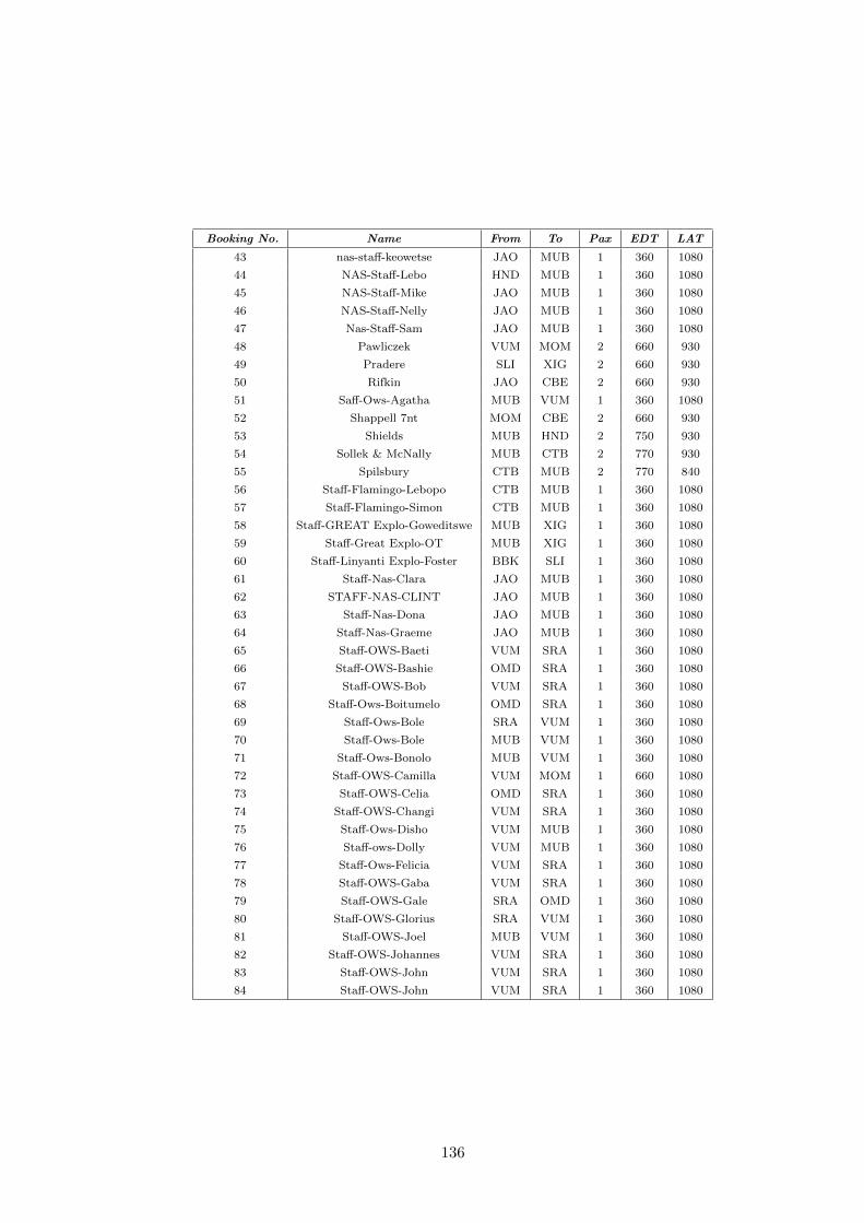
Booking No. Name From To Pax EDT LAT
43 nas-staff-keowetse JAO MUB 1 360 1080
44 NAS-Staff-Lebo HND MUB 1 360 1080
45 NAS-Staff-Mike JAO MUB 1 360 1080
46 NAS-Staff-Nelly JAO MUB 1 360 1080
47 Nas-Staff-Sam JAO MUB 1 360 1080
48 Pawliczek VUM MOM 2 660 930
49 Pradere SLI XIG 2 660 930
50 Rifkin JAO CBE 2 660 930
51 Saff-Ows-Agatha MUB VUM 1 360 1080
52 Shappell 7nt MOM CBE 2 660 930
53 Shields MUB HND 2 750 930
54 Sollek & McNally MUB CTB 2 770 930
55 Spilsbury CTB MUB 2 770 840
56 Staff-Flamingo-Lebopo CTB MUB 1 360 1080
57 Staff-Flamingo-Simon CTB MUB 1 360 1080
58 Staff-GREAT Explo-Goweditswe MUB XIG 1 360 1080
59 Staff-Great Explo-OT MUB XIG 1 360 1080
60 Staff-Linyanti Explo-Foster BBK SLI 1 360 1080
61 Staff-Nas-Clara JAO MUB 1 360 1080
62 STAFF-NAS-CLINT JAO MUB 1 360 1080
63 Staff-Nas-Dona JAO MUB 1 360 1080
64 Staff-Nas-Graeme JAO MUB 1 360 1080
65 Staff-OWS-Baeti VUM SRA 1 360 1080
66 Staff-OWS-Bashie OMD SRA 1 360 1080
67 Staff-OWS-Bob VUM SRA 1 360 1080
68 Staff-Ows-Boitumelo OMD SRA 1 360 1080
69 Staff-Ows-Bole SRA VUM 1 360 1080
70 Staff-Ows-Bole MUB VUM 1 360 1080
71 Staff-Ows-Bonolo MUB VUM 1 360 1080
72 Staff-OWS-Camilla VUM MOM 1 660 1080
73 Staff-OWS-Celia OMD SRA 1 360 1080
74 Staff-OWS-Changi VUM SRA 1 360 1080
75 Staff-Ows-Disho VUM MUB 1 360 1080
76 Staff-ows-Dolly VUM MUB 1 360 1080
77 Staff-Ows-Felicia VUM SRA 1 360 1080
78 Staff-OWS-Gaba VUM SRA 1 360 1080
79 Staff-OWS-Gale SRA OMD 1 360 1080
80 Staff-OWS-Glorius SRA VUM 1 360 1080
81 Staff-OWS-Joel MUB VUM 1 360 1080
82 Staff-OWS-Johannes VUM SRA 1 360 1080
83 Staff-OWS-John VUM SRA 1 360 1080
84 Staff-OWS-John VUM SRA 1 360 1080
136
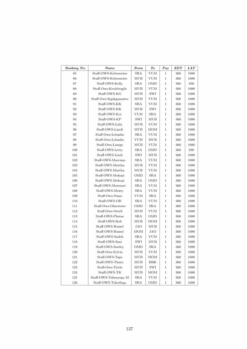
Booking No. Name From To Pax EDT LAT
85 Staff-OWS-Keleemetse SRA VUM 1 360 1080
86 Staff-OWS-Keleemetse MUB VUM 1 360 1080
87 Staff-OWS-Kelly SRA OMD 1 360 930
88 Staff-Ows-Keolebogile MUB VUM 1 360 1080
89 Staff-OWS-KG MUB SWI 1 360 1080
90 Staff-Ows-Kgakgamatso MUB VUM 1 360 1080
91 Staff-OWS-KK SRA VUM 1 360 1080
92 Staff-OWS-KK MUB SWI 1 360 1080
93 Staff-OWS-Koi VUM SRA 1 360 1080
94 Staff-OWS-KP SWI MUB 1 360 1080
95 Staff-OWS-Lalu MUB VUM 1 360 1080
96 Staff-OWS-Landi MUB MOM 1 360 1080
97 Staff-Ows-Lebasho SRA VUM 1 360 1080
98 Staff-Ows-Lebasho VUM MUB 1 360 1080
99 Staff-Ows-Lesego MUB VUM 1 360 1080
100 Staff-OWS-Letty SRA OMD 1 360 930
101 Staff-OWS-Lindi SWI MUB 1 360 1080
102 Staff-OWS-Marriam SRA VUM 1 360 1080
103 Staff-OWS-Martha MUB VUM 1 360 1080
104 Staff-OWS-Martha MUB VUM 1 360 1080
105 Staff-OWS-Mokopi OMD SRA 1 360 1080
106 Staff-OWS-Mokopi SRA OMD 1 360 1080
107 Staff-OWS-Motsumi SRA VUM 1 360 1080
108 Staff-OWS-Motty SRA VUM 1 360 1080
109 Staff-Ows-Nana VUM SRA 1 360 1080
110 Staff-OWS-OB SRA VUM 1 360 1080
111 Staff-Ows-Olatotswe OMD SRA 1 360 1080
112 Staff-Ows-Ortell MUB VUM 1 360 1080
113 Staff-OWS-Phetso SRA OMD 1 360 1080
114 Staff-OWS-Rob MUB MOM 1 360 1080
115 Staff-OWS-Russel JAO MUB 1 360 1080
116 Staff-OWS-Russel MOM JAO 1 360 1080
117 Staff-OWS-Sadek SRA VUM 1 360 1080
118 Staff-OWS-Sam SWI MUB 1 360 1080
119 Staff-OWS-Smiley OMD SRA 1 360 1080
120 Staff-Ows-Sylvia MUB VUM 1 360 1080
121 Staff-OWS-Taps MUB MOM 1 360 1080
122 Staff-OWS-Thuto MUB BBK 1 360 1080
123 Staff-Ows-Tirelo MUB SWI 1 360 1080
124 Staff-OWS-TK MUB MOM 1 360 1080
125 Staff-OWS-Tshenyego M SRA VUM 1 360 1080
126 Staff-OWS-Tshotlego SRA OMD 1 360 1080
137

Booking No. Name From To Pax EDT LAT
127 Staff-Ows-Tshubugo MUB VUM 1 360 1080
128 Staff-Sable-Cathy MUB CBE 1 360 930
129 Staff-Sable-Lee CBE MUB 1 360 1080
130 Staff-Sable-Raymond CBE MUB 1 660 1080
131 Staff-Sable-Rocky MUB CBE 1 360 1080
132 Staff-Sefofane-Lekani BBK MUB 1 360 1080
133 Staff-Sefofane-Modiri CBE MUB 1 360 1080
134 Staff-Sefofane-Ollie MUB VUM 1 360 1080
135 Staff-Sefofane-Tumo BBK MUB 1 360 1080
136 Staff-Sefofane-Witness MUB VUM 1 360 1080
137 Stahl SLI BBK 4 660 930
138 Steel MOM MUB 2 780 840
139 Stewart 7nt VUM CBE 2 660 930
140 Thomas LVI BBK 2 600 865
141 Thomas BBK SLI 2 660 930
142 Thomas & Lorenz CTB JAO 2 660 930
143 Trimble 7nt VUM TSO 2 660 930
144 Word MOM MUB 2 780 840
145 World Jouney Edu/1 HND VUM 4 660 930
146 World Jouneys Edu/2 HND VUM 4 660 930
147 Wright MUB XIG 4 830 930
148 Yoshimoto 7nt CBE BBK 2 660 930
149 Z1-11(08)Guide-Francis XOR XIG 1 660 900
150 Z1-11(08)Macgregor XOR XIG 1 660 900
151 Z1-11(08)McLean XOR XIG 1 660 900
152 Z3-10(08)Guide Richard BBK CBE 1 810 895
153 Z3-10(08)Kauth BBK CBE 2 810 895
154 BOX#67(05/20)2008 MLO VFA 12 815 870
155 BOX#69(05/20)08 VFA MLO 12 735 795
156 BOX#69(08)/1 SWI BBK 12 420 560
157 BOX#71(08)/1 KWD SWI 12 660 900
158 BOX#73(08)/1 BBK KWD 12 600 900
Table A.2: Distance Matrix (kilometres)XOR XIG BBK CBE KWD SWI MUB VUM JAO CTB MOM TSO SRA OMD SHN SLI HND LVI ABU VFA MLO
XOR 0 431 114 284 311 351 391 404 459 373 413 342 429 414 357 312 471 65 457 50 164
XIG 431 0 324 154 154 82 106 44 38 79 22 290 62 48 74 128 49 366 27 382 271
BBK 114 324 0 173 197 247 299 294 349 274 305 301 317 303 250 200 361 52 349 72 81
CBE 284 154 173 0 47 88 164 121 177 125 134 270 145 130 85 28 189 219 178 236 137
KWD 311 154 197 47 0 110 191 113 167 149 132 315 125 117 99 42 177 247 172 266 176
SWI 351 82 247 88 110 0 82 72 116 39 70 234 108 87 18 70 128 286 110 301 189
MUB 391 106 299 164 191 82 0 128 143 44 111 186 161 141 95 151 152 330 128 341 228
VUM 404 44 294 121 113 72 128 0 56 89 23 302 36 15 56 94 68 339 59 355 249
JAO 459 38 349 177 167 116 143 56 0 117 47 328 48 49 105 149 12 394 18 410 302
CTB 373 79 274 125 149 39 44 89 117 0 76 214 124 103 51 109 128 310 105 324 210
MOM 413 22 305 134 132 70 111 23 47 76 0 290 51 32 58 108 59 349 43 364 255
TSO 342 290 301 270 315 234 186 302 328 214 290 0 338 316 252 276 338 302 314 303 222
SRA 429 62 317 145 125 108 161 36 48 124 51 338 0 22 92 117 56 364 62 381 278
OMD 414 48 303 130 117 87 141 15 49 103 32 316 22 0 71 103 60 349 57 366 260
SHN 357 74 250 85 99 18 95 56 105 51 58 252 92 71 0 62 117 292 100 307 197
SLI 312 128 200 28 42 70 151 94 149 109 108 276 117 103 62 0 161 247 151 264 162
HND 471 49 361 189 177 128 152 68 12 128 59 338 56 60 117 161 0 406 24 422 314
LVI 65 366 52 219 247 286 330 339 394 310 349 302 364 349 292 247 406 0 392 20 102
ABU 457 27 349 178 172 110 128 59 18 105 43 314 62 57 100 151 24 392 0 407 298
VFA 50 382 72 236 266 301 341 355 410 324 364 303 381 366 307 264 422 20 407 0 114
MLO 164 271 81 137 176 189 228 249 302 210 255 222 278 260 197 162 314 102 298 114 0
138
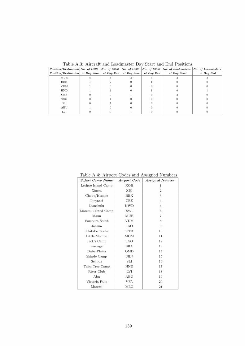
Table A.3: Aircraft and Loadmaster Day Start and End PositionsPosition/Destination No. of C206 No. of C206 No. of C208 No. of C208 No. of Loadmasters No. of Loadmasters
Position/Destination at Day Start at Day End at Day Start at Day End at Day Start at Day End
MUB 5 4 3 3 2 3
BBK 1 2 0 1 0 0
VUM 1 0 0 0 0 0
HND 1 1 0 1 0 1
CBE 0 0 1 0 2 0
TSO 0 1 0 0 0 0
SLI 0 1 0 0 0 0
ABU 1 0 0 0 0 0
LVI 0 0 1 0 0 0
Table A.4: Airport Codes and Assigned NumbersSafari Camp Name Airport Code Assigned Number
Lechwe Island Camp XOR 1
Xigera XIG 2
Chobe/Kasane BBK 3
Linyanti CBE 4
Lianshulu KWD 5
Moremi Tented Camp SWI 6
Maun MUB 7
Vumbura South VUM 8
Jacana JAO 9
Chitabe Trails CTB 10
Little Mombo MOM 11
Jack’s Camp TSO 12
Seronga SRA 13
Duba Plains OMD 14
Shinde Camp SHN 15
Selinda SLI 16
Tubu Tree Camp HND 17
River Club LVI 18
Abu ABU 19
Victoria Falls VFA 20
Matetsi MLO 21
139

APPENDIX B Manual Schedule
140
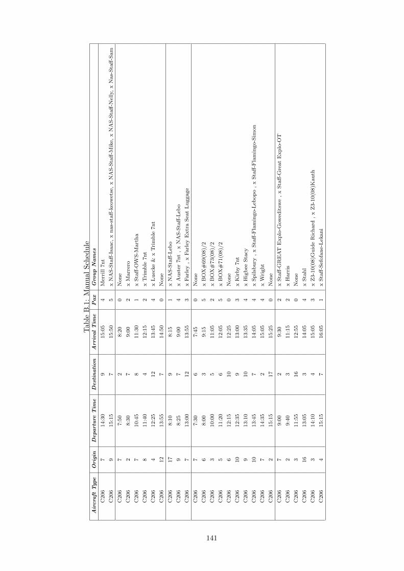
Tab
leB
.1:
Man
ual
Sch
edu
leA
ircra
ftT
ype
Ori
gin
Depart
ure
Tim
eD
est
inati
on
Arr
ival
Tim
eP
ax
Gro
up
Nam
es
C206
714:3
09
15:0
54
Mer
rill
7nt
C206
915:1
57
15:5
05
xN
AS
-Sta
ff-I
saac,
xn
as-
staff
-keo
wet
se,
xN
AS
-Sta
ff-M
ike,
xN
AS
-Sta
ff-N
elly
,x
Nas-
Sta
ff-S
am
C206
77:5
02
8:2
00
Non
e
C206
28:3
07
9:0
02
xM
arr
ero
C206
710:4
58
11:3
01
xS
taff
-OW
S-M
art
ha
C206
811:4
04
12:1
52
xT
rim
ble
7nt
C206
412:2
512
13:4
54
xL
uec
ke
&x
Tri
mb
le7nt
C206
12
13:5
57
14:5
00
Non
e
C206
17
8:1
09
8:1
51
xN
AS
-Sta
ff-L
ebo
C206
98:2
57
9:0
04
xA
ust
er7nt
,x
NA
S-S
taff
-Leb
o
C206
713:0
012
13:5
53
xF
arl
ey,
xF
arl
eyE
xtr
aS
eat
Lu
ggage
C206
77:3
06
7:4
50
Non
e
C206
68:0
03
9:1
55
xB
OX
#69(0
8)/
2
C206
310:0
05
11:0
52
xB
OX
#73(0
8)/
2
C206
511:2
06
12:0
55
xB
OX
#71(0
8)/
2
C206
612:1
510
12:2
50
Non
e
C206
10
12:3
59
13:0
03
xK
irby
7nt
C206
913:1
010
13:3
54
xH
igb
eeS
tacy
C206
10
13:4
57
14:0
54
xS
pilsb
ury
,x
Sta
ff-F
lam
ingo-L
ebop
o,
xS
taff
-Fla
min
go-S
imon
C206
714:3
52
15:0
54
xW
right
C206
215:1
517
15:2
50
Non
e
C206
79:0
02
9:3
02
xS
taff
-GR
EA
TE
xp
lo-G
ow
edit
swe
,x
Sta
ff-G
reat
Exp
lo-O
T
C206
29:4
03
11:1
52
xH
arr
is
C206
311:5
516
12:5
50
Non
e
C206
16
13:0
53
14:0
54
xS
tah
l
C206
314:1
04
15:0
53
xZ
3-1
0(0
8)G
uid
eR
ich
ard
,x
Z3-1
0(0
8)K
au
th
C206
415:1
57
16:0
51
xS
taff
-Sef
ofa
ne-
Lek
an
i
141

Air
cra
ftT
ype
Ori
gin
Depart
ure
Tim
eD
est
inati
on
Arr
ival
Tim
eP
ax
Gro
up
Nam
es
C208
77:4
56
8:0
03
xS
taff
-OW
S-K
G,
xS
taff
-OW
S-K
K,
xS
taff
-Ow
s-T
irel
o
C208
68:2
03
9:1
512
xB
OX
#69(0
8)/
1
C208
310:0
05
10:5
012
xB
OX
#73(0
8)/
1
C208
511:1
06
11:4
512
xB
OX
#71(0
8)/
1
C208
611:5
57
12:1
03
xS
taff
-OW
S-K
P,
xS
taff
-OW
S-L
ind
i,
xS
taff
-OW
S-S
am
C208
713:1
010
13:2
56
xF
reem
an
Kalm
,x
Mahu
lS
hah
,x
Sollek
&M
cNally
C208
10
13:3
59
13:5
55
xH
old
en,
xM
ahu
lS
hah
,x
Th
om
as
&L
ore
nz
C208
914:0
58
14:1
510
xH
old
en,
xM
ahu
lS
hah
,x
NA
S-S
taff
-Joan
ne
,x
Sta
ff-N
as-
Cla
ra,
xS
TA
FF
-NA
S-C
LIN
T,
xS
taff
-Nas-
Don
a,
xS
taff
-Nas-
Gra
eme
,x
Sta
ff-O
WS
-Ru
ssel
C208
814:2
514
14:3
08
xM
ahu
lS
hah
,x
NA
S-S
taff
-Joan
ne
,x
Sta
ff-N
as-
Cla
ra,
xS
TA
FF
-NA
S-C
LIN
T,
xS
taff
-Nas-
Don
a,
xS
taff
-Nas-
Gra
eme
,x
Sta
ff-O
WS
-Ru
ssel
C208
14
14:4
017
14:5
06
xN
AS
-Sta
ff-J
oan
ne
,x
Sta
ff-N
as-
Cla
ra,
xS
TA
FF
-NA
S-C
LIN
T,
xS
taff
-Nas-
Don
a,
xS
taff
-Nas-
Gra
eme
,x
Sta
ff-O
WS
-Ru
ssel
C208
17
15:0
07
15:3
07
xN
AS
-Sta
ff-J
oan
ne
,x
NA
S-S
taff
-Ju
ly,
xS
taff
-Nas-
Cla
ra,
xS
TA
FF
-NA
S-C
LIN
T,
xS
taff
-Nas-
Don
a,
xS
taff
-Nas-
Gra
eme
,x
Sta
ff-O
WS
-Ru
ssel
C208
47:4
07
8:1
56
xB
oeh
mke/
1,
xB
oeh
mke/
2,
xS
taff
-Sab
le-L
ee,
xS
taff
-Sab
le-R
aym
on
d
C208
79:3
019
9:5
50
Non
e
C208
19
10:1
57
10:4
07
xK
esh
avje
eP
art
yS
OL
E208/2
C208
711:2
08
11:5
511
xS
aff
-Ow
s-A
gath
a,
xS
taff
-Ow
s-B
on
olo
,x
Sta
ff-O
WS
-Joe
,x
Sta
ff-O
WS
-Kel
eem
etse
,
xS
taff
-Ow
s-K
eole
bogil
e,x
Sta
ff-O
ws-
Kgakgam
ats
o,
xS
taff
-OW
S-L
alu
,x
Sta
ff-O
ws-
Les
ego,
xS
taff
-Ow
s-O
rtel
,x
Sta
ff-O
ws-
Sylv
ia,
xS
taff
-Ow
s-T
shu
bu
go
C208
812:0
513
12:1
511
xS
taff
-OW
S-B
aet
i,
xS
taff
-OW
S-B
ob
,x
Sta
ff-O
WS
-Ch
an
gi
,x
Sta
ff-O
ws-
Fel
icia
,
xS
taff
-OW
S-G
ab
a,
xS
taff
-OW
S-J
oh
an
nes
,x
Sta
ff-O
WS
-Joh
n,
xS
taff
-OW
S-J
oh
n,
xS
taff
-OW
S-K
elly
,x
Sta
ff-O
WS
-Koi,
xS
taff
-Ow
s-N
an
a
C208
13
12:2
514
12:3
56
xS
taff
-OW
S-G
ale
,x
Sta
ff-O
WS
-Kel
ly,
xS
taff
-OW
S-L
etty
,x
Sta
ff-O
WS
-Mokop
i,
,
xS
taff
-OW
S-P
het
sox
Sta
ff-O
WS
-Tsh
otl
ego
C208
14
12:4
513
12:5
56
xS
taff
-OW
S-B
ash
ie,
xS
taff
-Ow
s-B
oit
um
elo,
xS
taff
-OW
S-C
elia
,x
Sta
ff-O
WS
-Mokop
i,
xS
taff
-Ow
s-O
lato
tsw
e,x
Sta
ff-O
WS
-Sm
iley
C208
13
13:0
58
13:1
511
xS
taff
-Ow
s-B
ole
,x
Sta
ff-O
WS
-Glo
riu
s,
xS
taff
-OW
S-K
elee
met
se,
xS
taff
-OW
S-K
K,
xS
taff
-Ow
s-L
ebash
o,
xS
taff
-OW
S-M
arr
iam
,x
Sta
ff-O
WS
-Mots
um
i,x
Sta
ff-O
WS
-Mott
y,
xS
taff
-OW
S-O
B,
xS
taff
-OW
S-S
ad
ek,
xS
taff
-OW
S-T
shen
yeg
oM
C208
813:2
57
14:0
03
xS
taff
-Ow
s-D
ish
o,
xS
taff
-ow
s-D
olly
,x
Sta
ff-O
ws-
Leb
ash
o
142
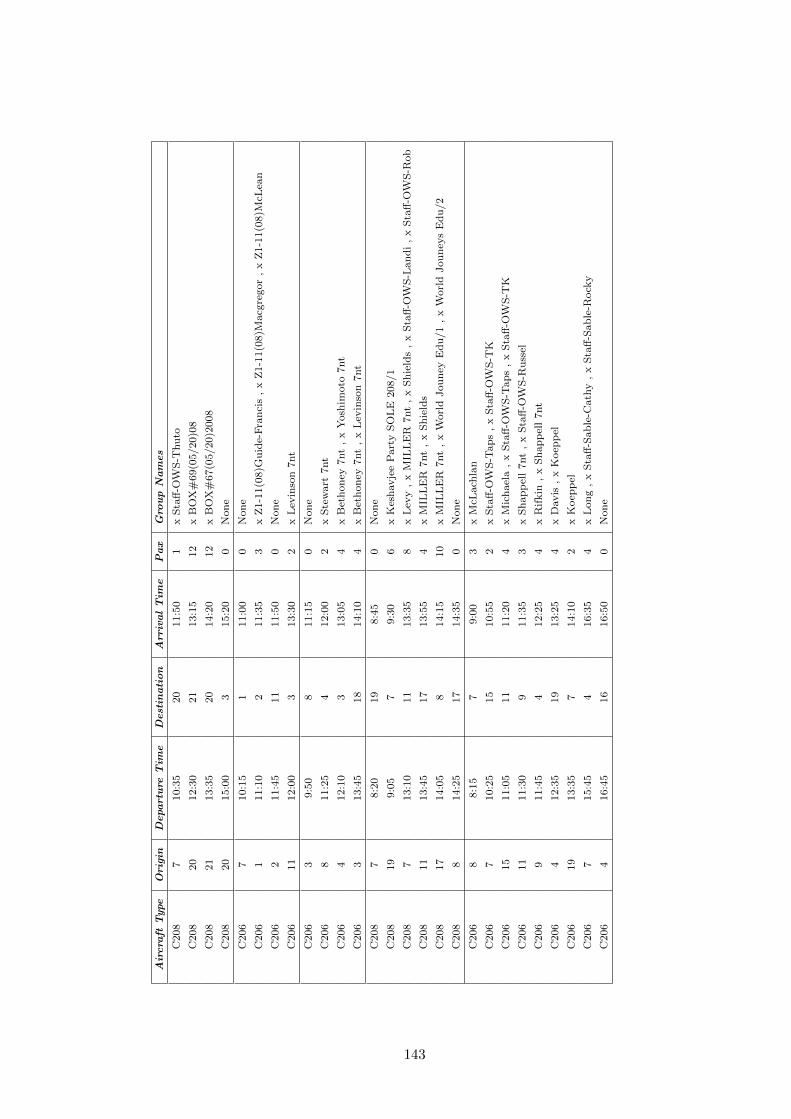
Air
cra
ftT
ype
Ori
gin
Depart
ure
Tim
eD
est
inati
on
Arr
ival
Tim
eP
ax
Gro
up
Nam
es
C208
710:3
520
11:5
01
xS
taff
-OW
S-T
hu
to
C208
20
12:3
021
13:1
512
xB
OX
#69(0
5/20)0
8
C208
21
13:3
520
14:2
012
xB
OX
#67(0
5/20)2
008
C208
20
15:0
03
15:2
00
Non
e
C206
710:1
51
11:0
00
Non
e
C206
111:1
02
11:3
53
xZ
1-1
1(0
8)G
uid
e-F
ran
cis
,x
Z1-1
1(0
8)M
acg
regor
,x
Z1-1
1(0
8)M
cLea
n
C206
211:4
511
11:5
00
Non
e
C206
11
12:0
03
13:3
02
xL
evin
son
7nt
C206
39:5
08
11:1
50
Non
e
C206
811:2
54
12:0
02
xS
tew
art
7nt
C206
412:1
03
13:0
54
xB
eth
on
ey7nt
,x
Yosh
imoto
7nt
C206
313:4
518
14:1
04
xB
eth
on
ey7nt
,x
Lev
inso
n7nt
C208
78:2
019
8:4
50
Non
e
C208
19
9:0
57
9:3
06
xK
esh
avje
eP
art
yS
OL
E208/1
C208
713:1
011
13:3
58
xL
evy
,x
MIL
LE
R7nt
,x
Sh
ield
s,
xS
taff
-OW
S-L
an
di
,x
Sta
ff-O
WS
-Rob
C208
11
13:4
517
13:5
54
xM
ILL
ER
7nt
,x
Sh
ield
s
C208
17
14:0
58
14:1
510
xM
ILL
ER
7nt
,x
Worl
dJou
ney
Ed
u/1
,x
Worl
dJou
ney
sE
du
/2
C208
814:2
517
14:3
50
Non
e
C206
88:1
57
9:0
03
xM
cLach
lan
C206
710:2
515
10:5
52
xS
taff
-OW
S-T
ap
s,
xS
taff
-OW
S-T
K
C206
15
11:0
511
11:2
04
xM
ich
ael
a,
xS
taff
-OW
S-T
ap
s,
xS
taff
-OW
S-T
K
C206
11
11:3
09
11:3
53
xS
hap
pel
l7nt
,x
Sta
ff-O
WS
-Ru
ssel
C206
911:4
54
12:2
54
xR
ifkin
,x
Sh
ap
pel
l7nt
C206
412:3
519
13:2
54
xD
avis
,x
Koep
pel
C206
19
13:3
57
14:1
02
xK
oep
pel
C206
715:4
54
16:3
54
xL
on
g,
xS
taff
-Sab
le-C
ath
y,
xS
taff
-Sab
le-R
ock
y
C206
416:4
516
16:5
00
Non
e
143
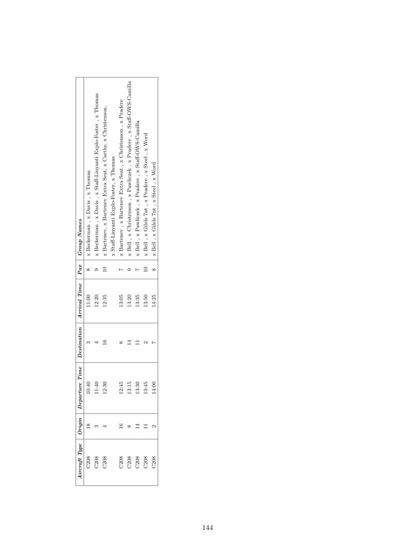
Air
cra
ftT
ype
Ori
gin
Depart
ure
Tim
eD
est
inati
on
Arr
ival
Tim
eP
ax
Gro
up
Nam
es
C208
18
10:4
03
11:0
08
xB
ecker
man
,x
Davis
,x
Th
om
as
C208
311:4
04
12:2
09
xB
ecker
man
,x
Davis
,x
Sta
ff-L
inyanti
Exp
lo-F
ost
er,
xT
hom
as
C208
412:3
016
12:3
510
xB
art
enev
,x
Bart
enev
Extr
aS
eat,
xC
art
hy,
xC
hri
sten
son
,
xS
taff
-Lin
yanti
Exp
lo-F
ost
er,
xT
hom
as
C208
16
12:4
58
13:0
57
xB
art
enev
,x
Bart
enev
Extr
aS
eat
,x
Ch
rist
enso
n,
xP
rad
ere
C208
813:1
514
13:2
09
xB
ell
,x
Ch
rist
enso
n,
xP
aw
licz
ek,
xP
rad
ere
,x
Sta
ff-O
WS
-Cam
illa
C208
14
13:3
011
13:3
57
xB
ell
,x
Paw
licz
ek,
xP
rad
ere
,x
Sta
ff-O
WS
-Cam
illa
C208
11
13:4
52
13:5
010
xB
ell
,x
Gilel
s7nt
,x
Pra
der
e,
xS
teel
,x
Word
C208
214:0
07
14:2
58
xB
ell
,x
Gilel
s7nt
,x
Ste
el,
xW
ord
144
APPENDIX C Aggregation Heuristic Result
145

Table C.1: Aggregated Groups for Full ScheduleAggregated Number of Original Booking
Group No. Passengers List Numbers Booking Names
1 3 1 Auster 7nt
2 3 2, 3 Bartenev, Bartenev Extra Seat
3 4 4 Beckerman1
4 6 5,140 Beckerman2
5 2 6 Bell
6 4 7, 148 Bethoney 7nt1, Yoshimoto 7nt
7 2 8 Bethoney 7nt2
8 4 9, 10 Boehmke/1, Boehmke/2
9 5 11 BOX69(08)/2
10 5 12 BOX71(08)/2
11 2 13 BOX73(08)/2
12 2 14 Carthy
13 2 15 Christenson
14 2 16 Davis
15 2 17 Davis
16 3 18,19 Farley, Farley Extra Seat Luggage
17 4 20,54 Freeman Kalm, Sollek, McNally
18 6 21,138,21,144 Gilels 7nt, Steel, Word
19 2 22 Harris
20 4 23 Higbee Stacy
21 2 24 Holden
22 6 25 Keshavjee Party SOLE 208/1
23 7 26 Keshavjee Party SOLE 208/2
24 5 27,142 Kirby 7ntm Thomas, Lorenz
25 2 28 Koeppel
26 2 29 Levinson 7nt
27 2 30 Levinson 7nt
28 2 31 Levy
29 2 32 Long
30 2 33 Luecke
31 2 34 Mahul Shah
32 2 35 Marrero
33 3 36 McLachlan
34 4 37 Merrill 7nt
35 2 38 Michaela
36 2 39 MILLER 7nt
37 11 40,41,40,43,40, NAS-Staff-Isaac, NAS-Staff-Joanne, nas-staff-keowetse,
45,40,46,40,47, NAS-Staff-Mike, NAS-Staff-Nelly, Nas-Staff-Sam,
40,61,40,62,40, Staff-Nas-Clara, STAFF-NAS-CLINT, Staff-Nas-Dona,
63,40,64,40,115 Staff-Nas-Graeme, Staff-OWS-Russel
38 2 42,44 NAS-Staff-July, NAS-Staff-Lebo
39 2 48 Pawliczek
40 2 49 Pradere
41 2 50 Rifkin
42 11 51,70,51,71,51, Saff-Ows-Agatha, Staff-Ows-Bole, Staff-Ows-Bonolo,
81,51,86,51,88, Staff-OWS-Joel, Staff-OWS-Keleemetse, Staff-Ows-Keolebogile ,
51,90,51,95,51, Staff-Ows-Kgakgamatso, Staff-OWS-Lalu,Staff-Ows-Lesego,
99,51,103,51,104 Staff-OWS-Martha, Staff-OWS-Martha
43 2 52 Shappell 7nt
44 2 53 Shields
146

Aggregated Number of Original Booking
Group No. Passengers List Numbers Booking Names
45 2 55 Spilsbury
46 2 56,57 Staff-Flamingo-Lebopo, Staff-Flamingo-Simon
47 2 58,59 Staff-GREAT Explo-Goweditswe, Staff-Great Explo-OT
48 1 60 Staff-Linyanti Explo-Foster
49 10 65,67,65,74,65, Staff-OWS-Baeti, Staff-OWS-Bob, Staff-OWS-Changi,
77,65,78,65,82, Staff-Ows-Felicia, Staff-OWS-Gaba, Staff-OWS-Johannes,
65,83,65,84,65, Staff-OWS-John, Staff-OWS-John, Staff-OWS-Koi,
93,65,109 Staff-Ows-Nana
50 6 66,68,66,73,66, Staff-OWS-Bashie, Staff-Ows-Boitumelo, Staff-OWS-Celia,
105,66,111,66,119 Staff-OWS-Mokopi, Staff-Ows-Olatotswe, Staff-OWS-Smiley
51 11 69,80,69,85,69, Staff-Ows-Bole, Staff-OWS-Glorius, Staff-OWS-Keleemetse,
91,69,97,69,102, Staff-OWS-KK, Staff-Ows-Lebasho, Staff-OWS-Marriam,
69,107,69,108,69, Staff-OWS-Motsumi, Staff-OWS-Motty, Staff-OWS-OB,
110,69,117,69,125 Staff-OWS-Sadek, Staff-OWS-Tshenyego M
52 1 72 Staff-OWS-Camilla
53 3 75,76,75,98 Staff-Ows-Disho, Staff-ows-Dolly, Staff-Ows-Lebasho
54 4 79,106,79,113,79, Staff-OWS-Gale, Staff-OWS-Mokopi, Staff-OWS-Phetso,
126 Staff-OWS-Tshotlego
55 2 87,100 Staff-OWS-Kelly, Staff-OWS-Letty
56 3 89,92,89,123 Staff-OWS-KG, Staff-OWS-KK, Staff-Ows-Tirelo
57 3 94,101,94,118 Staff-OWS-KP, Staff-OWS-Lindi, Staff-OWS-Sam
58 4 96,114,96,121,96, Staff-OWS-Landi, Staff-OWS-Rob, Staff-OWS-Taps,
124 Staff-OWS-TK
59 5 112,120,112,127,112, Staff-Ows-Ortell, Staff-Ows-Sylvia, Staff-Ows-Tshubugo,
134,112,136 Staff-Sefofane-Ollie, Staff-Sefofane-Witness
60 1 116 Staff-OWS-Russel
61 1 122 Staff-OWS-Thuto
62 1 128 Staff-Sable-Cathy
63 2 129,133 ,129,133
64 1 130 Staff-Sable-Raymond
65 1 131 Staff-Sable-Rocky
66 2 132,135 Staff-Sefofane-Lekani, Staff-Sefofane-Tumo
67 4 137 Stahl
68 2 139 Stewart 7nt
69 2 141 Thomas
70 2 143 Trimble 7nt
71 8 145,146 World Jouney Edu/1, World Jouneys Edu/2
72 4 147 Wright
73 3 149,150,149,151 Z1-11(08)Guide-Francis, Z1-11(08)Macgregor, Z1-11(08)McLean
74 3 152,153 Z3-10(08)Guide Richard, Z3-10(08)Kauth
75 12 154 BOX67(05/20)2008
76 12 155 BOX69(05/20)08
77 12 156 BOX69(08)/1
78 12 157 BOX71(08)/1
79 12 158 BOX73(08)/1
147

APPENDIX D Agent Routing MATLAB
Code - Airline Taxi Problem
D.1 Attractiveness Parameters
Fac1(1,1)=30; % time urgency factor 1
Fac1(2,1)=4; % number of on board groups with destinations matching candidate location
Fac1(3,1)=30; % time closeness
Fac1(4,1)=50; % geographic closeness
Fac1(5,1)=4; % on-board group destinations match awaiting group destinations
Fac1(6,1)=0.5; % if subsequent collected groups have the same destination as previously collected groups from same location (selection of groups to collect)
Fac1(7,1)=15; % take off and leave any other waiting groups (selection of groups to collect)
Fac1(8,1)=20; % time urgency factor 2 - for on-board groups
Fac1(9,1)=1/20; % awaiting group size
D.2 Agent Routing Function
function [f u]=Fn_Agent_Fixed_V2(Fac1)
%Fac1 is a vector of attractiveness factors
global sch
global fleet
global fleetType
global dest
Fix1=1; % make best decisions only
NIters=1;
Penalty=10000; %cost for every undelivered item
Fac1=Fac1’;
u=0;
148
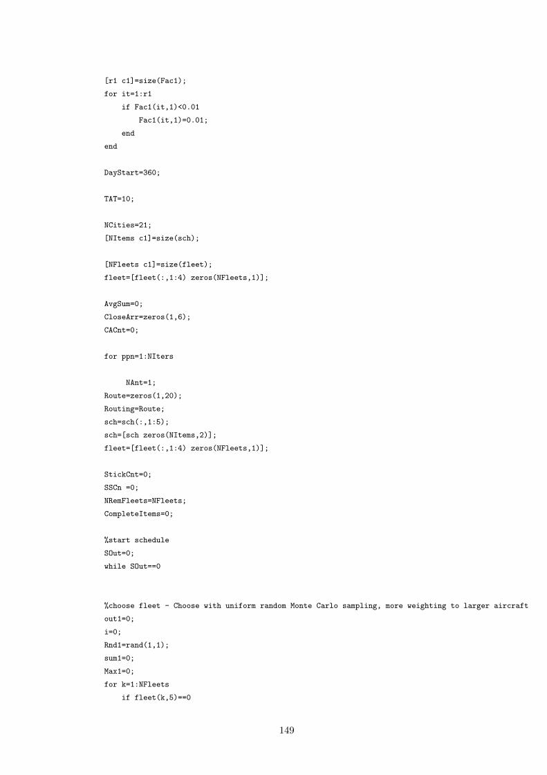
[r1 c1]=size(Fac1);
for it=1:r1
if Fac1(it,1)<0.01
Fac1(it,1)=0.01;
end
end
DayStart=360;
TAT=10;
NCities=21;
[NItems c1]=size(sch);
[NFleets c1]=size(fleet);
fleet=[fleet(:,1:4) zeros(NFleets,1)];
AvgSum=0;
CloseArr=zeros(1,6);
CACnt=0;
for ppn=1:NIters
NAnt=1;
Route=zeros(1,20);
Routing=Route;
sch=sch(:,1:5);
sch=[sch zeros(NItems,2)];
fleet=[fleet(:,1:4) zeros(NFleets,1)];
StickCnt=0;
SSCn =0;
NRemFleets=NFleets;
CompleteItems=0;
%start schedule
SOut=0;
while SOut==0
%choose fleet - Choose with uniform random Monte Carlo sampling, more weighting to larger aircraft
out1=0;
i=0;
Rnd1=rand(1,1);
sum1=0;
Max1=0;
for k=1:NFleets
if fleet(k,5)==0
149

sum1=sum1+fleetType(fleet(k,2),3);
if fleetType(fleet(k,2),3)>Max1
Max1=fleetType(fleet(k,2),3);
end
end
end
cum1=0;
while out1==0
i=i+1;
if fleet(i,5)==0
if Fix1==0
cum1=cum1+fleetType(fleet(i,2),3)*(1-fleet(i,5));
if Rnd1<=cum1/sum1
out1=1;
end
else
if Max1==fleetType(fleet(i,2),3)
out1=1;
end
end
end
end
ant(1,1)=i;
Flt1=i;
NRemFleets=NRemFleets-1;
fleet(i,5)=1;
CurrCity=fleet(ant(1,1),3);
CurrTime=DayStart;
FltSpd=fleetType(fleet(ant(1,1),2),2);
EmptySeats=fleetType(fleet(ant(1,1),2),3);
NOnBrd=0;
OnBrd=[];
%record route
Route(1,1)=CurrCity;
Route(1,2)=DayStart;
Route(1,3)=EmptySeats;
Route(1,5)=NOnBrd;
Route(1,4)=Flt1;
for pp=1:NOnBrd
150

Route(1,5+pp)=OnBrd(pp,6);
end
%step ant through day
NOut=0;
StepCnt=1;
while NOut==0
%choose next destination
Att=zeros(NCities,2);
Choose1=zeros(NCities,1);
ArrivalTime=Choose1;
CanPick=zeros(NCities,50); % grp number is j,1
CanPickAttr=CanPick;
MustGo=zeros(NCities,1);
for j=1:NCities
%Attractiveness:
%distance
Dist1=distance2(dest,CurrCity,j);
FlTime=Dist1/FltSpd*60;
ArrivalTime(j,1)=CurrTime+FlTime;
% Geographic closeness
Close3= 1 / exp(Dist1 / Fac1(4,1));
%On-board grps
ReasonFlag=0;
NOnBrdDests=0;
TimeClose=0;
for i=1:NOnBrd
if OnBrd(i,4)==j
ReasonFlag=1;
Att(j,1)=1;
NOnBrdDests=NOnBrdDests+1;
%how soon must they arrive at dest?
t1=ArrivalTime(j,1);
t2=OnBrd(i,2);
TU=1 / exp((abs(t2 - t1) / Fac1(1,1)));
% TU=TimeUrgency(Sch(OnBrd(i,1),2),ArrivalTime(j,1);
TimeClose=TimeClose+TU;
if (t2-t1)<TU*Fac1(8,1)
MustGo(j,1)=1;
end
end
151
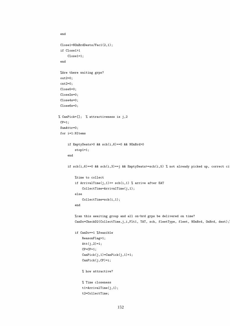
end
Close1=NOnBrdDests/Fac1(2,1);
if Close1>1
Close1=1;
end
%Are there waiting grps?
out2=0;
cnt2=0;
Close5=0;
Close2s=0;
Close4s=0;
Close6s=0;
% CanPick=[]; % attractiveness is j,2
CP=1;
SumAttr=0;
for i=1:NItems
if EmptySeats>0 && sch(i,6)==0 && NOnBrd>0
stop1=1;
end
if sch(i,6)==0 && sch(i,3)==j && EmptySeats>=sch(i,5) % not already picked up, correct city, enough space
%time to collect
if ArrivalTime(j,1)>= sch(i,1) % arrive after EAT
CollectTime=ArrivalTime(j,1);
else
CollectTime=sch(i,1);
end
%can this awaiting group and all on-brd grps be delivered on time?
CanDo=CheckD2(CollectTime,j,i,Flt1, TAT, sch, fleetType, fleet, NOnBrd, OnBrd, dest);%TimeToCollect, CollectionCity, GrpToCollect, fleet, TATime
if CanDo==1 %feasible
ReasonFlag=1;
Att(j,2)=1;
CP=CP+1;
CanPick(j,1)=CanPick(j,1)+1;
CanPick(j,CP)=i;
% how attractive?
% Time closeness
t1=ArrivalTime(j,1);
t2=CollectTime;
152
TU=1 / exp((abs(t2 - t1) / Fac1(3,1)));
Close2=TU;
% dest. of waiting grp = on brd grp destinations
OBDMatchCnt=0;
cnt9=0;
out9=0;
for k=1:NOnBrd
if OnBrd(k,4)==sch(i,4)
OBDMatchCnt=OBDMatchCnt+1;
end
end
Close4=OBDMatchCnt/Fac1(5,1);
if Close4>1
Close4=1;
end
%size - make larger groups more attractive
Close6=sch(i,5)*Fac1(9,1);
xx=Close2+Close4+Close6;
Close5=Close5+xx;
CanPickAttr(j,CP)=xx;
SumAttr=SumAttr+xx;
Close2s=Close2s+Close2;
Close4s=Close4s+Close4;
Close6s=Close6s+Close6;
end
end
end
if ReasonFlag==1
Choose1(j,1)=Close1+Close3+Close5+TimeClose;
else
Choose1(j,1)=0;
end
CACnt=CACnt+1;
CloseArr(CACnt,1)=Close1;
CloseArr(CACnt,2)=Close3;
CloseArr(CACnt,3)=TimeClose;
CloseArr(CACnt,4)=Close2s;
CloseArr(CACnt,5)=Close4s;
CloseArr(CACnt,6)=Close6s;
CloseArr(CACnt,7)=Close5;
153

end
%if urgent matter:
Filter11=0;
for j=1:NCities
if MustGo(j,1)==1
NextCity=j;
Filter11=1;
end
end
%Filter11;
if Filter11==0
AllZeros=1;
for k=1:NCities
if Choose1(k,1)>0.01
AllZeros=0;
end
end
end
if AllZeros==0
%Monte Carlo - sample next city to go to
Rnd1=rand(1,1);
sum1=0;
Max1=0;
for j=1:NCities
sum1=sum1+Choose1(j,1);
if Choose1(j,1)>Max1
Max1=Choose1(j,1);
end
end
out2=0;
cnt2=0;
cum2=0;
while out2==0
cnt2=cnt2+1;
if Fix1==0
cum2=cum2+Choose1(cnt2,1);
if Rnd1<=cum2/sum1
NextCity=cnt2;
154

out2=1;
%cnt2=cnt2+1;
if cnt2>NCities
out2=1;
end
end
else
if Choose1(cnt2,1)==Max1
NextCity=cnt2;
out2=1;
end
end
end
end
if AllZeros==0 || Filter11==1 %there is somewhere to go
%move to next city
StepCnt=StepCnt+1;
%record route
Route(StepCnt,1)=NextCity;
Route(StepCnt,2)=ArrivalTime(NextCity,1);
Route(StepCnt,3)=EmptySeats;
Route(StepCnt,5)=NOnBrd;
Route(StepCnt,4)=Flt1;
for pp=1:NOnBrd
Route(StepCnt,5+pp)=OnBrd(pp,6);
end
if CurrCity~=NextCity
CurrTime=ArrivalTime(NextCity,1)+TAT;
end
CurrCity=NextCity;
%are grps dropped off?
Dropped=0;
if Att(CurrCity,1)==1 %yes
Dropped=1;
DelCnt=0;
for i=1:NOnBrd
if OnBrd(i,4)==CurrCity
%remove group
DelCnt=DelCnt+1;
DelGrp=OnBrd(i,6);
DelItem(DelCnt,1)=i;
sch(DelGrp,7)=1;
155
end
end
for ij=1:DelCnt
OnBrd(DelItem(ij,1),8)=1;
%update schedule
%update empty seats
EmptySeats=EmptySeats+sch(DelGrp,5);
end
Dum1=[];
cnt111=0;
for ij=1:NOnBrd
if OnBrd(ij,8)==0
cnt111=cnt111+1;
Dum1(cnt111,:)=OnBrd(ij,:);
end
end
OnBrd=Dum1;
NOnBrd=NOnBrd-DelCnt;
CompleteItems=CompleteItems+DelCnt;
end
%are grps picked up?
TOAttr=0;
if Att(CurrCity,2)==1 % yes
%randomly select grps to collect from CanPick list until plane
%is full
%then move time forward till then
TimeL=zeros(11,1);
AddG=0;
AttrBoost=zeros(NCities,1);
TList=[];
GList=[];
out6=0;
while out6==0
NPick=CanPick(CurrCity,1);
%boost attr for same destinations of grps put on previously
for g=1:NPick
for k=1:NItems
if CanPick(CurrCity,g+1)==k
if k==sch(CanPick(CurrCity,g+1),4)
CanPickAttr(CurrCity,1+g)=CanPickAttr(CurrCity,1+g)+AttrBoost(k,1)*Fac1(6,1);
156

AttrBoost(k,1)=0;
end
%remove attractiveness of grps that can’t fit
if sch(CanPick(CurrCity,g+1),5)>EmptySeats
CanPickAttr(CurrCity,1+g)=0;
end
end
end
end
%add attractiveness to just take off - only if grps were
%dropped off
if Dropped==1
%min waiting time for grps to collect
Nt1=CurrTime;
if AddG>0
for k=1:AddG
if TList(k,1)>Nt1
Nt1=TList(k,1);
end
end
end
MinTOTime=2000;
for g=1:NPick
if sch(CanPick(CurrCity,g+1),1)<MinTOTime
MinTOTime=sch(CanPick(CurrCity,g+1),1);
end
end
TWait=MinTOTime-Nt1;
if TWait<0
TWait=0;
end
TOAttr=1-1/exp(TWait/Fac1(7,1));
if TOAttr<=0.01
TOAttr=0.01;
end
end
Max1=0;
sum1=0; %Monte Carlo sample waiting grps
for g=1:NPick
sum1=sum1+CanPickAttr(CurrCity,1+g);
if CanPickAttr(CurrCity,1+g)>Max1
Max1=CanPickAttr(CurrCity,1+g);
end
end
157

% if sum1<0.01
% TOAttr=1;
% end
if sum1>0.01 %there are grps to collect that can fit
sum1=sum1+TOAttr;
SSCn=SSCn+1;
if SSCn>500
stop1=1;
end
out8=0;
cnt8=0;
cum1=0;
Rnd1=rand(1,1);
while out8==0
cnt8=cnt8+1;
if Fix1==0
if cnt8<=NPick
cum1=cum1+CanPickAttr(CurrCity,cnt8+1);
else
cum1=cum1+TOAttr;
out8=1;
end
if Rnd1<=cum1/sum1
out8=1;
end
else
if Max1==CanPickAttr(CurrCity,1+cnt8)
out8=1;
end
end
end
if cnt8<=NPick %going to pick up a group
PGrp=CanPick(CurrCity,cnt8+1);
%check that dupl grp not being put on brd
find1=0;
for i=1:NOnBrd
if PGrp==OnBrd(i,6)
find1=1;
%***
158

%remove grp from CanPick list
CanPick(CurrCity,1)=CanPick(CurrCity,1)-1;
NPick=CanPick(CurrCity,1);
out8=0;
cnt8=1;
while out8==0
cnt8=cnt8+1;
if CanPick(CurrCity,cnt8)==PGrp
CanPick(CurrCity, cnt8)=0;
for i=cnt8:NPick+1
CanPick(CurrCity,i)=CanPick(CurrCity,i+1);
CanPickAttr(CurrCity,i)=CanPickAttr(CurrCity,i+1);
end
out8=1;
end
end
CanPick(CurrCity,i+1)=0;
CanPickAttr(CurrCity,i+1)=0;
NPick=CanPick(CurrCity,1);
%***
end
end
%check that all grps can still be delivered on time
TimeToCollect=sch(PGrp,1);
CanDo=CheckD2(TimeToCollect, CurrCity, PGrp, Flt1, TAT,sch,fleetType,fleet,NOnBrd,OnBrd,dest);
%TToCollect, City1, GrpToGo, flt1, TATime, sch1, fleetType1, fleet1, NOnBrd1, OnBrd1, dest1
if CanDo==0
find1=1;
%remove grp from CanPick list
CanPick(CurrCity,1)=CanPick(CurrCity,1)-1;
NPick=CanPick(CurrCity,1);
out8=0;
cnt8=1;
while out8==0
cnt8=cnt8+1;
if cnt8>30
stop1=1;
end
if CanPick(CurrCity,cnt8)==PGrp
CanPick(CurrCity, cnt8)=0;
for i=cnt8:NPick+2
CanPick(CurrCity,i)=CanPick(CurrCity,i+1);
159
CanPickAttr(CurrCity,i)=CanPickAttr(CurrCity,i+1);
end
out8=1;
end
end
NPick=CanPick(CurrCity,1);
end
if find1==0 % put grp on board
EmptySeats=EmptySeats-sch(PGrp,5);
NOnBrd=NOnBrd+1;
OnBrd=[OnBrd; sch(PGrp,1:5) PGrp 0 0];
sch(PGrp,6)=1;
AddG=AddG+1;
TList(AddG,1)=sch(PGrp,1); % save EDT
GList(AddG,1)=PGrp;
%boost attractiveness for grps going to same dest as this
%one:
AttrBoost(sch(PGrp,4),1)=AttrBoost(sch(PGrp,4),1)+1;
%remove grp from CanPick list
CanPick(CurrCity,1)=CanPick(CurrCity,1)-1;
NPick=CanPick(CurrCity,1);
out8=0;
cnt8=1;
while out8==0
cnt8=cnt8+1;
if CanPick(CurrCity,cnt8)==PGrp
CanPick(CurrCity, cnt8)=0;
for i=cnt8:NPick+1
CanPick(CurrCity,i)=CanPick(CurrCity,i+1);
CanPickAttr(CurrCity,i)=CanPickAttr(CurrCity,i+1);
end
out8=1;
end
end
CanPick(CurrCity,i+1)=0;
CanPickAttr(CurrCity,i+1)=0;
NPick=CanPick(CurrCity,1);
%add attractiveness to just take off
Dropped=1;
end %putting grp on brd
160

else
%have selected to just take off
out6=1;
end
else %no more grps to take on brd
out6=1;
end
end
%move time forward
TOTime=CurrTime;
for k=1:AddG
if sch(GList(AddG,1),1)>TOTime
TOTime=sch(GList(AddG,1),1);
end
end
CurrTime=TOTime;
end %picking up grps
StepCnt=StepCnt+1;
Route(StepCnt,3)=EmptySeats;
Route(StepCnt,1)=CurrCity;
Route(StepCnt,2)=CurrTime;
Route(StepCnt,5)=NOnBrd;
Route(StepCnt,4)=Flt1;
for pp=1:NOnBrd
Route(StepCnt,5+pp)=OnBrd(pp,6);
end
else
%nowhere to go - all cities zero attractiveness
%new ant
NOut=1;
[r1 c1]=size(Routing);
[r2 c2]=size(Route);
cntn=0;
for kj=r1+1:r1+r2
cntn=cntn+1;
Routing(kj,:)=Route(cntn,:);
end
Route=zeros(1,20);
NAnt=NAnt+1;
%check if schedule is complete
if CompleteItems>=NItems
161

SOut=1;
end
%any remaining agents/planes?
if NRemFleets<=0 %No - finish off
SOut=1;
end
end % end - there is nowhere to go
StickCnt=StickCnt+1;
if StickCnt>1000
stop1=1;
end
end %while NOut - ant out
% set new ant and new time
CurrTime=DayStart;
%SOut=1; %schedule complete
end %schedule complete - SOut
%calculate route cost
[r1 c1]=size(Routing);
TotCost=0;
for i=2:r1
Flt1=Routing(i,4);
NOnBrd=Routing(i,5);
Des1=Routing(i,1);
Tim1=Routing(i,2);
EmptyS=Routing(i,3);
FltCost=fleetType(fleet(Flt1,2),4);
if i>2
Or1=Routing(i-1,1);
TimO=Routing(i-1,2);
if Des1~=Or1
if Tim1>TimO
FlTime=Tim1-TimO;
162
Cost1=FltCost*FlTime/60;
if Cost1<0
stop1=1;
end
TotCost=TotCost+Cost1;
end
end
end
end
%xlswrite(’routing.xlsx’,Routing);
TotCost;
Penal=(NItems-CompleteItems)*Penalty;
TotCost=TotCost+Penal;
u=u+NItems-CompleteItems;
CompleteItems;
AvgSum=AvgSum+TotCost;
end
f=AvgSum/NIters;
%xlswrite(’CloseArr.xlsx’,CloseArr);
end
function z=CheckD2(TToCollect, City1, GrpToGo, flt1, TATime, sch1, fleetType1, fleet1, NOnBrd1, OnBrd1, dest1)
%function to check whether feasibility can be maintained if a certain city is visited
%city1, TTCollect =where we currently are in space-time
GrpNo=GrpToGo;
Time1=TToCollect;
NDests=2;
DestList=[City1 Time1 0]; %dest. city, time to collect (current time)
DestList=[DestList; sch1(GrpNo,4) sch1(GrpNo,2) 0] ; % grp dest , LAT
fltSpd=fleetType1(fleet1(flt1,2),2);
if NOnBrd1>0
for p=1:NOnBrd1
NotIn=0;
for q=1:NDests
%is dest already in dest list?
163

if OnBrd1(p,4)==DestList(q,1)
NotIn=1; %dest. already on list
if OnBrd1(p,2)<DestList(q,2)
DestList(q,2)=OnBrd1(p,2);
end
end
end
if NotIn==0
%add dest to list
NDests=NDests+1;
DestList=[DestList; OnBrd1(p,4) OnBrd1(p,2) 0];
end
end
end
%Travel times table
TTable=zeros(NDests,NDests);
for p=1:NDests
for q=1:NDests
dist1=distance2(dest1,DestList(p,1),DestList(q,1));
flTime=dist1/fltSpd*60;
TTable(DestList(p,1),DestList(q,1))=flTime;
TTable(DestList(q,1),DestList(p,1))=flTime;
end
end
%feasible route search
feasible=1;
outt1=0;
cntt1=2;
CCity=City1;
CTime=Time1;
Ind1=2;
oldCnt(Ind1,1)=1;
DestList(1,3)=1;
StrtPt=zeros(NDests,1);
for i=1:2
StrtPt(i,1)=i;
%DestList(i,3)=0;
end
IndexM=zeros(NDests,2); %prev node index and time
IndexM(1,1)=1;
IndexM(1,2)=CTime;
IndexM(1,3)=CCity;
RowInd=StrtPt;
ReOrder=1;
164
OrigPt=StrtPt;
while outt1==0
if ReOrder==1
%reorder lower levels and strtPts
StrtPt=RowInd;
for kk=Ind1+1:NDests
outp=0;
while outp==0
StrtPt(kk,1)= StrtPt(kk,1)+1;
if StrtPt(kk,1)>NDests
StrtPt(kk,1)=1;
end
OrigPt(kk,1)=StrtPt(kk,1);
fnd1=0;
for kkk=1:kk-1
if StrtPt(kk,1)==RowInd(kkk,1)
fnd1=1;
end
end
if fnd1==0
outp=1;
RowInd(kk,1)=StrtPt(kk,1);
end
end
end
ReOrder=0;
end
if DestList(RowInd(Ind1,1), 1) ~= CCity && DestList(RowInd(Ind1,1), 3) ~= 1 % not curr city AND haven’t already been there
NCity = DestList(RowInd(Ind1,1), 1);
NTime = CTime + TTable(CCity, NCity);
DestList(RowInd(Ind1,1), 3) = 1;
IndexM(Ind1,1)=RowInd(cntt1,1);
IndexM(Ind1,2)=NTime;
IndexM(Ind1,3)=NCity;
if NTime > DestList(RowInd(Ind1,1), 2)
%infeasible
%move sideways
165

DestList(RowInd(Ind1,1), 3) = 0;
Back1=1;
while Back1==1
outp=0;
while outp==0
RowInd(Ind1,1)=RowInd(Ind1,1)+1;
if RowInd(Ind1,1)>NDests
RowInd(Ind1,1)=1;
end
fnd1=0;
for ii=1:Ind1-1
if RowInd(ii,1)==RowInd(Ind1,1)
fnd1=1;
end
end
if fnd1==0
outp=1;
end
%check if RowInd has gone all the way - from StrtPt to
%StrtPt - if yes, move up a level and reset StrtPt.
if RowInd(Ind1,1)==OrigPt(Ind1,1)
Back1=1;
else
Back1=0;
end
ReOrder=1;
end
%else
%5- backtrack to previous level
% DestList(RowInd(Ind1,1), 3) = 0;
%change previous level city
if Back1==1
Ind1 = Ind1 - 1;
DestList(RowInd(Ind1,1), 3) = 0;
First1=0;
if Ind1>2
CTime = IndexM(Ind1-1,2)+TATime;
else
if Ind1~=1
166
CTime=IndexM(Ind1-1,2);
else
CTime=IndexM(Ind1,2);
First1=1;
outt1=1;
feasible=0;
Back1=0;
end
end
if outt1==0
if Ind1~=1
CCity=IndexM(Ind1-1,3);
else
CCity=IndexM(Ind1,3);
end
end
if outt1==0
%DestList(RowInd(Ind1,1), 3) = 0;
outp=0;
OutCnt=0;
while outp==0
OutCnt=OutCnt+1;
RowInd(Ind1,1)=RowInd(Ind1,1)+1;
if RowInd(Ind1,1)>NDests
RowInd(Ind1,1)=1;
end
fnd1=0;
for ii=1:Ind1-1
if RowInd(ii,1)==RowInd(Ind1,1)
fnd1=1;
end
end
if fnd1==0 || OutCnt>NDests
outp=1;
end
%check if RowInd has gone all the way - from StrtPt to
%StrtPt - if yes, move up a level and reset StrtPt.
if RowInd(Ind1,1)==OrigPt(Ind1,1)
Back1=1;
Ind1=Ind1-1;
DestList(RowInd(Ind1,1), 3) = 0;
167
if First1==1
outt1=1;
end
else
Back1=0;
end
end
ReOrder=1;
end
end
end
else %move on
CTime = NTime + TATime;
CCity = NCity;
Ind1 = Ind1 + 1;
oldCnt(Ind1, 1) = 0;
cntt1 = 1;
end
else
cntt1 = cntt1 + 1;
if cntt1>6
outt1=1;
end
end
ROu=1;
for tt = 1:NDests
if DestList(tt, 3) <= 0.1
ROu = 0;
end
end
if ROu==1
outt1=1;
end
z = feasible; %0 no feasible route, 1 feasible
end
end
168
APPENDIX E Agent-Generated Variable
Schedule
169
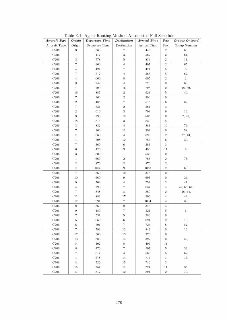
Table E.1: Agent Routing Method Automated Full ScheduleAircraft Type Origin Departure Time Destination Arrival Time Pax Groups Onboard
Aircraft Type Origin Departure Time Destination Arrival Time Pax Group Numbers
C206 3 360 7 445 2 66,
C206 7 477 3 562 2 61,
C206 3 778 5 834 2 11,
C206 7 360 4 407 2 65,
C206 4 424 7 471 5 8,
C206 7 517 4 563 5 62,
C206 4 660 8 695 2 2,
C206 8 742 4 776 0 68,
C206 4 790 16 798 0 48, 69,
C206 16 887 2 923 5 40,
C206 7 360 2 390 0
C206 2 485 7 515 6 32,
C206 7 531 2 561 3
C206 2 610 3 703 9 19,
C206 3 790 18 805 0 7, 26,
C206 18 815 3 830 5
C206 3 832 4 881 10 74,
C206 7 360 11 392 0 58,
C206 11 660 4 698 2 27, 43,
C206 4 708 12 785 6 30,
C206 7 360 6 383 3
C206 6 420 3 490 11 9,
C206 3 500 1 533 0
C206 1 660 2 783 2 73,
C206 2 870 11 876 2
C206 11 1039 9 1053 2 60,
C206 7 360 10 373 0
C206 10 660 9 693 0 24,
C206 9 703 4 754 2 41,
C206 4 790 7 837 4 25, 63, 64,
C206 7 848 11 880 2 28, 44,
C206 11 883 17 900 4 44,
C206 17 991 7 1034 4 38,
C206 8 360 9 376 4
C206 9 480 7 521 5 1,
C206 7 531 5 586 0
C206 5 660 6 691 2 10,
C206 6 701 7 725 8 57,
C206 7 793 12 843 0 16,
C206 17 360 13 376 0
C206 13 386 14 392 0 55,
C206 14 402 8 406 11
C206 8 470 7 507 5 33,
C206 7 517 4 563 5 62,
C206 4 678 14 715 1 13,
C206 14 720 15 740 2
C206 15 757 11 774 11 35,
C206 11 812 12 894 2 70,
170
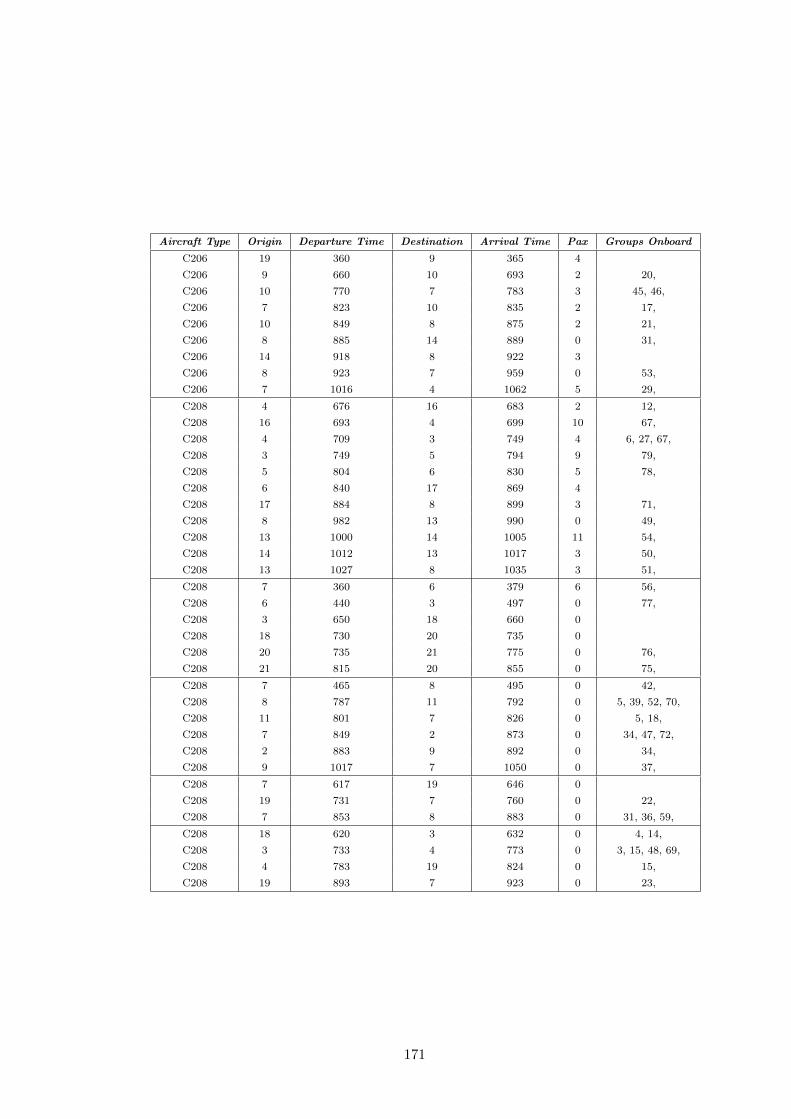
Aircraft Type Origin Departure Time Destination Arrival Time Pax Groups Onboard
C206 19 360 9 365 4
C206 9 660 10 693 2 20,
C206 10 770 7 783 3 45, 46,
C206 7 823 10 835 2 17,
C206 10 849 8 875 2 21,
C206 8 885 14 889 0 31,
C206 14 918 8 922 3
C206 8 923 7 959 0 53,
C206 7 1016 4 1062 5 29,
C208 4 676 16 683 2 12,
C208 16 693 4 699 10 67,
C208 4 709 3 749 4 6, 27, 67,
C208 3 749 5 794 9 79,
C208 5 804 6 830 5 78,
C208 6 840 17 869 4
C208 17 884 8 899 3 71,
C208 8 982 13 990 0 49,
C208 13 1000 14 1005 11 54,
C208 14 1012 13 1017 3 50,
C208 13 1027 8 1035 3 51,
C208 7 360 6 379 6 56,
C208 6 440 3 497 0 77,
C208 3 650 18 660 0
C208 18 730 20 735 0
C208 20 735 21 775 0 76,
C208 21 815 20 855 0 75,
C208 7 465 8 495 0 42,
C208 8 787 11 792 0 5, 39, 52, 70,
C208 11 801 7 826 0 5, 18,
C208 7 849 2 873 0 34, 47, 72,
C208 2 883 9 892 0 34,
C208 9 1017 7 1050 0 37,
C208 7 617 19 646 0
C208 19 731 7 760 0 22,
C208 7 853 8 883 0 31, 36, 59,
C208 18 620 3 632 0 4, 14,
C208 3 733 4 773 0 3, 15, 48, 69,
C208 4 783 19 824 0 15,
C208 19 893 7 923 0 23,
171
APPENDIX F Automated Composite
Schedule
172

Table F.1: Composite Variable Method Automated Full ScheduleAircraft Type Origin Departure Time Destination Arrival Time Pax Groups Onboard
C208 7 370 8 400 11 42,
C208 8 400 13 410 10 49,
C208 13 410 14 420 2 55,
C208 14 450 13 460 6 50,
C208 13 530 8 540 11 51,
C208 8 670 17 690 11
C208 17 690 8 710 8 71,
C208 8 770 11 790 7 52, 18,
C208 11 790 7 820 7
C208 7 860 2 890 4 72,
C208 2 900 19 910 4
C208 19 910 7 940 6 22,
C206 7 380 6 410 3 56,
C206 6 450 3 530 5 9,
C206 3 610 5 670 2 11,
C206 5 670 6 710 5 10,
C206 6 710 16 740 5
C206 16 740 3 800 4 67,
C206 3 860 4 920 5 74, 12,
C206 4 920 16 930 5
C206 7 380 11 420 4 58,
C206 11 490 2 500 4
C206 2 500 7 540 2 32,
C206 7 560 1 680 2
C206 1 690 2 820 3 73,
C206 2 860 9 880 3
C206 9 900 10 940 4 20,
C206 10 1060 7 1080 2 46,
C206 7 390 4 440 1 62,
C206 4 440 7 490 4 8,
C206 7 500 3 640 4 47, 19,
C206 3 670 19 770 2 15,
C206 19 770 9 780 2
C206 9 780 4 840 2 41,
C206 4 840 14 940 4 25, 31,
C206 14 950 13 960 4
C206 13 970 14 980 4 54,
C206 14 980 17 1000 4
C208 7 420 6 440 4
C208 6 480 3 540 11 77,
C208 3 760 18 780 2 7,
C208 18 780 3 800 6 4,
C208 3 800 5 850 11 79,
C208 5 850 6 880 11 78,
C208 6 900 15 910 11
C208 15 910 11 930 2 35,
C208 11 930 9 950 1 60,
C208 9 970 7 1010 11 37,
C206 8 490 7 530 3 33,
C206 7 590 8 630 5 59,
C206 8 670 12 800 4 68, 30,
C206 12 800 3 890 4
C206 3 890 18 910 2 26,
C206 18 910 3 930 2 14,
173
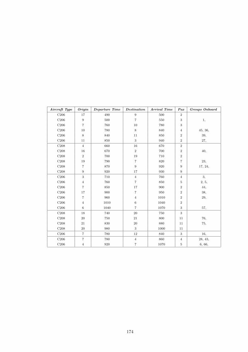
Aircraft Type Origin Departure Time Destination Arrival Time Pax Groups Onboard
C206 17 490 9 500 2
C206 9 500 7 550 3 1,
C206 7 760 10 780 3
C206 10 780 8 840 4 45, 36,
C206 8 840 11 850 2 39,
C206 11 850 3 940 2 27,
C208 4 660 16 670 2
C208 16 670 2 700 2 40,
C208 2 700 19 710 2
C208 19 790 7 820 7 23,
C208 7 870 9 920 9 17, 24,
C208 9 920 17 930 9
C206 3 710 4 760 4 3,
C206 4 760 7 850 5 2, 5,
C206 7 850 17 900 2 44,
C206 17 900 7 950 2 38,
C206 7 960 4 1010 2 29,
C206 4 1010 6 1040 2
C206 6 1040 7 1070 3 57,
C208 18 740 20 750 3
C208 20 750 21 800 11 76,
C208 21 830 20 880 11 75,
C208 20 980 3 1000 11
C206 7 780 12 840 3 16,
C206 7 780 4 860 4 28, 43,
C206 4 920 7 1070 5 6, 66,
174
APPENDIX G MVCVRP Data
G.1 Problem Data
175
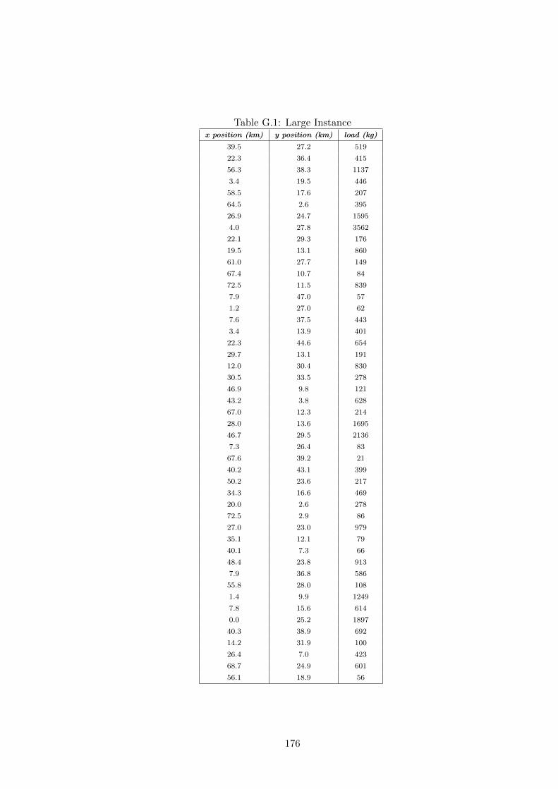
Table G.1: Large Instancex position (km) y position (km) load (kg)
39.5 27.2 519
22.3 36.4 415
56.3 38.3 1137
3.4 19.5 446
58.5 17.6 207
64.5 2.6 395
26.9 24.7 1595
4.0 27.8 3562
22.1 29.3 176
19.5 13.1 860
61.0 27.7 149
67.4 10.7 84
72.5 11.5 839
7.9 47.0 57
1.2 27.0 62
7.6 37.5 443
3.4 13.9 401
22.3 44.6 654
29.7 13.1 191
12.0 30.4 830
30.5 33.5 278
46.9 9.8 121
43.2 3.8 628
67.0 12.3 214
28.0 13.6 1695
46.7 29.5 2136
7.3 26.4 83
67.6 39.2 21
40.2 43.1 399
50.2 23.6 217
34.3 16.6 469
20.0 2.6 278
72.5 2.9 86
27.0 23.0 979
35.1 12.1 79
40.1 7.3 66
48.4 23.8 913
7.9 36.8 586
55.8 28.0 108
1.4 9.9 1249
7.8 15.6 614
0.0 25.2 1897
40.3 38.9 692
14.2 31.9 100
26.4 7.0 423
68.7 24.9 601
56.1 18.9 56
176

x position (km) y position (km) load (kg)
36.4 9.8 1051
7.1 27.7 588
68.6 4.6 987
20.2 41.0 100
20.2 31.7 217
6.7 1.5 1
58.5 14.0 202
35.6 12.0 1
3.3 22.7 1801
64.0 27.7 790
68.7 15.6 1136
6.0 29.8 514
71.1 5.4 105
45.9 16.3 134
35.5 10.3 425
9.7 1.4 1087
40.5 43.4 85
30.1 39.8 1036
49.8 33.9 716
25.1 23.3 358
51.5 8.4 69
40.2 38.3 375
31.6 23.9 99
45.8 23.0 478
65.6 17.4 834
21.7 7.1 162
16.5 27.5 473
64.8 22.5 43
50.6 35.1 826
57.9 7.6 471
15.0 45.0 2370
4.6 37.3 123
34.3 5.6 1037
12.9 2.3 140
39.4 26.4 520
34.6 35.1 82
29.5 42.4 507
6.6 29.8 1031
1.2 20.3 89
20.4 46.3 171
51.5 19.6 98
20.5 16.8 44
69.9 5.7 797
25.7 4.9 180
5.7 20.3 77
177
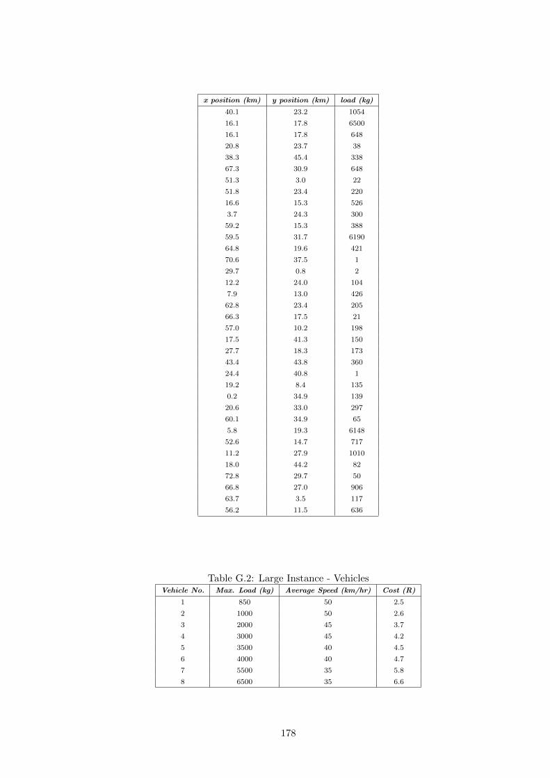
x position (km) y position (km) load (kg)
40.1 23.2 1054
16.1 17.8 6500
16.1 17.8 648
20.8 23.7 38
38.3 45.4 338
67.3 30.9 648
51.3 3.0 22
51.8 23.4 220
16.6 15.3 526
3.7 24.3 300
59.2 15.3 388
59.5 31.7 6190
64.8 19.6 421
70.6 37.5 1
29.7 0.8 2
12.2 24.0 104
7.9 13.0 426
62.8 23.4 205
66.3 17.5 21
57.0 10.2 198
17.5 41.3 150
27.7 18.3 173
43.4 43.8 360
24.4 40.8 1
19.2 8.4 135
0.2 34.9 139
20.6 33.0 297
60.1 34.9 65
5.8 19.3 6148
52.6 14.7 717
11.2 27.9 1010
18.0 44.2 82
72.8 29.7 50
66.8 27.0 906
63.7 3.5 117
56.2 11.5 636
Table G.2: Large Instance - VehiclesVehicle No. Max. Load (kg) Average Speed (km/hr) Cost (R)
1 850 50 2.5
2 1000 50 2.6
3 2000 45 3.7
4 3000 45 4.2
5 3500 40 4.5
6 4000 40 4.7
7 5500 35 5.8
8 6500 35 6.6
178

Table G.3: Medium Instance - Customersx position (km) y position (km) load (kg)
22.0 28.5 527
23.2 4.4 686
70.8 34.5 56
34.0 21.6 1401
30.4 33.2 6500
28.6 11.1 1037
5.2 37.1 637
24.6 19.7 6421
51.7 23.1 6500
25.2 7.2 6421
37.8 37.1 6500
25.6 45.2 2617
22.5 10.3 1036
66.1 5.3 6148
46.0 41.8 6500
24.3 25.3 5120
11.3 37.3 6421
40.2 3.4 1401
61.8 46.3 222
48.6 44.8 123
Table G.4: Medium Instance - VehiclesVehicle No. Max. Load (kg) Average Speed (km/hr) Cost (R)
1 850 50 2.5
2 2000 45 3.7
3 4000 40 4.7
4 6500 35 6.6
179

G.2 Supplied Delivery Lists
G.2.1 List for Day 1
nazareth house 207
garden village 311
meat good cash & carry 975
tacoma spur 173
warmbad rusoord maatskappy inc 459
supreme chicken centre 2737
bronco spar 278
stone craddle rietvlei 597
silverton sandwich bar 10
les marais spar 195
emperor’s palace 523
ciao baby cucina 47
cullinan sorg- en 1659
willow haven 250
tembisa hospital 1253
gerotek test facilities a 324
makhado correctional service 3943
fruit stop silverton 1080
multi meat & chicken wholesale 806
oasis lodge cc 693
rtt 462
dpt of correctional middelburg 1427
fringes 244
pax convenience stores 975
waterberg ouetehuis 349
medina meats 41
netcare optiklin hospital 154
fish 563
summit on site cc 444
f.h odendaal hospital 876
bergies take aways 87
mark slaghuis 161
goldreef city casino 392
arwyp medical centre 1611
180
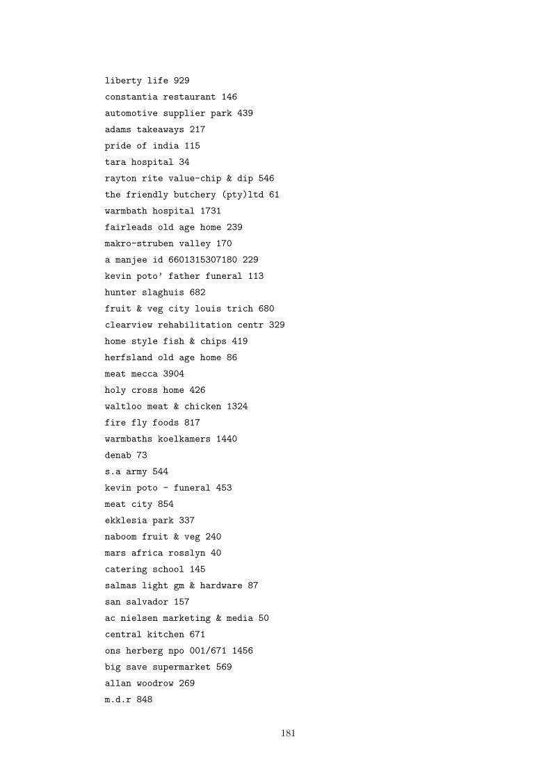
liberty life 929
constantia restaurant 146
automotive supplier park 439
adams takeaways 217
pride of india 115
tara hospital 34
rayton rite value-chip & dip 546
the friendly butchery (pty)ltd 61
warmbath hospital 1731
fairleads old age home 239
makro-struben valley 170
a manjee id 6601315307180 229
kevin poto’ father funeral 113
hunter slaghuis 682
fruit & veg city louis trich 680
clearview rehabilitation centr 329
home style fish & chips 419
herfsland old age home 86
meat mecca 3904
holy cross home 426
waltloo meat & chicken 1324
fire fly foods 817
warmbaths koelkamers 1440
denab 73
s.a army 544
kevin poto - funeral 453
meat city 854
ekklesia park 337
naboom fruit & veg 240
mars africa rosslyn 40
catering school 145
salmas light gm & hardware 87
san salvador 157
ac nielsen marketing & media 50
central kitchen 671
ons herberg npo 001/671 1456
big save supermarket 569
allan woodrow 269
m.d.r 848
181

putco mamelodi sbu 30
j.r. de abrco t/a blou bull 773
wimpy hatfield 53
tambo memorial hospital 3483
boston deli hazelwood 164
gerbera mess 339
main kitchen 982
mr munchies 776
a mess 5120
polokwane correctional service 7651
africafe 22
180 degrees done to perfection 572
national ceremonial gaurd 206
putco roseville 175
o’hagans 547
mario’s cash & carry 6529
crossroads recovery centre 96
sportlight gourmet foods 313
abedare cable edenvale 216
plot 32 173
4 sai 1362
bolivai lodge 686
engeneering formation 218
queens haven 237
ingwe single quarters 222
meat & veg chicken 283
peters supermarket foodzone 1447
sandfi aventis 478
roodepoort chicken wholesalers 762
kokanje aftree oord 1532
summit college 121
seafood delight 129
G.2.2 List for Day 2
forest farm 285
182
chatter box coffee cafe 173
magalies park 141
siemens wadeville 161
crawdaddys 96
centurion sub acute 44
s.a.bank note co. (pty)ltd 2021
samro 311
pineslopes spar 274
stone craddle rietvlei 1832
brpm hostel raasimone 29
tiberius fish shop 268
vibe catering 705
randjes park spar 234
promise grill restaurant 478
gallagher gourmet & catering c 1031
panarottis menlyn 141
prime co meat 2376
chamara trading cc (bosman) 2789
les marais spar 236
lafarge 157
la scala 692
big daddys 147
bondi distributors cc 2506
ann harding 125
bj’s the bridge 535
azinaz trading cc 9726
clicks distribution centre 102
millenium 189
clover sa 301
s.a.reserve bank 912
meat empire cc ck96/15394/23 265
gerotek test facilities 306
sizwe tropical disease hosp. 1104
banjaara 448
masakhane cookfreeze 9020
weskoppies hospital main kitch 3870
tumela hostel 3389
sandton foods 466
snoopy snacks 147
183
goldreef city casino 2352
arwyp medical centre 308
osalito centurion 65
npc staff restaurant 506
the raj indian restaurant 2617
mr salad 118
makro woodmead 224
p v b brits 836
tara hospital 186
dishaba hostel 1462
m s fernandes t/a target foods 1899
tip top meat products 1500
hernic ferrochrome mine 1690
platter xpress cc 222
quality meal services 276
emily hobhousetehuis 458
the friendly butchery (pty)ltd 101
health emporium & produce 1401
j.r. de abrco t/a blou bull 668
pretoria academic hospital 103
the sheiks palace 160
coco bonco 80
scrooge diner 410
baglios cc 506
sahil curry den 483
emperor foods 32
amandelbult hospital 75
papachinos clearwater 149
mars africa rosslyn 594
harry’s fast food centre cc 99
st martins school 305
frontline cash & carry 1557
mlanje hostel 1825
laudium meat supply 1000
bonnies fast foods 58
masonic haven 250
tuscan bbq groenkloof 1094
ons huis 103
lathyser fish and chips 418
184
central kitchen 216
tshwane university of technolo 278
matador w/salers 3211
clicks upd (roodeplaat) 385
ok value 6421
cosmic gold trd 368 579
pick n pay 422
boston deli hazelwood 637
ciao baby cucina 139
clayton house 121
africafe 579
serene park retirement village 510
kashif’s fusion food restaurant 88
ghazal bryanston 262
nathis catering 297
p.p.m training centre 195
nedbank selby ext 233
s.a.p college winkel 2163
nestle s.a 503
wolhuterskop trading 61
wimpy 1 4538
eugene marais creche 247
unisa florida campus 270
citadela 231
caternet pty ltd 7302
queens haven 289
barneys den supermarket 294
akeso parktown 310
ghazal north indain rest cc 49
king pie 852
casa bella guest 5
montina investment 728
meat net cc 285
parrots kolonade 229
germiston hospital 527
r p m rustenburg 176
desmondi campus catering 156
nampak rosslyn 285
bread basket franchise 135
185

jafta el kero old age 362
sanca horizon clinic 240
G.2.3 List for Day 3
nazareth house 519
huis vergendeg 415
ons tuis riveria 1137
fego student centre (main camp 446
north indian tansoor rest 207
setaria spar 395
the classic india restaurant 1595
s.a.p. hondeskool menasie 3562
gallegher gourmet catering 176
pretoria west hospital 860
ct fish market silverlakes 149
putco selby 84
vibe catering 839
the bread basket eastgate 57
panarottis menlyn 62
wang thai - sandton 443
masonic haven 401
chamara trading cc (bosman) 654
serenity aged home 191
les marais spar 830
clicks upd (roodeplaat) 278
deliver to ezulwini 121
detective academy 628
jaffa 214
azani caterers ck995487523 1695
tembisa hospital 2136
avalon 83
thava restaurant 21
gerotek test facilities a 399
oyo-restaurant 217
varsity bakery 469
bj’s the bridge 278
welkom mutchery 86
186
ghazal sunninghill 979
clicks distribution centre 79
mugg & bean 66
neptunes fishmonger 913
orient restaurant 586
librety life 108
gallagher gourmet & catering 1249
fish 614
igbal meat and deli 1897
a taste of punjab 692
nedbank 100 main 324
dawn 423
amor spyseniers 601
heidelburg graphics 56
goldreef city casino 1051
arwyp medical centre 588
retire@ midstream 987
crescent clinic 100
ebg sherwood trust (pty) ltd 217
wimpy no 1 548
liberty life 202
boom street no 1 1360
the raj indian restaurant 1801
mamelodi hospital 790
m s fernandes t/a target foods 1136
cape town fish market s/down 514
nedbank 105 west 263
excellent meat &chicken 134
platter xpress cc 425
ad-eed super market 1087
lorraine rautenback 85
engeneering formation 1036
staff hostel 716
east lynne spar 358
makro-struben valley 69
chazal bryanston 375
vetkoekden 99
norma & vilma caterers 478
emperor foods 834
187
rens butchery 162
so yum restaurant 473
papachinos clearwater 43
emperor’s palace 826
alberton meat market 471
bulk pack butchery 2370
a.g gooliman sons 123
fordsburg meat & supermarket c 1037
ekklesia park 140
klerksdorp tehuis vir bejaarde 520
d.c.l foods (pty) ltd 82
stabilis treatment centre 507
vista medi clinic 1031
del to ezulwini 89
van rensburg old age home 171
gafa huis protea home 98
fego lynwood 44
mf seafood distributors 797
js tikka & kebab 180
golden valley chineese rest 77
tambo memorial hospital 1054
a mess 7148
clayton house 38
five star caterers 338
africafe 648
sita 22
serene park retirement village 220
the sheiks palace 526
nathis catering 300
circle catering and 388
anglo platinum amandelbuilt 6190
akeso alberton 421
keg no 1 113
keg no 2 89
chazal north indain rest cc 104
desmondi campus catering 426
john dory’s fish & grill 205
21 signal mess 3952
skill moters 198
188

meat & veg chicken 150
akeso parktown 173
sandfi aventis 360
mc synty’s no 1 202
charles tiganis food enterpris 135
jubilee wits 139
ogalito centurion 297
armadillo’s coffee shop 65
swartklip mine 6148
the food factor 717
summit college 1010
bpr management services cc 82
ann harding 50
officer commanding 906
bread basket franchise 117
site park build (cafeteria) 636
189
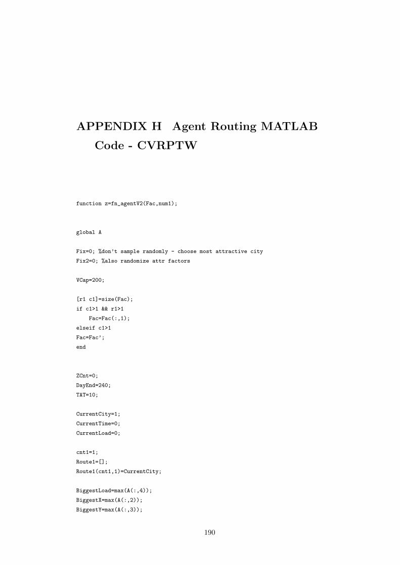
APPENDIX H Agent Routing MATLAB
Code - CVRPTW
function z=fn_agentV2(Fac,num1);
global A
Fix=0; %don’t sample randomly - choose most attractive city
Fix2=0; %also randomize attr factors
VCap=200;
[r1 c1]=size(Fac);
if c1>1 && r1>1
Fac=Fac(:,1);
elseif c1>1
Fac=Fac’;
end
ZCnt=0;
DayEnd=240;
TAT=10;
CurrentCity=1;
CurrentTime=0;
CurrentLoad=0;
cnt1=1;
Route1=[];
Route1(cnt1,1)=CurrentCity;
BiggestLoad=max(A(:,4));
BiggestX=max(A(:,2));
BiggestY=max(A(:,3));
190
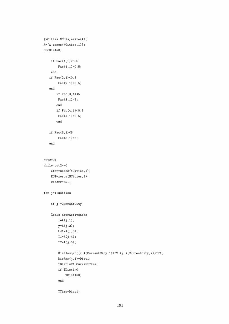
[NCities NCols]=size(A);
A=[A zeros(NCities,1)];
SumDis1=0;
if Fac(1,1)<0.5
Fac(1,1)=0.5;
end
if Fac(2,1)<0.5
Fac(2,1)=0.5;
end
if Fac(3,1)<5
Fac(3,1)=5;
end
if Fac(4,1)<0.5
Fac(4,1)=0.5;
end
if Fac(5,1)<5
Fac(5,1)=5;
end
out2=0;
while out2==0
Attr=zeros(NCities,1);
EDT=zeros(NCities,1);
DisArr=EDT;
for j=1:NCities
if j~=CurrentCity
%calc attractiveness
x=A(j,1);
y=A(j,2);
Ld1=A(j,3);
T1=A(j,4);
T2=A(j,5);
Dist1=sqrt((x-A(CurrentCity,1))^2+(y-A(CurrentCity,2))^2);
DisArr(j,1)=Dist1;
TDist1=T1-CurrentTime;
if TDist1<0
TDist1=0;
end
TTime=Dist1;
191

DDist1=sqrt((x-A(1,1))^2+(y-A(1,2))^2);
DTime=DDist1;
%can we get there on time?
%is load OK?
%can we get back to depot on time?
ArrTime=CurrentTime+TTime;
if ArrTime<T1
ArrTime=T1;
end
EDT(j,1)=ArrTime+TAT;
RetTime=EDT(j,1)+DTime;
if EDT(j,1)<T2 && CurrentLoad+Ld1<=VCap && RetTime<=DayEnd && (A(j,7)==0 || j==1)
%Bigger loads - more attractive
Close1=Ld1/BiggestLoad*Fac(1,1); % Fac(1) 1
if Close1<0.000001
stop1=1;
end
%closer - more attractive
Close2=Fac(2,1)*exp(-DDist1/Fac(3,1)); %Fac(2)~1.5 Fac(3)~10
%closer in time - more attractive
TDiff=EDT(j,1)-CurrentTime;
Close3=Fac(4,1)*exp(-TDiff/Fac(5,1)); %Fac(4)~1.5 Fac(5)~10
Attr(j,1)=Close1+Close2+Close3;
if j==1
Attr(j,1)=0;
end
end
end
end
AllZero=1;
for j=1:NCities
if Attr(j,1)>0.00000001
AllZero=0;
end
end
if AllZero==1
ZCnt=ZCnt+1;
192
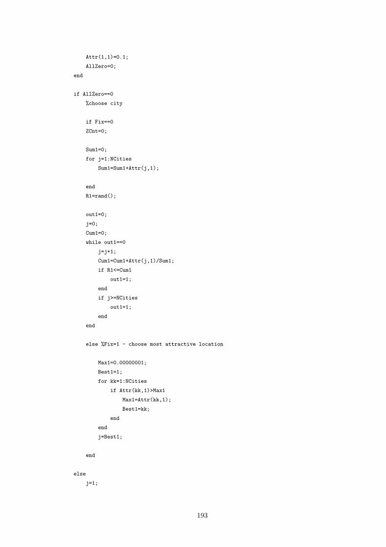
Attr(1,1)=0.1;
AllZero=0;
end
if AllZero==0
%choose city
if Fix==0
ZCnt=0;
Sum1=0;
for j=1:NCities
Sum1=Sum1+Attr(j,1);
end
R1=rand();
out1=0;
j=0;
Cum1=0;
while out1==0
j=j+1;
Cum1=Cum1+Attr(j,1)/Sum1;
if R1<=Cum1
out1=1;
end
if j>=NCities
out1=1;
end
end
else %Fix=1 - choose most attractive location
Max1=0.00000001;
Best1=1;
for kk=1:NCities
if Attr(kk,1)>Max1
Max1=Attr(kk,1);
Best1=kk;
end
end
j=Best1;
end
else
j=1;
193
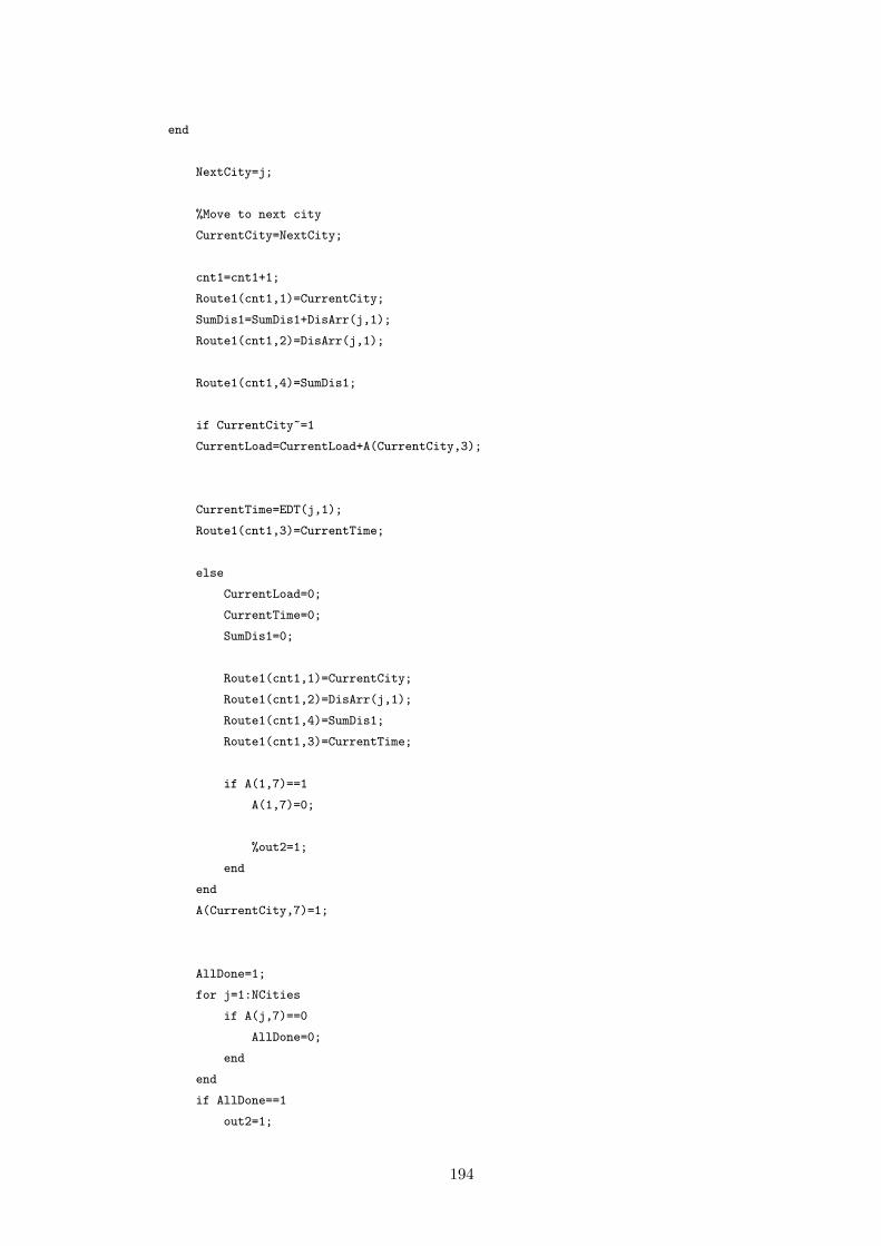
end
NextCity=j;
%Move to next city
CurrentCity=NextCity;
cnt1=cnt1+1;
Route1(cnt1,1)=CurrentCity;
SumDis1=SumDis1+DisArr(j,1);
Route1(cnt1,2)=DisArr(j,1);
Route1(cnt1,4)=SumDis1;
if CurrentCity~=1
CurrentLoad=CurrentLoad+A(CurrentCity,3);
CurrentTime=EDT(j,1);
Route1(cnt1,3)=CurrentTime;
else
CurrentLoad=0;
CurrentTime=0;
SumDis1=0;
Route1(cnt1,1)=CurrentCity;
Route1(cnt1,2)=DisArr(j,1);
Route1(cnt1,4)=SumDis1;
Route1(cnt1,3)=CurrentTime;
if A(1,7)==1
A(1,7)=0;
%out2=1;
end
end
A(CurrentCity,7)=1;
AllDone=1;
for j=1:NCities
if A(j,7)==0
AllDone=0;
end
end
if AllDone==1
out2=1;
194
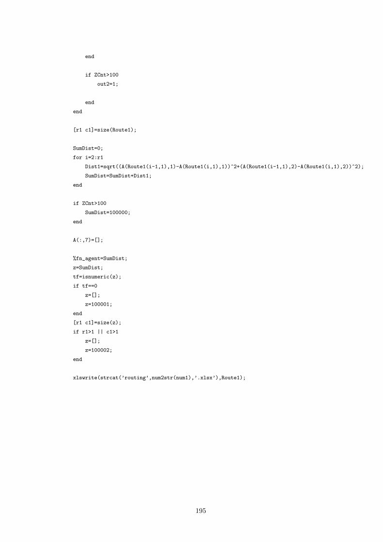
end
if ZCnt>100
out2=1;
end
end
[r1 c1]=size(Route1);
SumDist=0;
for i=2:r1
Dist1=sqrt((A(Route1(i-1,1),1)-A(Route1(i,1),1))^2+(A(Route1(i-1,1),2)-A(Route1(i,1),2))^2);
SumDist=SumDist+Dist1;
end
if ZCnt>100
SumDist=100000;
end
A(:,7)=[];
%fn_agent=SumDist;
z=SumDist;
tf=isnumeric(z);
if tf==0
z=[];
z=100001;
end
[r1 c1]=size(z);
if r1>1 || c1>1
z=[];
z=100002;
end
xlswrite(strcat(’routing’,num2str(num1),’.xlsx’),Route1);
195

APPENDIX I CVRPTW Data
196
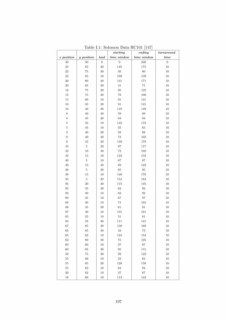
Table I.1: Solomon Data RC101 [147]starting ending turnaround
x position y position load time window time window time
40 50 0 0 240 0
25 85 20 145 175 10
22 75 30 50 80 10
22 85 10 109 139 10
20 80 40 141 171 10
20 85 20 41 71 10
18 75 20 95 125 10
15 75 20 79 109 10
15 80 10 91 121 10
10 35 20 91 121 10
10 40 30 119 149 10
8 40 40 59 89 10
8 45 20 64 94 10
5 35 10 142 172 10
5 45 10 35 65 10
2 40 20 58 88 10
0 40 20 72 102 10
0 45 20 149 179 10
44 5 20 87 117 10
42 10 40 72 102 10
42 15 10 122 152 10
40 5 10 67 97 10
40 15 40 92 122 10
38 5 30 65 95 10
38 15 10 148 178 10
35 5 20 154 184 10
95 30 30 115 145 10
95 35 20 62 92 10
92 30 10 62 92 10
90 35 10 67 97 10
88 30 10 74 104 10
88 35 20 61 91 10
87 30 10 131 161 10
85 25 10 51 81 10
85 35 30 111 141 10
67 85 20 139 169 10
65 85 40 43 73 10
65 82 10 124 154 10
62 80 30 75 105 10
60 80 10 37 67 10
60 85 30 85 115 10
58 75 20 92 122 10
55 80 10 33 63 10
55 85 20 128 158 10
55 82 10 64 94 10
20 82 10 37 67 10
18 80 10 113 143 10
197

starting ending turnaround
x position y position load time window time window time
2 45 10 45 75 10
42 5 10 151 181 10
42 12 10 104 134 10
72 35 30 116 146 10
55 20 19 83 113 10
25 30 3 52 82 10
20 50 5 91 121 10
55 60 16 139 169 10
30 60 16 140 170 10
50 35 19 130 160 10
30 25 23 96 126 10
15 10 20 152 182 10
10 20 19 42 72 10
15 60 17 155 185 10
45 65 9 66 96 10
65 35 3 52 82 10
65 20 6 39 69 10
45 30 17 53 83 10
35 40 16 11 41 10
41 37 16 133 163 10
64 42 9 70 100 10
40 60 21 144 174 10
31 52 27 41 71 10
35 69 23 180 210 10
65 55 14 65 95 10
63 65 8 30 60 10
2 60 5 77 107 10
20 20 8 141 171 10
5 5 16 74 104 10
60 12 31 75 105 10
23 3 7 150 180 10
8 56 27 90 120 10
6 68 30 89 119 10
47 47 13 192 222 10
49 58 10 86 116 10
27 43 9 42 72 10
37 31 14 35 65 10
57 29 18 96 126 10
63 23 2 87 117 10
21 24 28 87 117 10
12 24 13 90 120 10
24 58 19 67 97 10
67 5 25 144 174 10
37 47 6 86 116 10
49 42 13 167 197 10
53 43 14 14 44 10
61 52 3 178 208 10
198


![[adj.] crowded, modern, best, fast, most, close, British, quick [n.] journey, ferry, taxi, terminal, station, airline, distance, hour, way, fare [adv.]](https://static.fdocuments.net/doc/165x107/56649e155503460f94afff3f/adj-crowded-modern-best-fast-most-close-british-quick-n-journey.jpg)