arX

iv:h

ep-p

h/99

1043

5v3

10

Dec

199

9

VPI–IPPAP–99–09

Constraints on R–parity violating couplings from lepton

universality

Oleg Lebedev∗, Will Loinaz†, and Tatsu Takeuchi‡

Institute for Particle Physics and Astrophysics, Physics Department, Virginia Tech, Blacksburg,

VA 24061

(Revised : December 7, 1999)

Abstract

We analyze the one loop corrections to leptonic W and Z decays in an R–

parity violating extension to the Minimal Supersymmetric Standard Model

(MSSM). We find that lepton universality violation in the Z line–shape vari-

ables alone would strengthen the bounds on the magnitudes of the λ′ cou-

plings, but a global fit on all data leaves the bounds virtually unchanged at

|λ′33k| ≤ 0.42 and |λ′

23k| ≤ 0.50 at the 2σ level. Bounds from W decays are

less stringent: |λ′33k| ≤ 2.4 at 2σ, as a consequence of the weaker Fermilab

experimental bounds on lepton universality violation in W decays. We also

point out the potential of constraining R–parity violating couplings from the

measurement of the Υ invisible width.

12.60.Jv, 12.15.Lk, 13.38.Dg, 13.38.Be

Typeset using REVTEX

∗electronic address: lebedev@quasar.phys.vt.edu

†electronic address: loinaz@alumni.princeton.edu

‡electronic address: takeuchi@vt.edu

1

I. INTRODUCTION

The assumption of R–parity conservation in supersymmetric model-building has longbeen an economical means of (1) avoiding certain phenomenological problems in SUSYmodels (e.g. proton decay), (2) ensuring that the lightest supersymmetric particle is avail-able as a cure for the dark matter problem, and (3) reducing the SUSY model parameterspace. (For recent reviews, see Ref. [1].) However, the recent discovery of neutrino massat Super–Kamiokande [2] provides improved motivation for R–parity violating extensionsto the Minimal Supersymmetric Standard Model (MSSM). Detailed analyses of the phe-nomenological constraints on such models are thus warranted to quantify the amount ofR–parity violation permitted by current experimental data.

In this paper we consider the effects of R–parity violating extensions to the MSSM onlepton universality in W and Z decays. The R–conserving sector of the MSSM generateslepton universality violations proportional either to the lepton Yukawa couplings (due toHiggs interactions) or to the mass splittings of the sleptons (due to gauge interactions).Effects due to the Higgs sector will be considered in a future work [3] but will in general benegligible unless tanβ is quite large [4]. Effects due to gauge interactions are negligible if theslepton mass splittings are small. This is the case, for example, in supergravity (SUGRA)models with universal soft–breaking scalar masses at the SUGRA scale, in which the massdegeneracy is broken only by renormalization group running effects involving small Yukawacouplings. In R–parity violating models, however, R–parity violating interactions provideadditional sources of lepton universality violation which may be significantly larger thanthese smaller effects.

The R–parity violating superpotential has the following form:1

W6R =1

2λijkLiLjEk + λ′

ijkLiQjDk +1

2λ′′ijkUiDjDk , (1.1)

where Li, Ei, Qi, Ui, and Di are the MSSM superfields defined in the usual fashion [7], andthe subscript i = 1, 2, 3 is the generation index. Since a priori the interactions describedby this superpotential have an arbitrary flavor structure, we generically expect that in thecontext of W and Z decays these will give rise to lepton universality violations. In thispaper, we estimate the size of this violation and derive constraints on the R–parity violatingcouplings from LEP and Fermilab measurements of the leptonic observables in W and Zdecays.

It is clear that the purely baryonic operator UiDjDk is irrelevant to our discussion. Theother two operators may affect W and Z decays at one loop through vertex corrections to theWℓLν and ZℓLℓL vertices, with superparticles running in the loop. However, the couplingsλijk are already tightly constrained to be at most O(10−2), as the operator LiLjEk violateslepton universality in lepton decays at tree level [8]. The constraints on λ′

ijk are much lessstringent. Previous limits cite upper bounds on λ′

ijk as large as the gauge couplings (i.e.

1Because we are neglecting the soft breaking terms, we can rotate the bilinear terms away [5]. For

possible effects of the soft breaking terms on W and Z decays see Ref. [6].

2

as large as 0.5) with the SUSY scale at 100 GeV [1]. One may thus expect significantradiative corrections induced by these couplings. Henceforth we will focus on the effects ofthe operator LiQjDk only.

It is important to note that very strict constraints on the products of different R–violatingcouplings already exist from flavor-changing processes, e.g. µ → eγ constrains |λ′

1ijλ′2ij | <

4.6×10−4 [9]. However, these constraints can be easily satisfied by requiring only one of thesecouplings to be very small leaving the other coupling ill–constrained. The W and Z decayprocesses we consider here are flavor–conserving and involve the same R–violating couplingsquared. Thus we can constrain the individual couplings rather than their products.

We emphasize that, in the absence of a complete calculation in the full theory, focussingattention on the violation of lepton universality provides a clear advantage over studying theeffects of R–breaking couplings on the individual lepton–gauge boson couplings separately.This is because the R–conserving sector induces significant universal corrections to the leptoncouplings which depend strongly on the choice of SUSY parameters. These corrections (alongwith the corrections to the hadronic partial widths) cancel when considering violationsof lepton universality. Thus, the study of lepton universality violation lets us isolate theeffects of R–breaking interactions without ad hoc assumptions about corrections from theR–conserving sector.

In the following calculations we neglect left–right squark mixing. Left–right squarkmixing could be large only for the stop. However, since diagrams involving the stop containdown quarks with negligible mass, it will be seen that the contributions from these diagramsare numerically small (subleading in an expansion in m2

W or m2Z). Further, due to the chiral

structure of the R–breaking interactions, two left–right mass insertions would be requiredin the diagram. Thus, such contributions would be further suppressed as long as the mixingparameter is perturbatively small.

Radiative corrections to individual Z → ℓℓ partial widths due to R–breaking interactionshave previously been considered in Ref. [10] but lacked a consistent treatment of the R–conserving corrections. In this paper, we study the violation of lepton universality in Wand Z decay to isolate the effects of R–breaking couplings and constrain their sizes. Indetermining the limits on R–breaking from Z decay, we perform a global fit to all therelevant LEP and SLD observables in which the corrections from both R–breaking and R–conserving interactions are parametrized and fit to the data. This provides a consistentaccounting of R–conserving effects and allows us to improve the existing bounds on theR–breaking λ′ couplings. A companion study of constraints on λ′ and λ′′ couplings fromLEP/SLD hadronic observables has been performed in Ref. [11].

II. LEPTONIC W DECAYS

The relevant R–parity violating interactions expressed in terms of the component fieldstake the form

∆L 6R = λ′ijk

[

νiLdkRdjL + djLdkRνiL + d∗kRνciLdjL

−(eiLdkRujL + ujLdkReiL + d∗kReciLujL)

]

+ h.c. (2.1)

3

The one loop diagrams contributing to the decay W → eiLνi′L are shown in Figs. A 2 andA2. At one loop, the neutrino flavor may differ from that of the tree level vertex (i 6= i′)as a result of the R–parity violating interactions. Since neutrino flavor is indistinguishablein the detector, we should in principle sum over all three generations of antineutrino in thefinal state. However, since this is a one loop effect which does not interfere with the treelevel flavor conserving decay, we will neglect it in our analysis and set i = i′.

The amplitude of each diagram in Figs. A 2 and A2 are:

−NC |λ′ijk|2

[

−ig√2W µ(p+ q) eiL(p)γµνiL(q)

]

×

(1a) : 2 C24

(

0, 0, m2W ; 0, mujL

, mdjL

)

(1b) : (d− 2) C24

(

0, 0, m2W ;mdkR

, muj, 0)

−m2W C23

(

0, 0, m2W ;mdkR

, muj, 0)

(2a) : B1

(

0; 0, mujL

)

(2b) : B1

(

0; 0, mdjL

)

(2c) : B1

(

0;muj, mdkR

)

(2d) : B1

(

0; 0, mdkR

)

(2.2)

The expression in the square brackets is the tree level amplitude. The definitions of theintegrals B1, C23, and C24 are presented in the Appendix. In the above expressions NC = 3is the number of colors, and i, j, k are family indices; the final result must be summed overj and k to obtain the full correction for final state flavor i. We have set all the down typequark masses to zero. The up type quark masses muj

will also be set to zero except for thetop quark (j = 3, mu3

= mt).Combining the expressions in Eq. (2.2), with appropriate factors of 1

2for the wavefunction

renormalizations, we obtain the one–loop shift of the WeiLνiL coupling due to the λ′ijk

interaction:

δgijk = δg(u)ijk + δg

(d)ijk,

δg(d)ijk

g≡ −NC |λ′

ijk|2[

2 C24

(

0, mujL, mdjL

)

+1

2B1

(

0, mujL

)

+1

2B1

(

0, mdjL

)

]

,

δg(u)ijk

g≡ −NC |λ′

ijk|2[

(d− 2)C24

(

mdkR, muj

, 0)

−m2W C23

(

mdkR, muj

, 0)

+1

2B1

(

0, mdkR

)

+1

2B1

(

muj, mdkR

)

]

. (2.3)

We have suppressed the external momentum dependence of the B and C functions to sim-plify our expressions. The contributions of diagrams involving the down–type quark havebeen combined in δg

(d)ijk and those involving the up–type quark in δg

(u)ijk . The 1/ǫ poles of

dimensional regularization cancel separately in each of these combinations so they are finite.In the following, we evaluate the size of these shifts for a common squark mass of mq =

100 GeV. To facilitate estimations for different squark masses, we provide approximateformulae.

4

• First, we evaluate δg(u)i3k, the contribution from diagrams involving the top quark u3.

For mu3= mt = 175 GeV, mW = 81 GeV, and mq = 100 GeV, we find:

δg(u)i3k

g= −1.02% |λ′

i3k|2 (2.4)

An approximate expression can be obtained by expanding the full expression of δg(u)i3k

in powers of m2W :

δg(u)i3k

g≈ − NC

(4π)2|λ′

i3k|2

×[

x

4(1− x)2

{

x− 1− (2− x) ln x}

+m2

W

m2t

x

3(1− x)2

{

1− x+ ln x}

]

(2.5)

where x = m2t/m

2q . For mq = 100 GeV, this expression is equal to (−1.11 +

0.09)% |λ′i3k|2. Compared to the exact result above, we see that the leading order

approximation is already fairly accurate.

• The contributions of the diagrams with massless quarks are numerically smaller andvanish as mW → 0. The correction with massless up-type quarks (j = 1, 2) is:

δg(u)ijk

g= 0.22% |λ′

ijk|2 (j = 1, 2) (2.6)

The approximate form to leading order in m2W/m2

q is

δg(u)ijk

g≈ NC

(4π)2|λ′

ijk|2m2

W

9m2q

(

1− 3 lnm2

W

m2q

)

. (2.7)

For mq = 100 GeV, this gives 0.31% |λ′ijk|2 which suffices for our purpose.

• The diagrams with down–type quarks contribute:

δg(d)ijk

g= 0.07% |λ′

ijk|2 (2.8)

the approximate expression being

δg(d)ijk

g≈ NC

(4π)2|λ′

ijk|2(

m2W

18m2q

)

. (2.9)

For mq = 100 GeV, this gives 0.07% |λ′ijk|2 to the accuracy shown.

5

Note that each contribution, Eqns. (2.5), (2.7), and (2.9) separately decouples in the limitm2

q → ∞ as they should. Collecting everything together, the shift in the coupling of thei–th generation lepton to the W is given by:

δgig

=∑

j,k

δg(u)ijk

g+

δg(d)ijk

g

= −0.95%∑

k

|λ′i3k|2 + 0.29%

∑

k

|λ′i2k|2 + 0.29%

∑

k

|λ′i1k|2 (2.10)

where we have summed over all possible generation indices j and k.The current bound on lepton universality violation in leptonic W decays from D0/ is [13]

gτge

= 1.004± 0.019(stat.)± 0.026(syst.).

This places a constraint on

δ

(

gτge

)

=δg3g

− δg1g

. (2.11)

Note that R–conserving corrections do not contribute since they cancel in the ratio gτ/ge.The constraint on the R–breaking couplings is thus

−0.4± 1.9(stat.)± 2.6(syst.)

={

∑

k

|λ′33k|2 − 0.3

∑

k

|λ′32k|2 − 0.3

∑

k

|λ′31k|2

}

−{

∑

k

|λ′13k|2 − 0.3

∑

k

|λ′12k|2 − 0.3

∑

k

|λ′11k|2

}

. (2.12)

Of the couplings λ′ijk appearing in this expression, the i = 1 couplings are already well

constrained from neutrino–less double beta decay, neutrino masses, atomic parity violation,and low energy charged current universality. Using the 2σ limits for the individual couplingscharted in Ref. [14], we find for mq = 100 GeV:

∑

k

|λ′11k|2 ≤ 0.00088,

∑

k

|λ′12k|2 ≤ 0.0055,

∑

k

|λ′13k|2 ≤ 0.079. (2.13)

The i = 3, j = 1 couplings are also well constrained from Rτπ = Γ(τ → πντ )/Γ(π → µνµ).Again, using the 2σ limits cited in Ref. [14] we find

∑

k

|λ′31k|2 ≤ 0.036 (2.14)

Therefore, we can neglect the λ′1jk and λ′

31k terms in Eq. (2.12) and obtain

∑

k

|λ′33k|2 − 0.3

∑

k

|λ′32k|2 = −0.4± 3.2 (2.15)

6

where the systematic and statistical errors have been added in quadrature. If we neglect the32k term with a smaller numerical coefficient, this places a 1σ (2σ) upper bound on the 33kterm:

∑

k

|λ′33k|2 ≤ 2.8 (6.0), (2.16)

which in turn translates into the limit

|λ′33k| ≤ 1.7 (2.4). (2.17)

Non–zero values of λ′32k will weaken this bound.

As we will see later, Z decay data places a constraint on∑

k |λ′33k|2 at the ±0.1 level.

Therefore, for the W decay data to be competitive with the Z decay data, the error mustbe improved by more than an order of magnitude. While the Tevatron Run II may provideenough data to improve the statistical error considerably, improving the systematic errormay prove a challenge [15].

III. LEPTONIC Z DECAYS

We next consider the effect of R–parity violating interactions on flavor–conserving lep-tonic Z decays, Z → eiLeiL. Note that the λ′ interaction in Eq. (1.1) involves only theleft–handed lepton field. Therefore, at the one–loop level the right–handed coupling is un-affected. Neglecting all down–type quark masses, the amplitudes of the diagrams shown inFigs. A 2 and A2 are

−NC |λ′ijk|2

[

−ig

cos θWZµ(p+ q) eiL(p)γµeiL(q)

]

×

(3a) : −2huLC24

(

0, 0, m2Z ; 0, mujL

, mujL

)

(3b) : +2hdRC24

(

0, 0, m2Z ;muj

, mdkR, mdkR

)

(3c) : −huL

[

(d− 2)C24

(

0, 0, m2Z ;mdkR

, muj, muj

)

−m2ZC23

(

0, 0, m2Z ;mdkR

, muj, muj

)]

(3d) : +hdR

[

(d− 2)C24

(

0, 0, m2Z ;mujL

, 0, 0)

−m2ZC23

(

0, 0, m2Z ;mujL

, 0, 0)]

(3e) : huRm2

ujC0

(

0, 0, m2Z ;mdkL

, muj, muj

)

(4a) + (4b) : 2heLB1

(

0; 0, mujL

)

(4c) + (4d) : 2heLB1

(

0;muj, mdkR

)

(3.1)

where

hfL = I3 −Qf sin2 θW , hfR = −Qf sin

2 θW . (3.2)

The tree level amplitude is heL times the expression in the square brackets. These correctionscan be expressed as a shift in the coupling heL:

7

δhijk = δh(u)ijk + δh

(d)ijk

δh(d)ijk ≡ −NC |λ′

ijk|2[

− 2huLC24

(

0, mujL, mujL

)

+hdR

{

(d− 2)C24

(

mujL, 0, 0

)

−m2ZC23

(

mujL, 0, 0

)}

+heLB1

(

0, mujL

)

]

δh(u)ijk ≡ −NC |λ′

ijk|2[

2hdRC24

(

muj, mdkR

, mdkR

)

−huL

{

(d− 2)C24

(

mdkR, muj

, muj

)

−m2ZC23

(

mdkR, muj

, muj

)}

+huRm2

ujC0

(

mdkL, muj

, muj

)

+heLB1

(

muj, mdkR

)

]

(3.3)

Again, the dependence on the external momenta has been suppressed. The corrections whichdepend on the down–type quark have been grouped together in δh

(d)ijk and those that depend

on the up–type quark in δh(u)ijk. These combinations are separately finite. For simplicity, we

again evaluate these shifts for a common squark mass of mq = 100 GeV.

• We begin with the top quark dependent contribution. For mt = 175 GeV, mZ =92 GeV, and mq = 100 GeV, we find

δh(u)i3k = 0.63% |λ′

i3k|2. (3.4)

This is well approximated by the leading mZ = 0 piece of the expansion in the Z mass:

δh(u)ijk ≈ − NC

2(4π)2|λ′

i3k|2 F (x) (3.5)

where

F (x) =x

1− x

(

1 +1

1− xln x

)

(3.6)

and x = m2t/m

2q. For mq = 100 GeV, this gives 0.65% |λ′

i3k|2. The subleading terms

from the individual diagrams contributing to δh(u)i3k are:

(3b) : −NC hdR

(4π)2|λ′

i3k|2m2

Z

2m2q

f(

1

x

)

(3c) :NC huL

(4π)2|λ′

i3k|2m2

Z

m2t

f(x)

(3e) : −NC huR

(4π)2|λ′

i3k|2m2

Z

m2t

g(x) (3.7)

where

8

f(x) ≡ − 1

18

1

(1− x)4

[

2x4 − 9x3 + 18x2 − 11x− 6x ln x]

(3.8)

g(x) ≡ 1

12

1

(1− x)4

[

x4 − 6x3 + 3x2 + 2x+ 6x2 ln x]

(3.9)

The total subleading contribution for mq = 100 GeV is −0.03% |λ′ijk|2.

In Ref. [10], the leading and subleading contributions of diagrams (3b) and (3c) areshown2 but the subleading contribution of diagram (3e) appears to have been omitted.We also disagree with the expression for (3b) in Ref. [10] by a factor of 1

2. However,

the numerical impact is negligible.

• The corrections involving massless quark loops vanish in the limit mZ → 0 and givenumerically small contributions. For the massless up–type quarks (u1 = u and u2 = c)we find:

δh(u)ijk = −0.02% |λ′

ijk|2. (3.10)

The leading order term in m2Z/m

2q is

δh(u)ijk ≈ − NC

(4π)2|λ′

ijk|2[

huL

m2Z

9m2q

(

1− 3 lnm2

Z

m2q

)

− hdR

m2Z

18m2q

]

. (3.11)

For mq = 100 GeV, this gives −0.01% |λ′ijk|2.

• The massless down–type quark dependent correction is:

δh(d)ijk = −0.06% |λ′

ijk|2 (3.12)

The leading order term in m2Z/m

2q is

δh(d)ijk ≈ − NC

(4π)2|λ′

ijk|2[

huL

m2Z

18m2q

− hdR

m2Z

9m2q

(

1− 3 lnm2

Z

m2q

)]

(3.13)

For mq = 100 GeV, this gives −0.09% |λ′ijk|2.

Combining everything together, and summing over the generation indices j and k, theshift of the i–th generation lepton coupling to the Z due to R–violating interactions is:

δh6Ri =

∑

j,k

[

δh(u)ijk + δh

(d)ijk

]

= 0.61%∑

k

|λ′i3k|2 − 0.08%

∑

k

|λ′i2k|2 − 0.08%

∑

k

|λ′i1k|2

≈ 0.61%∑

k

|λ′i3k|2 (3.14)

where we drop the subleading terms. (This is equivalent to keeping only the diagramsinvolving the top and the stop.).

2cf Eq. 9 of Ref. [10].

9

IV. FITS AND NUMERICAL ANALYSES

In order to place limits on the λ′ijk couplings from Z decay, we need to know how the

observables at LEP and SLD will be affected by the shifts δh6Ri in the left–handed coupling

of ei to the Z, as well as by other R–conserving vertex and oblique corrections.The relevant observables are

Rℓ =Γ(Z → hadrons)

Γ(Z → ℓ+ℓ−)=

NC

∑

q=u,d,s,c,b(h2qL

+ h2qR)

(h2ℓL

+ h2ℓR)

(4.1)

and

Aℓ =h2ℓL

− h2ℓR

h2ℓL

+ h2ℓR

(4.2)

as well as

AFB(ℓ) =3

4AeAℓ (4.3)

where ℓ = e, µ, τ . The shift in Rℓ due to shifts in the coupling constants is

δRℓ

Rℓ

=δΓhad

Γhad− 2hℓLδhℓL + 2hℓRδhℓR

h2ℓL

+ h2ℓR

= ∆R − 2hℓL

h2ℓL

+ h2ℓR

δh6Rℓ

= ∆R + 4.3 δh6Rℓ (4.4)

where we have subsumed all the hadronic corrections and the lepton flavor independentoblique and vertex corrections into a single parameter ∆R, and the coefficient of δh6R

ℓ iscalculated for the value sin2 θW = 0.2315.

We note that the λ′ couplings we are trying to constrain also contribute to ∆R throughΓhad since they modify the Zqq vertices3 as well as the Zℓℓ vertices. However, since ∆R

also subsumes highly model dependent corrections from the R–conserving sector, it can beconsidered an independent parameter from δh6R

ℓ in our fit.Similarly, the shift in Aℓ is given by

δAℓ

Aℓ

=4hℓLh

2ℓRδhℓL − 4h2

ℓLhℓRδhℓR

h4ℓL

− h4ℓR

= ∆A +4hℓLh

2ℓR

h4ℓL

− h4ℓR

δh6Rℓ

= ∆A − 25 δh6Rℓ (4.5)

3The flavor dependence of R–violating corrections to the Zqq vertices can be used to constrain λ′

and λ′′ by looking at purely hadronic observables [11].

10

where we have subsumed all the lepton flavor independent oblique and vertex correctionsinto a single parameter ∆A, and the coefficient of δh6R

ℓ is again calculated for the valuesin2 θW = 0.2315. We do not need to introduce another flavor independent parameter forAFB(ℓ) since

δAFB(ℓ)

AFB(ℓ)=

δAe

Ae

+δAℓ

Aℓ

= 2∆A − 25 δh6Re − 25 δh6R

ℓ . (4.6)

Therefore, we can express all corrections from both R–breaking and R–conserving interac-tions in terms of just 5 parameters: ∆R, ∆A, and δh6R

ℓ , ℓ = e, µ, τ . A five parameter fitcannot be conducted, however, since a change in any one parameter can always be absorbedinto the other four. We therefore define

∆Re≡ ∆R + 4.3 δh6R

e ,∆Ae

≡ ∆A − 25 δh6Re ,

δµe ≡ δh6Rµ − δh6R

e ,

δτe ≡ δh6Rτ − δh6R

e . (4.7)

and perform a four parameter fit instead. Note that the parameters

δµe = 0.61%

{

∑

k

|λ′23k|2 −

∑

k

|λ′13k|2

}

δτe = 0.61%

{

∑

k

|λ′33k|2 −

∑

k

|λ′13k|2

}

(4.8)

are measures of lepton universality violation. The dependence of all the observables we usein our fit to the four fit parameters is:

δRe

Re

= ∆Re

δRµ

Rµ

= ∆Re+ 4.3 δµe

δRτ

Rτ

= ∆Re+ 4.3 δτe

δAe

Ae

= ∆Ae

δAµ

Aµ

= ∆Ae− 25 δµe

δAτ

Aτ

= ∆Ae− 25 δτe

δAFB(e)

AFB(e)= 2∆Ae

δAFB(µ)

AFB(µ)= 2∆Ae

− 25 δµe

δAFB(τ)

AFB(τ)= 2∆Ae

− 25 δτe (4.9)

11

In table I, we show the most recent data of these observables from Refs. [16], [17],and [18]. The Standard Model predictions were calculated by ZFITTER v6.21 [19] withstandard flag settings for the input values of mt = 174.3 GeV [20], mH = 300 GeV, andαs(mZ) = 0.120. The limits on lepton universality violation is insensitive to the choiceof the Higgs mass since Higgs couplings within the Standard Model do not violate leptonuniversality by any appreciable amount. The correlation matrix of the LEP Z lineshapedata is shown in table II.

The result of the four parameter fit to all the data in table I is

δµe = 0.00038± 0.00056δτe = −0.00013± 0.00061

∆Ae= 0.052 ± 0.012

∆Re= 0.0007± 0.0020 (4.10)

with the correlation matrix shown in table III. The quality of the fit was χ2 = 8.3/(12− 4).In figures 5 and 6 we show the 1σ constraints placed on δµe and δτe in the ∆Ae

= ∆Re= 0

plane by each observable. It is seen that the strongest constraints come from Rµ, Rτ , andAτ from the τ polarization measurement at LEP. In figure 7, we show the 68% and 90%confidence contours on the δµe–δτe plane.

The limits on δµe and δτe translate into limits on the R–breaking couplings:

∑

k

|λ′23k|2 −

∑

k

|λ′13k|2 = 0.062± 0.093

∑

k

|λ′33k|2 −

∑

k

|λ′13k|2 = −0.02 ± 0.10

∑

k

|λ′33k|2 −

∑

k

|λ′23k|2 = −0.083± 0.093 (4.11)

If we neglect the 13k terms since they are already constrained to be small (recall thatEq. (2.13) shows the 2σ upper bound), we obtain the following 1σ (2σ) upper bounds forthe 23k and 33k terms:

∑

k

|λ′23k|2 ≤ 0.16 (0.25)

∑

k

|λ′33k|2 ≤ 0.08 (0.18) (4.12)

or

|λ′23k| ≤ 0.40 (0.50)

|λ′33k| ≤ 0.28 (0.42) (4.13)

The limit on λ′23k should be interpreted as a limit on λ′

232 since λ′231 and λ′

233 are alreadyfairly well constrained by other experiments [14]. If any of the 13k–terms (in particular,λ′132 with a 2σ upper bound of 0.28 [14]) are non–zero, these limits will be weakened.It is interesting to note that since the measured value of Rτ is smaller than the measured

value of Re, this pair prefers a negative value of δτe (cf. Eq. 4.9). The same can be said ofthe pair AFB(e) and AFB(τ). On the other hand, the measured values of Ae (LEP and SLD)

12

and ALR are all larger than the measured values of Aτ (LEP and SLD) so these observablesprefer a positive value of δτe. (This is not apparent in figures 5 and 6 since they show theconstraints in the ∆Ae

= 0 plane.) Due to this conflict, the central value of δτe preferred bythe global fit is virtually zero which satisfies neither the R’s nor the A’s. In fact, Aτ fromLEP, with its smaller fractional error, actually accounts for 2.8 out of 6.8 of the χ2 of thefit.

If we perform our fit on the six Z line–shape parameters only, the result is

δµe = 0.00002± 0.00061δτe = −0.00082± 0.00070

∆Ae= 0.055 ± 0.033

∆Re= 0.0022± 0.0022 (4.14)

with χ2 = 1.9/(6− 4), and the correlation matrix is shown in table IV. The 90% confidencecontour in the δµe–δτe plane is shown in figures 7 and 8. This translates into

∑

k

|λ′23k|2 −

∑

k

|λ′13k|2 = 0.00± 0.10

∑

k

|λ′33k|2 −

∑

k

|λ′13k|2 = −0.13 ± 0.11

∑

k

|λ′33k|2 −

∑

k

|λ′23k|2 = −0.138± 0.097 (4.15)

Again, neglecting the 13k term, we obtain the following 1σ (2σ) limits:

∑

k

|λ′23k|2 ≤ 0.10 (0.20)

∑

k

|λ′33k|2 ≤ −0.02 (0.09) (4.16)

or

|λ′23k| ≤ 0.37 (0.49)

|λ′33k| ≤ (0.30) (4.17)

The negative central value for δτe leads to a reduced upper bound for |λ′33k|.

If we perform our fit on the two τ–polarization observables and the four SLD observablesonly, the result is:

δµe = 0.0040± 0.0046δτe = 0.0025± 0.0013

∆Ae= 0.062± 0.013 (4.18)

with χ2 = 0.84/(6−3), and the correlation matrix is shown in table V. The 90% confidencecontour in the δµe–δτe plane for this case is also shown in figures 7 and 8. This translatesinto

∑

k

|λ′23k|2 −

∑

k

|λ′13k|2 = 0.66± 0.75

13

∑

k

|λ′33k|2 −

∑

k

|λ′13k|2 = 0.41± 0.22

∑

k

|λ′33k|2 −

∑

k

|λ′23k|2 = −0.25± 0.77 (4.19)

Neglecting the 13k term, we obtain the following 1σ (2σ) limits:

∑

k

|λ′23k|2 ≤ 1.4 (2.2)

∑

k

|λ′33k|2 ≤ 0.62 (0.85) (4.20)

or

|λ′23k| ≤ 1.2 (1.5)

|λ′33k| ≤ 0.79 (0.92) (4.21)

This time, the upper bounds are considerably larger.This shows that had we used only the Z line–shape variables, which has been the case in

previous analyses by other authors [10,12], or only the leptonic asymmetries, we would havereached drastically different conclusions concerning the limits on the R–breaking parameters.Only through a global analysis were we able to constrain the parameters in a consistent way.

V. SUMMARY AND CONCLUSIONS

We find that flavor-conserving leptonic Z and W decays can be used to place significantconstraints on the size of R–parity violating λ′ couplings. Current bounds from leptonuniversality violation in leptonic Z decays from combined LEP/SLD data are

|λ′23k| ≤ 0.40 (0.50)

|λ′33k| ≤ 0.28 (0.42) (5.1)

at the 1σ (2σ) level, assuming a common squark mass of mq = 100 GeV and the sup-pression of λ′

13k couplings. For larger (common) squark masses the above bounds should

be interpreted as bounds on |λ′| ×√

F (x)/F (x0), where F (x) is defined in Eq. 3.6 and

x0 =m2

t

(100GeV)2.

Numerically, our numbers are not a significant improvement over those cited in Ref. [14].However, the methods used to derive previous limits [10,12] were intrinsically flawed in that(1) R–conserving effects were not properly taken into account and (2) R–breaking effectson only the leptonic widths of the Z were considered. Indeed, had we also considered onlythe leptonic widths, our limits would have been those of Eq. (4.17). The analysis of thispaper avoids these problems by focussing on lepton universality violation and performinga global fit on all LEP/SLD observables. The R–conserving effects are taken into accountby parametrizing and fitting them to the data also. (Similar methods have been used inRef. [21] to constrain flavor specific vertex corrections while taking into account the flavoruniversal oblique corrections.)

Current bounds on lepton universality in leptonic W decays provides the constraint

14

|λ′33k| ≤ 1.7 (2.4) (5.2)

at the 1σ (2σ) level. While not currently competitive with the Z decay bounds, the Fermilabresults are complementary independent measurements, and they can be expected to improvedramatically at Tevatron Run II.

If the error on the LEP/SLD observables continue to shrink with the current centralvalues, then eventually the region allowed by the line–shape variables and the asymmetrieswill fail to overlap in figure 8. In such a situation, not only the SM but the MSSM withR–parity violating couplings would be ruled out. In fact, no theory which introduces leptonuniversality violation in only the left–handed couplings would be viable.

Currently, the LEP and SLD observable provide the best limits on the λ′33k couplings.

However, one can potentially place a limit on the λ′ couplings by looking at invisible decaysof the Υ and J/Ψ resonances at the B and τ–charm factories [22]. The current bounds on λ′

i33

imply that the correction to the invisible width of the Υ resonance can be as large as 30%.A rough estimate shows that if the Υ invisible width is found to agree with the StandardModel prediction with 5% accuracy, the λ′ coupling would be constrained to be |λ′

i33| ≤ 0.16at the 2σ level. In addition, constraints on |λ′

333| will be available from forthcoming Tevatronstudies of the decay t → τb [23].

ACKNOWLEDGMENTS

We thank Morris Swartz and Robert Clare for providing us with the latest LEP-EWWG data including the correlation matrices. Helpful communications with GautamBhattacharyya, James E. Brau, Herbi Dreiner, Apostolos Pilaftsis, Franco Rimondi, andPeter Rowson are also gratefully acknowledged. We thank the hospitality of the FermilabParticle Theory Group, where part of this work was conducted under the auspices of theSummer Visitors’ Program. This work was supported in part (O.L. and W.L.) by the U. S.Department of Energy, grant DE-FG05-92-ER40709, Task A.

15

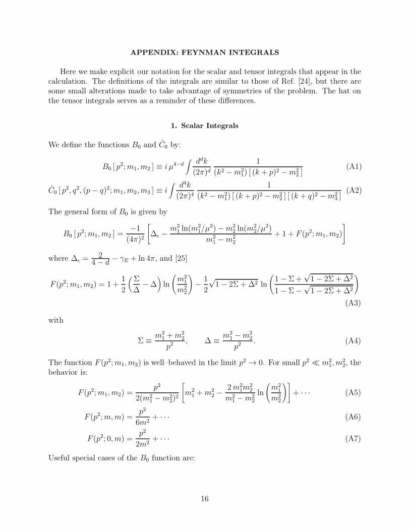
APPENDIX: FEYNMAN INTEGRALS

Here we make explicit our notation for the scalar and tensor integrals that appear in thecalculation. The definitions of the integrals are similar to those of Ref. [24], but there aresome small alterations made to take advantage of symmetries of the problem. The hat onthe tensor integrals serves as a reminder of these differences.

1. Scalar Integrals

We define the functions B0 and C0 by:

B0 [ p2;m1, m2 ] ≡ i µ4−d

∫

ddk

(2π)d1

(k2 −m21) [ (k + p)2 −m2

2 ](A1)

C0 [ p2, q2, (p− q)2;m1, m2, m3 ] ≡ i

∫

d4k

(2π)41

(k2 −m21) [ (k + p)2 −m2

2 ] [ (k + q)2 −m23 ]

(A2)

The general form of B0 is given by

B0 [ p2;m1, m2 ] =

−1

(4π)2

[

∆ǫ −m2

1 ln(m21/µ

2)−m22 ln(m

22/µ

2)

m21 −m2

2

+ 1 + F (p2;m1, m2)

]

where ∆ǫ =2

4− d − γE + ln 4π, and [25]

F (p2;m1, m2) = 1 +1

2

(

Σ

∆−∆

)

ln

(

m21

m22

)

− 1

2

√1− 2Σ +∆2 ln

(

1− Σ+√1− 2Σ +∆2

1− Σ−√1− 2Σ +∆2

)

(A3)

with

Σ ≡ m21 +m2

2

p2, ∆ ≡ m2

1 −m22

p2. (A4)

The function F (p2;m1, m2) is well–behaved in the limit p2 → 0. For small p2 ≪ m21, m

22, the

behavior is:

F (p2;m1, m2) =p2

2(m21 −m2

2)2

[

m21 +m2

2 −2m2

1m22

m21 −m2

2

ln

(

m21

m22

)]

+ · · · (A5)

F (p2;m,m) =p2

6m2+ · · · (A6)

F (p2; 0, m) =p2

2m2+ · · · (A7)

Useful special cases of the B0 function are:

16

B0 [ p2;m,m ] =

−1

(4π)2

∆ǫ − lnm2

µ2+ 2−

√

1− 4m2

p2ln

√

1− 4m2

p2+ 1

√

1− 4m2

p2− 1

(A8)

B0 [ p2; 0, m ] =

−1

(4π)2

[

∆ǫ − lnm2

µ2+ 2−

(

1− m2

p2

)

ln

(

1− p2

m2

)]

(A9)

The general form of the C0 function is fairly complex and we refer the reader to Ref. [24].It simplifies considerably for the following cases:

C0 [ 0, 0, p2;m, 0, 0 ] =

−1

(4π)21

p2

[

ln

(

p2

m2

)

ln

(

1 +p2

m2

)

+ Li2

(

− p2

m2

) ]

(A10)

C0 [ 0, 0, p2; 0, m1, m2 ] =

−1

(4π)21

4p2

[

ln2

(

1− Σ+√1− 2Σ +∆2

1− Σ−√1− 2Σ +∆2

)

− ln2

(

m21

m22

)]

(A11)

where Σ and ∆ are defined as in Eq. (A4).The following C0 could be expressed in terms a sum of dilogarithms, but for our pur-

poses it is simpler to reduce them to a Feynman parameter integral and either perform theintegration numerically or, if an expansion is needed, to expand the integrand directly andthen integrate.

C0 [ 0, 0, p2;m,M, 0 ] =

1

(4π)2

∫ 1

0dx

1

p2(1− x) +m2ln

[

(m2 −M2)x+M2

(1− x)(M2 − xp2)

]

(A12)

C0 [ 0, 0, p2;m,M,M ] =

1

(4π)2

∫ 1

0dx

1

p2(1− x) + (m2 −M2)ln

[

(m2 −M2)x+M2

−p2x(1− x) +M2

]

(A13)

2. Tensor Integrals

Definition and general form of B1:

Bµ [ p;m1, m2 ] = iµ4−d∫

ddk

(2π)dkµ

(k2 −m21) [(k + p)2 −m2

2]≡ pµB1 [ p

2;m1, m2 ] (A14)

B1 [ p2;m1, m2 ] = −1

2B0 [ p

2;m1, m2 ] +1

(4π)2

(

m21 −m2

2

2p2

)

F (p2;m1, m2) (A15)

¿From Eq. (A5), we find that in the limit p2 → 0:

B1 [ 0;m1, m2 ] = −1

2B0 [ 0;m1, m2 ] +

1

(4π)21

4(m21 −m2

2)

[

m21 +m2

2 −2m2

1m22

m21 −m2

2

ln

(

m21

m22

)]

(A16)

Other special cases:

17

B1 [ p2; 0, m ] =

1

(4π)21

2

∆ǫ − ln

(

m2

µ2

)

+ 2− m2

p2−(

1− m2

p2

)2

ln

(

1− p2

m2

)

(A17)

p2→0=⇒ 1

(4π)21

2

[

∆ǫ − ln

(

m2

µ2

)

+1

2

]

(A18)

Useful relations among the B–functions:

0 = B0 [ p2;m1, m2 ] +B1 [ p

2;m1, m2 ] +B1 [ p2;m2, m1 ], (A19)

0 = (m21 −m2

2)B0 [ 0;m1, m2 ] + (m22 −m2

3)B0 [ 0;m2, m3 ] + (m23 −m2

1)B0 [ 0;m3, m1 ]. (A20)

Definition of the C–functions: (Note the difference from the definitions in Ref. [24].)

Cµ [ p, q;m1, m2, m3 ] = i∫ d4k

(2π)4kµ

(k2 −m21) [(k + p)2 −m2

2] [(k + q)2 −m23]

≡ pµC11 + qµC12 (A21)

Cµν [ p, q;m1, m2, m3 ] = iµ4−d∫

ddk

(2π)dkµkν

(k2 −m21) [(k + p)2 −m2

2] [(k + q)2 −m23]

≡ pµpνC21 + qµqνC22 + (pµqν + qµpν)C23 + gµνC24

For the purpose of this paper, we will only need to evaluate these functions for p2 = q2 = 0(we neglect final state fermion masses). Q2 = (p− q)2 = −2p · q will then be the invariantmass squared of the initial vector boson4. For this parameter choice, the C–functions canbe expressed in terms of the B–functions and C0 as:

C11 = − 1

Q2

{

B0 [ 0;m1, m2 ]−B0 [Q2;m2, m3 ]− (m2

1 −m23) C0

}

(A22)

C12 = − 1

Q2

{

B0 [ 0;m1, m3 ]−B0 [Q2;m2, m3 ]− (m2

1 −m22) C0

}

(A23)

(d− 2)C24 = −B1 [Q2;m2, m3 ] + (m2

1 −m22) C11 +m2

1 C0 (A24)

−Q2 C23 + 2 C24 = −B1 [Q2;m2, m3 ]− (m2

1 −m23) C12

= −B1 [Q2;m3, m2 ]− (m2

1 −m22) C11 (A25)

We do not list expressions for C21 nor C22 since we do not use them in this paper.

4 We caution the reader that p and q defined here are different from those appearing in the figures.

18

TABLES

Observable Measured Value ZFITTER Prediction

Z lineshape variables

mZ 91.1872 ± 0.0021 GeV input

ΓZ 2.4944 ± 0.0024 GeV unused

σ0had 41.544 ± 0.037 nb unused

Re 20.803 ± 0.049 20.739

Rµ 20.786 ± 0.033 20.739

Rτ 20.764 ± 0.045 20.786

AFB(e) 0.0145 ± 0.0024 0.0152

AFB(µ) 0.0167 ± 0.0013 0.0152

AFB(τ) 0.0188 ± 0.0017 0.0152

τ polarization at LEP

Ae 0.1483 ± 0.0051 0.1423

Aτ 0.1424 ± 0.0044 0.1424

SLD left–right asymmetries

ALR 0.15108 ± 0.00218 0.1423

Ae 0.1558 ± 0.0064 0.1423

Aµ 0.137 ± 0.016 0.1423

Aτ 0.142 ± 0.016 0.1424

TABLE I. LEP/SLD observables and their Standard Model predictions. The Z lineshape

observables are from Ref. [16]. The rest of the data is from Ref. [17] and [18]. The Standard Model

predictions were calculated using ZFITTER v.6.21 [19] with mt = 174.3 GeV [20], mH = 300 GeV,

and αs(mZ) = 0.120 as input.

mZ ΓZ σ0had Re Rµ Rτ AFB(e) AFB(µ) AFB(τ)

mZ 1.000 −0.008 −0.050 0.073 0.001 0.002 −0.015 0.046 0.034

ΓZ 1.000 −0.284 −0.006 0.008 0.000 −0.002 0.002 −0.003

σ0had 1.000 0.109 0.137 0.100 0.008 0.001 0.007

Re 1.000 0.070 0.044 −0.356 0.023 0.016

Rµ 1.000 0.072 0.005 0.006 0.004

Rτ 1.000 0.003 −0.003 0.010

AFB(e) 1.000 −0.026 −0.020

AFB(µ) 1.000 0.045

AFB(τ) 1.000

TABLE II. The correlation of the Z lineshape variables at LEP

19

δµe δτe ∆A ∆R

δµe 1.00 0.53 0.22 −0.76

δτe 1.00 0.28 −0.63

∆A 1.00 −0.23

∆R 1.00

TABLE III. The correlation matrix of the fit parameters using all data.

δµe δτe ∆A ∆R

δµe 1.00 0.60 0.32 −0.79

δτe 1.00 0.29 −0.69

∆A 1.00 −0.33

∆R 1.00

TABLE IV. The correlation matrix of the fit parameters using the Z line–shape data only.

δµe δτe ∆A

δµe 1.00 0.05 0.12

δτe 1.00 0.41

∆A 1.00

TABLE V. The correlation matrix of the fit parameters using the LEP τ–polarization and SLD

leptonic asymmetries only.

20

FIGURES

✲

Q

✟✟✯p

❍❍❥q

(a) (b)

W− W−

eiL eiL

νi′L

νi′L

djR dkR

ukL

dkL

ujL

djL

FIG. 1. Vertex corrections to W− → eiL νi′Lfrom R–parity violating interactions.

(a) (b)

(c) (d)

W− W−

W− W−

eiL eiL

νi′L

νi′L

eiL eiL

νi′L

νi′L

dkR

ujL

ei′L

dkRνiL

djL

ujL

dkR

ei′L

νiLdjL

dkR

FIG. 2. Wavefunction renormalization corrections to W− → eiL νi′Lfrom R–parity violating

interactions.

21

✲

Q

✟✟✯p

❍❍❥q

(a) (b)

(c) (d)

(e)

Z Z

Z Z

Z

eiL

eiL

eiL eiL

eiL eiL

eiL eiL

eiL eiL

ujL

ujL

dkR

dkR

dkR

ujL

ujL

ujL

dkR

dkR

dkR

ujL

ujR

ujR

ujL

ujL

dkR

FIG. 3. Vertex corrections to Z → eiL eiL from R–parity violating interactions.

22

(a) (b)

(c) (d)

Z Z

Z Z

eiL eiL

eiL eiL

eiL eiL

eiL eiL

dkR

ujL

eiL

dkReiL

ujL

ujL

dkR

eiL

eiLujL

dkR

FIG. 4. Wavefunction renormalization corrections to Z → eiL eiL from R–parity violating in-

teractions.

23

Rµ

RτAτ (LEP)

FIG. 5. 1σ constraints on lepton universality violation.

Aτ (SLD)

Aµ(SLD)Aτ

FB(LEP)

AµFB(LEP)

FIG. 6. 1σ constraints on lepton universality violation. Note the larger scale with respect to

the previous figure.

24

All data

lineshape data only

asymmetriesonly

FIG. 7. Confidence contours from all data (68% and 90%, in gray), the Z line–shape data only

(90%, dashed line), and the asymmetry data only (90%, dot-dashed line).

lineshape data only

All data

asymmetries only

FIG. 8. 90% confidence contours from all data (gray), Z line–shape data only (dashed line),

and asymmetry data only (dot-dashed line). Note the different scale with respect to the other

figures.

25

REFERENCES

[1] H. Dreiner, in “Perspectives on Supersymmetry”, ed. G. L. Kane, World Scientific, 462–479, hep–ph/9707435; G. Bhattacharyya, hep–ph/9709395.

[2] Super–Kamiokande Collaboration (Y. Fukuda et al.), Phys. Rev. Lett. 81, 1562–1567(1998); Phys. Rev. Lett. 82, 1810–1814 (1999); Phys. Rev. Lett. 82, 2430–2434 (1999).

[3] O. Lebedev, W. Loinaz, T. Takeuchi, VPI-IPPAP-99-11, in preparation.[4] J. Hisano, S. Kiyoura, and H. Murayama, Phys. Lett. B 399, 156–162 (1997);[5] L. J. Hall and M. Suzuki, Nucl. Phys. B231, 419 (1984).[6] M. Nowakowski and A. Pilaftsis, Nucl. Phys. B461, 19 (1996).[7] H. E. Haber and G. L. Kane, Phys. Rep. 117, 75 (1985); S. P. Martin, hep–ph/9709356.[8] V. Barger, G. F. Giudice and T. Han, Phys. Rev. D40, 2987 (1989).[9] B. de Carlos and P. L. White, Phys. Rev. D54, 3427 (1996), hep–ph/9602381.[10] G. Bhattacharyya, J. Ellis and K. Sridhar, Mod. Phys. Lett. A10, 1583 (1995), hep–

ph/9503264.[11] O. Lebedev, W. Loinaz and T. Takeuchi, hep-ph/9911479.[12] J. M. Yang, hep–ph/9905486.[13] F. Rimondi [CDF and D0 Collaborations] Presented at 13th Topical Conference on

Hadron Collider Physics, Mumbai, India, 14-20 Jan 1999, FERMILAB–CONF–99–063–E.

[14] B. C. Allanach, A. Dedes and H. K. Dreiner, Phys. Rev. D60, 075014 (1999), hep–ph/9906209.

[15] F. Rimondi, private communication.[16] J. Mnich, CERN–EP/99–143;

M. Swartz, talk presented at Lepton–Photon’99, Stanford, 10 August 1999 (transparen-cies available from http://www-sldnt.slac.stanford.edu/lp99/); S. Fahey, G. Quest, talkspresented at EPS–HEP’99, Tampere, Finland, July 1999 (transparencies available fromhttp://neutrino.pc.helsinki.fi/hep99/).

[17] K. Abe, et al. [SLD Collaboration] hep–ex/9908006.[18] J. E. Brau [The SLD Collaboration] talk presented at HEP EPS–99, Tampere, Fin-

land, July 15 1999 (transparencies available fromhttp://www-sld.slac.stanford.edu/sldwww/pubs.html); P. C. Rowson, private commu-nication.

[19] The ZFITTER package: D. Bardin, et al., Z. Phys. C44, 493 (1989); Nucl. Phys. B351,1 (1991); Phys. Lett. B255, 290 (1991); CERN-TH-6443/92, 1992; DESY 99–070, hep–ph/9908433.

[20] L. Demortier, et al. [The Top Averaging Group] FERMILAB–TM–2084.[21] T. Takeuchi, A. K. Grant, and J. L. Rosner, in the Proceedings of DPF’94, ed. S. Seidel

(World Scientific, Singapore 1995), hep-ph/9409211; W. Loinaz and T. Takeuchi, Phys.Rev. D60, 015005 (1999).

[22] L. N. Chang, O. Lebedev, J. N. Ng, Phys. Lett. B441, 419–424 (1998).[23] T. Han and M.B. Magro, hep-ph/9911442.[24] G. ’t Hooft and M. Veltman, Nucl. Phys. B153, 365 (1979); G. Passarino and M. Velt-

man, Nucl. Phys. B160, 151 (1979).[25] W. F. L. Hollik, Fortschr. Phys. 38, 165–260 (1990).

26