Consistent Pricing of CMS and CMS Spread Optionswith SABR-like Distributions and Power-t Copulas

Andreas K.H. Geisselmeyer∗

March, 2012

Abstract

Today, European-style CMS spread options are often priced with a bivariate normal distri-bution, which arises when modelling the CMS rates with two correlated Gaussian stochasticprocesses, or, equivalently, two normal marginals coupled with a Gaussian copula.

In this paper, we relax the rather ad-hoc assumption of bivariate normally distributedCMS rates. First, we replace the normal marginal distributions with SABR-like skewed-tdistributions. By means of a Power-t copula, we then derive a skewed and fat-tailed jointdistribution as a good proxy to a bivariate SABR distribution, which is nonetheless simple,tractable and well-behaved. We present efficient semi-analytical pricing formulas for CMSspread options (as well as CMS swaps, caps and floors as the limiting cases) and achieve agood match of the SABR swaption, CMS and CMS spread option market. For larger spreadoption maturities, we find indications for possible inconsistencies in the CMS and CMS spreadoption market.

1 Introduction

CMS spread options are typically European-style today and therefore of a comparatively simplenature. The problem of their consistent modelling, ie. recovering the SABR swaption smile as wellas the CMS and CMS spread option market in a realistic way, is, however, still a topic of ongoingresearch. SABR is the standard model for pricing interest rate swaptions, cf. Hagan, Kumar,Lesniewski, and Woodward [2002], and is also the basis for CMS pricing via CMS replication, cf.Hagan [2003]. In the following, we briefly summarise the work on European-style spread optionsof the past decade.

Cherubini, Luciano, and Vecchiato [2001] use Archimedean copulas with marginals calibratedto historical data to give price bounds and pricing formulas for multivariate contingent claims.Dempster and Hong [2001] price spread options in a stochastic volatility framework via FFT as-suming the existence of the joint characteristic function, eg. in the case when the underliers sharethe stochastic variance process. Carmona and Durrleman [2003] present a comprehensive surveyon the available models and tools for spread option pricing with a special focus on commodity andenergy markets. Alexander and Scourse [2003] use a bivariate lognormal mixture model to intro-duce a slight skew and semi-heavy tails in the joint distribution and to account for the correlation“frown”, ie. the correlation skew. Bennett and Kennedy [2004] model the marginals with a mix-ture of lognormals and use a perturbed Gaussian copula for pricing quanto FX options. Berrahoui[2004] calculates the CMS rate distributions via call spreads thus taking into account the volatilitysmile and further applies a Gaussian copula calibrated to historical data. Benhamou and Croissant[2007] apply a Gaussian copula to marginals obtained via SABR local time approximations.

∗Unicredit Group, Quantitative Product Group, Rates Quants, Arabellastrasse 12, D-81925 Munich, Germany,andreas.geisselmeyer@unicreditgroup.de.I would like to thank Dongning Qu for suggesting this project and many helpful comments. I would also like tothank Robert Brand, Stephane Capet, Daniel Dreher, Ricardo Rueda-Nagel and Rolando Santambrogio for manyinsightful discussions.

1

Shaw and Lee [2007] and the references therein tackle Student-t copulas based on general multi-variate t distributions.

With the financial crisis, spread option modelling more or less went back to the bivariatenormal case, while fixing some details. Recently though, copulas have attracted attention again.

Liebscher [2008] introduces multivariate product copulas, which in particular allow to createnew asymmetric copulas out of existing copulas. Based on these results, Andersen and Piterbarg[2010] present Power copulas and apply a Power-Gaussian copula to CMS spread option pricing,thus generating a skew in the joint distribution. Similarly, Austing [2011] and Elices and Fouque[2012] give constructions of skewed joint distributions, the former in the FX context via best-ofoptions, the latter via a perturbed Gaussian copula derived with asymptotic expansion techniquesfrom the transition probabilities of a stochastic volatility model. Piterbarg [2011] derives necessaryand sufficient conditions for the existence of a joint distribution consistent with vanilla and exoticprices in a CMS spread, FX cross-rate or equity basket option context. McCloud [2011] showsthe dislocation of the CMS and CMS spread option market in the recent past and detects itwith bounds from a copula based approach. Kienitz [2011] presents an extrapolation methodfor numerically obtained SABR probability distributions and applies Markovian projection to abivariate SABR model.

To date, to the best of our knowledge, there is no model in the spread option literature thattakes into account the important features of a bivariate SABR distribution, ie. skew and fattails in the joint probability distribution. Often, light-tailed distributions such as the bivariatenormal, or semi-heavy-tailed and slightly skewed distributions such as lognormal mixtures arein use. Numerically-obtained SABR marginal distributions are not very tractable (issues withefficiency/accuracy/interpolation/extrapolation) and usually coupled with simple copulas such asthe Gaussian copula which leads to unnatural joint distributions.

The aim of this paper is to construct a CMS rate joint distribution with fat tails and skew whichis close to a bivariate SABR distribution, but still manageable and well-behaved. We achieve thiswith a copula approach. We use the SABR-like skewed-t distribution to get a grip at the SABRprobability distribution. Such distributions are simple, tractable and well-behaved, and can takeinto account skew and fat tails of the SABR distribution. We then apply a Power-t copula which isrich enough to generate a natural joint distribution with skew and heavy tails, but simple enoughto maintain tractability. From there, we present semi-analytical pricing formulas for CMS spreadoptions (and CMS swaps, caps and floors as the limiting cases) and are able to achieve a goodfit to the swaption, CMS and CMS spread option market. For larger maturities and high strikes,skewed-t marginals lead to consistently higher CMS spread cap prices than the market (due tomore probability mass in the tails), which is an indication for possible inconsistencies in the CMSand CMS spread option market.

The rest of the paper is organised as follows. In Section 2, we review standard European-styleCMS spread options, introduce our notation and outline the main pricing problem. In Section3, we present the different marginal distributions we will use, from normal marginals to SABRmarginals and SABR-like skewed-t marginals. We apply skewed-t distributions for the first timein the spread option literature. In Section 4, we recall some known and less-known results oncopulas and review Gaussian, Power-Gaussian and t copulas. We then present the Power-t copulaas a special case of Power copulas, which has not been used in the spread option literature before.Section 5 presents the pricing formulas for CMS caps and CMS spread caps (with CMS floors,CMS spread floors and CMS swaps following immediately). Section 6 gives numerical results. Weshow calibrations for the Gaussian copula with normal marginals (the standard bivariate normalmodel), the Power-Gaussian copula with normal marginals and the Power-t copula with skewed-tmarginals. We further analyse how the different choices of marginals and copulas affect the pricesof CMS caps, CMS spread digitals and CMS spread options. Section 7 concludes.

2

2 The Pricing Problem

Let S1 and S2 be two CMS rates with different tenors, eg. 10y and 2y, and 0 = T0 < T1 < · · · <Tn+1 a set of equally-spaced dates. Standard CMS spread options are either caps or floors andthus a sum of CMS spread caplets/floorlets with payoffs

h(S1(Ti), S2(Ti)) = τi max(ω(S1(Ti)− S2(Ti)−K), 0), i = 1, . . . , n

where ω = ±1 and K a fixed strike. S1 and S2 are fixed at Ti, payment of h(S1(Ti), S2(Ti)) usuallyoccurs at Ti+1, τi = Ti+1 − Ti is a year fraction, i = 1, . . . , n.

The present value of a CMS spread cap/floor with maturity Tn+1 is

n∑i=1

τiP (0, Ti+1)ETi+1 [max(ω(S1(Ti)− S2(Ti)−K), 0)] .

Expectations are taken under the Ti+1-forward measures. In the Euro area, fixing/payment datesare typically 3m-spaced. Note that the first caplet/floorlet which is fixed at T0 is excluded. WhenS2 is removed from the payoff, we arrive at a CMS cap/floor, when we replace S2 with a 3m-Euribor, we obtain a CMS swap. Our pricing problem is therefore of the form

V = ETp [max(ω(S1(T )− S2(T )−K), 0)]

=

∫ ∞−∞

∫ ∞−∞

h(s1, s2)ψ(s1, s2)ds1ds2

with Tp ≥ T and ψ(s1, s2) the joint probability density of S1(T ) and S2(T ).In the following, we will work on a filtered probability space (Ω,F,F ,P), where F = Ftt≥0

denotes a filtration of F satisfying the usual conditions. We assume the existence of equivalentmartingale measures Q and write EQ[·] for the expected value w.r.t. such measures. We as-sume that the payoff h(S1(T ), S2(T )) is FT -measurable and satisfies the necessary integrabilityconditions.

For a bivariate normal distribution, the joint density function is available in closed form.Otherwise, this is rarely the case. We can, however, always represent a joint density in termsof its marginals and a (unique) copula (Sklar’s theorem). Let Ψ(s1, s2) be the joint cumulativedistribution function (cdf), Ψi(si), i = 1, 2, the marginal cdfs, ψi(si), i = 1, 2, the marginaldensities and C(u1, u2) a copula. Then

Ψ(s1, s2) = C(Ψ1(s1),Ψ2(s2)

)ψ(s1, s2) =

∂2

∂u1∂u2C(Ψ1(s1),Ψ2(s2)

)ψ1(s1)ψ2(s2)

and it follows that

V =

∫ ∞−∞

∫ ∞−∞

h(s1, s2)∂2

∂u1∂u2C(Ψ1(s1),Ψ2(s2)

)ψ1(s1)ψ2(s2)ds1ds2.

If we can represent the above 2d integral as a 1d integral, pricing becomes efficient.

3 Marginal Distributions

In this section, we present the different marginal distributions which we will use, from normalmarginals to SABR marginals and SABR-like skewed-t marginals. Normal marginals will beused together with a Gaussian copula (the standard model), but also in the Power-Gaussiancopula extension. We present the main properties (and peculiarities) of the (numerical) SABRdistribution and finally the SABR-like skewed-t distribution, which will be applied in a Power-tcopula setting.

3

3.1 Gaussian Marginals

We assume that the CMS rates S1 and S2 follow Gaussian processes:

dSi(t) = σidWTpi , Si(0) = ETp [Si(T )], i = 1, 2

WTp denotes a standard Wiener process w.r.t. the Tp-forward measure. The volatilities σi arechosen constant. Naturally, CMS rates are martingales under their respective annuity measure.We can assume no drifts under the Tp-forward measure by using the convexity-adjust CMS rateSi(0) = ETp [Si(T )] with T the fixing date.

3.2 SABR Marginals

We assume that the CMS rates S1 and S2 follow SABR processes:

dSi(t) = αi(t)Si(t)βidW

Ai(T )i , Si(0) = Si,0

dαi(t) = νiαi(t)dZAi(T )i , αi(0) = αi, i = 1, 2

d〈Wi, Zi〉(t) = ρidt

αi determines the swaption volatility level, βi and ρi the skew and νi the volatility smile. WAi(T )

and ZAi(T ) denote standard Wiener processes w.r.t. the Ai(T )-annuity measure. To obtain

marginal SABR densities ψTpi (·) and cdfs Ψ

Tpi (·) under the Tp-forward measure, we either use

CMS digitals (caplet spreads) obtained via CMS replication, cf. Hagan [2003]

ΨTpi (x) = 1 +

∂ETp(max(Si(T )− x, 0))

∂x

ψTpi (x) =

∂2ETp(max(Si(T )− x, 0))

∂x2

or apply the above formulas to payer swaption spreads to obtain ψAi(T )i (·) and then relate, cf.

Andersen and Piterbarg [2010], Section 16.6.9:

ΨTpi (x) =

∫ x

−∞

Gi(u, Tp)

Gi(Si,0, Tp)ψAi(T )i (u)du

ψTpi (x) =

Gi(x, Tp)

Gi(Si,0, Tp)ψAi(T )i (x).

G arises from the change of measure from the Ai(T )-annuity measure to the Tp-forward measure

and approximates the quotientP (·,Tp)Ai(·) via a yield curve model, cf. Hagan [2003], We find that

both approaches produce nearly identical Tp-forward measure densities and cdfs. This impliesthat when we are able to recover CMS caplet prices (from CMS replication) with a density ψ∗, wealso recover SABR swaption prices with the density transform from above (and vice versa).

Although it is desirable to use SABR marginals for spread option pricing, there are a few issuesthat complicate matters, cf. Andersen and Piterbarg [2005], Henry-Labordre [2008], Jourdain[2004]:

• β = 1: For ρ > 0, S is not a martingale (explosion).

• β ∈ (0, 1): S = 0 is an attainable boundary that either is absorbing ( 12 ≤ β < 1) or has to

be chosen absorbing (0 < β < 12 ) to avoid arbitrage1.

• β = 0: S can become negative.

Usually, the SABR model behaves fairly well around at-the-money. We now have a brief lookat what happens far-from-the-money (low strikes and high strikes).

1The arbitrage opportunity that arises when choosing a reflecting boundary is quite theoretical. S is, however,not a martingale anymore.

4

Low Strikes:

• β = 1: This case is not really relevant for interest rate modelling unless ν is set to 0(lognormal model).

• β ∈ (0, 1): This case is typical for the Euro markets. For low forwards and high volatilities,the probability of absorption can be quite high which in terms of financial modelling isunpleasant.

The SABR density is not available in (semi-)analytical form. The standard volatility formulafrom Hagan, Kumar, Lesniewski, and Woodward [2002] applied to payer swaption spreadsleads to negative probabilities when ν2T 1 does not hold (the singular perturbationtechniques fail), the density formula from Hagan, Lesniewski, and Woodward [2005] behavesbetter but also gets less accurate the higher ν2T is (the asymptotic expansions fail) andMonte Carlo is converging too slowly.

• β = 0: This can be an interesting alternative in low interest rate environments. The densityis purely diffusive.

High Strikes: Generally, it is problematic to apply a model far away from the strike region ithas been calibrated to. In case of the SABR model, the missing mean-reverting drift also leads totoo high volatilities in the right wing.

3.3 Skewed-t Marginals

Due to the many issues we face in the relevant case β ∈ (0, 1), we will not use numericallycomputed SABR distributions directly. We instead resort to mapping the important featuresof the SABR distribution (location, scale, skew and kurtosis/tail behaviour) to a well-behavedand tractable distribution: the skewed-t distribution. This way, we also solve the problem ofinterpolation/extrapolation. As long as the numerical SABR distribution is not too distorted(ν2T 1), we will achieve a surprisingly good fit. When the SABR volatility formula starts toinduce negative probabilities, the fitting quality will of course deteriorate. Skewed-t distributionshave not been used in the spread option literature before.

We derive the skewed-t distribution in steps starting with the Student-t distribution. TheStudent-t distribution with d degrees of freedom has the density

fd(x) =Γ(d+1

2 )

Γ(d2 )√dπ

(1 +

x2

d

)− d+12

where Γ denotes the Gamma function. Introducing location and scale parameters µ and σ, we get

fµ,σ,d(x) =1

σfd

(x− µσ

).

Introducing a skew parameter ε, cf. Fernandez and Steel [1996], leads to

fε,d(x) =2

ε+ 1ε

(fd (εx) 1lx<0 + fd

(xε

)1lx≥0

).

Combining, we arrive at the skewed-t distribution with density, cdf and inverse cdf

fµ,σ,ε,d(x) =2

σ(ε+ 1ε )fd

(ε(x− µ)

σ

)1lx<µ +

2

σ(ε+ 1ε )fd

(x− µεσ

)1lx≥µ

Fµ,σ,ε,d(x) =2

1 + ε2Fd

(ε(x− µ)

σ

)1lx<µ +

2

1 + 1ε2

Fd

(x− µεσ

)1lx≥µ

F−1µ,σ,ε,d(x) = µ+σ

εF−1d

(x(1 + ε2)

2

)1lx< 1

1+ε2− σεF−1d

((1− x)(1 + 1

ε2 )

2

)1lx≥ 1

1+ε2.

5

Fd and F−1d denote cdf and inverse cdf of the Student-t distribution. With ε = 1 and d =∞, werecover the normal distribution with mean µ and standard deviation σ. With µ = 0, σ = 1 andε = 1, we recover the Student-t distribution.

ε < 1 produces a negative skew, ε > 1 a positive skew, cf. Figure 1. We see that with anegative/positive skew, the expected value is left/right of the peak respectively. Note that theexpected value does not coincide with parameter µ when ε 6= 1.

Figure 1: Skewed-t densities with left skew (red) and right skew (blue) and calculated expectedvalues (vertical lines).

d determines the heaviness of the tails. The smaller it is, the heavier are the tails of the density.d can be generalised from (the usual) integer to a real number which gives more flexibility. Notably,the kth moment of the Student-t and hence the skewed-t distribution only exists when k < d. Forthe expected value and variance to exist, we therefore need to have d > 2.

In the literature the name skewed-t distribution is also used for other fat-tailed distributions,eg. special cases of the generalised hyperbolic distribution. The advantage of the above definition isthat it naturally extends the normal and Student-t distribution for which efficient implementationsexist.

We end this section with some numerical results in order to better understand how SABRdensities can be computed numerically and how the skewed-t distribution can be calibrated. Wecalculated (annuity measure) SABR densities via

• a Monte Carlo simulation of the SABR SDE using an Euler discretization with 100000 pathsand 300 time steps per year.

• the second derivative of European payer swaptions, cf. Section 3.2, applying the volatilityformula from Hagan, Kumar, Lesniewski, and Woodward [2002]. We will call this approach’Hagan’.

• the probability density function from Hagan, Lesniewski, and Woodward [2005]. We willcall this method ’Lesniewski’.

Market data was based on Totem (cf. Section 6). Selected Totem-implied SABR ν’s are givenin Table 1. Plots for the calculated SABR densities are given in Figures 2 and 3. We calibrated theskewed-t distribution to both the Monte Carlo density and the density based on Hagan’s volatilityformula. We find that the skewed-t distribution matches the Monte Carlo density very well. Withincreasing option maturity T , the degree-of-freedom parameter decreases, ie. the tail-thicknessincreases. We further see that with growing ν2T , Hagan’s volatility formula leads to densitieswhich deviate more and more from Monte Carlo and eventually have negative probabilities aroundstrike 0. It then also becomes harder to match a skewed-t distribution. We observe that whenfitting the skewed-t distribution to Hagan, the degree-of-freedom parameter is significantly lower

6

compared to a fitting to the Monte Carlo density. This indicates that Hagan’s formula blowsup the second moment and hence the convexity-adjusted CMS rates, cf. Andersen and Piterbarg[2005]. Lesniewski’s probability formula performs well, but is too symmetric and also deviatesfrom Monte Carlo with increasing ν2T . Since in practise typically Hagan’s formula is used, wewill not consider this method here any further.

T F ν ν2T

2y 3.83% 46.60% 0.435y 4.25% 45.90% 1.0510y 4.35% 40.39% 1.63

Table 1: SABR ν’s for 10y CMS rates with different maturities.

4 Copulas

In Section 2, we have already stated how copulas can be applied to spread option pricing. Wenow present the copula families that we will use in the following. Very good references for copulasare Cherubini, Luciano, and Vecchiato [2004] and Nelsen [2006], a comprehensive reference formultivariate t distributions can be found in Kotz and Nadarajah [2004].

We give formulas for the (light tail) Gaussian copula which has commonly been used (andabused) in finance, define the (fat tail) t copula and extend both copulas in terms of a Powercopula to generate skewness in the joint probability distribution.

Power copulas were presented in Andersen and Piterbarg [2010] as special cases of productcopulas. Product copulas were introduced by Liebscher [2008] and allow to create new asymmetriccopulas out of existing symmetric ones. Andersen and Piterbarg [2010] applied a Power-Gaussiancopula to CMS spread option pricing in order to recover the correlation skew. Power-t copulashave not been used in the spread option literature before.

We end the section with an overview of different combinations of marginals and copulas andthat way motivate our test cases for Section 6.

Gaussian copulas are given by

CG(u1, u2) = Φρ(Φ−1(u1),Φ−1(u2)),

where Φρ denotes the bivariate standard normal cumulative distribution function (cdf) with cor-relation ρ and Φ the univariate standard normal cdf. We define t copulas as

CT (u1, u2) = Fρ,d(F−1d (u1), F−1d (u2)),

where Fρ,d denotes the bivariate Student-t cdf with correlation ρ and degrees of freedom d. Fd isthe univariate Student-t cdf with degrees of freedom d, cf. Section 3.3. It holds:

Fρ,d(x, y) =

∫ x

−∞

∫ y

−∞

1

2π√

1− ρ2

(1 +

s2 + t2 − 2ρst

d(1− ρ2)

)− d+22

dsdt.

With d = ∞ we get back to a Gaussian copula. Power-Gaussian copulas, cf. Andersen andPiterbarg [2010], are given by

CPG(u1, u2) = u1−θ11 u1−θ22 CG(uθ11 , uθ22 ).

The parameters θ1 and θ2 are defined in [0, 1] and generate a skew in the joint distribution.θ1 = θ2 = 1 yields the Gaussian copula again. Finally, we introduce Power-t copulas:

CPT (u1, u2) = u1−θ11 u1−θ22 CT (uθ11 , uθ22 ).

7

Figure 2: SABR densities of 10y CMS rates with different maturities. Skewed-t distributioncalibrated to MC.

8

Figure 3: SABR densities of 10y CMS rates with different maturities. Skewed-t distributioncalibrated to Hagan.

9

The Power-t copula family comprises Power-Gaussian copulas (d =∞) as well. For spread optionpricing and joint density plots, we need some partial derivatives and technical properties of copulaswhich are given in Appendix A.1.

We will now have a look at the joint distributions that are generated by different combinationsof marginals and copulas by applying the joint density formula

ψ(s1, s2) =∂2

∂u1∂u2C(Ψ1(s1),Ψ2(s2)

)ψ1(s1)ψ2(s2).

To keep things simple, we do not consider skews for the moment, ie. we combine (light tail) normaland (fat tail) Student-t marginals with (light tail) Gaussian and (fat tail) t copulas. Contour plotsof the resulting joint densities are shown in Figure 4. Darker colours mean higher density values,for really low density values, we plotted black contour lines to better illustrate the tail behaviour.

We clearly see that Gaussian copulas with normal marginals and t copulas with t marginalsgenerate natural joint densities. Comparing these two combinations, we observe that in the normalcase, probability mass is quite concentrated around the center, while in the t case, there is moremass in the tails which has important pricing consequences.

Cross combinations of marginals and copulas are shown in the remaining two plots of Figure4. Such combinations typically lead to distorted joint densities. When t marginals are used witha Gaussian copula, probability mass is shifted to the corners. When normal marginals are appliedto a t copula, probability mass gets more concentrated in the center.

Spread option pricing tests show that for high strikes t marginals lead to higher spread capprices than normal marginals, while t copulas lead to lower prices than Gaussian copulas. As arule of thumb, the smallest prices are generated by a t copula with normal marginals, while thelargest prices are generated by a Gaussian copula with t marginals.

In Section 6, we will therefore focus on extensions of the natural cases: Power-Gaussian copulaswith normal marginals and Power-t copulas with skewed-t marginals.

5 Pricing Formulas

In this section, we present the pricing formulas for CMS caplets and CMS spread caplets. Pricesfor CMS floorlets and CMS spread floorlets follow immediately from put-call parity. CMS digitalscan be calculated via caplet spreads, cf. Section 3.2. Convexity-adjusted CMS rates are calculatedas CMS caplets with strike 0 and once we can calculate convexity-adjusted CMS rates, we canalso price CMS swaplets. This section is rather technical and the reader might as well directlyskip to Section 6.

5.1 CMS Caplets

We first have a look at the different formulas for CMS caplets. In case of normal marginals, wesimply use Bachelier’s formula. In the case of SABR marginals, we price CMS caplets with CMSreplication. The CMS caplet formula for skewed-t marginals is new and will enable us to calculateconvexity-adjusted CMS rates and CMS caplets close to CMS replication.

Lemma 5.1: When, under the Tp-forward measure, the CMS rate S(T ) is normally distributedwith mean S(0) = ETp [S(T )] and volatility σ, the undiscounted price of a CMS caplet with maturityT , payment date Tp and strike K ≥ 0 is given by

V = (S(0)−K)Φ

(S(0)−Kσ√T

)+ σ√Tϕ

(S(0)−Kσ√T

).

10

Figure 4: Joint densities for different combinations of marginals and copulas.

11

Lemma 5.2: When, under the Tp-forward measure, the CMS rate S(T ) follows a skewed-t dis-tribution with density fµ,σ,ε,d, the undiscounted price of a CMS caplet with maturity T , paymentdate Tp and strike K ≥ 0 is given by

V =

µ+ 2σ

(ε− 1

ε

)dd−1fd(0)−K + 2

ε+ 1ε

(σdε2

+(K−µ)2

σ

d−1 fd

(ε(K−µ)

σ

)+ K−µ

ε Fd

(ε(K−µ)

σ

))K < µ

2ε+ 1

ε

(σε2d+

(K−µ)2σ

d−1 fd

(K−µσε

)− ε(K − µ)

(1− Fd

(K−µσε

)))K ≥ µ.

S(0) = ETp [S(T )] = µ+ 2σ

(ε− 1

ε

)d

d− 1fd(0) +

2

ε+ 1ε

(σdε2 + µ2

σ

d− 1fd

(−εµσ

)− µ

εFd

(−εµσ

))Proof. Appendix A.2.

5.2 CMS Spread Caplets

We continue with the CMS spread option pricing formula in a bivariate normal model and thenreview the general 1d copula spread option pricing formula which can be applied to all marginaland copula combinations.

Lemma 5.3: When, under the Tp-forward measure, CMS rates S1(T ) and S2(T ) follow a bivariatenormal distribution with means S1(0) = ETp [S1(T )] and S2(0) = ETp [S2(T )], volatilities σ1 andσ2 and correlation ρN , the undiscounted price of a CMS spread caplet with maturity T , paymentdate Tp and strike K is given by

V = v(dΦ(d) + ϕ(d))

v =√σ21 + σ2

2 − 2ρNσ1σ2√T

d = ωS1(0)− S2(0)−K

v.

The above price can equivalently be obtained via a Gaussian copula with normal marginals.For efficient pricing, the general 2d pricing integral

V =

∫ ∞−∞

∫ ∞−∞

h(s1, s2)ψ(s1, s2)ds1ds2

=

∫ ∞−∞

∫ ∞−∞

h(s1, s2)∂2

∂u1u2C(Ψ1(s1),Ψ2(s2)

)ψ1(s1)ψ2(s2)ds1ds2

needs to be reduced to 1d integrals.

Lemma 5.4: When, under the Tp-forward measure, CMS rates S1(T ) and S2(T ) have marginalcdfs Ψi and densities ψi, i = 1, 2, coupled with a copula C, the undiscounted price of a CMS spreadcaplet with maturity T , payment date Tp and strike K is given by

V =

∫ ∞−∞

(s1 −K)∂

∂u1C (Ψ1(s1),Ψ2 (s1 −K))ψ1(s1)ds1

−∫ ∞−∞

s2

(1− ∂

∂u2C (Ψ1 (s2 +K) ,Ψ2(s))

)ψ2(s2)ds2.

Proof. Appendix A.3

6 Numerical Results

We now apply the formulas from Sections 3 to 5 and analyse how different marginals and copulasaffect prices of CMS caplets, CMS spread digitals and CMS spread caplets. We will examine indetail the combinations

12

• normal marginals and Gaussian copula,

• normal marginals and Power-Gaussian copula,

• skewed-t marginals and Power-t copula.

Market data was taken from May 2011. Yield curves and SABR parameters were derived fromTotem consensus2. CMS spread option quotes were taken from ICAP, cf. Table 2. In the following,S1 will denote the 10y, S2 the 2y CMS rate. All prices will be stated with discount factor andyear fraction dropped.

Flr Flr Flr Cap Cap Cap Cap CapT\K -0.25% -0.10% 0.00% 0.25% 0.50% 0.75% 1.00% 1.50%

1y 0.6 0.7 0.9 66.7 48.7 31.9 17.6 3.12y 5.7 6.7 7.5 145.7 106.8 71.2 42.0 11.83y 12.4 14.9 17.0 210.8 154.1 103.6 63.0 20.14y 22.7 27.2 30.9 267.7 195.1 131.9 82.0 28.65y 36.1 42.8 48.3 322.3 235.0 160.1 101.6 38.47y 71.0 82.8 92.1 434.9 320.5 223.5 148.2 64.310y 143.0 162.2 177.3 605.8 455.2 328.7 230.5 117.4

Table 2: CMS spread option quotes (in bps) from ICAP.

6.1 The Standard Model: Normal Marginals and Gaussian Copula

Normal marginals were calibrated to the swaption volatility skew, the calibrated parameters aregiven in Table 3. Gaussian copula correlations were obtained by a calibration to the spread option

T S1(0) S2(0) σ1 σ2

2y 3.92% 3.06% 0.89% 0.97%5y 4.51% 3.92% 0.84% 0.89%10y 4.92% 4.60% 0.75% 0.78%

Table 3: Calibrated normal marginal parameters.

quotes from Table 2 using Lemma 5.3. For each spread option maturity and strike one correlationwas obtained, such that the market quote was perfectly matched. The resulting strike-dependentnormal correlations ρN (K) for maturities T = 2y, T = 5y and T = 10y are given in Table4. Similarly to strike-dependent Black-Scholes volatilities, strike-dependent correlations are anad-hoc fix for a too simplistic model. This is called the correlation skew.

T\K -0.25% -0.10% 0.00% 0.25% 0.50% 0.75% 1.00% 1.50%

2y 73.4% 75.8% 77.6% 84.4% 83.8% 84.1% 85.3% 84.4%5y 78.9% 80.4% 81.4% 83.7% 84.1% 84.6% 84.9% 83.8%10y 75.0% 76.4% 77.0% 76.4% 77.0% 77.2% 76.4% 74.3%

Table 4: Calibrated strike-dependent normal correlations for 10y2y spread caplets.

2The Markit Totem service is a service that provides financial institutions with consensus prices to check theirtrading book valuations. All major banks participate. Every month end, a predefined set of prices has to becontributed. When a participating bank meets the required accuracy requirements, it receives the consensus prices(averaged across the participants), otherwise, it does not.

13

The calibrated strike-dependent normal correlations from Table 4 are fairly smooth, but alsoshow a small jump at strike 0.25%. This strike marks the transition from floor to cap quotes andcan easily become misaligned. When we interpolate over such jumps, CMS spread digitals pricedvia caplet spreads become distorted, cf. Figure 5. Calibrated correlations can easily become morejagged and eventually generate digital prices outside of [0, 1].

Figure 5: 10y2y spread digitals in a bivariate normal model with strike-dependent correlations.

We further priced a range of CMS caplets under the normal assumption, cf. Lemma 5.1.Comparing to CMS caplets priced with CMS replication, we observe that normal CMS capletprices decay to 0 too rapidly as a consequence of almost no probability mass in the tails of thenormal distribution, cf. Figure 6.

6.2 The Extended Model: Normal Marginals and Power-Gaussian Cop-ula

In this section, we replace the Gaussian copula from the last section with a Power-Gaussiancopula to see what we can improve. We calibrated the Power-Gaussian copula directly to thenormal correlations from Table 4, using Lemmas 5.3 and 5.4. The resulting copula parametersare given in Table 5. The calibration fit in terms of normal correlations is given in Figure 8. We

T ρ θ1 θ2

2y 93% 93% 85%5y 94% 91.5% 82%10y 93.6% 80.5% 77%

Table 5: Calibrated Power-Gaussian copula parameters for 10y2y spread caplets.

can see that the Power-Gaussian copula calibrates very well and smoothes out problematic points.As a result, CMS spread digitals priced via caplet spreads are also smooth, cf. Figure 7. CMScaplet prices remain the same as in the last section since we did not change the marginals. ThePower-Gaussian copula can therefore be viewed as a neat interpolation/extrapolation method forthe strike-dependent correlations that also irons out problematic correlations values.

To better understand the impact of each copula parameters, we shifted the parameters by 1%up and down. For each maturity, a different parameter sensitivity is shown in Figure 8. In termsof implied correlations,

• shifting ρ up leads to a shift up

14

Figure 6: Comparison of 10y and 2y CMS caplets (in bps) priced with both a normal distributionand CMS replication.

Figure 7: 10y2y spread digitals priced with a Power-Gaussian copula and normal marginals.

15

• shifting θ1 up leads to a counterclockwise rotation with pivot at the left

• shifting θ2 up leads to a clockwise rotation with pivot at the right

• shifting ρ up and θ1 and θ2 down increases the curvature.

We end this section with an important last remark: notably, Gaussian and Power-Gaussiancopulas with normal marginals calibrate very well to spread option quotes. This is evidence thatthe market uses indeed a (light tail) normal model for CMS spread options.

6.3 The New Model: Skewed-t Marginals and Power-t Copula

Using Lemma 5.2, we first calibrated the skewed-t marginals to convexity-adjusted CMS rates andCMS digitals obtained via CMS replication. The calibration fit to CMS digitals was very goodand is shown in Figure 11. For comparison, we also fitted normal distributions which tend to 0and 1 much faster than the skewed-t distributions. Calibrated skewed-t parameters are shown inTables 6 and 7. With these parameters, we perfectly match convexity adjusted CMS rates andCMS caplets, cf. Table 8 and Figure 9.

T µ σ ε d

2y 0.0392 0.0106 0.992 4.775y 0.0446 0.0122 0.974 1.9710y 0.0470 0.0118 0.939 1.24

Table 6: Calibrated skewed-t parameters for 10y CMS digitals.

T µ σ ε d

2y 0.0263 0.0111 1.21 4.355y 0.0383 0.0139 0.982 2.2310y 0.0480 0.0146 0.876 1.59

Table 7: Calibrated skewed-t parameters for 2y CMS digitals.

T S1(0) S2(0)

2y 3.92% 3.06%5y 4.51% 3.93%10y 4.92% 4.60%

Table 8: Convexity-adjusted CMS rates implied by the calibrated skewed-t distributions.

We then studied the effect of a Power-t copula with skewed-t marginals on spread option prices.We calibrated the Power-t copula to the normal correlations from Table 4. We only calibrated ρ,θ1 and θ2. d was set to the average of the marginal degree-of-freedom parameters. The resultingcopula parameters are given in Table 9. The calibration fit in terms of normal correlations isgiven in Figure 12. We can see that the Power-t copula calibrates well for smaller maturitiesand not so well for larger maturities. The reason is that high-strike spread caplets have higherprices (ie. lower correlations) in case of a fat-tailed joint distribution than in case of a bivariatenormal distribution. This is the 2d analogy to our CMS caplet example where prices obtainedwith a normal distribution decay to 0 much quicker than prices from CMS replication/a skewed-tdistribution. This is an indication for inconsistent pricing in the CMS and CMS spread optionmarket. While CMS options are priced with CMS replication (based on SABR), CMS spread

16

Figure 8: Power-Gaussian copula calibrated to 10y2y normal correlations and parameter sensitiv-ities.

17

Figure 9: Comparison of 10y and 2y CMS caplets (in bps) priced with both a skewed-t distributionand CMS replication.

T ρ θ1 θ2 d

2y 90% 96% 96% 4.55y 90% 99% 97.5% 2.110y 92% 99% 95% 1.5

Table 9: Calibrated Power-t copula parameters for 10y2y spread caplets.

options are priced with a normal model. With skewed-t marginals and a Power-t copula, however,we price both CMS and CMS spread options consistently with fat-tailed SABR-like distributions.

With the Power-t copula, we also priced the set of spread digitals from the previous sections. InFigure 10, we compare spread digitals calculated with the Power-t copula and skewed-t marginals(via caplet spreads) and the Power-Gaussian copula with normal marginals. We see that in bothcases, digital prices are smooth, but slightly different. This is due to the different correlation skewsused, cf. Figures 8 and 12. As stated above already, CMS caplets (and therefore also the SABRswaption smile, cf. Section 3.2) are perfectly recovered.

We again shifted the copula parameters by 1% up and down and found similar sensitivities asfor the Power-Gaussian copula. For each maturity, a different parameter sensitivity is shown in

18

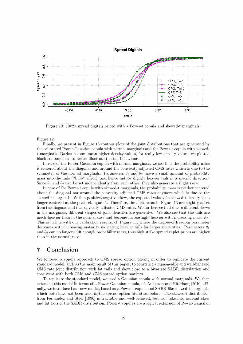
Figure 10: 10y2y spread digitals priced with a Power-t copula and skewed-t marginals.

Figure 12.Finally, we present in Figure 13 contour plots of the joint distributions that are generated by

the calibrated Power-Gaussian copula with normal marginals and the Power-t copula with skewed-t marginals. Darker colours mean higher density values, for really low density values, we plottedblack contour lines to better illustrate the tail behaviour.

In case of the Power-Gaussian copula with normal marginals, we see that the probability massis centered about the diagonal and around the convexity-adjusted CMS rates which is due to thesymmetry of the normal marginals. Parameters θ1 and θ2 move a small amount of probabilitymass into the tails (“bulb” effect), and hence induce slightly heavier tails in a specific direction.Since θ1 and θ2 can be set independently from each other, they also generate a slight skew.

In case of the Power-t copula with skewed-t marginals, the probability mass is neither centeredabout the diagonal nor around the convexity-adjusted CMS rates anymore which is due to theskewed-t marginals. With a positive/negative skew, the expected value of a skewed-t density is nolonger centered at the peak, cf. figure 1. Therefore, the dark areas in Figure 13 are slightly offsetfrom the diagonal and the convexity-adjusted CMS rates. We further see that due to different skewsin the marginals, different shapes of joint densities are generated. We also see that the tails aremuch heavier than in the normal case and become increasingly heavier with increasing maturity.This is in line with our calibration results, cf. Figure 11, where the degree-of freedom parameterdecreases with increasing maturity indicating heavier tails for larger maturities. Parameters θ1and θ2 can no longer shift enough probability mass, thus high strike spread caplet prices are higherthan in the normal case.

7 Conclusion

We followed a copula approach to CMS spread option pricing in order to replicate the currentstandard model, and, as the main result of this paper, to construct a manageable and well-behavedCMS rate joint distribution with fat tails and skew close to a bivariate SABR distribution andconsistent with both CMS and CMS spread option markets.

To replicate the standard model, we used a Gaussian copula with normal marginals. We thenextended this model in terms of a Power-Gaussian copula, cf. Andersen and Piterbarg [2010]. Fi-nally, we introduced our new model, based on a Power-t copula and SABR-like skewed-t marginals,which both have not been used in the spread option literature before. The skewed-t distributionfrom Fernandez and Steel [1996] is tractable and well-behaved, but can take into account skewand fat tails of the SABR distribution. Power-t copulas are a logical extension of Power-Gaussian

19

copulas and rich enough to produce a natural joint distribution with skew and heavy tails, butsimple enough to maintain tractability.

Extensive numerical tests showed that the standard model recovers spread option prices strike-wise very well, but is inconsistent with the CMS cap market and produces distortions in CMSspread digitals.

We further numerically analysed the extended model, ie. the effect of a Power-Gaussian copula.The Power-Gaussian copula smoothed out jumps/kinks present in the correlation skew implied bythe standard model. As a result, CMS spread digital prices were smooth in the extended model,but the inconsistency to the CMS cap market remained (due to the normal marginals).

Finally, we tested our new model. We found that CMS caps, and as a consequence CMSfloors, swaps and SABR swaptions, were accurately recovered (due to the SABR-like skewed-tdistribution). For lower maturities, the CMS spread option market could be recovered as well, forhigher maturities, high strike spread cap prices were too high, indicating a possible inconsistencyin the CMS and CMS spread market.

20

Figure 11: Fits of skewed-t distributions to 10y and 2y CMS digitals.

21

Figure 12: Power-t copula calibrated to 10y2y normal correlations and parameter sensitivities.

22

Figure 13: Joint densities generated by calibrated Power-Gaussian copulas with normal marginalsand Power-t copulas with skewed-t marginals.

23

A Appendix

A.1 Copula Derivatives and Properties

In (0, 1)2, it holds:

∂

∂u1CG(u1, u2) = Φ

(Φ−1(u2)− ρΦ−1(u1)√

1− ρ2

)∂2

∂u1∂u2CG(u1, u2) = ϕ

(Φ−1(u2)− ρΦ−1(u1)√

1− ρ2

)1√

1− ρ2ϕ(Φ−1(u2))

∂

∂u1CT (u1, u2) = Fd+1

(F−1d (u2)− ρF−1d (u1)√

1− ρ2

√d+ 1

d+ F−1d (u1)2

)∂2

∂u1∂u2CT (u1, u2) = fd+1

(F−1d (u2)− ρF−1d (u1)√

1− ρ2

√d+ 1

d+ F−1d (u1)2

)√d+ 1

d+ F−1d (u1)21√

1− ρ2fd(F−1d (u2))

∂

∂u1CP (u1, u2) = u1−θ22

((1− θ1)u−θ11 C(uθ11 , u

θ22 ) + θ1

∂

∂u1C(uθ11 , u

θ22 )

)∂2

∂u1∂u2CP (u1, u2) = (1− θ1)u−θ11 (1− θ2)u−θ22 C(uθ11 , u

θ22 ) + θ1θ2

∂2

∂u1∂u2C(uθ11 , u

θ22 )

+ θ1(1− θ2)u−θ22

∂

∂u1C(uθ11 , u

θ22 ) + θ2(1− θ1)u−θ11

∂

∂u2C(uθ11 , u

θ22 ).

ϕ denotes the standard normal density, fd the Student-t density with d degrees of freedom. Wehave almost everywhere:

C(u1, u2) ∈ [0, 1], nondecreasing

C(u, 0) = C(0, u) = 0

C(u, 1) = C(1, u) = u

∂

∂u1C(u1, u2) ∈ [0, 1], nondecreasing in u2

∂

∂u1C(u1, 0) = 0

∂

∂u1C(u1, 1) = 1.

A.2 Proof of Lemma 5.2

Under the Tp-forward measure, S(T ) has the density fµ,σ,ε,d. We therefore have

ETp [max(S(T )−K, 0)] =

∫ ∞−∞

max(x−K, 0)fµ,σ,ε,d(x)dx

=

∫ ∞K

(x−K)fµ,σ,ε,d(x)dx.

We are now left with two cases. When K < µ:∫ ∞K

(x−K)fµ,σ,ε,d(x)dx =

=2

σ(ε+ 1ε )

(∫ µ

K

(x−K)fd

(ε(x− µ)

σ

)dx+

∫ ∞µ

(x−K)fd

(x− µσε

)dx

)

24

=2

ε+ 1ε

(∫ 0

ε(K−µ)σ

(σ

εx+ µ−K)

fd(x)

εdx+

∫ ∞0

(σεx+ µ−K)εfd(x)dx

)

=2

ε+ 1ε

(σ

ε2

∫ 0

ε(K−µ)σ

xfd(x)dx− K − µε

∫ 0

ε(K−µ)σ

fd(x)dx

+σε2∫ ∞0

xfd(x)dx− ε(K − µ)

∫ ∞0

fd(x)dx

)

=2

ε+ 1ε

(− σε2

d

d− 1fd(0) + σε2

d

d− 1fd(0) +

σ

ε2d+ ε2(K−µ)2

σ2

d− 1fd

(ε(K − µ)

σ

)− K − µ

2

(ε+

1

ε

)+K − µε

Fd

(ε(K − µ)

σ

))= µ+ 2σ

(ε− 1

ε

)d

d− 1fd(0)−K

+2

ε+ 1ε

(σdε2 + (K−µ)2

σ

d− 1fd

(ε(K − µ)

σ

)+K − µε

Fd

(ε(K − µ)

σ

))

where we used that ∫ y

xfd(x)dx = −d+ y2

d− 1fd(y).

This term vanishes at y = ±∞. When K ≥ µ, we similarly get:∫ ∞K

(x−K)fµ,σ,ε,d(x)dx =

=2

σ(ε+ 1ε )

∫ ∞K

(x−K)fd

(x− µσε

)dx

=2

ε+ 1ε

∫ ∞K−µσε

(σεx+ µ−K)εfd(x)dx

=2

ε+ 1ε

(σε2

∫ ∞K−µσε

xfd(x)dx− ε(K − µ)

∫ ∞K−µσε

fd(x)dx

)

=2

ε+ 1ε

(σε2d+ (K−µ)2

σ

d− 1fd

(K − µσε

)− ε(K − µ)

(1− Fd

(K − µσε

))).

The convexity-adjusted CMS rate S(0) can be calculated as a CMS caplet with strike 0.

A.3 Proof of Lemma 5.4

We follow Andersen and Piterbarg [2010]. It holds:

V =

∫ ∞−∞

∫ ∞−∞

max(s1 − s2 −K, 0)ψ(s1, s2)ds1ds2

=

∫ ∞−∞

∫ ∞−∞

(s1 − s2 −K)1ls1−s2−K≥0ψ(s1, s2)ds1ds2

= V1 − V2.

25

Then

V1 =

∫ ∞−∞

∫ ∞−∞

(s1 −K) 1ls1−s2−K≥0ψ(s1, s2)ds1ds2

=

∫ ∞−∞

(s1 −K)ψ1(s1)

∫ ∞−∞

1ls1−s2−K≥0ψ2(s2|s1)ds2ds1

=

∫ ∞−∞

(s1 −K)ψ1(s1)Q(S2(T ) ≤ s1 −K|S1(T ) = s1)ds1

=

∫ ∞−∞

(s1 −K)ψ1(s1)∂

∂u1C(Ψ1(s1),Ψ2(s1 −K)

)ds1

V2 =

∫ ∞−∞

∫ ∞−∞

s21ls1−s2−K≥0ψ(s1, s2)ds1ds2

=

∫ ∞−∞

s2ψ2(s2)

∫ ∞−∞

1ls1−s2−K≥0ψ1(s1|s2)ds1ds2

=

∫ ∞−∞

s2ψ2(s2)(1−Q(S1(T ) ≤ s2 +K|S2(T ) = s2))ds2

=

∫ ∞−∞

s2ψ2(s2)

(1− ∂

∂u2C(Ψ1(s2 +K),Ψ2(s2)

))ds2.

Above, we used the general copula property

Q(U2 ≤ u2|U1 = u1) =∂

∂u1C(u1, u2

)

References

C. Alexander and A. Scourse. Bivariate Normal Mixture Spread Option Valuation. ISMA CentreDiscussion Papers in Finance, 2003.

L.B.G. Andersen and V.V. Piterbarg. Moment Explosions in Stochastic Volatility Models, 2005.URL http://www.ssrn.com. WP.

L.B.G. Andersen and V.V. Piterbarg. Interest Rate Modeling. Atlantic Financial Press, 2010.

P. Austing. Repricing the cross smile: an analytic joint density. Risk, 2011.

E. Benhamou and O. Croissant. Local time for the SABR model, Connection with the complexBlack Scholes And application to CMS and Spread Options, 2007. URL http://www.ssrn.com.

M. Bennett and J. Kennedy. Quanto pricing with copulas. Journal of Derivatives, 2004.

M. Berrahoui. Pricing CMS Spread Options and Digital CMS Spread Options with Smile. WilmottMagazine, 2004.

R. Carmona and V. Durrleman. Pricing and Hedging Spread Options. SIAM Review, 45, No. 4,2003.

U. Cherubini, E. Luciano, and W. Vecchiato. Multivariate Option Pricing With Copulas, 2001.URL http://www.ssrn.com.

U. Cherubini, E. Luciano, and W. Vecchiato. Copula Methods in Finance. Wiley, 2004.

M.A.H. Dempster and S.S.G. Hong. Pricing Spread Options with the Fast Fourier Transform.Risk, 2001.

26

A. Elices and J.P. Fouque. Perturbed Gaussian copula: introducing the skew effect in co-dependence. Risk, 2012.

C. Fernandez and M.F.J. Steel. On Bayesian Modelling of Fat Tails and Skewness, 1996. URLhttp://www.ssrn.com. WP.

P.S. Hagan. Convexity Conundrums: Pricing CMS Swaps, Caps, and Floors, 2003. WilmottMagazine.

P.S. Hagan, D. Kumar, A.S. Lesniewski, and D.E. Woodward. Managing Smile Risk. WilmottMagazine, September, 2002.

P.S. Hagan, A.S. Lesniewski, and D.E. Woodward. Probability Distribution in the SABRModel of Stochastic Volatility, 2005. URL http://lesniewski.us/papers/working/

ProbDistrForSABR.pdf. WP.

P. Henry-Labordre. Analysis, Geometry, and Modeling in Finance. Chapman & Hall, 2008.

B. Jourdain. Loss of Martingality in Asset Price Models with Lognormal Stochastic Volatility,2004. URL http://cermics.enpc.fr/reports/CERMICS-2004/CERMICS-2004-267.pdf. WP.

J. Kienitz. Pricing CMS Spread Options - Copulae and Multi-SABR, 2011. ICBI Global Deriva-tives, Paris.

S. Kotz and S. Nadarajah. Multivariate t Distributions and Their Applications. Cambridge Uni-versity Press, 2004.

E. Liebscher. Construction of asymmetric multivariate copulas. Journal of Multivariate Analysis,99(10), 2008.

P. McCloud. The CMS triangle arbitrage. Risk, 2011.

R.B. Nelsen. An Introduction to Copulas. Springer, 2nd edition, 2006.

V. V. Piterbarg. Spread options, Farkas’s lemma and linear programming. Risk, 2011.

W.T. Shaw and K.T.A. Lee. Copula Methods vs Canonical Multivariate Distributions: themultivariate Student T distribution with general degrees of freedom, 2007. URL http:

//www.defaultrisk.com.

27