Connections fromCorona to Geospace

Markus Aschwanden et al. Lockheed Martin Solar & Astrophysics Laboratory

AIA/HMI Workshop, Monterey – Feb 13-17, 2006 Session C7/M5: Connections to Geospace

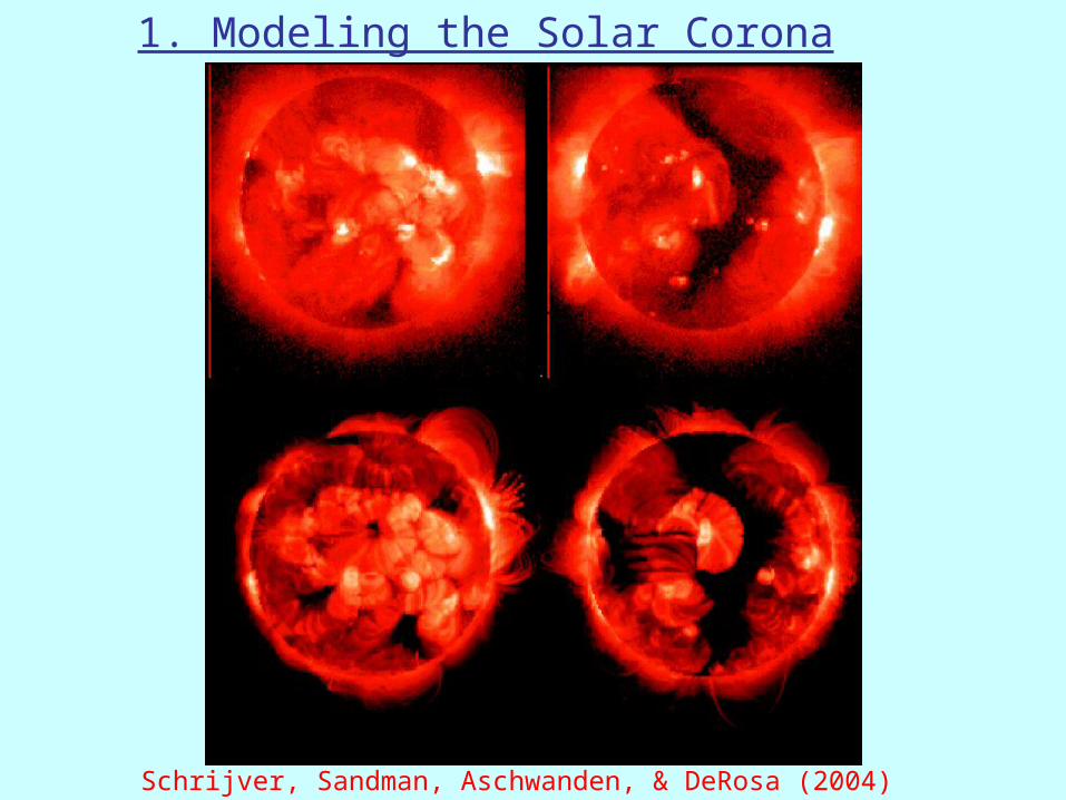
1. Modeling the Solar Corona

Schrijver, Sandman, Aschwanden, & DeRosa (2004)

A full-scale 3D model of the solar corona:(Schrijver et al. 2004)

-3D magnetic field model (using Potential source surface model) computed from synoptic (full-Sun) photospheric magnetogram10^5 loop structures

-Coronal heating function E_H(x,y,z=0)~B(x,y)^a*L(x,y)^b a~1, b~-1

-Hydrostatic loop solutions E_H(s)-E_rad(s)-E_cond(s)=0yield density n_e(s) and T_e(s) profiles

-Line-of-sight integration yields DEM for every image pixel dEM(T,x,y)/ds = Int[ n_e^2(x,y,z,T[x,y,z])] dz

-Free parameters can be varied until synthetic image matches observed ones in each temperature filter

-STEREO will provide double constraint with two independent line-of-sights.

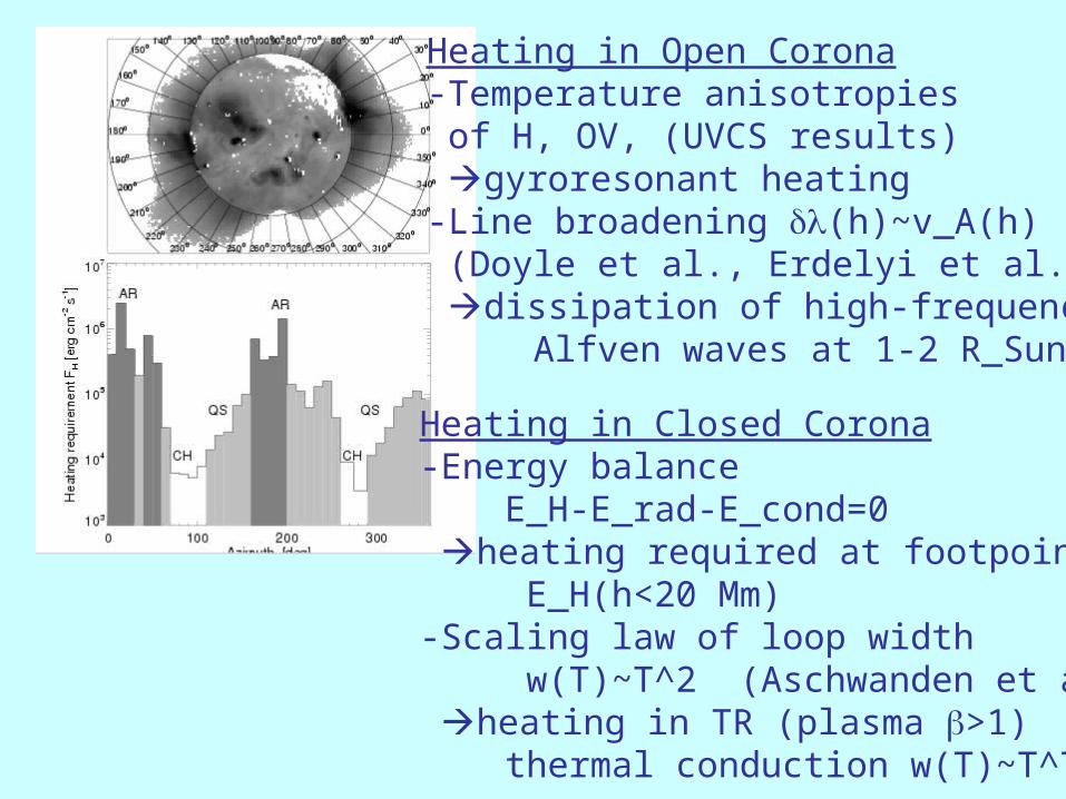
Heating in Open Corona-Temperature anisotropies of H, OV, (UVCS results) gyroresonant heating-Line broadening (h)~v_A(h) (Doyle et al., Erdelyi et al.) dissipation of high-frequency Alfven waves at 1-2 R_Sun

Heating in Closed Corona-Energy balance E_H-E_rad-E_cond=0 heating required at footpoints E_H(h<20 Mm)-Scaling law of loop width w(T)~T^2 (Aschwanden et al.) heating in TR (plasma >1) thermal conduction w(T)~T^7/4

Hydrostatic/hydrodynamic modeling of coronal loopsrequires careful disentangling of neighbored loops,background modeling, multi-component modeling,and multi-filter temperature modeling. Accuratemodeling requires the identification of elementary loops.

Elementary vs. Composite loops:

Each loop strand represents an “isolated mini-atmosphere”and has its own hydrodynamic structure T(s), n_e(s), which needs to be extracted by subtracting it from thebackground coronal structures.SECCHI/EUVI (1.6” pixels) will be able to resolve some individual loops, substantially better than CDS (4” pixels), but somewhat less than TRACE (0.5” pixels).

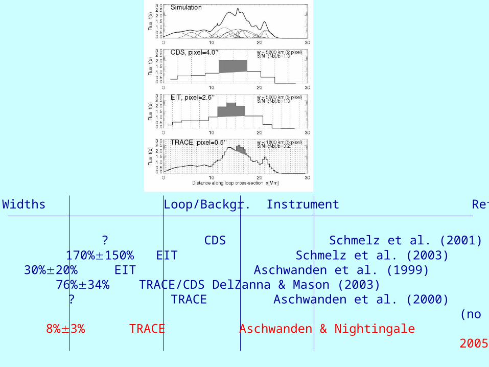
Loops Widths Loop/Backgr. Instrument Ref.

1 ~12 Mm ? CDS Schmelz et al. (2001)10 ? 170%150% EIT Schmelz et al. (2003)30 7.10.8 Mm 30%20% EIT Aschwanden et al. (1999) 1 ~5.8 Mm 76%34% TRACE/CDS DelZanna & Mason (2003)41 3.71.5 Mm ? TRACE Aschwanden et al. (2000) (no highpass filter)234 1.40.2 Mm 8%3% TRACE Aschwanden & Nightingale 2005 (with highpass filter)

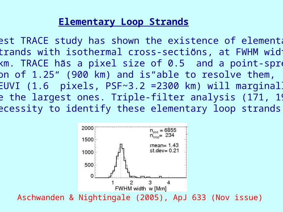
Elementary Loop Strands

The latest TRACE study has shown the existence of elementary loop strands with isothermal cross-sections, at FWHM widths of <2000 km. TRACE has a pixel size of 0.5” and a point-spread function of 1.25” (900 km) and is able to resolve them, while EUVI (1.6” pixels, PSF~3.2”=2300 km) will marginally resolve the largest ones. Triple-filter analysis (171, 195, 284) is a necessity to identify these elementary loop strands.

Aschwanden & Nightingale (2005), ApJ 633 (Nov issue)

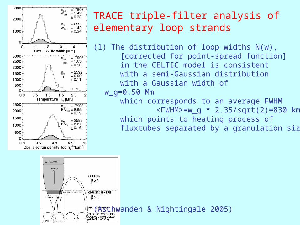
TRACE triple-filter analysis ofelementary loop strands

(1) The distribution of loop widths N(w), [corrected for point-spread function] in the CELTIC model is consistent with a semi-Gaussian distribution with a Gaussian width of

w_g=0.50 Mm which corresponds to an average FWHM <FWHM>=w_g * 2.35/sqrt(2)=830 km which points to heating process of fluxtubes separated by a granulation size.

(Aschwanden & Nightingale 2005)

Scaling law of width with temperaturein elementary loop strands

Observational result from TRACETriple-filter data analysis of elementaryloop strands (with isothermal cross-sections):

97.1)( TTw

2

2/72/7

L

T

s

T

sFE cH

75.14/7)( TTTw

Loop widths cannot adjust to temperature incorona because plasma- << 1, and thuscross-section w is formed in TR at >1Thermal conduction across loop widthsIn TR predicts scaling law:

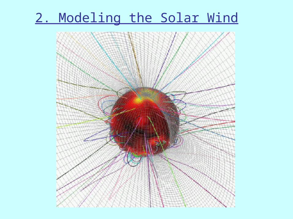
2. Modeling the Solar Wind

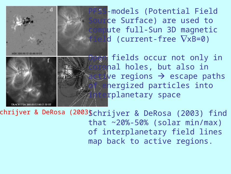
Schrijver & DeRosa (2003)

PFSS-models (Potential FieldSource Surface) are used tocompute full-Sun 3D magneticfield (current-free xB=0)

Open fields occur not only incoronal holes, but also inactive regions escape pathsof energized particles intointerplanetary space

Schrijver & DeRosa (2003) findthat ~20%-50% (solar min/max)of interplanetary field linesmap back to active regions.

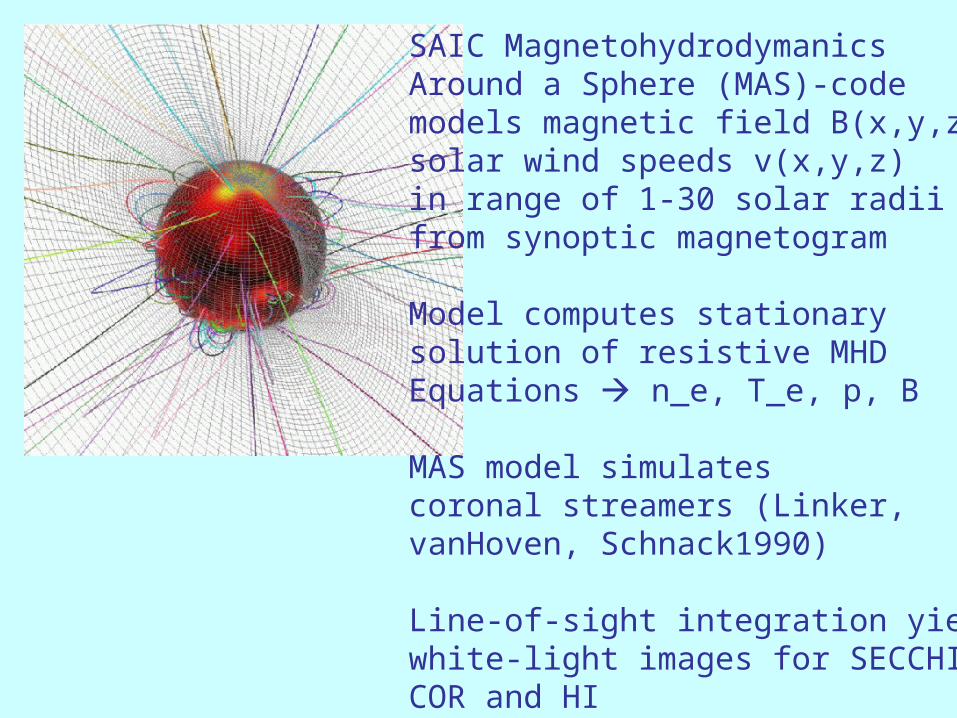
SAIC MagnetohydrodymanicsAround a Sphere (MAS)-codemodels magnetic field B(x,y,z)solar wind speeds v(x,y,z)in range of 1-30 solar radiifrom synoptic magnetogram

Model computes stationarysolution of resistive MHDEquations n_e, T_e, p, B

MAS model simulatescoronal streamers (Linker, vanHoven, Schnack1990)

Line-of-sight integration yieldswhite-light images for SECCHI/COR and HI

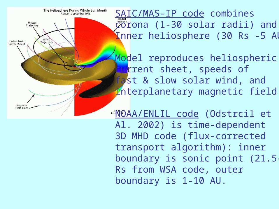
SAIC/MAS-IP code combinescorona (1-30 solar radii) andInner heliosphere (30 Rs -5 AU)

Model reproduces heliosphericcurrent sheet, speeds offast & slow solar wind, and interplanetary magnetic field

NOAA/ENLIL code (Odstrcil etAl. 2002) is time-dependent3D MHD code (flux-correctedtransport algorithm): innerboundary is sonic point (21.5-30 Rs from WSA code, outerboundary is 1-10 AU.

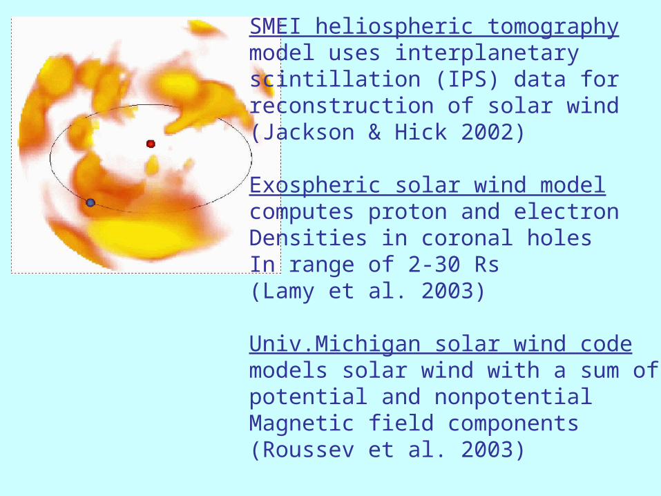
SMEI heliospheric tomographymodel uses interplanetaryscintillation (IPS) data forreconstruction of solar wind(Jackson & Hick 2002)

Exospheric solar wind modelcomputes proton and electronDensities in coronal holesIn range of 2-30 Rs(Lamy et al. 2003)

Univ.Michigan solar wind codemodels solar wind with a sum ofpotential and nonpotentialMagnetic field components(Roussev et al. 2003)

3. Modeling of Erupting Filaments

Roussev et al. (2003)

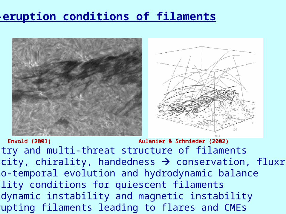
Pre-eruption conditions of filaments

-Geometry and multi-threat structure of filaments (helicity, chirality, handedness conservation, fluxropes)-Spatio-temporal evolution and hydrodynamic balance-Stability conditions for quiescent filaments-Hydrodynamic instability and magnetic instability of erupting filaments leading to flares and CMEs

Envold (2001)Envold (2001) Aulanier & Schmieder (2002)Aulanier & Schmieder (2002)

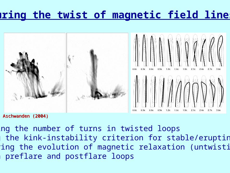
Measuring the twist of magnetic field lines

Aschwanden (2004)Aschwanden (2004)

-Measuring the number of turns in twisted loops-Testing the kink-instability criterion for stable/erupting loops-Monitoring the evolution of magnetic relaxation (untwisting) between preflare and postflare loops

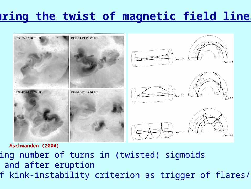
Measuring the twist of magnetic field lines

Aschwanden (2004)Aschwanden (2004)

-Measuring number of turns in (twisted) sigmoids before and after eruption-Test of kink-instability criterion as trigger of flares/CMEs

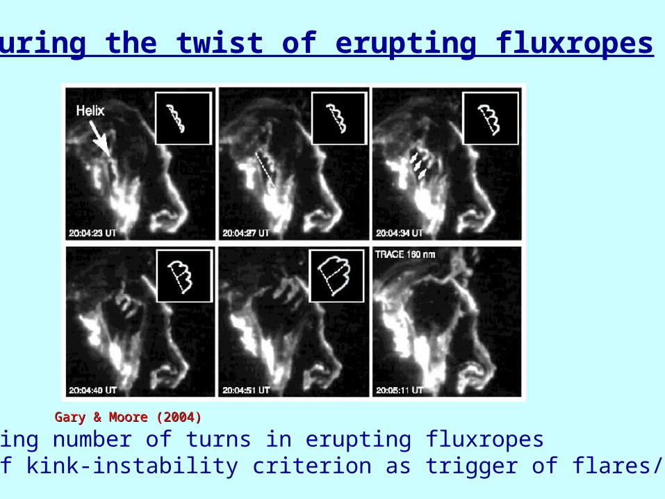
Measuring the twist of erupting fluxropes

Gary & Moore (2004)Gary & Moore (2004)

-Measuring number of turns in erupting fluxropes-Test of kink-instability criterion as trigger of flares/CMEs

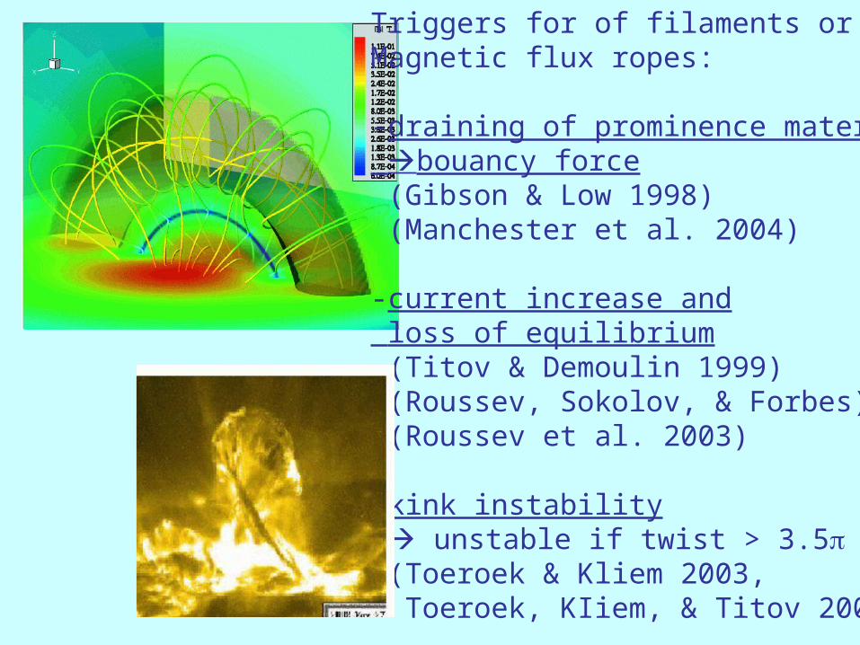
Triggers for of filaments orMagnetic flux ropes:

-draining of prominence material bouancy force (Gibson & Low 1998) (Manchester et al. 2004)

-current increase and loss of equilibrium (Titov & Demoulin 1999) (Roussev, Sokolov, & Forbes) (Roussev et al. 2003)

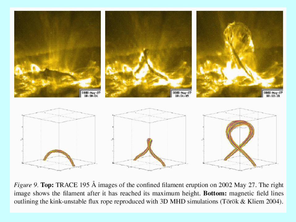
-kink instability unstable if twist > 3.5 (Toeroek & Kliem 2003, Toeroek, KIiem, & Titov 2003)

Roussev et al. (2004)

MHD simulations of coronal dimming:-evacuation of plasma beneath CME, fast-mode MHD wave (Wang 2000; Chen et al. 2002; Wu et al. 2001)

5. Modeling of Coronal Mass Ejections (CMEs)

MAS/ENLIL code streamer, eruption and evolution of CME(Mikic & Linker 1994; Lionello et al. 1998; Mikic et al. 1999)Linker et al. 1999)

pB

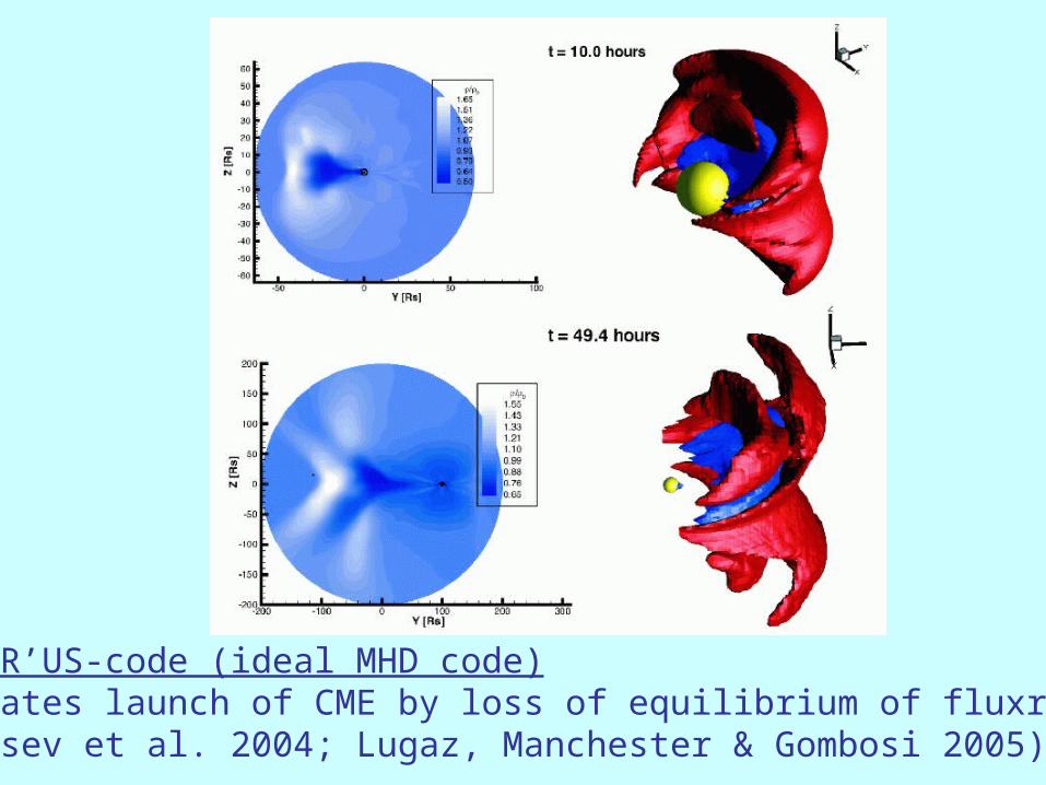
BATS`R’US-code (ideal MHD code) Simulates launch of CME by loss of equilibrium of fluxrope(Roussev et al. 2004; Lugaz, Manchester & Gombosi 2005)

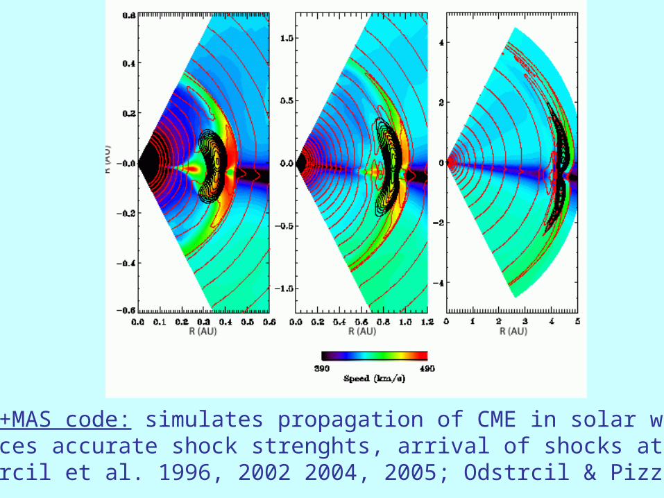
ENLIL+MAS code: simulates propagation of CME in solar wind,produces accurate shock strenghts, arrival of shocks at 1 AU(Odstrcil et al. 1996, 2002 2004, 2005; Odstrcil & Pizzo 1999)

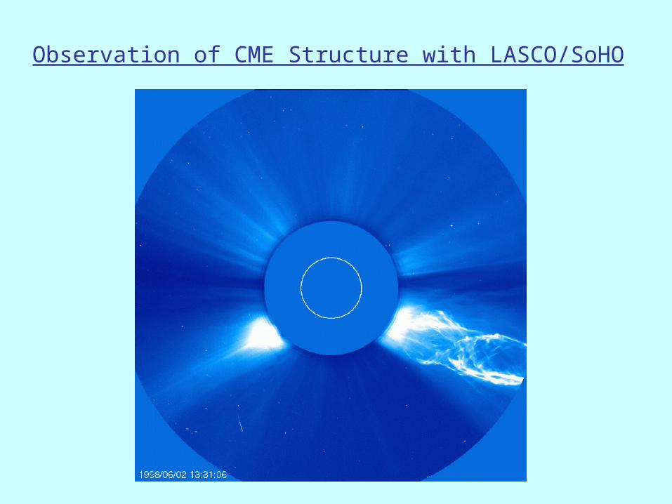
Observation of CME Structure with LASCO/SoHO

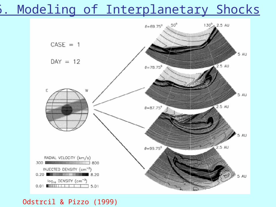
6. Modeling of Interplanetary Shocks

Odstrcil & Pizzo (1999)

Odstrcil & Pizzo (1999)

Fast CMEs have speeds of v>2000 km/sformation of fast-mode shockNumerical MHD simulations: - Mikic & Linker (1994) - Odstrcil & Pizzo (1999) - Odstrcil, Pizzo, & Arge (2005)

Predicted arrival time at 1 AU dependscritically on models of backgroundsolar wind which controls shockpropagation speed - Odstrcil, Pizzo & Arge (2005)

CME cannibalism (faster overtakesslower one) compound streams,interactions with CIR (corotatinginteraction regions) controlshock-accelerated particles (SEPs)

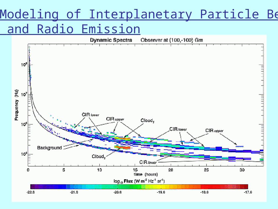
7. Modeling of Interplanetary Particle Beams and Radio Emission

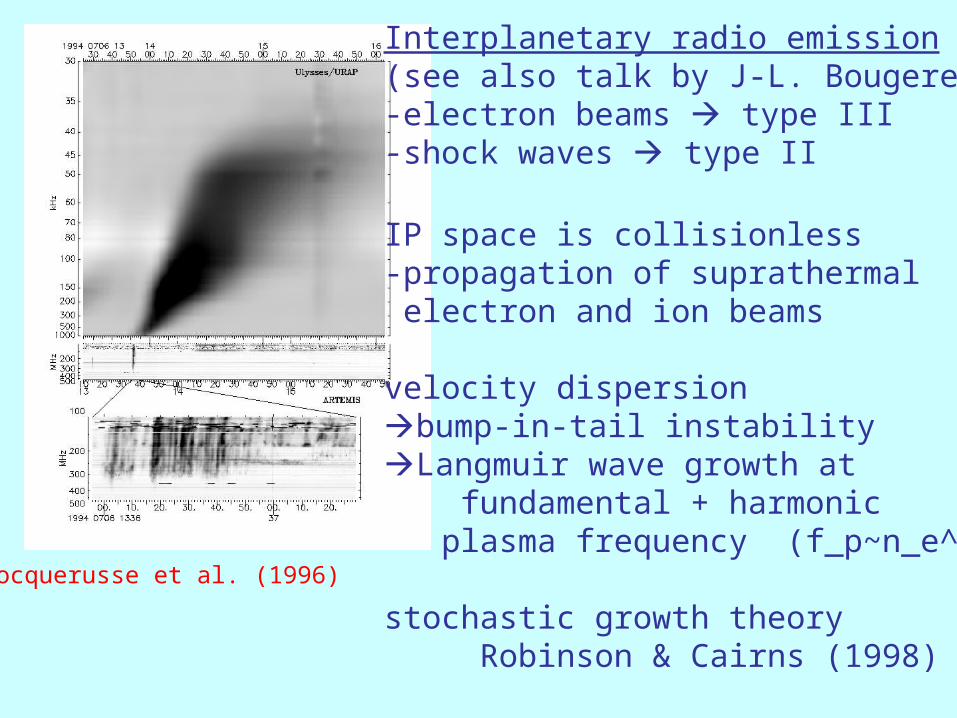
Pocquerusse et al. (1996)

Interplanetary radio emission(see also talk by J-L. Bougeret)-electron beams type III-shock waves type II

IP space is collisionless-propagation of suprathermal electron and ion beams

velocity dispersion bump-in-tail instabilityLangmuir wave growth at fundamental + harmonic plasma frequency (f_p~n_e^1/2)

stochastic growth theory Robinson & Cairns (1998)

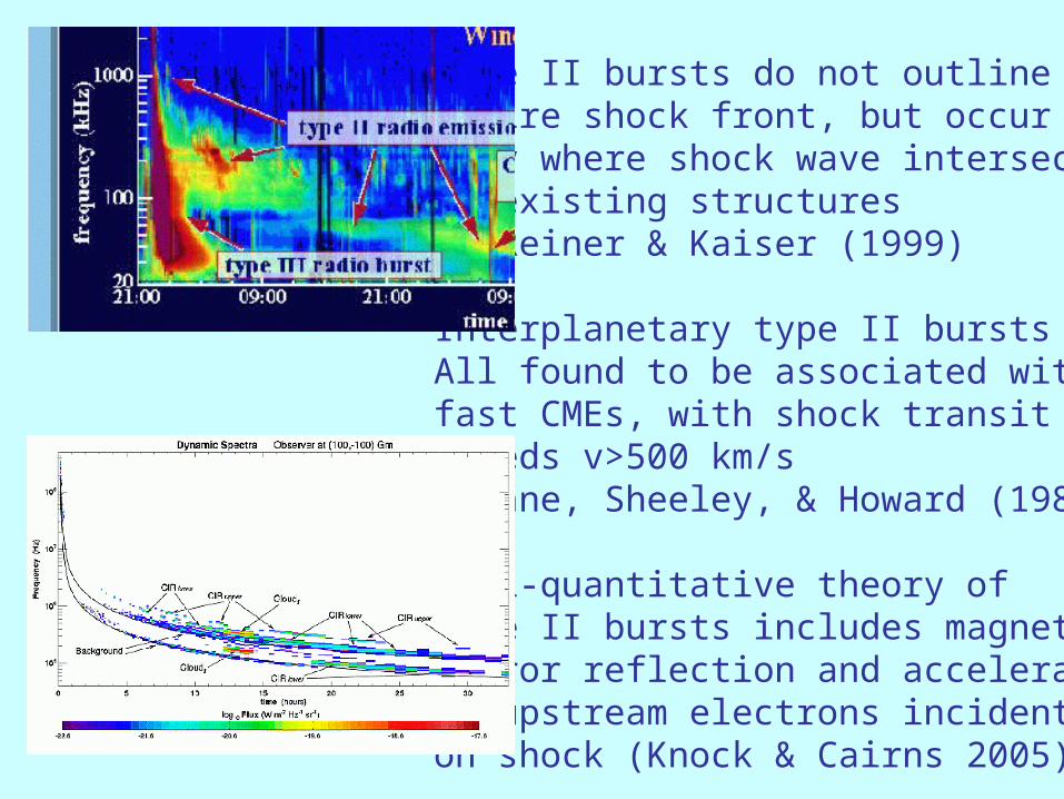
Type II bursts do not outlineentire shock front, but occuronly where shock wave intersectspreexisting structures Reiner & Kaiser (1999)

Interplanetary type II bursts wereAll found to be associated withfast CMEs, with shock transitSpeeds v>500 km/s Cane, Sheeley, & Howard (1987)

Semi-quantitative theory oftype II bursts includes magneticmirror reflection and accelerationof upstream electrons incidenton shock (Knock & Cairns 2005)

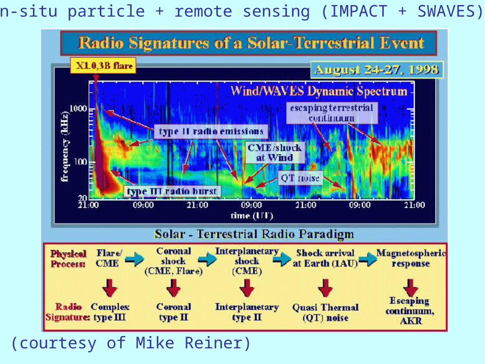
(courtesy of Mike Reiner)

In-situ particle + remote sensing (IMPACT + SWAVES)

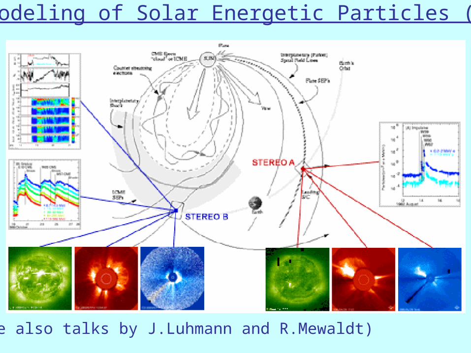
8. Modeling of Solar Energetic Particles (SEPs)

(see also talks by J.Luhmann and R.Mewaldt)

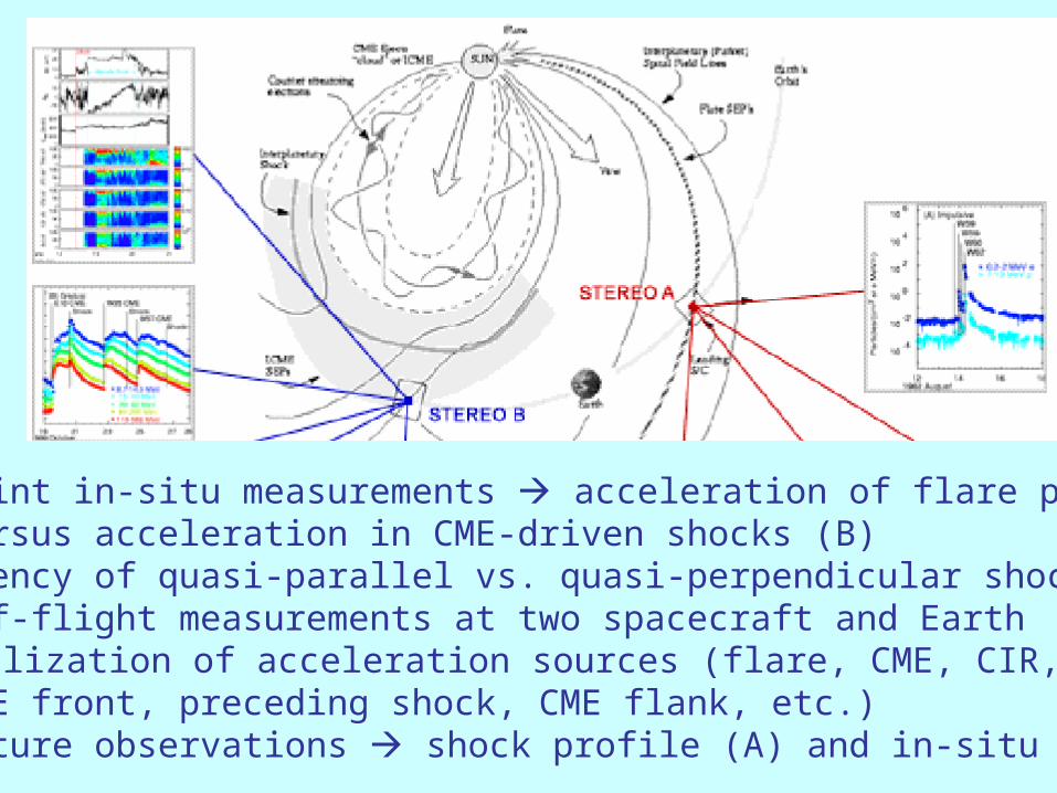
-Two-point in-situ measurements acceleration of flare particles (A) versus acceleration in CME-driven shocks (B)-Efficiency of quasi-parallel vs. quasi-perpendicular shock acc.-Time-of-flight measurements at two spacecraft and Earth localization of acceleration sources (flare, CME, CIR, CME front, preceding shock, CME flank, etc.)-Quadrature observations shock profile (A) and in-situ (B)

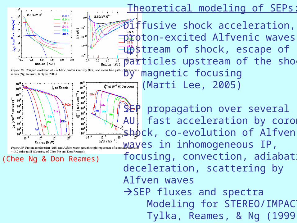
(Chee Ng & Don Reames)

Theoretical modeling of SEPs:

Diffusive shock acceleration,proton-excited Alfvenic wavesupstream of shock, escape ofparticles upstream of the shockby magnetic focusing (Marti Lee, 2005)

SEP propagation over severalAU, fast acceleration by coronalshock, co-evolution of Alfvenwaves in inhomogeneous IP,focusing, convection, adiabaticdeceleration, scattering byAlfven waves SEP fluxes and spectra Modeling for STEREO/IMPACT Tylka, Reames, & Ng (1999)

9. Modeling of Geo-effective events and Space Weather

-Arrival time of shocks at Earth will be improved by 3D triangulation of CME propagation with two spacecraft (STEREO 3D v-vector and r-vector reconstruction vs. LASCO CME speed (lower limit) projected in plane of sky

-End-to-end models attempted including MHD of lower corona, heliosphere, and magnetosphere + SEP accel. & propagation - CCMC (Community Coordinated Modelin Center, GSFC) - CISM (Center for Integrated Space Weather Modeling, UCB) - CSEM (Center for Space Environment Modeling, UMich) - Solar/Muri (Solar Multidisciplinary Univ. Research Initiative)

CONCLUSIONS-The long-term goal is to create end-to-end models that connect the origin and evolution of phenomena from the corona, through heliosphere, to geospace.

Modeling includes background plasma in corona, heliosphere, and solar wind, dynamic phenomena associated with initiation of CMEs in lower corona (filament dynamics, shearing, kinking, loss-of-equilibrium, filament eruption, magnetic reconnection in coronal flare sites), and propagation and evolution of CMEs in interplanetary space (interplanetary shocks, IP particle beams, SEP acceleration and propagation, geoeffective events, space weather).