Conception de Réseaux Dynamiques Tolérants aux Pannes
357
HAL Id: tel-00472781 https://tel.archives-ouvertes.fr/tel-00472781 Submitted on 13 Apr 2010 HAL is a multi-disciplinary open access archive for the deposit and dissemination of sci- entific research documents, whether they are pub- lished or not. The documents may come from teaching and research institutions in France or abroad, or from public or private research centers. L’archive ouverte pluridisciplinaire HAL, est destinée au dépôt et à la diffusion de documents scientifiques de niveau recherche, publiés ou non, émanant des établissements d’enseignement et de recherche français ou étrangers, des laboratoires publics ou privés. Conception de Réseaux Dynamiques Tolérants aux Pannes Florian Huc To cite this version: Florian Huc. Conception de Réseaux Dynamiques Tolérants aux Pannes. Réseaux et télécommunica- tions [cs.NI]. Université Nice Sophia Antipolis, 2008. Français. tel-00472781
Transcript of Conception de Réseaux Dynamiques Tolérants aux Pannes
HAL Id: tel-00472781https://tel.archives-ouvertes.fr/tel-00472781
Submitted on 13 Apr 2010
HAL is a multi-disciplinary open accessarchive for the deposit and dissemination of sci-entific research documents, whether they are pub-lished or not. The documents may come fromteaching and research institutions in France orabroad, or from public or private research centers.
L’archive ouverte pluridisciplinaire HAL, estdestinée au dépôt et à la diffusion de documentsscientifiques de niveau recherche, publiés ou non,émanant des établissements d’enseignement et derecherche français ou étrangers, des laboratoirespublics ou privés.
Conception de Réseaux Dynamiques Tolérants auxPannes
Florian Huc
To cite this version:Florian Huc. Conception de Réseaux Dynamiques Tolérants aux Pannes. Réseaux et télécommunica-tions [cs.NI]. Université Nice Sophia Antipolis, 2008. Français. tel-00472781
No d’ordre: 00000
THESE
Présentée devant
devant l’Université de Nice Sophia Antipolis
pour obtenir
le grade de : Docteur de l’Université de Nice Sophia AntipolisMention Informatique
par
Florian Huc
Equipe d’accueil : Projet MASCOTTEEcole Doctorale : ED-STIC
Composante universitaire : I3S (CNRS - UNSA) INRIA
Titre de la thèse :Conception de Réseaux Dynamiques Tolérants aux Pannes
soutenue le 14 novembre 2008 devant la commission d’examen
M. : Jean-Claude König PrésidentMM. : Pierre Fraigniaud Rapporteurs
Arie KosterAndrew Thomason
MM. : David Coudert ExaminateursJean-Claude KönigYann VaxèsJean-Claude Bermond


Remerciements
Je tiens à remercier tout particulièrement Jean-Claude Bermond qui a été mondirecteur de thèse ainsi que David mon (presque, à une signature près) co-directeur dethèse. Toutes les discussions que nous avons eues m’ont beaucoup appris, et vos conseilsm’ont été et me seront encore très utiles. Merci aussi pour toutes les opportunités quevous m’avez ouvertes et amenées à saisir au cours de ces trois ans.
Merci également à Pierre Fraigniaud, Arie Koster et Andrew Thomasson pour avoirété rapporteurs de ma thèse, ainsi qu’a Jean-Claude König et Yann Vaxès pour avoirparticipé à mon jury.
Merci Patricia Lachaume, Ephie Dériche et Sandra Devauchelle pour votre gen-tillesse et votre aide si précieuse pour venir à bout de tous les papiers administratifs.
Un grand merci à tous les membres du projet MASCOTTE, notamment à Jean-Claude sans qui MASCOTTE serait tout autre et qui aura réussi à me faire courir unmarathon relais avec une équipe formidable. Merci à David qui m’a permis d’agrandirma collection de guides du routard et de lonely planet, à Frédéric & Frédéric pour lesfranches rigolades et les barbecues, à Joanna pour ses conseils et sa bonne humeur, àStéphane pour ses idées, à Bruce pour le meilleur whisky que j’ai jamais bu et les bonsmoments passés, à Hervé pour ses nombreux conseils et sa disponibilité, à Michel et àl’IUT pour toutes leurs histoires. Merci également à tous les sud-américains Cristiana,Juan-Carlos, Julian, Napoleao et Patricio pour leur aide précieuse pour faire de lacaipirinha et leur gentillesse. Merci aussi à Marie avec qui, à mon grand regret, jen’aurais pas eu assez de temps pour faire de l’escalade, à Nathann et sa curiositéinsatiable qui m’auront fait découvrir de nombreuses choses, à Christelle et à sa tortueCacahuète dont j’aurais tant entendu parlé, à Dorian avec qui ça a été un plaisir detravailler et qui, j’en suis désolé, a hérité d’un surnom par ma faute (mais aussi celled’Hervé tout de même), à Judicael et aussi à Ignasi avec qui ce fut un plaisir de travailleret de voyager. Merci aussi à Marie-Emilie, Jean-Sébastien et Omid, qui ont été dansMASCOTTE mais qui en sont parti avant que je ne finisse ma thèse. Merci à touspour la bonne ambiance qui règne au sein de l’équipe, rendant agréable le fait de venirtravailler.
Merci à ma famille bien sur et à toutes ses "pièces rapportées", cela va de soi, mercid’être là. Merci à Héloïse pour les bons moments passés ensemble et tous ceux à venir.
Merci à Omid, Pooran, Alexandre et Guillaume pour avoir passé tant de temps encolloc ensemble et être devenu ma famille Antiboise.
Merci à Nicolas et Yoann pour leur amitié exceptionnelle, les fou-rires, les bataillesacharnées, leur complicité et leur présence tout simplement. Merci à Xavier pour sonamitié.
Merci à Yvan, Marie, Annelise (sans y) et Aurélie que la distance n’a pas éloignés.Merci à tous mes amis de Cahors, Guillaume, Bertrand, Delphine, Virginie, Pierre
et Adeline qui sont tout aussi indispensables.Merci à Pierre, Sylvain, Sapna, Vincent, Benjamin, Nicolas, Nathalia, Damien, De-
mian, Nadia, Senem, Ozge, Pinar ... et tous les autres sans lesquels la vie ici n’auraitpas été pareille.

6
Merci à tous ceux que j’ai rencontrés pendant mes déplacements, avant ou pendantma thèse, Simon, Nicolas et Olga tout particulièrement mais aussi Frederico, Luis,Louis, Yusuf, Brigitte et tous les autres.
Table des matières
1 Introduction 111.1 Principaux résultats obtenus . . . . . . . . . . . . . . . . . . . . . . . . 121.2 Réseaux de télécommunication : problématiques et techniques . . . . . . 161.3 Publications . . . . . . . . . . . . . . . . . . . . . . . . . . . . . . . . . . 17
2 Notions de base 192.1 Définitions et notations . . . . . . . . . . . . . . . . . . . . . . . . . . . 19
2.1.1 Graphes . . . . . . . . . . . . . . . . . . . . . . . . . . . . . . . . 192.1.2 Caractéristiques des graphes . . . . . . . . . . . . . . . . . . . . 202.1.3 Quelques familles de graphes . . . . . . . . . . . . . . . . . . . . 20
2.2 Introduction sur les réseaux . . . . . . . . . . . . . . . . . . . . . . . . . 222.2.1 Fonctionnement général d’un réseau, le modèle OSI, Open Sys-
tems Interconnection . . . . . . . . . . . . . . . . . . . . . . . . . 222.2.2 Rappels sur le multiflot classique . . . . . . . . . . . . . . . . . . 23
3 Conception de réseaux tolérants aux pannes 273.1 Concentrateurs, superconcentrateurs et graphes d’expansion . . . . . . . 293.2 Réseaux (p,λ,k) . . . . . . . . . . . . . . . . . . . . . . . . . . . . . . . . 303.3 Résultats antérieurs . . . . . . . . . . . . . . . . . . . . . . . . . . . . . 333.4 Réseaux tolérant un grand nombre de pannes : contributions . . . . . . 34
3.4.1 Robustesse des graphes 4-réguliers . . . . . . . . . . . . . . . . . 383.5 Conclusion et perspectives . . . . . . . . . . . . . . . . . . . . . . . . . . 38
4 Algorithmes de routage 414.1 Algorithmes de routage dans les grilles . . . . . . . . . . . . . . . . . . . 42
4.1.1 Contexte . . . . . . . . . . . . . . . . . . . . . . . . . . . . . . . 424.1.2 Les différents scénarios de requêtes . . . . . . . . . . . . . . . . . 434.1.3 Les différents types de réseaux . . . . . . . . . . . . . . . . . . . 434.1.4 Résultats connus dans la grille carrée . . . . . . . . . . . . . . . . 444.1.5 Algorithmes de routage dans les grilles hexagonales et triangu-
laires : contributions . . . . . . . . . . . . . . . . . . . . . . . . . 454.2 Allocation de fréquences et coloration impropre des graphes hexagonaux
pondérés . . . . . . . . . . . . . . . . . . . . . . . . . . . . . . . . . . . . 464.2.1 Origine du problème . . . . . . . . . . . . . . . . . . . . . . . . . 46
7

8 Table des matières
4.2.2 Algorithmes d’approximation . . . . . . . . . . . . . . . . . . . . 484.3 Optimisation des buffers dans les réseaux radios et coloration propor-
tionnelle . . . . . . . . . . . . . . . . . . . . . . . . . . . . . . . . . . . . 504.3.1 Origine du problème . . . . . . . . . . . . . . . . . . . . . . . . . 504.3.2 Complexité . . . . . . . . . . . . . . . . . . . . . . . . . . . . . . 53
4.4 Conclusion et Perspectives . . . . . . . . . . . . . . . . . . . . . . . . . . 54
5 Réseaux d’accès et de cœur 555.1 Introduction sur les réseaux optiques . . . . . . . . . . . . . . . . . . . . 56
5.1.1 Technologies optiques . . . . . . . . . . . . . . . . . . . . . . . . 565.1.1.1 Fibres optiques . . . . . . . . . . . . . . . . . . . . . . . 565.1.1.2 Émetteurs . . . . . . . . . . . . . . . . . . . . . . . . . 575.1.1.3 Récepteurs . . . . . . . . . . . . . . . . . . . . . . . . . 585.1.1.4 Amplificateurs . . . . . . . . . . . . . . . . . . . . . . . 585.1.1.5 Multiplexage . . . . . . . . . . . . . . . . . . . . . . . . 595.1.1.6 Splitters . . . . . . . . . . . . . . . . . . . . . . . . . . . 60
5.1.2 Modélisation d’un réseau optique WDM . . . . . . . . . . . . . . 615.2 Multicast . . . . . . . . . . . . . . . . . . . . . . . . . . . . . . . . . . . 62
5.2.1 Dimensionnement d’un réseau en étoile . . . . . . . . . . . . . . 635.2.1.1 Une fibre, un multicast . . . . . . . . . . . . . . . . . . 645.2.1.2 Plusieurs fibres, plusieurs multicasts . . . . . . . . . . . 695.2.1.3 Apport d’un splitter . . . . . . . . . . . . . . . . . . . . 71
5.2.2 Multicast dans les réseaux de cœur . . . . . . . . . . . . . . . . . 725.2.3 Entrées des problèmes MC-RWA . . . . . . . . . . . . . . . . . . 745.2.4 Le problème FR-MC-RWA . . . . . . . . . . . . . . . . . . . . . 74
5.2.4.1 Principe de la génération de colonnes . . . . . . . . . . 755.2.4.2 Problème FR-MC-RWA : formulation avec configura-
tion de routage . . . . . . . . . . . . . . . . . . . . . . . 755.2.4.3 Problème FR-MC-RWA : formulation par arbres de rou-
tage . . . . . . . . . . . . . . . . . . . . . . . . . . . . . 785.2.5 Problème PR-MC-RWA . . . . . . . . . . . . . . . . . . . . . . . 80
5.2.5.1 Problème PR-MC-RWA : formulation avec configura-tion de routage . . . . . . . . . . . . . . . . . . . . . . . 80
5.2.6 Réseaux d’accès . . . . . . . . . . . . . . . . . . . . . . . . . . . . 825.2.6.1 Réseaux Passifs Optiques . . . . . . . . . . . . . . . . . 825.2.6.2 Structure des réseaux PON . . . . . . . . . . . . . . . . 835.2.6.3 Modèles . . . . . . . . . . . . . . . . . . . . . . . . . . . 85
5.3 Conclusion et Perspectives . . . . . . . . . . . . . . . . . . . . . . . . . . 85
6 Fiabilité et tolérance aux pannes 876.1 Réseaux colorés . . . . . . . . . . . . . . . . . . . . . . . . . . . . . . . . 87
6.1.1 Origine du problème . . . . . . . . . . . . . . . . . . . . . . . . . 886.1.2 Notations . . . . . . . . . . . . . . . . . . . . . . . . . . . . . . . 906.1.3 Problème et complexité . . . . . . . . . . . . . . . . . . . . . . . 90

Table des matières 9
6.1.4 Formulations . . . . . . . . . . . . . . . . . . . . . . . . . . . . . 916.1.4.1 Formulation sommet-arc . . . . . . . . . . . . . . . . . 916.1.4.2 Formulation arc-chemin . . . . . . . . . . . . . . . . . . 926.1.4.3 La génération de colonnes appliquée à MACF . . . . . . 92
6.1.5 Résultats expérimentaux . . . . . . . . . . . . . . . . . . . . . . . 936.1.5.1 Génération des instances . . . . . . . . . . . . . . . . . 936.1.5.2 Résultats . . . . . . . . . . . . . . . . . . . . . . . . . . 94
6.1.6 Perspectives . . . . . . . . . . . . . . . . . . . . . . . . . . . . . . 956.2 Protection par segments . . . . . . . . . . . . . . . . . . . . . . . . . . . 96
6.2.1 Contexte . . . . . . . . . . . . . . . . . . . . . . . . . . . . . . . 966.2.2 Protection par segments partagés . . . . . . . . . . . . . . . . . . 97
6.2.2.1 Protection par segments partagés de base . . . . . . . . 986.2.2.2 Protection par segments partagés avec overlaps . . . . . 986.2.2.3 Comparaison des deux modes de protection . . . . . . . 98
6.2.3 Formulations mathématiques . . . . . . . . . . . . . . . . . . . . 1006.3 Conclusion et Perspectives . . . . . . . . . . . . . . . . . . . . . . . . . . 101
7 Reroutage de connexions et Pathwidth 1037.1 Origine du problème . . . . . . . . . . . . . . . . . . . . . . . . . . . . . 1037.2 État de l’art . . . . . . . . . . . . . . . . . . . . . . . . . . . . . . . . . . 106
7.2.1 Process number . . . . . . . . . . . . . . . . . . . . . . . . . . . . 1067.2.2 Vertex separation . . . . . . . . . . . . . . . . . . . . . . . . . . . 1077.2.3 Pathwidth . . . . . . . . . . . . . . . . . . . . . . . . . . . . . . . 1087.2.4 Indice d’échappement sommet . . . . . . . . . . . . . . . . . . . 1087.2.5 Indice d’échappement arête . . . . . . . . . . . . . . . . . . . . . 1107.2.6 Indice d’échappement arête connexe . . . . . . . . . . . . . . . . 111
7.3 Contributions . . . . . . . . . . . . . . . . . . . . . . . . . . . . . . . . . 1127.3.1 Process number d’un arbre . . . . . . . . . . . . . . . . . . . . . 1127.3.2 Pathwidth des graphes planaires extérieurs . . . . . . . . . . . . 1207.3.3 Pathwidth des graphes planaires . . . . . . . . . . . . . . . . . . 1227.3.4 A propos de l’indice d’échappement arête connexe d’un arbre . . 123
7.3.4.1 Arbres pondérés et arbres de cliques . . . . . . . . . . . 1237.3.4.2 Borne inférieure sur la complexité . . . . . . . . . . . . 1257.3.4.3 Version dynamique de l’indice d’échappement arête connexe
non pondéré . . . . . . . . . . . . . . . . . . . . . . . . 1267.4 Conclusion et Perspectives . . . . . . . . . . . . . . . . . . . . . . . . . . 126
8 Conclusion 129
A Conception de réseaux tolérants aux pannes 133A.1 Minimal Selectors and Fault Tolerant Networks . . . . . . . . . . . . . . 133

10 Table des matières
B Algorithmes de routage 164B.1 (ℓ,k)-Routing on Plane Grids . . . . . . . . . . . . . . . . . . . . . . . . 164B.2 On Multiple Improper Colorings . . . . . . . . . . . . . . . . . . . . . . 200B.3 The Proportional Colouring Problem : Optimising Buffers in Radio Mesh
Networks . . . . . . . . . . . . . . . . . . . . . . . . . . . . . . . . . . . 216
C Réseaux d’accès et de cœur 229C.1 WDM and Directed Star Arboricity . . . . . . . . . . . . . . . . . . . . 230C.2 Muticast Routing and Wavelength Assignment in Passive Optical Access
Networks . . . . . . . . . . . . . . . . . . . . . . . . . . . . . . . . . . . 248
D Fiabilité et tolérance aux pannes 259D.1 Reliability of Connections in Multilayer Networks under Shared Risk
Groups and Costs Constraints . . . . . . . . . . . . . . . . . . . . . . . . 260D.2 Overlapping Segment for an Efficient Protection of WDM Networks . . 265
E Reroutage de connexions et Pathwidth 275E.1 A distributed algorithm for computing and updating the process number
of a forest . . . . . . . . . . . . . . . . . . . . . . . . . . . . . . . . . . . 276E.2 Pathwidth of Outerplanar Graphs . . . . . . . . . . . . . . . . . . . . . 295E.3 On the Pathwidth of Planar Graphs . . . . . . . . . . . . . . . . . . . . 308
F Mixing Digraphs 315F.1 On the value of mex(n,e,
−→C ) . . . . . . . . . . . . . . . . . . . . . . . . . 320
F.1.1 A lower bound for mex(n,e,−→C4) . . . . . . . . . . . . . . . . . . . 320
F.1.2 Upper bounds for some mex(n,e,−→C2k) . . . . . . . . . . . . . . . . 324
F.1.3 Simple graphs with no 4-cycles . . . . . . . . . . . . . . . . . . . 324F.1.3.1 First examples . . . . . . . . . . . . . . . . . . . . . . . 324F.1.3.2 Blow-ups . . . . . . . . . . . . . . . . . . . . . . . . . . 324F.1.3.3 The Class of examples . . . . . . . . . . . . . . . . . . . 326
F.1.4 Bounds for mex(n,e,−→C2k) . . . . . . . . . . . . . . . . . . . . . . . 327
F.2 On the value of mex(n,e,H) in dense digraphs . . . . . . . . . . . . . . . 331F.3 maxAB
D . . . . . . . . . . . . . . . . . . . . . . . . . . . . . . . . . . . . . 335F.3.1 Definition and complexity result . . . . . . . . . . . . . . . . . . 335F.3.2 Lower bounds on maxAB
D . . . . . . . . . . . . . . . . . . . . . . . 336F.4 Conclusion and Remaining questions . . . . . . . . . . . . . . . . . . . . 339
Bibliographie 350
Index 351
Chapitre 1
Introduction
Le déploiement des réseaux de télécommunication assure l’interconnexion des utili-sateurs où qu’ils soient dans le monde. Ce développement a lieu au travers de plusieurstypes de réseaux. Les réseaux satellites permettent de relayer les communications par-tout dans le monde mais leur coût est élevé. Les réseaux WiFi type GSM (GroupeSpécial Mobile) sont utilisés dans les pays occidentaux dans lesquels l’utilisation destéléphones mobiles s’est banalisée et dans les pays en voie de développement car le coûtdes infrastructures est faible et que ces réseaux sont facile et rapide à installer. Lesréseaux optiques sont utilisés dans les zones ayant un fort trafic ou pour assurer lesliaisons intercontinentales, elles permettent entre autre une liaison plus rapide que parsatellite. J’ai débuté ma thèse dans un contexte d’essor de ces réseaux de télécommu-nication suite à un ralentissement aux alentours de 2002. Les sommes engagées dans ledéveloppement de ces réseaux sont très importantes (elles se comptent en centaines demilliards d’euros rien qu’en Europe) et sont en forte croissante. Ainsi, il est crucial deconstruire des réseaux adaptés.
Les réseaux que j’ai cités précédemment -réseaux embarqués pour les satellites, ré-seaux d’antennes captant les signaux des satellites, réseaux WiFi et réseaux optiques-ont chacun leurs propres spécificités techniques, mais un grand nombre de probléma-tiques fondamentales sont transverses, comme le dimensionnement, la tolérance auxpannes, la nécessité de pouvoir s’adapter à un environnement ou à une demande dyna-mique et la minimisation des ressources nécessaires à une qualité de services suffisante.La maîtrise de ces différentes problématiques est essentielle à tout opérateur qui sou-haite être compétitif et la maîtrise de l’une d’elles n’est utile que conjointement à lamaîtrise des autres problématiques.
Au cours de ma thèse, je me suis intéressé à ces problématiques en utilisant plu-sieurs approches, notamment de nature combinatoire et algorithmique. Mon objectif aété d’étudier différentes étapes du cycle de vie d’un réseau, de sa conception à son ex-ploitation quotidienne. Cela me permet de mettre en évidence les points communs entreles différents problèmes, d’utiliser des techniques variées pour les résoudre et d’apporterune expertise originale. Les approches que j’utilise dans chacun des chapitres sont pourla plupart génériques et peuvent être adaptées à d’autres problèmes. Ceci dit, afin de
11
12 Introduction
les illustrer, je les applique à un type donné de problème et de réseau (WiFi, optiqueou embarqué selon les chapitres).
1.1 Principaux résultats obtenus
La majorité des résultats que j’ai obtenu au cours de ma thèse ont fait l’objet depublications. Elles figurent dans les annexes A à F aux côtés d’articles en préparation.La liste de ces travaux se trouve à la fin de ce chapitre.
Je présente ci-dessous les résultats principaux de ma thèse. Dans les chapitres 3 à 7,je présente en détail les problèmes étudiés et les résultats obtenus. Les démonstrationsde ces résultats sont présentées en annexes.
Conception de réseaux ; graphes d’expansion et robustesse : Chapitre 3. LeChapitre 3 est dédié à l’étude de la conception des réseaux. Plus précisément, je présentedes constructions de réseaux destinés à être embarqués dans des satellites. Originelle-ment, ce problème a été proposé par Alcatel Space Industrie. Le rôle des satellites enquestion est de relayer des signaux télévisés, ils reçoivent un certain nombre de signauxet doivent les réémettre. Les signaux sont reçus via des entrées, seulement celles-ci nesont pas toujours fonctionnelles. Certaines peuvent être en panne ou mal orientées, ilen faut donc plus que de signaux à recevoir. Les signaux sont ensuite transmis, via desguides d’onde interconnectés par des commutateurs, à des amplificateurs avant d’êtreréémis en direction de la terre. Comme pour les entrées, seuls certains amplificateurssont fonctionnels, il en faut donc plus que de signaux à réémettre. Le problème est deconcevoir des réseaux, capables de router les signaux arrivant par les entrées fonction-nelles vers un nombre suffisant d’amplificateurs fonctionnels. On cherche des réseauxayant le plus petit nombre de commutateurs car ceux-ci coûtent cher à construire età envoyer dans l’espace. Ce problème a déjà été étudié, entre autre dans la thèse deE. Darrot [], ainsi que dans de nombreux autres articles dont []. Cependant, jusqu’àprésent, seul les réseaux tolérants un petit nombre de pannes ont été étudiés. Dansle Chapitre 3, je présente plus en détail ce problème ainsi que les résultats antérieursà ma thèse. J’y présente également des constructions et des résultats théoriques per-mettant de calculer des bornes inférieures sur la taille des réseaux, et ce, entre autres,quand le nombre d’entrées et de sorties non fonctionnelles est logarithmique par rap-port au nombre de signaux. Je présente plusieurs constructions optimales, basées surdes graphes d’expansion. Pour construire des réseaux dont le nombre d’entrées et desorties non fonctionnelles peut être plus grand, une notion est présentée : l’α-robustesse.L’α-robustesse d’un graphe G traduit le fait que les petits sous-ensembles de sommetsont besoin d’être fortement connectés (proportionnellement à leur taille) au reste dugraphe au cas où aucune des entrées ou sorties à l’intérieur ne soient fonctionnelles,alors que pour les plus grands sous-ensembles, le nombre d’entrées ou de sorties nonfonctionnelles est borné (supérieur à une constante) par les hypothèses du problème. Jeprésente des résultats sur l’α-robustesse des graphes aléatoires 4-réguliers permettantde construire des réseaux quand le nombre d’entrées et de sorties non fonctionnelles est

Principaux résultats obtenus 13
linéaire en le nombre de signaux. Ces résultats ont donnés lieu à deux publications :[ABG+06] et [AGHP]. Cette dernière est donnée dans l’Annexe A.1.
Un autre aspect important de la conception des réseaux est le dimensionnementdes liens. Cela nécessite de prévoir le trafic qui va transiter par chacun d’eux. Dansles trois chapitres suivants de ma thèse, je m’intéresse au problème de routage, quiest un problème d’allocation de ressources. En plus de permettre le dimensionnementd’un réseau, si le problème de routage est résolu efficacement, la solution proposée peutégalement être utilisée lors de l’exploitation du réseau.
Dimensionnement de réseau ; algorithme de routage : Chapitre 4. Dans leChapitre 4, j’étudie trois problèmes différents : le routage de paquets dans des réseauxen forme de grille, l’établissement de connexions dans des réseaux d’antennes recevantdes signaux d’un satellite et dans des réseaux radios sans fils maillés.
Concernant le routage de paquets, beaucoup de résultats sont connus. Entre autre,un résultat de T. Leighton, B. Maggs et S. Rao, publié dans [LMR88, LMR94], dit quepour tout réseau, tout ensemble de paquets, il existe un ordonnancement asymptotique-ment optimal à un facteur multiplicatif près. Dans ce chapitre, je présente le problèmede routage de paquets pour le modèle ∆-port (toutes les sorties d’un nœud peuvent êtreutilisées simultanément), tant dans le cas half-duplex (les liens ne peuvent être utilisésque dans un sens à un instant donné) que full-duplex (les liens peuvent être utilisésdans les deux sens à la fois). Dans l’article [AHSZ08], inclus dans l’Annexe B.1, sontprésentés des algorithmes de routage optimaux en plus courts chemins pour plusieurssituations initiales (permutation, routage r-central et (ℓ,ℓ)-routage).
Concernant l’établissement de connexions dans les réseaux d’antennes recevant dessignaux d’un satellite, le problème consiste à allouer des fréquences aux antennes de tellesorte que les antennes puissent capter les signaux qui leurs sont destinés, et cela tout enutilisant le moins possible de fréquences au total. Le problème de coloration classiquepeut être utilisé pour modéliser l’allocation de fréquence, cependant, les contraintesimposées (deux antennes adjacentes ne peuvent pas recevoir sur la même fréquence)sont plus fortes que nécessaire. En effet, pour une antenne, tant que le bruit présentsur sa fréquence de réception n’est pas trop grand, elle peut correctement interpréterle signal reçu. Ainsi, le problème d’allocation de fréquences est mieux modélisé parle problème de coloration k-impropre -une coloration dans laquelle un sommet a lamême couleur qu’au plus k de ses voisins- qui est NP-dur, et ce même dans le casqui nous intéresse : les grilles triangulaires, [HKS05, Ser06]. Il existe des algorithmesd’approximation pour la coloration propre des grilles triangulaire , [MR00], je présentedes algorithmes d’approximation pour la coloration k-impropre d’un graphe. Dans lesgrilles triangulaires, les coefficients sont, pour 1 ≤ k ≤ 5 : 25
13, 127 , 18
13, 8063 et 49
43. Cesrésultats ont été publiés dans l’article [BHHL07]. Une version étendue de l’article estdonnée dans l’Annexe B.2.
Dans le cas des réseaux radios sans fils maillés, j’étudie la complexité du problèmed’ordonnancement des connexions radios. Nous modélisons ce nouveau problème par
14 Introduction
un problème de coloration des arêtes d’un graphe pondéré (G,w) appelé coloration pro-portionnelle. Dans cette coloration, chaque arête e veut recevoir un nombre de couleursdépendant (proportionnellement à son poids, w(e)) du nombre total de couleurs. Jeprésente des résultats concernant la complexité de cette coloration et des classes degraphes pour lesquelles ce problème est polynomial. Ces résultats ont été publiés dansl’article [HLR08], et une version étendue de cet article est présentée dans l’Annexe B.3.
L’optimisation des routages de requêtes unicasts n’est pas toujours suffisante pourexploiter au mieux un réseau. Le développement des applications multi-utilisateurs telsles jeux en réseaux ou la télévision numérique entraîne l’envoi des mêmes données àplusieurs utilisateurs. Dans ce cas, il est possible d’économiser des ressources du réseauen dupliquant les données à l’intérieur du réseau au lieu de les envoyer plusieurs fois.
Requêtes multicast ; coloration de graphes orientés et programmation li-néaire : Chapitre 5. Dans le Chapitre 5, j’étudie les requêtes multicasts. Je com-mence ce chapitre en présentant les composants dont sont équipés les réseaux optiquesque j’étudie. Je présente ensuite un problème de coloration appelé directed star colou-ring, permettant d’évaluer d’un point de vue théorique, le gain induit par l’usage de re-quêtes multicasts au lieu de requêtes unicasts. Ce problème de coloration est une versiondu problème de star arboricity introduit par I. Algor et N. Alon dans [AA89], adaptéeaux graphes orientés. La directed star arboricity d’un graphe orienté D est le nombre mi-nimum d’ensembles d’étoiles disjointes nécessaires pour partitionner les arcs de D, elleest notée dst(D). Ces travaux poursuivent ceux de R. Brandt et T.F. Gonzalez [BG05]. ,il est entre autre prouvé que dst(D) ≤ 2∆−(D)+1 et que dst(D)≤ 2max(∆+(D),∆−(D)).L’ensemble des résultats obtenus ont été rédigés dans un article présenté dans l’An-nexe C.1. Je propose ensuite différentes formulations mathématiques permettant decalculer des routages de requêtes multicasts dans les réseaux de type réseaux optiquesde cœurs et réseaux d’accès. Un article présentant les formulations concernant les ré-seaux optiques d’accès est en cours, il est donné dans l’Annexe C.2.
L’optimisation de l’utilisation des ressources d’un réseau n’est pas le seul critèreà prendre en compte lors de l’exploitation d’un réseau. En effet, un client n’est pasintéressé par le profit réalisé par l’exploitant mais par la qualité du service qui lui estfourni.
Qualité de service, groupes de risques et protection ; programmation li-néaire : Chapitre 6 Le problème de pannes multiple, ou groupes de risques, arécemment été étudié, par exemple dans la thèse de M-E. Voge. Dans le Chapitre 6,je présente ce problème dans les réseaux optiques et je propose une formulation ma-thématique permettant de calculer des routages de requêtes unicasts tout en prenanten compte ces pannes. Je présente également des résultats expérimentaux sur le temps
Principaux résultats obtenus 15
de calcul de cette formulation. Ces travaux ont donné lieu à l’article [CHPV08] qui estdonné en Annexe D.1. Je présente ensuite deux modes de protection par segments dansles réseaux optiques WDM (Wavelength Division Multiplexing) utilisant le groupage detrafic. Leur principe est de protéger un ensembles d’arcs (appelés segments) simultané-ment. Le but des modes de protection présentés est de se baser sur le routage existantdes requêtes pour minimiser le coût de la protection. Un article sur ce problème est encours de préparation, il est présenté dans l’Annexe D.2.
Reroutage ; décomposition de graphes : Chapitre 7. Dans le Chapitre 7, jem’intéresse à la gestion dynamique des réseaux. Étant donné un ensemble de demandeset une attribution des ressources qui répond à ces demandes, lors de l’évolution des de-mandes -ajout et suppression- certaines peuvent ne pas être satisfaites alors que si lesressources étaient attribuées différemment, cela serait possible. Une solution consiste àmodifier l’attribution des ressources pour arriver à cette situation sans perturber tropde demandes. Le process number est un paramètre qui a été introduit pour modéliser cetype de reconfiguration de réseau. Dans [?], les auteurs présentent ce paramètres ainsique des algorithmes pour le calculer s’il est inférieur à trois. Dans ce chapitre, je rappelleles liens avec différents paramètres dont la pathwidth et je donne un aperçu des résultatsconnus. Ensuite, je présente un algorithme dynamique permettant de calculer le processnumber d’un arbre en temps optimal. J’expose également de nouveaux résultats théo-riques sur les liens entre la pathwidth des graphes planaires extérieurs et celle de leurdual, permettant de répondre à plusieurs conjectures de H. Bodlaender et F. Fomin.Entre autres, pour tout graphe planaire extérieur G, pw(G∗) ≤ pw(G) ≤ 2pw(G∗)−1.Ce résultat donne un algorithme de 2-approximation pour le calcul de la pathwidth desgraphes planaires extérieurs. Je présente ensuite des avancées sur des conjectures surles liens entre la pathwidth des graphes planaires et celle de leurs duaux, en particu-lier, pour tout graphe planaire 3-connexe G, pw(G∗)/3−2≤ pw(G) ≤ 3pw(G∗)+ 2. Jefinis ce chapitre avec des résultats concernant l’indice d’échappement arête connexe desarbres. Les résultats présentés dans ce chapitre ont donnés lieu à quatre publications :[CHS07, AHP, CHM08a, CHM08c]. Dans l’Annexe E.1, figure une version étendue desarticles [CHM08a, CHM08c]. Les publications [CHS07, AHP] sont données dans lesAnnexes E.2 et E.3.
Structure des graphe orientés : Annexe F. Dans l’Annexe F, j’introduis unnouveau paramètre concernant les graphe orientés, appelé mixing. Un graphe orienté Dest dit f -mixing si pour toute paire d’ensembles A et B avec plus de f arcs de A vers B, ily a au moins f/2 arcs de B vers A. Certaines conditions, sur ce paramètre dans un grapheorienté D, assurent l’existence de schémas, décrit par un autre (petit) graphe orienté H.Ce paramètre a un intérêt théorique car il permet de mieux comprendre la structure desgraphe orientés. Le résultat principal de cet article est que la plus grande valeur de ftelle que tout graphe orienté f -mixing contient un circuit de longueur quatre est e2/n2.Je présente également des bornes inférieures et supérieures pour des cycles orientés pluslongs. Le problème est complètement résolu dans le cas où le graphe orienté D est dense.

16 Introduction
Enfin, je présente des résultats sur la valeur minimale de ce paramètre dans les graphesorientés réguliers. Une partie de ces résultats ont fait l’objet de l’article [AGH08].
1.2 Réseaux de télécommunication : problématiques ettechniques
Les problématiques que j’ai dégagées, concernant le cycle de vie d’un réseau, m’ontpermis de mettre en œuvre des techniques variées dont certaines sont transverses. Danscette section, je décris leurs utilités.
Graphes d’expansion et structure des graphes. Le rôle des réseaux étant d’in-terconnecter des utilisateurs entre eux, ceux-ci doivent avoir de bonnes propriétés deconnectivité. Dans les cas où la topologie du réseau peut être choisie, l’utilisation degraphes d’expansion (des graphes dont tout ensemble de moins de la moitié des som-mets a un nombre de voisins proportionnel à sa taille) comme modèle peut s’avérerintéressante, tout comme celle de graphes ayant une bonne robustesse si le besoin enconnectivité est moindre. Des techniques de décomposition de graphes peuvent égale-ment être utiles pour mettre en exergue de petites structures interdites et ainsi obtenirdes garanties d’optimalité pour les réseaux conçus ; la q-quasi partition (une répartitiondes sommets en ensembles connexes de taille à peu près q et tels que peu de sommetssoient dans plusieurs ensembles) en est un exemple. D’autres types de décompositionssont utilisés pour la conception de réseaux, telle la vertex separation (une énuméra-tion des sommets telle que tous segments initiaux aient peu de voisins, un paramètreéquivalent à la pathwidth) qui a été introduite pour la conception de circuits. Enfin,l’utilisation de méthodes probabilistes permet d’obtenir des garanties théoriques surl’existence de "bons" réseaux.
Problèmes de coloration de graphes, méthode probabiliste et programma-tion linéaire. Le problème de dimensionnement de lien est complémentaire au pro-blème de choix de la structure. Il s’agit d’assurer que les capacités du réseau permettentde satisfaire les demandes prévues. Il s’agit donc de garantir la répartition de ressourcesdisponibles entre différentes requêtes (ce sont typiquement des problèmes de routageet/ou d’ordonnancement) de telle sorte qu’une ressource ne soit pas simultanémentutilisée par plusieurs requêtes. De tels problèmes sont facilement modélisables par desproblèmes de coloration de graphes. Les couleurs représentent alors les ressources, lessommets du graphe représentent les requêtes et une arête représente une interactionentre deux requêtes. Les problèmes de coloration que j’étudie sont la coloration pondé-rée k-impropre, la coloration proportionnelle, la coloration fractionnaire -une relaxationde la coloration normale- et le directed star colouring. Le problème est alors de trouverle nombre de couleurs minimum pour colorier les graphes d’une classe de graphes bienprécise. Lors du dimensionnement des réseaux, l’important est l’existence de solution,il est donc pertinent d’utiliser des techniques probabilistes telle que le Lemme Local deLovász, duquel il existe une version déterministe. Une approche complémentaire pour

Publications 17
résoudre des problèmes d’allocation de ressources est l’usage de programmes linéaires.Quand un problème est trop complexe pour être modélisé de manière suffisammentsimple pour pouvoir le résoudre de manière théorique, l’utilisation de programmes li-néaires permet, à l’aide de simulateurs et d’un solveur, d’obtenir des résultats empi-riques sur le comportement du réseau que l’on conçoit. Au cours de ma thèse, j’ai conçudes programmes linéaires pour des problèmes de routage et de protection. Les objectifsà considérer sont variés, il est nécessaire de prendre en compte le profit réalisé ainsique la qualité du service offert aux clients. J’ai utilisé la technique dite de générationde colonnes afin de pouvoir résoudre des problèmes de grande taille.
Décomposition de graphes et algorithmes d’approximation. Lors de la concep-tion d’un réseau, le temps de calcul n’est pas un facteur limitant. Cependant, lors deson exploitation, des algorithmes d’optimisation efficaces sont indispensables afin depouvoir faire face aux évolutions dynamiques des demandes et des caractéristiques.Dans des cas où le problème peut être modélisé par un graphe de petite pathwidth outreewidth (deux types de description de séparateurs de petite tailles), il est parfois pos-sible de calculer la solution optimale. Sinon cela prend trop de temps car les problèmessous-jacents sont souvent NP-durs. Ainsi, il est nécessaire de développer des algorithmesd’approximation et si possible distribués pour faciliter l’exploitation des réseaux. Lesproblèmes de coloration se prêtent souvent bien à la conception de tels algorithmes.Si les programmes linéaires sont suffisamment vite résolus, ils peuvent également êtreutilisés lors du routage. Une autre solution pour exploiter un réseau dont les carac-téristiques ou les demandes évoluent dynamiquement est de se baser sur une solutioncourante et de la faire évoluer. Ce problème a été modélisé par un paramètre appeléprocess number. Il se trouve que ce paramètre est étroitement lié à la pathwidth, l’étudede ce paramètre est donc intéressante tant d’un point de vue pratique que théorique.
Ces différents problèmes permettent d’illustrer la diversité des applications des outilscombinatoires et algorithmiques que j’ai utilisés au cours de ma thèse. Leurs utilisationssont complémentaires, ce qui en renforce l’intérêt.
1.3 Publications
Journaux :[AHP] O. Amini, , F. Huc, and S. Pérennes. On the pathwidth of planar graphs. Re-
search repport : https ://hal.inria.fr/inria-00082035, to appear in SIAM, journalof discrete maths.
[AGHP] O. Amini, F. Giroire, F. Huc, and S. Pérennes. Minimal selectors andfault tolerant networks. Research report : http ://hal.inria.fr/inria-00082015, toappear in Networks.
[CHS07] D. Coudert, F. Huc, and J.-S. Sereni. Pathwidth of outerplanar graphs.Journal of Graph Theory, 55(1) :27–41, May 2007.
Conférences internationales :
18 Introduction
[AGH08] O. Amini, S. Griffiths, and F. Huc. 4-cycles in mixing digraphs. In The IVLatin-American Algorithms, Graphs, and Optimization Symposium (LAGOS 07),Puerto Varas, Chile, November 2007. Electronic Notes in Discrete Mathematics,Volume 30, 20 February 2008, pages 63-68.
[CHM08c] D. Coudert, F. Huc, D. Mazauric. A distributed algorithm for computingand updating the process number of a forest. In DISC 2008, brief announcement,Arcachon, France, September 2008.
[CHPV08] D. Coudert, F. Huc, F. Peix, and M.E. Voge. Reliability of Connectionsin Multilayer Networks under Shared Risk Groups and Costs Constraints. In ICC2008, pages 5170-5174, Beijing, China, May 2008.
[HLR08] F. Huc, C. Linhares, and H. Rivano. The proportional colouring pro-blem : Optimizing buffers in radio mesh networks. In The IV Latin-AmericanAlgorithms, Graphs, and Optimization Symposium (LAGOS 07), Puerto Varas,Chile, November 2007. Electronic Notes in Discrete Mathematics, Volume 30, 20February 2008, pages 141-146.
Conférences nationales :[ABG+06] O. Amini, J.-C. Bermond, F. Giroire, F. Huc, and S. Pérennes. De-
sign of minimal fault tolerant networks : Asymptotic bounds. In HuitièmesRencontres Francophones sur les Aspects Algorithmiques des Télécommunications(AlgoTel’06), pages 37–40, Trégastel, France, May 2006.
[BHHL07] J-C Bermond, F. Havet, F. Huc, and C. Linhares. Allocation de fré-quence et coloration impropre des graphes hexagonaux pondérés. In 9èmes Ren-contres Francophones sur les Aspects Algorithmiques des Télécommunications (Al-goTel’07), pages 53-56, Ile d’Oléron, May 2007.
[CHM08a] D. Coudert, F. Huc, and D. Mazauric. Algorithme générique pour lesjeux de capture dans les arbres. In 10èmes Rencontres Francophones sur lesAspects Algorithmiques des Télécommunications (AlgoTel’08), pages 37–40, SaintMalo, France, May 2008.
Soumis :[AHHT] O. Amini, F. Havet, F. Huc, and S. Thomassé. WDM and Directed Star
Arboricity. Submitted to Combinatorics, Probability and Computing.[AHSZ08] O. Amini, F. Huc, I. Sau Valls, and J. Zerovnik. Optimal (l,k)-routing
on plane grids. Technical Report : http ://hal.inria.fr/inria-00265297, submittedto Journal of Interconnection Networks.
[HLR] F. Huc, C. Linhares, and H. Rivano. The proportional colouring problem :Optimizing buffers in radio mesh networks. Submited to a special issue of DiscreteApplied Mathematics.

Chapitre 2
Notions de base
Dans ce chapitre, je présente les définitions dont je vais avoir besoin au cours de mathèse. Ensuite, je présente le fonctionnement d’un réseau et le problème de routage.
2.1 Définitions et notations
La seule prétention de cette section est d’introduire les notations que je vais uti-liser dans ma thèse et quelques définitions qui pourraient ne pas être standard. Il estpréférable de la consulter quand cela est nécessaire plutôt que de la lire en détail.
2.1.1 Graphes
Un graphe G est un couple d’ensembles (V,E) où V est un ensemble d’élémentsappelés sommets de G et E un ensemble de paires de sommets distincts de V. Leséléments de E sont appelés arêtes de G. De manière générale |V| = n et |E| = e. Onutilisera V = v1, . . . ,vn comme ensemble de sommets. Dans certains cas des graphesavec des boucles sont considérés, une boucle étant une arête d’un sommet vers luimême, c.à.d. une paire contenant deux fois le même sommet. Un graphe avec des arêtesmultiples (plusieurs fois une même paire de sommets dans E) est un multigraphe.
Un graphe orienté D est un graphe dans lequel chaque arête (appelée arc dans cecontexte) est un couple de sommets au lieu d’être une paire de sommets. La différenceentre un couple et une paire est que dans un couple les éléments sont ordonnées. Ainsiun arc d’un graphe orienté a une source et une destination. Un graphe orienté asy-métrique est un graphe orienté dans lequel, s’il y a un arc uv, il ne peut pas y avoirl’arc vu. Un graphe graphe orienté symétrique est un graphe orienté dans lequel,s’il y a un arc uv, il y a aussi l’arc vu. Un multigraphe orienté est un graphe orientédans lequel un arc peut être répété.
Remarque 2.1 Si dans un contexte où il est question de graphe orienté, pour désignerun graphe, "graphe (simple)" sera utilisé pour éviter toute ambiguïté.
Je note D le graphe sous-jacent (underlying graph en anglais) d’un graphe orienté(respectivement graphe orienté asymétrique ou multigraphe orienté). C’est le graphe
19

20 Notions de base
(respectivement multigraphe) obtenu en considérant les arcs comme des arêtes, c.à.d.les couples formant E comme des paires.
2.1.2 Caractéristiques des graphes
Étant donné un graphe G, le voisinage d’un sommet v de G, Γ(v), est l’ensemble dessommets u tels que uv soit une arête du graphe. Le voisinage sortant (respectivementvoisinage entrant) d’un sommet v de G, Γ+(v) (respectivement Γ−(v)), est l’ensembledes sommets u tels que vu (respectivement uv) soit un arc.
Étant donné un graphe G, le degré, d(v), d’un sommet v de G est le nombre d’arêtescontenant v. Étant donné un graphe orienté D, le degré sortant d+(v) (respectivementdegré entrant d−(v)) d’un sommet v de D est le nombre d’arcs ayant v pour source(respectivement destination) d+(v) = |Γ+(v)|, d−(v) = |Γ−(v)|.
Le degré max de G ∆(G), est le maximum des degrés des sommets du graphe. Ledegré sortant max de D, ∆+(D), est le maximum des degrés sortants des sommetsdu graphe orienté. Le degré entrant max de D, ∆−(D), est le maximum des degrésentrants des sommets du graphe orienté. Le degré total de D (respectivement d’unsommet de D) est ∆(D) (respectivement d+(v)+d−(v)).
2.1.3 Quelques familles de graphes
Sous-graphe. Étant donné un graphe G, un graphe H ayant k sommets est un sous-graphe de G si il existe k sommets de G auxquels peuvent être associés les sommets de Hde telle sorte que toutes les arêtes de H soient des arêtes de G. On parle de sous-grapheinduit si les k sommets forment exactement H (c.à.d. qu’il n’y a pas d’arêtes en trop).
Graphe biparti. Un graphe est biparti si et seulement si ses sommets peuvent êtrepartitionnés en deux ensembles V1 et V2 tels que E ⊂V1×V2.
Graphe de Turan T(n, r). Le graphe de Turan T(n, r) est le graphe obtenu en par-titionnant les n sommets en r ensembles de taille égale (à un près) et en formant unearête pour toute paire de sommets si ils n’appartiennent pas au même ensemble de lapartition.
Graphe planaire. Un graphe est planaire si il peut être dessiné sur le plan sansque ses arêtes (représentées par des courbes continues) se croisent. Une face F estune région connexe maximale du plan délimitée par un ensemble d’arêtes et qui n’encontient aucune. On remarquera qu’une des faces n’est pas bornée.
Le dual d’un graphe planaire G (dessiné sur le plan) est le graphe dont les sommetssont les faces de G et les arêtes sont les paires de faces adjacentes à une même arête.
Le dual faible est le dual auquel a été enlevé le sommet correspondant à la facenon bornée et les arêtes incidentes à ce sommet.

Définitions et notations 21
Graphe planaire extérieur. Un graphe est planaire extérieur si il peut être dessinésur le plan sans que ses arêtes se croisent et que tous les sommets soient sur la face nonbornée. Il s’agit donc d’un anneau avec des cordes ne s’intersectant pas.
Graphe k-régulier. Un graphe k-régulier est un graphe dans lequel tous les sommetsont degré k.
Arbre binaire complet. Un arbre binaire est un graphe acyclique dont les sommetsont degré 1 (les feuilles) ou 3 excepté un sommet qui a degré 2 (la racine).
Arbre complet. Un arbre complet est un arbre dont les feuilles sont toutes à lamême distance de la racine.
Grille carrée. Une grille carré de côté k est un sous-graphe induit, à k2 sommets, dela grille infinie ayant pour sommets les points de Z2 et dont les arêtes sont ((i, i),(i, i+1))et ((i, i),(i +1, i)), pour i dans Z, comme représenté ci-dessous :
Grille triangulaire. Une grille triangulaire est obtenue à partir d’une grille carréeà laquelle a été rajoutés les diagonales, comme représenté sur la Figure ci-dessous. Lagrille triangulaire a côté k si la grille carré dont elle a été obtenu a côté k.
Grille hexagonale. Une grille hexagonale est définie comme étant le dual d’une grilletriangulaire. Une grille hexagonale de côté k est représentée sur la Figure ci-dessus :

22 Notions de base
Pyramide. Une Pyramide de hauteur k est obtenue à partir de la grille carrée decôté k dans laquelle on a identifié les sommets (i, j) et ( j − 1, i + 1) pour k ≥ i ≥ 1 etk≥ j ≥ 1.
haut
eur
2.2 Introduction sur les réseaux
Dans cette section, je décris brièvement le fonctionnement d’un réseau pour pouvoirpréciser à quel niveau se situent les travaux que je présente dans les chapitres suivant.
2.2.1 Fonctionnement général d’un réseau, le modèle OSI, Open Sys-tems Interconnection
La norme ISO 7498, datant de 1984, décrit les principes généraux du fonctionnementdes communications entre différents systèmes reliés par un réseau. Le but de cette normen’est pas de donner des solutions techniques mais seulement de décrire l’architecturedes communications. Pour cela, la norme utilise principalement deux notions :
– la notion de service,– la notion de protocole.Un service est ce que l’on peut faire ou ce que l’on peut demander aux autres, le
"on" et le "autres" étant volontairement laissé indéfini car ils dépendent du contextedans lequel le mot service est employé.
Un protocole est un ensemble de règles et de formats permettant le déroulementdes échanges lors de la réalisation de services dans un réseau distribué. Par exempledans un réseau, c’est le protocole utilisé qui indique si lors d’un envoi de données lesystème destinataire doit indiquer à l’expéditeur si il a reçu les données.
A l’aide de ces deux notions, la norme décrit un modèle de communications en septcouches : de la couche 1 usuellement désignée comme la couche la plus basse à la couche7, la couche la plus haute. Les sept couches sont les suivantes :
1. La couche physique est chargée de transmettre les signaux physiques entre lesdifférents systèmes. Les services correspondant à cette couche sont l’émission etla réception de bits.
2. La couche liaison de données gère les communications entre deux systèmes direc-tement reliés par un support physique. Elle manipule des paquets de bits appeléstrames, contrôle leur synchronisation et détecte les erreurs.
3. La couche réseau gère les communications entre deux systèmes, elle gère les com-munications d’un système source à un système destination. Cela inclut le routage,l’adressage des paquets et leur séquencement.

Introduction sur les réseaux 23
4. La couche transport gère les communications entre les processus, c.à.d. le transportdes données d’une application à une autre. Elle gère, entre autre, les erreurs detransmissions.
5. La couche session gère la synchronisation des échanges au travers de l’ouverture,du maintien et de la fermeture de connexions.
6. La couche présentation, code les données en chaînes d’octets pour qu’elles soienttransmises. Ainsi elle est responsable de la syntaxe des informations transmiseset assure l’indépendance des données par rapport au format utilisé par le réseau.
7. La couche application est l’interface avec l’utilisateur.
La norme prévoit qu’une couche i ne puisse communiquer qu’avec la couche qui luiest immédiatement au-dessus, la couche i +1 ou avec la couche qui lui est immédiate-ment au-dessous, la couche i −1. Le déroulement d’une telle communication est décritpar le protocole et les informations nécessaires à cette communication sont ajoutéesaux données transmises sous la forme d’un en-tête.
Les sept couches sont divisées en deux grandes catégories : les couches d’information(les trois couches supérieures), et les couches de données (les quatre couches inférieures).Ces dernières traitent les données de façon brute, c’est-à-dire sans tenir compte de leursignification. Elles se chargent simplement de faire circuler les bits et les paquets debits.
Bien que cette norme ne soit pas appliquée stricto sensu, elle me permet d’illustrer àquel niveau se situe mon travail. En l’occurrence, je me place principalement au niveaudes couches de données, et entre autre de la couche 3 : la couche réseau. Ainsi, dansles problèmes que je présente dans les chapitres suivants, je considère un ensemble derequêtes caractérisées par leurs sources et leurs destinations et l’objectif est de trouverun routage ; un routage étant un ensemble de chemins permettant d’acheminer lesmessages de leurs émetteurs à leurs destinataires tout en respectant les contraintesphysiques du réseau.
Ce problème a déjà été largement étudié dans son cas le plus général, la sectionsuivante rappelle les principaux résultats.
2.2.2 Rappels sur le multiflot classique
De manière générale un réseau est modélisé par un graphe orienté D = (V,E), lessommets du graphe représentent les différents systèmes présents dans le réseau et lesarcs les liens qui existent entre ces différents systèmes, la direction de l’arc indique dansquel sens le lien peut être utilisé. Selon la couche à laquelle le problème se situe, les lienspeuvent être soit réels soit virtuels. A chaque arc e∈ E est associé une capacité c(e) quireprésente la quantité d’information pouvant circuler sur le lien correspondant et unprix par unité de flot pe, le coût induit pour y faire transiter une unité de flot. Ce coûtpeut avoir plusieurs significations comme un coût financier ou un taux d’atténuation.
Le problème de routage consiste à trouver des chemins, en tenant compte descontraintes de capacité du réseau, permettant de faire transiter des paquets à l’in-térieur du réseau. De manière plus formelle, étant donné un ensemble de requêtes K,

24 Notions de base
chaque requête k ∈ K étant définie par une source sk, une destination tk et une tailledk, le but du problème est de trouver un ensemble de chemins reliant les sources auxdestinations sans que la capacité des arêtes utilisées ne soit dépassée. Deux objectifspeuvent être considérés, il peut être de maximiser le nombre de requêtes routées, ou,si il est possible de router toutes les requêtes, l’objectif peut être de minimiser le coûtdu routage.
Ce problème est souvent illustré par un problème de tuyauterie dans lequel unerequêtes k représentent un débit dk (on se place dans un régime stationnaire) d’eaudevant aller de sk à tk. Sous cette forme il peut être facilement formulé par un ensembled’équations linéaires. Pour cela, étant donnée une requête k, l’ensemble Pk, des cheminsPk pouvant acheminer l’eau correspondant à la requête k, est introduit. A chacun deces chemins est associée une variable χPk indiquant la quantité d’eau de la requête ktransmise sur ce chemin.
max∑k∈K
∑Pk
χPk
∑k∈K
∑Pk:e∈Pk
χPk ≤ dk ∀k∈ K (2.1)
∑k∈K
∑Pk:e∈Pk
χPk ≤ c(e) ∀e∈ E (2.2)
min ∑k∈K
∑Pk
χPk ∑e∈Pk
pe
∑k∈K
∑Pk:e∈Pk
χPk ≥ dk ∀k∈ K (2.3)
∑k∈K
∑Pk:e∈Pk
χPk ≤ c(e) ∀e∈ E (2.4)
Seulement, dans ces formulations, appelées arc-chemin, il est nécessaire de connaîtreou de calculer a priori l’ensemble des chemins que nos requêtes peuvent utiliser et il setrouve qu’il y en a un nombre exponentiel, ce qui signifie que cet ensemble d’équationsest dur à résoudre directement.
Cependant il est possible de transformer cette formulation en une formulationsommets-arcs. Dans cette nouvelle formulation il n’y a plus une vision globale du che-min, au lieu de cela, chaque nœud du réseau vérifie que l’eau qui y entre en sortexcepté pour les sources et les destinations des requêtes qui sont comme des robinetset des trous. Pour modéliser la progression de l’eau correspondant à une requête k, unevariable positive χe
k est introduite pour chaque arc e du réseau. Ce qui donne :
max∑k∈K
∑e∈Γ+sk
χek
Introduction sur les réseaux 25
∑e∈Γ+(sk)
χek = ∑
e∈Γ−(tk)
χek ≤ dk ∀k∈ K (2.5)
∑e∈Γ+(v)
χek = ∑
e∈Γ−(v)
∀v∈V,k∈ K (2.6)
∑k∈K
χek ≤ c(e) ∀e∈ E (2.7)
min ∑k∈K
∑e
χekpe
∑e∈Γ+(sk)
χek = ∑
e∈Γ−(tk)
χek ≥ dk ∀k∈ K (2.8)
∑e∈Γ+(v)
χek = ∑
e∈Γ−(v)
∀v∈V,k∈ K (2.9)
∑k∈K
χek ≤ c(e) ∀e∈ E (2.10)
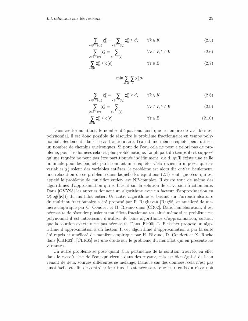
Dans ces formulations, le nombre d’équations ainsi que le nombre de variables estpolynomial, il est donc possible de résoudre le problème fractionnaire en temps poly-nomial. Seulement, dans le cas fractionnaire, l’eau d’une même requête peut utiliserun nombre de chemins quelconques. Si pour de l’eau cela ne pose a priori pas de pro-blème, pour les données cela est plus problématique. La plupart du temps il est supposéqu’une requête ne peut pas être partitionnée indéfiniment, c.à.d. qu’il existe une tailleminimale pour les paquets partitionnant une requête. Cela revient à imposer que lesvariables χe
k soient des variables entières, le problème est alors dit entier. Seulement,une relaxation de ce problème dans laquelle les équations (2.1) sont ignorées -qui estappelé le problème de multiflot entier- est NP-complet. Il existe tout de même desalgorithmes d’approximation qui se basent sur la solution de sa version fractionnaire.Dans [GVY93] les auteurs donnent un algorithme avec un facteur d’approximation enO(log(|K|)) du multiflot entier. Un autre algorithme se basant sur l’arrondi aléatoiredu multiflot fractionnaire a été proposé par P. Raghavan [Rag88] et amélioré de ma-nière empirique par C. Coudert et H. Rivano dans [CR02]. Dans l’amélioration, il estnécessaire de résoudre plusieurs multiflots fractionnaires, ainsi même si ce problème estpolynomial il est intéressant d’utiliser de bons algorithmes d’approximation, surtoutque la solution exacte n’est pas nécessaire. Dans [Fle00], L. Fleischer propose un algo-rithme d’approximation à un facteur ε, cet algorithme d’approximation a par la suiteété repris et amélioré de manière empirique par H. Rivano, D. Coudert et X. Rochedans [CRR03]. [CLR05] est une étude sur le problème du multiflot qui en présente lesvariantes.
Un autre problème se pose quant à la pertinence de la solution trouvée, en effetdans le cas où c’est de l’eau qui circule dans des tuyaux, cela est bien égal si de l’eauvenant de deux sources différentes se mélange. Dans le cas des données, cela n’est pasaussi facile et afin de contrôler leur flux, il est nécessaire que les nœuds du réseau où

26 Notions de base
cela a lieu soient équipés de manière adéquate. Ainsi avant d’écrire nos modèles, leshypothèses faites sur les équipements présents à chacun des nœuds seront présentées.

Chapitre 3
Conception de réseaux tolérantsaux pannes
Dans ce chapitre, je présente un problème de conception de réseau. L’objectifest de concevoir des réseaux aussi petits que possible capables de router des signauxprovenant de ports d’entrées vers des ports de sorties. Seulement, les entrées etsorties utilisées varient. Le rôle du réseau est, pour un nombre de signaux donnés,d’assurer l’existence d’un routage quelles que soient les entrées et sorties utilisées. Jecommence par donner la motivation du problème et faire un rappel des principauxrésultats connus avant de présenter des constructions pour différentes variantes duproblème ainsi que des bornes inférieures sur la taille des réseaux.
Le problème que je présente dans cette section a été posé par Alcatel Space Indus-trie dans les années 1995 pour des satellites destinés à des transmissions télévisuellescomme les satellites des séries Eutelsat et Astra, et reste d’actualité. Le rôle de cessatellites est de recevoir un signal vidéo et de le réémettre en direction de la terre. Leproblème concerne des réseaux destinés à ces satellites. Le but de ces réseaux est deconnecter certaines de ses entrées (sur lesquelles le satellite reçoit des signaux) à desamplificateurs (pour réémettre les signaux reçus). Les connexions se font à l’aide de latechnologie "Traveling Wave Tube Amplifiers" TWTA [EH78]. Par commodité, j’appelleles amplificateurs des sorties dans le reste de la section. À l’intérieur du satellite, lessignaux sont sous la forme d’ondes, ainsi les ports d’entrées sont reliés aux sorties autravers d’un réseau de guides d’onde. De plus les amplificateurs ne sont pas équipés decomposants permettant de séparer deux ondes différentes. Ainsi, les connexions entreles entrées et les sorties doivent s’établir via des chemins disjoints en terme de guidesd’onde. Enfin, pour des raisons d’ingénierie, les guides d’onde sont interconnectés pardes commutateurs à quatre entrées, chacun pesant 100g, ce qui est non négligeable
27

28 Réseaux tolérants aux pannes
dans le poids total du satellite à envoyer dans l’espace. Les connexions qu’un commu-tateur peut réaliser sont représentées sur la Figure 3.1.
1
3
1
3
4 2 4 2
3
1 1
24
3
24
Fig. 3.1 – Un commutateur possède quatre états différents.
Au cours de la durée de vie d’un satellite, des commutateurs peuvent se bloquerdans une position donnée, limitant ainsi les connexions réalisables. De plus, des entréespeuvent être inutilisables si le satellite est mal orienté et des sorties peuvent tomber enpanne. Dans tous les cas il est impossible de les réparer. Il est donc indispensable demettre plus de ports d’entrées et de sorties que de signaux à router. Deux variantes de ceproblème existent, dans la première variante, introduite par E. Darrot [Dar97] au coursde sa thèse, tous les signaux à router ont la même priorité ; dans la deuxième variante,certains signaux sont plus importants que d’autres. De tels signaux sont appelés dessignaux prioritaires et ils doivent être routés vers les amplificateurs assurant le meilleurservice. Les travaux que je présente ont été réalisés dans le cas où tous les signauxsont équivalents mais il est important de noter que des travaux ont été effectués surla deuxième problématique. Ainsi, dans [Hav06, BHT06], les auteurs proposent, pourun nombre de pannes maximum en sortie donné et un nombre de signaux prioritairesdonné, des réseaux de faible taille en terme de nombre de commutateurs. Ils proposentaussi pour certains cas pratiques (jusqu’à quatre signaux prioritaires et deux pannes ensorties) des réseaux de taille minimale. En effet, il est crucial de concevoir des réseauxayant aussi peu de commutateurs que possible afin de réduire le coût des satellites.Le coût total induit par un commutateur (construction et lancement) était estiméà 15 000 ¤.
Il existe d’autre contraintes qui peuvent être prises en compte comme la distanceparcourue par un signal, que ce soit en terme de nombre de commutateurs traversésou en terme de longueur physique. Dans ce dernier cas, la représentation du réseaudevient une contrainte. Le nombre de commutateurs à actionner lorsqu’une entrée ouune sortie tombe en panne influence l’énergie utilisée par le satellite, il peut donc aussiêtre intéressant de le rajouter comme contrainte. Cependant le travail que je présentes’inscrit dans la continuité des travaux déjà réalisés dans la thèse de E. Darrot [Dar97]et dans [BDD02], ainsi l’objectif est de minimiser le nombre de commutateurs.
C’est de cette contrainte sur la taille du réseau que provient la difficulté du problème.En effet, si la taille n’avait pas été une contrainte il aurait été possible de construiredes réseaux à l’aide de graphes qui ont déjà largement été étudiés : les concentrateurset les superconcentrateurs. Avant d’expliquer comment ils peuvent être utilisés pournotre problème, je vais donner leur définition ainsi que celle des graphes d’expansion,un autre type de graphes qui sera utile. Ensuite, je formaliserai le problème que jeprésente.
Concentrateurs, superconcentrateurs et graphes d’expansion 29
3.1 Concentrateurs, superconcentrateurs et graphes d’ex-pansion
Une introduction sur les concentrateurs, les superconcentrateurs et les graphesd’expansion peut être trouvée dans [DN01]. Les définitions et les différents résultatsconnus y sont donnés ainsi que des questions ouvertes. Je rappelle ci-dessous les défi-nitions ainsi que les principaux résultats dont j’ai besoin.
Les concentrateurs ont été introduits par M. Pinsker dans [Pin73] dans le cadredes réseaux de téléphone. Un (p+k, p)-concentrateur est un graphe orienté acycliqueayant p+ k entrées et p sorties, tel que pour tout ensemble de p entrées il existe pchemins arcs disjoints reliant les p entrées sélectionnées aux p sorties.
Un (p, p)-superconcentrateur, dont la définition a été introduite par A.V. Aho,J.E. Hopcroft et J.D. Ullman dans [AHU74], est aussi un graphe orienté acyclique.Les superconcentrateurs ont été introduits dans l’espoir d’établir des bornes non li-néaires sur la complexité des circuits calculant des fonctions booléennes. Un (p, p)-superconcentrateur a p entrées et p sorties ; pour tout ensemble de i ≤ p entrées eti sorties, il existe i chemins arcs disjoints reliant les entrées sélectionnées aux sortiessélectionnées.
Pour les concentrateurs comme pour les superconcentrateurs, l’objectif est d’enconstruire avec le moins d’arcs possible.
Dans [Val75] L.G. Valiant montre pour la première fois qu’il existe des supercon-centrateurs de taille linéaire (il montre qu’il en existe ayant de l’ordre de 238n arêtes),contredisant ainsi plusieurs conjectures de [AHU74]. Le lecteur intéressé pourra aussise rapporter au travail de N. Pippenger [Pip77] dans lequel l’auteur montre l’existencede (n,n)-superconcentrateurs ayant 39n+O(logn) arêtes, profondeur O(logn), et degrémaximum (entrant et sortant) 16. Ce résultat a par la suite été amélioré plusieurs fois.Ainsi, U. Schöning montre l’existence de superconcentrateurs ayant de l’ordre de 28narêtes dans [Sch06], ce résultat est pour le moment le meilleur connu. Cependant cesarticles ne donnent pas de preuve constructive, pour une construction explicite d’unsuperconcentrateur, il faudra se référer à [AC03] dans lequel les auteurs présentent lesplus petits superconcentrateurs explicites connus qui ont 44n+ o(1) arêtes. D’autresconstructions peuvent être trouvées dans [AM84, AGM87]. D’autre part, la meilleureborne inférieure connue sur le nombre d’arêtes d’un superconcentrateur est due à G.Lev et L.G. Valiant dans [LV83] et est de (5−o(1))n.
Les graphes d’expansion sont aussi très fortement liés aux réseaux étudiés dans cettesection. Le lien entre les graphes d’expansion et nos réseaux est dû à la Proposition3.1. En effet celle-ci exprime que le nombre d’arcs partant d’un sous-ensemble W doitêtre assez grand pour évacuer les signaux qui ne sont pas routés d’une entrée de Wvers une sortie de W. Un (n,d,C)-graphe d’expansion est un graphe d régulier à nsommets tel que tout ensemble de sommets S de taille au plus n/2, a au moins C · |S|arêtes sortantes. Des exemples de graphes d’expansion bien connus sont les graphesde Ramanujan, c.f. [Mor94, DSV03], qui sont des (n,d,C)-graphes d’expansion ayantun coefficient d’expansion C = 1/2(d− 2
√d−1), ce qui est le plus grand coefficient
d’expansion qu’un graphe d-régulier puisse avoir. Il existe des constructions explicites

30 Réseaux tolérants aux pannes
de graphes d’expansion pour d = q+ 1 où q est la puissance d’un nombre premier etdonc en particulier pour d = 3 et d = 4 qui sont les cas qui, dans [AGHP], nous ont servipour construire des réseaux. Dans le cas général, trouver le coefficient d’expansion d’ungraphe est NP-dur mais il est intéressant de noter que N. Alon démontre une conditionnécessaire et suffisante pour qu’un graphe régulier biparti soit un graphe d’expansiondans [Alo86].
3.2 Réseaux (p,λ,k)
Notre problème peut être formalisé de la façon suivante : étant donnés p, λ et k où preprésente le nombre de signaux reçus par le satellite, λ le nombre d’entrées inutilisableset k le nombre de sorties superflues (c.à.d. le nombre de pannes en entrées et en sortiestolérées), un réseau (p,λ,k) est un triplet (V,E), i,o où (V,E) est un graphe, i et osont des fonctions entières positives définies sur V appelées fonctions d’entrées et desorties et qui vérifient les propriétés suivantes :
– les sommets du graphe représentent les commutateurs qui ont quatre sorties, doncpour tout sommet v∈V, i(v)+o(v)+deg(v) ≤ 4.
– le nombre d’entrées est i(V) = ∑v∈V i(v) = p+ λ– le nombre de sorties est o(V) = ∑v∈V o(v) = p+k
De plus, le graphe doit vérifier la propriété que quelles que soient p des p+λ entrées etp des p+k sorties fonctionnelles, il existe p chemins arêtes disjoints reliant les p entréesaux p sorties. Cette dernière propriété est équivalente à la propriété suivante appelléepropriété de coupe :
Proposition 3.1 Un réseau (p,λ,k) vérifie, pour tout sous-ensemble W ⊂V, l’excèsde W, défini par ε(W) := δ(W)+o(W)−min(k,o(W))−min(i(W), p), est positif : ε(W)≥0.
Cette propriété peut être comprise de la manière suivante : tout signal arrivantdans un sous-ensemble de sommets W doit, soit être routé vers une sortie fonctionnelleà l’intérieur de W (il y en a au moins o(W)−min(k,o(W))), soit évacué de W par undes δ(W) liens sortants.
Ainsi pour vérifier qu’un réseau est bien un réseau (p,λ,k), il est possible, soit derésoudre un problème de flot pour chaque configuration des pannes, soit de vérifier cetinvariant pour chaque sous-ensemble de sommets. Par sous-modularité de ε il est mêmepossible de se restreindre aux sous-ensembles de sommets qui ont un complémentaireconnexe.
N (p,λ,k) désigne le nombre minimum de commutateurs nécessaire pour construireun réseau (p,λ,k). Le problème de conception de réseaux consiste à déterminerN (p,λ,k) et à construire des réseaux (p,λ,k) minimaux.

Réseaux (p,λ,k) 31
Problème 3.2 (Conception de réseaux)Entrées : Un nombre de signaux à router p.
Un nombre d’entrées p+ λ.Un nombre de sorties p+k.
Sortie : Un réseau permettant de relier p entrées à p sorties quelles que soientles λ entrées et k sorties non fonctionnelles.
Objectif : Minimiser la taille du réseau.
Ce problème a initialement été étudié par E. Darrot au cours de sa thèse et dans[BDD02] dans le cas particulier où λ = 0. Dans ce contexte, un réseau (p,0,k) est aussiappelé un (p, p+k)-sélecteur.
Pour fixer les idées, je présente maintenant quelque exemples. Dans toutes les fi-gures, les entrées sont représentées par des flèches et les sorties par des carrés. Le réseaureprésenté dans la Figure 3.2 est un réseau (3,1,1), c.à.d. un réseau capable de routertrois signaux et ce même si une des entrées et une des sorties ne sont pas fonctionnelles.Les Figures 3.3 montrent que ce réseau est bien valide dans la mesure où, quelles quesoient l’entrée et la sortie indisponibles, il est possible de router les trois signaux entrantvers les trois sorties disponibles avec trois chemins arêtes disjoints. La Figure 3.2 repré-sente un (4,8)-sélecteur, autrement dit un réseau (4,0,4). En effet, quelles que soient lesquatre sorties en panne il est possible de router quatre signaux. La Figure 3.2 illustredeux des différentes situations possibles, le lecteur peut aisément finir de se convaincrede la validité de ce réseau en envisageant les autres situations possibles.
Fig. 3.2 – Un réseau (3,1,1).
Fig. 3.3 – Validité du réseau (3,1,1).

32 Réseaux tolérants aux pannes
(a) Un réseau (4,0,4). (b) Validité du réseau (4,0,4).
Fig. 3.4 – Un réseau (4,0,4) et sa validité.
Utilisation des concentrateurs et des superconcentrateurs. Maintenant quej’ai donné les définitions d’un concentrateur et d’un sélecteur, il est clair qu’un concen-trateur :
– dont le rôle des sorties et des entrées est échangé,– dont l’orientation des arcs est ignorée,– et qui est modifié pour tenir compte de la contrainte de degré,
donne un sélecteur. De même, il est clair qu’un superconcentrateur dont l’orientationdes arcs est ignorée est un réseau (p,λ,k) pour toute valeur de k = λ, une fois modifiépour tenir compte de la contrainte de degré. Enfin, pour étendre ces constructions àdes valeurs de λ < k, il suffit d’ignorer certaines des entrées. Cependant, si minimiserle nombre de commutateurs est proche du fait de minimiser le nombre d’arcs car seulssont considérés des commutateurs de degré quatre, les sélecteurs et les réseaux (p,k,k)obtenus à l’aide de concentrateurs et de superconcentrateurs ne sont pas minimaux.Une des différences principales entre les superconcentrateurs et les réseaux (p,λ,k) estque le nombre d’entrées et de sorties qui peuvent tomber en panne dans le cadre desréseaux (p,λ,k) est borné. Le problème de concevoir des réseaux (p,λ,k) minimauxexiste donc bel et bien.
Les réseaux (p,λ,k) et le problème posé par Alcatel. Cependant avant de conti-nuer, il est important de se convaincre qu’un réseau (p,λ,k) peut effectivement êtreutilisé pour les satellites d’Alcatel. En effet, dans la définition d’un réseau (p,λ,k) uneseule contrainte sur les chemins reliant les entrées aux sorties est imposée : qu’ils soientarêtes disjoints. Or, dans le problème initialement posé par Alcatel, il y a une autrecontrainte : deux signaux ne peuvent pas se croiser n’importe comment car un commu-tateur ne peut pas connecter ses ports opposés simultanément (c.f. Figure 3.1). Dans lecas où certain signaux sont prioritaires cela est alors une contrainte, mais lorsque tousles signaux sont équivalents, cela n’en est plus une. En effet, considérons le cas d’un
Résultats antérieurs 33
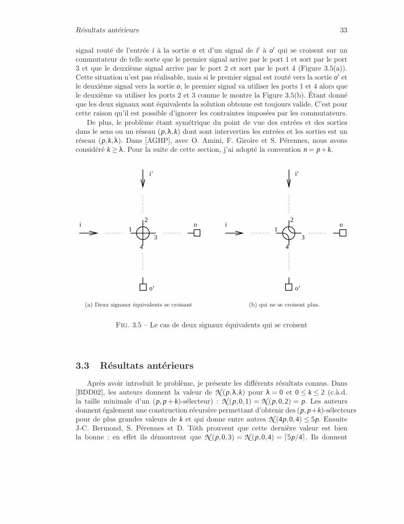
signal routé de l’entrée i à la sortie o et d’un signal de i′ à o′ qui se croisent sur uncommutateur de telle sorte que le premier signal arrive par le port 1 et sort par le port3 et que le deuxième signal arrive par le port 2 et sort par le port 4 (Figure 3.5(a)).Cette situation n’est pas réalisable, mais si le premier signal est routé vers la sortie o′ etle deuxième signal vers la sortie o, le premier signal va utiliser les ports 1 et 4 alors quele deuxième va utiliser les ports 2 et 3 comme le montre la Figure 3.5(b). Étant donnéque les deux signaux sont équivalents la solution obtenue est toujours valide. C’est pourcette raison qu’il est possible d’ignorer les contraintes imposées par les commutateurs.
De plus, le problème étant symétrique du point de vue des entrées et des sortiesdans le sens ou un réseau (p,λ,k) dont sont interverties les entrées et les sorties est unréseau (p,k,λ). Dans [AGHP], avec O. Amini, F. Giroire et S. Pérennes, nous avonsconsidéré k≥ λ. Pour la suite de cette section, j’ai adopté la convention n = p+k.
i
i’
o
o’
1
2
3
4
(a) Deux signaux équivalents se croisant
i
i’
o
o’
1
2
3
4
(b) qui ne se croisent plus.
Fig. 3.5 – Le cas de deux signaux équivalents qui se croisent
3.3 Résultats antérieurs
Après avoir introduit le problème, je présente les différents résultats connus. Dans[BDD02], les auteurs donnent la valeur de N (p,λ,k) pour λ = 0 et 0 ≤ k ≤ 2 (c.à.d.la taille minimale d’un (p, p+ k)-sélecteur) : N (p,0,1) = N (p,0,2) = p. Les auteursdonnent également une construction récursive permettant d’obtenir des (p, p+k)-sélecteurspour de plus grandes valeurs de k et qui donne entre autres N (4p,0,4) ≤ 5p. EnsuiteJ-C. Bermond, S. Pérennes et D. Tóth prouvent que cette dernière valeur est bienla bonne : en effet ils démontrent que N (p,0,3) = N (p,0,4) = ⌈5p/4⌉. Ils donnent

34 Réseaux tolérants aux pannes
également les résultats asymptotiques suivants : N (p,0,6) = ⌈5p/4⌉+√
p/8+ O(1),N (p,0,8) = ⌈4p/3⌉+2/3
√
p/3+O(p1/4) et N (p,0,10) = 11p/8+Θ(√
p). Pour les plusgrandes valeurs de k ils montrent que N (p,0,k) = 3p/2+ k/2 et que cette borne estasymptotiquement serrée. D’autres résultats sur les sélecteurs peuvent être trouvésdans [Hav06]. F. Havet y étudie le cas où le nombre de pannes tolérées est élevé parrapport au nombre d’entrées. Il montre que pour un réseau destiné à router p signaux ettolérant k pannes en sorties (0 en entrées), si p≥ k, N (p,0,k)≤ n/2+17p+O(log(n)) etsi p≤ k, N (p,0,k) ≤ 17n−16p+O(log(n)). Je rappelle la convention n= p+k. F. Havetmontre également deux bornes inférieures suivant si le nombre d’entrées est pair ouimpair :
– si le nombre d’entrées p est pair : N (p,0,k) ≥ (2p/2−1)/2p/2n+ Θ(1),– si p est impair : N (p,0,k) ≥ (2(p+1)/2−3)/2(p+1)/2n+ Θ(1).Il conjecture que cette dernière borne inférieure est en fait la bonne valeur et le
prouve dans le cas où le nombre d’entrées est petit (de 1 à 6). Si le problème généraldans lequel les λ > 0 est cité dans [BDD02], les premiers résultats sont obtenus par J-C.Bermond, F. Giroire et S. Pérennes dans [BGP07]. Ils donnent la valeur de N (p,λ,k)pour de petites valeurs de k et λ :
– N (p,1,2) =N (p,2,2) = p+2.– pour k = 3 ou k = 4, 0 < λ ≤ k, N (p,λ,k) = ⌈5n/4⌉.– pour k = 5 ou k = 6, 0 < λ ≤ k, N (p,λ,k) ≤ ⌈3n/2⌉.
3.4 Réseaux tolérant un grand nombre de pannes : contri-butions
Dans l’article [AGHP] présent dans l’Annexe A.1, avec O. Amini, F. Giroire et S.Pérennes, nous avons étudié le problème de conception de réseaux dans le cas où lenombre de pannes peut être élevé. De plus, nous avons introduit une variante, diteproblème de conception de réseaux simplifiés qui est étudiée dans les mêmesconditions. Un réseau (p,λ,k) simplifié est tel que p+ λ commutateurs sont reliés àexactement une entrée et une sortie (de tels commutateurs sont appelés des doublons,c.f. Figure 3.6) et k−λ commutateurs ont une sortie.
Fig. 3.6 – Un commutateur ayant une entrée et une sortie : un doublon.
Comme le signale déjà les auteurs de [BDD02] dans la conclusion, les réseaux ditssimplifiés sont intéressants pour les applications pour plusieurs raisons. En effet, ils ontun processus de routage simple : la plupart des signaux peuvent être envoyés sur la sortie
Réseaux tolérant un grand nombre de pannes : contributions 35
présente sur le même commutateur. De plus, dans ce routage, les chemins empruntés parles signaux sont très courts et donc minimisent l’atténuation des signaux. Ces cheminslimitent également les interférences entre signaux.
Concernant les preuves des résultats obtenus, le lecteur intéressé peut lire l’article[AGHP] présent en Annexe A.1, je me contente de présenter ici ces résultats, c.à.d.plusieurs bornes inférieures et supérieures sur la taille minimale des réseaux (p,λ,k) etdes réseaux (p,λ,k) simplifiés. Dans de nombreux cas, ces bornes donnent asymptoti-quement la taille minimale des réseaux (p,λ,k) et des réseaux (p,λ,k) simplifiés.
Afin d’obtenir les bornes inférieures, dans [AGHP] nous avons utilisé une nouvelletechnique : la quasi-partition qui dépend du Lemme 3.4. Pour pouvoir exposer ce lemme,j’ai besoin de la définition suivante :
Définition 3.3 (q-quasi-partition) Soit G = (V,E) un graphe et q un entier positif.une q-quasi-partition de G est une famille Q= A1,A2, . . . ,Am de sous-ensembles de V,telle que :
(i) pour tout 1≤ i ≤ m, le sous graphe G[Ai] induit par Ai est connexe ;(ii) pour tout 1≤ i ≤ m, q
3 ≤ |Ai| ≤ q ;(iii) V =
Smi=1 Ai et ∑m
i=1 |Ai| ≤ |V|+ |Ai; |Ai| > 2q3 |+1.
Lemme 3.4 ([DHMP06]) Soit q un entier positif et G un graphe connexe de tailleau moins q
3. G admet une q-quasi-partition.
Bornes inférieures. Le Lemme 3.4 permet d’obtenir des informations sur l’ensembledu réseaux à partir d’observations locales. Il sert pour prouver le théorème suivant :
Théorème 3.5 Dans un réseau (p,λ,k) de taille N, pour k≤ n2 :
N ≥(
32n− (k−λ)−4− 12√
k
)(
1− 92√
k+O
(
1k
)
)
+ d2
(
1+ 92√
k+O
(
1k
)
)
.
avec n = p+k et d le nombre de doublons, c.à.d. le nombre de commutateurs ayantexactement une entrée et une sortie.
Ce théorème est ensuite utilisé pour obtenir des bornes inférieures pour les différentsproblèmes. Dans le cas général, il donne le Corollaire 3.6 :
Corollaire 3.6 (Cas Général). Pour λ → ∞ et k → ∞, un réseau (p,λ,k) contient aumoins n+ 2
3n+O( n√λ) commutateurs. Autrement dit, N (p,λ,k) ≥ n+ 2
3n+O( n√λ).

36 Réseaux tolérants aux pannes
Dans le cas où le réseau ne tolère pas les pannes d’entrées, c.à.d. quand λ = 0, ouencore le cas des sélecteurs, cela donne le Corollaire 3.7.
Corollaire 3.7 (Sélecteurs, λ = 0). Dans un réseau (p,0,k) de taille N, pour k→ ∞ etk≤ n
2, on a :
N ≥ n+n2
+O(n√k)
Autrement dit :N (p,0,k) ≥ n+
n2
+O(n√k).
Enfin dans le cas dit simplifié, cela donne le Corollaire 3.8.
Corollaire 3.8 (Cas simplifié). Dans un réseau (p,λ,k) simplifié, pour k→ ∞ et k≤ n2,
il y a au moins 2n+ O( n√k) commutateurs, c.à.d. N (p,λ,k) ≥ 2n+ O( n√
k) dans le cas
simplifié.
Bornes supérieures. Pour montrer des bornes supérieures, dans [AGHP], nousconstruisons des réseaux (p,λ,k) à l’aide de graphes d’expansion. Seulement les ré-seaux construits de cette façon ne sont valables que pour des valeurs de k et λ bornéespar logn. L’ensemble des bornes supérieures est listé ci-dessous :
Théorème 3.9 (Cas général). Pour n= p+k, k≤ 115 logn, et n assez grand : N(p,λ,k)≤
n+ 34n
Nous faisons d’ailleurs la conjecture que cette borne supérieure est la valeur deN (p,λ,k).
Conjecture 3.10 Pour n = p+k, k≤ 115 logn, et n assez grand : N(p,λ,k) = n+ 3
4n
Théorème 3.11 (Sélecteurs, λ = 0). Pour n = p+k, k≤ 148 log2 n, et n assez grand :
N(p,0,k) ≤ n+n2.
Théorème 3.12 (Cas simplifié). Pour n= p+k, k≤ 16 logn, et n assez grand : N(p,λ,k)≤
2n.
Les résultats antérieurs ne donnaient la valeur de N (p,λ,k) que dans le cas desréseaux tolérant un nombre de pannes maximum borné par une constante, ainsi cesderniers théorèmes apportent des informations nouvelles en donnant la valeur asymp-totique de N (p,λ,k) pour des valeurs plus grandes de k. Cependant k reste borné parlogn. Afin d’obtenir des résultats pour des valeurs de k plus grande encore, nous avonsdéfini un nouveau paramètre appelé l’α-robustesse. Le but de ce paramètre est d’éva-luer l’expansion locale d’un graphe. Étant donné un réel α, l’α−robustesse d’un graphe,

Réseaux tolérant un grand nombre de pannes : contributions 37
rα, est le plus grand entier tel que pour tout sous-ensemble X ⊂V de taille |X| ≤ |V|/2,on a :
δ(X) ≥ min(α|X|, rα).
Cela signifie que les petits ensembles ont un facteur d’expansion α alors que les plusgrands ensembles (de taille plus grande que rα/α) ont au moins rα arêtes sortantes.Cette notion diffère des approches usuelles dans la mesure où, au lieu de chercher lecoefficient d’expansion d’un graphe, un coefficient d’expansion est fixé et le but est dechercher quels sont les ensembles qui le vérifient. Des notions proches sont présentéesdans [CRVW02, AHK99].
Liens entre la robustesse et d’autres paramètres. Cette définition est motivéepar le fait qu’un réseau (p,λ,k) n’a pas besoin de vérifier de bonnes propriétés d’expan-sion pour les grands ensembles de sommets. Cette notion est également intéressante enelle-même et généralise plusieurs invariants comme la bisection-width et la constante deCheeger ([Chu97]). Je rappelle que la bisection-width est le plus petit nombre d’arêtesentre les deux ensembles d’une partition des sommets en deux ensembles de même taille.Elle a entre autres été étudiée par N. Alon dans [Alo93] et par B. Moniens et R. Preisdans [MP06]. L’α-robustesse est également reliée à la notion de graphe d’expansion, parexemple les graphes de Ramanujan qui ont un facteur d’expansion 1/2(d−2
√d−1) ont
une 1/2(d−2√
d−1)-robustesse de n/2.
Application de l’α-robustesse. Pour construire des réseaux (p,λ,k), il faut desgraphes ayant une bonne 1-robustesse. Comme la robustesse est une notion proche del’expansion et qu’il se trouve que les graphes aléatoires sont de bons graphes d’expan-sion, dans [AGHP], nous avons étudié l’α−robustesse des graphes aléatoires 4-réguliers.Nous y généralisons des résultats de B. Bollobàs sur leurs coefficients d’expansion([Bol88]). Nous n’avons pas trouvé d’articles antérieurs parlant de ce concept d’ex-pansion locale, et les résultats que nous obtenons nous permettent de construire desréseaux (p,λ,k) ayant 3n commutateurs et tolérant jusqu’à n/7 pannes (d’entrées commede sorties). Je présente ces preuves dans la Section 3.4.1. Elles peuvent également êtretrouvées dans la thèse de F. Giroire [Gir06] ou dans l’Annexe A.1.
Théorème 3.13 Les graphes aléatoires 4-réguliers ont une 1-robustesse d’au moinsn/14 avec probabilité 1−O( logn
n ).
Corollaire 3.14 Pour k≤ n7, il existe un réseau (p,λ,k) de taille 3n où n = p+k.
Preuve. Soit G un graphe Hamiltonien 4-régulier sur 2n sommets ayant une 1-robustessed’au moins n/7. Si un doublon (en bleu sur la Figure 3.7) est rajouté à chaque arêted’un couplage parfait (en pointillés rouges) obtenu à partir d’un cycle Hamiltonien, celadonne un réseau (p = n−k,k,k) pour tout k≤ n/7 qui a 3n sommets.
Il est facile de vérifier que c’est bien un réseau (p,λ,k) à l’aide de la Propriété 3.1.Cette construction peut se généraliser pour tout k ≤ n/2 si les arêtes auxquelles lesdoublons sont rajoutés, sont choisies à bonne distance. 2
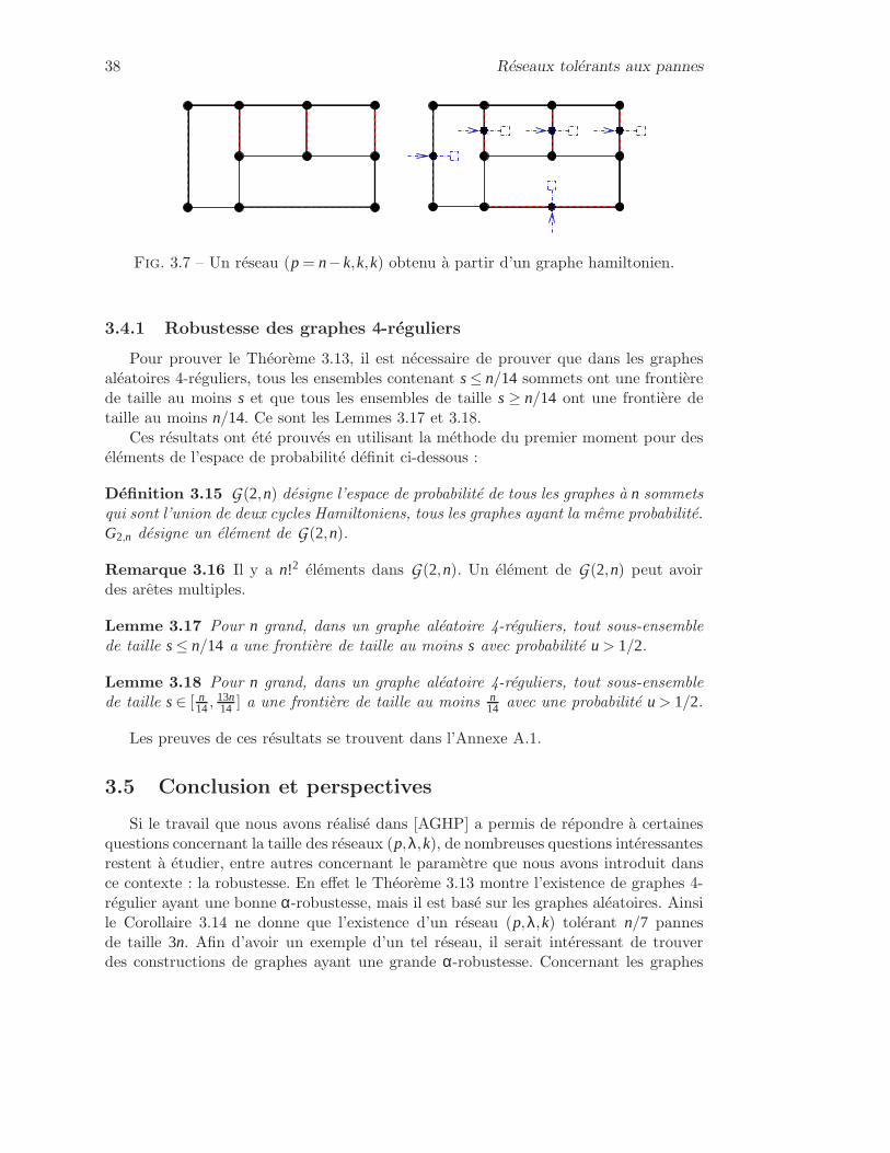
38 Réseaux tolérants aux pannes
Fig. 3.7 – Un réseau (p = n−k,k,k) obtenu à partir d’un graphe hamiltonien.
3.4.1 Robustesse des graphes 4-réguliers
Pour prouver le Théorème 3.13, il est nécessaire de prouver que dans les graphesaléatoires 4-réguliers, tous les ensembles contenant s≤ n/14 sommets ont une frontièrede taille au moins s et que tous les ensembles de taille s≥ n/14 ont une frontière detaille au moins n/14. Ce sont les Lemmes 3.17 et 3.18.
Ces résultats ont été prouvés en utilisant la méthode du premier moment pour deséléments de l’espace de probabilité définit ci-dessous :
Définition 3.15 G(2,n) désigne l’espace de probabilité de tous les graphes à n sommetsqui sont l’union de deux cycles Hamiltoniens, tous les graphes ayant la même probabilité.G2,n désigne un élément de G(2,n).
Remarque 3.16 Il y a n!2 éléments dans G(2,n). Un élément de G(2,n) peut avoirdes arêtes multiples.
Lemme 3.17 Pour n grand, dans un graphe aléatoire 4-réguliers, tout sous-ensemblede taille s≤ n/14 a une frontière de taille au moins s avec probabilité u > 1/2.
Lemme 3.18 Pour n grand, dans un graphe aléatoire 4-réguliers, tout sous-ensemblede taille s∈ [ n
14,13n14 ] a une frontière de taille au moins n
14 avec une probabilité u > 1/2.
Les preuves de ces résultats se trouvent dans l’Annexe A.1.
3.5 Conclusion et perspectives
Si le travail que nous avons réalisé dans [AGHP] a permis de répondre à certainesquestions concernant la taille des réseaux (p,λ,k), de nombreuses questions intéressantesrestent à étudier, entre autres concernant le paramètre que nous avons introduit dansce contexte : la robustesse. En effet le Théorème 3.13 montre l’existence de graphes 4-régulier ayant une bonne α-robustesse, mais il est basé sur les graphes aléatoires. Ainsile Corollaire 3.14 ne donne que l’existence d’un réseau (p,λ,k) tolérant n/7 pannesde taille 3n. Afin d’avoir un exemple d’un tel réseau, il serait intéressant de trouverdes constructions de graphes ayant une grande α-robustesse. Concernant les graphes
Conclusion et perspectives 39
d’expansion, il est possible d’en construire à l’aide du produit Zigzag qui a été introduitpar [RVW02] ou par le "lift" de [BL06], il est donc naturel de se demander si destechniques similaires permettent d’obtenir des graphes ayant une bonne robustesse.
Précédemment nous avons dit que l’α-robustesse généralise la bisection-width. Dans[MP06], les auteurs montrent que la bisection-width maximale d’un graphe à n sommetsest au plus 2n/5. Cela implique que l’α-robustesse est au plus n
2 quand α > 45. Est-il
possible de généraliser ce résultat et, par exemple, de donner une condition sur αassurant une α-robustesse d’au plus n/3?
40 Réseaux tolérants aux pannes

Chapitre 4
Algorithmes de routage
Dans ce chapitre, je m’intéresse à la couche réseau du système OSI, c.à.d. àla couche numéro trois. Je rappelle que le but de cette couche est de gérer lesconnexions entre les différents systèmes composant le réseau. Dans la première sec-tion, je présente des algorithmes de routage optimaux pour le routage de paquetsdans les grilles hexagonales et triangulaires, pour le modèle ∆-port, half- ou full-duplex, dans le cas de la permutation, du routage r-central et du (ℓ,ℓ)-routage. Jeprésente également un algorithme d’approximation dans le cas du (ℓ,k)-routage.Dans la deuxième section, je présente des algorithmes d’approximation pour la co-loration k-impropre des graphes hexagonaux. Ce problème modélise un problèmed’affectation de fréquences pour des transmissions entre un satellite et des an-tennes. Dans la dernière section, je montre qu’un problème d’ordonnancement deconnexions dans un réseau radio sans fils maillé peut être modélisé par un problèmede coloration appelé coloration proportionnelle qui est NP-dur dans le cas général.
Étant donné un réseau et des requêtes entre les systèmes du réseau (chaque requêtecorrespond à des données à transmettre entre des systèmes), le problème consiste àorganiser le transfert de ces requêtes à l’aide des infrastructures disponibles. Ainsi,le problème dépend fortement du réseau considéré. Dans ce chapitre, le problème estétudié dans trois types de réseaux différents :
– Les premiers réseaux considérés sont des réseaux en forme de grilles qui repré-sentent typiquement des processeurs reliés entre eux.
– Les seconds réseaux considérés sont des réseaux WiFi constitués d’antennes re-cevant des signaux d’un satellite.
– Les derniers réseaux étudiés sont également des réseaux WiFi, qui sont composésde routeurs communiquant entre eux.
Dans les trois cas, je considère uniquement des requêtes émises par un système età destination de ceux-ci. Je ne porterai pas, dans ce chapitre, mon attention sur les
41
42 Algorithmes de routage
requêtes multicasts, qui seront traitées plus tard.Dans chacune des sections sont utilisées des techniques différentes. Cela illustre
la variété des approches disponibles pour résoudre des problèmes similaires. Dans lapremière section, je présente des résultats obtenus à partir d’algorithmes de type bigfoot, tandis que les problèmes des deux sections suivantes sont modélisés par deuxproblèmes différents de coloration de graphes.
4.1 Algorithmes de routage dans les grilles
Le travail que je présente dans cette section a été réalisé en collaboration avecO. Amini, I. Sau Valls et J. Žerovnik. L’article que nous avons soumis à JOIN peutêtre trouvé dans l’Annexe B.1. Le problème auquel nous nous sommes intéressés estun problème d’ordonnancement. Étant donné un ensemble de paquets, caractérisés parleur origine et leur destination, l’objectif est de trouver un chemin et un ordonnacementdes déplacements de chacun des paquets afin de tous les acheminer à leur destinationtout en minimisant le temps pris par l’acheminement de tous les paquets. Ce problèmepeut être formulé de la manière suivante :
Problème 4.1 (Problème de routage de paquets dans les réseaux)Entrées : Un réseau.
Un ensemble de paquets, chacun caractérisé par une source et unedestination.
Sorties : Un chemin pour chacun des paquets.Un ordonnancement des déplacements de chacun des paquets.
Objectif : Minimiser le temps nécessaire pour acheminer tous les paquets.
4.1.1 Contexte
En 1988, T. Leighton, B. Maggs et S. Rao prouvent dans [LMR88, LMR94], que quelque soit le réseau, pour tout ensemble de paquets dont on connait a priori les cheminssur lesquels ils vont être routés, il existe un ordonnancement permettant d’acheminertous les paquets le long de leur chemin en un temps optimal de O(C+D) étapes, où Creprésente la charge du réseau (le nombre maximum de chemins utilisant une mêmearête) et D la dilatation (la longueur du chemin le plus long).
Théorème 4.2 ([LMR88]) Pour tout ensemble de paires paquet-chemin, il existe unprotocole de routage hors-ligne nécessitant O(C+D) étapes pour router tous les paquets.
De plus, dans [ST97], les auteurs montrent qu’étant donné un ensemble de paquets,il est possible de trouver en temps polynomial un chemin pour chacun des paquets telque la valeur de C+D dans ce routage soit au plus à un facteur quatre de l’optimum.Ainsi on peut reformuler le Théorème 4.2 de manière plus générale.
Théorème 4.3 ([ST97]) Pour tout ensemble de paquets, il existe un protocole de rou-tage hors-ligne nécessitant O(C+ D) étapes pour router tous les paquets, où C+ D estle minimum de "la charge du réseau plus la dilatation" sur tous les routages.

Algorithmes de routage dans les grilles 43
Fig. 4.1 – Grilles triangulaire () et hexagonale. (9)
Qui plus est, dans l’ordonnancement obtenu, à chaque étape, le nombre de paquetsdevant être stockés par un nœud est borné par une constante.
Bien que ces résultats soient asymptotiquement les meilleurs possibles, si l’on consi-dère certains types de paquets et certains types de réseaux bien précis, il est possible deconcevoir des algorithmes qui sont plus efficaces en pratique. En effet, un gros facteurmultiplicatif peut se cacher derrière le O dans le théorème précédent.
4.1.2 Les différents scénarios de requêtes
Les différents types de scénarios pour les paquets sont définis à partir du nombre depaquets émis et reçus par chaque système du réseau. Les problèmes les plus courammentétudiés sont les suivants :
1. Permutation : chaque nœud est source et destination d’exactement un paquet.2. (ℓ,k)-routage : chaque système est source d’au plus ℓ paquets et en est destina-
tion d’au plus k. Un autre cas particulier important est le cas (1,k)-routage.3. (1, tous)-routage : chaque nœud est source d’au plus un paquet mais il n’y a pas
de contrainte sur le nombre maximum de paquets dont un nœud est destination.4. routage r-central : tous les nœuds à distance au plus r du nœud central lui
adressent un paquet.Dans chacun de ces scénarios, étant donnée une configuration initiale, l’objectif est detrouver des chemins et un ordonnancement permettant d’acheminer les paquets le plusrapidement possible.
4.1.3 Les différents types de réseaux
Topologie. Le réseau le plus étudié est la grille carrée. Une des raisons est qu’elleest utilisée dans les réseaux de processeurs. Les réseaux radios sont, quant à eux, sou-vent modélisés par des grilles hexagonales ou triangulaires dans lesquelles les nœudsreprésentent les stations de base. Avec O. Amini, I. Sau Vals et J. Žerovnik, ce sont àces trois types de grilles (carrées, triangulaires et hexagonales) que nous nous sommesintéressés dans [AHSZ08].

44 Algorithmes de routage
t
s
Fig. 4.2 – Trois directions dans la grille hexagonale et le principe de l’algorithme bigfoot.
La Figure 4.1 représente les grilles triangulaires et hexagonales. La grille hexagonaleest un sous-graphe de la grille triangulaire. La grille triangulaire peut être obtenue àpartir d’une grille carrée en rajoutant une diagonale, c’est aussi le dual de la grille hexa-gonale. Nous considérons des sous-grilles convexes (c.à.d. contenant tous les chemins lesplus courts entre deux sommets) des trois grilles carrées, triangulaires et hexagonales.
Caractéristiques des composants. Nous nous plaçons dans le modèle où chaquesystème peut stocker et retransmettre les paquets reçus (store-and-forward model).Chaque système doit donc être capable de gérer une file d’attente de paquets (queue).Chaque système peut également recevoir et envoyer des paquets sur tous les liens quile connectent au réseau en même temps (∆-port model). Enfin, nous considèrons à lafois le cas où les liens sont bidirectionnels, et ne peuvent donc être utilisés que dans unsens à chaque étape (half-duplex networks), et le cas où chaque lien représente enfait deux liens, un dans chaque sens, ce qui permet à chaque étape de transmettre desdonnées simultanément dans les deux directions (full-duplex networks).
4.1.4 Résultats connus dans la grille carrée
Je rappelle très brièvement les résultats connus concernant les grilles carrées.Dans [HLJ97], les auteurs introduisent un algorithme appelé big foot. Étant don-
nées plusieurs directions (horizontale X et verticale Y dans la grille carrée), l’idée del’algorithme est (dans une grille à deux dimensions) de router chacun des paquets aussiloin que utile le long d’une première direction puis de finir le routage en utilisant uneseconde direction. Dans une grille carrée, ce routage est également connu sous le nom deroutage XY. Les algorithmes que nous proposons utilisent ce principe, comme illustrésur la Figure 4.2, dans le cas de la grille hexagonale.
Permutation. Dans [SCK97], les auteurs proposent un algorithme trouvant un or-donnancement optimal (utilisant 2n−2 étapes) et utilisant des files d’attente de taille auplus 81. Ils proposent également un algorithme trouvant un ordonnancement utilisant
Algorithmes de routage dans les grilles 45
2n+O(1) étapes et utilisant des files d’attente de taille au plus 12.
(1,k)-routage. Dans [SK94], les auteurs proposent un algorithme donnant un ordon-nancement quasi optimal qui utilise
√kn
2 +O(n) étapes. Ils donnent un autre algorithmecalculant un ordonnancement nécessitant un peu plus d’étapes mais qui utilise des filesd’attente de taille maximale 3.
(ℓ,ℓ)-routage. Dans [SK94], les auteurs proposent également un algorithme calcu-lant des ordonnancements utilisant O(ℓn) étapes, sachant que dans [SK94], les auteursproposent une borne inférieure en Ω(
√ℓkn) pour le (ℓ,k)-routage.
(ℓ,k)-routage. Dans [PP01], les auteurs donnent des algorithmes déterministes etaléatoires permettant de calculer un ordonnancement utilisant O(
√ℓkn) étapes, ce qui
est optimal.
4.1.5 Algorithmes de routage dans les grilles hexagonales et triangu-laires : contributions
Les algorithmes que nous proposons dans [AHSZ08] (et qui peuvent être trouvésdans l’Annexe B.1) sont tous distribués, et peuvent ainsi être utilisés indépendammentpar chaque nœud. Ils utilisent tous les chemins les plus courts, ce qui permet de mi-nimiser la dilatation qui est alors la longueur du plus long plus court chemin, et estnotée ℓmax. Cependant, un routage utilisant les chemins les plus courts ne permet pastoujours d’avoir un ordonnancement utilisant le nombre minimum d’étapes.
Permutation. Nous proposons le premier algorithme permettant de calculer des or-donnancements utilisant le moins possible d’étapes dans les grilles hexagonales full-duplex (2ℓmax− 2 étapes) et half-duplex (4ℓmax− 4 étapes) ainsi que dans les grillestriangulaires half-duplex (2ℓmax étapes).
Routage r-central. Nous proposons le premier algorithme permettant de calculerdes ordonnancements utilisant le moins possible d’étapes dans les grilles carrées, hexa-gonales et triangulaires (full et half-duplex) en respectivement
(r+12
)
,(3r+1
2
)
et(6r+1
2
)
étapes pour le cas full-duplex (le double dans half-duplex).
(ℓ,ℓ)-routage. Nous proposons le premier algorithme permettant de calculer des or-donnancements utilisant le moins possible d’étapes dans les grilles carrées, hexagonales(2ℓℓmax en full-duplex) et triangulaires (ℓℓmax en full-duplex) (full et half-duplex).
(ℓ,k)-routage. Nous proposons un algorithme permettant de calculer des ordonnan-cements utilisant un nombre d’étapes à un facteur constant garanti (mais dont la for-mule n’est pas très élégante) du nombre minimum d’étapes dans les grilles carrées,hexagonales et triangulaires (full et half-duplex).
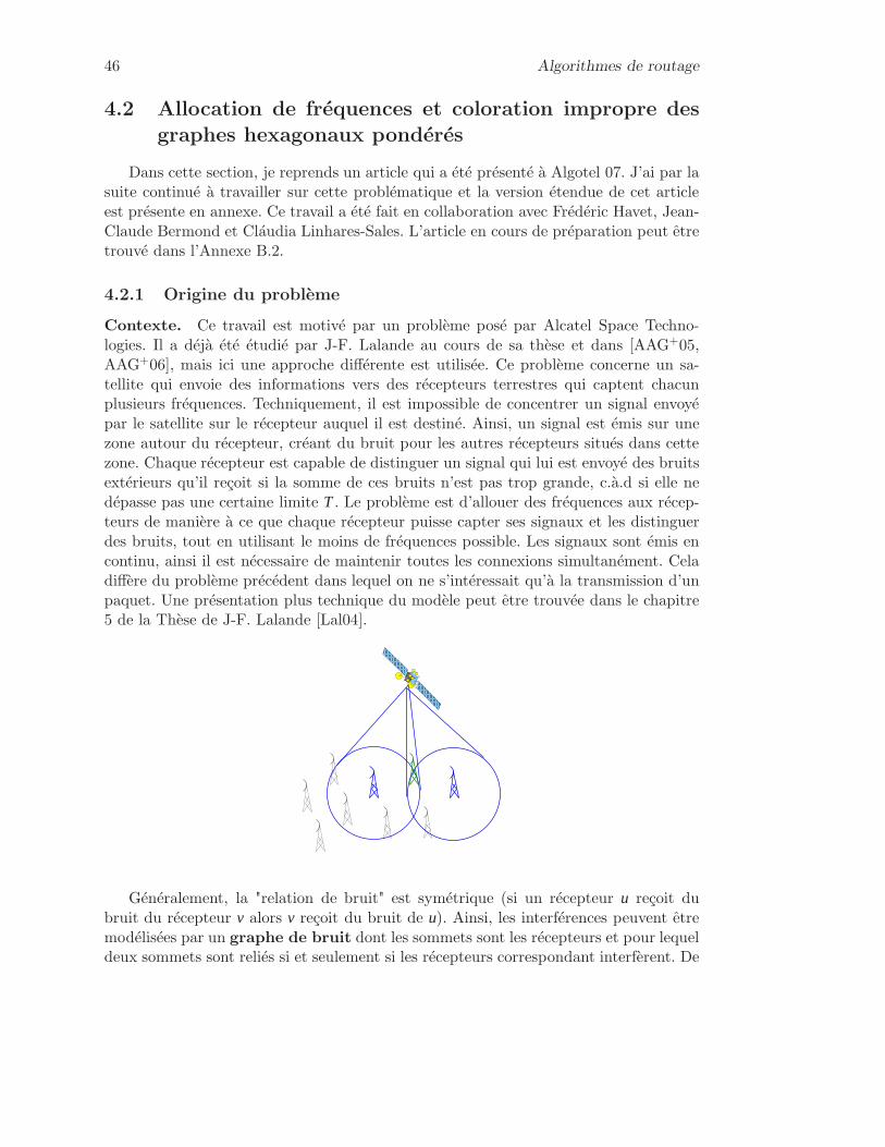
46 Algorithmes de routage
4.2 Allocation de fréquences et coloration impropre desgraphes hexagonaux pondérés
Dans cette section, je reprends un article qui a été présenté à Algotel 07. J’ai par lasuite continué à travailler sur cette problématique et la version étendue de cet articleest présente en annexe. Ce travail a été fait en collaboration avec Frédéric Havet, Jean-Claude Bermond et Cláudia Linhares-Sales. L’article en cours de préparation peut êtretrouvé dans l’Annexe B.2.
4.2.1 Origine du problème
Contexte. Ce travail est motivé par un problème posé par Alcatel Space Techno-logies. Il a déjà été étudié par J-F. Lalande au cours de sa thèse et dans [AAG+05,AAG+06], mais ici une approche différente est utilisée. Ce problème concerne un sa-tellite qui envoie des informations vers des récepteurs terrestres qui captent chacunplusieurs fréquences. Techniquement, il est impossible de concentrer un signal envoyépar le satellite sur le récepteur auquel il est destiné. Ainsi, un signal est émis sur unezone autour du récepteur, créant du bruit pour les autres récepteurs situés dans cettezone. Chaque récepteur est capable de distinguer un signal qui lui est envoyé des bruitsextérieurs qu’il reçoit si la somme de ces bruits n’est pas trop grande, c.à.d si elle nedépasse pas une certaine limite T. Le problème est d’allouer des fréquences aux récep-teurs de manière à ce que chaque récepteur puisse capter ses signaux et les distinguerdes bruits, tout en utilisant le moins de fréquences possible. Les signaux sont émis encontinu, ainsi il est nécessaire de maintenir toutes les connexions simultanément. Celadiffère du problème précédent dans lequel on ne s’intéressait qu’à la transmission d’unpaquet. Une présentation plus technique du modèle peut être trouvée dans le chapitre5 de la Thèse de J-F. Lalande [Lal04].
Généralement, la "relation de bruit" est symétrique (si un récepteur u reçoit dubruit du récepteur v alors v reçoit du bruit de u). Ainsi, les interférences peuvent êtremodélisées par un graphe de bruit dont les sommets sont les récepteurs et pour lequeldeux sommets sont reliés si et seulement si les récepteurs correspondant interfèrent. De
Allocation de fréquences et coloration impropre des graphes hexagonaux pondérés 47
plus, le graphe est muni d’une fonction de poids w : V → N, où le poids w(v) dusommet v est égal au nombre de signaux que le récepteur correspondant doit recevoir.Cela donne un graphe pondéré, c.à.d. une paire (G,w) où G est un graphe et w unefonction de poids sur les sommets de G.
Énoncé du problème. Dans une version simplifiée, l’intensité I du bruit créé estindépendante de la fréquence et du récepteur. Ainsi, pour pouvoir distinguer son signaldes bruits, un récepteur doit être dans la zone de bruit d’au plus k = ⌊T/I⌋ récepteursécoutant sur la même fréquence. Le problème revient donc à trouver une colorationdu graphe (pondéré) de bruit qui soit k-impropre. Une coloration du graphe pondéré(G,w) est une fonction C :V → P (S) telle que |C(v)| ≥w(v), l’ensemble Sétant l’ensemblede couleurs et P (S) l’ensemble des parties de S. Comme seule la cardinalité de S estintéressante, S= 1,2, . . . , l pour un certain entier l . Une coloration de (G,w) avec unensemble de couleurs de taille l est appelée l-coloration. Une coloration C de (G,w)est k-impropre si pour toute couleur i, l’ensemble des sommets ayant la couleur iinduit un graphe de degré au plus k. En d’autres termes, tout sommet recevant unecouleur i est adjacent à au plus k sommets recevant cette même couleur i. Le nombrechromatique k-impropre de (G,w), noté χk(G,w), est le plus petit entier l tel que(G,w) ait une l -coloration k-impropre. Puisque le but est de minimiser le nombre defréquences, il faut trouver une coloration k-impropre de (G,w) ayant un nombre decouleurs aussi proche que possible de l’optimum χk(G,w).
Problème 4.4 (Coloration impropre d’un graphe pondéré)Entrées : Un graphe pondéré (G,w).
Un indice d’impropreté k.Sortie : Une coloration k-impropre de (G,w).Objectif : Garantir un nombre de couleurs utilisées aussi proche que possible de
l’optimum.
Modèle utilisé. Dans le problème posé par Alcatel, la zone de réception est découpéeen cellules hexagonales, une cellule étant adjacente aux six cellules voisines. Ainsi, lesrécepteurs sont répartis comme les sommets du réseau triangulaire R, qui est représentésur la Figure 4.3, et peut être décrit comme suit : les sommets sont les combinaisonslinéaires ae1 +be2 des vecteurs e1 = (1,0) et e2 = (1
2,√
32 ) : ainsi il est possible d’identifier
les sommets avec les paires (a,b) d’entiers.Deux sommets sont adjacents si la distance euclidienne entre eux est égale à 1.
Ainsi chaque sommet x= (a,b) a six voisins : (a−1,b), (a+1,b), (a−1,b+1), (a,b+1),(a,b−1) et (a+1,b−1). Les graphes de bruit étudiés dans ce chapitre, sont des sous-graphes induits du réseau triangulaire (Figure 4.3), appelés graphes hexagonaux. LaFigure 4.4 donne une 5-coloration 1-impropre de R avec w(v) = 2 pour tout v∈V(R).
Résultats connus. Pour k≥ 6, le nombre chromatique k-impropre d’un graphe hexa-gonal est son poids maximum wmax = maxw(v) | v∈V(G) car son degré maximumest au plus 6. Ainsi seules sont étudiées des impropretés inférieures à 6. Généralisant

48 Algorithmes de routage
e
e2
1
0,0
0,1 1,1
1,0
(a+1,b)
(a−1,b+1)(a,b+1)
(a−1,b)
(a+1,b−1)(a,b−1)
Fig. 4.3 – Les récepteurs sont répartis sur les sommets d’un réseau triangulaire.
un résultat de McDiarmid et Reed [MR00] pour la coloration propre, F. Havet, Kanget J-S. Sereni [HKS05, Ser06] ont montré que pour tout 0≤ k≤ 5, il est NP-complet dedécider si le nombre chromatique k-impropre d’un graphe hexagonal pondéré est 3 ou4. Ainsi il n’existe pas d’algorithme polynomial pour trouver le nombre chromatiquek-impropre d’un graphe hexagonal pondéré (à moins que P=NP). Le but est de trouverdes algorithmes αk-approchés, c.à.d. qui trouvent une coloration k-impropre de toutgraphe hexagonal pondéré (G,w) avec au plus αk×χk(G,w)+ βk couleurs, où αk et βk
sont deux constantes.C. McDiarmid and B. Reed [MR00] ont donné un algorithme 4/3-approché pour la
coloration propre des graphes hexagonaux pondérés. Un algorithme distribué garantis-sant ce même rapport de 4/3 est donné par Narayanan et Schende [NS01].
Dans [AAG+06], les auteurs proposent une formulation mathématique, sous formede génération de colonnes, pour résoudre le problème d’affectation de longueur d’onde.
Plan. Dans cette section, je présente un algorithme αk-approché pour la colorationk-impropre des graphes hexagonaux pondérés pour tout 1≤ k≤ 5, avec α1 = 25
13, α2 = 127 ,
α3 = 1813, α4 = 80
63 et α5 = 4943. La méthode proposée pouvant être appliquée à tous les
graphes pondérés, je la présente dans un contexte général.
4.2.2 Algorithmes d’approximation
Soit q un entier. On note q la fonction de poids constante égale à q. Une méthodenaturelle pour trouver une coloration k-impropre de (G,w) consiste à trouver une colora-tion k-impropre de (G,q). Supposons que cette coloration utilise r couleurs, idéalementr = χk(G,q). les demandes sont ensuite découpées en
⌈
wmaxq
⌉
paquets de telle sorte quedans aucun des paquets un sommet ait plus de q demandes ; en utilisant r couleurs parpaquets, cela donne une coloration en r ×
⌈
wmaxq
⌉
couleurs. Comme χk(G,w)≥ wmax, cecidonne un algorithme (r/q) approché.
La prochaine étape est de déterminer le nombre chromatique k-impropre (1≤ k ≤5) du réseau triangulaire avec poids constant. C’est une borne supérieure du nombrechromatique k-impropre de tout graphe hexagonal.

Allocation de fréquences et coloration impropre des graphes hexagonaux pondérés 49
Théorème 4.5 Pour le réseau triangulaire R :(i) χ1(R,q) =
⌈
5q2
⌉
(ii) χ2(R,q) = 2q
(iii) χ3(R,q) =⌈
3q2
⌉
(iv) χ4(R,q) =⌈
4q3
⌉
(v) χ5(R,q) =⌈
7q6
⌉
1,25,14,53,41,25,1 2,3
1,25,14,53,41,25,1 2,3
1,2 4,52,33,4 3,45,14,5
1,2 4,52,33,4 3,45,14,5
1,25,14,53,41,25,1 2,3
Fig. 4.4 – Une coloration 1-impropre de (R,2)
Ces colorations donnent des algorithmes 5/2- , 2-, 3/2-, 4/3- et 7/6-approchés pourla coloration 1-, 2-, 3-, 4- et 5-impropre respectivement des graphes hexagonaux pon-dérés. Il est cependant possible de faire mieux : une coloration de (G,q) utilisant rcouleurs, donne un algorithme de coloration de (G,w) avec un rapport d’approximationmeilleur que r/q. Pour cela, au lieu de ne considérer que wmax, il faut également consi-dérer le nombre de couleurs imposé par un sommet et k+ 1 de ses voisins. Comme lemontre la proposition suivante, celui-ci peut être supérieur à wmax. Le graphe ayant unsommet u, appelé centre, adjacent à k+1 autres sommets, appelés pointes, est notéK1,k+1.
Proposition 4.6 Pour toute fonction de poids w, χk(K1,k+1,w) ≥ 1k+1 ∑
v∈V(K1,k+1)
w(v).
Preuve. Soit u le centre de K1,k+1 et v1, . . . ,vk+1 ses pointes. Considérons une colorationk-impropre C de K1,k+1. Pour tout 1≤ i ≤ k+1, soit q(vi) = |C(vi)\C(u)|. La colorationC utilise au moins M = maxq(vi)+w(u) | 1≤ i ≤ k+1 ≥ w(u)+ 1
k+1 ∑k+1i=1 q(vi). Or une
couleur de C(u) est utilisée au plus par k des vi car la coloration est k-impropre. Donc∑k+1
i=1 q(vi) ≥ ∑k+1i=1 w(vi)−kw(u). Il vient M ≥ 1
k+1(w(u)+ ∑k+1i=1 w(vi)). 2
On appelle (k+1)-étoile, ou simplement étoile, un sous-graphe de G isomorphe àK1,k+1. Le poids d’une étoile H est w(H)= ∑v∈V(H) w(v). On note θk(G,w)= maxw(H)/(k+1) | H étoile de G et ωk(G,w)= maxwmax,θk(G,w). D’après la Proposition 4.6, ωk(G,w)≤χk(G,w).
50 Algorithmes de routage
Théorème 4.7 Soient αk(r,q) = (k+1)r2
(k+2)rq−q2 et βk(r,q) = max(k+ 2)r2 − rq,(k+ 1)r2 +
krq.Étant donné une coloration C de (G,q) avec r couleurs, il existe un algorithme
polynomial qui colore (G,w) avec au plus αk(r,q)×ωk(G,w)+ βk(r,q) couleurs.
Remarques finales. Les Théorèmes 4.5 et 4.7 permettent d’obtenir un algorithmeαk-approché pour calculer la coloration k-impropre (1≤ k≤ 5) d’un graphe hexagonalpondéré. Pour k = 1 ou k = 5, il est possible d’améliorer le facteur d’approximation enanalysant plus précisément la répartition des gros sommets et des sommets contraints.Dans l’article en cours présenté en Annexe B.2, nous avons obtenu des algorithmes2011- et 41
36-approchés pour la coloration 1- et 5-impropre respectivement des grapheshexagonaux pondérés. Nous avons également des versions distribuées de chacun de cesalgorithmes. Parmi les problèmes à considérer, il est intéressant d’examiner d’autrestopologies et surtout d’autres modèles de bruit pour lesquels l’intensité dépend de ladistance et/ou de la fréquence utilisée.
4.3 Optimisation des buffers dans les réseaux radios etcoloration proportionnelle
Dans cette section, je présente un travail réalisé en collaboration avec C. LinharèsSalés et H. Rivano, sur un nouveau problème de coloration : la coloration proportion-nelle. Ce travail a été présenté à LAGOS 07 au Chili ([HLR08]) et une version longuea été soumise au numéro spécial associé à cette conférence. Elle peut être trouvée dansl’Annexe B.3.
Le problème de coloration proportionnelle est motivé par l’optimisation de l’ordon-nancement des connexions radios dans un réseau maillé sans fils. On montre, entreautres, que décider si un graphe admet une coloration proportionnelle est un problèmepolynomial tandis que trouver l’indice chromatique proportionnel est NP-dur.
4.3.1 Origine du problème
Contexte. Les réseaux radios sans fils maillés WMN (Wireless Mesh Network)sont des solutions rentables pour fournir des services omniprésents à très haut dé-bit [AWW05]. Ce sont des réseaux auto-organisés ayant une structure fixe de routeurssans fils interconnectés, dont le but est d’offrir une connexion Internet aux utilisateursde téléphones portables. Cette infrastructure est elle-même connectée à Internet pardes routeurs spéciaux, appelés point d’accès, comme illustré par la Figure 4.5.
Chaque routeur est équipé d’une carte permettant d’envoyer et de recevoir despaquets sur l’unique fréquence disponible. La fréquence est donc partagée entre lesdifférents nœuds [LZ05]. Par la suite, le réseau est supposé synchrone (c.à.d. que lesrouteurs ont un temps commun), et l’étude se focalise sur l’état stable du réseau. Leréseau utilise le multiplexage temporel (voir Section 5.1.1.5).
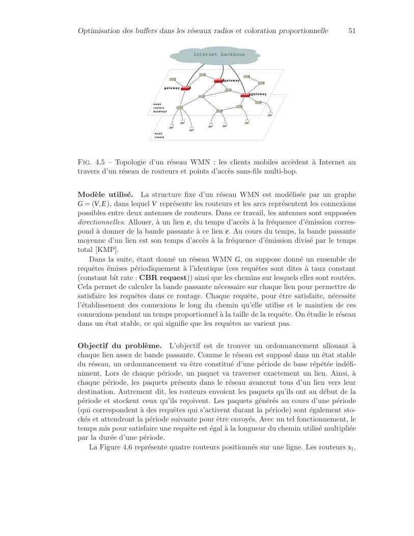
Optimisation des buffers dans les réseaux radios et coloration proportionnelle 51
Fig. 4.5 – Topologie d’un réseau WMN : les clients mobiles accèdent à Internet autravers d’un réseau de routeurs et points d’accès sans-fils multi-hop.
Modèle utilisé. La structure fixe d’un réseau WMN est modélisée par un grapheG = (V,E), dans lequel V représente les routeurs et les arcs représentent les connexionspossibles entre deux antennes de routeurs. Dans ce travail, les antennes sont supposéesdirectionnelles. Allouer, à un lien e, du temps d’accès à la fréquence d’émission corres-pond à donner de la bande passante à ce lien e. Au cours du temps, la bande passantemoyenne d’un lien est son temps d’accès à la fréquence d’émission divisé par le tempstotal [KMP].
Dans la suite, étant donné un réseau WMN G, on suppose donné un ensemble derequêtes émises périodiquement à l’identique (ces requêtes sont dites à taux constant(constant bit rate : CBR request)) ainsi que les chemins sur lesquels elles sont routées.Cela permet de calculer la bande passante nécessaire sur chaque lien pour permettre desatisfaire les requêtes dans ce routage. Chaque requête, pour être satisfaite, nécessitel’établissement des connexions le long du chemin qu’elle utilise et le maintien de cesconnexions pendant un temps proportionnel à la taille de la requête. On étudie le réseaudans un état stable, ce qui signifie que les requêtes ne varient pas.
Objectif du problème. L’objectif est de trouver un ordonnancement allouant àchaque lien assez de bande passante. Comme le réseau est supposé dans un état stabledu réseau, un ordonnancement va être constitué d’une période de base répétée indéfi-niment. Lors de chaque période, un paquet va traverser exactement un lien. Ainsi, àchaque période, les paquets présents dans le réseau avancent tous d’un lien vers leurdestination. Autrement dit, les routeurs envoient les paquets qu’ils ont au début de lapériode et stockent ceux qu’ils reçoivent. Les paquets générés au cours d’une période(qui correspondent à des requêtes qui s’activent durant la période) sont également sto-ckés et attendront la période suivante pour être envoyés. Avec un tel fonctionnement, letemps mis pour satisfaire une requête est égal à la longueur du chemin utilisé multipliéepar la durée d’une période.
La Figure 4.6 représente quatre routeurs positionnés sur une ligne. Les routeurs s1,
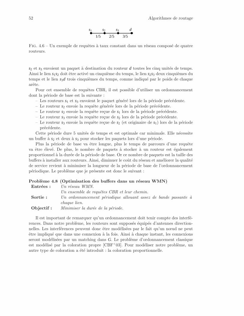
52 Algorithmes de routage
3/52/51/5
s1 s2 s3 d
Fig. 4.6 – Un exemple de requêtes à taux constant dans un réseau composé de quatrerouteurs.
s2 et s3 envoient un paquet à destination du routeur d toutes les cinq unités de temps.Ainsi le lien s1s2 doit être activé un cinquième du temps, le lien s2s3 deux cinquièmes dutemps et le lien s3d trois cinquièmes du temps, comme indiqué par le poids de chaquearête.
Pour cet ensemble de requêtes CBR, il est possible d’utiliser un ordonnancementdont la période de base est la suivante :
– Les routeurs s1 et s3 envoient le paquet généré lors de la période précédente.– Le routeur s2 envoie la requête générée lors de la période précédente.– Le routeur s2 envoie la requête reçue de s1 lors de la période précédente.– Le routeur s3 envoie la requête reçue de s2 lors de la période précédente.– Le routeur s3 envoie la requête reçue de s2 (et originaire de s1) lors de la période
précédente.Cette période dure 5 unités de temps et est optimale car minimale. Elle nécessite
un buffer à s2 et deux à s3 pour stocker les paquets lors d’une période.Plus la période de base va être longue, plus le temps de parcours d’une requête
va être élevé. De plus, le nombre de paquets à stocker à un routeur est égalementproportionnel à la durée de la période de base. Or ce nombre de paquets est la taille desbuffers à installer aux routeurs. Ainsi, diminuer le coût du réseau et améliorer la qualitéde service revient à minimiser la longueur de la période de base de l’ordonnancementpériodique. Le problème que je présente est donc le suivant :
Problème 4.8 (Optimisation des buffers dans un réseau WMN)Entrées : Un réseau WMN.
Un ensemble de requêtes CBR et leur chemin.Sortie : Un ordonnancement périodique allouant assez de bande passante à
chaque lien.Objectif : Minimiser la durée de la période.
Il est important de remarquer qu’un ordonnancement doit tenir compte des interfé-rences. Dans notre problème, les routeurs sont supposés équipés d’antennes direction-nelles. Les interférences peuvent donc être modélisées par le fait qu’un nœud ne peutêtre impliqué que dans une connexion à la fois. Ainsi à chaque instant, les connexionsseront modélisées par un matching dans G. Le problème d’ordonnancement classiqueest modélisé par la coloration propre [CBF+03]. Pour modéliser notre problème, unautre type de coloration a été introduit : la coloration proportionnelle.
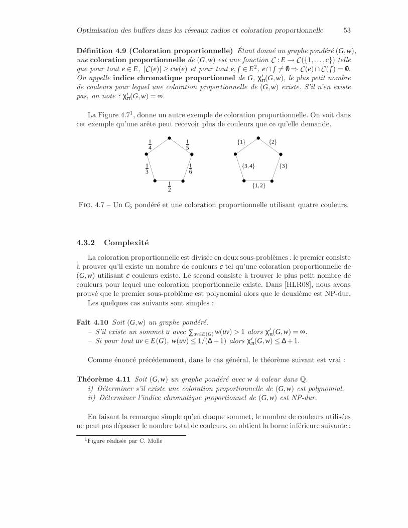
Optimisation des buffers dans les réseaux radios et coloration proportionnelle 53
Définition 4.9 (Coloration proportionnelle) Étant donné un graphe pondéré (G,w),une coloration proportionnelle de (G,w) est une fonction C : E → C (1, . . . ,c) telleque pour tout e∈ E, |C (e)| ≥ cw(e) et pour tout e, f ∈ E2, e∩ f 6= /0 ⇒ C (e)∩C ( f ) = /0.On appelle indice chromatique proportionnel de G, χ′
π(G,w), le plus petit nombrede couleurs pour lequel une coloration proportionnelle de (G,w) existe. S’il n’en existepas, on note : χ′
π(G,w) = ∞.
La Figure 4.71, donne un autre exemple de coloration proportionnelle. On voit danscet exemple qu’une arête peut recevoir plus de couleurs que ce qu’elle demande.
1,2
3,4
1 2
3
14
16
13
12
15
15
2
13
3,4 163
12
1,2
141
Fig. 4.7 – Un C5 pondéré et une coloration proportionnelle utilisant quatre couleurs.
4.3.2 Complexité
La coloration proportionnelle est divisée en deux sous-problèmes : le premier consisteà prouver qu’il existe un nombre de couleurs c tel qu’une coloration proportionnelle de(G,w) utilisant c couleurs existe. Le second consiste à trouver le plus petit nombre decouleurs pour lequel une coloration proportionnelle existe. Dans [HLR08], nous avonsprouvé que le premier sous-problème est polynomial alors que le deuxième est NP-dur.
Les quelques cas suivants sont simples :
Fait 4.10 Soit (G,w) un graphe pondéré.– S’il existe un sommet u avec ∑uv∈E(G) w(uv) > 1 alors χ′
π(G,w) = ∞.– Si pour tout uv∈ E(G), w(uv) ≤ 1/(∆ +1) alors χ′
π(G,w) ≤ ∆ +1.
Comme énoncé précédemment, dans le cas général, le théorème suivant est vrai :
Théorème 4.11 Soit (G,w) un graphe pondéré avec w à valeur dans Q.i) Déterminer s’il existe une coloration proportionnelle de (G,w) est polynomial.ii) Déterminer l’indice chromatique proportionnel de (G,w) est NP-dur.
En faisant la remarque simple qu’en chaque sommet, le nombre de couleurs utiliséesne peut pas dépasser le nombre total de couleurs, on obtient la borne inférieure suivante :
1Figure réalisée par C. Molle

54 Algorithmes de routage
Théorème 4.12 (Borne inférieure) Soit m le plus petit entier vérifiant les équationssuivantes :
∑v st uv∈E
⌈mw(uv)⌉ ≤ m (4.1)
On a m≤ χπ(G,w)
Dans [HLR08], nous montrons également comment utiliser la coloration fraction-naire pour obtenir une borne supérieure sur l’indice chromatique proportionnel. Nousmontrons aussi que pour certaines classes de graphes, dont les bipartis (Théorème 4.13),le problème devient polynomial.
Théorème 4.13 Soit (G,w) un graphe pondéré biparti. S’il existe une solution m auxéquations (4.1), alors (G,w) accepte une coloration proportionnelle utilisant m couleurs.
Remarques finales. Le problème d’ordonnancement qui a motivé l’introduction dela coloration proportionnelle laisse d’autres questions ouvertes. En effet, il serait inté-ressant de trouver des algorithmes d’approximations pour certaines classes de graphesqui apparaissent en télécommunications telles que les grilles triangulaires. Avec JosephYu, nous nous intéressons à la version de la coloration proportionnelle dans laquelle lesarêtes ayant la même couleur forment un matching induit, c.à.d. qu’il n’y a pas d’arêteentre deux arêtes de même couleur. Ce type de coloration modélise les interférencesentre des antennes non directionnelles.
4.4 Conclusion et Perspectives
Dans cette section, j’ai présenté trois problèmes différents concernant le routage derequêtes à l’intérieur d’un réseau. Pour chacun de ces problèmes, les caractéristiques duréseau sont utilisées pour avoir une approche théorique efficace. Le travail effectué surles deux premiers types de réseaux a abouti à des algorithmes de routage permettantde garantir un écart maximum par rapport à la solution optimale. Dans la troisièmesection, j’ai présenté des résultats concernant la complexité d’un problème d’optimisa-tion de l’ordonnancement des requêtes dans un réseau WiFi. Il reste encore à trouverdes algorithmes d’approximation pour ce dernier problème.

Chapitre 5
Réseaux d’accès et de cœur
Dans ce chapitre, je m’intéresse aux requêtes multicasts dans les réseaux op-tiques. J’y présente la technologie utilisée dans un réseau tout optique. Ensuite,je m’intéresse au dimensionnement d’un tel réseau. Ce problème est modélisé parun problème de coloration des graphes orientés et je présente les résultats obte-nus sur un problème de coloration des graphes orientés qui y est lié : le directedstar colouring (dst), entre autres, pour tout graphe orienté D, dst(D) ≤ 2∆− + 1et dst(D) ≤ 2max(∆+(D),∆−(D)). Ces résultats permettent d’estimer le gain induitpar l’utilisation de multicasts au lieu d’unicasts. Enfin, j’étudie des problèmes deroutage des multicasts dans les réseaux WDM d’accès et de cœur, pour lesquels jepropose plusieurs formulations mathématiques.
Le travail que je présente dans ce chapitre a été réalisé dans le cadre des réseauxoptiques mais il peut être généralisé à d’autre types de réseaux tels que les réseauxWiFi. Je présente différents problèmes de routage, ce chapitre concerne donc la couche3 (réseau) si l’on se réfère au système OSI. Je m’intéresse à des variantes du problèmede routage et d’affectation de longueurs d’onde, Problème 5.1. Il s’agit donc d’établiret de maintenir un ensemble de connexions pour satisfaire des requêtes données.
Je commence par présenter les technologies que je considère équipant les réseauxque j’étudie. Ensuite, je m’intéresse au problème du calcul du gain occasionné parl’utilisation de requêtes multicasts à la place de requêtes unicast. Pour cela, je présenteune modélisation permettant de ramener ce problème à un problème de coloration degraphe orienté. Je présente de nombreuses avancées concernant cette coloration. Dansla section suivante, je m’intéresse au problème de routage de multicasts proprement dit.Je présente plusieurs formulations pour ce problème, certaines adaptées aux réseaux decœurs, d’autres aux réseaux d’accès ; un réseau de coeur sert à interconnecter plusieursréseaux, les données y transitent assemblées sous forme de paquets et à haut débits pardes routes réservées (en utilisant des protocoles de type MPLS -Multiprotocol Label
55
56 Réseaux d’accès et de cœur
Switching-), tandis qu’un réseau d’accès sert à relier directement les utilisateurs auréseau de cœur et a souvent une faible conenctivité (voir Section 5.2.6 pour plus dedétails). Je ne fais pas d’hypothèse sur la structure des réseaux de cœur.
5.1 Introduction sur les réseaux optiques
Dans cette première section, je décris brièvement le fonctionnement d’un réseauoptique et le matériel disponible aujourd’hui. Je me suis entre autres basé sur [Alw04,Cor03] et la thèse de D. Coudert [Cou01], ainsi que celle de A. Guitton [Gui05]. Je meplace dans le cadre de l’optique guidée, en opposition à l’optique libre.
5.1.1 Technologies optiques
De manière générale, les données sont codées par des bits, c.à.d. des 0 et des 1. Dansun circuit électrique, une technique consiste à représenter le bit 1 par une tension nonnulle et le bit 0 par une tension nulle (dans d’autres codages, le bit 0 est représenté parune tension négative). En optique, le principe est le même, le bit 1 est codé par uneimpulsion lumineuse et le bit 0 par une absence de lumière. La durée de l’impulsionlumineuse dépend du débit de transmission, ainsi à un débit de 10 Gbits/s, étant donnéque la vitesse de la lumière est d’environ 300 000 km/s, un bit est codé par un segmentdont la longueur est environ 3 cm. Cette hypothèse est par exemple utilisée dans [Siu03].
5.1.1.1 Fibres optiques
Une fibre optique est composée d’un cœur en verre ou en plastique au sein du-quel se propage la lumière. Le phénomène physique permettant cette propagation estla réflexion de la lumière. En effet, si l’angle que fait le rayon lumineux avec la paroide la fibre (appelé angle d’incidence) n’est pas trop grand, alors la paroi se com-porte comme un miroir et le rayon est totalement réfléchi, voir Figure 5.1. On peutdonc considérer qu’une fibre optique se comporte comme un tuyau transmettant uneimpulsion lumineuse d’une extrémité à une autre. Il existe plusieurs types de fibres.Par exemple, les fibres multi-modes permettent la transmission simultanée de plusieursrayons lumineux ayant des angles d’incidence différents. Ce procédé provoque cepen-dant des interférences et je ne vais pas le considérer par la suite, je considère donc queles rayons lumineux ne se différencient pas par leur angle d’incidence, ceci est le casdans les fibres mono-mode. A la place, je considère un autre type de multiplexage : lemultiplexage en longueur d’onde que je présente dans la Section 5.1.1.5.
Outre le fait de permettre des transmissions très rapides (à une vitesse de l’ordre dela vitesse de la lumière), la communication optique présente de nombreux avantages.En effet, une transmission optique est insensible au bruit électromagnétique, elle induitune faible distorsion du signal et elle ne s’atténue que peu sur de longues distances (de0,2 à 1 dB/km sur les longueurs d’onde utilisées, voir Figure 5.21), il faut tout de mêmeutiliser des amplificateurs (c.f. Section 5.1.1.4). L’atténuation est en partie due à des
1Source : [Alw04]

Introduction sur les réseaux optiques 57
Indice de réfraction n2
Indice de réfraction n1
Fig. 5.1 – Principe de transmission dans une fibre optique.
impuretés dans le verre utilisé pour fabriquer la fibre. Les longueurs d’onde utiliséespour transmettre les données s’étalent de 800 à 1600 nanomètres, les plus utilisées sont850 nm, 1310 nm et 1550 nm ; la lumière visible s’étale quant à elle de 400 à 700 nm.
Enfin, les fibres optiques sont économiques en matière d’énergie utilisée et ne coûtentpas très cher.
Fig. 5.2 – Atténuation du signal lumineux dans une fibre optique.
5.1.1.2 Émetteurs
En dehors du réseau, les données existent sous forme électromagnétique. Les impul-sions lumineuses monochromatiques permettant de coder les informations sont injectéesdans la fibre optique à l’aide de diodes laser. Ce sont les caractéristiques de la diodelaser utilisée qui définissent la longueur d’onde sur laquelle l’impulsion lumineuse estémise.
Il y a de nombreux types de diodes laser. Je ne cite que les VCSEL (Vertical CavitySurface Emitting Laser) qui sont des lasers émettant perpendiculairement à la surfaceet qui sont utilisées pour les applications de communication par fibre optique à courte
58 Réseaux d’accès et de cœur
portée telles que le protocole Gigabit Ethernet. Les diodes VCSEL présentent l’avantaged’être plus facile à fabriquer et peuvent être disposées en matrices. Ces diodes sontégalement utilisées pour les réseaux en espace optique libre, réseaux dont il est questiondans la thèse de D. Coudert [Cou01].
5.1.1.3 Récepteurs
A une extrémité de la fibre se trouvent les diodes laser et à l’autre se trouventles récepteurs. Leur rôle est de transformer une impulsion lumineuse en une impulsionélectrique. Il est possible de faire cela avec des diodes photosensibles, leur fonction étantde convertir de la lumière en courant électrique. Le courant induit est ensuite amplifiéet soumis à un test de seuil pour savoir quel bit (0 ou 1) il code.
5.1.1.4 Amplificateurs
Au cours de sa transmission dans une fibre optique, un signal s’atténue, le phéno-mène correspondant est appelé la dispersion Rayleigh. On considère généralement quel’atténuation est de 0.2 dB par kilomètre et il est communément admis qu’un signalpeut être correctement interprété tant qu’il a été atténué de moins de 20 dB. Ainsi,pour permettre des transmissions sur de longues distances, il est nécessaire de réémettrele signal environ tous les 100 km. L’inconvénient de réémettre le signal est que cela in-duit un délai supplémentaire car il faut faire une conversion opto-électronique avantde le réémettre. Il existe une autre solution qui consiste à utiliser des amplificateursoptiques. Ce sont des dispositifs permettant d’amplifier un signal lumineux sans à avoirà le convertir en signal électrique. Il existe plusieurs types d’amplificateurs optiquesdont les amplificateurs à fibres dopées et les amplificateurs à effet Raman.
L’amplification optique a cependant des limites, en effet, à chaque amplification,du bruit est ajouté au signal, il faut donc, au bout d’un certain temps, réémettre lesignal. Les amplificateurs à effet Raman induisent moins de bruit que les amplificateursà fibres dopées.
En plus d’atténuer les impulsions lumineuses, la dispersion Rayleigh les déforme.La Figure 5.32 illustre un signal optique lors de son émission et après sa transmissionpar une fibre optique. Pour permettre une bonne réception il est donc nécessaire deremodeler les impulsions lumineuses.
Un troisième problème dont il faut tenir compte est la désynchronisation des si-gnaux. En effet, la vitesse de propagation d’un signal lumineux dépend de sa longueurd’onde et de son angle d’incidence. Pour garantir que le délai entre deux impulsionslumineuses censées arriver simultanément reste raisonnable, il est nécessaire de les re-synchroniser régulièrement.
La déformation et la désynchronisation des signaux ne sont pas critiques par rapportà l’atténuation et il est suffisant de remodeler et de synchroniser un signal tous les 500km. Il est donc possible de combiner cela avec la réémission rendue nécessaire parl’amplification du bruit lors de l’amplification du signal.
2inspirée de [Gui05]

Introduction sur les réseaux optiques 59
temps temps
fibre optique
inte
nsi
té
atténuation
dispersion
désynchronisation
Fig. 5.3 – Atténuation, déformation et désynchronisation des signaux lumineux.
5.1.1.5 Multiplexage
Le multiplexage est la capacité à transmettre sur un seul support (dans notre casla fibre optique) des données provenant de plusieurs sources. Il existe plusieurs typesde multiplexages, ici j’en présente deux.
Multiplexage temporel. Il s’agit d’allouer le temps d’utilisation de la fibre optiqueentre les différentes sources qui ont des données à transmettre. Ainsi l’accès à la fibreoptique est partagé en intervalles de temps qui sont répartis à chacune des sources, c.f.Figure 5.4.
Source 1
Source 2
Source 3
Fig. 5.4 – Multiplexage temporel.
Multiplexage en longueur d’onde. Dans le cas du multiplexage en longueur d’onde(Wavelength Division Multiplexing) WDM, les données sont émises dans la fibre op-tique sur différentes longueurs d’onde. Le multiplexage en longueur d’onde nécessitel’usage d’un multiplexeur en entrée, pour réunir les longueurs d’onde à transmettreen un seul signal lumineux, et d’un démultiplexeur en sortie, pour les dissocier, c.f.Figure 5.5.
Dans le cas des réseaux tout optique, les multiplexeurs/démultiplexeurs peuventêtre des prismes. Un réseau permettant le multiplexage en longueurs d’onde est équipé
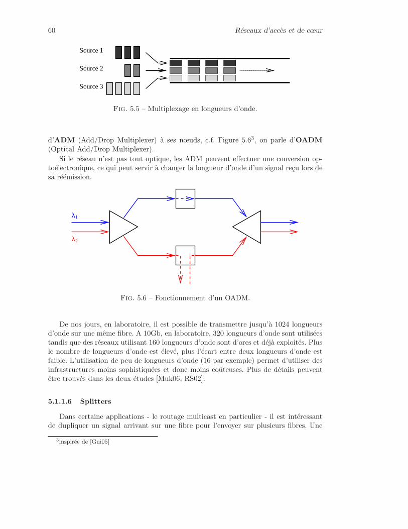
60 Réseaux d’accès et de cœur
Source 1
Source 2
Source 3
Fig. 5.5 – Multiplexage en longueurs d’onde.
d’ADM (Add/Drop Multiplexer) à ses nœuds, c.f. Figure 5.63, on parle d’OADM(Optical Add/Drop Multiplexer).
Si le réseau n’est pas tout optique, les ADM peuvent effectuer une conversion op-toélectronique, ce qui peut servir à changer la longueur d’onde d’un signal reçu lors desa réémission.
λ2
λ1
Fig. 5.6 – Fonctionnement d’un OADM.
De nos jours, en laboratoire, il est possible de transmettre jusqu’à 1024 longueursd’onde sur une même fibre. A 10Gb, en laboratoire, 320 longueurs d’onde sont utiliséestandis que des réseaux utilisant 160 longueurs d’onde sont d’ores et déjà exploités. Plusle nombre de longueurs d’onde est élevé, plus l’écart entre deux longueurs d’onde estfaible. L’utilisation de peu de longueurs d’onde (16 par exemple) permet d’utiliser desinfrastructures moins sophistiquées et donc moins coûteuses. Plus de détails peuventêtre trouvés dans les deux études [Muk06, RS02].
5.1.1.6 Splitters
Dans certaine applications - le routage multicast en particulier - il est intéressantde dupliquer un signal arrivant sur une fibre pour l’envoyer sur plusieurs fibres. Une
3inspirée de [Gui05]
Introduction sur les réseaux optiques 61
solution consiste à convertir le signal arrivant en un signal électrique et de le réémettresur les fibres sortantes. Pour éviter cette conversion, il est possible d’utiliser des splitters.
Les splitters que je considère dans les Sections 5.2.2 et 5.2.6 sont des composantsoptiques passifs. Ils reçoivent un signal en entrée sur une fibre donnée et divisent cesignal sur plusieurs fibres en sortie. Dans ce type de splitters, tous les signaux de toutesles longueurs d’onde de la fibre d’entrée sont divisés sur les fibres de sortie. On appellele nombre de fibres de sorties la taille du splitter. Un splitter de taille k est appelé un1 : k splitter. La puissance du signal d’entrée est répartie sur les différentes fibres desorties, on considère qu’un splitter 1 : 2 induit une atténuation de 3 à 3,5 dB. Dansla Section 5.2.1, je considère des splitters plus performants permettant de sélectionnerles longueurs d’onde dupliquées. J’appelle de tels splitters des splitters en longueursd’onde.
5.1.2 Modélisation d’un réseau optique WDM
Un réseau optique WDM est représenté par un graphe orienté D = (V,E). A chaquerouteur (ou système) du réseau physique est associé un sommet du graphe V = v1,v2, . . . ,vn.De manière similaire, chaque fibre optique du réseau est associée à un arc du grapheorienté E = e1,e2, . . . ,em. La capacité de chaque arc représente le nombre de longueursd’onde disponibles. En effet, on fait l’hypothèse simplificatrice que toutes les longueursd’onde ont la même capacité et que les requêtes sont routées seules sur une longueurd’onde (c.à.d. qu’il n’y a pas de groupage, c.f. Section 6.2.1), sauf si le contraire estspécifié.
Les connexions et les fibres optiques sont supposées orientées et le trafic asymétrique.Le trafic est composé d’un ensemble de requêtes qui sont caractérisées par leur sourceet leur destination. L’objectif est d’établir des connexions pour ces requêtes et de lesmaintenir. L’ensemble des longueurs d’onde disponibles dans le réseau est noté Λ =λ1,λ2, . . . ,λW avec W = |Λ|.
Dans ce contexte, le problème de routage présenté dans la Section 2.2.2 se com-plexifie. En effet, en plus de trouver un ensemble de chemins pour les requêtes, il fautégalement assigner à chaque chemin une longueur d’onde. Excepté dans la Section 6.2,je fais l’hypothèse de continuité en longueur d’onde, autrement dit les données sonttransmises par un signal lumineux dont la longueur d’onde ne varie pas le long duchemin. Le problème de routage peut être présenté comme suit :
Problème 5.1 (Problème de routage et d’affectation de longueurs d’onde(RWA))
Entrées : Un réseau optique WDM.Un ensemble de requêtes.
Sorties : Un chemin réalisable pour chaque requête.Une longueur d’onde associée à chaque chemin de telle sorte qu’aucunchemin utilisant une même arête n’ait la même longueur d’onde.
Objectif : Minimiser le coût du routage.

62 Réseaux d’accès et de cœur
5.2 Multicast
Dû au développement des applications multi-utilisateurs, telles que la télévisionhaute définition ou sur Internet, les vidéoconférences, les applications à la demandeet les jeux en réseau, il est crucial d’économiser le plus possible de bande passante enne transmettant pas de données redondantes. C’est pour cette raison que de plus enplus d’attention se porte sur les requêtes ayant une source et plusieurs destinations. Onappelle de telles requêtes des requêtes multicasts, une requête ayant une source et uneseule destination est, elle, appelée requête unicast. Par abus de langage, j’appelle unerequête multicast un multicast. A l’heure actuelle, les multicasts sont le plus souventeffectués sous la forme d’autant de requêtes unicast (une source, une destination) qu’ilsont de destinations. Cette technique, appelée multi-unicast, encombre à la fois lasource et le réseau. L’intérêt du véritable multicast est de permettre d’économiser de labande passante sur une partie du chemin à parcourir (les sections de routage communes)et de permettre à la source de ne pas réémettre plusieurs fois le même message. Eneffet, il suffit d’envoyer le message sur une longueur d’onde et de le dupliquer à l’aided’un splitter là où c’est nécessaire (c.à.d. à chaque point de séparation des routes àemprunter) pour atteindre chacune des destinations. L’utilisation de splitters permetdonc d’étendre les possibilités de routage en permettant, en plus de l’utilisation dechemins, l’utilisation d’arbres pour router les requêtes. Un lecteur intéressé peut seréférer aux articles [MZQ98, SM99] pour plus de détails sur les apports du multicast,ainsi qu’à la thèse de A. Guitton : Communications multicast [Gui05].
Déploiement du multicast. Comme dans le cas du routage des unicasts, il estnécessaire de décrire le routage et l’adressage des paquets. Pour les unicasts, ce problèmeest résolu de manière efficace. Pour les multicasts, afin de décrire l’adressage et leroutage des paquets, c’est le modèle proposé par Deering dans [Dee91] qui a été adoptépar l’organisme de standardisation de l’IETF. Dans sa thèse, A. Guitton, présentece modèle ainsi que ses limites. Il présente et compare d’autre protocoles dont lesprotocoles Xcast [BFI+07], Xcast+ [SKPK01], GXcast [BGC04] et Linkcast.
Les protocoles cités précédemment nécessitent l’interprétation des en-têtes des pa-quets transmis, or cela n’est pas réalisable dans un réseau tout optique très haut débit.Dans ce chapitre, j’envisage donc le cas où le routage est fait physiquement.
Objectifs. Il est important de pouvoir implémenter un routage de multicasts efficacetant en termes de bande passante utilisée que de coût d’infrastructure. En effet, l’ins-tallation de splitters induit un surcoût au réseau. Cela mène à l’étude de plusieurs pro-blèmes dont le problème de Dimensionnement de Réseaux et le problème Routagede Multicasts et Affectation de Longueurs d’Ondes (MultiCast WavelengthRouting and Assignment) MC-RWA. Deux surveys sont disponibles sur ce dernierproblème : [HCT02] et [Rou03] qui est une extension du Problème 5.1.

Multicast 63
Problème 5.2 (Dimensionnement de réseau)Entrée : Caractéristiques des requêtes à router.Sortie : Caractéristiques suffisantes du réseau.Objectif : Minimiser le coût du réseau.
Problème 5.3 (Routage de Multicasts et Affectation de Longueursd’Ondes : MC-RWA)
Entrées : Un réseau avec des coûts et des capacités sur les liens.Un ensemble de requêtes multicasts.
Sortie : Un routage (arbres et longueur d’onde) des requêtes multicasts.Objectif : Minimiser le coût.
Plan. De nos jours, il existe des splitters en longueurs d’onde mais ils ne sont pasencore utilisés dans les réseaux existants ou, si ils le sont, ils le sont de manière anec-dotique. Dans la Section 5.2.1, j’étudie le problème 5.2 en évaluant l’impact qu’auraitl’utilisation des splitters en longueurs d’onde. Nous y étudions le nombre de longueursd’onde nécessaire au routage des multicasts en fonction de leur nombre et du nombrede destinataires. Cela permet de quantifier l’économie induite par l’installation d’unsplitter en longueurs d’onde.
Par la suite, dans les Sections 5.2.2 et 5.2.6, je m’intéresse au Problème 5.3 MC-RWAdans des réseaux réels. Ainsi je ne considère que les splitters dupliquant l’intégralitéd’une fibre, tels qu’ils sont décrits dans la Section 5.1.1.6. Cette hypothèse a très peu étéprise en compte car elle est très contraignante, elle semble pourtant bien plus réalisted’après les contacts que nous avons eus avec Nicolas Gagnon de NORTEL Networks -EXFO. Dans la Section 5.2.2, je décris plusieurs formulations mathématiques permet-tant de résoudre MC-RWA dans un réseau optique de cœur. Je considére l’objectif deminimiser le nombre de requêtes rejetées puis celui de minimiser le nombre d’utilsateursnon satisfaits. Dans la Section 5.2.6, je m’intéresse à MC-RWA dans les réseaux d’accès,l’objectif de cette section étant de prendre en compte les caractéristiques des réseauxd’accès pour pouvoir améliorer le temps de résolution.
5.2.1 Dimensionnement d’un réseau en étoile
Cette section concerne un travail soumis à Combinatorics, Probability and Compu-ting, réalisé avec O. Amini, F. Havet et S. Thomassé sur un réseau bien particulier :un réseau en étoile. L’article soumis peut être trouvé dans l’Annexe C.1.
Un réseau en étoile est un réseau composé de plusieurs systèmes, par exemple desordinateurs, tous reliés à un nœud central par le même nombre de fibres optiques. Onnote l’ensemble des systèmes V et le nombre de fibres n, ces informations caractérisentnotre réseau. On suppose de plus que le réseau est un réseau WDM, c’est-à-dire queles transmissions se font sur différentes longueurs d’onde à l’intérieur d’une même fibre(Section 5.1.1.5). Enfin, on suppose que le nœud central est un transmetteur toutoptique qui peut renvoyer sur un ensemble de fibres un message reçu mais qui ne peutpas en modifier la longueur d’onde. Autrement dit, le nœud central est un splitter

64 Réseaux d’accès et de cœur
capable de dupliquer un signal optique sans en modifier la longueur d’onde (Section5.1.1.6).
Nous nous sommes intéressés au dimensionnement d’un tel réseau. Les entrées denotre problème sont le nombre de fibres reliant chaque système au nœud central etun ensemble de contraintes sur les multicasts à router. Les contraintes peuvent portersur le nombre maximum de multicasts envoyés et reçus par chaque système ou encoresur le nombre de destinataires de chaque multicast. L’objectif est de trouver le nombreminimum de longueurs d’onde nécessaires pour assurer l’existence d’un routage pourtout ensemble de multicasts satisfaisant les contraintes que l’on s’est fixées.
Ces travaux s’effectuent dans la lignée de ceux réalisés par R. Brandt et T.F. Gon-zalez [BG05]. Une des conséquences de ce travail est de permettre de calculer l’impactd’un splitter en longueurs d’onde sur le coût d’un réseau. Cet impact sur le coût adéjà été évalué dans l’article [MZQ98]. Les auteurs y étudient également des réseauxéquipés de splitters en longueurs d’onde et ont une approche empirique. Nos travauxont également un fort intérêt théorique puisque nous avons grandement amélioré lesbornes supérieures sur le nombre maximum de couleurs nécessaires dans un problèmede coloration des graphes orientés.
Problème 5.4 (Dimensionnement d’un réseau en étoile)Entrées : Nombre de fibres.
Nombre de multicasts envoyés par un système.Nombre de multicasts reçus par un système.Nombre maximum de destinataires d’un multicast.
Sortie : Un nombre de longueurs d’onde suffisant pour router tout ensemblede requêtes envisagées.
Objectif : minimiser le nombre de longueurs d’onde.
Plan. Je présente en premier lieu les résultats dans le cas où chaque système est reliépar une seule fibre au nœud central et envoie au plus un multicast. Cette étude esteffectuée dans le cas où le nombre de multicasts reçus par chaque nœud est borné, puisquand pour un nœud donné la somme du nombre de multicasts reçus et envoyés estbornée, et enfin quand le nombre de multicasts reçus et le nombre de multicasts envoyéssont tous les deux bornés. Dans ces différents cas, le problème se ramène à l’étude d’unecoloration naturelle des graphes orientés. Dans la dernière section, je présente le casplus général où il y a plusieurs fibres reliant chaque système au nœud central et où lenombre maximum de multicasts envoyés par un même système est borné. Dans ce cas,le problème est une extension du problème de coloration précédent pour les graphesorientés labélisés.
5.2.1.1 Une fibre, un multicast
Dans cette section, je suppose que chaque système est relié par une unique fibre aunœud central et qu’il envoie un multicast M(v) à un ensemble de systèmes S(v) : M(v) =v,S(v). Trouver le nombre minimum de longueurs d’onde nécessaires au routage de
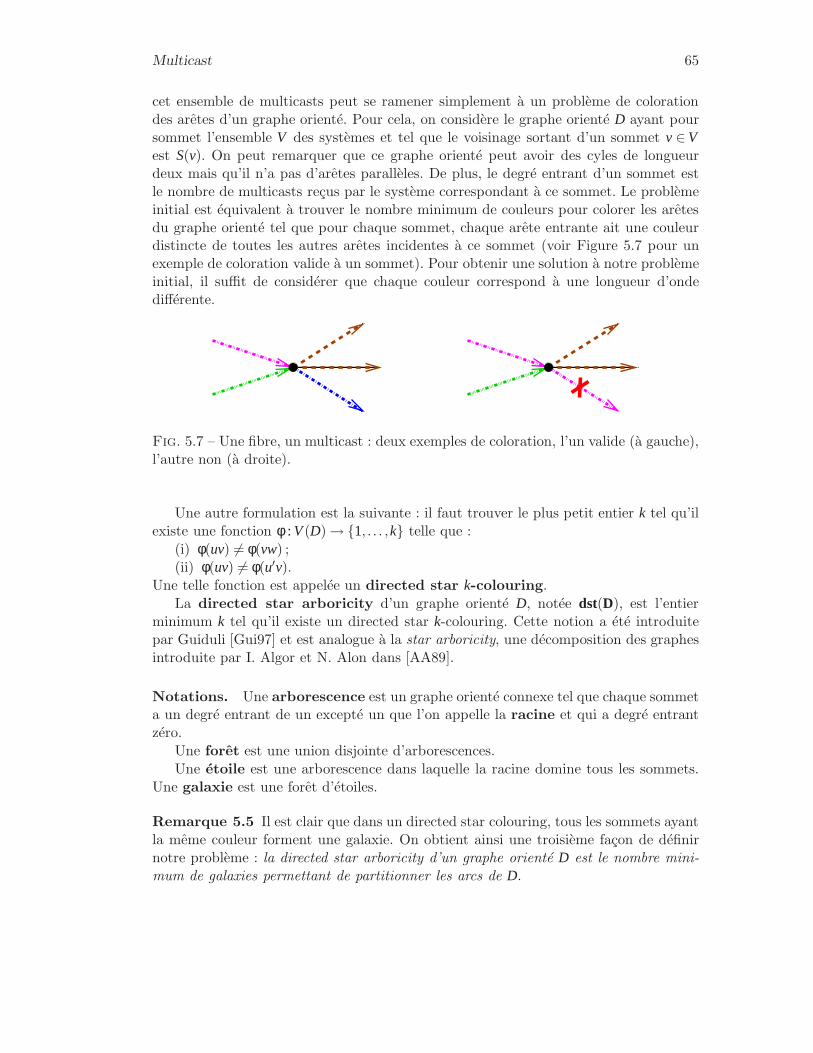
Multicast 65
cet ensemble de multicasts peut se ramener simplement à un problème de colorationdes arêtes d’un graphe orienté. Pour cela, on considère le graphe orienté D ayant poursommet l’ensemble V des systèmes et tel que le voisinage sortant d’un sommet v∈Vest S(v). On peut remarquer que ce graphe orienté peut avoir des cyles de longueurdeux mais qu’il n’a pas d’arêtes parallèles. De plus, le degré entrant d’un sommet estle nombre de multicasts reçus par le système correspondant à ce sommet. Le problèmeinitial est équivalent à trouver le nombre minimum de couleurs pour colorer les arêtesdu graphe orienté tel que pour chaque sommet, chaque arête entrante ait une couleurdistincte de toutes les autres arêtes incidentes à ce sommet (voir Figure 5.7 pour unexemple de coloration valide à un sommet). Pour obtenir une solution à notre problèmeinitial, il suffit de considérer que chaque couleur correspond à une longueur d’ondedifférente.
Fig. 5.7 – Une fibre, un multicast : deux exemples de coloration, l’un valide (à gauche),l’autre non (à droite).
Une autre formulation est la suivante : il faut trouver le plus petit entier k tel qu’ilexiste une fonction φ : V(D) →1, . . . ,k telle que :
(i) φ(uv) 6= φ(vw) ;(ii) φ(uv) 6= φ(u′v).
Une telle fonction est appelée un directed star k-colouring.La directed star arboricity d’un graphe orienté D, notée dst(D), est l’entier
minimum k tel qu’il existe un directed star k-colouring. Cette notion a été introduitepar Guiduli [Gui97] et est analogue à la star arboricity, une décomposition des graphesintroduite par I. Algor et N. Alon dans [AA89].
Notations. Une arborescence est un graphe orienté connexe tel que chaque sommeta un degré entrant de un excepté un que l’on appelle la racine et qui a degré entrantzéro.
Une forêt est une union disjointe d’arborescences.Une étoile est une arborescence dans laquelle la racine domine tous les sommets.
Une galaxie est une forêt d’étoiles.
Remarque 5.5 Il est clair que dans un directed star colouring, tous les sommets ayantla même couleur forment une galaxie. On obtient ainsi une troisième façon de définirnotre problème : la directed star arboricity d’un graphe orienté D est le nombre mini-mum de galaxies permettant de partitionner les arcs de D.

66 Réseaux d’accès et de cœur
Complexité. Dans [AHHT07], nous montrons que trouver la directed star arboricityd’un graphe orienté est un problème NP-dur. Nous le montrons en ramenant le problèmed’arêtes coloration des graphes cubique à notre problème dans le cas où le graphe orientéa un degré entrant et sortant d’au plus 2.
Cela implique que le problème suivant est NP-dur, alors même que le nombre delongueurs d’onde nécessaires est au plus cinq :
Problème 5.6 (Dimensionnement d’un réseau en étoile, complexité)Entrées : Chaque système est relié par une fibre au sommet central.
Chaque système est source d’au plus un multicast.Chaque système reçoit au plus deux multicasts.Chaque multicast est adressé à au plus deux systèmes.
Sortie : Nombre de longueurs d’onde nécessaires pour router un ensemble derequêtes.
Objectif : Minimiser le nombre de longueurs d’onde nécessaires.
Sachant ce résultat, il est intéressant de trouver des bornes supérieures sur le nombrede longueurs d’onde nécessaires dans le Problème 5.4 en fonction des différents para-mètres du problème. La section suivante s’intéresse au cas où le degré entrant est borné.
Degré entrant borné.
Problème 5.7 (Dimensionnement d’un réseau en étoile, degré entrantborné)
Entrées : Chaque système est relié par une fibre au sommet central.Chaque système est source d’au plus un multicast.Chaque système reçoit au plus k multicasts.
Sortie : Un nombre de longueurs d’onde suffisant pour router tout ensemblede requêtes envisagées.
Objectif : Minimiser le nombre de longueurs d’onde.
R. Brandt et T.F. Gonzalez [BG05] ont montré que dst(D) ≤ ⌈5∆−/2⌉. Dans le casoù ∆− = 1 cette borne est serrée car les circuits impairs ont une star arboricity de3. Cependant pour de plus grandes valeurs de ∆− il est possible de l’améliorer. Nousconjecturons que si ∆− ≥ 2, alors dst(D) ≤ 2∆−.
Conjecture 5.8 Tout graphe orienté D de degré entrant au plus ∆−≥ 2 vérifie dst(D)≤2∆−.
Cette conjecture serait serrée car Brandt [Bra03] montre que pour tout ∆−, il existeun graphe orienté acyclique D∆− de degré maximum ∆− et tel que dst(D∆−) = 2∆−.
On peut remarquer qu’afin de prouver cette conjecture, il est suffisant de la prouverpour ∆− = 2 et ∆− = 3. En effet, un graphe orienté de degré entrant maximum ∆− ≥ 2admet une partition de ses arêtes en ∆−/2 graphes orientés de degré entrant maximum2 si ∆− est pair et en (∆−−1)/2 graphes orientés de degré maximum 2 et un de degréentrant maximum 3 si ∆− est impair. Pour trouver cette partition, il suffit d’enlever augraphe orienté un sous-graphe eulérien maximum de manière récursive.
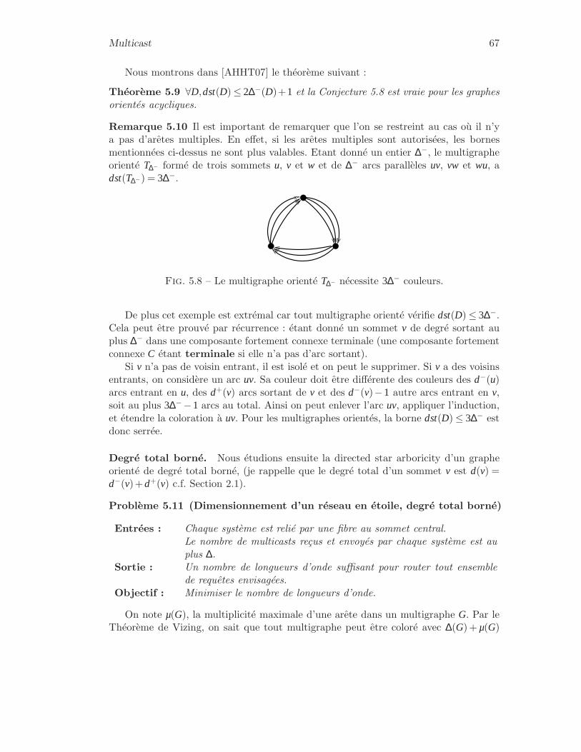
Multicast 67
Nous montrons dans [AHHT07] le théorème suivant :
Théorème 5.9 ∀D,dst(D)≤ 2∆−(D)+1 et la Conjecture 5.8 est vraie pour les graphesorientés acycliques.
Remarque 5.10 Il est important de remarquer que l’on se restreint au cas où il n’ya pas d’arêtes multiples. En effet, si les arêtes multiples sont autorisées, les bornesmentionnées ci-dessus ne sont plus valables. Etant donné un entier ∆−, le multigrapheorienté T∆− formé de trois sommets u, v et w et de ∆− arcs parallèles uv, vw et wu, adst(T∆−) = 3∆−.
Fig. 5.8 – Le multigraphe orienté T∆− nécessite 3∆− couleurs.
De plus cet exemple est extrémal car tout multigraphe orienté vérifie dst(D) ≤ 3∆−.Cela peut être prouvé par récurrence : étant donné un sommet v de degré sortant auplus ∆− dans une composante fortement connexe terminale (une composante fortementconnexe C étant terminale si elle n’a pas d’arc sortant).
Si v n’a pas de voisin entrant, il est isolé et on peut le supprimer. Si v a des voisinsentrants, on considère un arc uv. Sa couleur doit être différente des couleurs des d−(u)arcs entrant en u, des d+(v) arcs sortant de v et des d−(v)−1 autre arcs entrant en v,soit au plus 3∆−−1 arcs au total. Ainsi on peut enlever l’arc uv, appliquer l’induction,et étendre la coloration à uv. Pour les multigraphes orientés, la borne dst(D) ≤ 3∆− estdonc serrée.
Degré total borné. Nous étudions ensuite la directed star arboricity d’un grapheorienté de degré total borné, (je rappelle que le degré total d’un sommet v est d(v) =d−(v)+d+(v) c.f. Section 2.1).
Problème 5.11 (Dimensionnement d’un réseau en étoile, degré total borné)
Entrées : Chaque système est relié par une fibre au sommet central.Le nombre de multicasts reçus et envoyés par chaque système est auplus ∆.
Sortie : Un nombre de longueurs d’onde suffisant pour router tout ensemblede requêtes envisagées.
Objectif : Minimiser le nombre de longueurs d’onde.
On note µ(G), la multiplicité maximale d’une arête dans un multigraphe G. Par leThéorème de Vizing, on sait que tout multigraphe peut être coloré avec ∆(G)+ µ(G)

68 Réseaux d’accès et de cœur
couleurs de telle manière que toutes les arêtes incidentes aient deux couleurs différentes.Comme le multigraphe sous-jacent à un graphe orienté a une multiplicité d’au plus deux,tout graphe orienté D est tel que dst(D) ≤ ∆ +2.
Nous faisons la conjecture suivante :
Conjecture 5.12 Soit D un graphe orienté de degré maximum ∆≥ 3. On a dst(D)≤ ∆.
Cette conjecture serait serrée puisque tout graphe orienté ayant ∆ = ∆− a une stararboricity d’au moins ∆. Nous montrons dans [AHHT07] le théorème suivant :
Théorème 5.13 La conjecture 5.12 est vraie quand ∆ = 3.
Degré entrant et degré sortant borné. Une première approche pour résoudre lesConjectures 5.8 et 5.12 serait de les prouver dans le cas où les degrés entrant et sortantsont bornés.
Problème 5.14 (Dimensionnement d’un réseau en étoile, degré entrant etdegré sortant borné)
Entrées : Chaque système est relié par une fibre au sommet central.Chaque système est source d’au plus un multicast.Chaque système reçoit au plus k multicasts.Chaque multicast est adressé à au plus k systèmes.
Sortie : Un nombre de longueurs d’onde suffisant pour router tout ensemblede requêtes envisagées.
Objectif : Minimiser le nombre de longueurs d’onde.
Dans ce cadre là, on a les conjectures plus faibles suivantes :
Conjecture 5.15 Pour tout k≥ 2, et tout graphe orienté D, si max(∆−,∆+) ≤ k alorsdst(D) ≤ 2k.
Ces conjectures sont vraies et loin d’être serrées pour k grand. En effet, B. Gui-duli [Gui97] a montré que si max(∆−,∆+) ≤ k alors dst(D) ≤ k+20log(k)+84.
La preuve de B. Guiduli se base sur le fait que si les degrés entrant et sortant sontbornés, la coloration d’un arc ne dépend que des colorations d’un nombre limité d’autresarcs. Cette dépendance bornée permet d’utiliser le Lemme Local de Lovász. Cette idéea initialement été utilisée par I. Algor et N. Alon [AA89] pour la star arboricity desgraphes non orientés. On peut également remarquer que le résultat de Guiduli estpresque serré puisqu’il existe des graphes orientés D avec max(∆−,∆+) ≤ k et dst(D) ≥k+ Ω(log(k)) (voir [Gui97]).
Enfin, il est intéressant de remarquer que comme pour la Conjecture 5.8, il est suffi-sant de prouver la Conjecture 5.15 pour k = 2 et k = 3. Nous montrons dans [AHHT07]le théorème suivant :
Théorème 5.16 La Conjecture 5.15 est vraie pour k = 2, ce qui l’implique pour toutevaleur paire de k.
Il ne reste donc plus qu’à la prouver pour k = 3.

Multicast 69
Directed star arboricity acircuitique. A. Pinlou et É. Sopena [PS06] ont étu-dié une version plus forte de la directed star arboricity, appellée directed star arbori-city acircuitique. Il rajoute la condition que tout circuit doit avoir trois couleurs dis-tinctes. Cette notion ne s’applique qu’aux graphes orientés asymétriques, c’est-à-direaux graphes orientés sans circuit de longueur 2. En effet, un circuit de longueur 2 nepeut pas recevoir 3 couleurs. Les auteurs ont montré que la directed star arboricityacircuitique d’un graphe de degré maximum 3 est au plus 4. Dans [AHHT07], nousproposons une preuve plus courte de ce résultat.
5.2.1.2 Plusieurs fibres, plusieurs multicasts
Nous étudions, dans cette section, le cas plus général où le nœud central est reliéà chaque système par n fibres optiques et où chaque système peut envoyer plusieursmulticasts.
On note M1(v), . . . ,Ms(v)(v) les s(v) multicasts envoyés par un système v∈V. Pour1 ≤ i ≤ s(v), l’ensemble des nœuds destinataires du multicast Mi(v) est noté Si(v). Leproblème est toujours de trouver le nombre minimum de longueurs d’onde pour assurerl’existence d’un routage des multicasts.
Problème 5.17 (Dimensionnement d’un réseau en étoile multifibre)
Entrées : Chaque système est relié par n fibres au sommet central.Chaque système est source d’au plus m multicasts.Chaque système reçoit au plus k multicasts.
Sortie : Un nombre de longueurs d’onde suffisant pour router tout ensemblede requêtes envisagé.
Objectif : Minimiser le nombre de longueurs d’onde.
De nouveau, on peut modéliser ce problème par un problème de coloration d’ungraphe orienté, mais cette fois on a besoin d’un graphe orienté étiqueté.
Comme précédemment, on considère un graphe orienté ayant V comme ensemble desommets. Pour tout multicast Mi(v) = (v,Si(v)), v∈V, 1≤ i ≤ s(v), on ajoute l’ensembled’arcs Ai(v) = vw,w∈ Si(v) étiquetés i. L’étiquette d’un arc a est noté l(a).
On remarque que pour tout couple de sommets (u,v) et pour toute étiquette i il ya au plus un arc uv étiqueté i. Si le nombre maximum de multicasts envoyés par unsystème est m, alors il y a au plus m étiquettes différentes sur les arcs. Un tel grapheorienté est dit m-étiqueté.
Notre objectif est de trouver un n-fiber wavelength assignment de D, qui est unfonction Φ : A(D) → Λ×1, . . . ,n×1, . . .n qui associe tout arc uv à un triplet(λ(uv), f +(uv), f−(uv)) tel que :
(i) ∀uv,vw∈ E,(λ(uv), f−(uv)) 6= (λ(vw), f +(vw)) ;(ii) ∀uv,u′v∈ E,λ(uv), f−(uv)) 6= (λ(u′v), f−(u′v)) ;(iii) ∀vw,vw′ ∈ E, si l(vw) 6= l(vw′) alors (λ(vw), f +(vw)) 6= (λ(vw′), f +(vw′)).
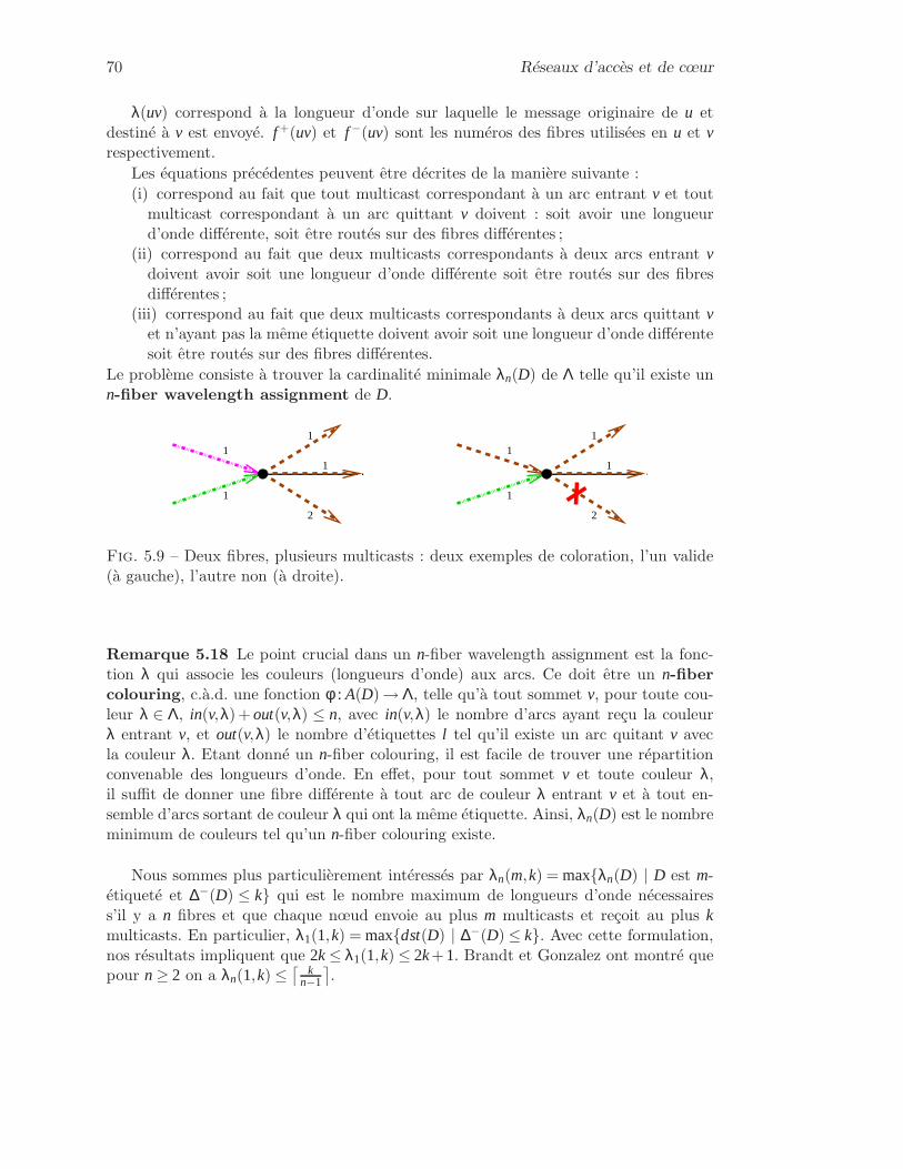
70 Réseaux d’accès et de cœur
λ(uv) correspond à la longueur d’onde sur laquelle le message originaire de u etdestiné à v est envoyé. f +(uv) et f−(uv) sont les numéros des fibres utilisées en u et vrespectivement.
Les équations précédentes peuvent être décrites de la manière suivante :(i) correspond au fait que tout multicast correspondant à un arc entrant v et tout
multicast correspondant à un arc quittant v doivent : soit avoir une longueurd’onde différente, soit être routés sur des fibres différentes ;
(ii) correspond au fait que deux multicasts correspondants à deux arcs entrant vdoivent avoir soit une longueur d’onde différente soit être routés sur des fibresdifférentes ;
(iii) correspond au fait que deux multicasts correspondants à deux arcs quittant vet n’ayant pas la même étiquette doivent avoir soit une longueur d’onde différentesoit être routés sur des fibres différentes.
Le problème consiste à trouver la cardinalité minimale λn(D) de Λ telle qu’il existe unn-fiber wavelength assignment de D.
1
2
1
1
11
2
1
1
1
Fig. 5.9 – Deux fibres, plusieurs multicasts : deux exemples de coloration, l’un valide(à gauche), l’autre non (à droite).
Remarque 5.18 Le point crucial dans un n-fiber wavelength assignment est la fonc-tion λ qui associe les couleurs (longueurs d’onde) aux arcs. Ce doit être un n-fibercolouring, c.à.d. une fonction φ : A(D)→ Λ, telle qu’à tout sommet v, pour toute cou-leur λ ∈ Λ, in(v,λ)+ out(v,λ) ≤ n, avec in(v,λ) le nombre d’arcs ayant reçu la couleurλ entrant v, et out(v,λ) le nombre d’étiquettes l tel qu’il existe un arc quitant v avecla couleur λ. Etant donné un n-fiber colouring, il est facile de trouver une répartitionconvenable des longueurs d’onde. En effet, pour tout sommet v et toute couleur λ,il suffit de donner une fibre différente à tout arc de couleur λ entrant v et à tout en-semble d’arcs sortant de couleur λ qui ont la même étiquette. Ainsi, λn(D) est le nombreminimum de couleurs tel qu’un n-fiber colouring existe.
Nous sommes plus particulièrement intéressés par λn(m,k) = maxλn(D) | D est m-étiqueté et ∆−(D) ≤ k qui est le nombre maximum de longueurs d’onde nécessairess’il y a n fibres et que chaque nœud envoie au plus m multicasts et reçoit au plus kmulticasts. En particulier, λ1(1,k) = maxdst(D) | ∆−(D) ≤ k. Avec cette formulation,nos résultats impliquent que 2k≤ λ1(1,k) ≤ 2k+1. Brandt et Gonzalez ont montré quepour n≥ 2 on a λn(1,k) ≤
⌈
kn−1
⌉
.
Multicast 71
n≥ 2 et m≥ 2. Nous montrons que si m≥ n alors il existe une constante C telle que :⌈
mn
⌈
kn
⌉
+kn
⌉
≤ λn(m,k) ≤⌈
mn
⌈
kn
⌉
+kn
⌉
+Cm2 log(k)
n
Nous conjecturons que la borne inférieure est la bonne valeur de λn(m,k) quand m≥ n.Nous montrons également que si m< n alors :
⌈
mn
⌈
kn
⌉
+kn
⌉
≤ λn(m,k) ≤⌈
kn−m
⌉
.
Les bornes inférieures généralisent les résultats de Brandt et Gonzalez [BG05] qui éta-blissaient ces inégalités dans le cas particulier k≤ 2, m≤ 2 et k= m. Les graphes orientésutilisés pour obtenir les bornes inférieures sont tous acycliques et nous montrons quesi m≥ n, alors les bornes inférieures donnent en effet la bonne valeur pour les graphesorientés acycliques. De plus, les graphes orientés atteignant les bornes inférieures ontun grand degré. En généralisant les résultats de Guiduli [Gui97], nous montrons qu’ungraphe orienté D m-étiqueté ayant son degré entrant et sortant borné par k peut êtrecoloré avec peu de couleurs :
λn(D) ≤ kn
+C′m2 log(k)
npour une constante C′.
5.2.1.3 Apport d’un splitter
A partir de l’analyse précédente, il est possible de quantifier l’apport d’un splitteren longueurs d’onde dans un réseau en étoile. Prenons un exemple pour fixer les idées :dans le cas où chaque système est relié par une fibre au nœud central, si on note k lenombre maximum de multicasts envoyés et reçus par un nœud du réseau, alors pourassurer l’existence d’un routage sans splitter, il faut 2k+1 longueurs d’onde par fibre.Avec un splitter en longueurs d’onde au nœud central il suffit de k+O(log(k)) longueursd’onde. Ainsi, un splitter en longueurs d’onde permet de diviser par deux le nombre delongueurs d’onde nécessaires.
Selon une remarque d’O. Amini, ce résultat peut se généraliser à un réseau quel-conque qui possède à chaque nœud des splitters capable de dupliquer chacune des lon-gueurs d’onde indépendamment. Le problème est, étant donné un routage de requêtes(c.à.d. un ensemble de chemins et d’arbres permettant de router chacune des requêtes),de savoir combien de longueurs d’onde sont nécessaires pour pouvoir le réaliser, autre-ment dit de savoir combien il faut de longueurs d’onde pour pouvoir en donner une àchacun des chemins et des arbres de telle sorte qu’il n’y ait pas de conflit. Dans le casoù le réseau est équipé de splitters, si le routage est tel que la profondeur de chaquearbre de routage est bornée et que le nombre maximum de feuilles de chaque arbre deroutage est borné par une constante fois la charge maximale du réseau ℓ, il suffit deℓ+O(log(ℓ)) longueurs d’onde. Dans le cas où le réseau n’est pas équipé de splitters, ilpeut falloir jusqu’a (∆ +1)ℓ longueurs d’onde où ∆ est le degré maximum du réseau.
Cela permet de déduire que l’utilisation de splitters en longueurs d’onde permetun gain théorique d’un facteur 1/(∆ + 1) concernant le nombre de longueurs d’onde
72 Réseaux d’accès et de cœur
nécessaires. D’autre part, équiper les nœuds de convertisseurs de longueurs d’ondepermet d’économiser de l’ordre de log(ℓ) longueurs d’onde.
Dans [MZQ98], les auteurs avaient estimés que l’utilisation de multicasts permetde réduire d’au moins 50 % le nombre de longueurs d’onde nécessaires. Ils montrentégalement que la conversion en longueur d’onde ne permet qu’un gain de l’ordre de 10%.
Ces résultats vont dans le même sens que nos résultats. En effet le gain théorique dela conversion en longueur d’onde est faible : de seulement un facteur additif de O(log(ℓ)),à comparé au gain empirique de 10 %. Si l’apport théorique semble plus faible que celuimesuré de manière empirique, cela est surement dû à l’utilisation d’algorithmes gloutonsdans [MZQ98].
Enfin, l’apport du multicast mis en évidence dans [MZQ98] est élevé (facteur 2) toutcomme dans notre étude. Il est cependant plus faible que l’apport théorique (facteur 3,2en moyenne pour leur instance utilisant NFSnet). Cela peut être expliqué par au moinsdeux raisons. La première est que les cas pour lesquels sont calculés le gain maximalthéorique sont pathologiques. La seconde raison est que les auteurs de [MZQ98], necalculent pas des routages optimaux.
5.2.2 Multicast dans les réseaux de cœur
Dans la section précédente, j’ai présenté les apports d’un splitter en longueurs d’ondepar rapport à l’absence de splitters. Dans la pratique, les réseaux ne sont pas encoreéquippés de tels splitters car cela a été jugé moins rentable que d’utiliser des splitterssimples. C’est pourquoi, dans cette section, je m’intéresse à des réseaux équippés desplitters dupliquant intégralement une fibre et je présente des résultats sur le routagede multicasts dans les réseaux WDM.
Le problème MC-RWA (Problème 5.3) consiste à trouver des chemins ou des arbreset de leur associer une longueur d’onde afin d’établir et de maintenir des connexionspour satisfaire les requêtes. Selon les hypothèses, chaque requête peut être satisfaite àl’aide de plusieurs arbres de routage. MC-RWA peut être vu comme la succession dedeux problèmes : premièrement, trouver un arbre pour chacune des requêtes, et une foisles arbres trouvés, leur assigner des longueurs d’onde. Comme dans le cas du routagesur un chemin, deux arbres de routage utilisant une même fibre ne peuvent pas avoir lamême longueur d’onde. MC-RWA généralise le problème de routage et affectationde longueurs d’onde classique (Routing and Wavelength Assignment, RWA),ce dernier problème étant maintenant bien étudié et pouvant être résolu de manièreefficace [JMT06].
Noeuds MC et MIC. Dans les réseaux optiques permettant le routage de mul-ticasts, seuls certains nœuds sont équipés de splitters (multicast-capable nodes notésMC), les autres nœuds (multicast-incapable nodes) sont notés MIC. Les nœuds aux-quels sont installés les splitters (les nœuds MC) sont choisis lors de la conception duréseau. Tous les nœuds n’en sont pas équipés afin de ne pas trop augmenter le coûtdu réseau. Les caractéristiques des splitters que l’on considère sont données dans la
Multicast 73
Section 5.1.1.6. Dans l’étude qui suit, je me limite au cas de continuité en longueurd’onde, c.à.d. que la longueur d’onde d’un signal n’est pas modifiée au cours de latransmission du signal. Ce choix est justifié par le fait que les technologies optiquespermettant la conversion de longueur d’onde sont coûteuses et que le gain occasionnéest faible, comme je l’ai montré dans la section précédente (Section 5.2.1.3).
Deux objectifs différents. Je présente plusieurs formulations mathématiques per-mettant de résoudre le problème MC-RWA avec plusieurs objectifs. Toutes ces for-mulations ont été développées avec B. Jaumard. Le premier objectif est plus spécifiqueaux réseaux de cœur dans lesquels toutes les destinations doivent être servies simultané-ment. Dans un tel contexte, l’objectif est de maximiser le nombre de requêtes satisfaites.J’appelle ce problème le problème de Routage Complet MC-RWA (fully routedMC-RWA, FR-MC-RWA).
Problème 5.19 (Routage Complet MC-RWA : FR-MC-RWA)
Entrées : Un réseau avec des coûts et des capacités sur les liens.Un ensemble de requêtes multicasts.
Sortie : Un routage (arbre et longueur d’onde) des requêtes multicasts utilisantun seul arbre de routage par requête.
Objectif : Maximiser le nombre de requêtes dont toutes les destinations sontservies.
Dans la littérature, une solution au problème FR-MC-RWA est souvent calculée endeux étapes. La première consiste à trouver les arbres de routage et la deuxième à leurassigner des longueurs d’onde. Le problème de trouver les arbres de routage de coûtminimum est le problème de Steiner qui est un problème NP-dur. Dans cette section,je propose une formulation mathématique permettant de résoudre ces deux problèmessimultanément.
Le second objectif que je considère est plus adapté aux réseaux d’accès car dansce contexte il est plus pertinent de maximiser le nombre d’utilisateurs recevant leursdonnées et d’autoriser une requête à être satisfaite partiellement. J’appelle ce problèmele problème de Routage Partiel MC-RWA (Partially Routed MC-RWA Pro-blem) PR-MC-RWA. L’un des premiers articles à considérer cet objectif pour leproblème de routage des multicasts est [HCT01], qui propose une formulation non li-néaire. Dans la Section 5.2.5 je propose la première formulation linéaire sous forme degénération de colonnes.
Problème 5.20 (Routage Partiel MC-RWA : PR-MC-RWA)
Entrées : Un réseau avec des coûts et des capacités sur les liens.Un ensemble de requêtes multicasts.
Sortie : Un routage (arbre et longueur d’onde) des requêtes multicasts pouvantutiliser plusieurs arbres de routage par requêtes.
Objectif : Maximiser le nombre de destinations servies.

74 Réseaux d’accès et de cœur
Plan. Dans la prochaine section, je détaille les contraintes du problème MC-RWA.Dans la Section 5.2.4, je propose une première formulation pour le problème FR-MC-RWA avec pour objectif de maximiser le nombre de requêtes satisfaites. À la fin de cettesection je discute de la manière dont l’atténuation peut être incorporée à ce modèle.Dans la Section 5.2.5, je propose une autre formulation pour le problème PR-MC-RWAavec pour objectif de minimiser le taux de blocage des utilisateurs, c.à.d. le nombred’utilisateurs non servis.
5.2.3 Entrées des problèmes MC-RWA
Étant donné un réseau optique WDM représenté par un graphe orienté−→D = (V,E)
comme décrit dans la Section 5.1.2, les nœuds de ce réseau sont partionnés en deuxparties : les ensembles MC et MIC. L’ensemble MC est partitionné en plusieurs sous-ensembles : on note MCk l’ensemble des nœuds équipés d’un splitter 1 : k ; l’entrée etles sorties de chaque splitter sont également supposées connues.
L’ensemble des requêtes est défini par une matrice T = (TsD) où TsD est le nombre deconnexions requises du nœud source vs vers l’ensemble de nœuds destinations VD. SoitSD = (vs,VD) ∈ V ×P (V) : TsD > 0 l’ensemble des requêtes, où P (V) est l’ensembledes parties de V. On note TsD l’ensemble des arbres de racine vs couvrant VD pour(vs,VD) ∈ SD et par T l’ensemble des arbres, c.à.d. T =
S
(vs,VD)∈SDTsD.
Comme dit précédemment, on suppose que les requêtes sont routées sur une uniquelongueur d’onde. Autrement dit, étant donnés une requête et un chemin entre sa sourcevs et un des nœuds destination vd ∈VD, le chemin de vs à vd est routé sur une uniquelongueur d’onde.
Le problème MC-RWA peut être formellement décrit comme suit : étant donnésun graphe orienté
−→D associé à un réseau optique WDM et un ensemble de requêtes,
trouver un ensemble d’arbres et de longueurs d’onde (t,λ) pour chacune des requêtessatisfaites de telle manière qu’aucun arbre partageant un arc ne soit associé à une mêmelongueur d’onde. Dans FR-MC-RWA l’objectif est de minimiser le taux de blocage etdans PR-MC-RWA, il est de maximiser le nombre d’utilisateurs servis.
5.2.4 Le problème FR-MC-RWA
Je présente dans cette section deux formulations pour le problème FR-MC-RWAqui utilisent la méthode de génération de colonne, méthode que je présente également.Il est aussi proposé une extension de ces formulations prenant en compte l’atténuationdes signaux.
Dans le cas des réseaux de cœur, il est nécessaire d’utiliser des lasers permettantd’émettre les signaux à une puissance suffisante. Or le coût de ces lasers est élevé. Ainsiles opérateurs choisissent d’émettre chaque requête en une seule fois. Chaque requêtesatisfaite doit donc l’être par un arbre de multicast unique.

Multicast 75
5.2.4.1 Principe de la génération de colonnes
?? Dans cette section, je présente le principe de la génération de colonnes. Il s’agitd’une technique de résolution de programme linéaire adaptée aux problèmes de grandetaille. La technique de génération de colonnes repose sur la décomposition du pro-gramme linéaire initial en deux problèmes : le problème maître et le problème auxi-liaire. Le problème maître correspond au problème initial dans lequel seule une partiedes variables est considérée, chaque variable correspondant à une colonne. L’intérêtde résoudre le problème initial sur un petit ensemble de variables est que l’algorithmedu simplexe est alors plus rapide.
Le problème auxiliaire est défini à partir du problème maître. Son rôle est deconstruire des variables -les colonnes de la matrice du problème maître- qui peut-êtrevont améliorer la solution du problème maître.
Ainsi, la génération de colonnes est un procédé itératif. À chaque étape, le problèmemaître est résolu, puis le problème auxiliaire afin de savoir si une colonne doit êtrerajoutée à la matrice du problème maître. Si une colonne est trouvée, le procédé serépète. Sinon il se termine et la solution trouvée par le problème maître est optimale.
La décomposition du problème initial en deux problèmes, maître et auxiliaire, reposesur la décomposition de Dantzig-Wolfe. Le livre Column Generation [DDS05] présentede manière très didactique la théorie sur laquelle repose cette technique ainsi que desapplications à plusieurs problèmes. La manière dont est découpé le problème initial pourformer le problème maître et le problème auxiliaire est importante. L’article [JMT05]illustre cela. Les auteurs y comparent plusieurs formulations du problème de routageet d’affectation de longueurs d’onde, une variante du problème que j’ai présenté pré-cédemment dans lequel il y a plusieurs couches identiques en parallèle et tel qu’unerequête doit être routée intégralement sur l’une d’entre elles.
5.2.4.2 Problème FR-MC-RWA : formulation avec configuration de rou-tage
La formulation que je propose pour le problème FR-MC-RWA est basée sur leconcept de configurations de routage. Une configuration de routage pour FR-MC-RWA est un ensemble d’arbres pouvant tous être routés sur une même longueur d’ondetout en satisfaisant les contraintes du problème FR-MC-RWA. Ainsi, une configurationde routage peut être utilisée pour router une partie des requêtes. Afin de diminuer lataille de l’espace des configurations de routage à explorer, on ne considère que cellesqui sont maximales, c.à.d. celles auxquelles on ne peut pas ajouter d’autres arbres deroutage tout en respectant les contraintes de FR-MC-RWA.
Ce modèle, écrit sous forme de génération de colonnes, mène à décomposer FR-MC-RWA en deux problèmes : le problème maître et le problème auxiliaire. Le problèmemaître sélectionne les configurations les plus adaptées, une par longueurs d’onde, alorsque le problème auxiliaire construit les configurations les plus prometteuses. C’est leproblème auxiliaire qui prend en compte les contraintes spécifiques à FR-MC-RWApour une longueur d’onde donnée. En particulier, deux arbres de routage ne peuventpas partager un arc dans une configuration.

76 Réseaux d’accès et de cœur
Notations. Une configuration de routage est donnée par un vecteur C= (CsD)(vs,vD)∈SDtel que CsD est le nombre d’arbres de racine vs couvrant VD dans cette configuration. Laplupart du temps, ce sera un vecteur de 0 et de 1. Chaque variable wC ∈ N du problèmemaître est associée à une configuration C et sa valeur indique le nombre de longueursd’onde sur lesquelles cette configuration est utilisée dans la solution. Une configurationpeut en effet être utilisée plusieurs fois, bien que ce ne soit pas le cas en pratique.
CFR−MC−RWA (ou simplement C s’il n’y a pas de confusion) est l’ensemble des confi-gurations. Cet ensemble est énorme, cependant, en pratique, seule une petite fractionde cet ensemble est générée. Cela est dû à la rapidité de convergence des formulationssous forme de génération de colonnes (voir C. Barnhart et al. [BJN+98]).
Problème maître. Le problème maître de FR-MC-RWA peut être formulé commesuit :
max zFR−MC−RWA(w) = ∑C∈C
∑(vs,VD)∈SD
CsDwC
sujet à :
∑C∈C
wC ≤W (u0) (5.1)
∑C∈C
CsDwC ≤ TsD (vs,VD) ∈ SD (usD) (5.2)
wC ∈ N C ∈ C , (5.3)
où u0 et usD sont les variables duales associées aux contraintes (5.1) et (5.2-sD).Comme le nombre de configurations est exponentiel, on résoud le problème maître
restreint à un petit ensemble de variables. Ensuite, le problème auxiliaire est résolupour savoir si la solution trouvée est optimale ou non.
Problème auxiliaire. Le problème auxiliaire génère les configurations de routageles plus prometteuses en se basant sur une métrique héritée du problème maître autravers des variables duales. Il prend également en compte les contraintes imposéespar le problème FR-MC-RWA concernant les requêtes routées sur une même longueurd’onde.
Le coût d’une configuration de routage C, noté c(C), est calculé comme suit :
cFR−MC−RWA(C) = ∑(vs,VD)∈VD
(1−usD)CsD−u0.
S’il existe une configuration qui peut améliorer la solution actuelle du problème maître(c.à.d. réduire le taux de blocage), elle a un coût négatif.
Le problème auxiliaire est écrit sous la forme d’un problème de flot dans un grapheorienté auxiliaire
−→D aux défini comme suit :
−→D aux est composé d’une copie du graphe
orienté−→D et d’une copie v′ de chaque sommet v relié au sommet dont il est la copie par
un arc vv′. La construction du graphe orienté auxiliaire est illustrée par la Figure 5.10
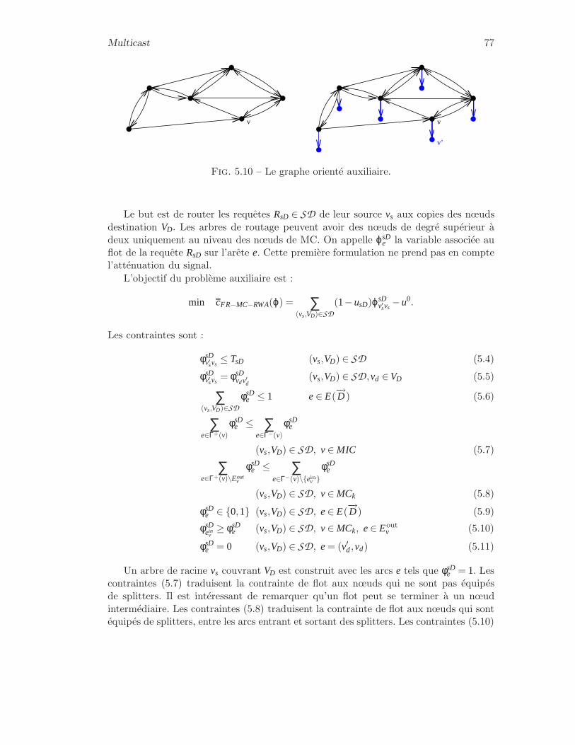
Multicast 77
v’
v
v’
v
Fig. 5.10 – Le graphe orienté auxiliaire.
Le but est de router les requêtes RsD ∈ SD de leur source vs aux copies des nœudsdestination VD. Les arbres de routage peuvent avoir des nœuds de degré supérieur àdeux uniquement au niveau des nœuds de MC. On appelle ϕsD
e la variable associée auflot de la requête RsD sur l’arête e. Cette première formulation ne prend pas en comptel’atténuation du signal.
L’objectif du problème auxiliaire est :
min cFR−MC−RWA(ϕ) = ∑(vs,VD)∈SD
(1−usD)ϕsDv′svs
−u0.
Les contraintes sont :
φsDv′svs
≤ TsD (vs,VD) ∈ SD (5.4)
φsDv′svs
= φsDvdv′d
(vs,VD) ∈ SD,vd ∈VD (5.5)
∑(vs,VD)∈SD
φsDe ≤ 1 e∈ E(
−→D ) (5.6)
∑e∈Γ+(v)
φsDe ≤ ∑
e∈Γ−(v)
φsDe
(vs,VD) ∈ SD, v∈ MIC (5.7)
∑e∈Γ+(v)\Eout
v
φsDe ≤ ∑
e∈Γ−(v)\einv
φsDe
(vs,VD) ∈ SD, v∈ MCk (5.8)
φsDe ∈ 0,1 (vs,VD) ∈ SD, e∈ E(
−→D ) (5.9)
φsDein
v≥ φsD
e (vs,VD) ∈ SD, v∈ MCk, e∈ Eout
v (5.10)
φsDe = 0 (vs,VD) ∈ SD, e= (v′d,vd) (5.11)
Un arbre de racine vs couvrant VD est construit avec les arcs e tels que φsDe = 1. Les
contraintes (5.7) traduisent la contrainte de flot aux nœuds qui ne sont pas équipésde splitters. Il est intéressant de remarquer qu’un flot peut se terminer à un nœudintermédiaire. Les contraintes (5.8) traduisent la contrainte de flot aux nœuds qui sontéquipés de splitters, entre les arcs entrant et sortant des splitters. Les contraintes (5.10)

78 Réseaux d’accès et de cœur
traduisent le fait qu’un signal arrivant sur la fibre d’entrée d’un splitter est transmiseà ses fibres de sortie. De cette manière, un ensemble d’arbres arcs-disjoints tel que lesnœuds de degré k+ 1 sont situés aux nœuds de ∪ℓ≥kMCℓ est défini. Cela correspondbien à une configuration.
Atténuation du signal. La formulation suivante permet de prendre en compte l’at-ténuation du signal optique. À chaque arc est associé un coût ae correspondant à l’at-ténuation d’un signal utilisant cet arc. L’atténuation est exprimée en décibels. Il estégalement possible d’inclure à ce coût l’atténuation induite par un splitter puisque leurposition est fixe. Enfin, si des amplificateurs sont utilisés afin de régénérer le signal,leur effet peut aussi être incorporé à ce coût. L’atténuation du signal est une contrainteimportante dans le routage car un signal trop dégradé n’est pas exploitable par lesdestinations. La limite habituellement utilisée est une atténuation de 20 dB. Un nouvelensemble de variables similaires aux variables φsD
e est introduit pour prendre en comptel’atténuation : pour tout e∈ E, tout (vs,VD) ∈ SD et tout d ∈VD, la variable ϕsD,d
e estintroduite. Elle compte l’atténuation du signal allant de s à d ∈VD.
∑d∈D
ϕsD,de ≥ ϕsD
e (vs,VD) ∈ SD,e∈ E (5.12)
∑e
ϕsD,de ae ≤ 20 (vs,VD) ∈ SD,vd ∈VD (5.13)
ϕsD,de ≤ ϕsD
e (vs,VD) ∈ SD,e∈ E(−→D ) (5.14)
ϕsD,dv′svs
= ϕsD,dvdv′d
(vs,VD) ∈ SD,vd ∈VD (5.15)
ϕsD,de ∈ 0,1 (vs,VD) ∈ SD, e∈ E(
−→D ) (5.16)
∑e∈Γ+(v)
ϕsD,de = ∑
e∈Γ−(v)
ϕsD,de (vs,VD) ∈ SD, vd ∈VD,e∈ E(
−→D ) (5.17)
Ces équations sont adaptables aux autres formulations que je propose. Les variablesϕsD,d
e définissent un chemin de vs à vd. Les équations 5.15 assurent qu’elles utilisent unchemin réservé pour la requête. L’équation 5.14 s’assure que sur ce chemin, l’atténuationglobale ne dépasse pas 20 dB ; si c’est le cas les variables ϕsD,d
e sont forcées d’être à 0,ce qui, par les équations 5.12, empêche la requête d’être satisfaite.
5.2.4.3 Problème FR-MC-RWA : formulation par arbres de routage
Problème maître. Dans cette formulation, le problème maître est résolu sur unsous-ensemble de T (c.f. Section 5.2.3) et sélectionne un ensemble d’arbres de routageet de longueurs d’onde afin de satisfaire un maximum de requêtes. La contrainte quedeux arbres de routage ayant la même longueur d’onde ne partagent pas d’arc estvérifiée dans le problème maître. Le problème auxiliaire inclut les autres contraintesde FR-MC-RWA qui indiquent que les nœuds de grand degré des arbres de routagedoivent correspondre avec les nœuds de MC.

Multicast 79
Un arbre de routage t est représenté par un ensemble de variables δe,t qui valent 1si l’arc e est utilisé par l’arbre de routage et 0 sinon. Chaque variable wλ
t du problèmemaître est associée à un arbre de routage t et à une longueur d’onde λ. wλ
t vaut 1 sil’arbre de routage t est utilisé sur la longueur d’onde λ, 0 sinon.
Le problème maître est :
max zmax MC−RWA−lt(w) = ∑λ∈Λ
∑t∈T
wλt
sujet à :
∑t∈T
δe,twλt ≤ 1 λ ∈ Λ, e∈ E (u0
λe) (5.18)
∑λ∈Λ
∑t∈TsD
wλt ≤ TsD (vs,VD) ∈ SD (u1
sD) (5.19)
wλt ∈ N t ∈ T , λ ∈ Λ. (5.20)
(u0λe) et (u1
sD) sont les variables duales associées aux contraintes (5.18-e) et (5.19-(vs,VD)).
Problème auxiliaire. Il y a un problème auxiliaire différent pour chaque longueurd’onde. Étant donnée une longueur d’onde λ, on considère le graphe orienté associéau réseau. À chaque arc e on associe comme coût la variable duale (u0
λe). Le problèmeauxiliaire est un problème de flot sur ce graphe orienté. Deux familles de variables sontutilisées : ϕλ
e est la variable de flot associée à l’arc e et ϕλsD indique le nombre d’arbres
de routage de racine vs couvrant VD.Étant donnée une longueur d’onde λ, l’objectif du problème auxiliaire est :
max 1−∑e∈t
u0λeϕλ
e −∑sD
u1sDϕλ
sD
sous les contraintes :∑sD
ϕλsD = 1 e∈ E (5.21)
∑vs:(vs,VD)∈SD ,vi∈VD
ϕλsD + ∑
e∈Γ+(vi)
ϕλe = ∑
e∈Γ−(vi)
ϕλe + ∑
VD:(vi ,VD)∈SDϕλ
sD, vi ∈ MIC (5.22)
∑vs:(vs,VD)∈SD ,vi∈VD
ϕλsD+ ∑
e∈Γ+(vi)\Eoutvi
ϕλe = ∑
e∈Γ−(vi)\einvi
ϕλe + ∑
VD:(vi ,VD)∈SDϕλ
sD, vi ∈MCi (5.23)
φsDein
v≥ φsD
e , (vs,VD) ∈ SD, v∈ MCk, e∈ Eoutv (5.24)
ϕλsD ∈ 0,1 (vs,VD) ∈ SD (5.25)
ϕλe ∈ 0,1 e∈ D (5.26)
80 Réseaux d’accès et de cœur
Le problème auxiliaire consiste à trouver un arbre de coût minimum, il s’agit donc detrouver un arbre de Steiner pour chaque requête, or ce problème est NP-dur. Cependantsi les multicasts sont suffisamment petits, on peut utiliser un algorithme exact (decomplexité en 2kn3 où k est le nombre de destinataires du multicast), mais il ne fautpas oublier les contraintes imposées par les splitters.
5.2.5 Problème PR-MC-RWA
Dans les réseaux d’accès les signaux sont émis avec moins de puissance que dans lecas des réseaux de cœur, le coût des lasers utilisés est alors beaucoup plus faible ce quipermet d’en utiliser plusieurs par multicast. Ainsi, dans un réseau d’accès, un multicastpeut être émis en plusieurs fois. Cela signifie qu’une requête peut être satisfaite par uneunion d’arbres. Ce problème introduit dans [HCT01], a encore été peu étudié.
5.2.5.1 Problème PR-MC-RWA : formulation avec configuration de rou-tage
Je présente une formulation pour le problème PR-MC-RWA basée sur le conceptde configuration de routage. Le principe est similaire à celui de la Section 5.2.4.2.Une configuration de routage pour PR-MC-RWA est associée à un ensembled’arbres qui peuvent tous être routés sur une même longueur d’onde. Chaque arbresert une requête, il peut éventuellement la servir partiellement. Je rappelle que dansPR-MC-RWA, une source peut envoyer plusieurs fois le même message et une requêtene doit pas forcément être satisfaite complètement. Soit CPR−MC−RWA l’ensemble detoutes les configurations de routage pour PR-MC-RWA. Une configuration de routageest représentée par un vecteur C. Chaque variable wC du problème maître est associéeà l’une d’entre elles. La valeur de wC indique le nombre de fois où la configuration Cest utilisée dans la solution. Étant donné un vecteur C associé à une configuration deroutage, à chaque requête (vs,VD) et à chaque sous-ensemble de nœuds de destinationV ′
D ⊂VD est associé une ligne de C : C(sD′), elle indique le nombre d’arbres de routagede racine vs et couvrant V ′
D dans cette configuration.Cette formulation permet de partager une requête en plusieurs requêtes pour la
router. En particulier, on peut router une requête sur plusieurs longueurs d’onde.
Problème maître. L’objectif du problème maître est :
max zPR−MC−RWA−irc(w) = ∑C∈C
∑(vs,VD)∈SD ,V ′
D⊂VD
|V ′D|zsD
sD′ (5.27)
sujet à :
∑C∈C
wC ≤W (u0) (5.28)
wC ∈ N C∈ C (u1sD). (5.29)
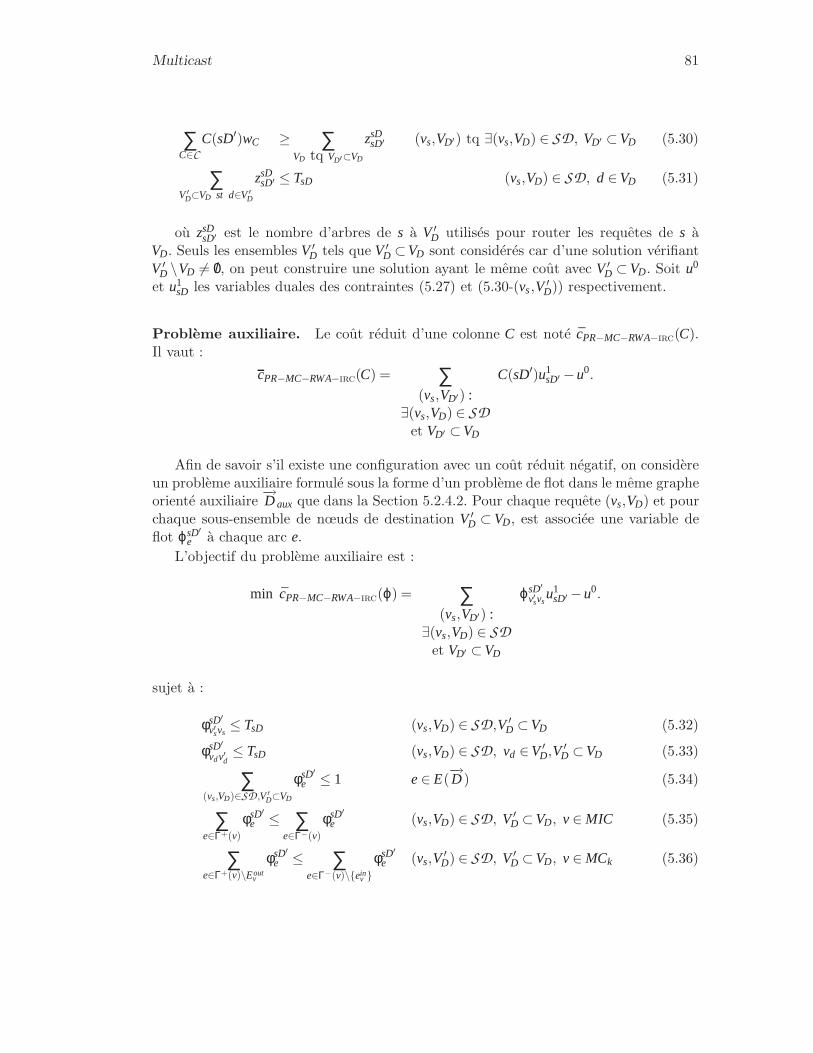
Multicast 81
∑C∈C
C(sD′)wC ≥ ∑VD tq VD′⊂VD
zsDsD′ (vs,VD′) tq ∃(vs,VD) ∈ SD, VD′ ⊂VD (5.30)
∑V ′
D⊂VD st d∈V ′D
zsDsD′ ≤ TsD (vs,VD) ∈ SD, d ∈VD (5.31)
où zsDsD′ est le nombre d’arbres de s à V ′
D utilisés pour router les requêtes de s àVD. Seuls les ensembles V ′
D tels que V ′D ⊂VD sont considérés car d’une solution vérifiant
V ′D \VD 6= /0, on peut construire une solution ayant le même coût avec V ′
D ⊂VD. Soit u0
et u1sD les variables duales des contraintes (5.27) et (5.30-(vs,V ′
D)) respectivement.
Problème auxiliaire. Le coût réduit d’une colonne C est noté cPR−MC−RWA−irc(C).Il vaut :
cPR−MC−RWA−irc(C) = ∑(vs,VD′) :
∃(vs,VD) ∈ SDet VD′ ⊂VD
C(sD′)u1sD′ −u0.
Afin de savoir s’il existe une configuration avec un coût réduit négatif, on considèreun problème auxiliaire formulé sous la forme d’un problème de flot dans le même grapheorienté auxiliaire
−→D aux que dans la Section 5.2.4.2. Pour chaque requête (vs,VD) et pour
chaque sous-ensemble de nœuds de destination V ′D ⊂ VD, est associée une variable de
flot ϕsD′e à chaque arc e.
L’objectif du problème auxiliaire est :
min cPR−MC−RWA−irc(ϕ) = ∑(vs,VD′) :
∃(vs,VD) ∈ SDet VD′ ⊂VD
ϕsD′v′svs
u1sD′ −u0.
sujet à :
φsD′v′svs
≤ TsD (vs,VD) ∈ SD,V ′D ⊂VD (5.32)
φsD′vdv′d
≤ TsD (vs,VD) ∈ SD, vd ∈V ′D,V ′
D ⊂VD (5.33)
∑(vs,VD)∈SD ,V ′
D⊂VD
φsD′e ≤ 1 e∈ E(
−→D ) (5.34)
∑e∈Γ+(v)
φsD′e ≤ ∑
e∈Γ−(v)
φsD′e (vs,VD) ∈ SD, V ′
D ⊂VD, v∈ MIC (5.35)
∑e∈Γ+(v)\Eout
v
φsD′e ≤ ∑
e∈Γ−(v)\einv
φsD′e (vs,V
′D) ∈ SD, V ′
D ⊂VD, v∈ MCk (5.36)
82 Réseaux d’accès et de cœur
φsD′ein
v≥ φsD′
e (vs,VD) ∈ SD,V ′D ⊂VD,v∈ MCk, e∈ Eout
v (5.37)
φsD′e = 0 (vs,VD) ∈ SD,V ′
D ⊂VD,e= (v′d,vd) (5.38)
φsDv′svs
= φsDvdv′d
(vs,VD) ∈ SD, V ′D ⊂VD (5.39)
φsD′e ∈ 0,1 (vs,VD) ∈ SD, V ′
D ⊂VD e∈ E (5.40)
Les arcs e avec φsD′e = 1 forment un arbre de routage de racine vs couvrant V ′
D. Lescontraintes (5.35) traduisent la contrainte de flot aux nœuds qui ne sont pas équipésde splitters. Les contraintes (5.36) traduisent la contrainte de flot aux nœuds qui sontéquipés de splitters. Les contraintes (5.37) traduisent le fait qu’un signal arrivant surla fibre d’entrée d’un splitter est transmise à ses fibres de sortie. De cette manière, ondéfinit un ensemble d’arbres arcs-disjoints tel que les nœuds des arbres de degré k+1sont situés aux nœuds du réseau appartenant à ∪ℓ≥kMC_ℓ. Cela correspond bien à uneconfiguration.
Remarque 5.21 J’ai décrit deux formulations mathématiques pour résoudre le pro-blème MC-RWA. La dernière formulation a pour but de résoudre ce problème dans lesréseaux d’accès. Cependant cette formulation ne prend pas en compte la faible densitédes réseaux d’accès, or cette particularité peut aider dans le choix des arbres de routage.Dans la section suivante, notre but est de proposer une autre manière de résoudre leproblème MC-RWA en prenant en compte la structure des réseaux d’accès.
5.2.6 Réseaux d’accès
Dans la continuité du travail précédent, je regarde le problème du routage de mul-ticasts dans les réseaux d’accès. Le but de ces réseaux est de relier individuellementles clients aux réseaux de cœur. Le besoin de bande passante des réseaux d’accès arapidement augmenté ces dernières années.
De nos jours, la majorité des réseaux déployés sont de type DSL (digital suscriber,ligne d’abonné numérique), ou CATV (Cable Television, télévision par câble). Ces deuxtechnologies ont été développées pour transporter la voix et les signaux télévisuelsrespectivement et ne sont pas adaptés aux besoins actuels.
5.2.6.1 Réseaux Passifs Optiques
Les réseaux passifs optiques (PON, passive optical networks) ont pour butd’offrir une plus grande bande passante dans les réseaux d’accès. Leur rôle est de relierun terminal optique (OLT, optical line terminal) aux clients (ONU, opticalnetwork units) et pour cela, des splitters sont utilisés. Le réseau entre les ONUs etl’OLT est passif : il ne nécessite pas d’énergie. Ces dernières années, diverses versionsdes PONs sont apparues. L’ATM Passive Optical Network (APON) est le premierstandard pour les réseaux passifs optiques suivi par l’Ethernet PON (EPON) qui estun standard IEEE/EFM permettant d’utiliser le protocole Ethernet. Le Broadband
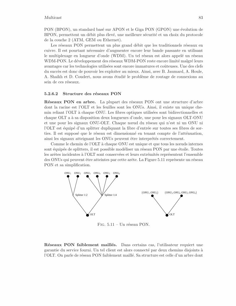
Multicast 83
PON (BPON), un standard basé sur APON et le Giga PON (GPON) une évolution deBPON, permettent un débit plus élevé, une meilleure sécurité et un choix du protocolede la couche 2 (ATM, GEM ou Ethernet).
Les réseaux PON permettent un plus grand débit que les traditionnels réseaux encuivre. Il est pourtant nécessaire d’augmenter encore leur bande passante en utilisantle multiplexage en longueur d’onde (WDM). Un tel réseau est alors appelé un réseauWDM-PON. Le développement des réseaux WDM-PON reste encore limité malgré leursavantages car les technologies utilisées sont encore immatures et coûteuses. Une des clefsdu succès est donc de pouvoir les exploiter au mieux. Ainsi, avec B. Jaumard, A. Houle,A. Shaikh et D. Coudert, nous avons étudié le problème de routage de connexions ausein de ces réseaux.
5.2.6.2 Structure des réseaux PON
Réseaux PON en arbre. La plupart des réseaux PON ont une structure d’arbredont la racine est l’OLT et les feuilles sont les ONUs. Ainsi, il existe un unique che-min reliant l’OLT à chaque ONU. Les fibres optiques utilisées sont bidirectionnelles etchaque OLT a à sa disposition deux longueurs d’onde, une pour les signaux OLT-ONUet une pour les signaux ONU-OLT. Chaque nœud du réseau qui n’est ni un ONU nil’OLT est équipé d’un splitter dupliquant la fibre d’entrée sur toutes ses fibres de sor-ties. Il est supposé que le réseau est dimensionné en tenant compte de l’atténuation,ainsi les signaux atteignant les ONUs peuvent être interprétés correctement.
Comme le chemin de l’OLT à chaque ONU est unique et que tous les nœuds internessont équipés de splitters, il est possible modéliser un réseau PON par une étoile. Toutesles arêtes incidentes à l’OLT sont conservées et leurs extrémités représentent l’ensembledes ONUs qui peuvent être atteintes par cette arête. La Figure 5.11 représente un réseauPON et sa simplification.
Splitter 1:2 Splitter 1:4
OLT
ONU1 ONU2 ONU3 ONU4 ONU5 ONU6
OLT
ONU3,ONU4,ONU5,ONU6ONU1,ONU2
Fig. 5.11 – Un réseau PON.
Réseaux PON faiblement maillés. Dans certains cas, l’utilisateur requiert unegarantie du service fourni. Un tel client est alors connecté par deux chemins disjoints àl’OLT. On parle de réseau PON faiblement maillé. Sa structure est celle d’un arbre dont

84 Réseaux d’accès et de cœur
certaines feuilles sont fusionnées. L’ONU placé à un tel nœud peut alors recevoir sesmessages par deux chemins différents. Cependant, un message destiné à un autre ONUne peut pas être routé par ce nœud car l’équipement installé ne le permet pas. Commepour les réseaux PON en forme d’arbre, les réseaux PON faiblement maillés peuventêtre représentés par une étoile. La différence est qu’un ONU peut être présent dans lesensembles de plusieurs feuilles. La Figure 5.12 illustre un réseau PON faiblement maillédans lequel l’ONU2 est relié à l’OLT par deux chemins disjoints, et sa modélisation. LaFigure 5.13, représente un routage autorisé et un routage interdit dans un réseau PONfaiblement maillé.
Splitter 1:2 Splitter 1:4
OLT
ONU1 ONU5ONU4ONU3ONU2
(a) Un réseau PON faible-ment maillé.
OLT
ONU1,ONU2 ONU2,ONU3,ONU4,ONU5
(b) Modélisation d’unréseau PON faible-ment maillé.
Fig. 5.12 – Un réseau PON faiblement maillé et sa modélisation.
Splitter 1:2 Splitter 1:4
OLT
ONU1 ONU5ONU4ONU3ONU2
(a) Un routage valide.
Splitter 1:2 Splitter 1:4
OLT
ONU1 ONU5ONU4ONU3ONU2
(b) Un routage non valide.
Fig. 5.13 – La validité des routages dans un réseau PON faiblement maillé.

Conclusion et Perspectives 85
5.2.6.3 Modèles
Dans l’Annexe C.2 sont décrits quatre modèles différents pour le problème MC-RWAdans les réseaux PONs.
Le premier objectif considéré est de maximiser le nombre de requêtes servies dansles réseaux PON ayant une structure d’arbre puis dans les réseaux PON faiblementmaillés. On modélise à la fois le cas où le multiplexage temporel n’est pas utilisé et lecas où il est utilisé.
Ensuite on étudie les mêmes problèmes avec pour objectif de maximiser le nombred’ONUs (clients) servis. Comme dit dans la section précédente, cet objectif est le pluspertinent dans les réseaux d’accès. L’implémentation de ces modèles est en cours, ce quiva permettre de comparer les différents modèles entre eux, et en particulier d’estimerle gain obtenu en maximisant le nombre d’ONUs servis au lieu du nombre de requêtessatisfaites.
5.3 Conclusion et Perspectives
Dans ce chapitre, j’ai commencé par présenter l’intérêt de l’usage du multicastdans les réseaux. Dans la première section, j’ai décrit les technologies optiques utiliséesaujourd’hui et qui concernent les problème que j’étudie. Dans la Section 5.2.1, j’aidécrit un problème de coloration de graphes orientés relié au routage de multicasts etqui permet d’évaluer le gain apporté par des splitters en longueurs d’onde. Ensuitej’ai présenté des formulations mathématiques permettant de résoudre le problème MC-RWA dans les réseaux de cœurs et les réseaux d’accès. Dans la dernière section, j’aiprésenté les travaux en cours sur des formulations du problème MC-RWA dans lesréseaux PON.
Il reste à finir l’implémentation des formulations mathématiques afin de pouvoircomparer les solutions que l’on propose à des solutions déjà existantes. Il est égale-ment intéressant de considérer le problème de fiabilité des connexions établies. Dans leprochain chapitre, on s’intéresse à ce problème dans le cas des requêtes unicasts.

86 Réseaux d’accès et de cœur
Chapitre 6
Fiabilité et tolérance aux pannes
Dans ce chapitre j’étudie des problèmes reliés à la fiabilité des communicationsdans un réseau. Je commence par présenter le problème des pannes multiples duesaux groupes de risques et une formulation mathématique permettant de prendreen compte ces risques lors du routage. Dans une seconde section, je présente desmodèles pour un mode de protection des connexions par segments.
Lors de l’exploitation d’un réseau, la minimisation des capacités utilisées n’est pasle seul critère à prendre en compte. En effet, il est nécessaire de s’assurer que les clientssont satisfaits du service rendu. Par conséquent, il faut garantir une continuité du serviceet ce, même si des composants du réseau tombent en panne. Ce chapitre est dédié à cetteproblématique. Il est composé de deux sections, dans la première je présente les pro-blèmes induits par un réseau multicouche et je propose un moyen pour en tenir compte.Ces travaux font suite à la thèse de M-E. Voge, [Vog06b] et à [CPRV06, CDP+07]. Dansla deuxième section, je présente une formulation mathématique permettant de calculerdes protections pour un ensemble de chemins préétablis.
6.1 Réseaux colorés
Les pannes multiples sont intrinsèquement liées aux réseaux multicouches. Les ré-seaux colorés ont été introduits pour modéliser de telles pannes. Dans cette section, jeprésente une formulation mathématique du problème de routage permettant de prendreen compte les pannes multiples. Ces travaux ont donné lieu à un article qui a été pré-senté lors la conférence ICC 2008 et qui peut être trouvé dans l’Annexe D.1.
87
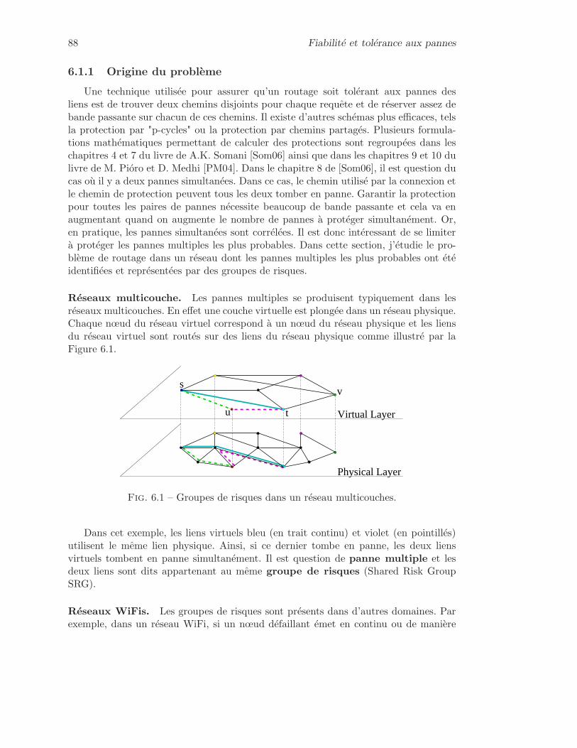
88 Fiabilité et tolérance aux pannes
6.1.1 Origine du problème
Une technique utilisée pour assurer qu’un routage soit tolérant aux pannes desliens est de trouver deux chemins disjoints pour chaque requête et de réserver assez debande passante sur chacun de ces chemins. Il existe d’autres schémas plus efficaces, telsla protection par "p-cycles" ou la protection par chemins partagés. Plusieurs formula-tions mathématiques permettant de calculer des protections sont regroupées dans leschapitres 4 et 7 du livre de A.K. Somani [Som06] ainsi que dans les chapitres 9 et 10 dulivre de M. Pióro et D. Medhi [PM04]. Dans le chapitre 8 de [Som06], il est question ducas où il y a deux pannes simultanées. Dans ce cas, le chemin utilisé par la connexion etle chemin de protection peuvent tous les deux tomber en panne. Garantir la protectionpour toutes les paires de pannes nécessite beaucoup de bande passante et cela va enaugmentant quand on augmente le nombre de pannes à protéger simultanément. Or,en pratique, les pannes simultanées sont corrélées. Il est donc intéressant de se limiterà protéger les pannes multiples les plus probables. Dans cette section, j’étudie le pro-blème de routage dans un réseau dont les pannes multiples les plus probables ont étéidentifiées et représentées par des groupes de risques.
Réseaux multicouche. Les pannes multiples se produisent typiquement dans lesréseaux multicouches. En effet une couche virtuelle est plongée dans un réseau physique.Chaque nœud du réseau virtuel correspond à un nœud du réseau physique et les liensdu réseau virtuel sont routés sur des liens du réseau physique comme illustré par laFigure 6.1.
s
u
v
t
Physical Layer
Virtual Layer
Fig. 6.1 – Groupes de risques dans un réseau multicouches.
Dans cet exemple, les liens virtuels bleu (en trait continu) et violet (en pointillés)utilisent le même lien physique. Ainsi, si ce dernier tombe en panne, les deux liensvirtuels tombent en panne simultanément. Il est question de panne multiple et lesdeux liens sont dits appartenant au même groupe de risques (Shared Risk GroupSRG).
Réseaux WiFis. Les groupes de risques sont présents dans d’autres domaines. Parexemple, dans un réseau WiFi, si un nœud défaillant émet en continu ou de manière

Réseaux colorés 89
aléatoire, à cause des interférences, ses autres voisins sont incapables de recevoir unmessage, comme indiqué sur la Figure 6.2.
B
A
C
D
Fig. 6.2 – Groupes de risques dans un réseau radio.
Réseaux routiers. Les groupes de risques sont également présents dans les réseauxroutiers : si deux routes A et B se croisent et que la route A est bloquée, dès qu’unevoiture de la route B veut tourner sur la route A, la route B se retrouve bloquée, c.f.Figure 6.3.
B
A
Fig. 6.3 – Groupes de risques dans un réseau routier.
Plan. Dans cette section, mon objectif est de proposer une formulation mathématiquepermettant de trouver un routage des requêtes qui prend en compte les groupes derisques. Une connexion qui utilise des liens qui font partie de peu de groupes de risquesdifférents a en effet moins de chance d’être interrompue. Par la suite, il sera égalementplus aisé de rajouter des chemins de protection n’utilisant pas les même groupes derisques.
90 Fiabilité et tolérance aux pannes
6.1.2 Notations
Tout au long de cette section, je considère un réseau composé de deux couches : unecouche physique et une couche virtuelle. Cela permet d’illustrer l’origine des groupesde risques, mais les résultats présentés sont valables pour tout réseau dont les groupesde risques sont connus.
La couche physique est représentée par un graphe orienté DPN = (VPN,EPN), où VPN
est l’ensemble des sommets et EPN = e1, . . .em l’ensemble des liens (c.à.d. les fibresunidirectionnelles). De même, le réseau virtuel est représenté par un graphe orientéDVN = (VVN ,EVN). Chaque arc e∈ EVN a un coût pe par unité de flot et une capacité ue.
À chaque arc ei du réseau physique DPN correspond un groupe de risques dans leréseau virtuel ci , désigné par une couleur. Plus précisément, une couleur ci correspond àun sous-ensemble d’arcs (du réseau virtuel) routés sur l’arc ei (dans le réseau physique).Autrement dit, c’est l’ensemble des liens virtuels coupés en cas de panne de l’arc ei .C = c1, . . . ,cm est l’ensemble des couleurs (c.à.d. des SRGs) du réseau. Un même arcpeut appartenir à plusieurs groupes de risques différents. Pour pallier à cela chaque arcest remplacé par une chaîne d’arcs, chacun appartenant à un unique groupe de risques,comme proposé dans [CDP+07, Vog06a]. Par simplicité, le graphe orienté modifié esttoujours appelé DVN. Un graphe orienté dans lequel tout arc a exactement une couleurest appelé graphe orienté coloré.
T est la matrice des requêtes à router dans DVN . A chaque requête tsd ∈ T sontassociées sa source vs, sa destination vd et sa taille Tsd. Je note |T|= ∑tsd∈T Tsd. La taillede chaque requête est supposée entière, et une requête peut être partagée en requêtesunitaires qui peuvent être routées indépendamment. Pour chaque requête tsd ∈ T, P sd
est l’ensemble de tous les chemins de vs à vd dans DVN et P = ∪tsd∈TPsd.
Je rappelle que Γ−(v) et Γ+(v) représentent l’ensemble des arcs entrant et sortantde v.
Enfin, étant donné un graphe (respectivement graphe orienté) coloré, le span d’unecouleur est le nombre de composantes connexes induites par cette couleur. Si dansun graphe (respectivement graphe orienté) coloré toutes les couleurs ont "span 1", celasignifie que les groupes de risques sont locaux et dans ce cas, certains problèmes commele MCP (problème de trouver un chemin avec le moins de couleurs possible pour unerequête) devient polynomial.
6.1.3 Problème et complexité
Problème 6.1 (Flot minimum en nombre de couleurs moyen (Minimun Ave-rage Color Flow) MACF)
Entrées : Un graphe orienté coloré représentant un réseau (virtuel).Des coûts et des capacités sur les liens du réseau.Un ensemble de requêtes entières.
Sortie : Un routage (chemin et longueur d’onde) des requêtes.Objectif : Minimiser α∑coût des arcs+(1−α)∑#srg moyen.
Il se trouve que ce problème est dur à résoudre et ce même dans des cas simples.

Réseaux colorés 91
Complexité, coût des liens nul : ∀e∈ E, pe = 0. Avec un coût nul sur les liens,le problème de router une requête est connu comme le problème Minimum Color Path(MCP) qui a été montré NP-dur dans [YVJ05]. Le théorème suivant donne égalementun résultat d’inaproximabilité. Il a été prouvé dans le cas des graphes non orientés maissa généralisation aux graphes orientés est immédiate.
Théorème 6.2 ([CDP+07]) Le problème Minimum Color Path est NP-dur et dur à
approximer à un facteur 2log1−δ |C |12 près, avec δ = (log log|C | 1
2 )−ε et ε < 12.
Complexité, toutes les couleurs ont span 1. Nous avons montré dans [CHPV08]le théorème suivant qui s’applique aux réseaux dont les arcs n’ont pas un coût nul :
Théorème 6.3 Étant donné un graphe orienté symétrique coloré où toutes les cou-leurs ont span 1, le problème MCP avec coût sur les arcs (MCP with edge cost, noté
MCPwEC) est NP-dur et dur à approximer à un facteur 2log1−δ |C |12 près, avec δ =
(log log|C | 12 )−ε et ε < 1
2.
6.1.4 Formulations
6.1.4.1 Formulation sommet-arc
Pour résoudre le problème MACF, dans [CHPV08], avec D. Coudert, F. Peix et M-E. Voge, nous avons proposé deux formulations. Une première formulation sommet-arcet une seconde formulation arc-chemin sous forme de génération de colonnes.
Pour la formulation sommet-arc, nous utilisons une variable de flot binaire φsde pour
tout lien e∈ EVN et toute requête tsd ∈ T. φsde vaut 1 si le lien virtuel e est utilisé pour
router la requête unitaire tsd, 0 sinon.Des variables binaires sont utilisées pour les couleurs : χc
sd, pour tout tsd ∈ T etc∈ C . χc
sd vaut 1 si la requête unitaire tsd est routée sur un arc appartenant au groupede risque représenté par la couleur c.
min1|T| ∑tsd
(
α ∑c∈C
χcsd+(1−α) ∑
e∈E
peφsde
)
∑e∈Γ+(v)
zke− ∑
e∈Γ−(v)
zke =
1 if v = sk
-1 si v = tk0 sinon
∀k∈ K (6.1)
∑k∈K
zke ≤ ue ∀e∈ LVN (6.2)
zke ≤ χc(e)
k ∀k,∀e∈ LVN (6.3)
Les contraintes (6.1) et (6.2) sont les contraintes classiques de conservation du flotet de capacité des liens du réseau. La contrainte (6.3) assure que chaque fois qu’unerequête utilise un lien e, la variable de couleur correspondant à la couleur de ce lienvaut 1 ce qui indique que la requête utilise cette couleur. Il y a |T|(|EVN |+ |C |) variableset |T|(|VVN |+ |EVN|)+ |EVN| contraintes.
92 Fiabilité et tolérance aux pannes
6.1.4.2 Formulation arc-chemin
φsdP est une variable binaire qui vaut 1 si la requête tsd∈ T est routée sur un chemin
P∈ P , et 0 sinon. Le nombre de chemins permettant de router une requête peut êtreexponentiel, il se peut qu’il y ait un nombre exponentiel de variables de ce type. Demême que dans la formulation sommet-arc, des variables binaires χc
sd indiquent si unchemin qui est utilisé par une requête utilise un arc de couleur c ou pas.
Objectif :
min1|T| ∑tsd
(
α ∑c∈C
χc(e)sd +(1−α) ∑
e∈EVN
∑P∈P sd|e∈P
peφsdP
)
Contraintes :
∑P∈P sd
φsdP = 1 ∀tsd∈ T (σsd) (6.4)
∑tsd
∑P∈P sd|e∈P
φsdP ≤ ue ∀e∈ EVN (ωe) (6.5)
∑P∈P sd|e∈P
φsdP ≤ χc(e)
sd ∀tsd∈ T,∀e∈ EVN (πsde ) (6.6)
Les contraintes (6.4) assurent que toutes les requêtes sont bien satisfaites ; σsd sontles variables duales associées. La contrainte de capacité (6.5) sur chaque lien impliquequ’il ne peut pas y avoir plus de chemins utilisant un même lien e que la capacité de celien le permet ; ωe sont les variables duales associées. De même que dans la formulationsommet-arc, les contraintes (6.6) indiquent les couleurs utilisées pour servir chaquerequêtes, les variables duales associées sont (πsd
e ).La fonction objectif est la même.Pour résoudre ce programme linéaire, la technique de génération de colonnes est
utilisée. Il y a |T|(|EVN |+1)+ |EVN | contraintes et de manière empirique, au plus 10|T|variables sont générées. Cela est bien plus faible que dans la formulation sommet-arc.
6.1.4.3 La génération de colonnes appliquée à MACF
Problème maître. Le problème maître est une restriction de la formulation arc-chemin sur un sous-ensemble des chemins disponibles, c.à.d. que seule une partie desvariables φsd
P P∈P sd est considérée. Les autres variables n’existent tout simplement pas.
Problème auxiliaire. Étant donnée une requête tsd, le problème auxiliaire est unproblème de plus court chemin sur le graphe DVN avec comme coût sur les liens (1−α)
|T| pe+
ωe+ πsde . Le coût réduit d’un chemin P∈ P sd est :
σsd− ∑e∈P
(
(1−α)
|T| pe+ ω+ πsde
)
Un chemin ayant un coût positif permet d’améliorer la solution du problème maître.

Réseaux colorés 93
Afin de garantir une solution optimale, nous devons résoudre le problème auxiliairepour chaque requête tsd ∈ T. Étant donné que le coût d’une couleur (χc(e)
sd ) n’est pas lemême pour chaque requête, le coût assigné aux arcs varie pour chaque requête.
Génération de la solution initiale. Pour générer la solution initiale, un multiflotclassique est résolu, sans tenir compte des couleurs.
Solution entière. Dans la solution obtenue, les variables φsdP et χc
sd sont fraction-naires. Il est nécessaire de faire du branchement (fixer la valeur d’une variable et ré-soudre de nouveau le problème de manière récursive) pour trouver une solution entière.Il est intéressant de noter qu’il n’est pas nécessaire de brancher sur les variables χc
sdcar il est possible de les considérer comme fractionnaires. En effet, puisque toutes lesrequêtes sont unitaires, lorsque les variables de flot sont entières, les contraintes (6.6)forcent les variables χc
sd à être entières.
6.1.5 Résultats expérimentaux
6.1.5.1 Génération des instances
Pour comparer les deux formulations proposées, nous avons généré des exemplesà partir d’un graphe orienté représentant un réseau physique et d’un graphe orientéreprésentant un réseau virtuel.
Les réseaux physiques ont été conçus à partir de graphes, que nous avons transformésen graphes orientés en remplaçant chaque arête par un circuit de longueur deux. Àchaque arc des graphes orientés obtenus est associée une couleur différente (chaquecouleur représentant un groupe de risques). Si les réseaux physiques possèdent déjà desgroupes de risques, ils peuvent tout aussi bien être utilisés.
Ensuite, un réseau virtuel est généré en plusieurs étapes :
1. Un graphe non orienté sur l’ensemble des sommets du réseau physique est généréen utilisant un générateur de graphes aléatoires implémenté dans mascopt. Legraphe aléatoire requis, a un diamètre d’au plus trois, une coupe minimale d’aumoins deux et environ trois fois plus d’arêtes que de sommets.
2. Chaque arête est remplacée par un circuit de longueur deux.
3. Des requêtes unitaires sont générées de manière aléatoire.
4. Un double multiflot est calculé : les requêtes sont routées sur le graphe orientégénéré précédemment qui lui-même est routé simultanément sur le graphe orientéreprésentant le réseau physique.
5. À chaque arc du graphe orienté généré correspond un ensemble de liens virtuelsparallèles : chaque arc du graphe orienté généré est routé sur un ensemble dechemins, chacun donnant un lien virtuel différent. À chaque lien virtuel sontassociées les couleurs des ressources physiques qu’il utilise. Ceci donne le réseauvirtuel qui est utilisé ainsi que ses groupes de risques.

94 Fiabilité et tolérance aux pannes
6. Le routage des requêtes dans le réseau virtuel donne un poids aux liens virtuels.Chaque liens virtuel vl a un poids poids(vl ) dans le routage ci-dessus. Étant donnéun lien physique pl sur lequel vl est routé, la capacité locale de vl est notée :capacitélocale(vl ), la proportion de capacité de pl qui peut être attribuée à vl si lacapacité de pl est répartie entre les liens virtuels l’utilisant v′l ∈ pl proportionnel-lement à leur poids :
capacitélocale(vl ) =poid(vl )
∑v′l∈plpoid(v′l )
capacité(pl )
La capacité donnée à chaque lien virtuel vl est alors le minimum des capacitéslocales : capacité(vl ) = minpl∋vl (capacitélocale(vl ))
7. Enfin, chaque arc est remplacé par une chaîne d’arcs, chacun des nouveaux arcsappartenant à un unique groupe de risques [CDP+07].
6.1.5.2 Résultats
Les tests ont été réalisés sur un Intel Core 2 2.4 GHz avec 4Mb de L1 cache et 2Gb de mémoire, le programme a été écrit en utilisant la bibliothèque Mascopt. Nousavons utilisé comme réseaux physiques les réseaux NSFnet (14 nœuds et 21 liens) etBrazil (27 nœuds et 70 liens) [NR06]. Le nombre de requêtes était 140 pour NSFnetet 200 pour Brazil. Nous avons réalisé dix tests pour chaque instance du problème,demandant à chaque fois une solution entière à au plus 5 % de la solution optimale(sauf pour α ≥ 0.75, où nous avons demandé 10 %).
Je présente nos résultats sur deux graphiques, un pour Brazil et un pour NSFnet.La hauteur des rectangles représente le temps de calcul. Pour la formulation arc-chemin,le rectangle est partagé en trois : le temps passé à résoudre le problème maître, àrésoudre le problème auxiliaire et à trouver une solution entière.
Fig. 6.4 – Comparaison des temps de calcul pour le réseau Brazil.
Temps de calcul. De manière surprenante le temps de calcul de la formulationsommet-arc est toujours inférieur à celui de la formulation arc-chemin utilisant la gé-nération de colonnes alors que le nombre de variables est bien plus élevé. Cela peut enpartie être expliqué par le fait que pour implémenter la génération de colonnes, nousavons été amenés à utiliser une interface java qui fait appel à cplex puis à un Branch
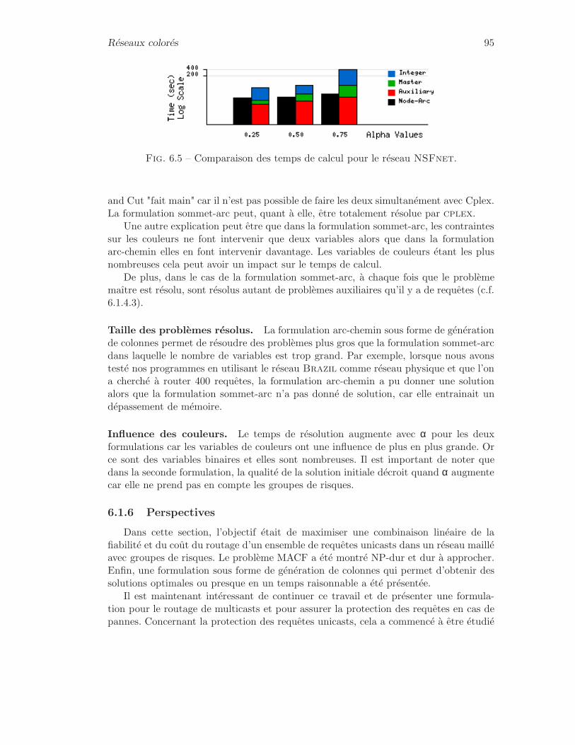
Réseaux colorés 95
Fig. 6.5 – Comparaison des temps de calcul pour le réseau NSFnet.
and Cut "fait main" car il n’est pas possible de faire les deux simultanément avec Cplex.La formulation sommet-arc peut, quant à elle, être totalement résolue par cplex.
Une autre explication peut être que dans la formulation sommet-arc, les contraintessur les couleurs ne font intervenir que deux variables alors que dans la formulationarc-chemin elles en font intervenir davantage. Les variables de couleurs étant les plusnombreuses cela peut avoir un impact sur le temps de calcul.
De plus, dans le cas de la formulation sommet-arc, à chaque fois que le problèmemaître est résolu, sont résolus autant de problèmes auxiliaires qu’il y a de requêtes (c.f.6.1.4.3).
Taille des problèmes résolus. La formulation arc-chemin sous forme de générationde colonnes permet de résoudre des problèmes plus gros que la formulation sommet-arcdans laquelle le nombre de variables est trop grand. Par exemple, lorsque nous avonstesté nos programmes en utilisant le réseau Brazil comme réseau physique et que l’ona cherché à router 400 requêtes, la formulation arc-chemin a pu donner une solutionalors que la formulation sommet-arc n’a pas donné de solution, car elle entrainait undépassement de mémoire.
Influence des couleurs. Le temps de résolution augmente avec α pour les deuxformulations car les variables de couleurs ont une influence de plus en plus grande. Orce sont des variables binaires et elles sont nombreuses. Il est important de noter quedans la seconde formulation, la qualité de la solution initiale décroit quand α augmentecar elle ne prend pas en compte les groupes de risques.
6.1.6 Perspectives
Dans cette section, l’objectif était de maximiser une combinaison linéaire de lafiabilité et du coût du routage d’un ensemble de requêtes unicasts dans un réseau mailléavec groupes de risques. Le problème MACF a été montré NP-dur et dur à approcher.Enfin, une formulation sous forme de génération de colonnes qui permet d’obtenir dessolutions optimales ou presque en un temps raisonnable a été présentée.
Il est maintenant intéressant de continuer ce travail et de présenter une formula-tion pour le routage de multicasts et pour assurer la protection des requêtes en cas depannes. Concernant la protection des requêtes unicasts, cela a commencé à être étudié

96 Fiabilité et tolérance aux pannes
Fig. 6.6 – Évolution du temps de calcul pour le réseau Brésilien.
dans [YVJ05]. Les auteurs y considèrent, comme mode de protection, la protection parchemins en minimisant soit le nombre total de couleurs soit le nombre de couleurs com-munes. Ce travail mérite d’être continué en considérant d’autres types de protection.Dans la section suivante, je fais un premier pas dans cette direction en étudiant unmode de protection alternatif dans des réseaux sans groupes de risques. J’y présenteune formulation mathématique permettant de calculer des protections partagées parsegments, pour un ensemble de chemins préétablis.
6.2 Protection par segments
Je présente un nouveau type de protection partagée spécialement conçu pour pro-téger des routages utilisant la conversion de longueur d’onde dans des réseaux WDM.Son originalité tient du fait qu’elle exploite les équipements déjà installés aux extré-mités des segment des chemins du routage à protéger. Contrairement à la protectionpar lien ou par chemin (dont des formulations mathématiques peuvent être trouvéesdans le livre de A.K. Somani [Som06]), la protection par segment a été peu étudiée,elle permet pourtant de réaliser un compromis intéressant entre la capacité utilisée parla protection et le temps nécessaire pour mettre en place le nouveau routage en casde panne. Je présente deux types de protection par segments différents : la protectionpar segments partagés de base et la protection par segments partagés avec overlaps. Cedernier type de protection est à comparer à un autre, introduit par P-H. Ho et H.T.Mouftah dans [HM02], tant en terme d’architecture que de mécanisme de signalisation.
6.2.1 Contexte
Groupage de trafic. Comme la taille d’une requête peut être plus petite que lacapacité de transfert offerte par une longueur d’onde, une technique, appelée grou-page de trafic, consiste à regrouper plusieurs requêtes sur une même longueur d’onde.Cela peut être réalisé en faisant du multiplexage temporel, comme c’est le cas dans les
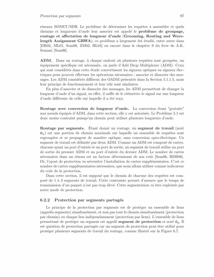
Protection par segments 97
réseaux SONET/SDH. Le problème de déterminer les requêtes à assembler et quelschemins et longueurs d’onde leur associer est appelé le problème de groupage,routage et affectation de longueur d’onde (Grooming, Routing and Wave-length Assignment GRWA), ce problème a largement été étudié, entre autre dans[DR02, ML01, Som06, ZM03, HL04] ou encore dans le chapitre 9 du livre de A.K.Somani [Som06].
ADM. Dans un routage, à chaque endroit où plusieurs requêtes sont groupées, unéquipement spécifique est nécessaire, on parle d’Add Drop Multiplexer (ADM). Ceuxqui sont considérés dans cette étude convertissent les signaux optiques en signaux élec-triques pour pouvoir effectuer les opérations nécessaires : associer et dissocier des mes-sages. Les ADM considérés diffèrent des OADM présentés dans la Section 5.1.1.5, maisleur principe de fonctionnement et leur rôle sont similaires.
En plus d’associer et de dissocier des messages, les ADM permettent de changer lalongueur d’onde d’un signal, en effet, il suffit de le réémettre le signal sur une longueurd’onde différente de celle sur laquelle il a été reçu.
Routage avec conversion de longueur d’onde. La conversion étant "gratuite"aux nœuds équipés d’ADM, dans cette section, elle y est autorisée. Le Problème 5.1 estdonc moins contraint puisqu’un chemin peut utiliser plusieurs longueurs d’onde.
Routage par segments. Étant donné un routage, un segment de travail (notéσw) est une portion de chemin maximale sur laquelle un ensemble de requêtes sontregroupées et se propagent de manière optique, sans conversion opto-électrique. Unsegment de travail est délimité par deux ADM. Comme un ADM est composé de cartes,chacune ayant un port d’entrée et un port de sortie, un segment de travail utilise un portde sortie du premier ADM et un port d’entrée du dernier ADM. Le nombre de cartesnécessaires dans un réseau est un facteur déterminant de son coût [Som06, HDR06].Or, l’ajout de protection va nécessiter l’installation de cartes supplémentaires. C’est cenombre de cartes supplémentaires nécessaires, que nous allons utiliser comme indicateurdu coût de la protection.
Dans cette section, il est supposé que le chemin de chacune des requêtes est com-posé de 1 à 3 segments de travail. Cette contrainte permet d’assurer que le temps detransmission d’un paquet n’est pas trop élevé. Cette segmentation va être exploitée parnotre mode de protection.
6.2.2 Protection par segments partagés
Le principe de la protection par segments est de protéger un ensemble de liens(appelés segments) simultanément, et non pas tout le chemin simultanément (protectionpar chemin) ou chaque lien indépendamment (protection par liens). L’ensemble de lienspermettant de protéger un segment est appelé segment de protection et noté σp. Ilest question de protection partagée car un segment de protection peut être utilisé pourprotéger plusieurs segments de travail du routage, comme illustré sur la Figure 6.7.

98 Fiabilité et tolérance aux pannes
L’idée de protection par segments a déjà été utilisée par Bouffard dans [Bou05]ou Ho et Mouftah dans [HM02]. Cependant dans leurs études, ils ne prennent pas encompte la structure du routage déjà établie. L’objectif des deux types de protection queje propose est justement de s’en servir. L’idée commune aux deux types de protectionque je présente est en effet de protéger les segments de travail du routage et non pasdes segments calculés de manière arbitraire.
ds
σw2
σp
σw1
Fig. 6.7 – Protection par segments partagés.
6.2.2.1 Protection par segments partagés de base
Dans ce cas, chaque segment de travail est protégé de bout en bout. Il est aussipossible de protéger plusieurs segments de travail simultanément. Ce type de protectionest illustré sur la Figure 6.8.
s d
σp1
σw1 i1 σw2 i2 σw3
σp3σp2
Fig. 6.8 – Protection par segments partagés de base.
Cette protection ne protège pas des pannes aux nœuds équipés d’ADM.
6.2.2.2 Protection par segments partagés avec overlaps
Dans cette protection, chaque segment de travail est protégé avec au moins un autresegment de travail. Cela permet de protéger les nœuds auxquels sont installés les ADM.Les différents cas sont illustrés sur la Figure 6.9.
Cette protection permet de protéger le réseau contre les pannes des liens et desnœuds simultanément.
6.2.2.3 Comparaison des deux modes de protection
Suivant le réseau, l’un des deux modes de protection peut être plus cher que l’autre,tant en terme de bande passante utilisée que de nombre d’ADM nécessaires. Cela estillustré par la Figure 6.10 qui est détaillée ci-dessous. Ainsi, à coût égal ou similaire,le deuxième doit être préféré au premier car il protège également contre les pannes desnœuds.
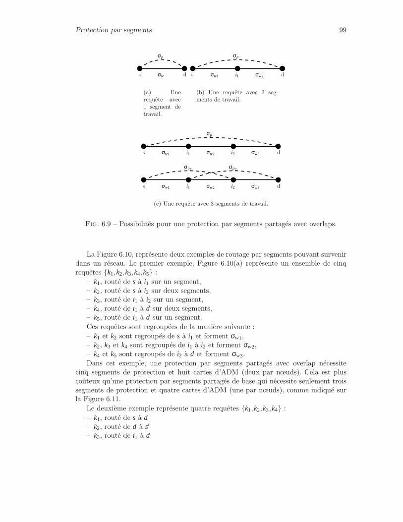
Protection par segments 99
s d
σp
σw
(a) Unerequête avec1 segment detravail.
s d
σp
σw1 i1 σw2
(b) Une requête avec 2 seg-ments de travail.
s d
s d
σp
σw1 i1 σw2 i2 σw3
σp2σp1
σw1 i1 σw2 i2 σw3
(c) Une requête avec 3 segments de travail.
Fig. 6.9 – Possibilités pour une protection par segments partagés avec overlaps.
La Figure 6.10, représente deux exemples de routage par segments pouvant survenirdans un réseau. Le premier exemple, Figure 6.10(a) représente un ensemble de cinqrequêtes k1,k2,k3,k4,k5 :
– k1, routé de s à i1 sur un segment,– k2, routé de s à i2 sur deux segments,– k3, routé de i1 à i2 sur un segment,– k4, routé de i1 à d sur deux segments,– k5, routé de i1 à d sur un segment.Ces requêtes sont regroupées de la manière suivante :– k1 et k2 sont regroupés de s à i1 et forment σw1,– k2, k3 et k4 sont regroupés de i1 à i2 et forment σw2,– k4 et k5 sont regroupés de i2 à d et forment σw3.Dans cet exemple, une protection par segments partagés avec overlap nécessite
cinq segments de protection et huit cartes d’ADM (deux par nœuds). Cela est pluscoûteux qu’une protection par segments partagés de base qui nécessite seulement troissegments de protection et quatre cartes d’ADM (une par nœuds), comme indiqué surla Figure 6.11.
Le deuxième exemple représente quatre requêtes k1,k2,k3,k4 :– k1, routé de s à d– k2, routé de d à s′
– k3, routé de i1 à d

100 Fiabilité et tolérance aux pannes
s dσw3i2σw2i1σw1
(a) Un premier ensemble de routage parsegment.
s d
σw6
σw5 σw4
σw3i2σw2i1σw1
s’
(b) Un second ensemble de routage parsegment.
Fig. 6.10 – Deux types interactions possibles entre des segments de travail.
σp2 σp3σp1
dσw3i2σw2i1σw1s
(a) Sans overlap : trois segments de pro-tection et quatre cartes d’ADM.
σp2 σp3σp1
σp4σp5
s di1 i2 σw3σw2σw1
(b) Avec overlap : cinq segments de pro-tection et huit cartes d’ADM.
Fig. 6.11 – Comparaison des deux protections pour l’exemple de la Figure 6.10(a).
– k4, routé de d à i1Ces requêtes sont routées en formant des segments de travail de la manière suivante :– k1 est routé de s à i1, ce qui forme σp1,– k1 et k3 sont regroupés de i1 à i2, ce qui forme σp2,– k1 et k3 sont regroupés de i2 à d ce qui forme σp3,– k2 et k4 sont regroupés de d à i2 ce qui forme σp4,– k2 et k4 sont regroupés de i2 à i1 ce qui forme σp5,– k2 est routés de i1 à s′ ce qui forme σp6,Dans cet exemple, une protection par segments partagés avec overlap nécessite cinq
cartes d’ADM (une par nœuds), alors qu’une protection par segments partagés de basenécessite sept cartes d’ADM. (deux pour les nœuds i1 et i2, une aux autres nœuds).Cela est représenté sur la Figure 6.12.
6.2.3 Formulations mathématiques
Dans l’Annexe D.2, sont présentées des formulations mathématiques pour ces deuxproblèmes. N. Bhuiyan, de l’université de Concordia, est actuellement en train de lesimplémenter. L’objectif est de comparer les performances de ces formulations avec desalgorithmes déjà existants.

Conclusion et Perspectives 101
σp4σp5
s d
σp1
σp6
σp2 σp3
i2i1
s’
(a) Sans overlap : six segments de pro-tection et sept cartes d’ADM.
s d
σp4
σp2
i2
σp1
i1
σp3
s’
(b) Avec overlap : quatre segments deprotection et cinq cartes d’ADM.
Fig. 6.12 – Comparaison des deux protections pour l’exemple de la Figure 6.10(b).
6.3 Conclusion et Perspectives
Dans ce chapitre, j’ai présenté des problèmes relatifs à la fiabilité des connexionsétablies. Ces problèmes sont essentiels pour satisfaire les clients. La première partieconcerne les risques de pannes multiples. J’y ai présenté un moyen d’en tenir comptelors du routage. L’efficacité de la formulation mathématique proposée est illustrée pardes résultats expérimentaux. Dans la deuxième partie, je présente deux nouveaux typesde protections ; Je présente leur mode de fonctionnement et, ensuite, je les compareentre eux. Les modèles mathématiques correspondants sont en cours d’implémentationet vont permettre de comparer ces types de protections à d’autres déjà existants.
L’étape suivante est de "fusionner" les formulations mathématiques des deux sectionsafin de prendre en compte les risques de pannes multiples lors de la protection derequêtes. Il serait également intéressant d’étendre ces formulations aux multicasts.

102 Fiabilité et tolérance aux pannes

Chapitre 7
Reroutage de connexions etPathwidth
Dans ce chapitre, je présente un invariant de graphe appelé process number quia été introduit pour modéliser les reconfigurations d’un routage d’un réseau WDMdont les ressources ou les requêtes évoluent dynamiquement. Je présente les liensentre cet invariant et d’autres invariants dont la pathwidth. Ensuite, je présenteun algorithme permettant de calculer le process number d’un arbre, ainsi que desavancées sur les liens entre la pathwidth d’un graphe planaire extérieur et cellede son dual (à savoir que pour tout graphe graphe planaire extérieur biconnexe Gsans boucles ni arêtes multiples, on a pw(G∗) ≤ pw(G) ≤ 2pw(G∗)− 1) et sur lesliens entre la pathwidth d’un graphe planaire et celle son dual (pour tout grapheplanaire 3-connexe G, on a 1
3 pw(G∗)−2≤ pw(G) ≤ 3pw(G∗)+ 2). Je finis sur desconsidérations concernant l’indice d’échappement arête connexe.
L’étude de la reconfiguration d’un routage à l’intérieur d’un réseau WDM a mené àintroduire un invariant : le process number, c.f. [CS07]. Dans cette section, je commencepar en rappeler la définition ainsi que celles de paramètres qui lui sont reliés commela pathwidth notamment. Ensuite, je présente les résultats que j’ai obtenus au coursde ma thèse : un algorithme distribué permettant de calculer divers paramètres sur lesarbres, un algorithme d’approximation pour calculer la pathwidth de graphes planairesextérieurs et des avancées sur plusieurs conjectures.
7.1 Origine du problème
Le principe du WDM (Wavelength Division Multiplexing), qui est rappelé en Sec-tion 5.1.1.5, est de permettre à une même fibre optique de transmettre plusieurs lon-gueurs d’onde, augmentant ainsi sa capacité. Un routage dans un réseau WDM est
103

104 Reroutage de connexions et Pathwidth
une affectation à chaque requête d’un chemin et d’une longueur d’onde de telle sorteque deux requêtes dont les chemins partagent une arête aient deux longueurs d’ondedifférentes (c.f. Problème 5.1). Je me restreins ici au cas où il n’y a pas de conversion delongueur d’onde. Cependant, pour tenir compte de la conversion de longueur d’onde,il suffit de partager une requête en plusieurs sous requêtes. Au cours des ajouts et dessuppressions de requêtes dus à l’évolution du trafic, si le routage des requêtes déjàprésentes n’est pas modifié, il se peut que l’on se trouve dans des configurations ne per-mettant plus d’ajouter les nouvelles requêtes alors que les ressources sont suffisantes.Ainsi, il est nécessaire de changer le routage des requêtes présentes dans le réseau detemps en temps. Ce problème est illustré par l’exemple suivant.
Nous considérons une fibre ayant deux longueurs d’onde λ1 et λ2, dans laquelle sonteffectuées les opérations suivantes : routage de la requête A - B sur λ1, routage de larequête A - C sur λ2, routage de la requête B - E sur λ1, routage de la requête D - Esur λ2, suppression de la requête B - E et enfin routage de la requête C - E sur λ1. Lasuccession de ces modifications du trafic est représentée sur la Figure 7.1.
A B C D E
λ1
λ2
A B C D E
λ1
λ2
A B C D E
λ1
λ2
A B C D E
λ1
λ2
A B C D E
λ1
λ2
A B C D E
λ1
λ2
Fig. 7.1 – Exemple d’opérations successives entraînant un blocage.
Le réseau se retrouve dans une configuration telle qu’il n’est pas possible d’ajouterla requête B - D alors que la Figure 7.2 montre qu’un autre routage des requêtes déjàprésentes le permet. Il faudrait déplacer la requête C - E sur λ2 et la requête D - E surλ1. Seulement, pour déplacer ces deux requêtes, il faut interrompre l’une des deux carchacune des requêtes veut prendre la place de l’autre. Pour éviter cette interruption,une solution consiste à utiliser une longueur d’onde supplémentaire λ3 que l’on ne peututiliser que lors de la reconfiguration. On peut alors déplacer la requête C - E sur λ3,la requête D - E sur λ1, la requête C - E sur λ2 et enfin router la requête B - D surλ2. Contrairement à une suppression puis à l’ajout d’une requête, le déplacement d’unerequête peut se faire sans interruption de service.
Nous supposons dans la suite que les longueurs d’onde supplémentaires, que l’on ap-pelle mémoires temporaires (temporary memory units TMU), ne peuvent supporterqu’une seule requête chacune. La question est de savoir quel est le nombre minimumde mémoires temporaires nécessaires pour passer d’un routage à un autre. Si l’on nedispose pas de mémoires temporaires, il s’agit de savoir quel est le nombre minimumde connexions qu’il va falloir arrêter simultanément.
On modélise le changement d’une configuration C à une configuration C′ par un

Origine du problème 105
A B C D EA B C D E
λ1
λ2
λ1
λ2
Fig. 7.2 – Illustration du blocage et solution.
graphe orienté des conflits D comme suit : chaque requête est représentée par unsommet et on met un arc d’un sommet représentant une requête r vers un sommetreprésentant une requête s si dans la configuration C, s utilise une ressource (dansnotre cas, une ressource est une paire lien-longueur d’onde) utilisée par r dans C′. LaFigure 7.3 représente le graphe des conflits dans le cas de l’exemple de la Figure 7.2
C−E D−EB−D
Fig. 7.3 – Exemple de graphe de conflit.
Passer de la configuration C à la configuration C′ en utilisant des mémoires tempo-raires revient à supprimer tous les sommets du graphe orienté auxiliaire en respectantles règles suivantes :
– On peut à tout moment mettre un sommet dans une mémoire temporaire. cefaisant, on supprime tous les arcs entrant de ce sommet.
– On peut supprimer un sommet qui n’a pas d’arc sortant, si le sommet était dansune mémoire temporaire, il la libère.
Une suite d’actions permettant de supprimer tous les sommets d’un graphe orientéD est appelée stratégie de reroutage. Le nombre maximum de mémoires temporairessimultanément utilisées par une stratégie de reroutage est appelé coût de la straté-gie de reroutage, le minimum des coûts des stratégies de reroutage est le processnumber du graphe orienté, on le note pn(D).
Étant donné un graphe (non orienté) G, le process number de G est le processnumber du graphe orienté obtenu de G en remplaçant chaque arête par un circuitorienté de longueur deux, soit deux arcs, un dans chaque direction. Pour la suite, ilest intéressant de remarquer que dans le cas des graphes (simples), cette définitionest équivalente à une définition faisant référence à un jeux tour à tour dans lequel unensemble d’agents souhaitent capturer un fugitif, ou de manière équivalente s’assurerqu’il ne peut se cacher dans aucun sommet.
Le process number d’un graphe est le nombre minimum d’agents nécessaires pourtraiter tous les sommets d’un graphe en respectant les règles suivantes :
– Positionner un agent sur un sommet (on dit d’un sommet sur lequel est positionnéun agent qu’il est occupé par un agent).
– Traiter un sommet encerclé (un sommet tel qu’un agent est positionné sur cha-
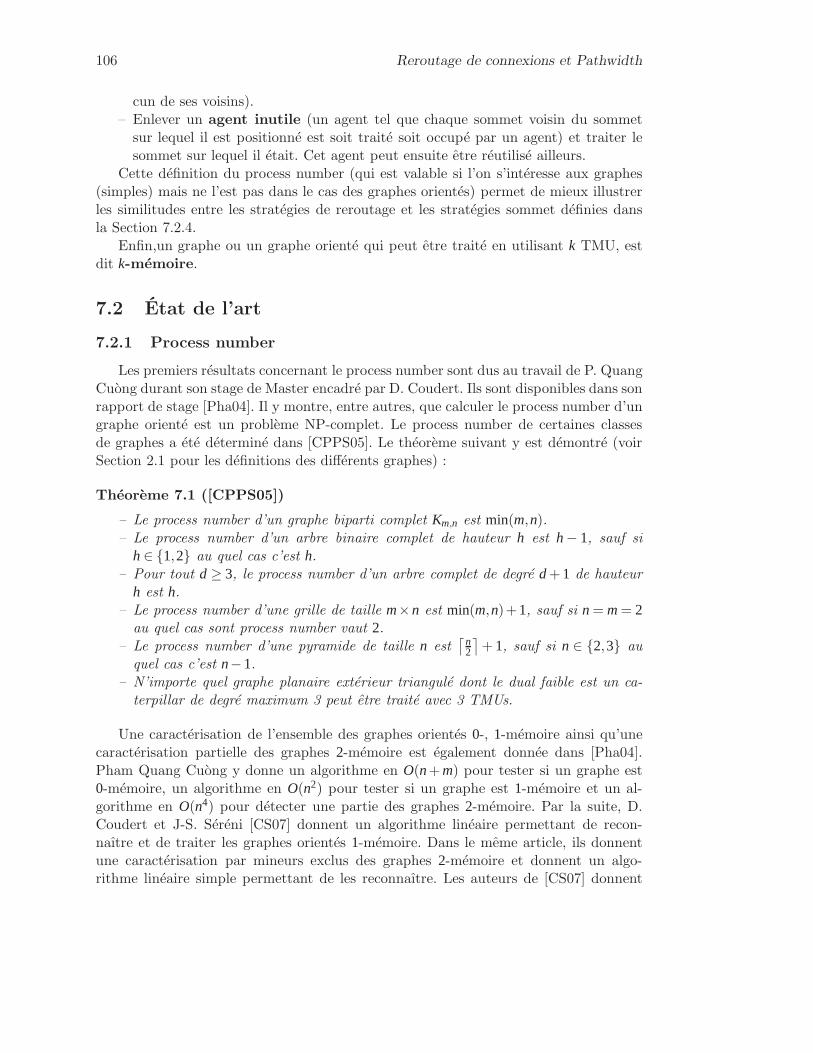
106 Reroutage de connexions et Pathwidth
cun de ses voisins).– Enlever un agent inutile (un agent tel que chaque sommet voisin du sommet
sur lequel il est positionné est soit traité soit occupé par un agent) et traiter lesommet sur lequel il était. Cet agent peut ensuite être réutilisé ailleurs.
Cette définition du process number (qui est valable si l’on s’intéresse aux graphes(simples) mais ne l’est pas dans le cas des graphes orientés) permet de mieux illustrerles similitudes entre les stratégies de reroutage et les stratégies sommet définies dansla Section 7.2.4.
Enfin,un graphe ou un graphe orienté qui peut être traité en utilisant k TMU, estdit k-mémoire.
7.2 État de l’art
7.2.1 Process number
Les premiers résultats concernant le process number sont dus au travail de P. QuangCuòng durant son stage de Master encadré par D. Coudert. Ils sont disponibles dans sonrapport de stage [Pha04]. Il y montre, entre autres, que calculer le process number d’ungraphe orienté est un problème NP-complet. Le process number de certaines classesde graphes a été déterminé dans [CPPS05]. Le théorème suivant y est démontré (voirSection 2.1 pour les définitions des différents graphes) :
Théorème 7.1 ([CPPS05])
– Le process number d’un graphe biparti complet Km,n est min(m,n).– Le process number d’un arbre binaire complet de hauteur h est h− 1, sauf si
h∈ 1,2 au quel cas c’est h.– Pour tout d ≥ 3, le process number d’un arbre complet de degré d+1 de hauteur
h est h.– Le process number d’une grille de taille m×n est min(m,n)+1, sauf si n = m= 2
au quel cas sont process number vaut 2.– Le process number d’une pyramide de taille n est
⌈
n2
⌉
+ 1, sauf si n ∈ 2,3 auquel cas c’est n−1.
– N’importe quel graphe planaire extérieur triangulé dont le dual faible est un ca-terpillar de degré maximum 3 peut être traité avec 3 TMUs.
Une caractérisation de l’ensemble des graphes orientés 0-, 1-mémoire ainsi qu’unecaractérisation partielle des graphes 2-mémoire est également donnée dans [Pha04].Pham Quang Cuòng y donne un algorithme en O(n+ m) pour tester si un graphe est0-mémoire, un algorithme en O(n2) pour tester si un graphe est 1-mémoire et un al-gorithme en O(n4) pour détecter une partie des graphes 2-mémoire. Par la suite, D.Coudert et J-S. Séréni [CS07] donnent un algorithme linéaire permettant de recon-naître et de traiter les graphes orientés 1-mémoire. Dans le même article, ils donnentune caractérisation par mineurs exclus des graphes 2-mémoire et donnent un algo-rithme linéaire simple permettant de les reconnaître. Les auteurs de [CS07] donnent
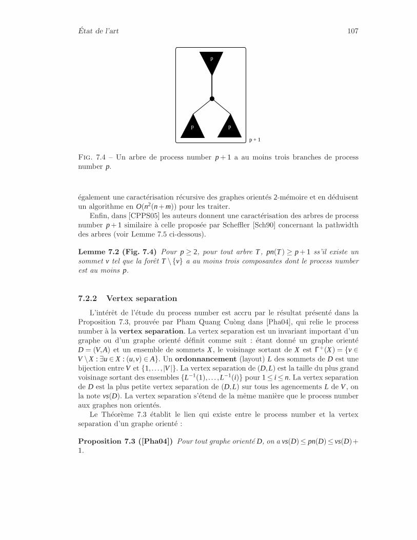
État de l’art 107
p
p
p
p + 1
Fig. 7.4 – Un arbre de process number p+ 1 a au moins trois branches de processnumber p.
également une caractérisation récursive des graphes orientés 2-mémoire et en déduisentun algorithme en O(n2(n+m)) pour les traiter.
Enfin, dans [CPPS05] les auteurs donnent une caractérisation des arbres de processnumber p+ 1 similaire à celle proposée par Scheffler [Sch90] concernant la pathwidthdes arbres (voir Lemme 7.5 ci-dessous).
Lemme 7.2 (Fig. 7.4) Pour p≥ 2, pour tout arbre T, pn(T) ≥ p+ 1 ss’il existe unsommet v tel que la forêt T \v a au moins trois composantes dont le process numberest au moins p.
7.2.2 Vertex separation
L’intérêt de l’étude du process number est accru par le résultat présenté dans laProposition 7.3, prouvée par Pham Quang Cuòng dans [Pha04], qui relie le processnumber à la vertex separation. La vertex separation est un invariant important d’ungraphe ou d’un graphe orienté définit comme suit : étant donné un graphe orientéD = (V,A) et un ensemble de sommets X, le voisinage sortant de X est Γ+(X) = v ∈V \X : ∃u∈ X : (u,v) ∈ A. Un ordonnancement (layout) L des sommets de D est unebijection entre V et 1, . . . , |V|. La vertex separation de (D,L) est la taille du plus grandvoisinage sortant des ensembles L−1(1), . . . ,L−1(i) pour 1≤ i ≤ n. La vertex separationde D est la plus petite vertex separation de (D,L) sur tous les agencements L de V, onla note vs(D). La vertex separation s’étend de la même manière que le process numberaux graphes non orientés.
Le Théorème 7.3 établit le lien qui existe entre le process number et la vertexseparation d’un graphe orienté :
Proposition 7.3 ([Pha04]) Pour tout graphe orienté D, on a vs(D)≤ pn(D)≤ vs(D)+1.

108 Reroutage de connexions et Pathwidth
Dans [CS07], D. Coudert et J-S. Séréni donnent un critère permettant de décider sipour un graphe orienté D on a pn(D) = vs(D)+1 :
Proposition 7.4 ([CS07]) Pour tout graphe orienté D, il existe une stratégie de re-routage utilisant pn(D) TMU et telle que tout sommet est placé en TMU ssi pn(D) =vs(D)+1.
Cependant ce critère nécessite de connaître une stratégie de reroutage optimale etde savoir vérifier si elle peut être transformée de telle sorte que tout sommet soit placéen TMU.
7.2.3 Pathwidth
Dans le cas des graphes, Kinnersley a prouvé que la vertex separation d’un grapheest égale à sa pathwidth (notée pw(G)), qui est un autre paramètre introduit parRobertson et Seymour [RS83]. Pour définir ce paramètre, j’ai besoin d’introduire ladécomposition en chemins d’un graphe G = (V,E). C’est un ensemble d’ensembles(X1, . . . ,Xr) de V tels que :
1.Sr
i=1 Xi = V
2. ∀xy∈ E,∃i ∈ 1, . . . , r : x,y ⊂ Xi
3. pour tout 1≤ i0 < i1 < i2 ≤ r, Xi0 ∩Xi2 ⊆ Xi1
La largeur de la décomposition en chemins (X1, . . . ,Xr) est max1≤i≤r |Xi|−1. La path-width de G, notée pw(G), est la largeur minimale des décompositions en chemins.
Le calcul de la pathwidth d’un graphe est un domaine de recherche actif dans lequelbeaucoup de travail a été fait. Le lecteur intéressé pourra se référer au survey de B.Reed [Ree97].
On notera, entre autres, qu’il existe un algorithme linéaire permettant de calculerla pathwidth d’un arbre [Sch90]. Cet algorithme est basé sur la caractérisation suivantedes arbres de pathwidth p+1 :
Lemme 7.5 ([Sch90]) Pour tout arbre T, pw(T) ≥ p+ 1 s’il existe un sommet v telque la forêt T \v ait au moins trois composantes dont la pathwidth est au moins p.
Ce même algorithme permet d’obtenir une décomposition en chemins optimale entemps O(nlog(n)). Ce résultat a été amélioré par K. Skodinis qui propose dans [Sko00],un algorithme permettant d’obtenir un ordonnancement des sommets optimal par rap-port à la vertex separation en temps linéaire.
7.2.4 Indice d’échappement sommet
La vertex separation et donc la pathwidth sont également équivalents à l’indiced’échappement sommet (node search number en anglais), un autre invariant impor-tant introduit par L.M. Kirousis et C.H. Papadimitriou dans [KP86] dans le cadre desjeux de recherche. Les jeux de recherches sont des jeux qui opposent tour à tour un
État de l’art 109
fugitif à des agents. Le but de ces jeux est de déterminer le nombre minimum d’agentsnécessaires pour capturer le fugitif dans un graphe sous certaines conditions de dépla-cement des agents et du fugitif. Dans le cadre d’une stratégie sommet, le fugitif a ledroit, à son tour, de se déplacer d’autant d’arêtes qu’il veut dans le graphe tant qu’il nepasse pas par un sommet occupé par un agent. Ensuite, au tour des agents, l’un d’euxpeut faire une des deux actions suivantes :
– se positionner sur un sommet s’il n’est pas déjà positionné sur un autre sommet.Le sommet est dit occupé.
– se retirer d’un sommet sur lequel il est positionné afin de pouvoir se positionnersur un autre sommet lors d’un prochain tour.
Le fugitif est capturé s’il se trouve sur un sommet occupé par un agent ou sur unearête dont les deux extrémités sont occupées par un agent. Étant donné un grapheG, le nombre minimum d’agents nécessaires pour capturer le fugitif (invisible pour lesagents tant qu’il n’a pas été capturé) quels que soit ses mouvements est appelé l’indiced’échappement sommet. Il est noté sn(G).
Remarque 7.6 L’indice d’échappement sommet peut aussi être vu comme le nombred’agents nécessaires pour nettoyer tous les sommets d’un graphe de telle sorte qu’initialement tous les sommets soient contaminés et qu’un sommet non occupé par unagent est recontaminé s’il est adjacent à un sommet contaminé. Un sommet contaminéreprésente un sommet sur lequel le fugitif peut se trouver.
Remarque 7.7 Selon une remarque de S. Thomassé, si l’on rajoute la règle que lefugitif ne peut pas rester immobile (ce qui peut être simulé par la présence d’un chienaidant les policiers), la nouvelle version de l’indice d’échappement sommet obtenuedonne le process number. En effet, pour obtenir la règle que les sommets encerclés sontnettoyés, il suffit que les policiers ne bougent qu’un tour sur deux.
Comme N. Nisse dans [Nis07], on appelle une suite de déplacements des policierspermettant de capturer le fugitif quelque soit ses déplacements, une stratégie decapture sommet.
Dans [EST94], J.A. Ellis, I.H. Sudborough et J. Türner montrent que l’indiced’échappement sommet d’un graphe est égal à sa pathwidth plus un : sn(G) = pw(G)+1.
De plus on peut noter qu’il existe une suite de O(n) mouvements permettant decapturer le fugitif car recontaminer une partie du graphe, c.à.d. laisser la possibilitéau fugitif de revenir sur un sommet qui a déjà été occupé par un agent, ne permet pasd’utiliser moins d’agents. Ceci est un résultat de A. S. LaPaugh : [LaP93].
Du fait que la recontamination n’aide pas, on peut aussi déduire que si on autoriseun agent à se retirer d’un sommet uniquement s’il est inutile (dans le même sens quepour le process number, c.à.d. si chaque sommet voisin au sommet qu’il occupe estsoit occupé par un agent soit l’a déjà été) alors le nombre d’agents nécessaires pourcapturer le fugitif n’augmente pas. Dans ce cas, les agents suivent les mêmes règles dedéplacements que lors du calcul du process number des graphes simples. La différenceréside dans le fait que dans une stratégie sommet, on ne peut pas considérer comme

110 Reroutage de connexions et Pathwidth
traité un noeud entouré par des agents. Autrement dit, dans le cas d’une stratégiesommet, tous les sommets doivent être visités par un agent.
Ces dernières années de nombreux travaux ont vu le jour sur différentes variantesdes jeux de recherche. Le lecteur intéressé pourra lire le survey récemment écrit par F.Fomin et D. Thilikos [FT08] ainsi que la thèse de N. Nisse [Nis07].
J’évoque deux variantes intéressantes. La première est le cas où le fugitif est visible,dans ce cas le nombre d’agents nécessaires à sa capture donne la treewidth. La deuxièmevariante est quand les agents peuvent demander un nombre limité de fois la positiondu fugitif. Cette variante donne toute une famille d’intermédiaire entre la pathwidth etla treewidth.
Par la suite, je me contente de présenter les définitions et les résultats dont j’aibesoin.
7.2.5 Indice d’échappement arête
Une stratégie arête est une variante d’une stratégie sommet dans laquelle les po-liciers, en plus des déplacements autorisés dans le cadre des stratégies sommet, peuventse déplacer le long d’une arête. Dans cette variante, le fugitif est capturé si un agentest sur le même sommet que lui ou si un agent traverse l’arête dans laquelle il est.
Dans le cadre d’une stratégie arête, on appelle une suite de déplacements permettantde capturer le fugitif une stratégie de capture arête. Étant donné un graphe G, lenombre minimum d’agents nécessaires à une stratégie de capture arête dans G estl’indice d’échappement arête (edge search number), on le note es(G).
Remarque 7.8 L’indice d’échappement arête peut aussi être vu comme le nombred’agents nécessaires pour nettoyer tous les sommets et toutes les arêtes d’un graphe detelle sorte qu’initialement tout le graphe est contaminé et qu’un sommet non occupé parun agent est recontaminé s’il est adjacent à un élément (sommet ou arête) contaminé,de même pour les arêtes si un de leur sommet non occupé est adjacent à un élémentcontaminé. Un élément contaminé représente un élément sur lequel le fugitif peut setrouver.
En utilisant un agent supplémentaire, il est facile de transformer une stratégie decapture arête en une stratégie de capture sommet et vice versa. En effet, un agent qui sedéplace le long d’une arête dans une stratégie de capture arête peut être remplacé pardeux agents, un à chaque extrémité de l’arête, dans une stratégie de capture sommet.Pour passer d’une stratégie de capture sommet à une stratégie de capture arête, ilsuffit d’utiliser un agent supplémentaire pour visiter chaque arête quand des agentssont positionnés sur ses extrémités.
Ainsi, on obtient que pour tout graphe G :
es(G)−1≤ ns(G) ≤ es(G)+1.

État de l’art 111
7.2.6 Indice d’échappement arête connexe
On peut aussi citer la variante de la stratégie arête proposée par P. Fraigniaud et aldans [BFFS02] : la stratégie arête connexe (contiguous search number). Dans cettevariante, la zone dans laquelle le fugitif ne peut pas se trouver, appelée zone sûre, doitêtre connexe. Ils proposent également une variante pondérée de ce jeu de recherche.Dans la variante pondérée, le poids d’une arête ou d’un sommet indique le nombred’agents nécessaires pour nettoyer cette arête ou ce sommet. Enfin un sommet doitêtre gardé par un nombre d’agents supérieur au poids de chaque arête adjacente afind’empêcher toute recontamination. Une stratégie permettant de capturer à coup sûrun fugitif, est appelée une stratégie capture arête connexe
Le nombre minimum d’agents nécessaires pour capturer un fugitif dans un graphe Gest appelé indice d’échappement arête connexe de G (contiguous search number)et est noté cs(G).
Dans [BFFS02], les auteurs présentent un algorithme linéaire permettant de calculerl’indice d’échappement arête connexe cs(T) d’un arbre pondéré (T,w). Cet algorithmerepose sur le Lemme 7.9. Étant donné un arbre de racine u et un noeud v, on note Tu lesous-arbre maximal connexe de racine u ne contenant pas d’arêtes du chemin de u à v.
Lemme 7.9 Étant donné un arbre pondéré (T,w) de racine y où w est une fonction deV ∪E → N, si y1, . . . ,yp sont les fils de y tels que cs(Tyi ) ≥ cs(Tyi+1) pour 1≤ i < p, alorscs(T) = max(cs(Ty1),cs(Ty2)+w(y2)).
Dans le cas non pondéré, ce lemme est exact car on peut montrer que, traiter unsous-arbre Tyi partiellement avant d’en traiter un autre n’aide pas. Par contre, dans lecas pondéré, ce lemme est incorrect comme l’illustre l’exemple de la Figure 7.5. L’erreurprovient du fait que, dans le cas où les agents sont positionnés sur le sommet y, il estmoins coûteux d’envoyer un seul agent garder le sommet y1 avant de nettoyer l’arbreTy2 plutôt que de laisser 10 agents sur y afin de le garder pendant que l’on nettoie Ty2.
y
y1 y2
1 10
10
10
1015
1
1
Fig. 7.5 – Contre exemple au Lemme 7.9.
Cet exemple permet de construire un arbre (cf Figure 7.6) pour lequel l’algorithmeprésenté dans [BFFS02] renvoie une valeur fausse : 16 au lieu de 15.
Dans la Section 7.3.4, je présente de nouveaux résultats concernant cette variantede l’indice d’échappement arête.
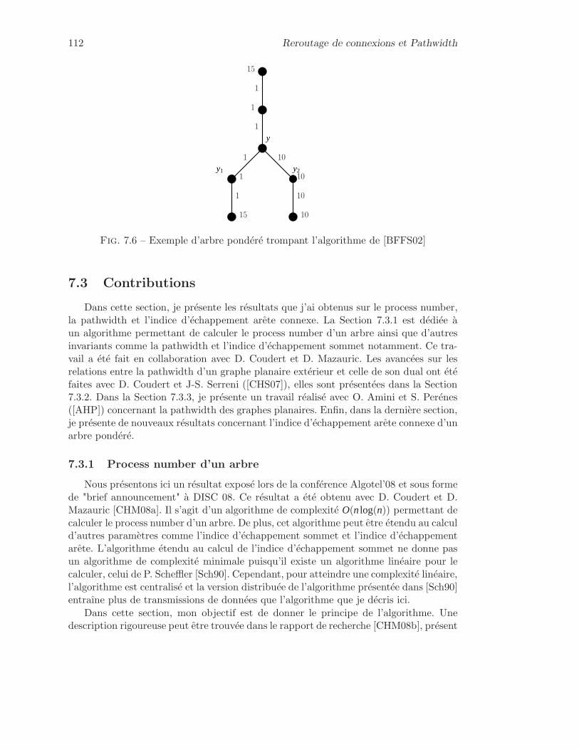
112 Reroutage de connexions et Pathwidth
y1 y2
1 10
10
10
1015
1
1
y1
1
1
15
Fig. 7.6 – Exemple d’arbre pondéré trompant l’algorithme de [BFFS02]
7.3 Contributions
Dans cette section, je présente les résultats que j’ai obtenus sur le process number,la pathwidth et l’indice d’échappement arête connexe. La Section 7.3.1 est dédiée àun algorithme permettant de calculer le process number d’un arbre ainsi que d’autresinvariants comme la pathwidth et l’indice d’échappement sommet notamment. Ce tra-vail a été fait en collaboration avec D. Coudert et D. Mazauric. Les avancées sur lesrelations entre la pathwidth d’un graphe planaire extérieur et celle de son dual ont étéfaites avec D. Coudert et J-S. Serreni ([CHS07]), elles sont présentées dans la Section7.3.2. Dans la Section 7.3.3, je présente un travail réalisé avec O. Amini et S. Perénes([AHP]) concernant la pathwidth des graphes planaires. Enfin, dans la dernière section,je présente de nouveaux résultats concernant l’indice d’échappement arête connexe d’unarbre pondéré.
7.3.1 Process number d’un arbre
Nous présentons ici un résultat exposé lors de la conférence Algotel’08 et sous formede "brief announcement" à DISC 08. Ce résultat a été obtenu avec D. Coudert et D.Mazauric [CHM08a]. Il s’agit d’un algorithme de complexité O(nlog(n)) permettant decalculer le process number d’un arbre. De plus, cet algorithme peut être étendu au calculd’autres paramètres comme l’indice d’échappement sommet et l’indice d’échappementarête. L’algorithme étendu au calcul de l’indice d’échappement sommet ne donne pasun algorithme de complexité minimale puisqu’il existe un algorithme linéaire pour lecalculer, celui de P. Scheffler [Sch90]. Cependant, pour atteindre une complexité linéaire,l’algorithme est centralisé et la version distribuée de l’algorithme présentée dans [Sch90]entraîne plus de transmissions de données que l’algorithme que je décris ici.
Dans cette section, mon objectif est de donner le principe de l’algorithme. Unedescription rigoureuse peut être trouvée dans le rapport de recherche [CHM08b], présent
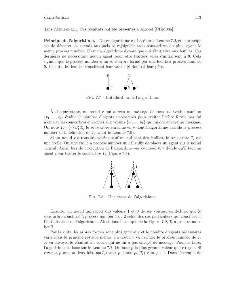
Contributions 113
dans l’Annexe E.1. Ces résultats ont été présentés à Algotel [CHM08a].
Principe de l’algorithme. Notre algorithme est basé sur le Lemme 7.2, et le principeest de détecter les nœuds auxquels se rejoignent trois sous-arbres ou plus, ayant lemême process number. C’est un algorithme dynamique qui s’initialise aux feuilles. Cesdernières ne nécessitant aucun agent pour être traitées, elles s’initialisent à 0. Celasignifie que le process number d’un sous-arbre formé par une feuille a process number0. Ensuite, les feuilles transfèrent leur valeur (0 donc) à leur père.
0 0 0
Fig. 7.7 – Initialisation de l’algorithme.
À chaque étape, un nœud v qui a reçu un message de tous ses voisins sauf unv1, . . . ,vk évalue le nombre d’agents nécessaires pour traiter l’arbre formé par luimême et les sous-arbres enracinés aux voisins v1, . . . ,vk qui lui ont envoyé un message.On note Tv= v∪k
1 Tvi le sous-arbre enraciné en v dont l’algorithme calcule le processnumber (c.f. définition de Tv avant le Lemme 7.9).
Si un nœud v a tous ses voisins sauf un qui sont des feuilles, le sous-arbre Tv estune étoile. Or, une étoile a process number un : il suffit de placer un agent sur le nœudcentral. Ainsi, lors de l’éxécution de l’algorithme sur ce nœud v, v décide qu’il faut unagent pour traiter le sous-arbre Tv (Figure 7.8).
v v
11
Fig. 7.8 – Une étape de l’algorithme.
Ensuite, un nœud qui reçoit des valeurs 1 et 0 de ses voisins, va déduire que lesous-arbre constitué à process number 1 ou 2 selon des cas particuliers qui constituentl’initialisation de l’algorithme. Ainsi dans l’exemple de la Figure 7.9, Tv a process num-ber 2.
Par la suite, les arbres formés sont plus généraux et le nombre d’agents nécessairesvarie mais le principe reste le même. Un nœud v va calculer le process number de Tv
et va envoyer le résultat au voisin qui ne lui a pas envoyé de message. Pour ce faire,l’algorithme se base sur le Lemme 7.2. On note p la plus grande valeur que v reçoit. Siv reçoit p une ou deux fois, pn(Tv) vaut p, sinon pn(Tv) vaut p+1. Dans l’exemple de

114 Reroutage de connexions et Pathwidth
v
2
Fig. 7.9 – Le process number de Tv vaut 2.
la Figure 7.10, le nœud v0 reçoit deux fois la valeur 2 et le process number de Tv0 vautbien 2.
2 2
v2
v0
v1
Fig. 7.10 – Le process number de Tv0 vaut 2.
Je continue à décrire le déroulement de cet algorithme sur l’arbre T de la Figure 7.11.
Nous avons vu que les nœuds v0 et v3 calculent que pn(Tv0) et pn(Tv3) valent tousles deux 2 (Figures 7.8 et 7.10). v0 et v3 envoient donc tous les deux la valeur 2 à u quicalcule Tu. Selon les règles précédentes, comme u reçoit deux fois la valeur 2, il déduitque pn(Tu) (et donc pn(T)) vaut 2, or c’est faux : pn(T) = 3.

Contributions 115
v3 v2
u v0
v1
Fig. 7.11 – Le process number de T vaut 3 et non 2.
Origine de l’erreur. L’erreur vient du fait que le nœud u n’a pas détecté que v0 atrois voisins qui sont racines de sous-arbres de process number 2 : Tv1 et Tv2 dont il areçu le process number et Tu dont le process number n’avait pas encore été calculé parl’algorithme au moment où v0 a fait son calcul.
Pour éviter cette erreur, étant donné un nœud v qui reçoit des informations de tousses voisins sauf un, on distingue trois cas qui peuvent se produire :
1. parmi les voisins v1, . . . ,vk dont v reçoit un message, seul l’un d’eux est racined’un sous-arbre de process number maximal : p = pn(Tv1) > pn(Tvi ),1 < i ≤ k ;
2. parmi les voisins v1, . . . ,vk dont v reçoit un message, deux sont racines d’unsous-arbre de process number maximal : p= pn(Tv1) = pn(Tv2) > pn(Tvi ),2< i ≤ k ;
3. parmi les voisins v1, . . . ,vk dont v reçoit un message, au moins trois sont racinesd’un sous-arbre de process number maximal : p = pn(Tv1) = pn(Tv2) = pn(Tv3) ≥pn(Tvi ),3 < i ≤ k.
pq
p
pp
?=p ou p+1
pp p
p+1
Fig. 7.12 – Trois cas de figure possibles.

116 Reroutage de connexions et Pathwidth
Dans le premier cas, d’après le Lemme 7.2, on sait qu’il y a deux sous-arbres qui sontdéterminants : le sous-arbre qui n’a pas encore été exploré (qui est celui qui correspondau voisin n’ayant pas envoyé de message) et le sous-arbre enraciné en v1 (qui est celuiavec le plus grand process number (p) parmi ceux qui ont été explorés par l’algorithme).On appelle Tv1 le sous-arbre dominant. On sait que le process number de tout l’arbreT sera le maximum entre le process number de ces deux sous-arbres. Ainsi le nœudcourant v peut envoyer au voisin, dont il n’a pas reçu de message, le process numberdu sous-arbre dominant : p.
Dans le troisième cas, on sait d’après le Lemme 7.2 que l’arbre Tv a process numberp+1. Comme pour le cas précédent, le process number de l’arbre T va être le maximunentre le process number de Tv et le process number du sous-arbre qui n’a pas encoreété exploré. Le nœud courant v peut donc envoyer p+1 au voisin dont il n’a pas reçude message.
Dans le deuxième cas, c’est un peu plus complexe. En effet, on ne sait pas si deuxou trois sous-arbres ayant le même process number p se rejoignent en v car cela dépenddu sous-arbre qui n’a pas encore été exploré. Le process number de l’arbre T peut valoirp (si le sous-arbre qui n’a pas été exploré a un process number plus petit), p+ 1 (sile sous-arbre qui n’a pas été exploré a un process number p) ou le process number dusous-arbre qui n’a pas été exploré s’il est plus grand que p. Pour différencier les troiscas, il est nécessaire d’envoyer plus d’informations que seulement p : il faut signaler quedeux branches de process number p se rejoignent en v.
Un nouvel algorithme. La solution que nous avons adoptée revient à envoyer lemessage "p ou p+1?" et à commencer un nouveau compteur à partir du voisin qui n’apas encore été exploré.
pp
p, p+122
(2,3)
Fig. 7.13 – "p ou p+1?"
Seulement, ce problème peut se poser de manière récursive et on peut être amenéà avoir plusieurs compteurs en parallèle. Les compteurs indiquent des embranchementsde deux types : instables s’ils sont issus d’un nœud étant dans le deuxième cas (ilssont alors du type "p ou p+1?"), et stable s’ils sont issus d’un nœud dans le premierou le troisième cas (ils sont alors du type p).
Les nœuds instables délimitent des sous-arbres et induisent une décomposition denotre arbre initial. Les sous-arbres enracinés à un nœud instable sont représentés pardes rectangles et appelés instables. Les sous-arbres enracinés à un nœud stable sont

Contributions 117
représentés par des triangles et appelés stables. Dans [CHM08b], nous montrons qu’ilest possible d’avoir une décomposition dans laquelle il y a au plus un sous-arbre stable.L’ensemble des compteurs est stocké sous la forme d’un tableau et d’un entier pourl’éventuel sous-arbre stable. Les Figures 7.14, 7.15 et 7.16 donnent trois exemples diffé-rents. Dans notre algorithme, chaque nœud transmet donc un tableau contenant l’en-semble des compteurs. Ces données représentent également la décomposition de Tv ensous-arbres.
(3,4)
(2,3)
(3,4)(4,5)
0*(1,2) 1*(2,3) 2*(3,4) 1*(4,5)
Fig. 7.14 – Premier exemple de décomposition induite par l’algorithme.
2
(8,9)
(5,6)
2 , 0*(1,2) 0*(2,3) 0*(3,4) 0*(4,5) 1*(5,6) 0*(6,7) 0*(7,8) 1*(8,9)
Fig. 7.15 – Deuxième exemple de décomposition induite par l’algorithme.
2
(7,8)
(6,7)
2 , 0*(1,2) 0*(2,3) 0*(3,4) 0*(4,5) 0*(5,6) 1*(6,7) 1*(7,8)
Fig. 7.16 – Troisième exemple de décomposition induite par l’algorithme.
Dans [CHM08b], nous montrons le théorème suivant qui permet de calculer le pro-cess number d’un arbre étant donné une décomposition calculée par l’algorithme :
Théorème 7.10 Etant donné un arbre T et un nœud v, le process number du sous-arbre Tv est égal à la longueur du tableau ℓ calculé par l’algorithme en v si, dans letableau, la dernière série de 1 est précédée d’un 0. Il vaut ℓ+1 sinon.
Pour les trois exemples des Figures 7.14, 7.15 et 7.16 le Théorème 7.10 donne :
Figure 7.14 : 2 , 0*(1,2) 1*(2,3) 2*(3,4) 1*(4,5)
Le process number de l’arbre est 5.
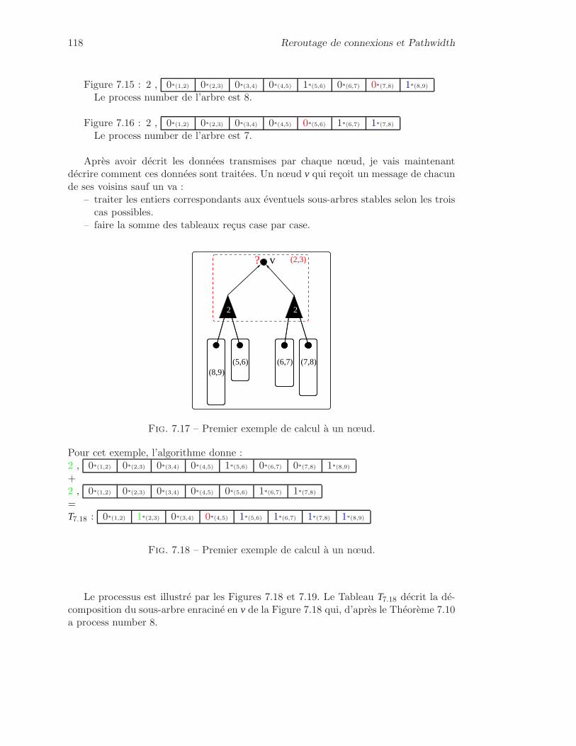
118 Reroutage de connexions et Pathwidth
Figure 7.15 : 2 , 0*(1,2) 0*(2,3) 0*(3,4) 0*(4,5) 1*(5,6) 0*(6,7) 0*(7,8) 1*(8,9)
Le process number de l’arbre est 8.
Figure 7.16 : 2 , 0*(1,2) 0*(2,3) 0*(3,4) 0*(4,5) 0*(5,6) 1*(6,7) 1*(7,8)
Le process number de l’arbre est 7.
Après avoir décrit les données transmises par chaque nœud, je vais maintenantdécrire comment ces données sont traitées. Un nœud v qui reçoit un message de chacunde ses voisins sauf un va :
– traiter les entiers correspondants aux éventuels sous-arbres stables selon les troiscas possibles.
– faire la somme des tableaux reçus case par case.
2 2
v
(7,8)(6,7)(8,9)
? (2,3)
(5,6)
Fig. 7.17 – Premier exemple de calcul à un nœud.
Pour cet exemple, l’algorithme donne :2 , 0*(1,2) 0*(2,3) 0*(3,4) 0*(4,5) 1*(5,6) 0*(6,7) 0*(7,8) 1*(8,9)
+2 , 0*(1,2) 0*(2,3) 0*(3,4) 0*(4,5) 0*(5,6) 1*(6,7) 1*(7,8)
=T7.18 : 0*(1,2) 1*(2,3) 0*(3,4) 0*(4,5) 1*(5,6) 1*(6,7) 1*(7,8) 1*(8,9)
Fig. 7.18 – Premier exemple de calcul à un nœud.
Le processus est illustré par les Figures 7.18 et 7.19. Le Tableau T7.18 décrit la dé-composition du sous-arbre enraciné en v de la Figure 7.18 qui, d’après le Théorème 7.10a process number 8.

Contributions 119
Le Tableau T7.19 décrit la décomposition du sous-arbre enraciné en v de la Fi-gure 7.19. Le Théorème 7.10 dit qu’il a process number 8.
2 2
(4,5)
(3,4)
(2,3)
? v
(8,9)
(5,6) (6,7) (7,8)
(2,3)
Pour cet exemple, l’algorithme donne :2 , 0*(1,2) 1*(2,3) 1*(3,4) 1*(4,5)
+2 , 0*(1,2) 0*(2,3) 0*(3,4) 0*(4,5) 1*(5,6) 0*(6,7) 0*(7,8) 1*(8,9)
+2 , 0*(1,2) 0*(2,3) 0*(3,4) 0*(4,5) 0*(5,6) 1*(6,7) 1*(7,8)
=T7.19 : 0*(1,2) 2*(2,3) 1*(3,4) 1*(4,5) 1*(5,6) 1*(6,7) 1*(7,8) 1*(8,9)
Fig. 7.19 – Deuxième exemple de calcul à un nœud.
Simplification. Si dans un tableau t calculé, il y a une série de cases : de la case kà la case l , remplies de 1 : ∀i,k ≤ i ≤ l , t[i] = 1 et que la case k−1 ne contient pas un0, alors on peut simplifier la décomposition. Étant donné une série de telles cases telleque l soit maximum, toutes les cases d’indice inférieure ou égale à l sont mises à 0 etl’entier décrivant un embranchement stable est mis à l +1. Selon ce principe, le tableauT7.19 correspondant à la Figure 7.19 est simplifié à :
9 , 0*(1,2) 0*(2,3) 0*(3,4) 0*(4,5) 0*(5,6) 0*(6,7) 0*(7,8) 0*(8,9) 0*(9,10)
Cette simplification est justifiée par le Théorème 7.10. Il est montré dans [CHM08b]que ces deux décompositions sont équivalentes. La dernière étant plus simple, notrealgorithme la favorise.
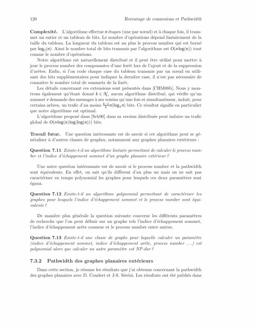
120 Reroutage de connexions et Pathwidth
Complexité. L’algorithme effectue n étapes (une par nœud) et à chaque fois, il trans-met un entier et un tableau de bits. Le nombre d’opérations dépend linéairement de lataille du tableau. La longueur du tableau est au plus le process number qui est bornépar log3(n). Ainsi le nombre total de bits transmis par l’algorithme est O(nlog(n)) toutcomme le nombre d’opérations.
Notre algorithme est naturellement distribué et il peut être utilisé pour mettre àjour le process number des composantes d’une forêt lors de l’ajout et de la suppressiond’arêtes. Enfin, si l’on code chaque case du tableau transmis par un nœud en utili-sant des bits supplémentaires pour indiquer la dernière case, il n’est pas nécessaire deconnaître le nombre total de sommets de la forêt.
Les détails concernant ces extensions sont présentés dans [CHM08b]. Nous y mon-trons également qu’étant donné k ∈ N , aucun algorithme distribué, qui vérifie qu’unsommet v demande des messages à ses voisins qu’une fois et simultanément, induit, pourcertains arbres, un trafic d’au moins k−1
k n(log3n) bits. Ce résultat signifie en particulierque notre algorithme est optimal.
L’algorithme proposé dans [Sch90] dans sa version distribuée peut induire un traficglobal de O(nlog(n) log(log(n))) bits.
Travail futur. Une question intéressante est de savoir si cet algorithme peut se gé-néraliser à d’autres classes de graphes, notamment aux graphes planaires extérieurs :
Question 7.11 Existe-t-il un algorithme linéaire permettant de calculer le process num-ber et l’indice d’échappement sommet d’un graphe planaire extérieur ?
Une autre question intéressante est de savoir si le process number et la pathwidthsont équivalents. En effet, on sait qu’ils diffèrent d’au plus un mais on ne sait pascaractériser en temps polynomial les graphes pour lesquels ces deux paramètres sontégaux.
Question 7.12 Existe-t-il un algorithme polynomial permettant de caractériser lesgraphes pour lesquels l’indice d’échappement sommet et le process number sont équi-valents ?
De manière plus générale la question suivante concerne les différents paramètresde recherche que l’on peut définir sur un graphe tels l’indice d’échappement sommet,l’indice d’échappement arête connexe et le process number entre autres.
Question 7.13 Existe-t-il une classe de graphe pour laquelle calculer un paramètre(indice d’échappement sommet, indice d’échappement arête, process number . . .) estpolynomial alors que calculer un autre paramètre est NP-dur ?
7.3.2 Pathwidth des graphes planaires extérieurs
Dans cette section, je résume les résultats que j’ai obtenus concernant la pathwidthdes graphes planaires avec D. Coudert et J-S. Séréni. Les résultats ont été publiés dans

Contributions 121
Journal of Graph Theory [CHS07], l’article est présent dans l’Annexe E.2. Les défini-tions de graphe planaire, graphe planaire extérieur, dual et dual faible sont rappeléesdans la Section 2.1.
Dans [BF02], H. Bodlaender et F. Fomin ont montré que la pathwidth d’un grapheplanaire extérieur biconnexe est au plus deux fois la pathwidth de son dual plus deux. Ilsont ensuite conjecturé l’existence d’une constante c telle que pour tout graphe planairebiconnexe, sa pathwidth est au plus la pathwidth de son dual plus c. Ils ont égalementconjecturé que c’est vrai pour c = 1. Il est intéressant de noter que cette conjecture apu être motivée par le théorème de D. Lapoire sur la treewidth [Lap99] :
Théorème 7.14 ([Lap99]) Pour tout graphe planaire G, tw(G) ≤ tw(G∗).
Dans [Fom03], F. Fomin montre que la plus forte des conjectures est vraie pour toutetriangulation planaire, mais dans [CHS07], nous montrons que les deux conjectures sontfausses dans le cas général en proposant une famille de graphes planaires extérieursbiconnexes de pathwidth 2p+1 et dont le dual a pathwidth p+2. On montre ensuitede manière algorithmique que cet écart est le plus grand que l’on puisse obtenir. Ondonne ainsi un algorithme de 2-approximation pour calculer la pathwidth des graphesplanaires extérieurs biconnexes. Ces deux résultats sont résumés par les Théorèmes 7.15et 7.16.
Théorème 7.15 Pour tout entier p≥ 1 et tout entier k∈ 1,2, . . . , p+1, il existe ungraphe planaire extérieur biconnexe de pathwidth p+k dont le dual a pathwidth p+1.
Pour prouver ce théorème on utilise une famille de graphes construite récursive-ment à l’aide d’une croix (Figure 7.20(a)). La construction est illustrée par les Fi-gures 7.20(b), 7.20(c) et 7.20(d).
Dans [CHS07], nous prouvons que la pathwidth de ces graphes augmente de deuxà chaque fois (pw(Gi+1) = pw(Gi)+2) alors que celle de leur dual n’augmente que d’un(pw(G∗
i+1) = pw(G∗i )+2). Notre preuve utilise fortement la structure de ces graphes pour
montrer que leur pathwidth augmente de deux à chaque étapes. Il serait intéressantde trouver un critère général (tel que celui pour les arbres : Lemme 7.5) décrivant lesconstructions qui forcent la pathwidth d’un graphe planaire extérieur à augmenter dedeux. Un tel critère pourrait être utilisé pour trouver un algorithme exact et efficacepour le calcul de la pathwidth d’un graphe planaire extérieur (Question 7.11).
Le théorème suivant prouve que la famille de graphe que l’on propose maximisel’écart entre la pathwidth du graphe et celle du dual :
Théorème 7.16 Soit G un graphe planaire extérieur biconnexe sans boucles ni arêtesmultiples. On a pw(G∗) ≤ pw(G) ≤ 2pw(G∗)−1.
Afin de prouver ce théorème, on a développé un algorithme qui calcule une décom-position en chemins d’un graphe planaire extérieur à partir d’une décomposition enchemins de son dual et on prouve que la largeur de la décomposition obtenue ne peutpas être plus que le double de celle d’origine.
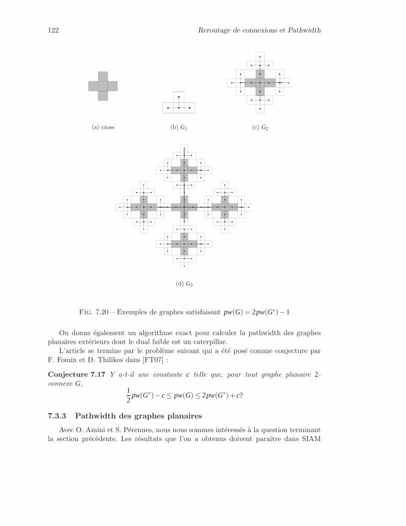
122 Reroutage de connexions et Pathwidth
(a) cross (b) G1 (c) G2
(d) G3
Fig. 7.20 – Exemples de graphes satisfaisant pw(G) = 2pw(G∗)−1
On donne également un algorithme exact pour calculer la pathwidth des graphesplanaires extérieurs dont le dual faible est un caterpillar.
L’article se termine par le problème suivant qui a été posé comme conjecture parF. Fomin et D. Thilikos dans [FT07] :
Conjecture 7.17 Y a-t-il une constante c telle que, pour tout graphe planaire 2-connexe G,
12
pw(G∗)−c≤ pw(G) ≤ 2pw(G∗)+c?
7.3.3 Pathwidth des graphes planaires
Avec O. Amini et S. Pérennes, nous nous sommes intéressés à la question terminantla section précédente. Les résultats que l’on a obtenus doivent paraître dans SIAM

Contributions 123
Journal of Discrete Maths [AHP] et je les présente ici. L’article figure dans l’Annexe E.3.Dans [FT07], les auteurs prouvent une version plus faible de la Conjecture 7.17. Ils
montrent qu’elle est vraie si l’on remplace les facteurs 1/2 et 2 respectivement par 1/6et 6. Dans [AHP] nous montrons qu’elle est vraie avec les facteurs 1/3 et 3 et qu’elleest également vraie si on se restreint aux graphes planaires quatre connexes.
Théorème 7.18 Pour tout graphe planaire 3-connexe G, on a 13 pw(G∗)−2≤ pw(G)≤
3pw(G∗)+2.
Théorème 7.19 Si G est un graphe planaire ayant un chemin Hamiltonien, alors12 pw(G)−1≤ pw(G∗) ≤ 2pw(G)+1. En particulier cela est vrai si G est 4-connexe.
Pour prouver ce théorème nous proposons, comme pour le Théorème 7.16, un al-gorithme qui transforme une décomposition en chemins du dual d’un graphe planaireen une décomposition en chemins du graphe lui même sans en faire plus que tripler lataille. La technique que l’on propose ne permet malheureusement pas de résoudre laConjecture 7.17 car il existe des graphes 3-connexes pour lesquels la taille de la décom-position en chemins obtenue par notre algorithme est le triple de la taille de celle deleur dual. Ce théorème englobe presque le Théorème 7.16.
Enfin, d’après une remarque de D. Coudert, un énoncé plus fort proposé dans [FT07]est faux :
Question 7.20 [FT07] Il existe une constante c telle que pour tout graphe planaire2-connexe G de treewidth au moins m, on a pw(G∗) ≤ m
m−1 pw(G)+c.
En effet, si on modifie légèrement la famille de graphes (illustrée par les Figures7.20(b) à 7.20(d)) de la section précédente en collant sur une face du graphe Gi unegrille i × i (cf Figures 7.21(a) et 7.21(b)) sa pathwidth ne change pas alors que satreewidth passe de 2 à i.
7.3.4 A propos de l’indice d’échappement arête connexe d’un arbre
7.3.4.1 Arbres pondérés et arbres de cliques
D’après un résultat de H. Bodlaender et T. Kloks, on sait que trouver la pathwidthd’un graphe de treewidth borné est polynomial [BK96] (le degré du polynôme dépendde la borne sur la treewidth). Cet algorithme a surtout un intérêt théorique dans lamesure où sa complexité est très élevée. Dans le cas des graphes planaires extérieurs,elle est supérieure à n11, alors que la treewidth vaut 2.
Si un tel résultat est vrai pour l’indice d’échappement arête connexe d’un graphe,calculer l’indice d’échappement arête connexe d’un arbre pondéré serait également po-lynomial en la somme des poids. En effet, on peut transformer un arbre pondéré en unarbre de cliques ayant le même indice d’échappement arête connexe.
Pour cela il faut d’abord remarquer que si un sommet a un poids inférieur au poidsd’une des arêtes qui lui sont incidentes, on peut augmenter son poids sans augmenterl’indice d’échappement arête connexe.

124 Reroutage de connexions et Pathwidth
(a) G2 modifié (b) G3 modifié
Fig. 7.21 – Les deux premiers exemples modifiés contredisant la Conjecture 7.20
Ensuite, on peut transformer un arbre pondéré (T,w) en un arbre de cliques commesuit : chaque sommet v est remplacé par une clique avec des arêtes doubles Cu dontla taille est le poids du dit sommet v moins un : w(v)− 1 (un sommet de poids 2est remplacé par un sommet avec une boucle). Le poids d’une arête uv est l’arêteconnectivité entre les deux cliques Cu et Cv remplaçant les sommets u et v. Si un sommetu est relié à deux sommets v1 et v2, la transformation est faite de telle sorte à maximiserΓ(Cv1)∩Cu∩Γ(Cv2). Cette transformation est illustrée par la Figure 7.22.
1
22
6
3
22
2
6
3
4
4
4
4
3
4
445
Fig. 7.22 – D’un arbre pondéré à un arbre de cliques.
Remarque 7.21 Le rôle des arêtes doubles dans une clique de taille k−1 est de forcerl’utilisation de k agents pour la nettoyer.
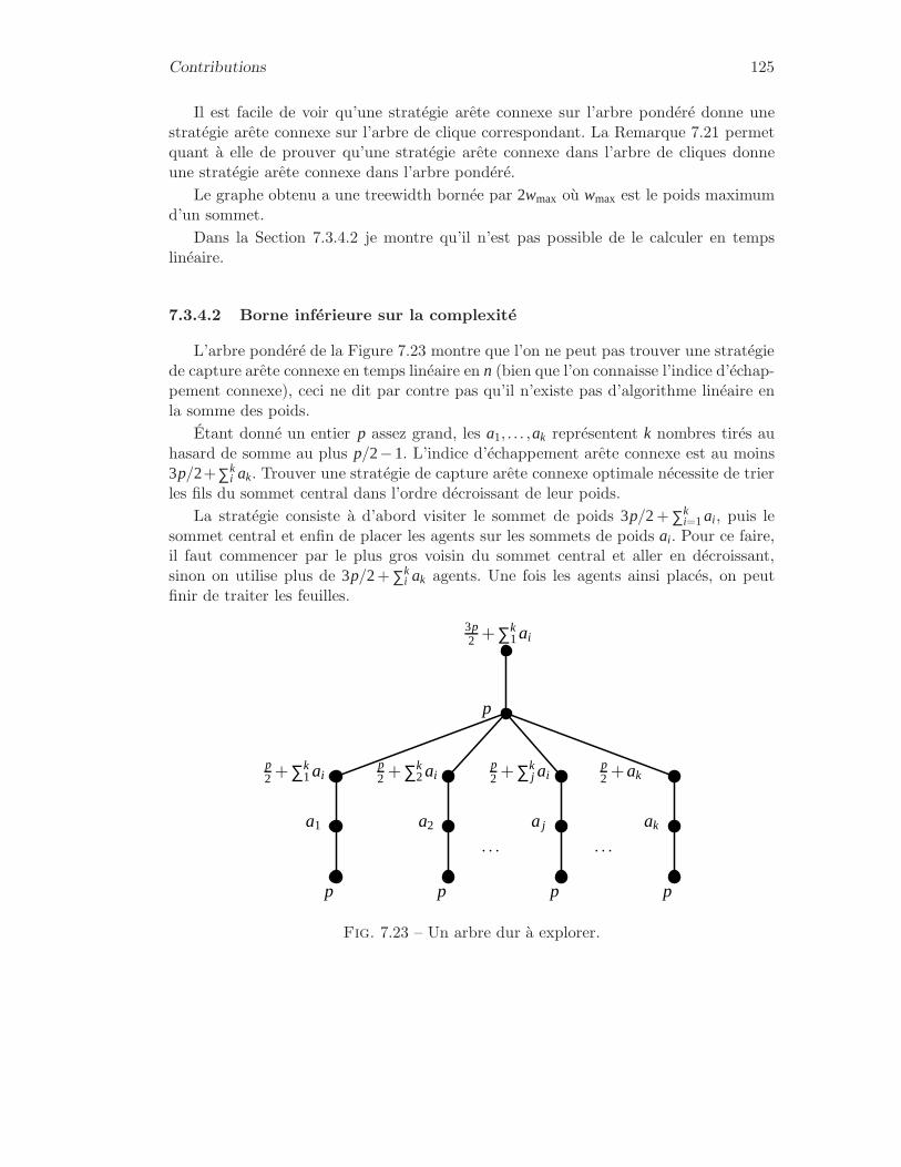
Contributions 125
Il est facile de voir qu’une stratégie arête connexe sur l’arbre pondéré donne unestratégie arête connexe sur l’arbre de clique correspondant. La Remarque 7.21 permetquant à elle de prouver qu’une stratégie arête connexe dans l’arbre de cliques donneune stratégie arête connexe dans l’arbre pondéré.
Le graphe obtenu a une treewidth bornée par 2wmax où wmax est le poids maximumd’un sommet.
Dans la Section 7.3.4.2 je montre qu’il n’est pas possible de le calculer en tempslinéaire.
7.3.4.2 Borne inférieure sur la complexité
L’arbre pondéré de la Figure 7.23 montre que l’on ne peut pas trouver une stratégiede capture arête connexe en temps linéaire en n (bien que l’on connaisse l’indice d’échap-pement connexe), ceci ne dit par contre pas qu’il n’existe pas d’algorithme linéaire enla somme des poids.
Étant donné un entier p assez grand, les a1, . . . ,ak représentent k nombres tirés auhasard de somme au plus p/2−1. L’indice d’échappement arête connexe est au moins3p/2+∑k
i ak. Trouver une stratégie de capture arête connexe optimale nécessite de trierles fils du sommet central dans l’ordre décroissant de leur poids.
La stratégie consiste à d’abord visiter le sommet de poids 3p/2+ ∑ki=1ai , puis le
sommet central et enfin de placer les agents sur les sommets de poids ai . Pour ce faire,il faut commencer par le plus gros voisin du sommet central et aller en décroissant,sinon on utilise plus de 3p/2+ ∑k
i ak agents. Une fois les agents ainsi placés, on peutfinir de traiter les feuilles.
p
p
a2
p
aj
p
ak
p
a1
p2 +∑k
1aip2 +∑k
2aip2 +∑k
j aip2 +ak
3p2 +∑k
1ai
. . .. . .
Fig. 7.23 – Un arbre dur à explorer.
126 Reroutage de connexions et Pathwidth
7.3.4.3 Version dynamique de l’indice d’échappement arête connexe nonpondéré
Dans [BFFS02], L. Barrière, P. Flocchini, P. Fraigniaud, N. Santoro définissent uneversion dynamique de l’indice d’échappement arête connexe et demandent s’il existe unalgorithme polynomial pour le calculer dans les arbres. Dans cette section, je montreque leur algorithme peut être adapté pour le calculer, sa complexité devient alors :O(nlog(n)). L’indice d’échappement arête connexe dynamique (dynamic conti-guous search number) est le nombre minimal d’agents nécessaires pour capturer unfugitif tel qu’à chaque tour des agents, l’un d’eux peut effectuer l’une des deux actionssuivantes :
– se positionner sur un sommet s’il n’est pas déjà positionné sur un autre sommet– se déplacer d’un sommet vers un sommet adjacent
tout en respectant la contrainte que la zone sûre reste connexe.A son tour, le fugitif peut se déplacer n’importe où dans le graphe tant qu’il ne
passe pas par un sommet v sur lequel est positionné au moins autant d’agents qu’il y ade sommets contaminés adjacents à v.
Dans ce cadre là, on peut montrer le lemme suivant :
Lemme 7.22 Étant donné un arbre T de racine y, si y1, . . . ,yp sont les fils de y telsque cs(Tyi ) ≥ cs(Tyi+1) pour 1≤ i < p, alors cs(T) = maxi(cs(Tyi )+ i −1).
Preuve. Comme on est dans le cas non pondéré, une stratégie qui traite partiellementun sous-arbre Tyi avant de traiter un autre sous-arbre Tyj peut être transformée en unestratégie utilisant autant d’agents et qui traite complètement Tyi avant de commencerà traiter Tyj . Il est alors clair qu’une stratégie va utiliser au moins maxi(cs(Tyi )+ i −1)agents et qu’une stratégie qui traite les sous arbres dans l’ordre Typ à Ty1 utilise cenombre d’agents.
Théorème 7.23 L’indice d’échappement arête connexe dynamique d’un arbre T peutêtre calculé de manière distribuée par un algorithme de complexité O(nlog(n)).
Dans l’algorithme proposé dans [BFFS02], remplacer l’utilisation du Lemme 7.9 parl’utilisation du Lemme 7.22 nécessite de trier les voisins de chaque sommet au lieu desélectionner les deux sommets qui sont racines des sous arbres ayant le plus grand indiced’échappement arête connexe. A chaque sommet v, le nombre d’opérations effectuéesest alors d(v) log(d(v)) au lieu de 2d(v). La complexité globale de l’algorithme est doncbien O(nlog(n)) comme annoncé.
7.4 Conclusion et Perspectives
Dans ce chapitre, je me suis intéressé au problème du reroutage, qui est nécessairedans les réseaux WDM dynamiques. Ce problème peut être modélisé par un problèmede traitement des sommets d’un graphe orienté des conflits. J’ai montré les liens entre
Conclusion et Perspectives 127
ce problème et divers problèmes dont le calcul de la pathwidth. Ensuite j’ai expli-qué le fonctionnement d’un algorithme permettant de calculer le process number d’unarbre. Dans la section suivante, j’ai présenté de nouveaux résultats sur les liens entrela pathwidth d’un graphe planaire extérieur et celle de son dual ainsi que sur les liensentre la pathwidth d’un graphe planaire et celle de son dual. Dans la dernière section,je présente une borne inférieure sur la complexité d’un algorithme calculant l’indiced’échappement arête connexe. Je présente également un lemme permettant d’adapterun algorithme qui calcule l’indice d’échappement arête connexe pour calculer l’indiced’échappement arête connexe dynamique.
Il reste de nombreuses questions ouvertes. Par exemple, la conjecture sur les liensentre la pathwidth d’un graphe planaire et celle de son dual n’est pas encore complè-tement résolue. Il n’existe toujours pas d’algorithme efficace permettant le calcul de lapathwidth d’un graphe planaire extérieur. De manière plus générale, il serait intéressantde pouvoir calculer ou tout du moins approximer de manière efficace le process num-ber des graphes de conflits apparaissant lors des reroutages de connexions. Pour citerun dernier problème, les liens entre les complexités du calcul de différents paramètresrestent encore flous.

128 Reroutage de connexions et Pathwidth

Chapitre 8
Conclusion
Comprendre et développer des outils combinatoires et algorithmiques pour la concep-tion de réseau et leur administration a été le sujet essentiel de ma thèse. J’ai utilisé desconcepts généraux permettant de résoudre divers problèmes apparaissant tout le longdu cycle de vie des réseaux. Les outils que j’ai utilisés m’ont permis d’avoir des ap-proches différentes et complémentaires. Mon travail n’est pas spécifique à un seul typede réseaux, au contraire j’en ai considéré plusieurs types dont des réseaux optiquesde cœur ou d’accès, des réseaux d’antennes, des réseaux d’accès WiFi, des réseaux enforme de grilles, ou bien encore des réseaux embarqués.
La diversité des réseaux jointe à celle des outils a permis de dégager plusieursproblématiques et d’en traiter un certain nombre. De nombreux problèmes permettantdes avancées dans les problématiques que j’ai dégagées peuvent être étudiées à la suitede cette thèse. Je résume ci-dessous mes contributions et quelque questions ouvertes.
– Concernant les réseaux embarqués, le problème, posé par Alcatel Space Industrie,est de concevoir des réseaux capables de router p signaux arrivant par p entréesparmi p+λ vers p des p+k sorties. J’ai présenté des techniques permettant d’ob-tenir des bornes inférieures sur la taille de ces réseaux ainsi que des constructions.Les constructions sont pour la plupart asymptotiquement optimales quand les va-leurs de λ et k sont bornées par log(n)/15. J’ai également présenté des résultatssur un nouveau paramètre, qui est une variante de l’expansion, l’α-robustessepermettant de construire des réseaux pour de plus grandes valeurs de k et λ.
Q : L’étude de l’α-robustesse n’est pas terminée. Afin d’avoir des construction ex-plicites de réseaux, il est nécessaire d’avoir des constructions explicites de graphesayant une grande α-robustesse. De plus, nous avons vu que l’α-robustesse d’ungraphe à n sommets est au plus n
2 quand α > 45. Est il possible de généraliser ce
résultat et de donner une condition sur α assurant une α-robustesse d’au plusn/3 par exemple ?
– Pour le dimensionnement et l’exploitation des réseaux, je me suis ensuite intéresséau problème de routage. Ce problème est important lors de la conception desréseaux afin de dimensionner les liens au mieux, et lors de son exploitation. Dans
129
130 Conclusion
ce dernier cas, les solutions doivent pouvoir être calculées rapidement. Il existe denombreuses versions du problème de routage et autant de manières de l’aborder.J’ai eu trois approches différentes.
1. La première est la conception d’algorithmes, soit optimaux, soit d’approxi-mation. Cela a été le cas pour les problèmes de routage de paquets dans lesréseaux en forme de grille, pour lesquels j’ai présenté des algorithmes opti-maux dans le cas du routage r-central, de la permutation et du (ℓ,ℓ)-routage,et un algorithme d’approximation pour le (ℓ,k)-routage. J’ai aussi conçu desalgorithmes d’approximation pour le problème de routage dans les réseauxd’antennes, problème modélisé par la coloration k-impropre de graphes pon-dérés. Les coefficients des algorithmes d’approximation sont, pour k de un àcinq, 25
13, 127 , 18
13, 8063 et 49
43. J’ai également étudié et montré que le problèmed’ordonnancement de requêtes à taux constant est NP-dur dans les réseauxd’accès WiFi.
Q : Concernant les algorithmes d’approximation pour le routage dans les réseauxd’antennes, problème modélisé par la coloration k-impropre, il serait intéres-sant de savoir si des algorithmes ayant de meilleurs rapports d’approximationexistent, et également quel est le meilleur rapport d’approximation que l’onpeut garantir en temps polynomial.
Q : Pour le problème du routage des requêtes à taux constant, modélisé par lacoloration proportionnelle, il n’existe pas encore d’algorithmes d’approxi-mation. Il serait donc intéressant d’en développer ou de trouver d’autresfamilles de graphes pondérés pour lesquelles calculer l’indice chromatiqueproportionnel est polynomial.
2. La deuxième approche a été de comparer deux modes de routages différents :le routage unicast et le routage multicast. Pour cela j’ai étudié un problèmede coloration -le directed star colouring- sur lequel j’ai fait de nombreusesavancées ; il est entre autre prouvé que dst(D) ≤ 2∆−(D)+1 et que dst(D) ≤2max(∆+(D),∆−(D)). Ce problème permet de dire que dans le cas d’un réseauoptique équipé de splitters, si le routage est de profondeur bornée et que lenombre de feuilles de chaque arbre de routage est borné par une constantefois la charge maximale du réseau ℓ, il suffit de ℓ+O(log(ℓ)) longueurs d’ondepour le réaliser alors que si le réseau n’est pas équipé de splitters, il peutfalloir jusqu’à (∆ + 1)ℓ longueurs d’onde où ∆ est le degré maximum duréseau.
Q : Les travaux sur le directed star colouring peuvent être poursuivis. En effetil reste plusieurs conjectures à résoudre. En particulier, est-il vrai que pourtout graphe orienté D, on a dst(D) ≤ 2∆−(D) ?
3. Enfin, la troisième approche du problème de routage a été de concevoir desmodèles mathématiques pour le résoudre à l’aide d’un solveur. J’ai utilisé
Conclusion 131
cette approche pour le problème de routage de multicasts dans les réseauxoptiques de cœur et d’accès, pour le problème de routage d’unicasts dans lesréseaux avec groupes de risques partagés, et pour le problème de protectionpar segments.
Q : Quant aux problèmes de routage pour lesquels j’ai conçu des modèles mathé-matiques dont je vais implémenter les formulations qui ne l’ont pas encoreété, ils sont une première étape pour l’étude de problèmes plus complexesdont le routage de multicast dans les réseaux ayant des groupes de risqueset la protection dans ces mêmes réseaux, tant des unicasts que des multi-casts. Pour ces problèmes, il est difficile de concevoir des algorithmes d’ap-proximation pertinents car les requêtes que l’on considère et les réseaux sontquelconques. Il serait intéressant de savoir s’il existe une structure type dansla topologie des requêtes et dans l’affirmative de l’étudier et d’en proposerun modèle pour pouvoir concevoir des algorithmes d’approximation.
– Pour un réseau dont les requêtes évoluent dynamiquement, plutôt que de recal-culer à chaque changement un nouveau routage, il est plus intéressant de se basersur le routage existant et de le faire évoluer. C’est ce problème -passer d’un rou-tage à un autre- que j’ai étudié dans le Chapitre 7. Ce problème est associé àun paramètre : le process number. J’ai présenté un algorithme qui calcule le pro-cess number des arbres. Je présente ensuite un algorithme d’approximation pourles graphes planaires extérieurs qui a un facteur d’approximation de deux. Leprocess number étant fortement lié à la pathwidth, j’ai également étudié ce para-mètre et fait plusieurs avancées sur des conjectures. Il est entre autre prouvé quetout graphe planaire extérieur G biconnexe vérifie pw(G∗)≤ pw(G)≤ 2pw(G∗)−1.Pour les graphes planaires, il est prouvé que tout graphe planaire trois connexeG vérifie pw(G∗)/3−2≤ pw(G) ≤ 3pw(G∗)+2 et que les graphes planaire quatreconnexe G vérifient pw(G∗)/2−1≤ pw(G) ≤ 2pw(G∗)+1.
Q : Concernant le process number et la pathwidth, il reste à trouver un algorithmepermettant de calculer ces paramètres sur les graphes planaires extérieurs etd’autre classes de graphes. Il serait également intéressant de savoir si pour tousles graphes planaires G, on a pw(G∗)/2−1≤ pw(G)≤ 2pw(G∗)+1. J’ai égalementprésenté plusieurs paramètres -pathwidth, process number, edge search number,contiguous search number- dont on ne sait pas si ils sont équivalents. Est-il pos-sible, connaissant l’un d’eux, de calculer les autres en temps polynomial ?
– Enfin, j’ai étudié un problème théorique permettant de mieux comprendre lastructure des graphes orientés. J’ai présenté une nouvelle caractéristique, appeléef -mixing. Il est prouvé que la plus grande valeur de f telle que tout grapheorienté f -mixing contient un circuit orienté de longueur quatre est C1e2/n2 pourune petite constante C1. Il est également montré que pour tout graphe orienté Hbiparti, il existe une constante C′
1 telle que tout graphe orienté C′1-mixing ayant
suffisamment d’arêtes contient H comme sous-graphe.Q : À propos des graphes orientés f -mixing, il reste beaucoup de questions ouvertes.

132 Conclusion
La valeur de mex(n,e,H) n’est connue que quand e est de l’ordre de n2 ou quandH est une orientation du cycle de longueur quatre. Tous les autres cas restent àrésoudre. Une autre question importante est de trouver la complexité du problèmede calculer, dans un graphe orienté, deux ensembles A et B tels qu’il n’y a pasd’arcs de B vers A et que le nombre d’arcs de A vers B soit maximum. Tout ceque l’on sait est que ce problème est NP-dur dans le cas des graphes orientés.

Annexe A
Conception de réseaux tolérantsaux pannes
A.1 Minimal Selectors and Fault Tolerant Networks
Article accepté pour publication dans Networks.
133

Minimal Selectors and Fault Tolerant Networks∗
Omid Amini1,2 Frederic Giroire 2,3 Florian Huc 2
Stephane Perennes 2
Abstract
In this paper we study a combinatorial optimization problem arising fromon-board networks in satellites. In these kinds of networks the entering signals(inputs) should be routed to amplifiers (outputs). The connections are madevia expensive switches with four available links. The paths connecting inputsto outputs should be link-disjoint. More formally, we call a (p, λ, k)−networkan undirected graph with p + λ inputs, p + k outputs and internal vertices ofdegree four. A (p, λ, k)−network is valid if it is tolerant to a restricted numberof faults in the network, i.e., if, for any choice of at most λ faulty inputs andk faulty outputs, there exist p edge-disjoint paths from the remaining inputsto the remaining outputs.
Our optimization problem consists of determining N(p, λ, k), the minimumnumber of vertices in a valid (p, λ, k)−network. We present validity certifi-cates and a quasi-partitioning technique from which we derive lower boundsfor N(p, λ, k). We also provide constructions, and hence upper bounds, basedon expanders. The problem is shown to be sensitive to the order of λ and k.For instance, when λ and k are small compared to p, the question reduces tothe avoidance of some forbidden local configurations. For larger values of λ
and k, the problem is to find graphs with a good expansion property for smallsets. This leads us to introduce a new parameter called α-robustness. We useα-robustness to generalize our constructions to higher order values of k andλ. In many cases, we provide asymptotically tight bounds for N(p, λ, k).
Keywords: Fault Tolerant Networks, Switching Networks, Network Design,Concentrators, Routing, Connectivity, Disjoint paths, Expanders.
1 Introduction
Motivation. One of the most fundamental problems in many applications ofcomputer science and graph theory is the design of efficient networks. Efficientcan have several meanings depending on the context. Properties such as highconnectivity, fault tolerance and being algorithmically simple are at the heart ofsuch concerns. In this paper we study a combinatorial optimization problem of thiskind. The problem, originally posed by Alcatel Space Industry, comes from
∗This work has been partially supported by European project IST FET AEOLUS.1Ecole Polytechnique, Palaiseau, FRANCE, [email protected], joint project- INRIA/CNRS-I3S/UNSA- 2004, route des Lucioles - Sophia-
Antipolis, FRANCE, [email protected] work was done while in the Algorithms project, INRIA Rocquencourt, F-78153 Le Ches-
nay, France.
1

1 INTRODUCTION 2
the design of efficient on-board networks in satellites (also called Traveling WaveTube Amplifiers). The satellites under consideration are used for TV and videotransmission (like the Eutelsat or Astra series) as well as for private applications.Signals incoming to a telecommunication satellite through ports have to be routedthrough an on-board network to amplifiers. A first constraint is that the networkshould be built with switches having four links. But other constraints appear. Onthe one hand, the amplifiers may fail during the satellite’s life time and can not berepaired. On the other hand, as the satellite is rotating, not all the ports are welloriented and hence available. So more amplifiers and ports are needed than thenumber of signals which have to be routed. Notice that in this context, contrary tothe classical networks, we do not consider link and switch failure. As a matter of factthe links are just big tubes and the switches are very reliable rotating mechanicalsystems.One can easily construct a network fulfilling these constraints by using a permuta-tion network or two concentrators of any fixed degree. However, to decrease launchcosts, it is crucial to minimize the network physical weight, i.e., to minimize thenumber of switches. Switches are also expensive to build, so it is worth saving evenone. Space industries are interested in designing such networks for specific valuesof the parameters, however the general theory is of interest by itself. Also, due tothe increasing launch capacities and the decreasing switch sizes, larger networkswill be used in a near future.
Problem. We consider here networks, connecting a set of inputs to a set of outputs.A network can be seen as a graph with a set of inputs and outputs. The verticesof this graph represent the switches. We define a (p, λ, k)−network as a networkwith p + λ inputs and p + k outputs. A (p, λ, k)−network is said to be valid if itcan tolerate up to λ faults in inputs and up to k faults in outputs. More formallyfor any choice of p inputs and p outputs, there exist p edge-disjoint paths linkingall the chosen inputs to all the chosen outputs. By symmetry, we may assume inthe following that k ≥ λ and we denote the total number of outputs by n := p + k.Fig 1 gives an example of a (12,4,4) valid network with 20 switches (the inputsare represented with arrows, the outputs with squares and the switches with blackvertices).
Note that finding minimal networks is a challenging problem and even testingthe validity of a given network is hard (see related work). We study the case wherethe switches of the network have degree four (although the theory can be generalizedto any degree) which is of primary interest for the applications. The problem is tofind N(p, λ, k), the minimum number of switches in a valid (p, λ, k)−network, andto give constructions of such networks.
Related Work. This study of a new kind of networks should be considered in thespirit of the well studied theory of superconcentrators. A (p+k, p)-concentrator [31]is a directed acyclic graph G = (V, E) with p + k designated input vertices and pdesignated output vertices (k ≥ 0), such that for each subset of p input vertices,there exist p edge-disjoint (or, depending on the context, vertex-disjoint) pathsfrom the input vertices to the output vertices. A selector, first introduced in [9],is a (p, 0, k)-network (λ = 0). A general theory of selectors can be found in [12],where several results are obtained for small values of k. A selector can be seen asan undirected version of a (p + k, p)-concentrator by changing the role of inputsand outputs (and by adding the degree condition). An n-superconcentrator [28]

1 INTRODUCTION 3
is a directed acyclic graph G = (V, E) with n designated input vertices and ndesignated output vertices such that, for any set S of p ≤ n inputs and any set T ofp outputs, there exist p edge-disjoint (or, vertex-disjoint depending on the context)paths connecting S to T . There is a vast theory of superconcentrators (see theseminal work of Pippenger [28] for an introduction, [2, 3, 5, 30] for constructions,and [14] for complexity issues).
In this way, (p, λ, k)-networks generalize the concept of selectors as supercon-centrators generalize concentrators. It is also clear that taking a superconcentrator(resp. (p + k, p)−concentrator) and forgetting the orientations provides a valid(p, λ, k)-network (resp. selector) for every value of k = λ (resp. any k and λ = 0),once the degree condition is respected. So one can try to use superconcentratorsto construct efficient on-board satellite networks, but, not surprisingly, this doesnot give minimal networks in general. The major difference between the supercon-centrators and the general valid networks, beside the degree condition, is that in avalid network the number of inputs and outputs that may become out of service isbounded (in our case, given a failure probability, no more than k failures will occurduring the satellite lifetime). Finding a minimum network (a superconcentrator oflow density or having a minimum number of vertices) is a challenging problem andis an active area of research. From the algorithmic point of view, one can showthat the problem of testing if a graph is a (p + k, p)-concentrator or a supercon-centrator is coNP-complete. In fact, this is coNP-complete even when restrictedto the important special case of graphs of size linear in the number of inputs (see[14]). By the same arguments one can prove that the problem of deciding if a given(p, λ, k)-network is valid or not is coNP-complete.
In [12] the authors consider a variant of selectors where some signals have pri-ority and should be sent to amplifiers offering the best quality of service. In [8]the authors study the case where all the amplifiers are different and where a giveninput has to be sent to a dedicated output. This problem is related to permutationnetworks.
In [11, 21], the authors present exact values of N(p, λ, k) for small values of k andλ and arbitrary values of p. For instance N(p, 2, 1) = N(p, 1, 2) = N(p, 2, 2) = p+2and also for k ∈ 3, 4 and 0 < λ ≤ 4, N(p, λ, k) = ⌈ 5n
4 ⌉.
Figure 1: A valid (12,4,4)-network with the minimum number of switches. Switches,vertices of the corresponding graph, are represented by •.
2 PRELIMINARIES 4
Results. In this paper we are primarily interested in large networks, i.e., wheren = p+k tends to infinity and also k is large enough. We present several upper andlower bounds for the minimum number of switches in a valid (p, λ, k)−network. Inmany cases these bounds are asymptotically tight. Since forgetting the orientationof superconcentrators provides valid (p, λ, k)−networks, these results also providelower bounds on the size of a superconcentrator. To obtain the lower bounds wepresent a new technique, quasi-partitioning. We give here the very first applica-tions of this lemma, but we think it may have several applications in other relatedproblems (for example bisection-width, see [24]).
To obtain upper bounds we propose several constructions. The constructionof optimal valid networks will heavily rely on expanders (see Section 4.1). Usingthese, we are able to construct, for a special class of networks called simplifiednetworks, networks with 2n switches as soon as n is large enough and k ≤ c1 log nfor some constant c1 (Section 4.3). In Section 6 we also give a lower bound of order2n(1− ǫ(k)) where ǫ(k) tends to zero when k tends to infinity (but we do not needk ≤ c1 log n). Thus for simplified networks the problem is asymptotically solved fork ≤ c1 log n. For general networks, using bipartite expanders, we obtain an upperbound of n + 3
4n when k ≤ c2 log n for some constant c2. The lower bound weobtain is (n + 2
3n)(1 − ǫ(λ, k)), and we conjecture that n + 34n should be the right
value. We also give a construction of selectors (case λ = 0) of size n + n2 , in which
case we get also a tight lower bound.To extend the results to larger values of k, we define a local expansion property
of graphs that we call α−robustness (see [4, 16] for some related notions). Intu-itively, the α−robustness of a graph G is a local version of the expansion factor.It is the maximum integer rα such that for small subsets the expansion factor is αbut for larger subsets, the minimum number of outgoing edges is required to be atleast rα. In our constructions, we only need our graph to be an expander for smallsubsets, but for larger subsets all we need is a minimum constant edge-connectivityto the rest of the graph. This notion is also interesting in its own right, and con-tains several expansion-invariants such as bisection-width and Cheeger’s constantas special cases (see [18]). As random graphs are very good expanders, we study theα−robustness of random graphs. In this way we generalize Bollobas’ result on theexpansion factor of random 4-regular graphs (see [15]) to obtain related results forα−robustness of random 4-regular graphs. As far as we know it is the first time inthe literature that this new concept of local expanders is defined and investigated.Using this we present a construction of valid (p, λ, k)−networks with 3n switchesfor λ ≤ k ≤ n
7 .
2 Preliminaries
In this section, we define more formally the design problem and introduce notationused throughout the paper. We state a cut criterion (Proposition 1): this criterionis fundamental because it characterizes the validity of (p, λ, k)−networks. It is ex-tensively used to prove that networks are valid —in particular for the networks ofSection 4. In Section 6 we also use the cut criterion to detect forbidden patternsleading to lower bounds for the number of switches of valid networks. Proofs oflower and upper bounds are simplified by the use of the last notion introduced here,the associated graph of a network (see Section 4.2 and Section 6.1).

2 PRELIMINARIES 5
Notation. Given a function f , we define f(A) :=∑
a∈A f(a) for any finite set A.For a subset W of vertices of a graph G = (V, E), let us denote by ∆(W ) the set ofedges connecting W and W = V \W and by Γ(W ) the set of vertices of W adjacentto a vertex of W . If a set is denoted by an upper case letter, the correspondinglower case letter denotes its cardinality (for example δ(W ) = |∆(W )|).
(p, λ, k)−Networks and Valid (p, λ, k)−Networks. A (p, λ, k)−network is atriple N = (V, E), i, o where (V, E) is a graph and i, o are non-negative integerfunctions defined on V called input and output functions, such that for any v ∈ V ,i(v) + o(v) + deg(v) = 4. The total number of inputs is i(V ) = Σv∈V i(v) = p + λ,and the total number of outputs is o(V ) = Σv∈V o(v) = p+k. We can see a networkas a graph where all vertices but the leaves have degree four, and in which inputsand outputs are leaves. A non-faulty output function is a function o′ defined on Vsuch that o′(v) ≤ o(v) for any v ∈ V and o′(V ) = p. A used input function is afunction i′ defined on V such that i′(v) ≤ i(v) for any v ∈ V and i′(V ) = p. A(p, λ, k)-network is said valid if for any non-faulty output function o′ and any usedinput function i′, there are p edge-disjoint paths in G such that each vertex v ∈ Vis the initial vertex of i′(v) paths and the terminal vertex of o′(v) paths.
Design Problem and Simplified Design Problem. Let N(p, λ, k) denote theminimum number of switches of a valid (p, λ, k)-network. The Design Problem con-sists of determining N(p, λ, k) and constructing a minimum (p, λ, k)-network, or atleast a valid (p, λ, k)-network with a number of switches close to the optimal value.We introduce a variation of the problem, the Simplified Design Problem, which is tofind minimum networks having p + λ switches with one input and one output andk − λ switches with only one output. Networks of this kind are especially good forpractical applications, as they simplify the routing process, minimize path lengthsand lower interferences between signals.
Excess, Validity and Cut Criterion. To verify if a network is valid, insteadof solving a flow/supply problem for each possible configuration of output failuresand of used inputs, it is sufficient to look at an invariant measure of subsets of thenetwork, the excess, as expressed in the following proposition.
Proposition 1 (Cut Criterion) A (p, λ, k)−network is valid if and only if, forany subset of vertices W ⊂ V the excess of W , defined by
ε(W ) := δ(W ) + o(W ) − min(k, o(W )) − min(i(W ), p),
satisfies ε(W ) ≥ 0.
The intuition is that the signals arriving in W (in number at most min(i(W ), p))should be routed either to the valid outputs of W (in number at least o(W ) −min(k, o(W ))) or to the links going outside (in number δ(W )). The omitted formalproof reduces to a supply/demand flow problem. Note that, for the cut criterion, itis sufficient to consider only connected subsets W with connected complement W(this comes from the submodularity of ε).
Associated Graph. Vertices x ∈ V of degree two with i(x) = o(x) = 1 play animportant role. We call them doublons. A switch that is not a doublon is called an

3 SUMMARY OF MAIN RESULTS 6
R-switch. Remark that for k ≥ 3 no paths has three or more consecutive doublons.Indeed if we consider the set W consisting of these doublons we have δ(W ) = 2 ando(W ) = i(W ) ≥ 3. The cut criterion would give a contradiction.
Let N be a (p, λ, k)−network. We build a graph R associated with N . Itsvertices are the R-switches of N . Consequently the edges of R are of three kinds,respectively E0, E1 and E2: the edges of N between two R−switches, the edgescorresponding in N to a path of length two with a doublon in the middle and thosecorresponding to a path of length three with two doublons in the middle.
3 Summary of Main Results
The aim of this short section is to provide an overview of the results obtained inthe upcoming sections.
The design problem is treated in Sections 4 and 5. For relatively small valuesof k and λ, based on expanders, we provide construction of valid networks forthe general design problem, the design problem when λ = 0 (selectors) and thesimplified design problem. More precisely, we prove the following theorems:
Theorem 2 of Section 4 (General Design Problem). Let n = p + k, k ≤ 115 log n,
for n large enough, we have: N(p, λ, k) ≤ n + 34n
Theorem 3 of Section 4 (Selectors, λ = 0). Let n = p + k, k ≤ 148 log2 n, for n
large enough, we have:
N(p, 0, k) ≤ n +n
2.
Theorem 1 of Section 4 (Simplified Design Problem). Let n = p+k, k ≤ 16 log n,
for n large enough, we have: N(p, λ, k) ≤ 2n.
In Section 5, we provide a general framework to extend the above mentionedresults to larger values of λ and k. We define a new parameter, which we callrobustness, which captures the local expansion property of a given graph. Westudy the robustness of random regular graphs and use these graphs for the designproblem. In particular, we prove
Theorem 4 of Section 5. Random 4-regular graphs have 1-robustness at leastn14 with high probability, i.e., with probability 1 −O( log n
n ).
Corollary 1 of Section 5. For k ≤ n7 , there exist (p, λ, k)−valid networks of size
3n (remember that n = p + k).
The lower bounds, confirming the tightness of the above results in many cases,are provided in Section 6. We first prove a technical quasi-partition lemma:
Lemma 4 of Section 6. Let q be a positive integer and let G be a connectedgraph of order at least q
3 . Then G admits a q-quasi-partition (for the definition seeSection 6).
Using this lemma, we prove the following general theorem:
Theorem 5. In a valid network N of size N , with k ≤ n2 , we have
4 UPPER BOUNDS: THE DESIGN PROBLEM 7
N ≥(
3
2n − (k − λ) − 4 − 12√
k
)(
1 − 9
2√
k+ O
(
1
k
))
+d
2
(
1 +9
2√
k+ O
(
1
k
))
.
where n = p + k and d is the number of doublons, i.e., switches with exactly oneinput and one output.
Corollaries of this theorem are
Theorem 8 of Section 6 (General case). When λ → ∞ and k → ∞, any validnetwork has size at least n+ 2
3n+O( n√λ). In particular, N(p, λ, k) ≥ n+ 2
3n+O( n√λ).
Theorem 6 of Section 6 (Selectors). In a valid selector N of size N , when k → ∞with k ≤ n
2 , we have
N ≥ n +n
2+ O(
n√k
).
In other wordsN(p, 0, k) ≥ n +
n
2+ O(
n√k).
Theorem 7 of Section 6 (Simplified case). In the simplified case, when k →∞ with k ≤ n
2 , every valid network has size at least 2n + O( n√k), i.e., we have
N(p, λ, k) ≥ 2n + O( n√k) in the simplified case.
4 Upper Bounds: The Design Problem
In this section, we give constructions that rely heavily on expanders. We presenthere three constructions with 2n, n + 3
4n and n + n2 switches respectively for the
simplified design problem, the design problem (any λ) and for the design problemwhen λ = 0. All these constructions are valid for k ≤ c · log n (where c is a constantdepending only on the expansion factor of 3 and 4−regular graphs).
4.1 Expanders
An expander (see [26, 27] for surveys) is a highly connected sparse graph. Theyare used in various fields of computer science and mathematics. For example theyare valuable in constructions of error-correcting codes with efficient encoding anddecoding algorithms, derandomization of random algorithms, and embeddings offinite metric spaces. But they also have applications in areas directly related tothe subject of this paper as in the design of explicit superefficient networks and theexplicit construction of graphs with large girth (length of the smallest cycle). Wepresent here known results about expanders that are used in proofs of Sections 4.3,4.4 and 4.5. The formal definition of an expander is as follows: an (n, r, c)-E-expander is a finite r-regular graph G = (V, E) with n vertices such that for anyset A of vertices of G with |A| ≤ |V |/2 we have δ(A) ≥ c|A|. Well known examplesof expanders are Ramanujan graphs (for more on Ramanujan graphs see [25] andthe book [19]). Explicit constructions of Ramanujan graphs are known for r of theform r = q + 1, with q a prime power (in particular for r = 3 and r = 4, which are
4 UPPER BOUNDS: THE DESIGN PROBLEM 8
of special interest in our case). More precisely there exist explicit constructions ofan infinite family Gi = (Vi, Ei) of Ramanujan graphs such that |Vi| →
i→∞∞ with an
expansion factor c ≥ 1 − 4(r−1)r2 . It gives c ≥ 1
4 for 4−regular graphs and c ≥ 19 for
3-regular graphs. The girth of the graphs of this family satisfies: g(Gi) ≥ 23 logq |Vi|.
There also exists a family Hi = (Wi, Fi) of explicit bipartite Ramanujan graphs ofgirth g(Hi) ≥ 4
3 logq |Wi|. Probabilistic arguments show the existence of graphs, forany large order of networks (and not only for the specific values of both families),with the same properties of girth and even better expansion factor: for 4-regulargraphs, expanders with c ≥ 11
25 exist (see [15]).We also need a vertex-expansion version of expanders:
Definition 1 (V -Expander) An (n, r, d)-V -expander is a finite r-regular graph G =(V, E) with |V | = n (|V1| = |V2| = n in case of a bipartite graph and V = V1 ∪ V2)such that for any subset A of vertices (A ⊂ V1 when G is bipartite), the set ofneighbors of A, Γ(A) = v ∈ V |(v, u) ∈ E for some u ∈ V satisfies
|Γ(A)| ≥ |A| + d(1 − |A|/n)|A|.
4.2 Cut Criterion for the Associated Graph
To simplify the proofs of validity of Sections 4.3, 4.4 and 4.5, it is sometimesbetter to work directly on the associated graph R of the (p, λ, k)−network N =((V, E), i, o). More precisely, it means that, when applying the cut criterion on N ,it would be sufficient to consider only subsets of R.
We introduce another notion of excess, ε′, defined for all W ⊂ V as ε′(W ) :=δ(W ) + o(W ) − min(k, o(W )) − i(W ). Note that ε′(W ) ≤ ε(W ). Hence, if, for allW ⊂ V , ε′(W ) ≥ 0, the network is valid. But we have no more an equivalence.The good property of ε′ is that, if a switch x is a doublon, ε′(W ∪ x) ≤ ε′(W ).So it is enough to verify the cut criterion for subsets W of N consisting of a set ofR−switches plus all the doublons on the edges of type E1 and E2 incident to theR−switches.
4.3 Simplified Design Problem - Upper Bound 2n
In this subsection, we use the existence of expanders presented in Section 4.1 toconstruct valid (p, λ, k)−networks with 2n = 2(p + k) switches for large n andk ≤ c1 log n (c1 depending on the expansion factor of 4−regular expanders, c1 = 1
6when using explicit Ramanujan graphs). Furthermore we will show in Section 6 alower bound of the same order for the simplified design problem.
Theorem 1 Let n = p + k, k ≤ 16 log n, for n large enough, we have: N(p, λ, k) ≤
2n.
Proof The results on expanders presented in Section 4.1 state the existence of an(n, 4, c = 1
4 )−E-expander, G = (V, E), of girth g, g ≥ 23 log n. Let k ≤ c · g and
p = n − k. We claim that in a 4−regular graph there exists a family of vertex-disjoint cycles covering all vertices of G. For now, suppose this is true and call thisdisjoint union of cycles F . We add n new vertices on each edge of F by subdividing
4 UPPER BOUNDS: THE DESIGN PROBLEM 9
each edge of F into two edges. On each new vertex, we add an output and inputcreating a doublon. We now have a (p, k, k)−network N with 2n switches.
Let us prove that the constructed network is valid. We use the cut criterion onR, which, in that case, is exactly G. Notice first that the network is symmetricin inputs and outputs and that for any subset W ⊂ V of vertices, i(W ) = o(W ).Hence we have
ε′(W ) = δ(W ) − min(k, o(W )).
Furthermore, note that when a network is symmetric, it is sufficient to verify thecut criterion only for subsets W with |W | ≤ |V |/2.
- If |W | ≥ kc then, by the expansion property, there are at least k edges between
W and W and so ε′(W ) ≥ 0.
- Otherwise, if |W | < kc ≤ g, we have |W | < g and thus W is acyclic. There
are at most |W | − 1 edges inside W and, as G is 4-regular, we have δ(W ) ≥2|W |+2. Let eF (W ) be the number of edges of F incident to a vertex of W ; byconstruction o(W ) = eF (W ). As the cycles of F are disjoint, eF (W ) ≤ 2|W |.Hence δ(W ) ≥ eF (W ) = o(W ), that is ε′(W ) ≥ 0.
The (p, k, k)−network is valid. We can derive (p, λ, k)−networks for any λ ≤ k bydeleting k − λ inputs.
The only remaining point now is to prove the claim. We prove it for any 2r-regular graph. Let G = (V, E) be a 2r−regular graph. Since G is Eulerian, wecan give to G an orientation, such that each vertex has in-degree and out-degree r.Let D = (V, A) be the corresponding digraph. Now consider the following bipartitegraph: H = (V × 1 ∪ V × 2, E′) where E′ = ((x, 1), (y, 2))|(x, y) ∈ A. It isclear that H is a bipartite r-regular graph, and so it admits a perfect matching.Let F be the edges of G given by this perfect matching. It is easy to check thatF is a 2-regular graph covering all the vertices, i.e., F is a disjoint union of cyclescovering all the vertices.
4.4 General Design Problem - Upper Bound n + 34n
In this subsection, we construct general N(p, λ, k)−networks for large n, k ≤ c2 log n(where c2 depends on the expansion factor of 3−regular expanders). Theorem 2gives an n + 3
4n upper bound for such networks. Constructions are based on 3-regular bipartite expanders.
Definition 2 Two edges are at distance at least d if any path that contains bothof them is of length at least d + 2. A vertex is at distance at least d of an edge ifany path that contains both of them is of length at least d + 1.
Lemma 1 Let G be a 3−regular bipartite graph G = (V1 ∪ V2, E) of large girth(g = Θ(log |V1|)) which is a (2|V1|, 3, c)-E-expander and suppose 2k ≤ cg. Let F bea set of selected edges, such that any two edges of F are at distance at least 3. Thenetwork N obtained from G by adding a doublon on each edge of F , an input oneach vertex of V1 and an output on each vertex of V2 is a valid network.
4 UPPER BOUNDS: THE DESIGN PROBLEM 10
ProofWe use the cut criterion on the associated graph following Section 4.2. As
the construction is symmetric in inputs and outputs, it is sufficient to consider
connected subsets W ∈ V with |W | ≤ ⌈ |V |2 ⌉. The cut criterion is implied by
ε′(W ) = δ(W ) + o(W ) − min(o(W ), k) − i(W ) ≥ 0.
We now distinguish two cases for W . case 1: |W | ≤ 2kc ≤ g.
As o(W ) − min(o(W ), k) ≥ 0, we have
ε′(W ) ≥ δ(W ) − i(W ).
Hence it is sufficient to prove δ(W ) ≥ i(W ). As |W | ≤ g, there are no cyclesinside W and therefore there are |W | − 1 edges inside; G is 3−regular, soδ(W ) = |W |+2. Furthermore, i(W ) = |V1∩W |+d, so we have to prove that|V2 ∩ W | + 2 ≥ d.
Consider a doublon D incident to W and its associated edge e(D) = v1(D), v2(D)with v1(D) ∈ V1 and v2(D) ∈ V2. If v2(D) ∈ W , associate D with v2(D). Ifv2(D) /∈ W , then v1(D) ∈ W . Associate to D a neighboor of v1(D) ∈ W . Asthe distance of two edges of F is at least 3, different doublons have differentassociate vertices in V2 ∩ W . So |V2 ∩ W | ≥ d. case 2: |W | ≥ 2k
c . By definition of ε′ we have
ε′ ≥ δ(W ) + o(W ) − k − i(W ).
– If i(W ) − o(W ) ≤ k, by the expansion property, we have δ(W ) ≥ 2k ≥i(W ) − o(W ) + k.
– If i(W ) − o(W ) ≥ k, since the graph is bipartite, there are at least3(i(W )−o(W )) outgoing edges. So ε′(W ) ≥ 2(i(W )−o(W ))−k ≥ k > 0.
Theorem 2 (Construction) Let n = p + k, k ≤ 115 log n, for n large enough, we
have: N(p, λ, k) ≤ n + 34n.
Proof Take H = (A, B, E), a bipartite (2|A|, 4, c′)-E-expander with girth g =43 log n. Let k, k ≤ c′ · g ≤ 4
3 log n (for existence see Section 4.1). Take a complete
matching F in the bipartite complement H = (A, B, E) of H , that is, every edgeu, v ∈ F , has u and v in different parts of H , i.e. u ∈ A and v ∈ B OR u ∈ B andv ∈ A, and u, v are not adjacent in H . For each edge e = a, b of F , a ∈ A andb ∈ B, replace a and b by three vertices a1, a2, a3 and b1, b2, b3, add edges a1, b1,a1, b2, a1, b3, a2, b1 and a3, b1. Finally join a2 (resp b2) to two neighborsof a (resp b) and a3 (resp b3) to the two other neighbors. See Figure 2. We obtaina 3-regular bipartite graph G, which, one can verify, is a (6|A|, 3, c
5 )−E−expander.Note that by construction the edges of type a1, b1, with a, b ∈ F , form a selectedset F of edges, that are pairwise at distance 3. We can apply Lemma 1 to G withF as selected set. All together we have 6|A|+ |F| = 7|A| switches, |V1|+ |F = 4|A|inputs, |V2| + |F = 4|A| outputs. So, with n = p + k, N(p, k, k) = 7|A| = 7
4n. Wecan now derive (p, λ, k)−networks for any λ ≤ k by deleting k − λ inputs.
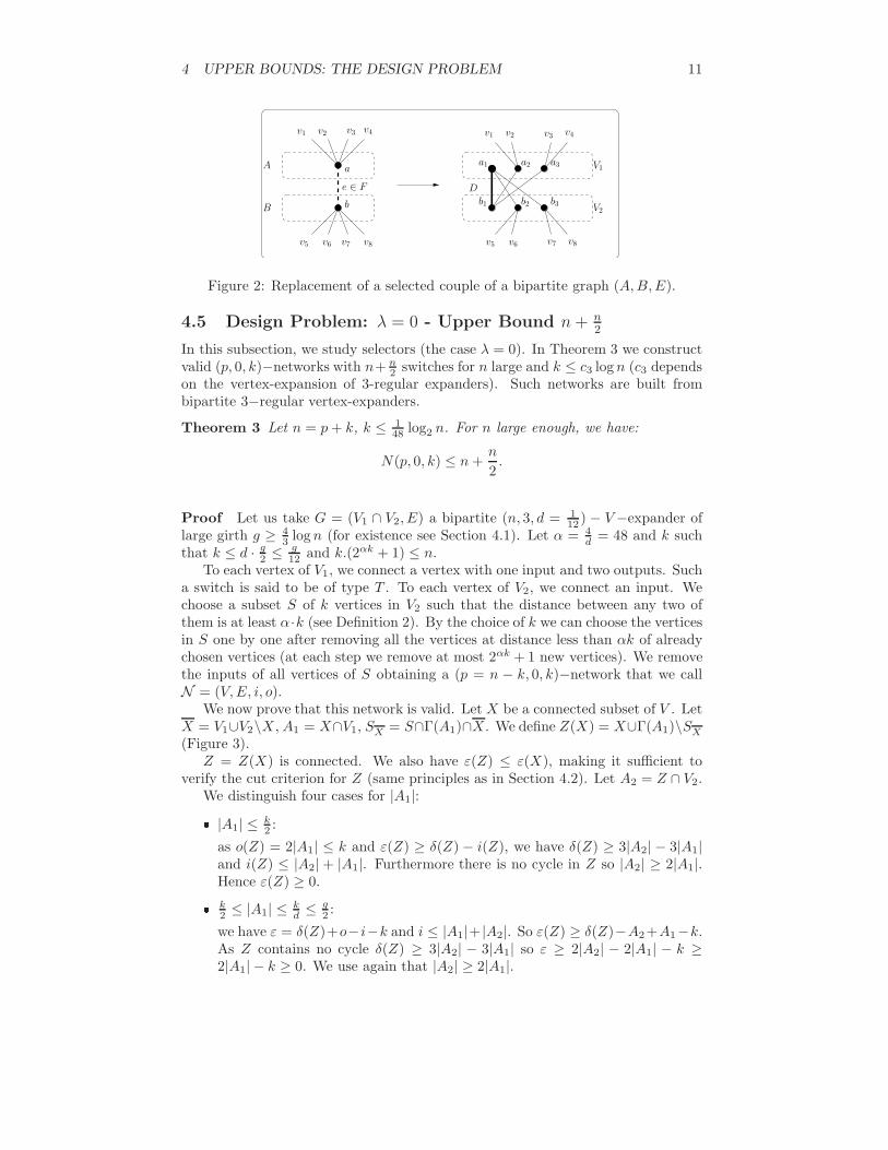
4 UPPER BOUNDS: THE DESIGN PROBLEM 11
v7v6v5 v8
v1
v6v5
v4 v4v3
v8v7
e ∈ F
v1 v2 v3
D
B
A V1
V2
v2
a
b
a3a1 a2
b1 b2 b3
Figure 2: Replacement of a selected couple of a bipartite graph (A, B, E).
4.5 Design Problem: λ = 0 - Upper Bound n + n
2
In this subsection, we study selectors (the case λ = 0). In Theorem 3 we constructvalid (p, 0, k)−networks with n+ n
2 switches for n large and k ≤ c3 log n (c3 dependson the vertex-expansion of 3-regular expanders). Such networks are built frombipartite 3−regular vertex-expanders.
Theorem 3 Let n = p + k, k ≤ 148 log2 n. For n large enough, we have:
N(p, 0, k) ≤ n +n
2.
Proof Let us take G = (V1 ∩ V2, E) a bipartite (n, 3, d = 112 ) − V −expander of
large girth g ≥ 43 log n (for existence see Section 4.1). Let α = 4
d = 48 and k suchthat k ≤ d · g
2 ≤ g12 and k.(2αk + 1) ≤ n.
To each vertex of V1, we connect a vertex with one input and two outputs. Sucha switch is said to be of type T . To each vertex of V2, we connect an input. Wechoose a subset S of k vertices in V2 such that the distance between any two ofthem is at least α·k (see Definition 2). By the choice of k we can choose the verticesin S one by one after removing all the vertices at distance less than αk of alreadychosen vertices (at each step we remove at most 2αk + 1 new vertices). We removethe inputs of all vertices of S obtaining a (p = n − k, 0, k)−network that we callN = (V, E, i, o).
We now prove that this network is valid. Let X be a connected subset of V . LetX = V1∪V2\X , A1 = X∩V1, SX = S∩Γ(A1)∩X. We define Z(X) = X∪Γ(A1)\SX
(Figure 3).Z = Z(X) is connected. We also have ε(Z) ≤ ε(X), making it sufficient to
verify the cut criterion for Z (same principles as in Section 4.2). Let A2 = Z ∩ V2.We distinguish four cases for |A1|: |A1| ≤ k
2 :
as o(Z) = 2|A1| ≤ k and ε(Z) ≥ δ(Z) − i(Z), we have δ(Z) ≥ 3|A2| − 3|A1|and i(Z) ≤ |A2| + |A1|. Furthermore there is no cycle in Z so |A2| ≥ 2|A1|.Hence ε(Z) ≥ 0. k2 ≤ |A1| ≤ k
d ≤ g2 :
we have ε = δ(Z)+o−i−k and i ≤ |A1|+ |A2|. So ε(Z) ≥ δ(Z)−A2+A1−k.As Z contains no cycle δ(Z) ≥ 3|A2| − 3|A1| so ε ≥ 2|A2| − 2|A1| − k ≥2|A1| − k ≥ 0. We use again that |A2| ≥ 2|A1|.

5 GRAPH ROBUSTNESS 12
A1
SX
Γ(A1)v ∈ Su ∈ S
X
F (X)
= X ∪ Γ(A1)
\SX
Figure 3: Sketch of proof of Theorem 3. kd ≤ |A1| ≤ n − k
d :
in this case, ε ≥ δ(Z)−|A2|+|A1|−k and δ(Z) ≥ 3(|A2|−|A1|) = |A2|−|A1|+2(|A2| − |A1|), so we have ε ≥ 2(|A2| − |A1|) − k. Furthermore |A2| − |A1| ≥ΓG(A1)−k, because at most k vertices of ΓG(A1) are in S\A2 (where ΓG(A1)is the neighborhood of A1 in G). By the expansion property, we have:
|ΓG(A1)| ≥ |A1| + d(1 − |A1|/n)|A1|.
In this case d(1− |A1|/n) ≥ 2k. So |ΓG(A1)| − |A1| ≥ 2k. So |A2| − |A1| ≥ k.It implies ε ≥ 0. n − k
d ≤ |A1|:we can assume that Z is connected (see the remarks on Proposition 1). Asthe vertices of S are at distance at least αk with αk > k
d , Z contains at mostone vertex of S. Hence i ≥ |A2| − k +1 + |A1| and ε ≥ δ(Z)− |A2|+ |A1| − 1.Because of the connectivity of Z and the 3−regularity |A2| > |A1|. So ε ≥ 0.
5 Graph Robustness: A New Approach to the De-
sign of Valid Networks
The construction of valid networks is related to a more general expansion propertyof graphs, more precisely to what can be seen as a ’bounded expansion property’ orexpansion property only for sets of bounded size. We call this property robustness.
Definition 3 (α-robustness) The α-robustness, robα, of a graph G is the maximum
value r, such that, for every subset X ⊂ V (G) with |X | ≤ |V |2 , we have δ(X) ≥
min(r, α|X |).
For α = 1 we simply say robustness. There are two main problems: on the onehand we want to understand the behavior of the robustness for a general graph,
5 GRAPH ROBUSTNESS 13
which means giving some upper bounds, for instance showing the existence of sub-sets which violate the α−robustness. This problem covers in particular the classicalproblem of bisection-width, which has several important applications, see for ex-ample [1] and [24]. On the other hand, for many applications, one would like to beable to find graphs of large robustness (α−robustness). The first examples of suchgraphs are expanders of expansion factor c which give graphs with c−robustness atleast n
2 where n is the number of vertices. For d-regular graphs we have:
- if G is d-connected, robd = 1 and robd−1 = 2. robd−2 = g where g is thedouble girth of the graph (minimum size of a cycle with a chord);
- for α ≤ 12 (d − 2
√d − 1), robα ≥ n
2 for Ramanujan graphs;
- for α > d2 − c
√d, where c is some absolute constant depending only on d,
α−robustness is strictly smaller than n2 (see Alon [1]);
- for α > 13 + ǫ the α−robustness of a 3-regular graph is strictly smaller than
n2 , the same is true for α > 4
5 + ǫ and for 4-regular graphs (see Monien-Preis[24]).
Remark that, since it is NP-hard to compute the double girth of a graph, computingrob2(G) is an NP-hard problem. The same is true for any α.
Remark 1 Before going through the study of robustness we would like to stressthat the concept of robustness is closely related to the concept of general selectors.A general selector is a selector without degree conditions. More precisely we havea graph G, such that the set of vertices V (G) is partitioned into three subsets: Ithe set of vertices with one input, O the set of vertices with one output and S theset of normal vertices with neither input nor output, with |I| = p + k and |O| = p.We say that G is a general selector (or is a
(
p+kp
)
-network) if for any subset of Iof size p, there exist p edge-disjoint paths, each one joining one different input toone different output.
Selectors also provide a very natural framework for constructing general validnetworks, i.e., valid networks without degree constraints. For instance, for any(p, λ, k), we can construct a general valid (p, λ, k)-network as follows: take twoselectors, a
(
p+kp
)
-network, A, and a(
p+λp
)
-network, B. Let G be the graphobtained by taking the disjoint union of A and B, deleting the outputs connectedto them, joining the two sets O(A) and O(B) by a matching and replacing theinputs connected to I(B) by outputs. The resulting network is a general valid(p, λ, k)-network in which I(A) is the set of vertices with one input and I(B) is theset of vertices with one output.
In the following, rα denotes the maximum α-robustness of a 4-regular graph.
5.1 Robustness of random 4-regular graphs
In this section G(k, n) is the probability space of all graphs on n vertices thatare the union of k disjoint Hamiltonian cycles, all graphs occurring with the sameprobability. By Gk,n we denote an element of G(k, n). This probability space is”equivalent” to the probability space of random 2k-regular graphs, see [22].

5 GRAPH ROBUSTNESS 14
Theorem 4 Random 4-regular graphs have 1-robustness at least n14 with high prob-
ability, i.e. with probability 1 −O( log nn ).
Corollary 1 For k ≤ n7 , there exist (p, λ, k)−valid networks of size 3n (remember
that n = p + k).
Proof Suppose that a 4−regular Hamiltonian graph G of robustness n7 on 2n
vertices is given. Extract a complete matching from a Hamiltonian cycle and adda doublon to every edge of this matching. It is now straightforward to show thatthe resulting network is valid. This gives a valid (p = n − k, k, k)-network with 3nswitches.
Remark 2 The method of the proof of Theorem 4 can be also used to obtain lowerbounds for α-robustness of random 4-regular graphs for other values of α. Somenumerical results are given below for some special values of α:
- r 1125
= n2 (See Bollobas [15] for another proof of this result).
- r 1120
≥ n2.6 , r 4
5≥ n
5.7 , r 23≥ n
3.6 , r 35≥ n
3 .
Proof [ of Theorem 4] We first give preliminary results on the unions of k disjointHamiltonian cycles. The results for 4-regular graphs are then a direct applicationwith k = 2. Let G be a graph of G(k, n) and S be a subset of V with s vertices. Onthe cycles C1, C2, . . . Ck constituting G, S can be described as a set of continuousintervals. For i = 1, . . . k, let mi(S) be the number of intervals that S defines onCi. Then δ(S) = 2
∑
i=1,2,...k mi(S).For a given cyclic permutation π, if I(s, m) denotes the number of sets of s
elements defining m segments on the cycle associated to π, we have:
Claim 1
I(s, m) =
(
s − 1
m − 1
)(
n − s
m
)
+
(
n − s − 1
m − 1
)(
s
m
)
=
(
s
m
)(
n − s
m
)(
m
s+
m
n − s
)
.
(1)
ProofThe number of ways to write a number t as the ordered sum of p non-negative
integers is cut(t, p) =(
t+p−1p−1
)
. Also, the number of ways to write t as the ordered
sum of p positive integers is cut(t − p, p) =(
t−1p−1
)
.Starting from the vertex 0 of the cycle, the set S can be encoded by giving two
sequences of numbers : the ordered list of the lengths of the segments in S and theordered list of the lengths of the segments in S. There are two cases, depending onwether the first interval belongs to S or to S. If 0 belongs to S, then S is associated with exactly m segments on the path,
all having length at least 1, and S is associated to m + 1 segments, all butthe last one having length at least 1 (the last segment can have length 0).
So S can be encoded by dividing |S|−m = n−s−m into m+1 non-negativeintegers. There are exactly cut(n − s − m, m + 1) ways of doing it.
We should also write S as the ordered sum of m non null numbers, there arecut(s − m, m) =
(
s−1m−1
)
possibilities.
This gives a contribution of cut(n−s−m, m+1) ·cut(s−m, m) =(
s−1m−1
)(
n−sm
)
to I(s, m).

5 GRAPH ROBUSTNESS 15 If 0 is in S, the situation is symmetric, with n − s instead of s: we replacecut(n− s−m, m + 1)cut(s−m, m) by cut(s−m, m + 1)cut(n− s−m, m) =(
sm
)(
n−s−1m−1
)
.
The total contribution is the sum of the partial contributions, and the claim follows.
Given a set S with s elements, we denote by P (s, m) the probability that for arandom cyclic permutation π, S defines m segments on the cycle associated to π.Since the probability does not depend on S, but only on s, P (s, m) is well defined.We have:
Claim 2
P (s, m) = I(s, m)/
(
n
s
)
=
(
sm
)(
n−sm
)
(ms + m
n−s )(
ns
) . (2)
Proof Consider a bipartite graph whose vertices are the sets of s elements and the(n−1)! cyclic permutations. We put an edge between a set and a cyclic permutationif the set defines m segments on the cycle associated to the permutation. Thisgraph is a “regular bipartite graph”, where sets have degree ∆ and permutations
have degree I(s, m). Counting the edges of the graph, we get ∆ = (n−1)!I(s,m)
(n
s).
Now, the probability for a set to be adjacent to a permutation is ∆/(n−1)!. So,given a set S with s elements, the probability that S defines exactly m segmentson a cycle C is I(s, m)/
(
ns
)
. Then Equation 1 gives the result.
Claim 3
Prob(δ(S) = 2x) =∑
k1,...,kk|k1+k2+...+kk=x
∏
I(s, ki)/
(
n
s
)k
. (3)
Proof The result follows from the three points below: the probability that S defines ki segments on a random cycle Ci is I(s, ki); the cycles constituting Gk,n are independent δ(S) = 2∑
1,2,...,k ki.
We say that a set is bad if δ(S) < min(s, n − s, r). By the above equations we canestimate the probability of having bad sets. The following two lemmas completethe proof of our Theorem.
Lemma 2 (Robustness for small sets) Any set with size s ≤ n14 has border at
least s with probability 1 −O( log nn ).
ProofThe number of cycles is two for 4-regular graphs. Let W (n, s) be the probability
that there is a set of size s ≤ r = n14 with border less than s:
W (n, s) ≤(
n
s
)
∑
r≤s/2
∑
m1+m2=r
I(s, m1)I(s, m2)/
(
n
s
)2
.

5 GRAPH ROBUSTNESS 16
Since I(s, m1)I(s, m2) ≤ I(s, m1+m2
2 ), we have
W (n, s) =∑
r≤s/2
∑
m1+m2=r
I(s, m1)I(s, m2)/
(
n
s
)
≤∑
r≤s/2
r(I(s, r/2))2/
(
n
s
)
.
Now, since r ≤ s/2, we have I(s, r/2) ≤ I(s, s/4) and W (n, s) ≤ s2
8 (I(s, s/4))2/(
ns
)
.Replacing I(s, s/4) by its value we get:
W (n, s) ≤ s2
8
(
s
s/4
)2 (n − s
s/4
)2
/
(
n
s
)
.
For the following we need the following rather sharp form of Stirling’s formulaproved by Robbins(1955):
n! =(n
e
)n √2πneαn ,
where 112n+1 < αn < 1
12n .Putting this formula in the above inequality we obtain:
W (n, s) ≤ s3s(n − s)3n−3s
( s4 )s(3s
4 )3s2 (n − 5s
4 )2n− 5s2 nn
β,
where β =16 (n−s)
√s(n−s)
3π√
2πn (4n−5s).eγ with
γ = 3αs + 3αn−s − 4α s4− 2α 3s
4− 2αn− 5s
4− αn,
αi being a real number in the interval [ 112i+1 , 1
12i ]. Let
X(n, s) :=s3s(n − s)3n−3s
( s4 )s(3s
4 )3s2 (n − 5s
4 )2n− 5s2 nn
β.
Suppose n = a · s. Then we have:
X(n, s) =
(
(a − 1)3(a−1)
14 .(3
4 )32 .(a − 5
4 )2a− 52 .aa
)s
β.
If we note
g(a) :=(a − 1)3(a−1)
14 .(3
4 )32 .(a − 5
4 )2a− 52 .aa
,
we haveX(n, s) = g(a)s.β.
Remember that
β =16 (n − s)
√
s(n − s)
3π√
2πn (4n − 5s).eγ .
It is now easy to see that g is decreasing. As g(13.80 · · · ) = 1, we have g(14) < 1.Hence

5 GRAPH ROBUSTNESS 17 For s ∈ [− 4 log nlog(g(14)) ,
n14 ] we have
X(n, s) ≤ C.1
n4β = O(
1
n2),
for some constant C. Hence for some other constant C,
W (n, s) ≤ C.1
n2. For s ≤ − 4 log n
log(g(14)) we have a ≥ C. nlog n (for some constant C). Hence
X(n, s) ≤ C.(n/s)−s2 .β.
It is clear that for s ≥ 4, we have X(n, s) ≤ C. 1n for some constant C. It is easy to show that W (n, s) = 0 for s = 1, 2, 3, as the edge connectivity of
a random 4-regular graph is 4 with very high probability.
Then we have∑
s≤ n14
W (n, s) ≤∑
− 4 log n
log(g(14)) ≤s≤ n14
X(n, s) +∑
s≤− 4 log n
log(g(14))
X(n, s)
< C.n.1
n2+
C. log(n)
n= O(
log n
n).
Lemma 3 (Robustness for large sets) For n large enough, any set of size s ∈[ n14 , 13n
14 ] has border at least n14 with probability 1 −O( 1
n ).
ProofA set larger than n
14 is bad when its border is smaller than n14 . Let W ′(n, s)
be the probability that there exists a set of size s ≥ r = n14 with border less than
r = n14 . We have
W ′(n, s) ≤∑
i≤ n28
∑
k1+k2=i
I(s, k1)I(s, k2)/
(
n
s
)
.
Hence W ′(n, s) ≤ ( n14 )2
8
(
I(s, n56 ))2
/(
ns
)
.
Let define δ(a) for a ∈ [ 114 , 1 − 1
14 ] as
δ(a) =
(
(
a.nn56
)(
(1−a)nn56
)
)2
(
na.n
) .
Then
W ′(n, an) ≤ 1
8
( n
14
)2
δ(a).
Again, using methods similar to the ones of last section, we obtain W ′(n, a) ≤h(a)nβ′, where β′ is a rational function on n and a, and h is defined below:
h(a) =a3a (1 − a)3−3a
( 156 )
114 (a − 1
56 )2a− 128 (1 − a − 1
56 )2−2a− 128
β′.

6 LOWER BOUNDS 18
Since h( 114 ) < 1, with h decreasing,
W ′(n, an) ≤ h(1
14)nβ′.
As β′ is rational, we have for n large enough W ′(n, an) < 12n2 , and so W ′(n, s) =
O( 1n ). So
∑
s∈[ n14 , 13n
14 ]
W ′(n, s) = O(1
n),
and the lemma is proved.
6 Lower Bounds
In this section we distinguish switches according to their number of inputs andoutputs. Figure 4 defines the different set of switches: S, Si, So, Vi, Vo, D andT . For example, a switch v is in D if i(v) = o(v) = 1. Remember that we calledsuch a switch a doublon and that all switches that are not a doublon are calledR-switch. Remark that direct applications of the cut criterion show that no othertypes of switches are possible and that, as soon as λ ≥ 1, switches of kind T areforbidden. Recall the convention that a lower case letter in the notations indicatesthe cardinality of the set denoted by the corresponding upper case letter.
DViS Si So TVo
Figure 4: Kinds of switches.
Fundamental equations are linking the different kinds of switches: Equation 4(switch partition equation) which counts the number N of switches of the network,Equation 5 (input equation) which counts the number of inputs and Equation 6(output equation) which counts the number of outputs.
N = s + si + so + d + vi + vo + t (4)
p + λ = si + 2vi + d + t (5)
p + k = so + 2vo + d + 2t (6)
In Subsection 6.1, we prove a fundamental preliminary theorem, Theorem 5. Itsmain point is that N(p, λ, k) ≥ 3
2n + d2 − ε(n) (where d is the number of doublons
and where ε(n) goes to zero when n goes to infinity). Direct applications of thistheorem give lower bounds for general and simplified networks (Theorems 6 and7). We succeed in obtaining a better bound of n + 2
3n − ε(n) for two cases: whenλ goes to infinity (Theorem 8) and when some kinds of switches are not allowedin the networks (Theorem 9). Finally (Theorem 10), we succeed to obtain a tightbound n + 3
4n − ε(n) for another family of networks using majority arguments.
6 LOWER BOUNDS 19
6.1 Preliminary Theorem
The idea to find and prove lower bounds here is first to obtain local informationon possible switch configurations. The methodology is to use the cut criterion(Proposition 1) to infer equations linking the numbers of switches of different kinds.Then, we use the existence of a quasi-partition (Lemma 4) to obtain bounds for thewhole network.
Definition 4 (q-quasi-partition) Let G = (V, E) be a graph and q be a positiveinteger. A q-quasi-partition of G is a family Q = A1, A2, . . . , Am of subsets ofV , such that :
(i) for every 1 ≤ i ≤ m, the subgraph G[Ai] induced by Ai is connected;
(ii) for every 1 ≤ i ≤ m, q3 ≤ |Ai| ≤ q;
(iii) V =⋃m
i=1 Ai and∑m
i=1 |Ai| ≤ |V | + |Ai; |Ai| > 2q3 | + 1.
Lemma 4 ([20]) Let q be a positive integer and G be a connected graph of orderat least q
3 . Then G admits a q-quasi-partition.
Remark 3 If G has several connected components, each of size at least q2 ,
applying the lemma to each component and using the additivity of both sidesof Equation (iii) gives us a q−quasi-partition of G. Let Q be a quasi-partition of G as in Lemma 4. Let t = |Ai, |Ai| ≥ 2q
3 | and
v = |V |. Then we have: m ≤ 3(v+t+1)q and t ≤ v+1
2q3 −1
.
Proof The lemma as stated in [20] is slightly incorrect. Hence we restate it hereand give a new proof. Since every connected graph G contains a spanning tree, it issufficient to prove the result for trees. We prove this by induction on the size of thetrees. Let T be a tree. If T contains less than q elements, then the result triviallyholds. So suppose that |T | ≥ q. An edge e of T is called a q-balanced separator, ifremoving e separates the tree into connected components of sizes at least q. Let Eq
be the subgraph consiting of all q-balanced edges. If there is no q-balanced edge inthe tree, a q-separator vertex exists, that is a vertex v such that all the connectedcomponents of T \ v have less than q vertices. Let us take l to be a leaf of Eq ifsome q-balanced edges exist or a q-separator vertex if Eq = ∅. T \ (Eq ∪ l) hasr connected components, say C1, . . . , Cr, such that |C1| ≥ |C2| ≥ · · · ≥ |Cr|. Bythe choice of l, and our hypothesis on the size of T (|T | > q), we have |Ci| < q and∑r
i=1 |Ci| ≥ q. The following cases can appear. |C1| ≥ q3 and T \ C1 has at least q
3 vertices. Then by induction it has a q-quasi partition A1, . . . , Am−1. Adding Am = V (C1) to this family providesa q-quasi partition for T . |C1| < q
3 . We have r ≥ 3. Let s be the largest integer such that∑
i≤s |Ci| ≤ q.
As |Cs+1| ≤ |C1| < q3 , we have s ≥ 3 and
∑
i≤r |Ci| ≥ 2q3 (by maximality of
s).
So we can suppose that∑
i≤r |Ci| ≥ 2q3 . If the connected tree T \ ⋃i≤s Ci
has more than q3 elements, for example if Eq 6= ∅, by induction it admits a
q-quasi partition A1, . . . , Am−1. Adding Am =⋃
i≤s Ci ∪ l to this familyprovides a q-quasi partition for T .
6 LOWER BOUNDS 20 T has less than q + q3 vertices, Eq is empty and we can find a vertex l such
that each |Ci| has less than q3 vertices. Let t be the smallest integer such
that∑
i≤t |Ci| ≥ q3 . We claim that T \⋃i≤t Ci has at most q and at least q
3vertices. The first one is true because T has at most q+ q
3 vertices and⋃
i≤t Ci
has at least q3 vertices. The second one is true, because of the minimality of
t. Indeed,⋃
i≤t−1 Ci has at most q3 vertices, Ct has at most q
3 vertices, andso because |T | ≥ q + 1, T \⋃i≤t Ci has at least q
3 vertices. It is now easy tocheck that
⋃
i≤t Ci ∪ l and T \⋃i≤t Ci form a q-quasi partition of T .
For the proof of Theorem 5 we need to define large and small H−componentsof R, the associated graph of N .
Definition 5 [H-component, large and small H-components, adjacent H-components] We consider a (p, λ, k)-network and its associated graph R (see Sec-tion 2 for definition). We take H the subgraph of R which contains only the edges oftype E0. An H-component of R is a connected component of H. An H-componentis said large (respectively small) if it has more than (resp. strictly less than) qswitches, with q the greatest integer satisfying 2(q +(2q +2)q)+2 ≤ k− 1. Remark
that q ∼√
k2 . Two H-components C1 and C2 are said adjacent if there exists an
edge of R with one R−switch in C1 and the other in C2.
Proposition 2 1. A small H-component has no outgoing edge of kind E2.
2. A small H-component has no input inside.
3. Two small H-components are not adjacent.
Proof Let C be a small H-component. We apply the cut criterion of Section 4.2to the set C of N obtained from C by adding in N the doublons of the edges oftype E1 and E2 incident to R−switches of C.
As k ≤ p and |C| ≤ q ≈√
k2 , we have o(C) ≤ k
2 ≤ p. Hence the cut criterionreduces to
δ(C) ≥ i(C).
Let e1 (res. e2) be the number of outgoing edges of kind E1 (resp. E2) incident toR−switches of C.
- By definition of H and of the small components, δ(C) = e1 + e2. We havei(C) ≥ e1+2e2+i(C). So by the cut criterion, e2 = 0 proving 1) and i(C) = 0proving 2).
- Let C′ be an other small H−component. If C and C′ are joined by f ≥ 1edges, then let W = C∪C′, we have i(W ) ≥ e1+e′1−f and δ(W ) ≤ e1+e′1−2fso δ(W ) < i(W ), giving a contradiction.
Theorem 5 (Preliminary Theorem) In a valid network N with k ≤ n2 , we have
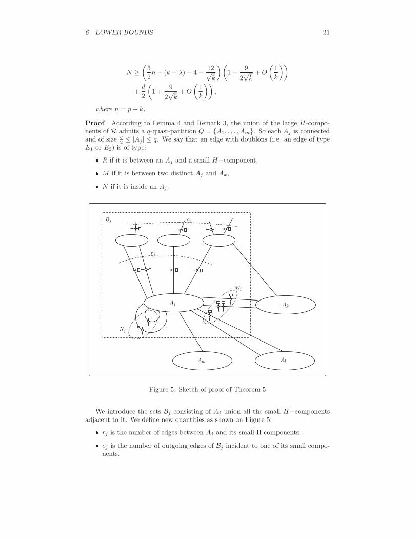
6 LOWER BOUNDS 21
N ≥(
3
2n − (k − λ) − 4 − 12√
k
)(
1 − 9
2√
k+ O
(
1
k
))
+d
2
(
1 +9
2√
k+ O
(
1
k
))
,
where n = p + k.
Proof According to Lemma 4 and Remark 3, the union of the large H-compo-nents of R admits a q-quasi-partition Q = A1, . . . , Am. So each Aj is connectedand of size q
2 ≤ |Aj | ≤ q. We say that an edge with doublons (i.e. an edge of typeE1 or E2) is of type: R if it is between an Aj and a small H−component, M if it is between two distinct Aj and Ak, N if it is inside an Aj .
Aj
rj
Bj ej
Mj
Nj
Ak
AlAm
Figure 5: Sketch of proof of Theorem 5
We introduce the sets Bj consisting of Aj union all the small H−componentsadjacent to it. We define new quantities as shown on Figure 5: rj is the number of edges between Aj and its small H-components. ej is the number of outgoing edges of Bj incident to one of its small compo-
nents.

6 LOWER BOUNDS 22 Mj is the number of doublons on the edges of type M . Nj is the number of doublons on the edges of type N .
As two small components can not be adjacent, remark that all rj and ej edges areof type R.
Let us now apply the cut criterion to Bj. δ(Bj) + o(Bj) − min(k, o(Bj)) −min(i(Bj), p) ≥ 0. As k ≤ n
2 , we have i(Bj) ≤ p. We first show that o(Bj) < k.Indeed, if o(Bj) ≥ k, the cut criterion reduces to δ(Bj) ≥ k. Furthermore Aj isconnected and of size less than q, so it has at most 2q + 2 outgoing edges and thenumber of small H−components of Bj is at most 2q + 2. As the size of a smallH−component is less than q, the number of vertices in Bj is at most q + (2q + 2)q.Hence the number of outgoing edges δ(Bj) is at most 2(q + (2q + 2)q) + 2. By ourchoice of q it gives k ≤ δ(Bj) ≤ 2(q + (2q + 2)q) + 2 ≤ k − 1, a contradiction.Consequently o(Bj) < k.
The cut criterion is now equivalent to δ(Bj) ≥ i(Bj). Noting δ′ the numberof outgoing edges of Bj incident to Aj , we have δ(Bj) = δ′(Bj) + ej . Using thedefinitions of switch kinds (Figure 4), we have
δ′ = 4|Aj | − 2e(Aj) − rj − 2Nj − si − so − 2vi − 2vo − 3t.
Since Aj is connected, e(Aj) ≥ |Aj | − 1, we get
δ′ ≤ 2|Aj | + 2 − rj − 2Nj − si − so − 2vi − 2vo − 3t.
For the number of inputs in Bj we have
i(Bj) = ej + rj + Mj + Nj + si + 2vi + t.
The cut criterion (Proposition 1) then implies:
2|Aj | + 2 ≥ 2si + so + 4vi + 2vo + 4t + 3Nj + 2rj + Mj. (7)
The total number of doublons is d. All doublons are of type R, M or N . Thedoublons in M are counted for two different Aj and Ak. So
∑mj=1 Mj +3Nj +2rj ≥
2d. Hence taking the sum of Equation 7 over all j we obtain
2
m∑
j=1
|Aj | + 2m ≥ 2si + so + 4vi + 2vo + 4t + 2d.
The input and output equations (Equations 5 and 6) give 2si + 4vi + 2t + 2d =2n − 2(k − λ) and so + 2vo + 2t = n − d. Hence
2
m∑
j=1
|Aj | + 2m ≥ 3n − d − 2(k − λ). (8)
The family Aj forms a q-quasi-partition of R. Let t := |Aj , |Aj | ≥ 2q3 | and v the
number of vertices of R. Then, by Remark 3, we have m ≤ 3(v+t+1)q and t ≤ v+1
2q
3 −1.
By definition of a quasi-partition:∑m
i=j |Aj | ≤ v + |Aj , |Aj | ≥ 2q3 | = v + t + 1.
Putting all these equations into Equation 8 gives:
2v
(
1 +1
2q3 − 1
)
≥ q
q + 3[(3n − d − 2(k − λ)) − 2(q + 3)
q− 6
q− 2].
6 LOWER BOUNDS 23
2v ≥ q
q + 3
2q − 3
2q[3n − d − 2(k − λ) − 2(q + 3)
q− 6
q− 2]
= [3n − d − 2(k − λ) − 2(q + 3)
q− 6
q− 2]
(
1 − 9
2q + 6
)
.
Using N ≥ v + d, we obtain
N ≥(
3
2n − (k − λ) − 4 − 12
q
)(
1 − 9
2q + 6
)
+d
2
(
1 +9
2q + 6
)
.
Finally,
N ≥(
3
2n − (k − λ) − 4 − 12√
k
)(
1 − 9
2√
k+ O
(
1
k
))
+d
2
(
1 +9
2√
k+ O
(
1
k
))
.
6.2 Lower Bounds
Here we apply Theorem 5 to prove lower bounds for the number of switches of min-imal valid networks. Let us remind the reader that l ≤ k is assumed for symmetryreasons and that n := p + k.
Theorem 6 (Selector: λ = 0) In a valid network N , when k → ∞ with k ≤ n2 ,
we haveN ≥ n +
n
2+ O(
n√k
).
In other words,
N(p, 0, k) ≥ n +n
2+ O(
n√k).
In particular, we obtain a tight bound for networks with λ = 0 (see Theorem 3).
Proof The proof follows directly from Theorem 5.
Theorem 7 (Simplified case) In the simplified case, when k → ∞ with k ≤ n2 ,
we have N(p, λ, k) ≥ 2n + O( n√k).
In particular, we obtain a tight bound for the simplified case (see Theorem 1).
Proof First recall that a direct application of the cut criterion shows that as soonas λ ≥ 1, T is empty (see definition of switch types in Figure 4, p. 18). This meansthat in this proof and the following we will not consider switches of T . Now theproof follows from Theorem 5 and from d = n − (k − λ) in the simplified case.
Theorem 8 (General case) When λ → ∞ and k → ∞, N(p, λ, k) ≥ n + 23n +
O( n√λ).
Proof We first give a bound for the number of switches of types Vi and Vo usingthe following remark:

6 LOWER BOUNDS 24
Figure 6: When λ = 0, switches of kind Vi may be removed.
Lemma 5 When λ → ∞ and k → ∞,
vi ≤ N − 32n − d
2 − k−λ2 + λO( n√
k),
vo ≤ N − 32 (n − k + λ) − d
2 + k − λ−k2 + O( n√
λ).
Proof Imagine we have a valid (p, λ, k)−network with N switches and vi switchesin Vi. We obtain a valid (p, 0, k)−network after removing any λ inputs. This newnetwork has at least vi −λ switches of kind Vi. By Remark 4 we may remove theseswitches and obtain a valid (p, 0, k)−network with N − vi + λ switches. Theorem 5gives
N − vi + λ ≥ 3
2n +
d
2+
k − λ
2+ O(
n√k
).
So the result holds. Symmetry (in the sense of swapping inputs and outputs givesa valid (p, k, λ)−network) gives the second equation.
The switch partition equation and Equations 5 and 6 give here
N = 2n − (k − λ) − vi − vo − d + s.
Lemma 5 gives
N ≥ 2n − (k − λ) − d + s − 2N + 3n + d
+ O(n√k
) + O(n√λ
) − 3
2(k − λ) − λ − k.
N ≥ 5
3n + O(
n√k
) + O(n√λ
) − 5
2k +
λ
2.
Theorem 9 When λ ≥ 1 and no switches of kinds Vi and Vo are allowed, whenk → ∞ with k ≤ n
2 , we have N(p, λ, k) ≥ n + 23n + O( n√
k).
Proof Let us first remark the following:
Remark 4 Notice that when λ = 0, switches of type Vi are not present in aminimal valid (p, λ, k)−network. As shown in Figure 6, they may be removed toform a new valid (p, λ, k)−network with vi less switches.
Proof Direct by the cut criterion.

6 LOWER BOUNDS 25
When vi = vo = 0, the input equation (Equation 5) becomes n = d + si and theoutput equation (Equation 6) becomes n = d + so. So si = so and the switchpartition equation (Equation 4) gives
N = 2n − d. (9)
Theorem 5 gives
2n − d ≥ 3
2n +
d
2+ O(
n√k
)
n
3≥ d + O(
n√k
).
Equation 9 gives
N ≥ 5
3n + O(
n√k
).
To sum up, in the general case, we proved a lower bound of type n + 2n/3. Letus remind the reader that we obtained an upper bound with n + 3n/4 switches(Theorem 2). We conjecture that the later is the right answer to the problem. Weare able to prove this with some extra conditions on the network using majorityarguments:
Theorem 10 Let N be a network of N switches with the associated graph R =(V = A ∪ B, E) such that R is bipartite, all vertices of A have exactly one outputand all vertices of B exactly one input in the original network.
N ≥ n +3
4n + O(
n√k).
Proof We are given a ternary bipartite graph R = (V = A ∪ B, E) such that allvertices of A have an output and all vertices of B have an input. The vertices ofB are partitioned in two sets B1 and B0. A vertex of B1 is adjacent to an edge oftype E1 or E2, while the vertices of B0 are not.
For a subset X ⊂ A we use the following notations : Bi(X) = Γ(X)∩Bi, i = 0, 1and bi = |Bi|.
Let X be a subset of A such that F (X) = X ∪Γ(X) is connected and 6|X | ≤ k.X has less than k outputs. To fullfill the cut criterion for small subsets (less thank outputs), we need
b0(X) ≥ b1(X) − 3 + 3cF (X), (10)
where cF (X) is the feedback edge set of the subgraph induced by F (X).
The goal is to prove that this can happen only if b0 + O( 1√k) ≥ 2b1.
Let Y be a set of y vertices of B0 such that Y ∪ Γ(Y ) is connected. We have|Γ(Y )| = 2y + 1− cF (Y ). There are 3y + 3− 3c edges comming out of F (Y ), say αytoward vertices of type B0 and 3y+3−3c−αy toward vertices of type B1. In G weconsider the connected subgraph induced by Z = F (Y )∪ (Γ(F (Y ))∩B1). We have(6− α)y + 3− 3cF (Y ) edges inside Z, so the number of vertices in Γ(F (Y )) ∩B1 is
7 CONCLUSION 26
(6 − α)y + 3 − 3cF (Y ) − y − (2y + 1− cF (Y )) − cZ = (3 − α)y + 2 − 2cF (Y ) − cZ . Ifwe take X = Γ(Y ), Equation 10 gives
(α + 1)y ≥ b0(X) ≥ b1(X) − 3 + 3cF (X)
≥ (3 − α)y + 2 − 2cF (Y ) − cZ − 3 + 3cF (X)
≥ (3 − α)y − 1 − 2cF (Y ) + 2cF (X)
where in the last inequality we use the fact that cZ ≤ cF (X). As cF (Y ) ≤ cF (X), wehave:
α ≥ 1 − 1
2y.
We consider all the connected components of the graph induced by B0 ∪A andwe take a q-quasi-partition of the big components for some q, q = O(k) such thatall components are of the form F (Y ) for some Y subset of B0. Now we count theedges going to B0 and B1.
For one component D of the quasi-partition with y vertices of B0, we find atleast (3 + α)y ≥ 4y − 1
2 edges toward B0 and at most 2y + 72 edges toward B1 with
one extremity in D.Globally, if m is the number of components and up to some small number of
recounting (Quasi-partition arguments) we get 4|A| − m2 = 3b0 edges toward B0
and 2A + 7m2 = 3b1 edges toward B1.
Hence b0 ≥ 2b1 + O( 1√k).
7 Conclusion
In this paper we proposed constructions of valid (p, λ, k)−networks and gave lowerbounds on their size. The design problem appears to be driven by two constraints:a local one in which small patterns are forbidden and another one which is relatedto some global expansion property of the network. This led us to define an expan-sion parameter of a graph: the α−robustness. This parameter is a generalization ofthe usual edge-expansion. Using graphs of 2−robustness equal to Θ(log n) we con-structed almost optimal simplified networks. Similarly when k ≤ n
7 , using graphs oflarge 1−robustness we proposed good simplified networks. Despite many answersfor small values of k (k ≤ n
7 ), little is known when k is larger.To obtain our lower bounds, we presented a powerful technique: quasi-partitioning.We think that this technique can potentially have other applications to derive lowerbounds for problems of the same kind.
Some interesting open questions remain
- For a fixed α, find explicit constructions of nice α-robust graphs, graphshaving large α−robustness.
- Is there a very explicit construction such as the “Zig-Zag product”of [29] and“lift”of [13] providing nice robust graphs? Does the Zig-Zag product preserverobustness?
- What is the maximum bisection-width of a 4-regular graph? In [24] themaximal bisection width of 4-regular graphs on n vertices is shown to be atmost 2n
5 . This leads to an α−robustness < n2 when α > 4
5 . Is it possible to

8 ACKNOWLEDGMENTS 27
obtain the same kinds of results for larger values of α ensuring a maximalrobustness of size at most n
3 , for example?
- What is the minimum number of switches or edges in an n-superselector? (See[23, 30] for some constructions.)
8 Acknowledgments
We are grateful to the anonymous referees for their valuable remarks which helpedus to improve the presentation of our results. We especially thank Networks’ Editor-in-Chief Douglas Shier for his helpful comments on earlier versions of this paper.We also want to acknowledge Jean-Claude Bermond and Frederic Havet for theirinterest in our work.
References
[1] N. Alon, On the edge-expansion of graphs, Combin, Probability Comput 11 (1993),1–10.
[2] N. Alon and M. Capalbo, Smaller explicit superconcentrators, Proc 14th Ann SympDiscret Algorithms ACM-SIAM SODA, 2003, pp. 340–346.
[3] N. Alon, Z. Galil, and V.D. Milman, Better expanders and superconcentrators, JAlgorithms 8 (1987), 337–347.
[4] N. Alon, P. Hamburger, and A.V. Kostochka, Regular honest graphs, isoperimetricnumbers, and bisection of weighted graphs, Eur J Combin 20 (1999), 469–481.
[5] N. Alon and V.D. Milman, Eigenvalues, expanders and superconcentrators, Proc25th Ann Symp Fondations Comput Sci (FOCS), Singer Island, Florida, 1984, pp.320–322.
[6] L.A. Bassalygo, Asymptotically optimal switching circuits, Problemy Pederachi In-formatsii 17 (1981), 81–88.
[7] B. Beauquier and E. Darrot, Arbitrary size Waksman networks, Premiere rencontresfrancophones sur les aspects algorithmiques de telecommunication (Algotel), 1999,pp. 95–100.
[8] B. Beauquier and E. Darrot, Arbitrary size Waksman networks and their vulnerabil-ity, Parallel Process Lett 3-4 (2002), 287–296.
[9] J.C. Bermond, E. Darrot, and O. Delmas, Design of fault tolerant on-board networksin satellites, Networks 40 (2002), 202–207.
[10] J.C. Bermond, O. Delmas, F. Havet, M. Montassier, and S. Perennes, Reseaux detelecommunications minimaux embarques tolerants aux pannes, Cinquieme rencon-tres francophones sur les aspects algorithmiques de telecommunication (Algotel),2003, pp. 27–32.
[11] J.C. Bermond, F. Giroire, and S. Perennes, Design of minimal fault tolerant on-boardnetworks : Practical constructions, 14th Int Colloq Structural Informat CommunComplexity (SIROCCO), Lecture Notes in Comput Sci, Springer, 2007, Number 4474pp. 261–273.
[12] J.C. Bermond, F. Havet, and C.D. Toth, Fault tolerant on-board networks withpriorities, Networks 47 (2006), 9–25.
[13] Y. Bilu and N. Linial, Lifts, discrepancy and nearly optimal spectral gaps, Combina-torica 26 (2006), 495–519.

REFERENCES 28
[14] M. Blum, R. Karp, C. Papadimitriou, O. Vornberger, and M. Yannakakis, The com-plexity of testing whether a graph is a superconcentrator, Informat Process Lett 13(1981), 164–167.
[15] B. Bollobas, The isoperimetric number of random regular graphs, Eur J Combin 9,3 (1988), 241–244.
[16] M. Capalbo, O. Reingold, S. Vadhan, and A. Wigderson, Randomness conductorsand constant-degree lossless expanders, 34th ACM Symp Theory Comput (STOCS),2002, pp. 659–668.
[17] F.R.K. Chung, On concentrators, superconcentrators, generalizers and nonblockingnetworks, Bell System Tech J 58 (1979), 1765–1777.
[18] F.R.K. Chung, Spectral Graph Theory, American Mathematical Society, 1997.
[19] G. Davidoff, P. Sarnak, and A. Valette, Elementary number theory, group theory,and Ramanujan graphs, Cambridge University Press, 2003.
[20] O. Delmas, F. Havet, M. Montassier, and S. Perennes, Design of fault tolerant on-board networks, INRIA Res Report 5866, submitted (2006).
[21] F. Giroire, Reseaux, algorithmique et analyse combinatoire de grands ensembles,Ph.D. Thesis, Universite Paris VI, November 2006.
[22] C. Greenhill, J.H. Kim, and N.C. Wormald, Hamiltonian decompositions of randombipartite regular graphs, J Combinatorial Theory Ser B 90 (2004), 195–222.
[23] F. Havet, Repartitors, selectors and superselectors, J Interconnection Networks 7(2006), 391–415.
[24] B. Monien and R. Preis, Upper bounds on the bisection width of 3-and 4-regulargraphs, J Discr Algorithms 4 (2006), 475–498.
[25] M. Morgenstern, Existence and explicit constructions of q + 1 regular Ramanujangraphs for every prime power q, J Combinatorial Theory Ser B 62 (1994), 44–62.
[26] M. Murty, Ramanujan graphs, J Ramanujan Math Soc 18 (2003), 33–52.
[27] H.Q. Ngo and D. Du, Notes on the complexity of switching networks, Advancesin Switching Networks, Kluwer Academic Publishers, Dordrecht, The Netherlands,(2001), pp. 307–367.
[28] N. Pippenger, Superconcentrators, SIAM J Comput 6 (1977), 298–304.
[29] O. Reingold, S. Vadhan, and A. Wigderson, Entropy waves, the zig-zag graph prod-uct, and new constant-degree expanders and extractors, Ann Math 155 (2002), 157–187.
[30] U. Schoning, Smaller superconcentrators of density 28, Informat Process Lett 98(2006), 127–129.
[31] L.G. Valiant, On non-linear lower bounds in computational complexity, 7th ACMSymp Theory Comput (STOCS), 1975, pp. 45–53.

162 Annexes

Annexe B
Algorithmes de routage
B.1 (ℓ,k)-Routing on Plane Grids
Article soumis à Journal of Interconnectio Networks.
B.2 On Multiple Improper Colorings
Article en préparation.
B.3 The Proportional Colouring Problem : OptimisingBuffers in Radio Mesh Networks
Article soumis à un numéro spécial de Discrete Applied Mathematics.
163

appor t de r ech er ch e
ISS
N02
49-6
399
ISR
NIN
RIA
/RR
--64
80--
FR
+E
NG
Thème COM
INSTITUT NATIONAL DE RECHERCHE EN INFORMATIQUE ET EN AUTOMATIQUE
(ℓ, k)-Routage dans les Grilles Planaires
Omid Amini — Florian Huc — Ignasi Sau — Janez Žerovnik
N° 6480
February 2008


Unité de recherche INRIA Sophia Antipolis2004, route des Lucioles, BP 93, 06902 Sophia Antipolis Cedex (France)
Téléphone : +33 4 92 38 77 77 — Télécopie : +33 4 92 38 77 65
(ℓ, k)-Routage dans les Grilles Planaires ∗Omid Amini † , Florian Hu ‡ , Ignasi Sau ‡ § , Janez erovnik ¶ ‖Thème COM Systèmes ommuni antsProjet MASCOTTERapport de re her he n° 6480 February 2008 33 pagesRésumé : Le problème de routage de paquets joue un rle très important dans les réseauxde télé ommuni ation. Il onsiste à envoyer des données entre les sommets d'un réseau enun temps raisonable. Dans le (ℓ, k)-routage, haque sommet peut envoyer au plus ℓ paquetset en re evoir k. Le routage de permutation orrespond au as ℓ = k = 1. Dans le routager- entral, tous les noeuds à distan e au plus r d'un sommet xé envoient un paquet à esommet. Dans et arti le nous étudions les problèmes pré édents dans les grilles planaires.On utilise le modèle store-and-forward et ∆-port. Nous onsidérons les réseaux half et full-duplex. Les résultats prin ipaux sont :1. un algorithme tight pour le problème de routage de permutation dans les grilles hexa-gonales full-duplex, et dans les grilles hexagonales et triangulaires half-duplex.2. un algorithme tight pour le routage r- entral dans les grilles triangulaires et hexago-nales.3. un algorithme tight pour le (ℓ, ℓ)-routage dans les grilles arrées, triangulaires et hexa-gonales.4. de bon algorithme d'approximation (en terme de temps de al ul) pour le (ℓ, k)-routage dans les grilles arrées, triangulaires et hexagonales. On donne aussi de nou-velles bornes inférieures sur le temps d'éxé ution d'un algorithme qui utilise le routagepar le plus ourt hemin.
∗ This work has been partially supported by European proje t IST FET AEOLUS, PACA region ofFran e, Ministerio de Edu a ión y Cien ia of Spain, European Regional Development Fund under proje tTEC2005-03575, Catalan Resear h Coun il under proje t 2005SGR00256, and COST a tion 293 GRAAL,and has been done in the ontext of the r Corso with Fran e Tele om.† Max-Plan k-Institut für Informatik, Saarbrü ken, Germany‡ Mas otte Proje t - I3S (CNRS/UNSA) and INRIA - Sophia-Antipolis, Fran e§ Graph Theory and Combinatori s group, MA4, UPC, Bar elona, Spain¶ University of Ljubljana Fa ulty of Mathemati s and Physi s (IMFM), jubljana, Slovenia‖ University of Maribor, Maribor, Slovenia
2 Omid Amini , Florian Hu , Ignasi Sau , Janez erovnikTous es algorithmes sont omplètements distribués.Mots- lés : Routage de paquets, algorithme distribué, (ℓ, k)-routage, grilles planaires,routage de permutation, plus ourt hemin, algorithme sans mémoire
INRIA
(ℓ, k)-Routing on Plane Grids ∗∗Abstra t: The pa ket routing problem plays an essential role in ommuni ation networks.It involves how to transfer data from some origins to some destinations within a reasonableamount of time. In the (ℓ, k)-routing problem, ea h node an send at most ℓ pa kets andre eive at most k pa kets. Permutation routing is the parti ular ase ℓ = k = 1. In ther- entral routing problem, all nodes at distan e at most r from a xed node v want to senda pa ket to v.In this arti le we study the permutation routing, the r- entral routing and the general(ℓ, k)-routing problems on plane grids, that is square grids, triangular grids and hexagonalgrids. We use the store-and-forward ∆-port model, and we onsider both full and half-duplexnetworks. The main ontributions are the following:1. Tight permutation routing algorithms on full-duplex hexagonal grids, and half duplextriangular and hexagonal grids.2. Tight r- entral routing algorithms on triangular and hexagonal grids.3. Tight (k, k)-routing algorithms on square, triangular and hexagonal grids.4. Good approximation algorithms (in terms of running time) for (ℓ, k)-routing on square,triangular and hexagonal grids, together with new lower bounds on the running timeof any algorithm using shortest path routing.All these algorithms are ompletely distributed, i.e. an be implemented independently atea h node. Finally, we also formulate the (ℓ, k)-routing problem as a Weighted EdgeColoring problem on bipartite graphs.Key-words: Pa ket routing, distributed algorithm, (ℓ, k)-routing, plane grids, permutationrouting, shortest path, oblivious algorithm

4 Omid Amini , Florian Hu , Ignasi Sau , Janez erovnik1 Introdu tionIn tele ommuni ation networks, it is essential to be able to route ommuni ations asqui kly as possible. In this ontext, the pa ket routing problem plays a apital role. In thisproblem we are given a network and a set of pa kets to be routed through the nodes andthe edges of the network graph. A pa ket is hara terized by an origin and a destinationnode, and typi ally an edge an be used by no more than one pa ket at the same time. Theobje tive is to nd an algorithm to ompute a s hedule to route all pa kets whi h minimizesthe total delivery time. This problem has been widely studied in the literature under manydierent assumptions. In 1988, Leighton, Maggs and Rao proved in their seminal arti le[31, 29 the existen e of a s hedule for routing any set of pa kets with edge-simple paths ona general network, in optimal time of O(C + D) steps. Here C is the ongestion (maximumnumber of paths sharing an edge) and D the dilation (length of a longest path) and it isassumed that the paths are given a priori. The proof of [29 used Lovász Lo al Lemma andwas non onstru tive. This result was further improved in [28 where the same authors gavean expli it algorithm, using the Be k's onstru tive version of the Lo al Lemma.These algorithms to ompute the optimal s hedule are entralized. Then in [38 Ostrovskyand Rabani gave a distributed randomized algorithm running in O(C+D+log1+ǫ(n)) steps.We give a more detailed overview in Se tion 1.1.Although these results are asymptoti ally tight, they deal with a general network, andin many ases it is possible to design more e ient algorithms by looking at spe i pa ket ongurations or network topologies. For instan e, is it natural to bound the maximumnumber of messages that a node an send or re eive. We fo us on this point in Se tion 1.2,where we will formally dene the problem under study in this paper.On the other hand, the network under study plays a major role on the quality and thesimpli ity of the solution. For example, in a radio wireless environment, ellular networksare usually modeled by a hexagonal grid where nodes represent base stations. The ells ofthe hexagonal grids have good diameter to area ratio and still have a simple stru ture. If enters of neighboring ells are onne ted, the resulting graph is alled a triangular grid.Noti e that hexagonal grids are subgraphs of the triangular grid. We will talk about su hnetworks in Se tion 1.3. In this paper we fo us on the study of the (ℓ, k)-routing problemin onvex subgraphs, i.e. that ontain all shortest paths between all pairs of nodes of thesquare, triangular and hexagonal grid.1.1 General Results on Pa ket RoutingIn this se tion we provide a fast overview of the state-of-the-art of the general pa ketrouting problem, in both the o-line and on-line settings in Se tions 1.1.2 and 1.1.3 respe -tively, fo using mostly on the latter. We begin by re alling three lassi al lower bounds forthe pa ket routing problem.INRIA

(ℓ, k)-Routage dans les Grilles Planaires 51.1.1 Classi al lower boundsIn the pa ket routing problem, there are three lassi al types of lower bounds for therunning time of any algorithm :1. Distan e bound : the longest distan e over the paths of all pa kets (usually alleddilation, denoted D) onstitutes a lower bound on the number of steps required toroute all the pa kets.2. Congestion bound : the ongestion of an edge of the network is dened as thenumber of paths using this edge. Then, the greatest ongestion over all the edges ofthe network (denoted C) is also a lower bound on the number of steps, sin e at ea hstep an edge an be used by at most one pa ket.3. Bise tion bound : Let G = (V, E) be the graph whi h models the network, andF ⊆ E a ut-set dis onne ting G into two omponents G1 and G2. Let m be thenumber of pa kets with origin in G1 and destination in G2. Then, the number ofrouting steps used by any algorithm will be at least ⌈
m|F |
⌉.1.1.2 O-line routingGiven a set of pa kets to be sent through a network, a path system is dened as the unionof the paths that ea h pa ket must follow. For a general network and any set of n demands,we have seen in Se tion 1.1.1 that the dilation and the ongestion provide two lower boundsfor the routing time. This proves that the dilation + congestion of a paths system used forthe routing pro edure is a lower bound of twi e the routing time. In a elebrated paper,Leighton, Maggs and Rao proved the following theorem :Theorem 1.1 ([31) For any set of requests and a path system for these requests, there isan o-line routing proto ol that needs O(C + D) steps to route all the requests, where C isthe ongestion and D is the dilation of the path system.In addition, in [49 the authors show that, given the set of pa kets to be sent, it is possibleto nd in polynomial time a path system with C + D within a fa tor 4 of the optimum.Thus, Theorem 1.1 an be announ ed in a more general way :Theorem 1.2 ([49) For any set of requests, there is an o-line routing proto ol that needsO(C +D) steps to route all the requests, where C +D is the minimum congestion+dilationover all the possible path systems.Furthermore, this routing proto ol uses xed buer size, i.e. the queue size at all nodesis bounded by a onstant at ea h step. Nevertheless, it is important to noti e that a huge onstant may be hidden inside the O notation. As we have said in the introdu tion, thisresult was further improved in [28 where the same authors gave an expli it algorithm. Thesealgorithms to ompute the optimal s hedule are entralized. In a distributed algorithm nodesmust make their de isions independently, based on the pa kets they see, without the use ofRR n° 6480

6 Omid Amini , Florian Hu , Ignasi Sau , Janez erovnika entralized s heduler. Then in [38 Ostrovsky and Rabani gave a distributed randomizedalgorithm running in O(C + D + log1+ǫ(n)) steps.We refer to S heideler's thesis [45 for a omplete ompilation of general pa ket routingalgorithms.1.1.3 On-line routingIn the on-line setting, the oldest on-line proto ol that deviates only by a fa tor logarithmi in n from the best possible runtime O(C + D) for arbitrary path- olle tions is the proto olpresented by Leighton, Maggs and Rao in the same paper [31, running in O(C +D log(Dn))steps with high probability. The authors all the algorithm on-line, rather than distributed.This s hedule assumes that the paths are given a priori, hen e it does not fo us on theproblem of hoosing the paths to route the pa kets.The results of [1 provide a routing algorithm that is log n ompetitive with respe t tothe ongestion. In other words, it is worse than an optimal o-line algorithm only by a fa torlog n. In this setting the demands arrive one by one and the algorithm routes alls based onthe urrent ongestion on the various links in the network, so this an be a hieved only via entralized ontrol and serializing the routing requests. In [3 the authors gave a distributedalgorithm that repeatedly s ans the network so as to hoose the routes. This algorithmrequires shared variables on the edges of the network and hen e is hard to implement. Notethat the two on-line algorithms above depend on the demands and are therefore adaptive.Re all that an oblivious routing strategy is spe ied by a path system P and a fun tionw assigning a weight to every path in P . This fun tion w has the property that for everysour e-destination pair (s, t), the system of ow paths Ps,t for (s, t) fullls ∑
q∈Ps,tw(q) = 1.One an think of this fun tion as a frequen y distribution among several paths going froman origin s to a destination t. In adaptive routing, however, the path taken by a pa ket mayalso depend on other pa kets or events taking pla e in the network during its travel. Remarkthat every oblivious routing strategy is obviously on-line and distributed.The rst paper to perform a worst ase theoreti al analysis on oblivious routing is the pa-per of Valiant and Brebner [54, who onsidered routing on spe i network topologies su has the hyper ube. They give a randomized oblivious routing algorithm. Borodin and Hop- roft [6 and subsequently [22 have shown that deterministi oblivious routing algorithms annot approximate well the minimal load on any non-trivial network.In a re ent paper, Rä ke [40 gave the onstru tion of a polylog ompetitive obliviousrouting algorithm for general undire ted networks. It seems truly surprising that one an ome lose to minimal ongestion without any information on the urrent load in the network.This result has been improved in [4. Lower bounds on the ompetitive ratio of obliviousrouting have been studied for various types of networks. For example, for the d-dimensionalmesh, Maggs et al. [35 gave the ω(C∗
d (log n)) lower bound on the ompetitive ratio of anoblivious algorithm on the mesh, where C∗ is the optimal ongestion.So far, the oblivious algorithms studied in the literature have fo used on minimizing the ongestion while ignoring the dilation. In fa t, the quality of the paths should be determinedby the ongestion C, and the dilation D. An open question is whether C and D an beINRIA

(ℓ, k)-Routage dans les Grilles Planaires 7 ontrolled simultaneously. An appropriate parameter to apture how good is the dilation ofa path system is the stret h, dened as the maximum over all pa kets of the ratio betweenthe length of the path taken by the routing proto ol and the length of a shortest pathfrom sour e to destination. In a re ent work, Bush et al. [8 onsidered again the ase ofthe d-dimensional mesh. They presented an on-line algorithm for whi h C and D are bothwithin O(d2) of the potential optimal, i.e. D = O(d2D∗) and C = O(dC∗ log(n)), where D∗is the optimal dilation (remark that by [35, it is impossible to have a fa tor better thanω(C∗
d (log n))).There is a simple ounter-example network that shows that in general the two metri s(dilation and ongestion) are orthogonal to ea h other : take an adja ent pair of nodesu, v and Θ(
√n) disjoint paths of length Θ(
√n) between u and v. For pa kets travelingfrom u to v, any routing algorithm that minimizes ongestion has to use all the paths,however, in this way some pa kets follow long paths, giving high stret h. Nevertheless, ingrids [8, and in some spe ial kind of geometri networks [7 the ongestion is within a poly-logarithmi fa tor from optimal and stret h is onstant (d the dimension). As mentionedbefore an interesting open problem is to nd other lasses of networks where the ongestionand stret h are minimized simultaneously [2. Possible andidates for su h networks ould befor example bounded-growth networks, or networks whose nodes are uniformly distributedin losed polygons, whi h des ribe interesting ases of wireless networks.The re ent paper of Maggs [34 surveys a olle tion of theoreti al results that relate the ongestion and dilation of the paths taken by a set of pa kets in a network to the timerequired for their delivery.1.2 Routing ProblemsThe initial and nal positioning of the pa kets has a dire t inuen e on the time neededfor their routing. Considering stati pa ket onguration, the most studied onstraints referto the maximum number of pa kets that a node an send and re eive. Due to their pra ti alimportan e, some of these problems have spe i names :1. Permutation routing : ea h node is the origin and the destination of at most onepa ket. To measure the routing apability of an inter onne tion network, the partialpermutation routing (PPR) problem is usually used as the metri .2. (ℓ, k)-routing : ea h node is the origin of at most ℓ pa kets and destination of at most
k pa kets. Permutation routing orresponds to the ase ℓ = k = 1 of (ℓ, k)-routing.Another important parti ular ase is the (1, k)-routing, in whi h ea h node an sendat most one pa ket and re eive at most k pa kets.3. (1, any)-routing : ea h node is origin of at most one pa ket but there are no onstraintson the number of pa kets that a node an re eive.4. r- entral routing : all nodes at distan e at most r of a entral node send one mes-sage to this entral node.RR n° 6480

8 Omid Amini , Florian Hu , Ignasi Sau , Janez erovnikIn all these problems we are given an initial pa ket onguration, and the obje tive is toroute all pa kets to their respe tive destinations minimizing the total routing time, underthe onstraint that ea h edge an be used by at most one pa ket at the same time.Besides of the onstraints about the initial and nal positions of the pa kets, there alsoexist dierent routing models at the intermediate nodes of the network. For instan e, inthe hot potato model no pa ket an be stored at the nodes of the network, whereas in thestore-and-forward at ea h step a pa ket an either stay at a node or move to an adja entnode. Another widely used model is the wormhole routing.On the other hand, one an onsider onstraints on the number of in ident edges thatea h node of the network an use to send or re eive pa kets at the same time. In the ∆-portmodel [16, ea h node an send or re eive pa kets through all its in ident edges at the sametime.In this arti le we study the store-and-forward ∆-port model. In addition, we supposethat ohabitation of multiple pa kets at the same node is allowed. I.e. a queue is requiredfor ea h outgoing edge at ea h node.The nature of the links of the network is another fa tor that inuen es the routinge ien y. The type of links is usually one of the following : full-duplex or half-duplex. Inthe full-duplex ase there are two links between two adja ent nodes, one in ea h dire tion.Hen e two pa kets an transit, one in ea h dire tion, simultaneously. In the half-duplex aseonly one pa ket an transit between two nodes, either in one dire tion of the edge or in theother. In this paper we fo us on both half and full-duplex links.1.3 TopologiesWe now give a brief summary of various ases of (ℓ, k)-routing and (1, any)-routing thathave been studied for several spe i topologies. More pre isely, in Se tion 1.3.1 we listthe most important results for some networks whi h have attra ted a great interest in theliterature, like hyper ubes and ir ulant graphs. Then we move to plane grids in Se tion1.3.2. It is well known that there exist only three possible tessellations of the plane intoregular polygons [55 : squares, triangles and hexagons. These graphs are those whi h westudy in this arti le.1.3.1 Dierent network topologiesIn [20 the authors studied the permutation routing problem in low-dimensional hyper- ubes (d ≤ 12). They gave optimal or good in the worst ase oblivious algorithms, i.e.algorithms in whi h the path used by a pa ket is entirely determined by its origin and itsdestination. An other network widely studied in the literature is the two dimensional meshwith row and olumn buses. This network an also be diversied a ording to the apa itiesof the buses. In [51 Suel gave a deterministi algorithm to solve the permutation routingproblem in su h networks. It gives a s hedule using at most n + o(n) steps and a queue ofsize 2, where the queue is the maximum number of pa kets that have to be stored at anintermediate node. He also proposed a deterministi algorithm for r-dimensional arrays withINRIA

(ℓ, k)-Routage dans les Grilles Planaires 9buses working in (2 − 1r )n + o(n) steps and still using queues of size 2. In [27, the authorsstudied the (ℓ, ℓ)-routing problem in the mesh grid with two diagonals and gave, for ℓ ≥ 9 adeterministi algorithm using 2ℓn
9 + (ℓn2/3) steps.In [19, the authors introdu ed an algorithm alled big foot algorithm. The idea of thisalgorithm is to identify two types of links and to move towards the destination using rstthe links of the rst type and then those of the se ond type. The algorithms we develop willuse su h a strategy. They give an optimal entralized algorithm for the permutation routingproblem in full-duplex 2- ir ulant graphs and double-loop networks (i.e. oriented 2- ir ulantgraphs).Another network of great pra ti al importan e is the double-loop network : a networkmodeled by a graph with vertex set v = v0, . . . , vn−1 su h that there are two integers h1and h2 su h that E = vivi±h1, vivi±h2
. The permutation routing problem in this network isstudied in [14. The authors gave an algorithm for the permutation routing problem whi h inmean uses 1.12ℓ steps (the mean being empiri ally measured). In [15 the authors des ribedan optimal entralized permutation routing algorithm in k- ir ulant graphs (k ≥ 2), and in[42 an optimal distributed permutation routing in 2- ir ulant graphs was obtained.The problem has been also studied for pa kets arriving dynami ally. In [18, the authorgave an optimal online s hedule for the linear array. He also gave a 2-approximation forrings and show that, using shortest path routing, no better approximation algorithm exists.In [21, the authors studied Cube Conne ted Cy les : CCC(n, 2n) (hyper ubes of dimensionn where ea h node is repla ed by a y le of length n). They gave an algorithm working inO(n2) with O(1) buers for the online partial permutation routing (PPR).1.3.2 Plane gridsMaybe the most studied networks in the literature are the two dimensional grids (orplane grids), and among them in parti ular the square grid has deserved spe ial attention.Let us briey overview what has been previously done on (ℓ, k)-routing in plane grids.In [32 the rst optimal permutation routing (with running time 2n−2), and queues of size1008 appears. The queue size is redu ed in [41 to 112 and further in [48 to 81. Furthermore,in [48 the authors provide another algorithm running in near-optimal time 2n +O(1) stepswith a maximum queue size of only 12. [36 gives an asymptoti ally optimal algorithmfor (1, k)-routing on plane grids, with queues of small onstant size. They introdu ed forthe rst time the (1, k)-routing and the (1, any)-routing problems. This result was furtherimproved in [47, where the authors gave near-optimal deterministi algorithm running in√
k n2 +O(n) steps. They gave another algorithm, slightly worse in terms of number of steps,but with queues of size only 3. They also studied the general problem of (ℓ, k)-routing insquare grids. They proposed lower bounds and near-optimal randomized and deterministi algorithms. They nally extended them to higher dimensional meshes. They performed (ℓ, ℓ)-routing in O(ℓn) steps, the lower bound being Ω(
√ℓkn) for (ℓ, k)-routing. Finally, in [39,the authors gave deterministi and randomized algorithms for (ℓ, k)-routing in square grids,with onstant queue size. The running time is O(
√ℓkn) steps, whi h is optimal a ording
RR n° 6480

10 Omid Amini , Florian Hu , Ignasi Sau , Janez erovnik
Fig. 1 Hexagonal network () and hexagonal tessellation (9)to the bound of [47. This work losed a gap in the literature, sin e optimal algorithms wereonly known for ℓ = 1 and ℓ = k.Nodes in a hexagonal network are pla ed at the verti es of a regular triangular tessel-lation, so that ea h node has up to six neighbors. In other words, a hexagonal network isa nite subgraph of the triangular grids. These networks have been studied in a variety of ontexts, spe ially in wireless and inter onne tion networks. The most known appli ationmay be to model ellular networks with hexagonal networks where nodes are base stations.But these networks have been also applied in hemistry to model benzenoid hydro arbons[52, 25, in image pro essing and omputer graphi s [26.In a radio ommuni ation wireless environment [37, the inter onne tion network amongbase stations onstitutes a hexagonal network, i.e. a triangular grid, as it is shown in Fig.1. Tessellation of the plane with hexagons may be onsidered as the most natural be ause ells have optimal diameter to area ratio. Hexagonal networks are nite subgraphs of thetriangular grid. The triangular grid an also be obtained from the basi 4-mesh by addingNE to SW edges, whi h is alled a 6-mesh in [53. Here we study onvex subgraphs, i.e.that ontain all shortest paths between all pairs of nodes, of the square, triangular andhexagonal grid. Summarizing, to the best of our knowledge the only optimal algorithms on erning (ℓ, k)-routing on plane grids (a ording to the lower bound of [47) have beenfound on square grids, but modulo a onstant fa tor [39. On triangular and hexagonal grids,the best results are randomized algorithms with good performan e [46.1.4 Our ContributionIn this paper we study the permutation routing, r- entral and (ℓ, k)-routing problemson plane grids, that is square grids, triangular grids and hexagonal grids. We use the store-and-forward ∆-port model, and we onsider both full and half-duplex networks.We have seen in Se tion 1.3.2 that the only plane grid for whi h there existed an optimal(ℓ, k)-routing is the square grid. In addition, what is important is that the results of theseINRIA
(ℓ, k)-Routage dans les Grilles Planaires 11arti les on erning (ℓ, k)-routing in plane grids are optimal modulo a onstant fa tor. Inthis paper we improve these results by giving tight algorithms in luding the onstant, inthe ases of square, triangular and hexagonal grids. It is important to stress that all thealgorithms presented in this paper are distributed (ex ept the one given in Appendix B),i.e. an be implemented independently at ea h node. Our algorithms only use shortest paths,therefore they a hieve minimum stret h. In addition, the algorithms are oblivious, so they an be used in an on-line s enario, unless the performan e guarantees that we prove applyonly to the o-line ase. The main new results of this arti le are the following :1. First tight (also in luding the onstant fa tor) permutation routing algorithms infull-duplex hexagonal grids, and half duplex triangular and hexagonal grids.2. First tight (also in luding the onstant fa tor) r- entral routing algorithms in trian-gular and hexagonal grids.3. First tight (also in luding the onstant fa tor) (k, k)-routing algorithms in square,triangular and hexagonal grids.4. Good approximation algorithms for (ℓ, k)-routing in square, triangular and hexagonalgrids.This paper is stru tured as follows. In Se tion 2 we study the permutation routing problem.Although permutation routing had already been solved for square grids, we begin in Se tion2.1 by illustrating our algorithm for su h grids. Then in Se tion 2.2 we give a tight permuta-tion routing algorithm for half-duplex triangular grids, using the optimal algorithm of [44.In Se tion 2.3 we provide a tight permutation routing algorithm for full-duplex hexagonalgrids and a tight permutation routing algorithm for half-duplex hexagonal grids. In Se tion3 we fo us on (1, any)-routing, giving an optimal r- entral routing algorithms for the threetypes of grids. We nally move in Se tion 4 to the general (ℓ, k)-routing problem. We providea distributed algorithm for (ℓ, k)-routing in any grid, using the ideas of the optimal algorithmfor permutation routing. We also prove lower bounds for the worst- ase running time of anyalgorithm using shortest path routing. In addition, these lower bounds allow us to prove thatour algorithm turns out to be tight when ℓ = k, yielding in this way a tight (k, k)-routingalgorithm in square, triangular and hexagonal grids. We also propose in Appendix B anapproa h to (ℓ, k)-routing in terms of a graph oloring problem : the Weighted BipartiteEdge Coloring. We give a entralized algorithm using this redu tion.2 Permutation RoutingAs we have already said in Se tion 1, in the permutation routing problem, ea h pro essoris the origin of at most one pa ket and the destination of no more than one pa ket. Thegoal is to minimize the number of time steps required to route all pa kets to their respe tivedestinations. It orresponds to the ase ℓ = k = 1 of the general (ℓ, k)-routing problem.This problem has been studied in a wide diversity of s enarios, su h as Mobile Ad Ho Networks [23, Cube-Conne ted Cy le (CCC) Networks [21, Wireless and Radio Networks[10, All-Opti al Networks [33 and Re ongurable Meshes [9.RR n° 6480

12 Omid Amini , Florian Hu , Ignasi Sau , Janez erovnikIn a grid with full-duplex links an edge an be rossed simultaneously by two messages,one in ea h dire tion. Equivalently, ea h edge between two nodes u and v is made of twoindependent ar s uv and vu, as illustrated in Fig. 2a.x
y
z
b)
u v
uv
vu
a)Fig. 2 a) Ea h edge onsists of two independent links. b) Axis used in a triangular gridRemark 2.1 If the network is half-duplex, it is easy to onstru t a 2-approximation algo-rithm from an optimal algorithm for the full-duplex ase by introdu ing odd-even steps, asexplained for example in [14.2.1 Square gridMany ommuni ation networks are represented by graphs satisfying the following pro-perty : for any pair of nodes u and v, the edges of a shortest path from u to v an bepartitioned into k disjoint lasses a ording to a well-dened riterium. For instan e, on atriangular grid the edges of a shortest path an be partitioned into positive and negative ones[44. Similarly, on a k- ir ulant graph the edges an be partitioned into k lasses a ordingto their length.In graphs that satisfy this property there exists a natural routing algorithm : route allpa kets along one lass of edges after another. For hexagonal networks this algorithm turnsout to be optimal [44. Optimality for 2- ir ulant graphs is proved using a stati approa h in[19, and re ently using a dynami distributed algorithm in [42. In [19 the authors introdu ethe notion of big-foot algorithms be ause their algorithm routes pa kets rst along long hopsand then along short hops in a 2- ir ulant graph.On the square grid, the big-foot algorithm onsists of two phases, moving ea h pa ketrst horizontally and then verti ally. In this way a pa ket may wait only during the se ondphase. Using that all destinations are distin t, the optimality for square grid is easy to prove.Summarizing, it an be proved thatINRIA

(ℓ, k)-Routage dans les Grilles Planaires 13Theorem 2.1 There is a translation invariant oblivious optimal permutation routing algo-rithm for full-duplex networks that are onvex subgraphs of the innite square grid.2.1.1 Regarding the queue sizeOf ourse, this is not the rst optimal permutation routing result on square grids, as the lassi al x − y routing (rst route pa kets through the horizontal axis, and then throughthe verti al axis) has been used for a long time. Thus, another more hallenging issue is toredu e the queue size, as we have already dis ussed in Se tion 1.3.2. Leighton des ribes in[30 a simple o-line algorithm for solving any permutation routing problem in 3n− 3 stepson a n×n square grid, using queues of size one. Sin e the diameter of a n×n square grid is2n−2, this algorithm provides a 3
2 -approximation. The main drawba k is that this algorithmis o-line and entralized. In ontrast, our oblivious distributed algorithm is optimal in termsof running time, but it is easy to see that on a n × n square grid, the queue size an ben−1
2 . Up to date, the best algorithm running in optimal time to route permutation routinginstan es on square grids is the algorithm of Sibeyn et al. [48, using queues of size 81. Sofar, there is no algorithm that guarantees optimal running time with queues of size 1, andit is unlikely that su h an algorithm exists.Remark 2.2 The same observation regarding the unbounded queue size applies to all thealgorithms des ribed in this arti le. However, our aim is to mat h the optimal running time,rather than minimizing the queue size. Additionally, it turns out that some appropriatemodi ations of the permutation routing algorithms that we provide for plane grids allow usto nd oblivious algorithms whi h route any permutation within a fa tor 3 of the optimalrunning time, and using queues of size 1 (in fa t, we an say something stronger : we justneed memory to keep 1 message at ea h node). We do not des ribe these modi ations inthis arti le.2.2 Triangular gridWe use the addressing s heme introdu ed in [37 and used also in [44 : we representany address on a basis onsisting of three unitary ve tors i, j, k on the dire tions of threeaxis x, y, z with a 120 degree angle among them, interse ting on an arbitrary (but xed)node O . This node is the origin and is given the address O = (0, 0, 0). This basis isrepresented in Fig. 2b. Thus, we an assume that ea h node P ∈ V is labeled with anaddress P = (P1, P2, P3) expressed in this basis i, j, k with respe t to the origin O. Atthe beginning, ea h node S knows the address of the destination node D of the messagepla ed initially at S, and omputes the relative address −→SD = D − S of the message. Notethat this relative address does not depend on the hoi e of the origin node O. This relativeaddress is the only information that is added in the heading of the message to be transmitted, onstituting in this way the pa ket to be sent through the network.RR n° 6480
14 Omid Amini , Florian Hu , Ignasi Sau , Janez erovnikUsing that i + j + k = 0, it is easy to see that if (a, b, c) and (a′, b′, c′) are the relativeaddresses of two pa kets, then (a, b, c) = (a′, b′, c′) if and only if there exists d ∈ Z su h thata′ = a + d, b′ = b + d, and c′ = c + d.We say that an address −→SD = (a, b, c) is of the shortest path form if there is a path fromnode S to node D, onsisting of a units of ve tor i , b units of ve tor j and c units of ve tork , and this path has the shortest length.Theorem 2.2 ([37) An address (a, b, c) is of the shortest path form if and only if at leastone omponent is zero, and any two omponents do not have the same sign.Corollary 2.1 ([37) Any address has a unique shortest path form.Thus, ea h address −→SD written in the shortest path form has at most two non-zero ompo-nents, and they have dierent sign. In fa t, it is easy to nd the shortest path form usingthe next result.Theorem 2.3 ([37) If −→SD = ai+ bj+ ck, then
|−→SD| = min(|a − c| + |b − c|, |a − b| + |b − c|, |a − b| + |a − c|).Permutation routing on full-duplex triangular grids has been solved re ently [44 attai-ning the distan e lower bound of ℓmax routing steps, where ℓmax is the maximum length overthe shortest paths of all pa kets to be sent through the network.As said in Remark 2.1, the network is half-duplex, one an onstru t a 2-approximationalgorithm from an optimal algorithm for the full-duplex ase by introdu ing odd-even steps.Thus, using this algorithm we obtain an upper bound of 2ℓmax for half-duplex triangulargrids.Let us show with an example that this naïve algorithm is tight. That is, we shall givean instan e requiring at least 2ℓmax running steps, implying that no better algorithm fora general instan e exists. Indeed, onsider a set of nodes distributed along a line on thetriangular grid. We x ℓmax and an edge e on this line, and put ℓmax pa kets at ea h sideof e along the line, at distan e at most ℓmax − 1 from an end-vertex of e. For ea h pa ket,ea h destination is pla ed at the other side of e with respe t to its origin, at distan e exa tlyℓmax from the origin. It is easy to he k that the ongestion of e (that is, the number ofshortest paths ontaining e) is 2ℓmax, and thus any algorithm using shortest path routing annot perform in less than 2ℓmax steps. On the other hand, ℓmax is a lower bound for anydistan e, yielding that the approximation ratio of our algorithm is at most 2.Previous observations allow us to state the next result :Theorem 2.4 There exists a tight permutation routing algorithm for half-duplex triangulargrids performing in at most 2ℓmax steps, where ℓmax is the maximum length over the shortestpaths of all pa kets to be sent. This algorithm is a 2-approximation algorithm for a generalinstan e.
INRIA

(ℓ, k)-Routage dans les Grilles Planaires 152.3 Hexagonal gridIn a hexagonal grid one an dene three types of zigzag hains [50, represented withthi k lines in Fig. 3. Similarly to the triangular grid, in the hexagonal grid any shortest pathbetween two nodes uses at most two types of zigzag hains [50. Let us now give a lowerbound for the running time of any algorithm. Consider the edge labeled as e in Fig. 3, andthe two hains ontaining it (those shaping an X). Fix ℓmax and e, and put one message onall nodes pla ed at both hains at distan e at most ℓmax − 1 from an endvertex of e. As inthe ase of the triangular grid, hoose the destinations to be pla ed on the other side of ealong the same zigzag hain than the originating node, at distan e exa tly ℓmax from it. It is lear that all the shortest paths ontain e. It is also easy to he k that the ongestion of e isin this ase 4ℓmax− 4, onstituted of symmetri loads 2ℓmax − 2 in ea h dire tion of e. Thus,2ℓmax − 2 establishes a lower bound for the running time of any algorithm in the full-duplex ase, whereas 4ℓmax − 4 is a lower bound for the half-duplex ase, under the assumption ofshortest path routing.
e
Fig. 3 Zigzag hains in a hexagonal gridLet us now des ribe a routing algorithm whi h rea hes this bound. We have three typesof edges a ording to the angle that they form with any xed edge. Ea h edge belongsto exa tly two dierent hains, and onversely ea h hain is made of two types of edges.Moreover, in an innite hexagonal grid any 2 hains of dierent type interse t exa tly onone edge.Given a pair of origin and destination nodes S and D, it is possible to express the relativeaddress D−S ounting the number of steps used by a shortest paths on ea h type of hain.In this way we obtain an address D − S = (a, b, c) on a generating system made of unitaryve tors following the dire tions of the three types of hains (it is not a basis in the stri tsense, sin e these ve tors are not linearly independent on the plane. However, we will all itso). Choose this basis so that the three ve tors form angles of 120 degrees among them. Asit happens on the triangular grid [37, 43, there are at most two non-zero omponents (see[50), and in that ase they must have dierent sign. Nevertheless, now the address is notRR n° 6480

16 Omid Amini , Florian Hu , Ignasi Sau , Janez erovnikunique, sin e an edge pla ed at the bent (that is, a hange from a type of hain to another)of a shortest path is part of both types of hains. Anyway, this ambiguity is not a problemin the algorithm that propose, as we will see below.Suppose rst that edges are bidire tional or, said otherwise, full-duplex. Roughly, theidea is to use the optimal algorithm for triangular grids des ribed in [43, and adapt it tohexagonal grids. For that purpose we label the three types of zigzag hains c1, c2, c3, andthe three types of edges e1, e2, e3. Without loss of generality, we label them in su h a waythat c1 uses edges of type e2 and e3, c2 uses e1 and e3, and c3 uses e1 and e2 (see Fig. 4).e c
cc
1
2 3
1
e2
e3Fig. 4 3 types of hains and edges in a hexagonal gridFor ea h type of edge, we dene two phases a ording to the type of hain that uses thistype of edge. This denes two global phases, namely : during Phase 1, c1 uses e2, c2 uses e3,and c3 uses e1. Conversely, during Phase 2 c1 uses e3, c2 uses e1, and c3 uses e2.We suppose that at ea h node pa kets are grouped into distin t queues a ording to thenext edge (a ording to the rules of the algorithm) along its shortest path. Given the relativeaddresses D − S in the form (a, b, c), the algorithm an be des ribed as follows.At ea h node u of the network :1) During the rst step, move all pa kets along the dire tion of their negative omponent.If a pa ket's address has only a positive omponent, move it along this dire tion.2) From now on, hange alternatively between Phase 1 and Phase 2. At ea h step (thesame for both phases) :a) If there are pa kets with negative omponents, send them immediately along thedire tion of this omponent.b) If not, for ea h outgoing edge order the pa kets in de reasing number of remainingsteps, and send the rst pa ket of ea h queue.3) If at some point, all the pa kets in u have remaining distan e one, send them imme-diately.Let us analyze the orre tness and optimality of this algorithm.In 1) all pa kets an move, sin e initially there is at most one pa ket at ea h node. In 2a),there an only be one pa ket with negative omponent at ea h outgoing edge [43. In 2b)the pa ket with maximum remaining length at ea h outgoing edge is unique, sin e all these
INRIA
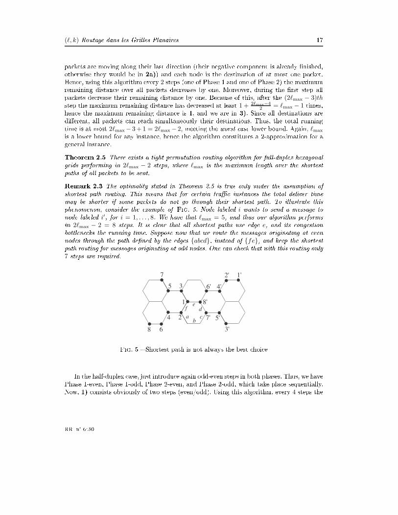
(ℓ, k)-Routage dans les Grilles Planaires 17pa kets are moving along their last dire tion (their negative omponent is already nished,otherwise they would be in 2a)) and ea h node is the destination of at most one pa ket.Hen e, using this algorithm every 2 steps (one of Phase 1 and one of Phase 2) the maximumremaining distan e over all pa kets de reases by one. Moreover, during the rst step allpa kets de rease their remaining distan e by one. Be ause of this, after the (2ℓmax − 3)thstep the maximum remaining distan e has de reased at least 1 + 2ℓmax−42 = ℓmax − 1 times,hen e the maximum remaining distan e is 1, and we are in 3). Sin e all destinations aredierent, all pa kets an rea h simultaneously their destinations. Thus, the total runningtime is at most 2ℓmax − 3 + 1 = 2ℓmax − 2, meeting the worst ase lower bound. Again, ℓmaxis a lower bound for any instan e, hen e the algorithm onstitutes a 2-approximation for ageneral instan e.Theorem 2.5 There exists a tight permutation routing algorithm for full-duplex hexagonalgrids performing in 2ℓmax − 2 steps, where ℓmax is the maximum length over the shortestpaths of all pa kets to be sent.Remark 2.3 The optimality stated in Theorem 2.5 is true only under the assumption ofshortest path routing. This means that for ertain tra instan es the total deliver timemay be shorter if some pa kets do not go through their shortest path. To illustrate thisphenomenon, onsider the example of Fig. 5. Node labeled i wants to send a message tonode labeled i′, for i = 1, . . . , 8. We have that ℓmax = 5, and thus our algorithm performsin 2ℓmax − 2 = 8 steps. It is lear that all shortest paths use edge e, and its ongestionbottlene ks the running time. Suppose now that we route the messages originating at evennodes through the path dened by the edges abcd, instead of fe, and keep the shortestpath routing for messages originating at odd nodes. One an he k that with this routing only
7 steps are required.24
e1
5 3
6
6'
1'2'
3'
4'
5'
8
7
7'
8'd
ba
f
cFig. 5 Shortest path is not always the best hoi eIn the half-duplex ase, just introdu e again odd-even steps in both phases. Thus, we havePhase 1-even, Phase 1-odd, Phase 2-even, and Phase 2-odd, whi h take pla e sequentially.Now, 1) onsists obviously of two steps (even/odd). Using this algorithm, every 4 steps theRR n° 6480
18 Omid Amini , Florian Hu , Ignasi Sau , Janez erovnikmaximum remaining distan e de reases by one. In addition, during the rst 2 steps andduring the last 2 steps all pa kets de rease their remaining distan e by one. Thus, the totalrunning time is at most twi e the time of the full-duplex ase, that is 2(2ℓmax−2) = 4ℓmax−4steps, meeting again the lower bound for the running time of any routing algorithm usingshortest path routing. Again, this algorithm onstitutes a 4-approximation for a generalinstan e.Theorem 2.6 There exists an tight permutation routing algorithm for half-duplex hexagonalgrids performing in 4ℓmax − 4 steps, where ℓmax is the maximum length over the shortestpaths of all pa kets to be sent.Remark 2.4 As explained in Appendix A, there exists an embedding of the triangular gridinto the hexagonal grid with load, dilation, and ongestion 2. Using this embedding, anyalgorithm performing on k steps on the triangular gird performs on 2k steps on the hexagonalgrid. Using this fa t, we obtain a permutation routing algorithm on full-duplex hexagonalgrids performing on 2ℓmax steps. Note that the optimal result given in Theorem 2.5 is slightlybetter.The same applies to half-duplex hexagonal networks, with a running time of 4ℓmax usingthe embedding, in omparison to 4ℓmax − 4 steps given by Theorem 2.6.3 (1, any)-RoutingIn this ase the routing model is the following : ea h pa ket has at most one pa ket tosend, but there are no onstraints on the destination. That is, in the worst ase all pa kets an be sent to one node. This spe ial ase where all pa kets want to send a message to thesame node in often alled gathering in the literature [5. Noti e that this routing model is on eptually dierent from the (1, k)-routing, where the maximum number of pa kets thata node an re eive is xed a priori.Square grid Assume rst that edges are bidire tional. The modi ations for the half-duplex ase are similar to those explained in the previous se tion.We will fo us on the ase where all pa kets surrounding a given vertex want to send apa ket to that vertex. We all this situation entral routing, and if we want to spe ify thatall nodes at distan e at most r from the enter want to send a pa ket, we note it as r- entralrouting. Note that this situation is realisti in many pra ti al appli ations, sin e the entralvertex an play the role of a router or a gateway in a lo al network.Lemma 3.1 (Lower Bound) The number of steps required in a r- entral routing is atleast (
r+12
).Proof: Let us use the bise tion bound [17 to prove the result. It is easy to ount the num-ber of points at distan e at most r from the enter, whi h is 4(
r+12
). Now onsider the ut onsisting of the four edges outgoing from the entral vertex. All pa kets must traverse oneINRIA

(ℓ, k)-Routage dans les Grilles Planaires 19of these edges to arrive to the entral vertex. This ut gives the bise tion bound of 4(
r+12
)
/4routing steps. 2Let us now des ribe an algorithm meeting the lower bound.Proposition 3.1 There exists an optimal r- entral routing algorithm on square grids per-forming in (
r+12
) routing steps.Proof: Express ea h node address in terms of the relative address with respe t to the entral vertex. In this way ea h node is given a label (a, b). Then, for ea h pa ket pla ed ina node with label (a, b) our routing algorithm performs the following :• If ab = 0, send the pa ket along the dire tion of the non-zero omponent.• If ab > 0, send the pa ket along the verti al axis.• If ab < 0, send the pa ket along the horizontal axis.Queues are managed so that the pa kets having greater remaining distan e have priority.This routing divides the square grid into 4 subregions surrounding the entral vertex,as shown in Fig. 6. The type of routing performed in ea h subregion is symbolized by anarrow.
Fig. 6 Division of the grid in the proof of Proposition 3.1Let us now ompute the running time in the r- entral ase. It is obvious that using thisalgorithm all pa kets are sent to the 4 axis outgoing from the entral vertex. The ongestionof the edge in the axis ontaining the entral vertex along ea h line is 1+2+3+. . .+r =(
r+12
).Sin e at ea h step one pa ket rea hes its destination along ea h line, we on lude that (
r+12
)is the total running time of the algorithm. 2Triangular grid The same idea of the square grid applies to the triangular grid. In this ase, the number of nodes at distan e at most r is 6(
r+12
). The ut is made of 6 edges.Dividing the plane onto 6 subregions gives again an optimal algorithm performing in (
r+12
)steps.RR n° 6480
20 Omid Amini , Florian Hu , Ignasi Sau , Janez erovnikHexagonal grid The same idea gives an optimal routing in the r- entral ase. In this ase the degree of ea h vertex is 3, and then it is easy to he k (maybe a drawing usingFig. 3 an help) that there are 3(
r+12
) nodes at distan e at most d that may want to senda message to the entral vertex, and the ut has size 3. As expe ted, the running time isagain (
r+12
).4 (ℓ, k)-RoutingRe all that in the general (ℓ, k)-routing problem ea h node an send at most ℓ pa ketsand re eive at most k pa kets. We propose a distributed approximation algorithm usingthe ideas of the algorithms that we have developed for the permutation routing problem.We also provide lowers bounds for the running time of any algorithm using shortest pathrouting, that allow us to prove that our algorithm is tight when ℓ = k, on any grid.Remark 4.1 We also propose in Appendix B an approa h to nd a solution of the (ℓ, k)-routing problem, on any grid, using the problem of Weighted Edge Coloring in a bi-partite graph. Nevertheless, the algorithm obtained using this approa h is entralized.We start by des ribing the results for full-duplex triangular grids. The results an be ompletely adapted to square grids, but we fo us on the other grids sin e there were fewresults in the literature. We also show how to adapt the results to hexagonal grids and tothe half-duplex version. In this se tion we denote c :=⌈
maxℓ,kminℓ,k
⌉
=⌈
max ℓk , k
ℓ ⌉. Note that
c ≥ 1. Lemma 4.1 and Lemma 4.2 provide two lower bounds for the running time of anyalgorithm using shortest paths.Lemma 4.1 (First lower bound) The worst- ase running time of any algorithm for (ℓ, k)-routing on full-duplex triangular grids using shortest path routing satisesRunning time ≥ minℓ, k · ℓmaxProof: Consider a set of ℓmax nodes pla ed along a line, pla ed onse utively at one sideof a distinguished edge e. Ea h node wants to send minℓ, k messages to the nodes pla edat the other side of e along the line, at distan e ℓmax from it. Then the ongestion of e isminℓ, k · ℓmax, giving the bound. 2Denition 4.1 Given a vertex v, we all the re tangle of side (a, b) starting at v the setRv
a,b = v +αi+βj, 0 ≤ α < a, 0 ≤ β < b We all su h a re tangle a square if a = b. Noti ethat in the triangular grid the node set is generated by i, j,k, where k = −i− j, as we haveexplained in Se tion 2.2.Using standard graph terminology, given a graph G = (V, E) and a subset S ⊆ V , theset Γ(S) denotes the (open) neighborhood in G of the verti es in S. The following theorem an be found, for example, in [13. INRIA

(ℓ, k)-Routage dans les Grilles Planaires 21Theorem 4.1 (Corollary of Hall's theorem [13) Let G = (V, E) be a bipartite graph,with V = X ∪ Y . If for all subsets A of X, |Γ(A)| ≥ c|A|, then for ea h x ∈ X, there existsSx ⊂ Y su h that |Sx| = c, and ∀x, x′ ∈ X, Sx ∩ Sx′ = ∅ and Sx ⊂ Γ(x).We use this theorem to prove the following lower bound.Lemma 4.2 (Se ond lower bound) The worst- ase running time of any algorithm for(ℓ, k)-routing on full-duplex triangular grids using shortest path routing satisesRunning time ≥ ⌈
maxℓ, k4
·⌊
ℓmax + 1√c + 1
⌋⌉
,where c =⌈
maxℓ,kminℓ,k
⌉.Proof: Suppose without loss of generality that ℓ ≥ k, otherwise repla e ℓ by maxℓ, k. Letv be a vertex, and onsider the square Rv
d,d, with d :=⌊
ℓmax+1√c+1
⌋. We laim that all nodesinside this square an send ℓ messages su h that all destination nodes are in the destinationset D = Rvd+ℓmax,d+ℓmax
\Rvd,d. Let S be the subgrid generated by positive linear ombinationsof the ve tors i and j. More pre isely, S := v + αi + βj , α ≥ 0, β ≥ 0. Fig. 2b gives agraphi al illustration.To prove this, we onsider a bipartite graph H on vertex set Rv
d,d ∪ D, with an edgebetween a vertex of Rvd,d and a vertex of D if they are at distan e at most ℓmax in S. Toapply Theorem 4.1, we have to show that any subset of verti es A ⊂ Rv
d,d has at least c|A|neighbors in H . Theorem 4.1 will then ensure the existen e of a feasible repartition of themessages from verti es of Rvd,d to those of D su h that they all travel a distan e at most
ℓmax.Given A ⊂ Rvd,d, let us all DA := u ∈ D : distS(A, u) ≤ ℓmax, where distS(A, u)means the minimum distan e in S from any vertex of A to the vertex u. For any A ⊂ Rv
d,d,we need to show that|DA| ≥ c|A| (1)Without loss of generality we suppose that A is maximal, in the sense that there is noset A′ stri tly ontaining A with DA = DA′ . Instead of onsidering all possible sets A, wewill show below that we an restri t ourselves to re tangles. Hen e given a set A, we denoteby RA the smallest re tangle ontaining the subset of verti es A. We rst laim that
|DRA\ DA| ≤ |RA \ A| (2)Indeed, this equality an be shown by indu tion on |RA\A|. For |RA\A| = 0 the equalityis trivial. Suppose that it is true for |RA \ A|. The indu tion step onsists in showing thatthere is an element x in RA \ A su h that |DRA
\ DA∪x| − |DRA\ DA| ≤ 1 (note thatRR n° 6480

22 Omid Amini , Florian Hu , Ignasi Sau , Janez erovnikDRA∪x = DRA
) :• If there exists x su h that x+ j and x− i are in A and x− j is not in A, then we sele tthis x. From x the only new vertex we may add to DA is x + ℓmaxi.• Otherwise, if there exists x su h that x − j and x − i are in A and x + i is not in A,then we sele t this x. In this ase the only new vertex we may add to DA is x− ℓmaxk.• If none of the previous ases holds, sin e RA is the smallest re tangle ontaining A,and A is maximal, then ne essarily there exists an x su h that x + i and x − j are in
A and x− i is not in A. We sele t this x, and the only new vertex we may add to DAis x + ℓmaxj.Thus, in all ases there exists an x adding at most one neighbor to DRA\DA, whi h nishesthe indu tion step and proves Equation (2). To nish the proof of the fa t that we anrestri t ourselves to re tangles, we show that, for any subset A, if Inequality (1) holds for
RA, then it also holds for A. Indeed, Inequality (1) applied to RA gives :c|RA| ≤ |DRA
| , whi h is equivalent toc(|A| + |RA \ A|) ≤ |DA| + |DRA
\ DA| (3)Using Inequality (2) and the fa t that c ≥ 1, Inequality (3) learly implies that Inequality(1) holds.Hen eforth we assume that A is a re tangle. The last simpli ation onsists in provingthat we an restri t ourselves to re tangles ontaining v. In other words, it will be su ientto prove Inequality (1) for all re tangles Rva,b. Given a re tangle R not positioned at v, there tangle R′ of the same size positioned at v has less neighbors, hen e if Inequality (1) holdsfor R′, it also holds for R.Finally let us prove that Inequality (1) holds for all re tangles Rv
a,b, with 1 ≤ a, b < d.We have that |Rva,b| = ab and |DRv
a,b| = (a + ℓmax)(b + ℓmax) − d2.By the hoi e of d, starting from the Inequality d2 ≤ (ℓmax+1)2
c+1 and using that 1 ≤ a, b,one obtains that d2c ≤ (ℓmax + a)(ℓmax + b) − d2 for any 1 ≤ a, b < d. This implies, usinga, b < d, that cab ≤ (a + ℓmax)(b + ℓmax) − d2 for any 1 ≤ a, b < d, hen e Inequality (1) (i.e.c|Rv
a,b| ≤ |DRva,b
|) holds.So by Theorem 4.1, ea h one of the d2 nodes in Rvd,d an send ℓ messages to the nodes of
D. Sin e the number of edges going from Rvd,d to D is 4d− 1, we apply the bise tion bounddis ussed in Se tion 1.1.1 to on lude that there is an edge of the border of the square Rv
d,dwith ongestion at least ⌈
ℓ·d2
4d−1
⌉
>⌈
ℓ·d4
⌉. This nishes the proof of the lemma. 2We observe that this se ond lower bound is stri tly better than the rst one if and onlyif INRIA

(ℓ, k)-Routage dans les Grilles Planaires 23c√
c + 1>
4ℓmax
ℓmax + 1If both c and ℓmax are big, the ondition be omes approximately :maxℓ, kminℓ, k > 16That is, the se ond lower bound is better when the dieren e between ℓ and k is big.This is the ase of broad ast or gathering, where messages are originated (or destined) from(or to) a small set of nodes of the network.The two lower bounds an be ombined to give :Lemma 4.3 (Combined lower bound) The worst- ase running time of any algorithmfor (ℓ, k)-routing on full-duplex triangular grids using shortest path routing satisesRunning time ≥ max
(
ℓmax · minℓ, k, maxℓ, k ·⌊
ℓmax + 1
4√
c + 1
⌋)
≈ ℓmax·max
(
minℓ, k, maxℓ, k4√
c + 1
)Now we provide an algorithm from whi h we derive an upper bound.Proposition 4.1 (Upper bound (algorithm)) The algorithm for (ℓ, k)-routing on full-duplex triangular grids is the following : route all pa kets as in the permutation routing ase.That is, at ea h node send pa kets rst in their negative omponent, breaking ties arbitrarily(there an be ℓ pa kets in oni t in a negative omponent). If there are no pa kets withnegative omponents, send any of the (at most k) pa kets with maximum remaining distan e.Running time ≤
minℓ, k · c(c−1)2 + maxℓ, k · (ℓmax − c + 1) , if c ≤ ℓmax
minℓ, k · ℓmax(ℓmax+1)2 , if c > ℓmaxProof: Suppose again without loss of generality that ℓ ≥ k. We pro eed by de reasingindu tion on ℓmax. We prove that after minℓ, ℓmaxk steps, ea h paquet will be at distan eat most ℓmax − 1 of its destination. This yieldsRunning time(ℓmax) ≤ minℓ, ℓmaxk + Running time(ℓmax − 1)
≤ minℓ, ℓmaxk +
minℓ, k · c(c−1)2 + maxℓ, k · (ℓmax − c) , if c ≤ ℓmax − 1
minℓ, k · ℓmax(ℓmax−1)2 , if c > ℓmax − 1
≤
minℓ, k · c(c−1)2 + maxℓ, k · (ℓmax − c + 1) , if c ≤ ℓmax
minℓ, k · ℓmax(ℓmax+1)2 , if c > ℓmaxLet us onsider the messages at distan e ℓmax to their destinations. They are of twotypes, the one moving a ording to their negative omponent and the one moving a ordingto their positive omponent.RR n° 6480

24 Omid Amini , Florian Hu , Ignasi Sau , Janez erovnikIf c ≤ ℓmax the rst ones move after at most ℓ time steps. If c < ℓmax they move morequi kly, indeed they move at least on e every ℓmaxk steps (ℓmaxk ≤ c · k = ℓ). This is due tothe fa t that when c < ℓmax at a given vertex, at most ℓmaxk messages may have to movea ording to their negative omponent toward a node at distan e ℓmax.About the messages whi h move a ording to their positive omponent, sin e a node isthe destination of at most k messages, they may wait at most k steps.Consequently, ℓmax de reases by at least one every minℓ, ℓmaxk steps, whi h gives theresult. 2This gives an algorithm whi h is fully distributed. Dividing the running time of thisalgorithm by the ombined lower bound we obtain the following ratio :
minℓ,k·(c
2)+maxℓ,k·(ℓmax−c+1)
ℓmax·max“
minℓ,k ,maxℓ,k4√
c+1
” , if c ≤ ℓmax
minℓ,k·(ℓmax+1)
2·max“
minℓ,k , maxℓ,k4√
c+1
” , if c > ℓmaxWe observe that in all ases the running time of the algorithm is at most maxℓ, k·ℓmax.In parti ular, when ℓ = k (that is, c = 1) the running time is exa tly maxℓ, k · ℓmax =minℓ, k · ℓmax, and therefore it is tight (see lower bound of Lemma 4.1).Corollary 4.1 There exists a tight algorithm for (k, k)-routing in full-duplex triangulargrids.The previous algorithms an be generalized for half-duplex triangular grids as well as forfull and half-duplex hexagonal grids. The generalization to half-duplex grids is obtained byjust adding a fa tor 2 in both the lower bound and the running time of the algorithm, as wedid for the permutation routing algorithm. Thus, let us just fo us on the ase of full-duplexhexagonal grids, for whi h we have the following theorems :Theorem 4.2 There exists an algorithm for (ℓ, k)-routing in full-duplex hexagonal gridswhose running time is at most :Running time ≤
2 minℓ, k · c(c−1)2 + 2 maxℓ, k · (ℓmax − c + 1) , if c ≤ ℓmax
2 minℓ, k · ℓmax(ℓmax+1)2 , if c > ℓmaxLemma 4.4 (First lower bound) No algorithm based on shortest path routing an routeall messages using less than 2 minℓ, k · ℓmax − minℓ, k steps in the worst ase.Denition 4.2 Given a vertex v, we all the re tangle of the hexagonal grid of side (a, b)starting at v to the subset of the hexagonal grid Rv
hexa,b = v + αi + βj + γk, 0 ≤ α <
a,−γ < β < b, 0 ≤ γ < b ∩H where H is the vertex set of the hexagonal grid. We all su ha re tangle a square if a = b.INRIA
(ℓ, k)-Routage dans les Grilles Planaires 25The following lemma gives a se ond lower bound on the running time of any algorithmusing shortest path routing on full-duplex hexagonal grids.Lemma 4.5 (Se ond lower bound) The worst- ase running time of any algorithm usingshortest path routing on full-duplex hexagonal grids satises :Running time ≥ ⌈
maxℓ, k(2d +d − 2
2d + 1)
⌉
,where d =
⌊√73c+64ℓ2max+121+144ℓmax
8√
c+1− 3
8
⌋ and c =⌈
maxℓ,kminℓ,k
⌉.Noti e that when ℓmax
c is big, this value tends to 2 maxℓ, k ℓmax√c+1
, obtaining a perfor-man e around twi e better than in triangular grids.Proof: The proof onsists in showing that the verti es of Rvhexd,d an simultaneously send
max(ℓ, k) messages to some verti es of Rvhexd+ℓmax,d+ℓmax
\ Rvhexd,d. This is done as for thetriangular grid, using again Theorem 4.1. We do not give all the details, sin e the idea behindis the same as the proof of Lemma 4.2.Sin e the number of verti es inside Rv
hexd,d is 4d2 + d − 2, and the number of edgesoutgoing from Rvhexd,d is 2d + 1, the ongestion on these edges is maxℓ, k 4d2+d−2
2d+1 =
maxℓ, k(2d + d−22d+1 ). 25 Con lusions and Further Resear hIn this arti le we have studied the permutation routing, the r- entral routing and thegeneral (ℓ, k)-routing problems on plane grids, that is square grids, triangular grids and hexa-gonal grids. We have assumed the store-and-forward ∆-port model, and onsidered both fulland half-duplex networks. The main new results of this arti le are the following :1. Tight (also in luding the onstant fa tor) permutation routing algorithms on full-duplex hexagonal grids, and half duplex triangular and hexagonal grids.2. Tight (also in luding the onstant fa tor) r- entral routing algorithms on triangularand hexagonal grids.3. Tight (also in luding the onstant fa tor) (k, k)-routing algorithms on square, trian-gular and hexagonal grids.4. Good approximation algorithms for (ℓ, k)-routing in square, triangular and hexagonalgrids, together with new lower bounds on the running time of any algorithm usingshortest path routing.
RR n° 6480

26 Omid Amini , Florian Hu , Ignasi Sau , Janez erovnikAll these algorithms are ompletely distributed, i.e. an be implemented independently atea h node. Finally, we have also formulated the (ℓ, k)-routing problem as aWeighted EdgeColoring problem on bipartite graphs.There still remain several interesting open problems on erning (ℓ, k)-routing on planegrids. Of ourse, the most hallenging problem seems to nd a tight (ℓ, k)-routing algorithmfor any plane grid, for ℓ 6= k. Another interesting avenue for further resear h is to take intoa ount the queue size. That is, to devise (ℓ, k)-routing algorithms with bounded queue size,or that optimize both the running time and the queue size, under a ertain trade-o.A knowledgment. We want to thank Frédéri Giroire, Cláudia Linhares-Sales and Bru eReed for insightful dis ussions.Référen es[1 J. Aspnes, Y. Azar, A. Fiat, S. Plotkin, and O. Waarts. On-line routing of virtual ir uits with appli ations to load balan ing and ma hine s heduling. Journal of theACM (JACM), 44(3) :486504, 1997.[2 J. Aspnes, C. Bus h, S. Dolev, P. Fatourou, C. Georgiou, and A. Shvartsman. EightOpen Problems in Distributed Computing. Bulletin of the EATCS no, 90 :109126,2006.[3 B. Awerbu h and Y. Azar. Lo al optimization of global obje tives : ompetitive distri-buteddeadlo k resolution and resour e allo ation. Foundations of Computer S ien e,1994 Pro eedings., 35th Annual Symposium on, pages 240249, 1994.[4 Y. Azar, E. Cohen, A. Fiat, H. Kaplan, and H. Rä ke. Optimal oblivious routing inpolynomial time. Journal of Computer and System S ien es, 69(3) :383394, 2004.[5 J.-C. Bermond, J. Galtier, R. Klasing, N. Morales, and S. Pérennes. Hardness andapproximation of Gathering in stati radio networks. Parallel Pro essing Letters,16(2) :165183, 2006.[6 A. Borodin and J. Hop roft. Routing, merging and sorting on parallel models of ompu-tation. Pro eedings of the fourteenth annual ACM symposium on Theory of omputing,pages 338344, 1982.[7 C. Bus h, M. Magdon-Ismail, and J. Xi. Oblivious routing on geometri networks.Pro eedings of the 17th annual ACM symposium on Parallelism in algorithms and ar- hite tures, pages 316324, 2005.[8 C. Bus h, M. Magdon-Ismail, and J. Xi. Optimal oblivious path sele tion on the mesh.Pro eedings of the International Parallel and Distributed Pro essing Symposium (IPDPS2005), Denver, Colorado, USA, April, 2005. INRIA
(ℓ, k)-Routage dans les Grilles Planaires 27[9 J. Cogolludo and S. Rajasekaran. Permutation Routing on Re ongurable Meshes.Algorithmi a, 31 :4457, 2001.[10 A. Datta. A Fault-Tolerant Proto ol for Energy-E ient Permutation Routing in Wi-reless Networks. IEEE Transa tions on Computers, 54(11) :14091421, November 2005.[11 D. de Werra, M. Demange, B. Es oer, J. Monnot, and V. T. Pas hos. Weighted Colo-ring on Planar, Bipartite and Split Graphs : Complexity and Improved Approximation.Le ture Notes in Computer S ien e, 3341 :896907, 2004.[12 M. Demange, D. de Werra, J. Monnot, and V. T. Pas hos. Weighted node oloring :when stable sets are expensive. WG'02 LNCS, 2573 :114125, 2002.[13 R. Diestel. Graph Theory. Springer-Verlag, 2005.[14 T. Dobrave , B. Robi£, and J. erovnik. Permutation routing in double-loop networks :design and empiri al evaluation. Journal of Systems Ar hite ture, 48 :387402, 2003.[15 T. Dobrave , J. erovnik, and B. Robi£. An optimal message routing algorithm for ir ulant networks. Journal of Systems Ar hite ture, 52 :298306, 2006.[16 P. Fraigniaud and E. Lazard. Methods and problems of ommuni ation in usual net-works. Dis rete Applied Mathemati s, 53 :79134, 1994.[17 M. D. Grammatikakis, M. K. D. F. Hsu, and J. Sibeyn. Pa ket Routing in Fixed-Conne tion Networks : a Survey. Journal of Parallel and Distributed Pro essing,54(2) :77132, 1998.[18 J. T. Havill. Online Pa ket Routing on Linear Arrays and Rings. Le ture Notes inComputer S ien e, 2076 :773784, 2001.[19 F. Hwang, T. Lin, and R. Jan. A Permutation Routing Algorithm for Double LoopNetwork. Parallel Pro essing Letters, 7(3) :259265, 1997.[20 F. Hwang, Y. Yao, and B. Dasgupta. Some permutation routing algorithms for low-dimensional hyper ubes. Theoreti al Computer S ien e, 270 :111124, 2002.[21 G. E. Jan and M.-B. Lin. Con entration, load balan ing, partial permutation rou-ting, and super on entration on ube- onne ted y les parallel omputers. Journal ofParallel and Distributed Compututing, 65 :14711482, 2005.[22 C. Kaklamanis, D. Krizan , and T. Tsantilas. Tight bounds for oblivious routing in thehyper ube. Theory of Computing Systems, 24(1) :223232, 1991.[23 D. Karimou and J. F. Myoupo. An Appli ation of an Initialization Proto ol to Permuta-tion Routing in a Single-Hop Mobile Ad Ho Networks. The Journal of Super omputing,RR n° 6480

28 Omid Amini , Florian Hu , Ignasi Sau , Janez erovnik31 :215226, 2005.[24 A. Kesselman and K. Kogan. Non-Preemptive S heduling of Opti al Swit hes. In IEEEGLOBECOM, pages 18401844, 2004.[25 S. Klavºar, A. Vesel, and P. igert. On resonan e graphs of ata ondensed hexagonalgraphs : stru ture, oding, and hamiltonian path algorithm. MATCH Communi ationsin Mathemati al and in Computer Chemistry, 49(49) :99116, 2003.[26 E. Kranakis, H. Sing, and J. Urrutia. Compas Routing in Geometri Graphs. In 11thCanadian Conferen e of Computational Geometry, pages 5154, 1999.[27 M. Kunde, R. Niedermeier, and P. Rossmanith. Faster sorting and routing on grids withdiagonals. In 11th Symposium of Theoreti al Computer S ien e, 775, pages 225236.Le ture Notes on Computer S ien e, 1994.[28 F. Leighton, B. M. Maggs, and A. W. Ri ha. Fast Algorithms for Finding O(Congestion+ Dilation) Pa ket Routing S hedules. In 28th Annual Hawaii International Conferen eon System S ien es, pages 555563, 1995.[29 F. T. Leighton, B. M. Maggs, and S. B. Rao. Pa ket Routing and Job-Shop S hedulingin O( ongestion + dilation) Steps. Combinatori a, 14(2) :167186, 1994.[30 T. Leighton. Introdu tion to Parallel Algorithms and Ar hite tures : Arrays-Trees-Hyper ubes. Morgan-Kaufman, San Mateo, California, 1992.[31 T. Leighton, B. Maggs, and S. Rao. Universal pa ket routing algorithms. Foundationsof Computer S ien e, 1988., 29th Annual Symposium on, pages 256269, 1988.[32 T. Leighton, F. Makedon, and I. G. Tollis. A 2n− 2 Step Algorithm for Routing in ann × n Array with Constant-Size Queues. Algorithmi a, 14 :291304, 1995.[33 W. Liang and X. Shen. Permutation Routing in All-Opti al Produ t Networks. IEEETransa tions on Cir uits and Systems, 49(4) :533538, 2002.[34 B. Maggs. A Survey of Congestion+ Dilation Results for Pa ket S heduling. 40thAnnual Conferen e on Information S ien es and Systems, 22(24) :15051510, 2006.[35 B. Maggs, F. auf der Heide, B. Vo king, and M. Westermann. Exploiting lo ality fordata management in systems of limited bandwidth. Pro eedings of the 38th AnnualIEEE Symposium on Foundations of Computer S ien e, pages 284293, 1997.[36 F. Makedon and A. Symvonis. Optimal algorithms for the many-to-one routing problemon 2-dimensional meshes. Mi ropro essors and Mi rosystems, 17 :361367, 1993.[37 F. G. No etti, I. Stojmenovi¢, and J. Zhang. Addressing and Routing in Hexagonal
INRIA

(ℓ, k)-Routage dans les Grilles Planaires 29Networks with Appli ations for Tra king Mobile Users and Conne tion Rerouting inCellular Networks. IEEE Transa tions on Parallel and Distributed Systems, 13(9) :963971, 2002.[38 R. Ostrovsky and Y. Rabani. Universal O( ongestion + dilation + log1+ε N) Lo alControl Pa ket Swit hing Algorithms. In 29th Annual ACM Symposium on the Theoryof Computing, pages 644653, New York, 1997.[39 A. Pietra aprina and G. Pu i. Optimal Many-to-One Routing on the Mesh withConstant Queues. Le ture Notes in Computer S ien e, 2150 :645649, 2001.[40 H. Ra ke. Minimizing ongestion in general networks. Foundations of ComputerS ien e, 2002. Pro eedings. The 43rd Annual IEEE Symposium on, pages 4352, 2002.[41 S. Rajasekaran and R. Overholt. Constant queue routing on a mesh. Journal of Paralleland Distributed Computing, 15 :160166, 1992.[42 B. Robi£ and J. erovnik. Minimum 2-terminal routing in 2-jump ir ulant graphs.Computers and Arti ial Intelligen e, 19(1) :3746, 2000.[43 I. Sau and J. erovnik. An Optimal Permutation Routing Algorithm for Full-DuplexHexagonal Mesh Networks. Preprint series, University of Ljubljana, Institute of Ma-themati s, Physi s and Me hani s, 44(1017), 2006. ISSN 13184865.[44 I. Sau and J. erovnik. Optimal permutation routing on mesh networks. In Pro . ofInternational Network Optimization Conferen e, Belgium, April 2007. 6 pages.[45 C. S heideler. Universal Routing Strategies for Inter onne tion Networks. Springer,1998.[46 J. Sibeyn. Routing on Triangles, Tori and Honey ombs. International Journal of Fun-dations of Computer S ien e, 8(3) :269287, 1997.[47 J. Sibeyn and M. Kaufman. Deterministi 1-k routing on meshes (with appli ationsto worm-hole routing). In LNCS, editor, 11th Symposium on Theoreti al Aspe ts ofComputer S ien e, volume 775, pages 237248, 1994.[48 J. F. Sibeyn, B. S. Chlebus, and M. Kaufmann. Deterministi Permutation Routing onMeshes. Journal of Algorithms, 22(1) :111141, 1997.[49 A. Srinivasan and C.-P. Teo. A onstant-fa tor approximation algorithm for pa ketrouting, and balan ing lo al vs. global riteria. In STOC '97 : Pro eedings of thetwenty-ninth annual ACM symposium on Theory of omputing, pages 636643, NewYork, NY, USA, 1997. ACM.[50 I. Stojmenovi¢. Honey omb Networks : Topologi al Properties and Communi ationRR n° 6480

30 Omid Amini , Florian Hu , Ignasi Sau , Janez erovnikAlgorithms. IEEE Transa tions on Parallel and Distributed Systems, 8(10) :10361042,1997.[51 T. Suel. Routing and Sorting on Meshes with Row and Column Buses. In ParallelPro essing Symposium, volume Eighth International Volume, pages 411417, 1994.[52 R. To²i¢, D. Masulovi¢, I. Stojmenovi¢, J. Brunvoll, B. Cyvin, and S. Cyvin. Enume-ration of Polyhex Hydro arbons up to h=17. Journal of Chemi al Information andComputer S ien es, 35 :181187, 1995.[53 R. Trobe . Two-dimensional regular d-meshes. Parallel Computing, 26 :19451953,2000.[54 L. Valiant and G. Brebner. Universal s hemes for parallel ommuni ation. Pro eedingsof the thirteenth annual ACM symposium on Theory of omputing, pages 263277, 1981.[55 R. Williams. The Geometri al Foundation of Natural Stru ture : A Sour e Book ofDesign. Dover Publi ations, 1979.
INRIA
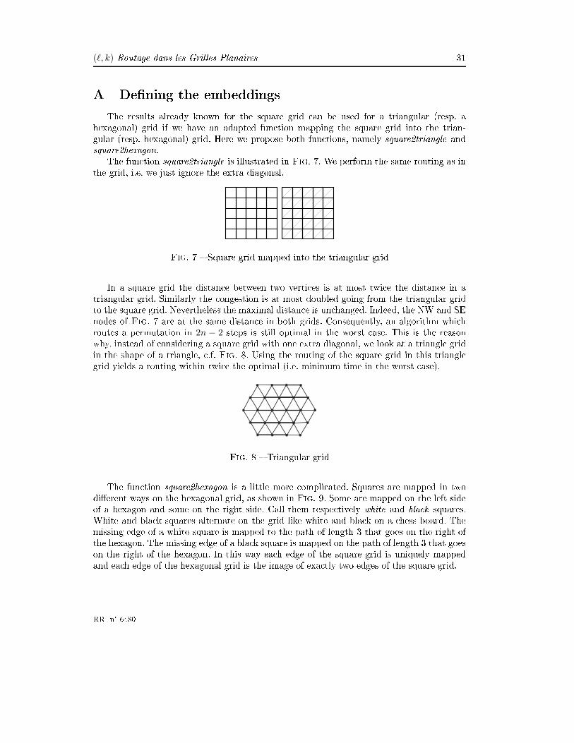
(ℓ, k)-Routage dans les Grilles Planaires 31A Dening the embeddingsThe results already known for the square grid an be used for a triangular (resp. ahexagonal) grid if we have an adapted fun tion mapping the square grid into the trian-gular (resp. hexagonal) grid. Here we propose both fun tions, namely square2triangle andsquare2hexagon.The fun tion square2triangle is illustrated in Fig. 7. We perform the same routing as inthe grid, i.e. we just ignore the extra diagonal.Fig. 7 Square grid mapped into the triangular gridIn a square grid the distan e between two verti es is at most twi e the distan e in atriangular grid. Similarly the ongestion is at most doubled going from the triangular gridto the square grid. Nevertheless the maximal distan e is un hanged. Indeed, the NW and SEnodes of Fig. 7 are at the same distan e in both grids. Consequently, an algorithm whi hroutes a permutation in 2n − 2 steps is still optimal in the worst ase. This is the reasonwhy, instead of onsidering a square grid with one extra diagonal, we look at a triangle gridin the shape of a triangle, .f. Fig. 8. Using the routing of the square grid in this trianglegrid yields a routing within twi e the optimal (i.e. minimum time in the worst ase).
Fig. 8 Triangular gridThe fun tion square2hexagon is a little more ompli ated. Squares are mapped in twodierent ways on the hexagonal grid, as shown in Fig. 9. Some are mapped on the left sideof a hexagon and some on the right side. Call them respe tively white and bla k squares.White and bla k squares alternate on the grid like white and bla k on a hess board. Themissing edge of a white square is mapped to the path of length 3 that goes on the right ofthe hexagon. The missing edge of a bla k square is mapped on the path of length 3 that goeson the right of the hexagon. In this way ea h edge of the square grid is uniquely mappedand ea h edge of the hexagonal grid is the image of exa tly two edges of the square grid.RR n° 6480
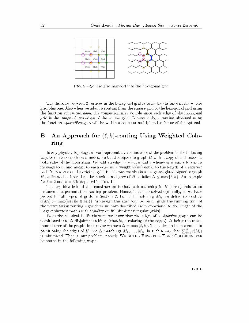
32 Omid Amini , Florian Hu , Ignasi Sau , Janez erovnikWhite
WhiteWhite
WhiteWhite
Black Black
Black
Black
Fig. 9 Square grid mapped into the hexagonal gridThe distan e between 2 verti es in the hexagonal grid is twi e the distan e in the squaregrid plus one. Also when we adapt a routing from the square grid to the hexagonal grid usingthe fun tion square2hexagon, the ongestion may double sin e ea h edge of the hexagonalgrid is the image of two edges of the square grid. Consequently, a routing obtained usingthe fun tion square2hexagon will be within a onstant multipli ative fa tor of the optimal.B An Approa h for (ℓ, k)-routing Using Weighted Colo-ringIn any physi al topology, we an represent a given instan e of the problem in the followingway. Given a network on n nodes, we build a bipartite graph H with a opy of ea h node atboth sides of the bipartition. We add an edge between u and v whenever u wants to send amessage to v, and assign to ea h edge uv a weight w(uv) equal to the length of a shortestpath from u to v on the original grid. In this way we obtain an edge-weighted bipartite graphH on 2n nodes. Note that the maximum degree of H satises ∆ ≤ maxℓ, k. An examplefor ℓ = 2 and k = 3 is depi ted in Fig. 10.The key idea behind this onstru tion is that ea h mat hing in H orresponds to aninstan e of a permutation routing problem. Hen e, it an be solved optimally, as we haveproved for all types of grids in Se tion 2. For ea h mat hing Mi, we dene its ost asc(Mi) := maxw(e)|e ∈ Mi). We assign this ost be ause on all grids the running time ofthe permutation routing algorithms we have des ribed are proportional to the length of thelongest shortest path (with equality on full-duplex triangular grids).From the lassi al Hall's theorem we know that the edges of a bipartite graph an bepartitioned into ∆ disjoint mat hings (that is, a oloring of the edges), ∆ being the maxi-mum degree of the graph. In our ase we have ∆ = maxℓ, k. Thus, the problem onsists inpartitioning the edges of H into ∆ mat hings M1, . . . , M∆, in su h a way that ∑∆
i=1 c(Mi)is minimized. That is, our problem, namely Weighted Bipartite Edge Coloring, anbe stated in the following way :INRIA

(ℓ, k)-Routage dans les Grilles Planaires 33l=2 k=3
u
v
w(uv)
Fig. 10 Bipartite graph modeling a (2, 3)-routing instan eWeighted Bipartite Edge ColoringInput : An edge-weighted bipartite graph H .Output :A partition of the edges ofH into mat hingsM1, . . . , M∆, with c(Mi) := maxw(e)|e ∈Mi).Obje tive : min
∑∆i=1 c(Mi).Therefore, min
∑∆i=1 c(Mi) is the running time for routing an (ℓ, k)-routing instan e usingthis algorithm.Unfortunately, in [11Weighted Edge Coloring is proved to be stronglyNP- ompletefor bipartite graphs, whi h is the ase we are interested in. In fa t, the problem remainsstrongly NP- omplete even restri ted to ubi and planar bipartite graphs. Con erning ap-proximation results, the authors [11 provide an inapproximability bound of 7
6 − ε, for anyε > 0. Furthermore, they mat h this bound with an approximation algorithm within 7/6 ongraphs with maximum degree 3, improving the best known approximation ratio of 5/3 [12.In [24 this innaproximability bound is proved independently on general bipartite graphs.Thus, if maxℓ, k ≤ 3 we an nd a solution of Weighted Bipartite Edge Coloringwithin 7
6 times the optimal solution, and this will be also a solution for the (ℓ, k)-routingproblem.Remark B.1 Although of theoreti al value, the main problem of this algorithm is that n-ding these mat hings is a entralized task. In addition, the true ratio, i.e. related to theoptimum of the (ℓ, k)-routing, should be proved to provide an upper bound for the runningtime of this algorithm.RR n° 6480

Unité de recherche INRIA Sophia Antipolis2004, route des Lucioles - BP 93 - 06902 Sophia Antipolis Cedex (France)
Unité de recherche INRIA Futurs : Parc Club Orsay Université- ZAC des Vignes4, rue Jacques Monod - 91893 ORSAY Cedex (France)
Unité de recherche INRIA Lorraine : LORIA, Technopôle de Nancy-Brabois - Campus scientifique615, rue du Jardin Botanique - BP 101 - 54602 Villers-lès-Nancy Cedex (France)
Unité de recherche INRIA Rennes : IRISA, Campus universitaire de Beaulieu - 35042 Rennes Cedex (France)Unité de recherche INRIA Rhône-Alpes : 655, avenue de l’Europe - 38334 Montbonnot Saint-Ismier (France)
Unité de recherche INRIA Rocquencourt : Domaine de Voluceau- Rocquencourt - BP 105 - 78153 Le Chesnay Cedex (France)
ÉditeurINRIA - Domaine de Voluceau - Rocquencourt, BP 105 - 78153 Le Chesnay Cedex (France)http://www.inria.fr
ISSN 0249-6399

Improper colouring of weighted grid and hexagonal
graphs
Jean-Claude Bermond∗ Frederic Havet ∗ Florian Huc ∗ and C. Linhares †
November 21, 2008
1 Introduction
This paper is motivated by a problem posed by Alcatel Space Technologies (see [1]). A satellite sendsinformations to receivers on earth, each of which is listening several frequencies, one for each signalit needs to receive. Technically it is impossible to focus a signal sent by the satellite exactly on thedestination receiver. So part of the signal is spread in an area around it creating noise for the otherreceivers displayed in this area and listening the same frequency. Each receiver is able to distinguish thesignal directed to it from the extraneous noises it picks up if the sum of the noises does not become toobig, i.e. does not exceed a certain threshold T . The problem is to assign frequencies to the receivers insuch a way that each receiver gets its dedicated signals properly, while minimizing the total number offrequencies used.
Generally the ”noise relation” is symmetric, that is if a receiver u is in the noise area of a receiver vthen v is in the noise area of u. Hence, interferences may be modelled by a noise graph G = (V (G), E(G))which vertices are the receivers and in which two vertices are joined by an edge if and only if they interfer.Moreover, the graph is attached a weight function p : V (G) → IN, where the weight p(v) of the vertexv is equal to the number of signals it has to receive. Hence we have a weighted graph, that is a pair(G, p) where G is a graph and p a weight function on the vertex set of G. The weight function can beintuitively extended to sets of vertices and to subgraphs: the weight of a set of vertices S ⊂ V (G) isp(S) =
∑
v∈S p(v) while the weight of a subgraph H ⊂ G is p(H) = p(V (H)). The maximum weight of avertex in a graph (G, p) is denoted pmax.
In a simplified version, the intensity I of the noise created by a signal is independent of the frequencyand the receiver. Hence to distinguish its signal from noises, a receiver must be in the noise area of at mostk =
⌊
TI
⌋
receivers listening signals on the same frequency. Hence the problem come to find a colouringof the weighted graph which is k-improper. Let (G, p) be a weighted graph. A colouring of (G, p) is afunction C : V → P(S) such that |C(v)| ≥ p(v). The set S is called the set of colours and is usually1, 2, . . . , l for some integer l as we are only interested in its cardinality. A weighted colouring into a setS of cardinality l is called an l-colouring of (G, p). A weighted colouring C of (G, p) is k-improper if forany colour i, the set of vertices coloured i induces a graph of degree at most k. The k-improper chromaticnumber of (G, p), denoted χk(G, p), is the smallest l such that (G, p) admits a k-improper l-colouring.Note that a 0-improper colouring corresponds to a proper colouring.
∗Projet Mascotte I3S (CNRS & UNSA) and INRIA, INRIA Sophia-Antipolis, 2004 route des Lucioles, BP 93, 06902Sophia-Antipolis Cedex. E-mail: (bermond|fhavet|fhuc)@sophia.inria.fr. Partially supported by the european projectFET-AEOLUS.
†Universidade Federal do Ceara, Departamento de Computacao, Bloco 910, Campus do Pici, Fortaleza, Ceara, CEP60455-760, Brasil. [email protected]
1

In [1] this problem is studied via linear programming. The objective of this paper is to build algorithmsgiving k-improper colouring of weighted graphs of a certain class C with as few colours as possible. Analgorithm that gives a k-improper colouring of each weighted graph (G, p) ∈ C with at most c1×χk(G, p)+c2 colours for some constants c1 and c2, is said to be c1-approximate or to have approximation ratio c1.
Let q be an integer. We denote by q the constant weight function equal to q. A natural methodto find a k-improper colouring of (G, p) consists in finding first a k-improper colouring of (G,q) with rcolours, ideally χk(G,q), and then in dividing each weight into sets of size q; using r colours for each
of these sets, we obtain a k-improper r ×⌈
pmax
q
⌉
-colouring of (G, p). As χk(G, p) ≥ pmax, it gives an
(r/q)-approximate algorithm.
Proposition 1 Given a colouring C of (G,q) with r colours, there is an easy polynomial algorithm that
colours (G, p) with at most r⌈
pmax
q
⌉
colours.
In particular, χk(G,q) ≤ r, then χk(G, p) ≤ r⌈
pmax
q
⌉
.
In this paper, we present improvements of this proposition. For any graph G, we denote ρk(H, G, p),or simply ρk(H) when (G, p) is clear from the context, the maximum of χk(H ′, p) over the subgraphsH ′ of G isomorphic to H . For example, ρk(K1) = pmax and ρ0(K2) = maxp(u) + p(v) | uv ∈ E(G)and ρk(K2) = pmax if k ≥ 2. By extension, if H is a family of graphs (finite or not), ρk(H, G, p) is themaximum of ρk(H, G, p) over all graphs H ∈ H. Obviously, for any family H, ρk(H, G, p) ≤ χk(G, p).The idea to design approximate algorithms for k-improper colouring is to find a finite family of graphsHk such that any weighted graph (G, p) in the considered class satisfies χk(G, p) ≤ c1.ρk(Hk) + c2 withc1 a small constant (ideally 1) and c2 another constant. Hence computing χk(H ′, p) for all the subgraphsH ′ isomorphic to a graph in Hk, we obtain a c1-approximate algorithm for χk(G, p). Moreover we alsoexhibit algorithms that produce the corresponding c1-approximate k-improper colouring.
We first show approximate algorithms for general graphs. We then make further improvements forspecific graphs, namely the grid graphs and the hexagonal graphs. The next subsections recall the resultsknown for grid graphs and hexagonal graphs.
1.1 Grid graphs
The (two-dimensionnal) grid is the graph GL defined as follows: the vertices are all integer linear com-binations af1 + bf2 of the two vectors f1 = (1, 0) and f2 = (0, 1): thus we may identify the vertices withthe pairs (a, b) of integers. Two vertices are adjacent when the Euclidean distance between them is 1.Thus each vertex x = (a, b) has four neighbours: its left neighbour (a− 1, b), its right neighbour (a+1, b),its top neighbour (a, b + 1) and its down neighbour (a, b− 1). A grid graph is an induced subgraph of thetwo-dimensionnal grid.
(a+1,b)
(a,b−1)
(a−1,b)
(a,b+1)e2
e1
Figure 1: The two-dimensionnal grid and a grid graph.
As a grid graph G has maximum degree 4, for k ≥ 4, k-improper colouring of G are trivial : giving any
2
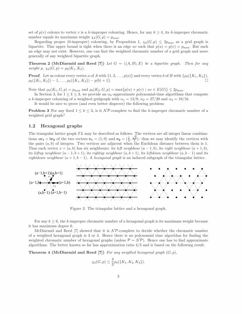
set of p(v) colours to vertex v is a k-improper colouring. Hence, for any k ≥ 4, its k-improper chromaticnumber equals its maximum weight χk(G, p) = pmax.
Regarding proper (0-improper) colouring, by Proposition 1, χ0(G, p) ≤ 2pmax as a grid graph isbipartite. This upper bound is tight when there is an edge uv such that p(u) = p(v) = pmax. But suchan edge may not exist. However, one can find the weighted chromatic number of a grid graph and moregenerally of any weighted bipartite graph.
Theorem 2 (McDiarmid and Reed [7]) Let G = ((A, B), E) be a bipartite graph. Then for anyweight p, χ0(G, p) = ρ0(K1, K2).
Proof. Let us colour every vertex a of A with 1, 2, . . . , p(a) and every vertex b of B with ρ0(K1, K2),ρ0(K1, K2) − 1, . . . , ρ0(K1, K2) − p(b) + 1.
Note that ρ0(K1, G, p) = pmax and ρ0(K2, G, p) = maxp(u) + p(v) | uv ∈ E(G) ≤ 2pmax.In Section 3, for 1 ≤ k ≤ 3, we provide an αk-approximate polynomial-time algorithms that compute
a k-improper colouring of a weighted gridgraph with α1 = 13/9, α2 = 27/20 and α3 = 19/16.It would be nice to prove (and even better disprove) the following problem:
Problem 3 For any fixed 1 ≤ k ≤ 3, is it NP-complete to find the k-improper chromatic number of aweighted grid graph?
1.2 Hexagonal graphs
The triangular lattice graph TL may be described as follows. The vertices are all integer linear combina-
tions ae1 + be2 of the two vectors e1 = (1, 0) and e2 = (12 ,
√3
2 ): thus we may identify the vertices withthe pairs (a, b) of integers. Two vertices are adjacent when the Euclidean distance between them is 1.Thus each vertex x = (a, b) has six neighbours: its left neighbour (a − 1, b), its right neighbour (a + 1, b),its leftup neighbour (a− 1, b + 1), its rightup neighbour (a, b + 1), its leftdown neighbour (a, b − 1) and itsrightdown neighbour (a + 1, b − 1). A hexagonal graph is an induced subgraph of the triangular lattice.
(a+1,b)
(a−1,b+1)(a,b+1)
(a−1,b)
(a+1,b−1)(a,b−1)
e1
e2
Figure 2: The triangular lattice and a hexagonal graph.
For any k ≥ 6, the k-improper chromatic number of a hexagonal graph is its maximum weight becauseit has maximum degree 6.
McDiarmid and Reed [7] showed that it is NP-complete to decide whether the chromatic numberof a weighted hexagonal graph is 3 or 4. Hence there is no polynomial time algorithm for finding theweighted chromatic number of hexagonal graphs (unless P = NP). Hence one has to find approximatealgorithms. The better known so far has approximation ratio 4/3 and is based on the following result.
Theorem 4 (McDiarmid and Reed [7]) For any weigthed hexagonal graph (G, p),
χ0(G, p) ≤4
3ρ0(K1, K2, K3).
3
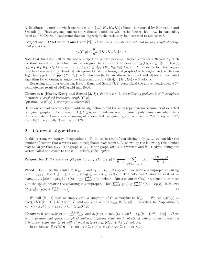
A distributed algorithm which guarantees the 43ρ0(K1, K2, K3) bound is reported by Narayanan and
Schende [6]. However, one expects approximate algorithms with ratios better than 4/3. In particular,Reed and McDiarmid conjecture that for big weight the ratio may be decreased to almost 9/8.
Conjecture 5 (McDiarmid ans Reed [7]) There exists a constant c such that for any weigthed hexag-onal graph (G, p),
χ0(G, p) ≤9
8ρ0(K1, K2, K3) + c.
Note that the ratio 9/8 in the above conjecture is best possible. Indeed consider a 9-cycle C9 withconstant weight k. A colour can be assigned to at most 4 vertices, so χ0(C9, k) ≥ 9k
4 . Clearly,ρ0(K1, K2, K3, C9, k) = 2k. So χ0(C9, k) ≥ 9
8ρ0(K1, K2, K3, C9, k). An evidence for this conjec-ture has been given by Havet [2] who proved that if a hexagonal graph G is triangle-free (i.e. has noK3) then χ0(G, p) ≤ 7
6ρ0(K1, K2) + 5. See also [9] for an alternative proof and [4] for a distributedalgorithm for colouring triangle-free hexagonal graph with 5
4ρ0(K1, K2) + 3 colours.Regarding improper colouring, Havet, Kang and Sereni [3, 8] generalized the above mentionned NP-
completeness result of McDiarmid and Reed:
Theorem 6 (Havet, Kang and Sereni [3, 8]) For 0 ≤ k ≤ 5, the following problem is NP-complete:Instance: a weighted hexagonal graph (G, p).Question: is (G, p) k-improper 3-colourable?
Hence one cannot expect polynomial-time algorithm to find the k-improper chromatic number of weightedhexagonal graphs. In Section 4, for 1 ≤ k ≤ 5, we provide an αk-approximate polynomial-time algorithmsthat compute a k-improper colouring of a weighted hexagonal graph with α1 = 20/11, α2 = 12/7,α3 = 18/13, α4 = 80/63 and α5 = 41/36.
2 General algorithms
In this section, we improve Proposition 1. To do so, instead of considering only pmax, we consider thenumber of colours that a vertex and its neighbours may require. As shown by the following, this numbermay be larger than pmax. The graph K1,k+1 is the graph with k + 2 vertices and k + 1 edges linking onevertex, called the centre to the k + 1 others, called spikes.
Proposition 7 For every weight function p, χk(K1,k+1, p) ≥1
k + 1
∑
v∈V (K1,k+1)
p(v) =p(K1,k+1)
k + 1.
Proof. Let u be the centre of K1,k+1 and v1, . . . , vk+1 its spikes. Consider a k-improper colouringC of K1,k+1. For 1 ≤ i ≤ k + 1, set q(vi) = |C(vi) \ C(u)|. The colouring C uses at least M =
max1≤i≤k+1q(vi) + p(u) ≥ p(u) + 1k+1
∑k+1i=1 q(vi) colours. But a colour in C(u) is assigned to at most
k of the spikes because the colouring is k-improper. Thus∑k+1
i=1 q(vi) ≥∑k+1
i=1 p(vi) − kp(u). It follows
M ≥ 1k+1
(
p(u) +∑k+1
i=1 p(vi))
.
We call (k + 1)-star, or simply star, a subgraph of G isomorphic to K1,k+1. We set θk(G, p) =maxp(H)/(k + 1) | H star of G and ωk(G, p) = maxpmax, θk(G, p). According to Proposition 7,ωk(G, p) ≤ ρ(K1, K1,k+1, G, p) ≤ χk(G, p).
Theorem 8 Let αk(r, q) = (k+1)r2
(k+2)rq−q2 and βk(r, q) = max(k + 2)r2 − rq, (k + 1)r2 + krq. There
is a algorithm that given a graph G and a k-improper colouring C of (G,q) with r colours, returns ak-improper colouring (G, p) with at most αk(r, q) × ωk(G, p) + βk(r, q) colours.
In particular, if χk(G,q) ≤ r, then χk(G, p) ≤ αk(r, q) × ωk(G, p) + βk(r, q).
4

Proof. Consider the following algorithm :
Algorithm 1 0. Initialisation: (G0, p0) := (G, p), S := ∅ and i = 0.
1. Add the vertices of low weight to S that will be treated at the end (Step 3):Si := v ∈ V (G) | pi(v) ≤ γk(r, q) with γk(r, q) = q
rβk(r, q), S := S ∪ Si and for all v ∈ Si,
s(v) := pi(v). Gi+1 := Gi − Si.
2. If Gi+1 is not empty:
2.1. Give to each vertex v of Gi+1 a certain number ni(v) of colours among a set of (k + 1)r2
colours in such a way that ωk(Gi+1, pi − ni) ≤ ωk(Gi, pi) − (k + 2)rq + q2.
2.2. Set pi+1 := pi − ni and i := i + 1 and go to Step 1.
3. Colour (G〈S〉, s) with βk(r, q) colours. It is possible using γk(r, q)/q times the colouring C assmax ≤ γk(r, q).
At each Step 2, (k + 1)r2 colours are used and ωk decreases by at least (k + 2)rq − q2. Therefore,
Algorithm 1 yields a k-improper colouring of (G, p) with at most (k+1)r2
(k+2)rq−q2 ωk(G, p) + βk(r, q) colours.
Let us now describe precisely how to perform Step 2.1. Set ωk = ωk(Gi, pi). A big star is a star H ofGi+1 such that pi(H) ≥ (k + 1)ωk − q2 and a big vertex is a vertex such that pi(v) > ωk − rq. A smallvertex is a non-big vertex. It is goofy if it is adjacent to a big vertex and regular otherwise.
Set a = (k + 1)r − q. At each step 2.1, we first use a times the colouring C : with ar colours, eachvertex receives aq of them. Then we use rq additional colours: they are all assigned to big vertices andregular vertices receive q2 (using q times C on regular vertices). Hence ni(v) = (k + 2)rq − q2 if v is big,ni(v) = (k + 1)rq if v is regular and ni(v) = (k + 1)rq − q2 if v is goofy.
Notice that in Gi+1, no star is made of k + 2 big vertices. Consequently the previous colouring isindeed k-improper.
Let us now check that ωk(Gi+1, pi+1) ≤ ωk − (k + 2)rq + q2.We have pi+1
max ≤ ωk − (k + 2)rq + q2 : indeed for a vertex v, pi+1(v) ≤ pi(v) − ni(v). If v is bigni(v) = (k + 2)rq − q2 and if v is small ni(v) ≥ (k + 1)rq − q2 and pi(v) ≤ ωk − rq. In both cases,pi+1(v) ≤ ωk − (k + 2)rq + q2.
Consider now a star H of Gi+1. Each vertex receives at least qa colours. Hence if H is not big,
pi+1(H) ≤ pi(H) − (k + 2)qa ≤ (k + 1)ωk − q2 − (k + 2)qa = (k + 1)(ωk − (k + 2)rq + q2).
Suppose now that H is big.
Claim 1 H has a vertex x which is not goofy.
Proof. Let u be the centre of H and v1, . . . , vk+1 its spikes with pi(v1) ≥ · · · ≥ pi(vk+1). Suppose for acontradiction that all the vertices of H are goofy. Then there exists a big vertex v0 adjacent to u. Thevertex v0 is not one of the vi for these are small. Let H ′ be the star with centre u and spikes v0, . . . , vk.Set S =
∑k
j=1 pi(vj). We have pi(H ′) = pi(u) + S + pi(v0) ≤ (k + 1)ωk and pi(v0) > ωk − rq. Hence
S < kωk + rq − pi(u). But pi(vk+1) ≤Sk
so pi(vk+1) < ωk + rq
k− pi(u)
k.
Now pi(H) = pi(u)+S +pi(vk+1) so by the above inequalities, pi(H) < (k+1)ωk +rq(k+1k
)−pi(u)/k.As u ∈ Gi+1, we have pi(u) ≥ γk(r, q) ≥ (k + 1)rq + kq2, thus pi(H) < (k + 1)ωk − q2. This contradictsthe fact that H is big.
5

The vertex x receives at least qa + q2 colours. Hence
pi+1(H) ≤ pi(H) − (k + 2)qa − q2 ≤ (k + 1)ωk − (k + 2)qa − q2 ≤ (k + 1)(ωk − (k + 2)rq + q2).
Thus θk(Gi+1, pi+1) ≤ ωk − (k + 2)rq + q2, so ωk(Gi+1, pi+1) ≤ ωk − (k + 2)rq + q2.
Algorithm 1 requires to compute the value of ωk(G, p). Since there are at most n(
∆k+1
)
k + 1-stars in
a graph on n vertices with maximum degree ∆, it can be done in O(
n(
∆k+1
)
)
operations.
For 1-improper colouring or when the maximum degree ∆ of the graph G is k + 1, one can get betterapproximate algorithms. They are very similar to Algorithm 1 but one can improve Claim 1 and thusTheorem 8.
Theorem 9 Let r and q be two integers. Set a = 2r − 2q if r ≥ 2q and a = r if r ≤ 2q, and α′1(r, q) =
ar+rqaq+rq
and β′1(r, q) = 4r2. There is a polynomial algorithm that given a weighted graph G and a 1-
improper colouring C of (G,q) with r colours, produces a 1-improper colouring of (G, p) with at mostα′
1(r, q) × ωk(G, p) + β′1(r, q) colours.
In particular, if χ1(G,q) ≤ r, then χ1(G, p) ≤ α′1(r, q) × ω1(G, p) + β′
1(r, q).
Proof. Consider the following algorithm :
Algorithm 2 0. Initialisation: (G0, p0) := (G, p), S := ∅ and i = 0.
1. Add the vertices of low weight to S that will be treated at the end (Step 3):Si := v ∈ V (G) | pi(v) ≤ 4rq, S := S ∪ Si and for all v ∈ Si, s(v) := pi(v). Gi+1 := Gi − Si.
2. If Gi+1 is not empty:
2.1. Give to each vertex v of Gi+1 a certain number ni(v) of colours among a set of ar + rq coloursin such a way that ω1(G
i+1, pi − ni) ≤ ω1(Gi, pi) − aq − rq.
2.2. Set pi+1 := pi − ni and i := i + 1 and go to Step 1.
3. Colour (G〈S〉, s) with 4r2 colours. It is possible using 4r times the colouring C as smax ≤ 4rq.
Algorithm 2 yields a 1-improper colouring of (G, p) with at most α′1ω1(G, p) + β′
1 colours.
Let us now describe precisely how to perform Step 2.1. Set ω1 = ω1(Gi, pi). As before, a big vertex
is a vertex such that pi(v) > ω1 − rq. A small vertex is a non-big vertex. It is goofy if it is adjacent to abig vertex and regular otherwise. A 2-star H is big if pi(H) > 2ω1 − 2rq.
At each step 2.1, we first use a times the colouring C : with ar colours, each vertex receives aq ofthem. Then we use rq additional colours: they are all assigned to big and regular vertices receive q2 ofthem (using q times C on regular vertices). Hence ni(v) = aq + rq if v is big, ni(v) = aq + q2 if v isregular and ni(v) = aq if v is goofy.
Let us now check that ω1(Gi+1, pi+1) ≤ ω1 − aq − rq.
We have pi+1max ≤ ω1−aq−rq : indeed for a vertex v, pi+1(v) ≤ pi(v)−ni(v). If v is big ni(v) = aq+rq
and if v is small ni(v) ≥ aq et pi(v) ≤ ω1 − rq. In both cases, pi+1(v) ≤ ω1 − aq − rq.Consider a 2-star H of Gi+1. Each vertex receives at least qa colours. Hence if H is not big then
pi+1(H) ≤ pi(H) − 3aq ≤ 2ω1 − 2rq − arq.Suppose now that H is big.
Claim 2 A 2-star with two goofy vertices and no big vertex is not big.
6
Proof. Suppose H is a 2-star with centre u2 and spikes u1 and u3 and assume that two vertices aregoofy and none is big. W.l.o.g. there is a big vertex b1 adjacent to u1 and a big vertex b2 adjacent tou2 or u3. As b1, u1 and u2 form a K1,2, by definition of ω1,
12 (pi(b1) + pi(u1) + pi(u2)) ≤ ω1. Similarly,
12 (pi(b2) + pi(u2) + pi(u3)) ≤ ω1. Hence pi(u1) + pi(u2) + pi(u3) ≤ 4ω1 − pi(b1) − pi(b2) − pi(u2) ≤2ω1 − pi(u2) + 2rq − 2. As u2 is in Gi+1, pi(u2) ≥ 4rq − 2, so pi(H) ≤ 2ω1 − 2rq.
So H contains a big vertex or two regular ones. Hence pi+1(H) ≤ pi(H) − 3qa − minrq, 2q2. By ourchoice of a, we get pi+1(H) ≤ 2(ω1 − aq − rq).
Theorem 10 Let r and q be two integers. Set a = (k + 1)r − 2 if r ≥ 2q and a = kr if r ≤ 2q, andα′′
k(r, q) = ar+rqaq+rq
and β′′k (r, q) = ar + r2. There exists a polynomial algorithm that given a graph G with
maximum degree k + 1 and a k-improper colouring C of (G,q) with r colours, produces a k-impropercolouring of (G, p) with at most α′′
k(r, q) × ωk(G, p) + β′′k (r, q) colours.
In particular, if χk(G,q) ≤ r, then χk(G, p) ≤ α′′k(r, q) × ωk(G, p) + β′′
k (r, q).
Proof. Consider the following algorithm :
Algorithm 3 0. Initialisation: (G0, p0) := (G, p), (S, s) is the empty graph and i = 0.
1. Add the vertices of low weight to S that will be treated at the end (Step 3):Si := v ∈ V (G) | pi(v) ≤ aq + rq, S := S ∪ Si and for all v ∈ Si, s(v) := pi(v). Gi+1 := Gi − Si.
2. If Gi+1 is not empty:
2.1. Give to each vertex v of Gi+1 a certain number ni(v) of colours among a set of (a+ q)r coloursin such a way that ωk(Gi+1, pi − ni) ≤ ωk(Gi, pi) − aq − rq.
2.2. Set pi+1 := pi − ni and i := i + 1 and go to Step 1.
3. Colour (G〈S〉, s) with β′′k colours. It is possible using a+r times the colouring C as smax ≤ (a+r)q.
Algorithm 3 yields a k-improper colouring of (G, p) with at most α′′kωk(G, p) + β′′
k colours.
Let us now describe precisely how to perform Step 2.1. Set ωk = ωk(Gi, pi). A big vertex is a vertexsuch that pi(v) > ωk − rq. A small vertex is a non-big vertex. It is goofy if it is adjacent to a big vertexand regular otherwise. A regular vertex is isolated if it is adjacent to no regular vertex.
At each step 2.1, we first use a times the colouring C : with ar colours, each vertex receives aqof them. Then we use rq additional colours: they are all assigned to big and isolated regular verticesand non-isolated regular vertices receive q2 (using q times C on non-isolated regular vertices). Henceni(v) = aq + rq if v is big or isolated regular, ni(v) = aq + q2 if v is non-isolated regular and ni(v) = aqif v is goofy.
Let us now check that ωk(Gi+1, pi+1) ≤ ωk − aq − rq.We have pi+1
max ≤ ωk−aq−rq : indeed for a vertex v, pi+1(v) ≤ pi(v)−ni(v). If v is big ni(v) = aq+rqand if v is small ni(v) ≥ aq et pi(v) ≤ ωk − rq. In both cases, pi+1(v) ≤ ωk − aq − rq.
Consider a star H of Gi+1. Each vertex receives at least aq colours.
Claim 3 A star H contains a big vertex or an isolated regular vertex x or two non-isolated regularvertices.
7

Proof. Let u be the centre of H and v1, . . . , vk+1 its spikes. Since G has maximum degree k + 1 theonly neighbours of u are the vi. Hence, if no vertex of H is big then u is regular. Moreover if it is notisolated one of the vi is also regular.
Hence H contains a vertex that receives at least aq + rq colours or two vertices receiving at least aq + q2
colours. Hence pi+1(H) ≤ pi(H) − (k + 2)qa − minrq, 2q2. By our choice of a, we get pi+1(H) ≤(k + 1)(ωk − aq − rq). Thus θk(Gi+1, pi+1) ≤ ωk − aq − rq, so ωk(Gi+1, pi+1) ≤ ωk − aq − rq.
3 Grid graphs
3.1 General algorithms applied to grid graphs
In order to apply Theorems 8 and 10 to grid graphs, we determine χk(GL,q) for every positive integerq and 1 ≤ k ≤ 3.
We first prove a preliminary lemma. Let C be a colouring of a weighted graph (G, p). We denote bycu,v the number of colours assigned to both u and v, that is cu,v = |C(u) ∩ C(v)|. We use the standardnotation N(u) for the neighborhood of u.
Lemma 11 Let C be a k-improper colouring of a weighted graph (G, p).
(i)∑
v∈N(u)
cu,v ≤ kp(u);
(ii) ∀u, v, C uses at least p(u) + p(v) − cu,v colours;
(iii) ∀u, v, w, C uses at least p(u) + p(v) + p(w) − cu,v − cu,w − cv,w.
Proof. (i) A colour assigned to u is assigned to at most k neighbours of u because C is k-improper.(ii) and (iii) follow from the Inclusion-Exclusion Formula:
|C(u) ∪ C(v)| = |C(u)| + |C(v)| − |C(u) ∩ C(v)| = p(u) + p(v) − cu,v;
|C(u) ∪ C(v) ∪ C(w)| = |C(u)| + |C(v)| + |C(w)| − |C(u) ∩ C(v)| − |C(u) ∩ C(w)| − |C(v) ∩ C(w)|
+|C(u) ∩ C(v) ∩ C(w)|
≥ p(u) + p(v) + p(w) − cu,v − cu,w − cv,w.
Theorem 12 For the grid graph GL, we have:
(i) χ1(GL,q) = 2q,
(ii) χ2(GL,q) =⌈
3q
2
⌉
, and
(iii) χ3(GL,q) =⌈
5q4
⌉
.
8

1,3 1,2
1,3 1,21,3 1,2
1,2 1,2 1,3 1,22,3 1,3
2,3 1,3 1,2 1,3 1,2
1,3 1,2 1,3 1,2 1,3
1,2 1,3 1,22,3
2,3 2,3 2,3
2,3
2,3
2,3
2,3
2,3
2,3
Figure 3: A 2-improper colouring of the square grid.
Proof. Let us first show the k-improper colourings of (GL,q) with the required number of colours.(i) The grid is bipartite so (GL,q) has a 0-improper (and thus also 1-improper) colouring with 2q
colours.(ii) For 1 ≤ j ≤ 3, let Uj = (a, b) | a + b = j mod 3. Assign the colours
⌈
(j−1)q2
⌉
+ 1, . . . ,⌈
jq
2
⌉
to
vertices which are not in Uj . See Figure 3.(iii) For 1 ≤ j ≤ 5, let Tj be the set of vertices obtained from the vertex (0, j) by adding the linear
combinations of the vectors 2f1 + f2 and 5f1. For 1 ≤ j ≤ 5, assign the colours⌈
(j−1)q4
⌉
+ 1, . . . ,⌈
jq
4
⌉
to
vertices not in Tj. See Figure 4.
1,2,3,4 2,3,4,5 1,3,4,5 1,2,4,5 1,2,3,5 1,2,3,4 2,3,4,5
2,3,4,5 1,3,4,5 1,2,4,5
2,3,4,5 1,3,4,5 1,2,3,51,2,4,5 1,2,3,4 2,3,4,5
1,2,3,51,2,3,41,2,4,5 1,2,3,5
1,2,3,5 2,3,4,5 1,3,4,5 1,2,4,5 1,2,3,41,2,3,5
1,3,4,5 1,2,4,5
1,2,3,4
1,2,3,5 1,2,3,4 2,3,4,5 1,3,4,5 1,2,4,5
1,3,4,5
Figure 4: A 3-improper colouring of the square grid.
Let us now show that these colourings are optimal. Hence let C be a k-improper colouring of (GL,q)with χk(GL,q) colours.
(i) If k = 1, consider a 4-cycle in GL. A colour may be used on at most 2 of these vertices. Hence 2qcolours are needed.
(ii) and (iii) Let u be a vertex of GL. Applying Lemma 11 (ii) to the four neighbours of a vertex u,we obtain: 4χk(GL,q) ≥ 8q −
∑
v∈N(u) cu,v. Now by Lemma 11 (i), 4χk(GL,q) ≥ (8 − k)q. We obtain
respectively χ2(GL,q) ≥ 3q2 and χ3(GL,q) ≥ 5q
4 .
Corollary 13 For 1 ≤ k ≤ 3, there are αk-approximate algorithms for finding a k-improper colouring ofa weighted grid graph, where α1 = 3
2 , α2 = 2720 , and α3 = 19
16 .
Proof. Theorems 9 and 12 give the result for k = 1. Theorems 8 and 12 give the result for k = 2.Theorems 10 and 12 give the result for k = 3.
The following theorem improves this last result for 1-improper colouring of weighted grid graphs:
9

Theorem 14 There is a 3927 -approximate algorithm for finding a 1-improper colouring of weighted grid
graph.
Proof. The idea of the algorithm is still similar but this time we use more the position of big verticesand quasi-big vertices (a new type of vertex to be described) to 1-improper colour the grid graph (cfLemma 4).
Algorithm 4 0. Initialisation: (G0, p0) := (G, p), S := ∅ and i = 0.
1. Add the vertices of low weight to S that will be treated at the end (Step 3):Si := v ∈ V (G) | pi(v) < pinf with pinf = 133, S := S ∪ Si and for all v ∈ Si, s(v) := pi(v).Gi+1 := Gi − Si.
2. If Gi+1 is not empty:
2.1. Give to each vertex v of Gi+1 a certain number ni(v) of colours among a set of 156 colours insuch a way that ωk(Gi+1, pi − ni) ≤ ωk(Gi, pi) − 108.
2.2. Set pi+1 := pi − ni and i := i + 1 and go to Step 1.
3. Colour (G〈S〉, s) with 266 colours. It is possible using as smax ≤ pinf − 1 and χ1(GL, q) = 2q.
Algorithm 4 yields a 1-improper colouring of (G, p) with at most 156108ωk(G, p) + 266 colours.
Let us now describe precisely how to perform Step 2.1. Set ω1 = ω1(Gi, pi). A big vertex is a vertex
such that pi(v) > ω1 − d1 with d1 = 24. A small vertex v is a non-big vertex. It is goofy if it is adjacentto a big vertex (we note Goof the set of goofy vertices), it is quasi-big if pi(v) > ω1 − d2 with d2 = 67and regular otherwise. A 2-star is big if its weight is bigger than 2ω1 − d3 with d3 = 45.
Claim 4 Let u and v be two vertices which are big or quasi-big in Gi. In Gi+1, they are at distance atleast 3 or form a connected component.
Proof. Suppose that u and v are at distance at most 2. If they do not form a connected component inGi+1, there is a vertex w ∈ V (Gi+1) such that the subgraph induced by u, v and w is a 2-star. Hencepi(u) + pi(v) + pi(w) ≤ 2ω1. But pi(u) + pi(v) + pi(w) > 2ω1 − 2d2 + 1 + pinf = 2ω1, a contradiction.Thus u and v form a connected component.
Set a = 48, b = 6 and c = 3. At each step 2.1, we give all the 2a + 8b + 4c colours to the vertices inconnected component of order 2.
For the vertices not in such small components, we use three different colourings. The two first arebased on the following eight sets of vertices:
• U1 = (0, 0) + 2kf1 + k′(f1 − 2f2), (0, 1) + 2kf1 + k′(f1 − 2f2),
• U2 = (1, 0) + 2kf1 + k′(f1 − 2f2), (1, 1) + 2kf1 + k′(f1 − 2f2),
• U3 = (0, 1) + 2kf1 + k′(f1 − 2f2), (0, 2) + 2kf1 + k′(f1 − 2f2),
• U4 = (1, 1) + 2kf1 + k′(f1 − 2f2), (1, 2) + 2kf1 + k′(f1 − 2f2),
• U5 = (0, 0) + 2kf2 + k′(2f1 − f2), (1, 0) + 2kf2 + k′(2f1 − f2),
• U6 = (0, 1) + 2kf2 + k′(2f1 − f2), (1, 1) + 2kf2 + k′(2f1 − f2),
• U7 = (1, 0) + 2kf2 + k′(2f1 − f2), (2, 0) + 2kf2 + k′(2f1 − f2),
10

Figure 5: The sets U1 up to U8.
• U8 = (1, 1) + 2kf2 + k′(2f1 − f2), (2, 1) + 2kf2 + k′(2f1 − f2).
We first assign 2a colours such that each vertex of U1 receive a colours and each vertex of U2 receivesa other colours. Since U1 and U2 form a partition of V , each vertex receives a colours, and since G〈U1〉and G〈U2〉 have maximum degree 1, the colouring we obtain is 1-improper.
Then we use 8b colours denoted by (i, j), 1 ≤ i ≤ b, 1 ≤ j ≤ 8. We give all the colours to the bigvertices. Then, for 1 ≤ j ≤ 8, we give to each vertex of Uj \ Goof the colours (i, j), 1 ≤ i ≤ b. A vertexappears in four of the Uj, so each non-goofy vertex receives 4b colours. Finally, by Claim 4, a goofyvertex u has a unique big neigbour v. There is an integer j such that both u and v are in Uj . We assignto u the colours (i, j), 1 ≤ i ≤ b. Doing so, each goofy vertex receives b colours.
Finally we use 4 sets of c colours At, Ad, Al and Ar. Each big or quasi-big vertex receive the colourof all these sets and each top (resp. down, left, right) receives the colour of At (resp. Ad, Al and Ar).This is 1-improper by Claim 4.
Let us now check that ω1(Gi+1, pi+1) ≤ ω1 − 108.
Let v be a vertex. If it is big then ni(v) = a + 8b + 4c; if it is quasi-big then ni(v) = a + 4b + 4c; if itis goofy then ni(v) = a + b + c; if it is regular then ni(v) ≥ a + 4b and if in addition it is adjacent to aquasi-big vertex ni(v) ≥ a + 4b + c. Hence, by our choice of a, b, c d1 and d2 we have
pi+1max ≤ ω1 − mina + 8b + 4c, d1 + a + 4b + 4c, d2 + a + b + c, d2 + a + 4b ≤ pi
max − 108. (1)
Claim 5 Let H be a big 2-star in (Gi+1, pi). Then the following hold:
(i) if the centre of H is goofy then H has a big vertex;
(ii) if H has two goofy vertices then the third one is big;
(iii) if H has a goofy vertex then it has a big or quasi-big vertex.
Proof. Let v be the centre of H and u1 and u2 its spike.(i) Suppose that v is goofy. Let w be its big neighbour. Suppose for a contradiction that w /∈ u1, u2.
Considering the two 2-stars with vertex sets w, v, u1 and w, v, u2, we obtain that pi(u1) + pi(v) ≤2ω1 − pi(w) ≤ ω1 + d1 − 1 and pi(u2) + pi(v) ≤ 2ω1 − pi(w) ≤ ω1 + d1 − 1. Hence 2ω1 + 2d1 − 2 ≥pi(u1) + pi(u2) + 2pi(v) ≥ pi(v) + pi(H) ≥ pi(v) + 2ω1 − d3 + 1, so pi(v) ≤ 2d1 + d3 − 3, but then v is inSi, which is a contradiction.
(ii) Suppose for a contradiction that H has two goofy vertices and no big vertex. By (i), u1 andu2 are the goofy vertices. Let w1 (resp. w2) be the big neighbour of u1 (resp. u2). (We may have
11

w1 = w2). As in (i), considering the two 2-stars with vertex sets w1, u1, v and w2, u2, v, we obtainpi(u1) + pi(v) ≤ ω1 + d1 − 1 and pi(u2) + pi(v) ≤ ω1 + d1 − 1. These inequalities yield the contradictionas in (i).
(iii) If v is goofy then H has a big vertex by (i). Suppose now that one spike of H , say u1, isgoofy. Let w be the big neighbour of u1. If w = v, we have the result. Assume now that w 6= v.Considering the 2-star induced by w, u1, v, we obtain pi(u1) + pi(v) ≤ ω1 + d1 − 1. Since H is bigpi(u1) + pi(v) + pi(u2) ≥ 2ω1 − d3 + 1. So pi(u2) ≥ ω1 − d1 − d3 + 2, that is u2 is quasi-big.
Let H be a 2-star. If it is not big, its weigth decreases by at least 3a + 3b + 3c. If H is big then byClaim 5, it has either three non-goofy vertices, in which case its weight decreases by at least 3a + 12b,one big vertex and two goofy vertices, in which case its weight decreases by 3a+10b+6c, one big vertex,one regular vertex and one goofy vertex, in which case its weight decreases by 3a + 13b + 5c or onequasi-big vertex, one regular vertex adjacent to this quasi-big and one goofy vertex in which case itsweight decreases by 3a + 9b + 6c. Hence by our choice of a, b, c, for a big star H ,
pi+1(H) ≤ ω1 − min(3a + 12b, 3a + 9b + 6c, 3a + 13b + 5c) ≤ pi(H) − 216. (2)
For Equations (1) and (2) yield ω1(Gi+1, pi+1) ≤ ω1 − 108.
4 Hexagonal graphs
4.1 General algorithms applied to hexagonal graphs
Theorem 15 For the triangular lattice TL, we have:
(i) χ1(TL,q) =⌈
5q2
⌉
,
(ii) χ2(TL,q) = 2q,
(iii) χ3(TL,q) =⌈
3q
2
⌉
,
(iv) χ4(TL,q) =⌈
4q
3
⌉
and
(v) χ5(TL,q) =⌈
7q
6
⌉
.
Proof. Let us first show the k-improper colourings of (TL,q) with the required number of colours.(i) For 1 ≤ j ≤ 5, let Aj be the set of vertices obtained from the vertex (0, j) by adding the linear
combinations of the vectors 2e1 + e2 et 5e1. For 1 ≤ j ≤ 5, assign the colours⌈
(j−1)q2
⌉
+ 1, . . . ,⌈
jq
2
⌉
to
vertices of Aj ∪ Aj+1 (with A6 = A1).(ii) Colour a vertex (a, b) with 1, . . . , q if a is even and with q + 1, . . . , 2q otherwise.(iii) For 1 ≤ j ≤ 3, let Sj be the set of vertices obtained from the vertex (0, j) by adding the linear
combinations of the vectors e1 + e2 et 3e1. Assign the colours⌈
(j−1)q2
⌉
+ 1, . . . ,⌈
jq
2
⌉
to vertices which
are not in Sj .(iv) For 0 ≤ j1 ≤ 1 and 1 ≤ j2 ≤ 2, Tj1+j2 = (a, b) | a ≡ j1 mod 2 et b ≡ j2 mod 2. Assign the
colours⌈
(j−1)q3
⌉
+ 1, . . . ,⌈
jq3
⌉
to vertices which are not in Tj .
(v) For 1 ≤ j ≤ 7, let Uj be the set of vertices obtained from the vertex (0, j) by adding the linear
combinations of the vectors e1 + 2e2 et 7e1. Assign the colours⌈
(j−1)q6
⌉
+ 1, . . . ,⌈
jq6
⌉
to vertices which
are not in Uj .
12

1,25,14,53,41,25,1 2,3
1,25,14,53,41,25,1 2,3
1,2 4,52,33,4 3,45,14,5
1,2 4,52,33,4 3,45,14,5
1,25,14,53,41,25,1 2,3
Figure 6: A 1-improper colouring of the triangular lattice.
Let us now show that these colourings are optimal. Hence let C be a k-improper colouring of (TL,q)with χk(TL,q) colours.
Let u be a vertex of TL. Applying Lemma 11 (i) and (ii) to a vertex u of TL and its six neighbours, weobtain: 6χk(TL,q) ≥ (12−k)q. For k = 3, 4 or 5, we obtain respectively χ3(TL,q) ≥ 3q
2 , χ4(TL,q) ≥ 4q
3
and χ5(TL,q) ≥ 7q6 .
For k = 1 and 2, we need an extra argument. Let u and v be two adjacent vertices and t and w theirtwo common neighbours. Set f(u, v) = cu,t + cu,v + cu,w.
Consider now the ordered pair (u, v) which minimizes f(u, v), i.e. f(u, v) = fmin . Then f(v, u) =cv,t + cu,v + cv,w. So f(u, v) + f(v, u) = (cu,t + cu,v + cv,t) + (cu,w + cu,v + cv,w). By Lemma 11 (iii), wehave f(u, v) + f(v, u) ≥ 6q − 2χk(TL,q).
Let u′ be the vertex symmetrical to u compared to v. By Lemma 11 (i), f(v, u) + f(v, u′) ≤ kq, sof(v, u′) ≤ kq − f(v, u) ≤ kq − 6q + 2χk(TL,q) + fmin.
For k = 1, if χk(TL,q) < 5q2 , we would have f(v, u′) < fmin. Similarly, for k = 2, if χk(TL,q) < 2q,
we would have f(v, u′) < fmin. In both cases, it contradicts the minimality of f in (u, v).
To prove the optimality of the colouring proposed for k = 1 and k = 2, one can also use Lemma 16.Indeed this Lemma says that for k = 1 for every two vertices of a given colour, there is at least threevertices that do not have this colour. For k = 2, it says that for every ℓ vertices of a given colour thereis at least ℓ vertices that do not have this colour.
Lemma 16 Let P be a path in the triangular lattice made of ℓ vertices such that any vertex of P isadjacent to atmost 2 vertices of P . P has exactly ℓ + 1 leftdown and rightdown neighbours.
Let C be a cycle in the triangular lattice made of ℓ vertices such that any vertex of C is adjacent toexactly 2 vertices of C. C has exactly ℓ leftdown and rightdown neighbours.
Proof. We prove both assertions by induction: P(ℓ): ”Let P be a path in the triangular lattice made ofℓ vertices, such that any vertex of P is adjacent to atmost 2 vertices of P . P has exactly ℓ + 1 leftdownand rightdown neighbours.”
P(1) is true.Let ℓ ≥ 2, P(ℓ) ⇒ P(ℓ + 1): Let v be one of the two end verices of P . P \ v has ℓ vertices, so by
P(ℓ), it has ℓ+1 leftdown and rightdown neighbours. According to the 6 positions of v in respect to P asdepicted on Figure 4, one can see that P has exactly one more leftdown and rightdown neighbour thanP \ v. (Either v is leftdown or rightdown neighbour of P \ v and has two neighbours which weren’tleftdown or rightdown neighbour of P \ v or it is not and v brings one new leftdown or rightdownneighbour. In the figures, we use the following code: there is six pairs of grids, in each pairs, the left gridcorrespond to P and the right grid to P \ v. v is represented in full purple, it’s only neighbour in fullred. The common neighbours of P and P \ v are in dashed empty red cycles while the different onesare in empty purple cycles.)
13

P P’
v
v
v v
v
v
Figure 7: The 6 possible positions of an end vertex of P .
P ′(ℓ): ”Let C be a cycle in the triangular lattice made of ℓ vertices, such that any vertex of C isadjacent to exactly 2 vertices of C. c has exactly ℓ leftdown and rightdown neighbours.”
P ′(3) and P ′(6) are true.Let ℓ ≥ 7, ∀ℓ′ ≤ ℓ,P ′(ℓ′) ⇒ P ′(ℓ + 1):Let C be a cycle made of ℓ vertices so that each vertex of C is adjacent to exactly two vertices of C
if such cycle exists. We distinguish two cases according to the structures of the interior of C.C divides the nodes into two connected subsets, we call interior the finite one and denote it by IC .The first case is when there is a vertex v ∈ IC wich is connected to the rest of IC by exactly one
leftdown, left, rightup or right vertex. We consider the cycle C′ wich has IC \ v as interior. C′ has lessthan ℓ vertices so we can apply the induction. According to the position of v the result follow, as shownon Figure 5. In this figure, the vertices of C are full cycles, the leftdown and rightdown neighbours arethe empty cycles. Given a pair of grids, on the left is represented the cycle C, on the right the reducedcycle. The vertices of the cycles and the neighbours that change are in purple, the other in red. Noticethat there is as many extra full purple cycles as there is extra empty purple cycle in the left grid than inthe right one. This number is exactly the number of full line empty cycles.
If there is no such v, we consider a subset of vertices V ⊂ IC with no upright and upleft neighbourssuch that they form a maximal right-left line. We let C′ be the cycle with interior IC \ V . It satisfiesthat each vertex of C′ is adjacent to exactly two vertices of C′ and C′ has less than ℓ − 1 vertices so wecan apply the induction. All possible situations are illustrated on Figure 6.
Remark 17 Note that the above proofs work also for hexagonal graphs containing a sufficiently largehexagonal graphs. For the first proof, for k ≥ 3 it suffices that the graph contains a vertex of degree 6.
14

v
v
v
v
Figure 8: The 4 possible positions for v.
For k = 1, 2, it must contain all the vertices at distance at most kq2 of a given node u : starting from u
and decreasing f at most kq
2 times, yields the desired contradiction. For the proof using Lemma 16, italso works, but one needs a bigger subgrid.
Corollary 18 For 1 ≤ k ≤ 5, there are αk-approximate algorithms for finding a k-improper colouring ofa weighted hexagonal graph, where α1 = 20
11 , α2 = 127 , α3 = 18
13 , α4 = 8063 , and α5 = 41
36 .
Proof. Theorems 9 and 15 give the result for k = 1. Theorems 8 and 15 give the result for 2 ≤ k ≤ 4.Theorems 10 and 15 give the result for k = 5.
5 Conclusion
We have proposed several approximate algorithms whose approximation ratios are summarized in thefollowing table:
Grid Hexagonalk = 1 13/9 20/11k = 2 27/20 12/7k = 3 19/16 18/13k = 4 X 80/63k = 5 X 41/36
It remains to answer Problem 3, ie to find wether or not optimally improper colouring a weighted gridgraph is NP-complete or not.
References
[1] S. Alouf, E. Altman, J. Galtier, J.-F. Lalande, et C. Touati, Quasi-optimal bandwidth allocation formulti-spot MFTDMA satellites, in Proc. IEEE INFOCOM 2005, Miami, FL, 2005.
[2] F. Havet. Channel assignement and multicolouring of the induced subgraphs of the triangular lattice.Discrete Mathematics, 233:219–231, 2001.
15
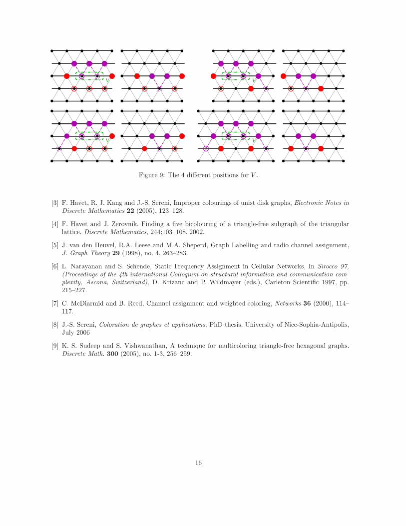
V
V V
V
Figure 9: The 4 different positions for V .
[3] F. Havet, R. J. Kang and J.-S. Sereni, Improper colourings of unist disk graphs, Electronic Notes inDiscrete Mathematics 22 (2005), 123–128.
[4] F. Havet and J. Zerovnik. Finding a five bicolouring of a triangle-free subgraph of the triangularlattice. Discrete Mathematics, 244:103–108, 2002.
[5] J. van den Heuvel, R.A. Leese and M.A. Sheperd, Graph Labelling and radio channel assignment,J. Graph Theory 29 (1998), no. 4, 263–283.
[6] L. Narayanan and S. Schende, Static Frequency Assignment in Cellular Networks, In Sirocco 97,(Proceedings of the 4th international Colloqium on structural information and communication com-plexity, Ascona, Switzerland), D. Krizanc and P. Wildmayer (eds.), Carleton Scientific 1997, pp.215–227.
[7] C. McDiarmid and B. Reed, Channel assignment and weighted coloring, Networks 36 (2000), 114–117.
[8] J.-S. Sereni, Coloration de graphes et applications, PhD thesis, University of Nice-Sophia-Antipolis,July 2006
[9] K. S. Sudeep and S. Vishwanathan, A technique for multicoloring triangle-free hexagonal graphs.Discrete Math. 300 (2005), no. 1-3, 256–259.
16
The Proportional Colouring Problem:Optimising Buffers in Radio Mesh Networks 1
Florian Huc 2
Project team Mascotte - I3S (CNRS-UNS)/INRIA Sophia Antipolis, France
Claudia Linhares-Sales 3
Universidade Federal do Ceara, Brazil
Herve Rivano
Project team Mascotte - I3S (CNRS-UNS)/INRIA Sophia Antipolis, France
Abstract
In this paper, we consider a new edge colouring problem modelling call schedulingoptimisation issues in wireless mesh networks: the proportional edge-colouring. Itconsists in finding a minimum cost edge-colouring of a graph which preserves theproportion given by the weights associated to each of its edges. We show thatdeciding if a weighted graph admits a proportional colouring is polynomial whiledetermining its proportional chromatic index is NP-hard. We then give lower andupper bounds for this parameter that can be computed in polynomial time. Wefinally identify a class of graphs and a class of weighted graphs for which the pro-portional chromatic index can be determined exactly.
Keywords: edge colouring, proportional colouring, mesh networks, call scheduling.

1 Introduction
Wireless mesh networks (WMNs) are cost-effective solutions for ubiquitoushigh-speed services [1]. They are self-organised networks with a fixed infras-tructure of wireless mesh routers interconnected to provide Internet accessto mobile network users. This infrastructure, forming a wireless backhaulnetwork, is connected to Internet by special routers called mesh gateways asdepicted in Figure 1.
Fig. 1. A WMN topology: mobile clients access Internet through a multi-hopwireless backhaul network of routers and gateways.
The fixed infrastructure of the WMN is often modelled by a directed graphG = (V, E) of N nodes representing mesh points. Each device has a singleinterface allowing to send or receive packets on the only channel available.This channel is therefore shared between all the nodes [2]. In the following,the network is assumed to be synchronous. We focus on the steady state ofthe network, which is therefore periodic with a period duration T . The com-munication protocol is a slotted TDMA multiplexing. Computing an optimalallocation of the slots to the links taking radio interference into account refersto the throughput provided to each router. This throughput corresponds tothe ratio of the volume of data sent during a period over T , the duration ofthe period [3].
In the following, we assume that these ratio are given in order to achieve the
1 This work has been partially funded by European project IST/FET AEOLUS and Frenchproject ANR-JC OSERA and ARC CARMA.2 Contact author. Email: [email protected]. F. Huc is supported by CNRSand Region PACA.3 This work has been done while C. Linhares-Sales was visiting the Mascotte project-teamwith support by CNPq/Brazil.

throughput requirements defined by a set of Constant Bit Rate requests. Themain optimisation issue is to find an achievable scheduling of the links, thatis an assignment of time slots to the links during which they are activatedin order to realise the needed throughput. Minimising the total number ofslots is related to optimising the cost of the wireless routers as explained inSection 3.
Given a weighted graph (G, w) where w is a non-negative weight functionover E(G) to, several distinct colouring problems of G have been defined. In[5], one wants to colour the vertices of G while minimising the sum of theweights of the edges whose extremities receive the same colour. On the otherhand, in [8], one wants to colour the vertices of G so that for each edge uv,|c(v) − c(u)| is at least the weight of uv, where c(u) and c(v) are the coloursassigned to u and v. There exists still the case when all the weights are integersand one must assign to each edge e exactly w(e) colours in such way that thecolouring is proper and we use the minimum number of colours (observe thatthis is exactly the classical edge colouring problem applied to a multigraphobtained from the original graph by replacing each edge by w(e) edges).
In this paper, we consider a new edge colouring problem: the proportionaledge-colouring. Given a weighted graph (G, w), we want to find a colouringwhich preserves the proportion given by the weights associated to each edge. Ifsuch colouring exists, we want to find one using a minimum number of colours.We proved that deciding if a weighted graph admits a proportional colouringis polynomial while determining its proportional chromatic index is NP-hard.We then give a lower bound and an upper bound for this parameter that canbe computed in polynomial time. Finally, we exhibit a class of graphs and aclass of weighted graphs for which we can exactly determine the proportionalchromatic index.
2 Preliminaries
Throughout the paper, (G, w) denotes a weighted simple graph where w is apositive function called weight function defined on the edges of G, w : E(G) →[0, 1]. We denote by ∆ the maximum degree of G. A proper edge colouring ofG is an assignment of colours to the edges of G such that no adjacent edgeshave the same colour.
The classical edge colouring problem is to determine the chromatic indexof a simple graph G, χ′(G), that is the minimum integer k such that G admitsa proper edge colouring using k colours. In 1964, Vizing proved that χ′(G)is at most ∆ + 1 [10]. Since it is at least ∆, we can classify every graph: a
graph is in Class 1 if its chromatic number is ∆ and in Class 2 otherwise.Surprisingly, deciding if a graph is Class 1 or 2 is hard [6], even for cubicgraphs [7].
The upper bound presented in this work is closely related to the fractionaledge colouring index, whose definition follows:
Definition 2.1 • For any natural number k ≥ 1, let Gk be the graph ob-tained from G by replacing each edge by k parallel edges. Then
χ′∗(G) = mink≥1
χ′(Gk)
k.
• A fractional edge colouring is an assignment of a non-negative weight wM
to each matching M of G so that for each edge we have:∑
M :e∈M wM ≥ 1.χ′∗(G) is the minimum
∑M wM over all fractional edge colourings of G .
Recall that the fractional edge colouring index can be determined in poly-nomial time [9].
3 Proportional colouring
The proportional colouring problem is motivated by the following telecommu-nication problem. We consider a slotted time division multiplexing radio meshnetwork connecting routers through directional antennas. We denote by calltwo antennas communicating together. We suppose that a call is achievable inboth direction. The network topology defines a graph G = (V, E) whose ver-tices are the routers and edges are the achievable calls. For the sake of radiointerferences and near-far effect, each router can be involved in at most onecall at a time. Therefore a set of simultaneously achievable calls is a matchingof the graph. The classical timeslot assignment problem for a given set ofcalls consists in decomposing the set into a minimum number of subsets ofsimultaneously achievable calls. It is equivalent to the proper edge colouringproblem [4]. Remark that without the assumption of directional antennas, aset of simultaneously achievable calls would be an induced matching.
The proportional colouring problem arises when we consider Constant BitRates (CBR) requests. In these settings, we are given a set of communicationrequests, each request being a source-destination path in the network, and abit rate. Sending this amount of data on the paths induces that each call hasto be periodically activated in a given proportion of the time. This is modelledby a weight function w : E(G) → [0, 1] obtained for each link e by summing,

over all connexions whose path uses edge e, the bit rates and divided by thecapacity of the link.
The problem is now, if possible, to find a periodical schedule of the callssatisfying the CBR requests, that is such that a number of timeslots propor-tional to its weight is given to each call. The periodical schedule is composedof a base period which repeats indefinitely. By base period, we mean a timeslotassignment scheme that satisfies the following constraint: all packets presentat the beginning of the period make exactly one hop during the base period.Hence in the periodical schedule an antenna sends the packet it received andthe one created at the previous period while it stocks the packets it receivesduring this period. Consequently, a packet will take as many base periods toreach its destination as there are hops in its route. This condition is naturalsince it allows us not to worry on the order of the packet transmission duringa period. Since we consider CBR requests, the number of packets to stock inthe router queues at each node is proportional to the length of the base period.The size of these queues induces a cost in terms of memory to install in therouters as well as QoS parameters, like end-to-end delay. Decreasing the costof the network and improving the QoS, is hence dependent on minimising thelength of the longest queue i.e. the length of the base period. To illustratethis we give an example in Figure 2.
3/52/51/5
s1 s2 s3 d
Fig. 2. An example of constant requests on a network composed of 4 antennas
Figure 2 represents four antennas positioned on a line. Antennas s1, s2 ands3 send one packet at destination of d every five units of time. The routing wewant to use is the shortest path (and unique path in our example) routing. Itimplies that a call s1s2 is made one fifth of the time, a call s2s3 two fifth ofthe time and a call s3d three fifth of the time. For this set of CBR requestsand this routing, we can use the following base period: node s1 and s3 sendthe packet generated during previous period (one slot), then node s2 sends thepacket generated during the previous period plus the one received (two slots).Then node s3 sends the two packets received during the previous period (twoslots). This base period of length five is optimal in the sense that no baseperiod can length less. In this case, we need two buffers, one of size one at s2
and one of size two at s3.
Our problem is therefore to find a proper edge colouring of G that preservesthe proportions given by the weights of the edges, with a minimum number of

colours. This is the proportional colouring problem formally defined as followsand illustrated in Figure 3.
Definition 3.1 [proportional colouring] Given a weighted graph (G, w), aproportional colouring of (G, w) is a function C : E → P(1, . . . , c) such thatfor all e ∈ E, we have: |C(e)| ≥ cw(e) and for all e, f ∈ E2, e ∩ f 6= ∅ ⇒C(e)∩C(f) = ∅. We call the proportional chromatic index of G, χ′
π(G, w), theminimum number of colours for which a proportional colouring of G exists. Ifit does not exist then χ′
π(G, w) = ∞.
To link the proportional chromatic index to the fractional chromatic index,we will use a multiple graph constructed from the weighted graph (G, w) andan integer m, the m-graph, whose definition follows.
Definition 3.2 [m-graph] Given a weighted graph (G, w) and an integer m,the m-graph Gm is constructed on vertex set V (G) as follows: given an edgee = (uv) ∈ E(G), we put ⌈mw(e)⌉ multiple edges uv in E(Gm).
Definition 3.3 [mcd(w)] Given a weighted graph (G, w) with w taking valuein Q, we set mcd(w) as the minimum common denominator of all the valuestaken by w.
Remark 3.4 Given a weighted graph (G, w) and an integer m, if it existsa colouring using km colours (where k is a constant) and giving the samenumber of colours to all the edges of Gm, then this colouring can be easilytransformed into a proportional colouring of (G, w).
14
15
16
13
12
33, 4
21
1, 2
Fig. 3. A weighted C5 and a proportional colouring using 4 colours
Figure 3 is an example of a weighted graph and its proportional colouring.The proportional colouring problem is divided into two subproblems: the firstone consists in proving that there exists an integer c such that a c-proportionalcolouring of (G, w) exists. The second one is to determine the proportionalchromatic index of (G, w). The object of next subsection is to characterisethe complexity of each subproblem.

3.1 Complexity results
We start by giving simple facts that enable us to say if a weighted graph hasa finite or an infinite proportional chromatic index and eventually to boundit. We conclude this section with Theorem 3.6 stating the complexity results.
Fact 3.5 Let (G, w) be a weighted graph.
• If there is a vertex u of G with∑
uv∈E(G) w(uv) > 1 then χ′π(G, w) = ∞.
• If for all uv ∈ E(G), w(uv) ≤ 1/(∆ + 1) then χ′π(G, w) ≤ ∆ + 1.
• Similarly, if for all uv ∈ E(G), w(uv) ≤ 1/χ′∗(Gmcd) then χ′π(G, w) ≤ q
where q is the numerator of χ′∗(Gmcd).
Theorem 3.6 Let (G, w) be a weighted graph with w taking value in Q.
i) Determining if there exists a proportional colouring for (G, w) is polynomial.
ii) Determining the proportional chromatic index of (G, w) is NP-hard.
Proof.
i) Let (G, w) be any weighted graph with w : E(G) → [0, 1] ∩ Q. Let mcd =mcd(w). In the mcd-graph, we have χ′∗(Gmcd) ≤ mcd ⇔ χ′
π(G, w) < ∞.Indeed suppose χ′
π(G, w) = k < ∞, then there exist a colouring usingk colours such that each edge receive at least the correct proportion ofcolours. If we repeat this colouring mcd times, we still have a proportionalcolouring even if it is not minimal. This colouring gives a colouring of Gmcd
using k.mcd colours in which each edges receive at least k colours thenχ′∗(Gmcd) ≤
k.mcdk
.On the other hand, suppose that χ′∗(Gmcd) = q
pand consider an optimal
fractional edge colouring of Gmcd using q.c colours for some c (we can chooseit to be minimal), this colouring gives at least p.c colours to each edge.Furthermore this colouring can be extended to an edge colouring of G thatuses q.c colours and gives p.c.mcd.w(e) to each edge e. This colouringis proportional since, by assumption, mcd.w(e).p.c ≥ q.c.w(e), and henceχ′
π(G, w) = k ≤ q.c < ∞.
ii) Let G be any graph of maximum degree ∆. Now, set the weights of alledges to 1
∆+1. Since G is (∆ + 1)-colourable, G is proportionally (∆ + 1)-
colourable. But now observe that if (G, w) is admits proper edge colouringwith ∆ colours then it admits a proportional edge colouring with ∆ colours.Since determining if G is ∆ or (∆ + 1)-colourable is NP-hard [6], it is NP-hard to determine the proportional chromatic index of an instance (G, w).
2
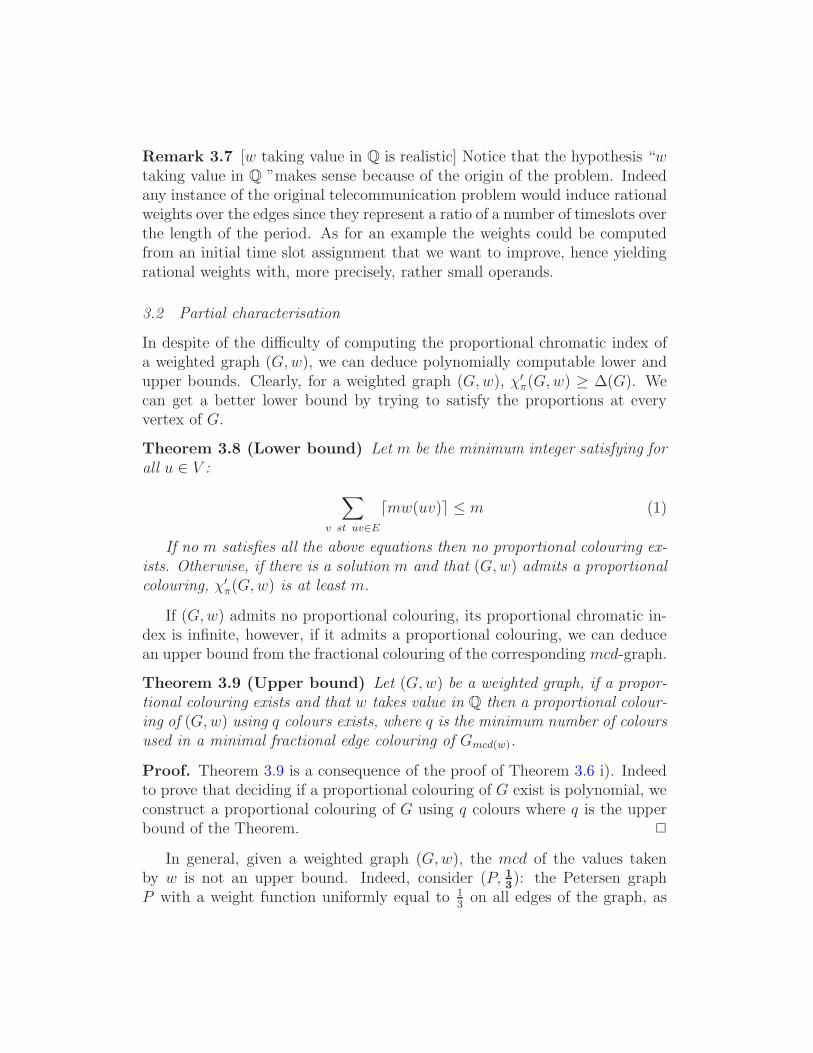
Remark 3.7 [w taking value in Q is realistic] Notice that the hypothesis “wtaking value in Q ”makes sense because of the origin of the problem. Indeedany instance of the original telecommunication problem would induce rationalweights over the edges since they represent a ratio of a number of timeslots overthe length of the period. As for an example the weights could be computedfrom an initial time slot assignment that we want to improve, hence yieldingrational weights with, more precisely, rather small operands.
3.2 Partial characterisation
In despite of the difficulty of computing the proportional chromatic index ofa weighted graph (G, w), we can deduce polynomially computable lower andupper bounds. Clearly, for a weighted graph (G, w), χ′
π(G, w) ≥ ∆(G). Wecan get a better lower bound by trying to satisfy the proportions at everyvertex of G.
Theorem 3.8 (Lower bound) Let m be the minimum integer satisfying forall u ∈ V :
∑
v st uv∈E
⌈mw(uv)⌉ ≤ m (1)
If no m satisfies all the above equations then no proportional colouring ex-ists. Otherwise, if there is a solution m and that (G, w) admits a proportionalcolouring, χ′
π(G, w) is at least m.
If (G, w) admits no proportional colouring, its proportional chromatic in-dex is infinite, however, if it admits a proportional colouring, we can deducean upper bound from the fractional colouring of the corresponding mcd-graph.
Theorem 3.9 (Upper bound) Let (G, w) be a weighted graph, if a propor-tional colouring exists and that w takes value in Q then a proportional colour-ing of (G, w) using q colours exists, where q is the minimum number of coloursused in a minimal fractional edge colouring of Gmcd(w).
Proof. Theorem 3.9 is a consequence of the proof of Theorem 3.6 i). Indeedto prove that deciding if a proportional colouring of G exist is polynomial, weconstruct a proportional colouring of G using q colours where q is the upperbound of the Theorem. 2
In general, given a weighted graph (G, w), the mcd of the values takenby w is not an upper bound. Indeed, consider (P, 1
3): the Petersen graph
P with a weight function uniformly equal to 13
on all edges of the graph, as
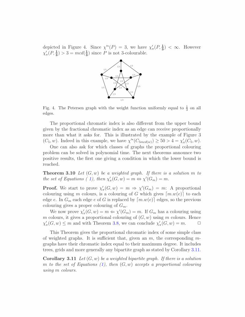
depicted in Figure 4. Since χ′∗(P ) = 3, we have χ′π(P, 1
3) < ∞. However
χ′π(P, 1
3) > 3 = mcd(1
3) since P is not 3-colourable.
1/3
1/3
1/3
1/3
1/3
1/3
1/3 1/3
1/3
1/31/3
1/3
1/3
1/31/3
Fig. 4. The Petersen graph with the weight function uniformly equal to 13 on all
edges.
The proportional chromatic index is also different from the upper boundgiven by the fractional chromatic index as an edge can receive proportionallymore than what it asks for. This is illustrated by the example of Figure 3(C5, w). Indeed in this example, we have χ′∗(C5mcd(w)) ≥ 50 > 4 = χ′
π(C5, w).
One can also ask for which classes of graphs the proportional colouringproblem can be solved in polynomial time. The next theorems announce twopositive results, the first one giving a condition in which the lower bound isreached.
Theorem 3.10 Let (G, w) be a weighted graph. If there is a solution m tothe set of Equations ( 1), then χ′
π(G, w) = m ⇔ χ′(Gm) = m.
Proof. We start to prove χ′π(G, w) = m ⇒ χ′(Gm) = m: A proportional
colouring using m colours, is a colouring of G which gives ⌈m.w(e)⌉ to eachedge e. In Gm each edge e of G is replaced by ⌈m.w(e)⌉ edges, so the previouscolouring gives a proper colouring of Gm.
We now prove χ′π(G, w) = m ⇐ χ′(Gm) = m. If Gm has a colouring using
m colours, it gives a proportional colouring of (G, w) using m colours. Henceχ′
π(G, w) ≤ m and with Theorem 3.8, we can conclude χ′π(G, w) = m. 2
This Theorem gives the proportional chromatic index of some simple classof weighted graphs. It is sufficient that, given an m, the corresponding m-graphs have their chromatic index equal to their maximum degree. It includestrees, grids and more generally any bipartite graph as stated by Corollary 3.11.
Corollary 3.11 Let (G, w) be a weighted bipartite graph. If there is a solutionm to the set of Equations (1), then (G, w) accepts a proportional colouringusing m colours.

Proof. Given a weighted bipartite graph (G, w) with a solution m to theEquations (1), the maximun degree of Gm is m. Observe that Gm is alsobipartite and hence is edge chromatic number is m: χ′(Gm) = m and so theprevious theorem gives the result. 2
If G is an outerplanar (a planar graph which has a planar representationsuch that all edges are incident to the unbounded face) which is not an oddcycle, Theorem 3.10 also includes the weighted graphs (G, w) if w is a weightfunction uniform on all edges. Indeed, we know that a simple outerplanar isof class 1 iff it is not an odd cycle. Hence an outerplanar which is not anodd cycle and such that all edges have the same multiplicity has its chromaticindex equals to its maximum degree. Given a weighted outerplanar graph(G, w) with w constant, for any m, Gm is an outerplanar graph with all edgeshaving the same multiplicity, its maximum degree is m and hence χ′(Gm) = m.For m solution to the set of Equations (1), Theorem 3.10 applies.
Recall that the condition w uniform over all edges is not sufficient sincewe proved Theorem 3.6 using a weighted graph which has a constant weightfunction. Furthermore, if G is an outerplanar but w is not uniform on alledges then we can not conclude using Theorem 3.10. To see this, consider asimple outerplanar graph G with a triangle, a weigth function w and m thesolution to the Equations (1). If w is such that the m-graph Gm has too manymultiple edges on a triangle it may not have edge chromatic index m. Figure 5presents an outerplanar G and an outerplanar with multiple edges which maybe an m-graph of G. In this example we have a triangle with edge multiplicity4 which forces the chromatic index to be at least 12 while the maximun degreeof the multiple graph is 10.
Fig. 5. Example of an outerplanar G with multiple edges and χ′(G) 6= ∆(G).
We can also give more information on the proportional chromatic index ofa weighted graph if its weight function verifies some properties. Next Theoremgoes in this direction:
Theorem 3.12 Let (G, w) be a weighted graph with w taking values in Q.Let e be an edge with an end vertex v such that
∑uv∈E w(uv) = 1. Then,
the denominator of w(e) divides the number of colours used in a proportionalcolouring of (G, w), in particular it divides χ′
π(G, w).
Proof. Consider a proportional colouring of (G, w) using m colours. Lete be an edge with an end vertex v such that
∑uv∈E w(uv) = 1. We have∑
uv∈E⌈m.w(uv)⌉ ≤ m =∑
uv∈E m.w(uv). Hence ⌈m.w(e)⌉ = m.w(e). It isin particular true for m = χ′
π(G, w). 2
Remark 3.13 [why w should takes value in Q] As Remark 3.7 says, the originof the problem justifies the hypothesis that w takes value in Q. In the contextof this Theorem, there is a second reason. Indeed, if at a vertex v where theweights sum at 1,
∑uv∈E w(uv) = 1, we have an irrational weight then the
set of Equations (1) do not have a solution, which means that no proportionalcolouring exist.
From Theorem 3.12, we can deduce the following corollary:
Corollary 3.14 Let (G, w) be a weighted graph. If the proportional chro-matic number of (G, w) is finite and every edge e has an end vertex v with∑
uv∈E w(uv) = 1, then χ′π(G, w) = mcd(w).
Notice that we do not need the hypothesis “w taking values in Q ”fromthe above remark.
Proof. The previous Theorem implies that mcd(w) is a lower bound. Since,by Theorem 3.9 it is also an upper bound, the result follows. 2
In a weighted graph (G, w), a vertex v with∑
uv∈E w(uv) = 1, representsa saturated node, i.e. a node through which no extra request can be routed.A weighted graph (G, w) with w taking values in Q such that every edge isincident to a saturated vertex represents a saturated network, i.e. a network inwhich no extra request can be routed. The previous corollary gives the valueof the proportional chromatic index of such a network.
The presence of a saturated node also allows to have an inapproximabilityresult:
Corollary 3.15 Given a weighted graph (G, w) with w taking values in Q anda vertex v such that
∑uv∈E w(uv) = 1. Let q be the mcd of w(uv), uv ∈ E.
χ′π(G, w) is not approximable within the constant q − 1.
Proof. Theorem 3.12 implies that q divides the number of colours used in aproportional colouring, hence no proportional colouring exist with χ′
π(G, w)+icolours for 0 < i < q. 2

4 Conclusion
Motivated by the applications modelled by the proportional colouring problemand its hardness, we let the following general open questions: find approxima-tion algorithms for classes of graphs which usually occur in telecommunication,as circular-arc graphs and triangular lattices and determine other classes ofgraphs (and weighted classes of graphs) for which the proportional chromaticindex can be calculated in polynomial time.
References
[1] I. Akyildiz, X. Wang, and W. Wang, “Wireless mesh networks: a survey,”Computer Networks, vol. 47, no. 4, pp. 445–487, 2005.
[2] H. Liu and B. Zhao, “Optimal scheduling for link assignment in traffic-sensitivestdma wireless ad-hoc networks,” in ICCNMC, ser. LNCS, vol. 3619, 2005, pp.218–228.
[3] R. Klasing, N. Morales, and S. Perennes, “On the complexity of bandwidthallocation in radio networks with steady traffic demands,” Theoretical ComputerScience, 2008, to appear.
[4] J. Bibb Cain, T. Billhartz, L. Foore A link scheduling and ad hoc networkingapproach using directional antennas, Military comm. conf., 1 Oct 2003, 643–648.
[5] Carlson, R.C. and Nemhauser, G.L., Scheduling to minimize interaction cost,Oper. Res. 14 (1966), 52–58.
[6] Holyer, I. The NP-completeness of edge colourings, SIAM J. Computing 10(1981), 718–720.
[7] Koreas, D.P., The NP-completeness of chromatic index in triangle free graphswith maximum vertex of degree 3, App. Math. and Comp. 83 (1) (1997), 13–17.
[8] McDiarmid, C., Discrete mathematics and radio channel assignment, In: Recentadvances in algorithms and combinatorics, eds. B. Reed and C. Linhares-Sales,Springer, New York, 2003, 27–63.
[9] Padberg, M. and Rao, M., Odd minimum cutsets and b-matchings, Math. Oper.Res. 7 (1982), 67–80.
[10] Vizing, V.G., On an estimate of a chromatic class of a p-graph (In Russian),Diskret. Analiz. 3 (1964), 25–30.

228 Annexes

Annexe C
Réseaux d’accès et de cœur
C.1 WDM and Directed Star Arboricity
Article soumis à Combinatorics, Probability and Computing.
C.2 Muticast Routing and Wavelength Assignment in Pas-sive Optical Access Networks
Coming soon.
229

WDM and directed star arboricity
Omid Amini∗ Frederic Havet∗ Florian Huc∗ Stephan Thomasse†
Abstract
A digraph is m-labelled if every arc is labelled by an integer in 1, . . . , m. Motivated by wavelengthassignment for multicasts in optical networks, we study n-fiber colourings of labelled digraphs. Theseare colourings of the arcs of D such that at each vertex v, and for each colour λ, in(v, λ)+out(v, λ) ≤ n
with in(v, λ) the number of arcs coloured λ entering v and out(v, λ) the number of labels l suchthat there is at least one arc of label l leaving v and coloured with λ. The problem is to find theminimum number of colours λn(D) such that the m-labelled digraph D has an n-fiber colouring. Inthe particular case, when D is 1-labelled, λn(D) is called the directed star arboricity of D, and isdenoted by dst(D). We first show that dst(D) ≤ 2∆−(D)+1 and conjecture that if ∆−(D) ≥ 2 thendst(D) ≤ 2∆−(D). We also prove that if D is subcubic then dst(D) ≤ 3 and that if ∆+(D), ∆−(D) ≤2 then dst(D) ≤ 4. Finally, we study λn(m,k) = maxλn(D) | D is m-labelled and ∆−(D) ≤ k.
We show that if m ≥ n then
‰
m
n
‰
k
n
ı
+k
n
ı
≤ λn(m, k) ≤
‰
m
n
‰
k
n
ı
+k
n
ı
+ Cm2 log k
nfor some
constant C. We conjecture that the lower bound should be the right value of λn(m, k).
1 Introduction
The origin of this paper is the study of wavelength assignment for multicasts in star network. Partialresults are already obtained by Brandt and Gonzalez [4]. We are given a star network in which a centralnode is connected by optical fibers to a set of nodes V . The nodes of V communicates together usingWDM (wavelength-division multiplexing), hence different signals may be sent at the same time throughthe same fiber but on different wavelengths. The central node is an all-optical transmitter which canredirect a signal arriving from a node on a particular wavelength to some (one or more) of the othersnodes on the same wavelength. It means that the central node is able to duplicate a message incoming ona wavelength to different fibers without changing its wavelength. Therefore if a node v send a multicastto a set of nodes S(v), v should send the message to the central node on a set of wavelengths so that thecentral node redirect it to each node of S(v) using one of these wavelengths. The aim is to minimize thetotal number of used wavelengths.
We first study the very fundamental case when the fiber is unique and each vertex v sends a uniquemulticast M(v) to a set S(v) of nodes. Let D be the digraph with vertex set V such that the outneigh-bourhood of a vertex v is S(v). Note that this is a digraph and not a multidigraph (there is no multiplearcs) as S(v) is a set. Then the problem is to find the smallest k such that there exists a mappingφ : V (D) → 1, . . . , k satisfying the two conditions:
(i) φ(uv) 6= φ(vw);
(ii) φ(uv) 6= φ(u′v).
∗Projet Mascotte, CNRS/INRIA/UNSA, INRIA Sophia-Antipolis, 2004 route des Lucioles BP 93, 06902 Sophia-AntipolisCedex, France. oamini,fhavet,[email protected]. These authors are partially supported by the European projectAEOLUS
†LIRMM, 161 rue ADA, Montpellier, [email protected]
1

Such a mapping is called directed star k-colouring. The directed star arboricity of a digraph D, denotedby dst(D), is the minimum integer k such that there exists a directed star k-colouring. This notion hasbeen introduced in [6] and is an analog of the star arboricity defined in [1]. An arborescence is a connecteddigraph in which every vertex has indegree 1 except one, called root, which has indegree 0. A forest isthe disjoint union of arborescences. A star is an arborescence in which the root dominates all the othervertices. A galaxy is a forest of stars. Clearly, every colour class of a directed star colouring is a galaxy.Hence, the directed star arboricity of a digraph D is the minimum number of galaxies into which A(D)may be partitioned.
For a vertex v, its indegree d−(v) corresponds to the number of multicasts it receives. A sensibleassumption is that a node receives a bounded number of multicasts. Hence, Brandt and Gonzalez [4]studied the directed star arboricity of a digraph D with regards to its maximum indegree. The maximumindegree of a digraph D, denoted ∆−(D) or simply ∆−, is maxd−(v) | v ∈ V (D). Brandt and Gonzalezshowed that dst(D) ≤ ⌈5∆−/2⌉. This upper bound is tight if ∆− = 1 because odd circuits have directedstar arboricity 3. However it can be improved for larger value of ∆−. We conjecture that if ∆− ≥ 2, thendst(D) ≤ 2∆−.
Conjecture 1 Every digraph D with maximum indegree ∆− ≥ 2 satisfies dst(D) ≤ 2∆−.
This conjecture would be tight as Brandt [3] showed that for every ∆−, there is an acyclic digraphD∆− with maximum indegree ∆− and dst(D∆−) = 2∆−. Note that to prove this conjecture, it issufficient to prove it for ∆− = 2 and ∆− = 3. Indeed a digraph with maximum indegree ∆− ≥ 2 has anarc-partition into ∆−/2 digraphs with maximum indegree 2 if ∆− is even, and into (∆− − 1)/2 digraphswith maximum indegree 2 and one with maximum indegree 3 if ∆− is odd. In section 2, we show thatdst(D) ≤ 2∆− + 1 and settle Conjecture 1 for acyclic digraphs.
Remark 2 Note that we restrict ourselves to simple digraphs, i.e. circuits of length two are permitted,but not multiple arcs. When multiple arcs are allowed, all the bounds above do not hold. Indeed, givenan integer ∆−, the multidigraph T∆− with three vertices u, v and w and ∆− parallel arcs uv, vw andwu satisfies dst(T∆−) = 3∆−. Moreover, this example is extremal since every multidigraph satisfiesdst(D) ≤ 3∆−. Indeed let us show it by induction: pick a vertex v with outdegree at most ∆− in aterminal strong component. A strong component C of a digraph is terminal if there is no arc leavingC, i.e. with tail in C and head outside of C. If v has no inneighbour, it is isolated and we removeit. Otherwise, we consider any arc uv. Its colour must be different from the colours of the d−(u) arcsentering u, the d+(v) arcs leaving v and the d−(v) − 1 other arcs entering v, so at most 3∆− − 1 arcsin total. Hence, remove the arc uv, apply induction, and extend the colouring to uv. Therefore, formultidigraphs, the bound dst(D) ≤ 3∆− is sharp.
We then study the directed star arboricity of a digraph with bounded maximum degree. The degreeof a vertex v is d(v) = d−(v) + d+(v). It corresponds to the degree of the vertex in the underlyingmultigraph. (We have edges with multiplicity 2 in the underlying multigraph each time there is a circuitof length two in the digraph.) The maximum degree of a digraph D, denoted ∆(D), or simply ∆ when Dis clearly understood from the context, is maxd(v), v ∈ V (D). Let us denote by µ(G), the maximummultiplicity of an edge in a multigraph. By Vizing’s theorem, one can colour the edges of a multigraphwith ∆(G)+µ(G) colours so that two edges have different colours if they are incident. Since the multigraphunderlying a digraph has maximum multiplicity at most two, for any digraph D, dst(D) ≤ ∆ + 2. Weconjecture the following:
Conjecture 3 Let D be a digraph with maximum degree ∆ ≥ 3. Then dst(D) ≤ ∆.
This conjecture would be tight since every digraph with ∆ = ∆− has directed star arboricity at least ∆.In section 3, we prove that Conjecture 3 holds when ∆ = 3.
2

Pinlou and Sopena [9] studied a stronger form of directed star arboricity, called acircuitic directedstar arboricity. They add the extra condition that any circuit has to have at least three distinct colours.Note that such a notion applies only to oriented graphs that are digraphs without circuit of length 2.Indeed such a circuit may not receive 3 colours. They showed that the acircuitic directed star arboricityof a subcubic (i.e. each vertex has degree at most 3) oriented graph is at most four. We give a new andvery short proof of this result.
A first step towards Conjectures 1 and 3 would be to prove the following statement which is weakerthan these two conjectures.
Conjecture 4 Let k ≥ 2 and D be a digraph. If max(∆−, ∆+) ≤ k then dst(D) ≤ 2k.
This conjecture holds and is far from being tight for large values of k. Indeed Guiduli [6] showed thatif max(∆−, ∆+) ≤ k then dst(D) ≤ k + 20 log k + 84. Guiduli’s proof is based on the fact that, whenboth out and indegree are bounded, the colour of an arc depends on the colour of few other arcs. Thisbounded dependency allows the use of the Lovasz Local Lemma. This idea was first used by Algor andAlon [1], for the star arboricity of undirected graphs. Note also that Guiduli’s result is (almost) tightsince there are digraphs D with max(∆−, ∆+) ≤ k and dst(D) ≥ k + Ω(log k) (see [6]). Furthermore, asfor Conjecture 1, it is sufficient to prove Conjecture 4 for k = 2 and k=3. In Section 4, we prove thatConjecture 4 holds for k = 2. By the above remark, it implies that Conjecture 4 holds for all even k.
In Section 5, we investigate the complexity of finding the directed star arboricity of a digraph. Un-surprisingly, this is an NP-hard problem. More precisely, we show that determining the directed stararboricity of a digraph with out- and indegree at most 2 is NP-complete.
Next, we study the more general (and more realistic) problem in which the center is connectedto the nodes of V with n optical fibers. Moreover each node may send several multicasts. We noteM1(v), . . . , Ms(v)(v) the s(v) multicasts that node v send. For 1 ≤ i ≤ s(v), the set of nodes to whichthe multicast Mi(v) is sent is denoted by Si(v). The problem is still to find the minimun number ofwavelength used considering that all fibers are identical.
We model it as a labelled digraph problem: We consider a digraph D on vertex set V . For eachmulticast Mi(v) = (v, Si(v)), v ∈ V , 1 ≤ i ≤ s(v), we add the set of arcs Ai(v) = vw, w ∈ Si(v) withlabel i. The label of an arc a is denoted by l(a). Thus for every couple (u, v) of vertices and label i thereis at most one arc uv labelled by i. If each vertex sends at most m multicasts, there are at most m labelson the arcs. Such a digraph is said to be m-labelled. One wants to find an n-fiber wavelength assignmentof D, that is a mapping Φ : A(D) → Λ×1, . . . , n×1, . . . n in which every arc uv is associated a triple(λ(uv), f+(uv), f−(uv)) such that :
(i) (λ(uv), f−(uv)) 6= (λ(vw), f+(vw));
(ii) (λ(uv), f−(uv)) 6= (λ(u′v), f−(u′w));
(iii) if l(vw) 6= l(vw′) then (λ(vw), f+(vw)) 6= (λ(vw′), f+(vw′)).
λ(uv) corresponds to the wavelength of uv, and f+(uv) and f−(uv) the fiber used in u and v respec-tively. Hence we can describe the equations as follow:
(i) corresponds to the fact that an arc entering v and an arc leaving v have either different wavelengthor different fibers;
(ii) corresponds to the fact that two arcs entering v have either different wavelength or different fibers;
(iii) corresponds to the fact that two arcs leaving v with different labels have either different wavelengthsor different fibers.
3
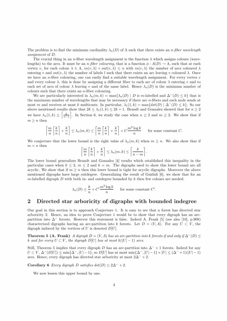
The problem is to find the minimum cardinality λn(D) of Λ such that there exists an n-fiber wavelengthassignment of D.
The crucial thing in an n-fiber wavelength assignment is the function λ which assigns colours (wave-lengths) to the arcs. It must be an n-fiber colouring, that is a function φ : A(D) → Λ, such that at eachvertex v, for each colour λ ∈ Λ, in(v, λ) + out(v, λ) ≤ n with in(v, λ) the number of arcs coloured λentering v and out(v, λ) the number of labels l such that there exists an arc leaving v coloured λ. Oncewe have an n-fiber colouring, one can easily find a suitable wavelength assignment. For every vertex vand every colour λ, this is done by assigning a different fiber to each arc of colour λ entering v and toeach set of arcs of colour λ leaving v and of the same label. Hence λn(D) is the minimum number ofcolours such that there exists an n-fiber colouring.
We are particularly interested in λn(m, k) = maxλn(D) | D is m-labelled and ∆−(D) ≤ k that isthe maximum number of wavelengths that may be necessary if there are n-fibers and each node sends atmost m and receives at most k multicasts. In particular, λ1(1, k) = maxdst(D) | ∆−(D) ≤ k. So ourabove mentioned results show that 2k ≤ λ1(1, k) ≤ 2k + 1. Brandt and Gonzalez showed that for n ≥ 2
we have λn(1, k) ≤⌈
kn−1
⌉
. In Section 6, we study the case when n ≥ 2 and m ≥ 2. We show that if
m ≥ n then
⌈
m
n
⌈
k
n
⌉
+k
n
⌉
≤ λn(m, k) ≤
⌈
m
n
⌈
k
n
⌉
+k
n
⌉
+ Cm2 log k
nfor some constant C.
We conjecture that the lower bound is the right value of λn(m, k) when m ≥ n. We also show that ifm < n then
⌈
m
n
⌈
k
n
⌉
+k
n
⌉
≤ λn(m, k) ≤
⌈
k
n − m
⌉
.
The lower bound generalizes Brandt and Gonzalez [4] results which established this inequality in theparticular cases when k ≤ 2, m ≤ 2 and k = m. The digraphs used to show this lower bound are allacyclic. We show that if m ≥ n then this lower bound is tight for acyclic digraphs. Moreover the abovementioned digraphs have large outdegree. Generalizing the result of Guiduli [6], we show that for anm-labelled digraph D with both in- and outdegree bounded by k then few colours are needed:
λn(D) ≤k
n+ C′m
2 log k
nfor some constant C′.
2 Directed star arboricity of digraphs with bounded indegree
Our goal in this section is to approach Conjecture 1. It is easy to see that a forest has directed stararboricity 2. Hence, an idea to prove Conjecture 1 would be to show that every digraph has an arc-partition into ∆− forests. However this statement is false. Indeed A. Frank [5] (see also [10], p.908)characterized digraphs having an arc-partition into k forests. Let D = (V, A). For any U ⊂ V , thedigraph induced by the vertices of U is denoted D[U ].
Theorem 5 (A. Frank) A digraph D = (V, A) has an arc-partition into k forests if and only if ∆−(D) ≤k and for every U ⊂ V , the digraph D[U ] has at most k(|U | − 1) arcs.
Still, Theorem 5 implies that every digraph D has an arc-partition into ∆− + 1 forests. Indeed for anyU ⊂ V , ∆−(D[U ]) ≤ min∆−, |U |− 1, so D[U ] has at most min∆−, |U |− 1× |U | ≤ (∆− +1)(|U |− 1)arcs. Hence, every digraph has directed star arboricity at most 2∆− + 2.
Corollary 6 Every digraph D satisfies dst(D) ≤ 2∆− + 2.
We now lessen this upper bound by one.
4

Theorem 7 Every digraph D satisfies dst(D) ≤ 2∆− + 1.
The idea to prove Theorem 7 is to show that every digraph has an arc-partition into ∆− forests and agalaxy G. To do so, we prove a stronger result (Lemma 8) by induction.
A sink is a vertex with outdegree 0. A source is a vertex with indegree 0. Let D be a multidigraph.It is k-nice if ∆− ≤ k and if the tails of parallel arcs, if any, are sources. A k-decomposition of D is anarc-partition into k forests and a galaxy G such that every source of D is isolated in G. Let u be a vertexof D. A k-decomposition of D is u-suitable if no arc of G has head u.
Lemma 8 Let u be a vertex of a k-nice multidigraph D. Then D has a u-suitable k-decomposition.
Proof. We proceed by induction on n + k. We now discuss the connectivity of D:
• If D is not connected, we apply induction on every component.
• If D is strongly connected, every vertex has indegree at least one. Remember also that there is noparallel arcs. Let v be an outneighbour of u. There exists a spanning arborescence T with root vwhich contains all the arcs with tail v. Let D′ be the digraph obtained from D by removing the arcsof T and v. Observe that D′ is (k−1)-nice. By induction, it has a u-suitable (k−1)-decomposition(F1, . . . , Fk−1, G). Note that the Fi, 1 ≤ i ≤ k − 1, T and G contain all the arcs of D except thosewith head v. By construction, G′ = G∪uv is a galaxy since no arc of G has head u. Let u1, . . . , ul−1
be the inneighbours of v distinct from u, where l ≤ k. Let F ′i = Fi ∪uiv, for all 1 ≤ i ≤ l− 1. Then
each F ′i is a forest, so (F1, . . . , Fk−1, T, G′) is a u-suitable k-decomposition of D.
• If D is connected but not strongly connected, we consider a strongly connected terminal componentD1. Set D2 = D \D1. Let u1 and u2 be two vertices of D1 and D2, respectively, such that u is oneof them.
If D2 has a unique vertex v (thus u2 = v), since D is connected and D1 is strong, there exists aspanning arborescence T of D with root v. Now D′ = D \ A(T ) is a (k − 1)-nice multidigraph, soby induction it has a u-suitable (k − 1)-decomposition. Adding T to this decomposition, we obtaina u-suitable k-decomposition.
If D2 has more than one vertex, by induction, it admits a u2-suitable k-decomposition (F 21 , . . . , F 2
k , G2).Moreover the digraph D′
1 obtained by contracting D2 to a single vertex v is k-nice and so has au1-suitable k-decomposition (F 1
1 , . . . , F 1k , G1). Moreover, since v is a source, it is isolated in G1.
Hence G = G1 ∪ G2 is a galaxy. We now let Fi be the union of F 1i and F 2
i by replacing the arcsof F 1
i with tail v by the corresponding arcs in D. Then (F1, . . . , Fk, G) is a k-decomposition of Dwhich is suitable for both u1 and u2.
2.1 Acyclic digraphs
It is not hard to show that dst(D) ≤ 2∆− when D is acyclic, but we will prove this result in a moreconstrained way. A cyclic n-interval of 1, 2, . . . , p is a set of n consecutive numbers modulo p. Nowfor the directed star colouring, we will insist that for every vertex v, the (distinct) colours used to colourthe arcs with head v are chosen in a cyclic k-interval of 1, 2, . . . , 2k. Thus, the number of possiblesets of colours used to colour the entering arcs of a vertex drastically falls from
(
2kk
)
when every set is apriori possible, to 2k. Note that having consecutive colours on the arcs entering a vertex corresponds tohaving consecutive wavelengths on the link between the corresponding node and the central one. This isvery important for grooming issues. For more details about grooming, we refer to the two comprehensivesurveys [7, 8].
5

Theorem 9 Let D be an acyclic digraph with maximum indegree k. D admits a directed star 2k-colouringsuch that for every vertex, the colours assigned to its entering arcs are included in a cyclic k-interval of1, 2, . . . , 2k.
To prove this result, we need the following result on set of distinct representatives.
Lemma 10 Let I1, . . . , Ik be k non necessary distinct cyclic k-intervals of 1, 2, . . . , 2k. Then I1, . . . , Ik
admit a set of distinct representatives forming a cyclic k-interval.
Proof. We consider I1, . . . , Ik as a set of p distinct cyclic k-intervals I1, . . . , Ip with respective multiplicitym1, . . . , mp such that
∑pi=1 mi = k. Such a system will be denoted by ((I1, m1), . . . , (Ip, mp)). We shall
prove the existence of a cyclic k-interval J , such that J can be partitioned into p subsets Ji, 1 ≤ i ≤ p,such that |Ji| = mi and Ji ⊂ Ii. This proves the lemma (by associating distinct elements of Ji to eachcopy of Ii).
We proceed by induction on p. The result holds trivially for p = 1. We have two cases:
• There exists i and j such that |Ij \ Ii| = |Ii \ Ij | ≤ max(mi, mj).
Suppose without loss of generality that i < j and mi ≥ mj . We apply the induction hypothesis to((I1, m1), · · · , (Ii, mi + mj), · · · , (Ij−1, mj−1), (Ij+1, mj+1), · · · , (Ip, mp)), in order to find a cyclicinterval J ′, such that J ′ admits a partition into subsets J ′
r, such that for any r 6= i, j, J ′r ⊂ Ir is
a subset of size mr, and J ′i ⊂ Ii is of size mi + mj . We now partition J ′
i into two sets Ji and Jj
with respective size mi and mj , in such a way that (Ii \ Ij)∩ J ′i ⊆ Ji. Remark that this is possible
exactly because of our assumption |Ij \ Ii| = |Ii \ Ij | ≤ mi. Since Ji ⊂ Ii and Jj ⊂ Ij , this refinedpartition of J ′ is the desired one.
• For any i, j we have |Ij \ Ii| = |Ii \ Ij | ≥ max(mi, mj) + 1.
Each Ii intersects exactly 2mi − 1 other cyclic k-intervals on less than mi elements. Since thereare 2k cyclic k-intervals in total and
∑pi=1(2mi − 1) = 2k − p < 2k, we conclude the existence of a
cyclic k-interval J which intersects each Ii in an interval of size at least mi.
Let us prove that one can partition J in the desired way. By Hall’s matching theorem, it sufficesto prove that for every subset I of 1, . . . , p, |
⋃
i∈I Ii ∩ J | ≥∑
i∈I mi.
Suppose for a contradiction that a subset I of 1, . . . , p violates this inequality. Such a subsetwill be called contracting. Without loss of generality, we assume that I is a contracting set withminimum cardinality and that I = 1, . . . , q. Remark that by the choice of J , we have q ≥ 2.The set K :=
⋃
i∈I Ii ∩ J consists of one or two intervals of J , each containing one extremity ofJ . By the minimality of I, K must be a single interval (if not, one would take I1 (resp. I2),all the elements of I which contains the first (resp. the second) extremity of J . Then one ofI1 or I2 would be contracting). Thus, one of the two extremities of J is in every Ii, i ∈ I.Without loss of generality, we may assume that (I1 ∩ J) ⊂ (I2 ∩ J) ⊂ · · · ⊂ (Iq ∩ J). Now,for every 2 ≤ i ≤ q, |Ii \ Ii−1| = |(Ii ∩ J) \ (Ii−1 ∩ J)| ≥ max(mi, mi−1) + 1 ≥ mi + 1. But|⋃
i∈I Ii ∩ J | = |(I1 ∩ J)| +∑q
i=2 |(Ii ∩ J) \ (Ii−1 ∩ J)|. So |⋃
i∈I Ii ∩ J | ≥∑q
i=1 mi + q − 1, whichis a contradiction.
Proof of Theorem 9. By induction on the number of vertices, the result being trivial if D has onevertex. Suppose now that D has at least two vertices. Then D has a sink x. By the induction hypothesis,D \ x has a directed star 2k-colouring c such that for every vertex, the colours assigned to its enteringarcs are included in a cyclic k-interval. Let v1, v2, . . . , vl be the inneighbours of x in D, where l ≤ kbecause ∆−(D) ≤ k. For each 1 ≤ i ≤ l, let I ′i be a cyclic k-interval which contains all the colours of the
6

arcs with head vi. We set Ii = 1, . . . , 2k \ I ′i. Clearly, Ii is a cyclic k-interval and the arc vix can becoloured by any element of Ii. By Lemma 10, I1, . . . , Il have a set of distinct representatives included ina cyclic n-interval J . Hence assigning J to x, and colouring the arc vix by the representative of Ii givesa directed star 2k-colouring of D.
Theorem 9 is tight : Brandt [3] showed that for every k, there is an acyclic digraph such that∆−(Dk) = k and dst(Dk) = 2k. His construction is the special case for n = m = 1 of the constructiongiven in Proposition 21.
3 Subcubic digraphs
Recall that a subcubic digraph is a graph with degree at most three. In this section, we first show thatthe directed star arboricity of a subcubic digraph is at most 3, so proving Conjecture 3 when ∆ = 3. Wethen give a very short proof of a result of Pinlou and Sopena asserting that the acircuitic directed stararboricity of a subcubic digraph is at most 4.
3.1 Directed star arboricity of subcubic digraphs
The aim of this subsection is to prove the following theorem:
Theorem 11 Every subcubic digraph has directed star arboricity at most 3.
To do so, we need to establish some lemmas to enable us to extend some partial directed star colouringinto directed star colouring of the whole digraph. These lemmas need the following definition. LetD = (V, A) be a digraph and S a subset of V ∪ A. Suppose that each element x of S is assigned a listL(x). A colouring c of S is an L-colouring if c(x) ∈ L(x) for every x ∈ S.
Lemma 12 Let C be a circuit in which every vertex v receives a list L(v) of two colours among 1, 2, 3and each arc a receives the list L(a) = 1, 2, 3. Then there is no L-colouring c of the arcs and verticessuch that c(x) 6= c(xy), c(y) 6= c(xy), and c(xy) 6= c(yz), for all arcs xy and yz if and only if C is oddand all the vertices have the same list.
Proof. Assume first that every vertex is assigned the same list, say 1, 2. If C is odd, it is simplematter to see that we can not find the desired colouring. Indeed, among two consecutive arcs, one has tobe coloured 3. If C is even, we colour the vertices by 1 and the arcs alternately by 2 and 3.
Now assume that C = x1x2 . . . xkx1 and x1 and x2 are assigned different lists. Say L(x1) = 1, 2and L(x2) = 2, 3. We colour the arc x1x2 by 3, the vertex x2 by 2 and the arc x2x3 by 1. Then wecolour x3, x3x4, . . . , xk. It remains to colour xkx1 and x1. Two cases may happen: If we can colourxkx1 by 1 or 2, we do it and colour x1 by 2 or 1 respectively. Otherwise the set of colours assigned to xk
and xk−1xk is 1, 2. Hence, we colour xkx1 with 3, x1 by 1, and recolour x1x2 by 2 and x2 by 3.
Lemma 13 Let D be a subcubic digraph with no vertex of outdegree two and indegree one. Assume thatevery arc a has a list of colours L(a) ⊂ 1, 2, 3 such that:
• If the head of a is a sink s (a is called a final arc), |L(a)| ≥ d−(s).
• If a is not a final arc and the tail of a is a source (a is called an initial arc), |L(a)| ≥ 2.
• In other cases |L(a)| = 3.
• If a vertex is the head of at least two initial arcs the union of their lists of colours contains at leastthree colours.
7

• If all the vertices of an odd circuit are the tails of initial arcs, the union of the lists of colours ofthese initial arcs contains at least three colours.
Then D has a directed star L-colouring.
Proof. We colour the graph inductively. Consider a terminal strong component C of D. Since D hasno vertex with indegree one and outdegree two, C induces either a singleton or a circuit.
1) Assume that C is a singleton v which is the head of a unique arc a = uv. If u has indegree 0, coloura with a colour of its list. If u has indegree 1, and thus total degree 2, colour a by the colour ofits list and remove this colour from the list of the arc with head u. If u is the head of e and f ,observe that L(e) and L(f) have at least two colours and their union have at least three colours. Toconclude, colour a with a colour in its list, remove this colour from L(e) and L(f), remove a, splitu into two vertices, one with head e, and the other with head f . Now, choose in their respectivelists different colours for the arcs e and f to form the new list L(e) and L(f).
2) Assume that C is a singleton v which is the head of several arcs, including a = uv. In this case, wereduce L(a) to a single colour, remove this colour from the other arcs with head v and split v intov1 which becomes the head of a, and v2 which becomes the head of the other arcs.
3) Assume that C is a circuit. Every arc entering C has a list of at least two colours. We can applyLemma 12 to conclude.
Proof of Theorem 11. Assume for contradiction that the digraph D has directed star arboricity morethan three and is minimum with respect to the number of arcs for this property. Observe that D hasno source, otherwise we simply delete it with its incident arcs, apply induction and extend the colouringsince arcs leaving from a source can be coloured arbitrarily. Let D1 be the subdigraph of D induced bythe vertices of indegree at most 1. We denote by D2 the digraph induced by the other vertices, and by[Di, Dj ] the set of arcs with tail in Di and head in Dj. We claim that D1 contains no even circuit. Ifnot, we simply remove the arcs of this even circuit, apply induction and extend the colouring to the arcsof the even circuit since every arc of the circuit has two colours available.
A critical set of vertices of D2 is either a vertex of D2 with indegree at least two in D1, or an oddcircuit of D2 having all its inneighbours in D1. Observe that critical sets are disjoint. For every criticalset S, we select two arcs entering S from D1, called selected arcs of S.
Let D′ be digraph induced by the arc set A′ = A(D1) ∪ [D2, D1]. Now we define a conflict graph onthe arcs of D′ in the following way:
• Two arcs xy, yv of D′ are in conflict, called normal conflict at y.
• Two arcs xy, uv of D′ are also in conflict if there exists two selected arcs of the same set S withtails y and v. These conflicts are called selected conflicts at y and v.
Let us analyse the structure of the conflict graph. Observe first that an arc is in conflict with threearcs : one normal conflict at its tail and at most two (normal or selected) at its head.
We claim that there is no K4 in the conflict graph. Suppose there is one, then there are four arcspairwise in conflict. Since each arc has degree 3, it has a normal conflict at its tail, the digraphs inducedby these four arcs contains a circuit. It cannot be a circuit of even length (2 or 4) so it has length 3. Itfollows that the four arcs a, b, c, d are as in Figure 1 below. Let D∗ be the digraph obtained from D byremoving the arcs a, b, c, d and their four incident vertices. By minimality of D, D∗ admits a directed star3-colouring which can be extended to D as depicted below depending if the two leaving arcs are colouredthe same or differently. This proves the claim.
8
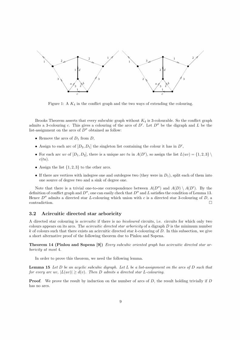
21
3
3
112
2
3
1
21
3
3
121
2
3
2
a b
c
d
a b
c
d
Figure 1: A K4 in the conflict graph and the two ways of extending the colouring.
Brooks Theorem asserts that every subcubic graph without K4 is 3-colourable. So the conflict graphadmits a 3-colouring c. This gives a colouring of the arcs of D′. Let D′′ be the digraph and L be thelist-assignment on the arcs of D′′ obtained as follow:
• Remove the arcs of D1 from D,
• Assign to each arc of [D2, D1] the singleton list containing the colour it has in D′,
• For each arc uv of [D1, D2], there is a unique arc tu in A(D′), so assign the list L(uv) = 1, 2, 3 \c(tu).
• Assign the list 1, 2, 3 to the other arcs.
• If there are vertices with indegree one and outdegree two (they were in D1), split each of them intoone source of degree two and a sink of degree one.
Note that there is a trivial one-to-one correspondence between A(D′′) and A(D) \ A(D′). By thedefinition of conflict graph and D′′, one can easily check that D′′ and L satisfies the condition of Lemma 13.Hence D′′ admits a directed star L-colouring which union with c is a directed star 3-colouring of D, acontradiction.
3.2 Acircuitic directed star arboricity
A directed star colouring is acircuitic if there is no bicoloured circuits, i.e. circuits for which only twocolours appears on its arcs. The acircuitic directed star arboricity of a digraph D is the minimum numberk of colours such that there exists an acircuitic directed star k-colouring of D. In this subsection, we givea short alternative proof of the following theorem due to Pinlou and Sopena.
Theorem 14 (Pinlou and Sopena [9]) Every subcubic oriented graph has acircuitic directed star ar-boricity at most 4.
In order to prove this theorem, we need the following lemma.
Lemma 15 Let D be an acyclic subcubic digraph. Let L be a list-assignment on the arcs of D such thatfor every arc uv, |L(uv)| ≥ d(v). Then D admits a directed star L-colouring.
Proof. We prove the result by induction on the number of arcs of D, the result holding trivially if Dhas no arcs.
9
Since D is acyclic, it has an arc xy with y a sink. Let a be a colour in L(xy). For any arc e distinctfrom xy, set L′(e) = L(e) \ a if e incident to xy (and thus has head in x, y since y is a sink), andL′(e) = L(e) otherwise. Then in D′ = D − xy, we have |L′(uv)| ≥ d(v). Hence, by induction hypothesis,D′ admits a directed star L′-colouring that can be extended in a directed star L-colouring of D bycolouring xy with a.
Proof of Theorem 14.Let V1 be the set of vertices of outdegree at most 1 and V2 = V \ V1. Then every vertex of V2 has
outdegree at least 2 and so indegree at most 1.Let M be the set of arcs with tail in V1 and head in V2. Colour all the arcs of M with 4. Moreover
for every circuit C in D[V1] and D[V2] choose an arc e(C) and colour it by 4. Note that, by definition ofV1 and V2, the arc e(C) is not incident to any arc of M and C is the unique circuit containing e(C). Letus denote M4 the set of arcs coloured 4. Then M4 is a matching and D − M4 is acyclic.
We shall now find a directed star colouring of D−M4 with 1, 2, 3 that creates any bicoloured circuit.If such a circuit exists, 4 would be one of its colour because D − M4 is acyclic and all its arcs coloured4 would be in M because the arcs of M4 \ M is in a unique circuit which has a unique arc coloured 4.Hence we just have to be careful when colouring arcs in the digraph induced by the endvertices of thearcs of M .
Let us denote the arcs of M by xiyi, 1 ≤ i ≤ p and set X = xi, 1 ≤ i ≤ p and Y = yi, 1 ≤ i ≤ p.Then xi ∈ V1 and yi ∈ V2. Let E′ be the set of arcs with tail in Y and head in X . Let H be the graphwith vertex set E′ such that an arc yixj is adjacent to an arc ykxl if
(a) either k = l,
(b) or j = k and i > j and l > j.
Since a vertex of X has indegree at most 2 and a vertex of Y has outdegree at most 2, H has maximumdegree 3. Moreover H contains no K4 because two arcs of E′ with same tail yk are not adjacent in H .Hence, by Brooks Theorem, H has a vertex-colouring in 1, 2, 3 which is corresponds to a colouring cof the arcs of E′. Since (a) is satisfied c is a directed star colouring. Moreover this colouring creates nobicoloured circuits: indeed a circuit contains a subpath yixjyjxl with i > j and k > j, whose three arcsare coloured differently by (b).
Let D′ = D − (M4 ∪ E′). For any arc uv in D′, let L(uv) = 1, 2, 3 \ c(wv) | wv ∈ E′. Theset L(uv) is the set of colours in 1, 2, 3 that may be assigned to uv without creating any conflict withthe already coloured arcs. D′ is acyclic and |L(uv)| ≥ d(v), so by Lemma 15, it admits a directed starL-colouring and thus D has an acircuitic directed star colouring in 1, 2, 3, 4.
Remark 16 Note that in the acircuitic directed star 4-colouring provided in the proof of Theorem 14the arcs coloured 4 form a matching.
4 Directed star arboricity of digraphs with maximum in and
outdegree two
The goal of this section is to prove that every digraph with outdegree and indegree at most two hasdirected star arboricity at most four.
Theorem 17 Let D be a digraph. If ∆− ≤ 2 and ∆+ ≤ 2, then dst(D) ≤ 4.
Thus, Conjecture 4 holds for k = 2 and hence for all even k. However, the class of digraphs with in andoutdegree at most two is certainly not an easy class with respect to directed star arboricity, as we willshow in Section 5.
10

In order to prove Theorem 17, it suffices to show that D contains a galaxy G which spans all thevertices of degree four. Then D′ = D − A(G) has maximum degree at most 3. So, by Theorem 11,dst(D′) ≤ 3, so dst(D) ≤ 4. Hence Theorem 17 is directly implied by the following lemma:
Lemma 18 Let D be a digraph with maximum indegree and outdegree two. Then D contains a galaxywhich spans the set of vertices with degree four.
In order to prove this lemma, we need some preliminaries:Let V be a set. An ordered digraph on V is a pair (≤, D) where:
• ≤ is a partial order on V .
• D is a digraph with vertex set V .
• D contains the Hasse diagram of ≤ (i.e. when x ≤ y ≤ z implies x = y or y = z, then xz is an arcof D).
• If xy is an arc of D, the vertices x, y are ≤-comparable.
The arcs xy of D thus belong to two different types: the forward arcs when x ≤ y, and the backwardarcs when y ≤ x.
Lemma 19 Let (≤, D) be an ordered digraph on V . Assume that every vertex is the tail of at most onebackward arc and at most two forward arcs and that the indegree of every vertex of D is at least 2, exceptpossibly one vertex x with indegree 1. Then D contains two arcs ca and bd such that a ≤ b ≤ c, b ≤ dand c 6≤ d, all four vertices being distinct except possibly a = b.
Proof. Let us consider a counterexample with minimum |V |.An interval is a subset I of V which has a minimum m and a maximum M such that I = z :
m ≤ z ≤ M. An interval I is good if every arc with tail in I and head outside I has tail M and everybackward arc in I has tail M .
Let I be an interval of D. The digraph D/I obtained from D by contracting I is the digraph withvertex set (V \ I) ∪ vI such that xy is an arc if and only either vI /∈ x, y and xy ∈ A(D), or x = vI
and there exists xI ∈ I such that xIy ∈ A(D), or y = vI and there exists yI ∈ I such that xyI ∈ A(D).Similarly, the binary relation ≤/I obtained from ≤ by contracting I is the binary relation on (V \ I)∪
vI such that x ≤/I y if and only if either vI /∈ x, y and x ≤ y, or x = vI and there exists xI ∈ I suchthat xI ≤ y, or y = vI and there exists yI ∈ I such that x ≤ yI . We claim that if I is good then ≤/I isa partial order. Indeed suppose it is not, there are two elements u and t such that u ≤/I vI , vI ≤ t andu 6≤/I t. Then M 6≤ t. Let a ∈ I be the a maximal element of I such that a ≤ t, d be a successor of ain I and c a successor of a not in I (it exists as t /∈ I and a ≤ t and maximal in I with this property).Then d and c are incomparable and ac and ad are in the Hasse diagram of ≤ then because I is good itfollows that ca and ad are arcs of D, which is impossible as D is a counterexample.
Hence if I is a good interval, (≤/I , D/I) is an ordered digraph. Note that if x ≤/I vI then x ≤ Mwith M the maximum of I. The crucial point is that if I a good interval of D for which the conclusionof Lemma 19 holds for (≤/I , D/I), then it holds for (≤, D). Indeed, suppose there exists two arcs ca andbd of D/I such that a ≤/I b ≤/I c, b ≤/I d and c 6≤/I d. Note that since I is good vI 6= c. Let M be themaximum of I.If vI /∈ a, b, c, d, then ca and bd gives the conclusion for D.If vI = a then cM is an arc. Let us show that M ≤ b. Indeed let x be a maximal vertex in I such thatx ≤ b and y a minimal vertex such that x ≤ y ≤ b. Since the Hasse diagram of ≤ is included in D thenxy is an arc so x = M since I is good. Thus cM and bd are the desired arcs.
11
If vI = b then Md is an arc and a ≤ M , so ca and Md are the desired arcs.If vI = d then there exists dI ∈ I such that bdI , so ca and bdI are the desired arcs.
Hence to get a contradiction, it is sufficient to find a good interval I such that (≤/I , D/I) satisfiesthe hypotheses of Lemma 19.
Observe that there are at least two backward arcs. Indeed, if there are two minimal elements for ≤,there are at least three backward arcs entering these vertices (since one of them can be x). And if thereis a unique minimum m, by letting m′ minimal in V \ m, at least two arcs are entering m, m′.
Let M be a vertex which is the tail of a backward arc and which is minimal for ≤ for this property.Since two arcs cannot have the same tail, M is not the maximum of ≤ (if any). Let Mm be the backwardarc with tail M .
We claim that the interval J with minimum m and maximum M is good. Indeed, by the definitionof M , no backward arc has its tail in J \ M. Moreover, any forward arc bd with its tail in J \ M andits head outside J would give our conclusion (with a = m and c = M), a contradiction.
Now consider a good interval I with maximum M which is maximal with respect to inclusion. Weclaim that if x ∈ I, then there is at least one arc entering I, and if x /∈ I, there are at least two arcsentering I with different tails.
Call m1 the minimum of I and m2 any minimal element of I \m1. First assume that x is in I. Thereare at least three arcs with heads m1 or m2. One of them is m1m2, one of them can be with tail M , butthere is still one left with tail not in I. Now assume that x is not in I. There are at least two arcs withheads m1 or m2 and tails not in I. If the tails are different, we are done. If the tails are the same, say v,observe that vm1 and vm2 are both backward of both forward (otherwise v would be in I). Since bothcan not be backward vm1 and vm2 are forward. Hence the interval with minimum v and maximum Mis a good interval, contradicting the maximality of I. This proves the claim.
This claim implies that (≤/I , D/I) satisfies the hypotheses of Lemma 19, yielding a contradiction.
Proof of Theorem 18. Let G be a galaxy of D which spans a maximum number of vertices of degreefour. Suppose for contradiction that some vertex x with degree four is not spanned.
An alternating path is an oriented path ending at x, starting by an arc of G, and alternating with arcsof G and arcs of A(D) \A(G). We denote by A the set of arcs of G which belong to an alternating path.
Claim 1 Every arc of A is a component of G.
Proof. Indeed, if uv belongs to A, it starts some alternating path P . Thus, if u has outdegree morethan one in G, the digraph with set of arcs A(G)A(P ) is a galaxy and spans V (G) ∪ x.
Claim 2 There is no circuits alternating arcs of A and arcs of A(D) \ A.
Proof. Assume that there is such a circuit C. Consider a shortest alternating path P starting withsome arc of A in C. Now the digraph with arcs A(G)(A(P )∪A(C)) is a galaxy which spans V (G)∪ x,contradicting the maximality of G.
We now endow A∪x with a partial order structure by letting a ≤ b if there exists an alternating pathstarting at a and ending at b. The fact that this relation is a partial order relies on Claim 2. Observethat x is the maximum of this order.
We also construct a digraph D on vertex set A ∪ x and all arcs uv → st such that us or vs is an arcof D (and uv → x such that ux or vx is an arc of D).
Claim 3 The pair (D,≤) is an ordered digraph. Moreover an arc of A is the tail of at most one backwardarc and two forward arcs and x is the tail of at most two backward arcs.
12

Proof. The fact that the Hasse diagram of ≤ is contained in D follows from the fact that if uv ≤ stbelongs to the Hasse diagram of ≤, there is an alternating path starting by uvst, in particular, the arcvs belongs to D, and thus uv → st in D.
Suppose that uv → st and then vs or us is an arc of D. If vs is an arc, then because there is noalternating circuit, st follows uv on some alternating path so uv ≤ st. In this case, uv → st is forward.If us is an arc of D, we claim that st ≤ uv. Indeed, if an alternating path P starting at st does notcontain uv, the galaxy with arcs (A(G)A(P )) ∪ us spans V (G) ∪ x contradicting the maximality ofG. In this case, uv → st is backward.
It follows that an arc uv of A is the tail of at most one backward arc since this arc and uv are the twoarcs leaving u in D and the tail of at most two forward arcs since v has outdegree at most 2. Furthermore,since x has outdegree at most two, it follows that x is the tail of at most two backward arcs.
Claim 4 The indegree of every vertex of D is two.
Proof. Let uv be a vertex of D which starts an alternating path P . If u has indegree less than two,and thus does not belong to the set of vertices of degree four, the galaxy with arcs A(G)A(P ) spansmore vertices of degree four than G, a contradiction. Let s and t be the two inneighbours of u in D. Anelement of A ∪ x contains s otherwise the galaxy with arcs (A(G)A(P )) ∪ su spans V (G) ∪ x andcontradicts the maximality of G. Similarly an element of A∪ x contains t.
Observe that the same element of A∪ x cannot contain both s and t (either the arc st or the arc ts),otherwise the arcs su and tu would be both backward or forward, which is impossible.
At this stage, in order to apply Lemma 19, we just need to insure that the backward outdegree ofevery vertex is at most one. Since the only element of D which is the tail of two backward arcs is x, wesimply delete any of these two backward arcs. The indegree of a vertex of D decreases by one but we arestill fulfilling the hypothesis of Lemma 19.
Hence according to this lemma, D contains two arcs ca and bd such that a ≤ b ≤ c, b ≤ d and c 6≤ d.Keep in mind that a, b, c, d are elements of A∪x. In particular, there is an alternating path P containinga, b, d (in this order) which does not contain c. Setting a = a1a2 and c = c1c2, note that the backwardarc ca corresponds to the arc c1a1 in D. We reach a contradiction by considering the galaxy with arcs(A(G)A(P )) ∪ c1a1 which spans V (D′) ∪ x.
5 Complexity
The digraphs with directed star arboricity 1 are the galaxies, so one can polynomially decide if dst(D) = 1.Deciding whether dst(D) = 2 or not is also easy since we just have to check that the conflict graph (withvertex set the arcs of D, two distinct arcs xy, uv being in conflict when y = u or y = v) is bipartite.However for larger value, as expected, it is NP-complete to decide if a digraph has directed star arboricityat most k. This is illustrated by the next result:
Theorem 20 The following problem is NP-complete:INSTANCE: A digraph D with ∆+(D) ≤ 2 and ∆−(D) ≤ 2.QUESTION: Is dst(D) at most 3?
Proof. The proof is a reduction to 3-edge-colouring of 3-regular graphs. To see this, consider a 3-regular graph G. It admits an orientation D such that every vertex has in and outdegree at least 1. LetD′ be the digraph obtained from D by replacing every vertex with indegree 1 and outdegree 2 by thesubgraph H depicted in Figure 2 which has also one entering arc (namely a) and two leaving arcs (b and
13

a1
b
c2
1
3
3
22
3
1
2
3
1
Figure 2: The graph H and one of its directed star 3-colouring
c). It is easy to check that in any directed star 3-colouring of H , the three arcs a, b and c get differentcolours. Moreover if these three arcs are precoloured with three different colours, we can extend this to adirected star 3-colouring of H . Such a colouring with a coloured 1, b coloured 2 and c coloured 3 is givenin Figure 2. Furthermore, a vertex with indegree 2 and outdegree 1 must have its three incident arcscoloured differently in a directed star 3-colouring. So dst(D′) = 3 if and only if G is 3-edge colourable.
6 Multiple fibers
In this section we consider the problem with n ≥ 2 fibers. More precisely, we give some bounds onλn(m, k). We first give a lower bound on λn(m, k).
Proposition 21 λn(m, k) ≥
⌈
m
n
⌈
k
n
⌉
+k
n
⌉
Proof. Consider the following m-labelled digraph Gn,m,k with vertex set X ∪ Y ∪ Z such that :
• |X | = k, |Y | = 2(m+1)k2
and |Z| = m(
|Y |k
)
.
• For any x ∈ X and y ∈ Y there is an arc xy (of whatever label).
• For every set S of k vertices of Y and integer 1 ≤ i ≤ m, there is a vertex ziS in Z which is dominated
by all the vertices of S via arcs labelled i.
Suppose there exists an n-fiber colouring of Gn,m,k with c <⌈
mn
⌈
kn
⌉
+ kn
⌉
colours. For y ∈ Y and1 ≤ i ≤ m, let Ci(y) be the set of colours assigned to the arcs labelled i leaving y. For 0 ≤ j ≤ n, let Pj theset of colours used on j arcs entering y (and necessarily with two different fibers). Then
∑nj=0 j|Pj | = k
as k arcs enter y. Moreover (P0, P1, . . . , Pn) is a partition of the set of colours so∑n
j=0 |Pj | = c. Noweach colour of Pj may appear in at most n − j of the Ci(y), so
m∑
i=1
|Ci(y)| ≤n
∑
j=0
(n − j)|Pj | = n
n∑
j=0
|Pj | −n
∑
j=0
j|Pj | = cn − k.
Because |Y | = 2(m+1)k2
, there is a set S of k vertices y of Y having the same m-uple (C1(y), . . . , Cm(y)) =(C1, . . . , Cm). Without loss of generality, we may assume |C1| = min|Ci| | 1 ≤ i ≤ m. Hence|C1| ≤ cn−k
m . But the vertex z1S has indegree k so |C1| ≥ k/n. Since |C1| is an integer, we have
14

⌊
cn−km
⌋
≥ |C1| ≥ ⌈k/n⌉. So c ≥ mn
⌈
kn
⌉
+ kn . Since c is an integer, we get c ≥
⌈
mn
⌈
kn
⌉
+ kn
⌉
, acontradiction.
Note that the graph Gn,m,k is acyclic. The following lemma shows that, if m ≥ n, one cannot expectbetter lower bounds by considering acyclic digraphs. Indeed Gn,m,k is the m-labelled acyclic digraphwith indegree at most k for which an n-fiber colouring requires the more colours.
Lemma 22 Let D be an acyclic m-labelled digraph with ∆− ≤ k. If m ≥ n then λn(D) ≤⌈
mn
⌈
kn
⌉
+ kn
⌉
.
Proof. Since D is acyclic, its vertex set admits an ordering (v1, v2, . . . , vp) such that if vjvj′ is an arcthen j < j′.
By induction on q, we shall find an n-fiber colouring of D[v1, . . . , vq] together with sets Ci(vr),1 ≤ i ≤ m and 1 ≤ r ≤ q, of ⌈k/n⌉ colours such that, in the future, assigning a colour in Ci(vr) to an arclabelled i leaving vr will fulfill the condition of n-fiber colouring at vr.
Starting the process is easy. We may take as Ci(v1) any ⌈k/n⌉-sets such that a colour appears in atmost n of them.
Suppose now that we have an n-fiber colouring of D[v1, . . . , vq−1] and that, for 1 ≤ i ≤ m and1 ≤ r ≤ q − 1, the set Ci(vr) is determined. Let us colour the arcs entering vq. Each of these arcs vrvq
may be assigned one of the ⌈k/n⌉ colours of Cl(vrvq)(vr). Since a colour may be assigned to n arcs (usingdifferent fibers) entering vq, one can assign a colour and fiber to each such arc. It remains to determinethe Ci(vq), 1 ≤ i ≤ m.
For 0 ≤ j ≤ n, let Pj be the set of colours assigned to j arcs entering vq. Let N =∑n
i=0(n − j)|Pj |and (c1, c2, . . . , cN ) be a sequence of colours such that each colour of Pj appears exactly n− j times andconsecutively. For 1 ≤ i ≤ m, set Ci(vq) = ca | a ≡ i mod m. As n ≤ m, a colour appears at mostonce in each Ci(vq). Moreover, N = n
⌈
mn
⌈
kn
⌉
+ kn
⌉
− k ≥ m⌈
kn
⌉
. So for 1 ≤ i ≤ m, |Ci(vq)| ≥⌈
kn
⌉
.
Lemma 22 shows that the lower bound of Proposition 21 is tight for acyclic digraphs. In fact, weconjecture that is it tight also for digraphs in general:
Conjecture 23 λn(m, k) =
⌈
m
n
⌈
k
n
⌉
+k
n
⌉
We now establish an upper bound on λn(m, k) for general digraphs. To do so, we first give an upperbound on λn(D) for m-labelled digraphs with bounded in- and outdegree In this case, one can derive fromthe following theorem of Guiduli that “few” colours are needed. Note that the graphs Gn,m,k requireslots of colours but have very large outdegree.
Theorem 24 (Guiduli [6]) If ∆−, ∆+ ≤ k then dst(D) ≤ k + 20 log k + 84. Moreover D admitsa directed star colouring with k + 20 log k + 84 colours such that for each vertex v there are at most10 log k + 42 colours assigned to its leaving arcs.
The proof of Guiduli’s Theorem can be modified to obtain the following statement for m-labelleddigraphs.
Theorem 25 Let f(n, m, k) =
⌈
k + (10m2 + 5) log k + 80m2 + m + 21
n
⌉
and D be an m-labelled digraph
with ∆−, ∆+ ≤ k. Then λn(D) ≤ f(n, m, k). Moreover D admits an n-fiber colouring with f(n, m, k)such that for each vertex v and each label l, there are at most g(m, k) = ⌈(10m + 5) log k + 40m + 21⌉colours assigned to the arcs labelled l leaving v.
Note that Theorem 25 in the case n = m = 1 is a bit better than Theorem 24. Indeed it shows that if∆−, ∆+ ≤ k then dst(D) ≤ k + 15 log k + 102. It is due to Lemma 7 which is a bit better than Guiduli’sone because it uses Theorem 7 (dst ≤ 2∆− + 1) whereas Guiduli uses dst ≤ 3∆−. However the methodis identical.
15

Definition 26 Given a family of sets F = (Ai, i ∈ I) A transversal of F is a family of distinct elements(ti, i ∈ I) with ∀i, ti ∈ Ai.
Lemma 27 Let D be a m-labelled digraph with ∆− ≤ k. Suppose that for each vertex v, there arem disjoint lists L1
v, ..., Lmv of c colours each being a subset of 1, ..., k + c. If for each vertex v, the
family Liy | yx ∈ E(D) and yx is labelled i has a transversal, then there is a 1-fiber colouring of D with
k + (2m2 + 1)c + m colours such that for each vertex v and label l, at most (2m + 1)c + 1 colours areassigned to arcs labelled l leaving v.
Proof. Using the transversal to colour the entering arcs at each vertex, we obtain a colouring with fewconflicts. Indeed there is no conflict between arcs entering a same vertex. So the only possible conflictare between an arc entering a vertex v and an arc leaving v. Since arcs leaving v use at most m.c colours(those of L1
v ∪ ... ∪ Lmv ), there are at most m.c arcs entering v having the same colour as an arc leaving
c. Removing such entering arcs for every vertex v, we obtain a digraph D′ for which the colouring withthe k + c colours is a 1-fiber colouring. We now want to colour the arcs of D−D′ with few extra colours.Consider a label 1 ≤ l ≤ m, let D′
l be the digraph induced by the arcs of D −D′ labelled l. Then D′l has
indegree at most m.c. By Theorem 7, we can partition D′l in 2m.c+1 star forests. Thus D can be 1-fiber
coloured with k + c + m(2m.c + 1) colours. Moreover, in the above described colouring, arcs labelled lleaving a vertex v have a colour in Ll
v or corresponding to one of the 2m.c + 1 star forests of D′l. So at
most (2m + 1)c + 1 colours are assigned to arcs labelled l leaving v.
Theorem 28 (N. Alon, C. McDiarmid, B. Reed, 1992 [2]) Let k and c be positive integers withk ≥ c ≥ 5 log k + 20. Choose independent random subsets S1, . . . , Sk of X = 1, . . . , k + c as follows.For each i choose Si by performing c independent uniform samplings from X. Then the probability thatS1, . . . , Sk do not have a transversal is at most k3− c
2
Proof of Theorem 25. It suffices to prove the result for n = 1. Indeed we can extend a 1-fiber colouringsatisfying the conditions of the theorem to a n-fiber colouring satisfying the conditions by replacing thecolour qn + r with 1 ≤ r ≤ n by the colour q + 1 on fiber r.
Let c = ⌈5 log k + 20⌉ We can assume k ≥ m.c. For all vertices x, select m.c different ordered elementse1, e2, · · · , em.c independently and uniformly. For all 1 ≤ i ≤ m, let Li
x = eci+1, · · · , ec(i+1). Each sethas the same distribution as the c elements where chosen uniformly and independently.
Let Ax be the event that the family Liy | yx ∈ E(D) and yx is labelled i fails to have a transversal.
By Theorem 28, P (Ax) ≤ k3−c/2. Furthermore, the event Ax is independent of all Ay for which there isno vertex z such that both zx and zy are in E(D). The dependency graph for the events has degree atmost k2 so we can apply Lovasz Local Lemma. We obtain that there exists a family of lists satisfyingconditions of Lemma 27. This lemma gives the desired colouring.
Any digraph D may be decomposed into an acyclic digraph Da and an eulerian digraph De, that issuch that for every vertex v, d−De
(V ) = d+De
(v). Indeed consider an eulerian subdigraph De of D which hasa maximum number of arcs. Then the digraph Da = D−De is necessarily acyclic. Hence by Theorems 25and 22, if m ≥ n then λn(D) ≤
⌈
mn
⌈
kn
⌉
+ kn
⌉
+ f(n, m, k). But we will now lessen this bound by roughlykn .
Theorem 29 If n ≤ m, then
λn(m, k) ≤
⌈
m
n
⌈
k
n
⌉
+k
n
⌉
+ 2m⌈(10m + 5) log k + 40m + 21⌉
n.
16

Proof. Let D be an m-labelled digraph with ∆−(D) ≤ k. Consider a decomposition of D into aneulerian digraph De and an acyclic digraph Da. We first apply Theorem 25 and n-fiber colour the arcs ofDe with f(n, m, k) colours such that at most g(m, k) colours are assigned to the arcs leaving each vertex.
We shall extend the n-fiber colouring of De to the arcs of Da in a way similar to the proof of Lemma 22,i.e. we will assign to each vertex v sets Ci(v), 1 ≤ i ≤ m of ⌈k/n + m.g(m, k)⌉ colours such that an arclabelled i leaving v will be labelled using a colour in Ci(v).
Let (v1, . . . , vn) be an ordering of the vertices of A such that if vjvj′ is an arc then j < j′.We start to build the Ci(v1) with the colours assigned to the leaving arcs of v1 labelled i. The vertex
v1 has at most k entering arcs. Each of them forbid one type (colour, fiber). In the colouring of De
induced by Theorem 25, there are at most m.g(m, k) types assigned to the arcs leaving v1. So there are
at least⌈
mkn2
⌉
+⌈
kn
⌉
+ 2m g(m,k)n − k − m.g(m, k) ≥ m
⌈
kn
⌉
+ m.g(m, k) types unused at vertex v1. Since
n ≤ m, we can partition these types into m sets of size at least kn such that no two types having the same
colour are in the same set. These sets are the Ci(v1).Suppose that the sets have been defined for v1 up to vq−1 and that all the arcs vivj for i < q and
j < q have a colour. We now give a colour to the arcs of type vivq for i < q.There are ke arcs entering vq in De which are already coloured. So it remains to give a colour to
ka ≤ k− ke arcs. Each uncoloured arc may be assigned a colour in a list of size at least⌈
kn + m.g(m, k)
⌉
.
This gives a choice between n.⌈
kn + m.g(m, k)
⌉
different types. ke types are forbidden by the enteringarcs in De while at most m.g(m, k) types are forbidden by the leaving arcs in De. Then it remains atleast n.
⌈
kn + m.g(m, k)
⌉
− ke − m.g(m, k) ≥ ka types for each entering arcs of Da. So one can assigndistinct available colours to each of the ka arcs entering vq.
We then build the Ci(vq) as we did for v1.
This process finished, we obtain an n-fiber colouring of D using⌈
mkn2
⌉
+⌈
kn
⌉
+ 2m g(m,k)n colours.
Theorem 29 gives an upper bound on λn(m, k) when m ≥ n. We now give one when m < n.
Proposition 30 If m < n then λn(m, k) ≤⌈
kn−m
⌉
.
Proof. Let D be an m-labelled digraph with ∆− ≤ k. For each vertex v, we give to its entering arcsa colour such that none of them is used more than n − m times. This is possible as there are at most
k ≤ (n − m)⌈
kn−m
⌉
arcs entering v. Then we have in(v, λ) ≤ n − m. Moreover each arc vw is given a
colour by w. Since D is m-labelled, a colour λ can be used to colour an arc of at most m different labels,i.e. out(v, λ) ≤ m. Consequently in(v, λ) + out(v, λ) ≤ n. This gives a proper n-fiber colouring.
References
[1] I. Algor and N. Alon, The star arboricity of graphs, Discrete Mathematics 75 (1989), 11–22.
[2] N. Alon, C. McDiarmid, B. Reed, Star arboricity, Combinatorica 12 (1992), 375–380.
[3] R. Brandt, Multicasting using WDM in Multifiber Optical Star Networks, Thesis, UCSB, Sep 2003.
[4] R. Brandt and T. F. Gonzalez, Wavelength assignment in multifiber optical star networks underthe multicasting communication mode, Journal of Interconnection Networks 6 (2005), 383–405.
[5] A. Frank, Covering branchings, Acta Sci. Math. (Szeged) 41 (1979), 77–81.
[6] B. Guiduli, On incidence coloring and star arboricity of graphs, Discrete Mathematics 163 (1997),275–278.
17

[7] A. Lardies, R. Gupta and R. Patterson. Traffic grooming in a multi-layer network. Opt. Netw.Mag., 2 (2001), 91–99.
[8] E. Modiano and P.J. Lin. Traffic grooming in WDM networks. IEEE Communications Magazine,39(7), (2001), 124–129.
[9] A. Pinlou and E. Sopena, The acircuitic directed star arboricity of subcubic graph is at most four,Discrete Mathematics, to appear.
[10] A. Schrijver, Combinatorial optimization. Polyhedra and efficiency. Algorithms and Combinatorics24, Springer-Verlag, Berlin, 2003.
7 Appendix
7.1 Alternative proof of Theorem 14
In this subsection, we give an alternative proof of Theorem 14 using Theorem 11.Proof. As every subcubic digraph is the subgraph of a cubic digraph, its suffices to prove the result forcubic digraph. So let D be a cubic digraph by Theorem 11, it admits a directed star 3-colouring c.
We will now select one arc eC per bicoloured circuit C and recolour it with 4. If C is dominating(no arcs enters C) or is dominated (no arcs leaves C) let eC be any arc of C, otherwise let eC be an arcwhose tail has indegree 2 and head outdegree 2.
It is easy to see that the set of arcs now coloured 4 is a matching. Note moreover that the arcs incidentto an arc uv coloured 4 have their colours in the set of two colours 1, 2, 3 \ c where c is the colourinitially assigned to uv.
The way we have selected the recoloured arcs assures us that we have a 4-directed star colouring.Moreover, there is no circuits bicoloured with two colours in 1, 2, 3. However, we may have bicolouredcircuits with arcs coloured 4, so we need to do an extra recolouring. Note that the arcs coloured 4 ofsuch circuits were not selected for dominating or dominated circuits.
An arc uv coloured 4 may be in at most 2 bicoloured circuit and if it is in two such circuits, let sayC1 bicoloured 4 and c1 and C2 bicoloured 4 and c2 with c1 6= c2, the two circuits enter u and leave v withdifferent arcs. Now for each bicoloured circuit C, we choose an arc fC coloured 4 in order to maximizethe number of arcs chosen by two circuits.
Recolour each arc uv that has been chosen by two circuits, let say C1 bicoloured 4 and c1 and C2
bicoloured 4 and c2, with the colour c3 ∈ 1, 2, 3\c1, c2. Doing so we still have a directed star colouringand the circuit C1 and C2 are no more bicoloured. Moreover, we do not create any new bicoloured circuit:indeed, a circuit C containing the arc uv must go through one of the two arcs vw1 of C1 and vw2 ofC2, which are coloured c1 and c2 respectively. Wlog it uses uw1. But w1 has outdegree one and the arcleaving w1 is in both C and C1 and so is coloured 4. Hence the three colours c3, ci and 4 appears on C.
We will now recolour an arc of each remaining bicoloured circuit C one after another. Such a re-colouring will make C no more bicoloured and create no new bicoloured circuits. Hence at the end, wewill have a 4-acircuitic directed star colouring of D.
Let us consider such a circuit C. Its chosen arc uv has been chosen only once. Note that uv does notbelong to any other such circuit since the number of arc chosen twice is maximized. In particular, allthe arcs incident to uv have not been recoloured. Let tu be the arc preceding uv in C. Recolour tu withthe colour c3 in 1, 2, 3 \ c1, c2. This is valid since u is the head of an arc coloured 4 and thus hasoutdegree 2. Moreover, it does not create any bicoloured circuit since all the circuits containing tu mustcontain one of the arcs leaving v which are coloured using a colour of c1, c2.
18
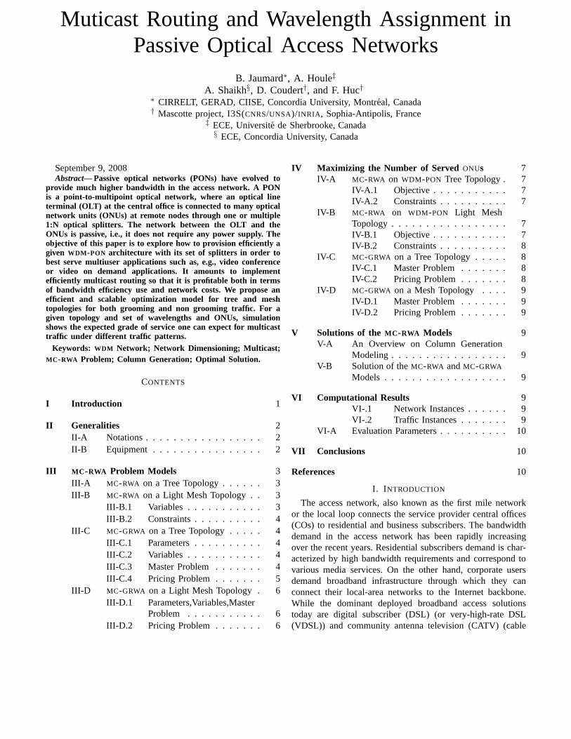
Muticast Routing and Wavelength Assignment inPassive Optical Access Networks
B. Jaumard∗, A. Houle‡
A. Shaikh§, D. Coudert†, and F. Huc†∗ CIRRELT, GERAD, CIISE, Concordia University, Montreal, Canada† Mascotte project, I3S(CNRS/UNSA)/INRIA , Sophia-Antipolis, France
‡ ECE, Universite de Sherbrooke, Canada§ ECE, Concordia University, Canada
September 9, 2008Abstract— Passive optical networks (PONs) have evolved to
provide much higher bandwidth in the access network. A PONis a point-to-multipoint optical network, where an optical lineterminal (OLT) at the central office is connected to many opticalnetwork units (ONUs) at remote nodes through one or multiple1:N optical splitters. The network between the OLT and theONUs is passive, i.e., it does not require any power supply. Theobjective of this paper is to explore how to provision efficiently agiven WDM -PON architecture with its set of splitters in order tobest serve multiuser applications such as, e.g., video conferenceor video on demand applications. It amounts to implementefficiently multicast routing so that it is profitable both in termsof bandwidth efficiency use and network costs. We propose anefficient and scalable optimization model for tree and meshtopologies for both grooming and non grooming traffic. For agiven topology and set of wavelengths and ONUs, simulationshows the expected grade of service one can expect for multicasttraffic under different traffic patterns.
Keywords: WDM Network; Network Dimensioning; Multicast;MC -RWA Problem; Column Generation; Optimal Solution.
CONTENTS
I Introduction 1
II Generalities 2II-A Notations . . . . . . . . . . . . . . . . . 2II-B Equipment . . . . . . . . . . . . . . . . 2
III MC -RWA Problem Models 3III-A MC-RWA on a Tree Topology . . . . . . 3III-B MC-RWA on a Light Mesh Topology . . 3
III-B.1 Variables . . . . . . . . . . . 3III-B.2 Constraints . . . . . . . . . . 4
III-C MC-GRWA on a Tree Topology . . . . . 4III-C.1 Parameters . . . . . . . . . . 4III-C.2 Variables . . . . . . . . . . . 4III-C.3 Master Problem . . . . . . . 4III-C.4 Pricing Problem . . . . . . . 5
III-D MC-GRWA on a Light Mesh Topology . 6III-D.1 Parameters,Variables,Master
Problem . . . . . . . . . . . 6III-D.2 Pricing Problem . . . . . . . 6
IV Maximizing the Number of Served ONUs 7IV-A MC-RWA on WDM-PON Tree Topology . 7
IV-A.1 Objective . . . . . . . . . . . 7IV-A.2 Constraints . . . . . . . . . . 7
IV-B MC-RWA on WDM-PON Light MeshTopology . . . . . . . . . . . . . . . . . 7IV-B.1 Objective . . . . . . . . . . . 7IV-B.2 Constraints . . . . . . . . . . 8
IV-C MC-GRWA on a Tree Topology . . . . . 8IV-C.1 Master Problem . . . . . . . 8IV-C.2 Pricing Problem . . . . . . . 8
IV-D MC-GRWA on a Mesh Topology . . . . 9IV-D.1 Master Problem . . . . . . . 9IV-D.2 Pricing Problem . . . . . . . 9
V Solutions of the MC -RWA Models 9V-A An Overview on Column Generation
Modeling . . . . . . . . . . . . . . . . . 9V-B Solution of theMC-RWA andMC-GRWA
Models . . . . . . . . . . . . . . . . . . 9
VI Computational Results 9VI-.1 Network Instances . . . . . . 9VI-.2 Traffic Instances . . . . . . . 9
VI-A Evaluation Parameters . . . . . . . . . . 10
VII Conclusions 10
References 10
I. I NTRODUCTION
The access network, also known as the first mile networkor the local loop connects the service provider central offices(COs) to residential and business subscribers. The bandwidthdemand in the access network has been rapidly increasingover the recent years. Residential subscribers demand is char-acterized by high bandwidth requirements and correspond tovarious media services. On the other hand, corporate usersdemand broadband infrastructure through which they canconnect their local-area networks to the Internet backbone.While the dominant deployed broadband access solutionstoday are digital subscriber (DSL) (or very-high-rate DSL(VDSL)) and community antenna television (CATV) (cable

TV) based networks, both technologies have limitations asthey were initially developed for carrying voice and TVsignals, respectively. Moreover, VDSL encounters severe dis-tance limitations, and CATV networks which were mainlybuild for delivering broadcast service, do not fit well for thebidirectional communication of a data network.
Passive optical networks (PONs) have evolved to providemuch higher bandwidth in the access network. A PON isa point-to-multipoint optical network, where an optical lineterminal (OLT) at the CO is connected to many optical networkunits (ONUs) at remote nodes through one or multiple 1:Noptical splitters. The network between the OLT and the ONUis passive, i.e., it does not require any power supply. PONs usea single wavelength in each of the two directions - downstream(CO to end users) and upstream (end users to CO) - and thewavelengths are multiplexed on the same fiber through coarseWDM (CDWM). Various blends of the PONs have emergedin recent years: the ATM Passive Optical Network (APON),the first Passive optical network standard; the Ethernet PON(EPON) which is an IEEE/EFM standard for using Ethernetfor packet data; the Broadband PON (BPON), a standard basedon APON; and the Giga PON (GPON), an evolution of theBPON standard, which has higher rates, enhanced security,and choice of Layer 2 protocol (ATM, GEM, Ethernet).
Although the PON provides higher bandwidth than tradi-tional copper-based access networks, there exists the needforfurther increasing the bandwidth of the PON by employingwavelength-division multiplexing (WDM) so that multiplewavelengths may be supported in either or both upstreamand downstream directions.Such a PON is known as aWDM-PON. However,WDM-PONs networks have not yet been highlydeveloped in North America due to immature or costly devicetechnologies and a lack of suitable network protocols tosupport the architecture. Now that more mature, but stillcostly technologies have emerged, one the key issue is todevelop thoseWDM-PON networks at minimum cost andmaximum grade of services. Hence, in this paper, we developoptimization models for the design ofWDM-PON networkswhere we maximize the number of granted requests whilewe minimize the network cost or maximize the revenue ofthe service provider. We consider four different models, twostatic ones, and two dynamic ones assuming the use of theTDM protocol, with either a tree or a light mesh topology.
The paper is organized as follows. In the next section, wepresent the notation and the model that we will use. In SectionsIII and IV, we present the different models, according to twodifferent objectives. And finally, in Section V, we present thescenario that will be used for the experiments.
II. GENERALITIES
A. Notations
Let us consider an optical accessWDM network representedby an undirected graphG = (V, E) with node setV =OLT, ONU1, . . . , ONUn where each node ofV is associatedwith a node of the physical network, and with link setL = ℓ1, ℓ2, . . . , ℓm where each link is associated with a
physical fiber link of the physical network. The signal is adownstream one when it goes from theOLT to an ONU, itis an upstream one when it goes in the other direction. LetO = ONU1, . . . , ONUn be the overall set ofONUs. Letω(v)be the set of fiber links at nodev. Givenℓ ∈ ω(OLT), we callOℓ the set ofONUs that can be reached by a path starting at theOLT with link ℓ. In the first models (Sections III-A, III-B, IV-Aand IV-B without time division multiplexing), the capacityofeach linkℓ corresponds to the number of available wavelengthsas the capacity of each request is assumed equal to thewavelength transport capacity. In the two following models(Sections III-C, III-D, IV-C and IV-D with time divisionmultiplexing), transport capacity of the wavelength can varyfrom one wavelength to the next and belongs to the set ofvaluesB = OC48, OC192. Let Bℓ be the transport capacityon fiber link ℓ. The set of available wavelengths is denoted byΛ = λ1, λ2, . . . , λW with W = |Λ|.
The traffic, which is supposed asymmetrical, is defined by amatrixT = (TsD) whereTsD defines the number of requestedconnections from a sources to a given set of destinationD.Let R = r = (sr, Dr) ∈ V × P(V ) : TsDr
> 0 be theoverall set of requests, whereP(V ) denotes the set of subsetsof V . We associate a costCOSTr to each request which, e.g.,can be equal to the revenue for the service provider when itgrantsr. The setR can be divided into two request subsets:
RCORE the set of requests of the type (OLT, a subset ofONUs);RACCESS the set of requests of the type (anONU, a subset of
ONUs).For a requestr originating at theOLT, it can be subdivided
into sub-requests as follows. For each linkℓ ∈ ω(OLT), wedefine a sub-requestrℓ from the OLT towardDℓ
r = Dr ∩ Oℓ.In passive optical access networks, only single-hop con-
nections are used, i.e., given a requestr and a path froma given sourcesr to its destination or to one node of itsdestination node setd ∈ Dr, the path is routed on a uniquewavelength. TheMC-RWA problem can then be formally statedas follows: given a graphG associated with aWDM opticalaccess network and a set of requestsR, find suitable light-trees(t, λ) for each (accepted) connection wheret is a treeon a subset of nodes andλ a wavelength, so that no twotrees sharing an arc ofG are assigned the same wavelength.We study several variants of theMC-RWA problem with theobjective of minimizing the blocking rate, i.e., maximizingthe number of granted connections. We consider first a basiccase where the bandwidth requirement of a request is equalto the transport capacity of the wavelengths, both on a treeand a light mesh topology. We then extend those first modelsto dynamic traffic on the two types of topologies. Consideringlight mesh topologies is motivated by the need of provisioningadditional bandwidth to some particularONUs and also moreimportantly to add some reliability.
B. Equipment
We suppose that the network is equipped with bidirectionalfibers. Also, the intermediate nodes, i.e. the nodes which areneither anONU nor the OLT, are equipped with splitters. The
2

size of a splitter correspond to the numberk of its output portsand may vary: a beam splitter can divide an input signal (beamlight) into two or more output signals (1 : 2 or 1 × 2 splitter)or more (only power of 2, up to 32, i.e., 1:4, 1:8, 1:16, or1:32 splitters exist). Through loss is the amount of attenuationthe signal receives as it passes from input to output. A typicaltwo-way splitter has a through loss of about 3 or 3.5 dB fromthe input to each output. Four-and eight-way splitters are alsocommon, having typical through losses of 6-7 and 9-11 dBtypically. If a 1 : k splitter is installed at a given node withk outgoing fibers, then all signals on any wavelength, on anyof thesek outgoing fibers, are associated with a split signaland suffer from the same through loss. In addition, one has ofcourse to take into account the optical attenuation, which is ofthe order of 0.2 to 0.25 dB/km. The topology we consider forthe network is further discussed in Sections III-A and III-B.
III. MC-RWA PROBLEM MODELS
The objective is to maximize the grade of service, i.e., tomaximize the number of granted requests:
max∑
r∈R
COSTrxr.
A. MC-RWA on a Tree Topology
Given a network with a tree topology rooted at anOLT andwhere theONUs are leaves. We haveOℓ ∩ Oℓ′ = ∅ for twodifferent linksℓ andℓ′ of ω(OLT) which implies that the routesare unique for everyr ∈ R.
We suppose that the tree has no multiple edges, i.e., thelinks are single bidirectional fibers, each of them withW
wavelengths. Also, as the topology of the access network isgiven, we suppose that it satisfies the attenuation constraints,in other words, the intensity of the signal at theONUs is alwayshigh enough.
One decision vectorx: xr = 1 if requestr is granted, and0 otherwise for allr ∈ R.
xr =
1 if requestr is granted
0 otherwise
Capacity constraints on the outgoing fiber links of theOLT:we must consider the requests of type(OLT, Dr), and both thedownstream components and the upstream component of therequests of type(ONUi, Dr).
∑
r∈R:Dr∩Oℓ 6=∅
xr +∑
r∈RACCESS:sr∈Oℓ
xr ≤ W
ℓ ∈ ω(OLT) (1)
EachONU can read only one wavelength:∑
r∈R:ONUi∈Dr
xr ≤ 1 ONUi ∈ O. (2)
EachONU can send on only one wavelength:∑
r∈RACCESS:sr=ONUi
xr ≤ 1 ONUi ∈ O. (3)
We do not need to add explicitly the constraints stating thatwe need two different wavelengths at a givenONU, one forthe downstream signal, another one for the upstream signaldue to the following result.
Theorem 1:Given a solution to theMC-RWA T problem,one can always associate wavelengths to the granted requestsusing a greedy algorithm.
Proof: The set of used wavelengths can be split betweenthe wavelengths for downstream requests and those for up-stream requests. On linkℓ, there areWD
ℓ =∑
r∈R:sr∈Oℓ
xr
downstream wavelengths, andWUℓ =
∑
r∈R:Dr∩Oℓ 6=∅
xr up-
stream wavelengths. Equation (1) guarantees that we do notexceed the number of available wavelengths, i.e.,W .
On link ℓ, we may assign the firstWDℓ wavelengths to the
downstream traffic, so that thejth granted core requestrj onlink ℓ ∈ ω(OLT) is assigned wavelengthλj and the remainingwavelengths to the upstream traffic. This means that ifONUi ∈Drj
, then ONUi receives signal onλj . Similarly, again onlink ℓ, the jth granted access requestrj on link ℓ ∈ ω(OLT)is assigned wavelengthλj+W D
ℓ, and ONUsrj
sends signal onλj+W D
ℓ. Equations (2) and (3) ensure that eachONU receives
signal on at most one wavelength for downstream traffic andsends signal on at most one wavelength for upstream traffic.
B. MC-RWA on a Light Mesh Topology
Let us now consider theMC-RWA M problem correspondingto theMC-RWA problem on aWDM-PON light mesh topology.Such a topology may be of interest in order to increase thegrade of service on the one hand, and in order to provide somesort of resiliency in case of link failure. However, at leastfor nowadays, it would be too costly to design aWDM-PON
network which would be protected against all link failures.Therefore, we remain with the assumptions that eachONU
is equipped with a single transmitter and a single receiver,meaning that it can read and send on a single wavelength.
We suppose given a mesh network which is obtained from atree rooted at anOLT of which some leaves have been mergedand where theONUs are leaves or merged leaves. Since thedevices in PON are passive and that the objective is to getlow cost access network the routing has to be simple. Wesuppose that a message sent by theOLT on some link alwaysgo downstream, i.e., once arrived at anONU it does not leaveit to go to an otherONU.
The main difference between a tree network and a meshnetwork is that we do not have any moreOℓ ∩ Oℓ′ = ∅ fortwo different links ℓ and ℓ′ of ω(OLT). It means that theremay have several routes from theOLT to the ONU, howeverwe have few of them (at most one per linkl ∈ ω(OLT)).
We also suppose that the links of the network are singlebidirectional fiber, each of them withW wavelength.
1) Variables: In order to set theMC-RWA M model, weuse a first decision vectorx = (xr)r∈R such thatxr = 1 ifrequestr is granted, and 0 otherwise. We also also two sets ofdecision vectors in order to check whether a given link belongs
3
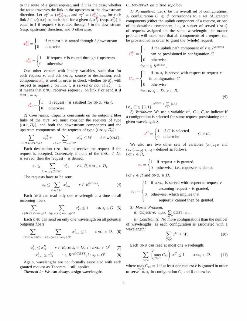
to the route of a given request, and if it is the case, whetherthe route traverses the link in the upstream or the downstreamdirection. LetxD
ℓ = (xDrℓ)r∈R and xD
ℓ = (xUrℓ)r∈R, for each
link ℓ ∈ ω(OLT) be such that, for a givenℓ, xDrℓ (resp.xU
rℓ) isequal to 1 if requestr is routed throughℓ in the downstream(resp. upstream) direction, and 0 otherwise.
xDrℓ =
1 if requestr is routed throughℓ downstream
0 otherwise
xUrℓ =
1 if requestr is routed throughℓ upstream
0 otherwise
One other vectors with binary variables, such that foreach requestr, and echONUi, source or destination, eachcomponentxℓ
ri is used in order to check whetherONUℓi , with
respect to requestr on link ℓ, is served or not. Ifxℓri = 1,
it means thatONUi receives requestr on link ℓ or send it ifONUi = sr.
xℓri =
1 if requestr is satisfied forONUi via ℓ.
0 otherwise
2) Constraints:Capacity constraints on the outgoing fiberlinks of the OLT: we must consider the requests of type(OLT, Dr), and both the downstream components and theupstream components of the requests of type(ONUi, Dr):
∑
r∈R:Dr∩Oℓ 6=∅
xDrℓ +
∑
r∈RACCESS:sr∈Oℓ
xUrℓ ≤ W ℓ ∈ ω(OLT).
Each destinationONU has to receive the request if therequest is accepted. Conversely, if none of theONUi ∈ Dr
is served, then the requestr is denied.
xr ≤∑
ℓ:ONUi∈Oℓ∩Dr
xℓri r ∈ R, ONUi ∈ Dr.
The requests have to be sent:
xr ≤∑
ℓ:sr∈Oℓ
xℓrsr
r ∈ RACCESS. (4)
Each ONU can read only one wavelength at a time on allincoming fibers:
∑
r∈R:Dr∩ONUi 6=∅
∑
ℓ∈ω(OLT):ONUi∈Oℓ
xℓri ≤ 1 ONUi ∈ O. (5)
EachONU can send on only one wavelength on all potentialoutgoing fibers:
∑
r∈R:sr=ONUi
∑
ℓ∈ω(OLT):ONUi∈Oℓ
xℓrsr
≤ 1 ONUi ∈ O. (6)
xℓri ≤ xD
rℓ r ∈ R, ONUi ∈ Dr, l : ONUi ∈ Oℓ (7)
xℓrsr
≤ xUrℓ r ∈ RACCESS, l : sr ∈ Oℓ (8)
Again, wavelengths are not formally associated with eachgranted request as Theorem 1 still applies.
Theorem 2:We can always assign wavelengths
C. MC-GRWA on a Tree Topology
1) Parameters:Let C be the overall set of configurations.A configuration C ∈ C corresponds to a set of grantedcomponents (either the uplink component of a request, or oneof its downlink component, i.e., a subset of servedONUs)of requests assigned on the same wavelength: the masterproblem will make sure that all components of a request canbe provisioned in order to grant the (whole) request.
CUr =
1 if the uplink path component ofr ∈ RACCESS
can be provisioned in configurationC
0 otherwise
for r ∈ RACCESS,
Cri =
1 if ONUi is served with respect to requestr
in configurationC
0 otherwise
for ONUi ∈ Dr, r ∈ R,
(9)
i.e., C ∈ 0, 1|RACCESS|+
P
r∈R
|Dr|.
2) Variables: We use a variablexC , C ∈ C, to indicate ifa configuration is selected for some request provisioning onagiven wavelengthλ.
xC =
1 if C is selected
0 otherwiseC ∈ C.
We also use two other sets of variables(xr)r∈R and(xri)ONUi∈Dr,r∈R defined as follows:For r ∈ R,
xr =
1 if requestr is granted,
0 otherwise, i.e., requestr is denied.
For r ∈ R and ONUi ∈ Dr,
xri =
1 if ONUi is served with respect to requestr
assuming requestr is granted,
0 otherwise, which implies that
requestr cannot then be granted.
3) Master Problem:a) Objective: max
∑
r∈R
COSTr xr .
b) Constraints:No more configurations than the numberof wavelengths, as each configuration is associated with awavelength:
∑
C∈C
xC ≤ W. (10)
EachONU can read at most one wavelength:
∑
C∈C
(
maxr∈R
Cri
)
xC ≤ 1 ONUi ∈ O. (11)
wheremaxr∈R
Cri = 1 if at least one requestr is granted in order
to serveONUi in configurationC, and 0 otherwise.
4

EachONU can send its requests on at most one wavelength:∑
C∈C
(
maxr∈RACCESS:sr=ONUi
CUr
)
xC ≤ 1 ONUi ∈ O (12)
where maxr∈RACCESS
CUr = 1 if at least one requestr ∈ RACCESS such
that sr = ONUi is granted in configurationC and thereforeuses the signal emitted atONUi, and 0 otherwise.
In order for a request to be granted, all of itsONU mustbe served, possibly with a different configuration (i.e., wave-length):
∑
C∈C
Cri xC ≥ xri ONUi ∈ Dr, r ∈ R (13)
xr ≤ xri ONUi ∈ Dr, r ∈ R (14)∑
C∈C
CUr xC ≥ xr r ∈ RACCESS. (15)
Let us first consider a requestr ∈ RCORE. Requestr can begranted if and only if all its destinations can be served, i.e.,xr = 1 if and only if xir = 1 for all ONUi ∈ Dr. Note that ifat least oneONUi ∈ Dr is not served (xir = 0), then, using(14) r cannot be granted (i.e.,xr = 0). In addition,xri = 1only if there is at least one selected configurationC (i.e., suchthat xC = 1) such thatCir = 1, see equation (13). On theother hand, if, for a givenr, all xri for i : ONUi ∈ Dr areequal to 1,xr will be set to 1 due to the fact that the objectiveis max
∑
r∈R
COSTrxr.
Let us next consider a requestr ∈ RACCESS. Requestr canbe granted if and only if(i) all its destinations can be servedand(ii) its uplink component can be provisioned, i.e.,xr = 1if and only if (i) xir = 1 for all ONUi ∈ Dr and(ii) there is atleast one selected configurationC (i.e., such thatxC = 1) suchthatCU
r = 1. Note that if either oneONUi ∈ Dr is not served(xir = 0) or the uplink component cannot be provisioned (i.e.,all selected configurationsC are such thatCU
r = 0), using (14)or (15),r cannot be granted (i.e.,xr = 0). On the other hand,if, for a given r, all xri for i : ONUi ∈ Dr are equal to 1and there is at least one selected configurationC such thatCU
r = 1, xr will be set to 1 due to the fact that the objectiveis max
∑
r∈R
COSTrxr.
4) Pricing Problem:a) Objective: Each pricing problem corresponds to the
generation of a configuration. The objective is to maximizethe reduced cost, i.e.,cC , or c for short, where
c = −u0 −∑
i:ONUi∈O
uDi
(
maxr∈R
Cri
)
−∑
i:ONUi∈O
uUi
(
maxr∈RACCESS:sr=ONUi
CUr
)
+∑
r∈R
∑
i:ONUi∈Dr
vDriCri +
∑
r∈RACCESS
vUr CU
r
whereu0 is the dual variable associated with constraint (10),uD
i ≥ 0 with (11), uUi ≥ 0 with (12), vD
ri ≤ 0 with (13), andvU
r ≤ 0 with (15).
In order to eliminate the nonlinearities, let us introduce thetwo binary variablesCD
i andCUi . In order to have:
CDi = max
r∈RCri (16)
CUi = max
r∈RACCESS:sr=ONUi
CUr (17)
we add the constraints :
CDi ≥ Cri r ∈ R, ONUi ∈ Dr (18)
CUi ≥ CU
r r ∈ RACCESS, i : ONUi = sr,
(19)
CDi ≤
∑
r∈R
Cri i : ONUi ∈ Dr, r ∈ R (20)
CUi ≤
∑
r∈RACCESS:ONUi=sr
CUr r ∈ RACCESS, i : ONUi = sr.
(21)
for i : ONUi ∈ O. Observe thatCDi = 1 if and only if ONUi
is served for at least one request, and 0 otherwise, and thatCU
i = 1 if and only if the path(ONUi, OLT) is provisioned forat least one request originating atONUi, and 0 otherwise.
The objective of the pricing problem can then be rewritten:
c = −u0 −∑
i:ONUi∈O
uDi CD
i −∑
i:ONUi∈O
uUi CU
i
+∑
r∈R
∑
i:ONUi∈Dr
vDriCri +
∑
r∈RACCESS
vUr CU
r .
b) Variables: We use two decision vectorsyD and yU
such that each componentyDℓ (resp. yU
ℓ ) indicates whetherthe wavelength associated with the configuration is useddownstream (resp. upstream) or not:yD
ℓ gets value 1 if itused downstream, 0 otherwise (i.e., it is either unused or usedupstream);yD
ℓ gets value 1 if it used upstream, 0 otherwise(i.e., it is either unused or used downstream).
yUℓ =
1 if the wavelength associated with the configuration
is used downstream onℓ
0 otherwise
yDℓ =
1 if the wavelength associated with the configuration
is used downstream onℓ
0 otherwise
Decision vectorC with components defined as in III-C.
CUr =
1 if the uplink path component ofr ∈ RACCESS
can be provisioned in configurationC
0 otherwise
for r ∈ RACCESS,
Cri =
1 if ONUi is served with respect to requestr
in configurationC
0 otherwise
for ONUi ∈ Dr, r ∈ R.
5
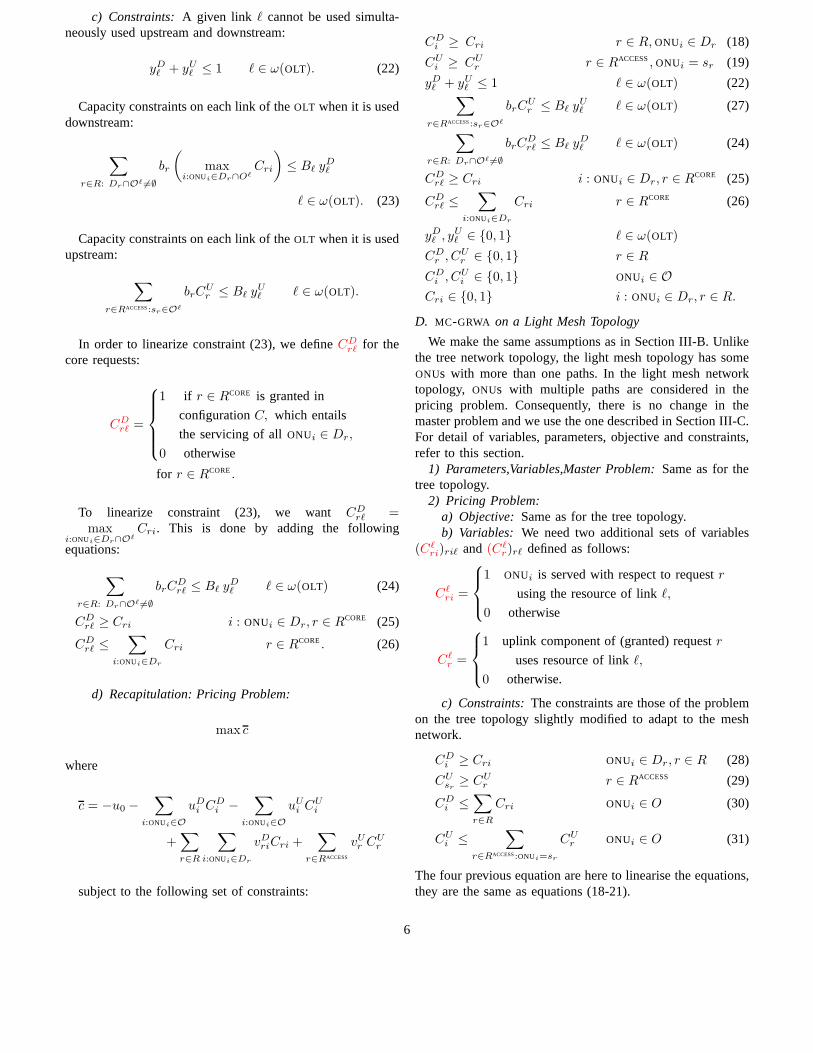
c) Constraints: A given link ℓ cannot be used simulta-neously used upstream and downstream:
yDℓ + yU
ℓ ≤ 1 ℓ ∈ ω(OLT). (22)
Capacity constraints on each link of theOLT when it is useddownstream:
∑
r∈R: Dr∩Oℓ 6=∅
br
(
maxi:ONUi∈Dr∩Oℓ
Cri
)
≤ Bℓ yDℓ
ℓ ∈ ω(OLT). (23)
Capacity constraints on each link of theOLT when it is usedupstream:
∑
r∈RACCESS:sr∈Oℓ
brCUr ≤ Bℓ yU
ℓ ℓ ∈ ω(OLT).
In order to linearize constraint (23), we defineCDrℓ for the
core requests:
CDrℓ =
1 if r ∈ RCORE is granted in
configurationC, which entails
the servicing of allONUi ∈ Dr,
0 otherwise
for r ∈ RCORE.
To linearize constraint (23), we wantCDrℓ =
maxi:ONUi∈Dr∩Oℓ
Cri. This is done by adding the following
equations:
∑
r∈R: Dr∩Oℓ 6=∅
brCDrℓ ≤ Bℓ yD
ℓ ℓ ∈ ω(OLT) (24)
CDrℓ ≥ Cri i : ONUi ∈ Dr, r ∈ RCORE (25)
CDrℓ ≤
∑
i:ONUi∈Dr
Cri r ∈ RCORE. (26)
d) Recapitulation: Pricing Problem:
max c
where
c = −u0 −∑
i:ONUi∈O
uDi CD
i −∑
i:ONUi∈O
uUi CU
i
+∑
r∈R
∑
i:ONUi∈Dr
vDriCri +
∑
r∈RACCESS
vUr CU
r
subject to the following set of constraints:
CDi ≥ Cri r ∈ R, ONUi ∈ Dr (18)
CUi ≥ CU
r r ∈ RACCESS, ONUi = sr (19)
yDℓ + yU
ℓ ≤ 1 ℓ ∈ ω(OLT) (22)∑
r∈RACCESS:sr∈Oℓ
brCUr ≤ Bℓ yU
ℓ ℓ ∈ ω(OLT) (27)
∑
r∈R: Dr∩Oℓ 6=∅
brCDrℓ ≤ Bℓ yD
ℓ ℓ ∈ ω(OLT) (24)
CDrℓ ≥ Cri i : ONUi ∈ Dr, r ∈ RCORE (25)
CDrℓ ≤
∑
i:ONUi∈Dr
Cri r ∈ RCORE (26)
yDℓ , yU
ℓ ∈ 0, 1 ℓ ∈ ω(OLT)
CDr , CU
r ∈ 0, 1 r ∈ R
CDi , CU
i ∈ 0, 1 ONUi ∈ O
Cri ∈ 0, 1 i : ONUi ∈ Dr, r ∈ R.
D. MC-GRWA on a Light Mesh Topology
We make the same assumptions as in Section III-B. Unlikethe tree network topology, the light mesh topology has someONUs with more than one paths. In the light mesh networktopology, ONUs with multiple paths are considered in thepricing problem. Consequently, there is no change in themaster problem and we use the one described in Section III-C.For detail of variables, parameters, objective and constraints,refer to this section.
1) Parameters,Variables,Master Problem:Same as for thetree topology.
2) Pricing Problem:a) Objective: Same as for the tree topology.b) Variables: We need two additional sets of variables
(Cℓri)riℓ and (Cℓ
r)rℓ defined as follows:
Cℓri =
1 ONUi is served with respect to requestr
using the resource of linkℓ,
0 otherwise
Cℓr =
1 uplink component of (granted) requestr
uses resource of linkℓ,
0 otherwise.
c) Constraints:The constraints are those of the problemon the tree topology slightly modified to adapt to the meshnetwork.
CDi ≥ Cri ONUi ∈ Dr, r ∈ R (28)
CUsr
≥ CUr r ∈ RACCESS (29)
CDi ≤
∑
r∈R
Cri ONUi ∈ O (30)
CUi ≤
∑
r∈RACCESS:ONUi=sr
CUr ONUi ∈ O (31)
The four previous equation are here to linearise the equations,they are the same as equations (18-21).
6

The following equations are specific to the mesh topology.They express the possibility to serve anONU using differentfibersℓ.
Cℓri ≤ Cri ONUi ∈ Dr, ℓ : ONUi ∈ Oℓ, r ∈ R (32)
Cℓr ≤ CU
r r ∈ RACCESS, ℓ : sr ∈ Oℓ (33)
Cri ≤∑
ℓ:ONUi∈Oℓ
Cℓri ONUi ∈ Dr, r ∈ R (34)
CUr ≤
∑
ℓ:sr∈Oℓ
Cℓr r ∈ RACCESS (35)
Then we have equations to verify that no fibers and nowavelength are over-used :
yDℓ + yU
ℓ ≤ 1 ℓ ∈ ω(OLT) (36)∑
r∈R
brCℓri ≤ Bℓy
Dℓ ℓ ∈ ω(OLT) (37)
∑
r∈RACCESS:sr∈Oℓ
brCℓr ≤ Bℓy
Uℓ ℓ ∈ ω(OLT) (38)
Finally, the following equations allow to determine whichONU receives which request in the configuration we arecomputing.
Clri ≤ CD
rℓ r ∈ R, ONUi ∈ Dr, l : ONUi ∈ Ol (39)
Clr ≤ CU
rℓ r ∈ R, l : sr ∈ Ol (40)
∑
ℓ:ONUi∈Oℓ
Cℓri ≤ 1 ONUi ∈ Dr, r ∈ R (41)
∑
ℓ:sr∈Oℓ
Cℓr ≤ 1 r ∈ RACCESS (42)
IV. M AXIMIZING THE NUMBER OF SERVED ONUS
In this section, we define the mathematical models forthe tree and the light mesh topologies with/without trafficc-grooming, where the objective is to maximize the weightednumber of servedONUs subject to the available resources inthe networks. A partially granted request is defined as a requestthat is granted to serve a few (at least one) destinationONUs.In this section, while maximizing the number of servedONUswe may grant partially requests and/or whole requests. In aweighted version, we can associate a cost to each servedONU
that would represent weight ofONU.
A. MC-RWA on WDM-PON Tree Topology
A new optimization model for the tree network with-out traffic-grooming, with the objective of maximizing theweighted number of servedONUs, is proposed as follows.
1) Objective: We need the variablesxri, which for eachrequestr and eachONU, destination or source ofr, indicatesif r is satisfied for thisONU.
xri =
1 if requestr is satisfied forONUi
0 otherwise
The objective is to maximize the number of servedONUs:
max∑
r∈R
∑
i:ONUi∈Dr
COSTrixri.
whereCOSTriis the cost associated withONUi with respect
to request r.2) Constraints: We use the same variables as in previous
formulation, exeptxr which is replaced byxℓr. It indicates if
requestr is sent on fiberℓ or not.
xr =
1 if requestr is granted
0 otherwise
Capacity constraints on the fiber link of theOLT: Upstream& downstream wavelengths of theONUs can’t be exceeds fromavailable wavelength on each associated link.xℓ
r gets value 1if requestr is served on linkℓ, 0 otherwise.
xℓr =
1 if requestr is granted on linkℓ
0 otherwise
∑
r∈R:Dr∩Oℓ 6=∅
xℓr +
∑
r∈RACCESS:sr∈Oℓ
xℓr ≤ W ℓ ∈ ω(OLT).
(43)EachONU can read only one wavelength:
∑
r∈R:ONUi∈Dr
xri ≤ 1 ONUi ∈ O. (44)
EachONU can send only one wavelength:∑
r∈RACCESS:ONUi=sr
xri ≤ 1 ONUi ∈ O. (45)
In order to grant the requestr on link ℓ, at least oneONU
in the destination of requestr in Oℓ must be accepted:
xℓr ≤
∑
i:ONUi∈Dr∩Oℓ
xri r ∈ R, l ∈ ω(OLT). (46)
In order to grant the requestr, sourceONU (if it is notOLT) of requestr must be accepted:
xℓr ≤ xrsr
r ∈ RACCESS, l ∈ ω(OLT). (47)
The requestr must be granted in order to grant the desti-nation ONU(s) : If none of theONUi is served, thexr denied
xℓr ≥ xri ℓ ∈ ω(OLT), ONUi ∈ Dr ∩ Oℓ. (48)
B. MC-RWA on WDM-PON Light Mesh Topology
This section describes theMC-RWA (without traffic-grooming) problem onWDM-PON light mesh network topol-ogy with the objective of maximizing the weighted number ofservedONUs.
1) Objective: Maximize the number of servedONUs:
max∑
r∈R
∑
i:ONUi∈Dr
∑
ℓ:ONUi∈Oℓ
COSTrixℓri
7

2) Constraints: Concerning the capacity of the opticalfibers, it has a limited number of wavelengths and we cannot exceed this number of available wavelengths on each link.Note that, as before, wavelengths are bidirectional, so they canbe use either for downstream or upstream direction and that weassume that we are free to use the wavelengths downstreamand upstream. The following set of constraints assures thatwavelengths used in the downstream and upstream directiondo no exceed the total number of available wavelength on eachlink outgoing theOLT. First recall the variables that are used:
xDrℓ =
1 if requestr is routed throughℓ downstream
0 otherwise
xUrℓ =
1 if requestr is routed throughℓ upstream
0 otherwise
xℓri =
1 if requestr is satisfied forONUi via ℓ.
0 otherwise
xr =
1 if requestr is granted
0 otherwise
∑
r∈R:Dr∩Oℓ 6=∅
xDrℓ +
∑
r∈RACCESS:sr∈Oℓ
xUrℓ ≤ W
ℓ ∈ ω(OLT). (49)
EachONU can read only one wavelength:∑
r∈R:ONUi∈Dr
∑
ℓ:ONUi∈Oℓ
xℓri ≤ 1 ONUi ∈ O. (50)
EachONU can send only on one wavelength:∑
r∈RACCESS
∑
ℓ:sr∈Oℓ
xℓrsr
≤ 1 sr ∈ O. (51)
In order to grant the requestr, at least oneONU in thedestination of requestr must be accepted:
xr ≥∑
ℓ:ONUi∈Oℓ
xℓri ONUi ∈ Dr, r ∈ R. (52)
In order to grant the requestr, SourceONU (if it is not OLT)of requestr must be accepted:
xr ≤∑
ℓ:sr∈Oℓ
xℓrsr
r ∈ RACCESS. (53)
If none of theONUi is served, thexr denied:
xr ≤∑
i:ONUi∈Dr
∑
ℓ:ONUi∈Oℓ
xℓri r ∈ R. (54)
If link ℓ accepts the requestr for downstream, then all thedestinationONU(s) of r on ℓ can be accepted:
xDrℓ ≤
∑
i:ONUi∈Oℓ
xℓri r ∈ R, ONUi ∈ Dr ∩Oℓ. (55)
If link ℓ accepts the requestr for upstream, then sourceONU of r on ℓ can be accepted:
xUrℓ ≤ xℓ
rsrr ∈ RACCESS, ℓ : sr ∈ Oℓ. (56)
If link ℓ accepts the requestr for downstream, then desti-nation ONUi of r on ℓ can be accepted:
xDrℓ ≥ xℓ
ri r ∈ R, ℓ : ONUi ∈ Dr ∩ Oℓ. (57)
C. MC-GRWA on a Tree Topology
1) Master Problem:The master problem is quite similar tothe one we discussed in Section III-D, except that, now, ourobjective is to maximize the weighted number of destinationONUs. In this problem, the parameter vector has as componentsCri and Cr for ONUi ∈ Dr, r ∈ R and the variable vectorsarexC , xri as defined in Section III-C and IV-A.
xC =
1 if C is selected
0 otherwiseC ∈ C.
xri =
1 if requestr is satisfied forONUi
0 otherwise
Note that, in this problem we do not use the vector withcomponentsxr, instead, we use a new vector whose compo-nents arexsr
, defined as follows:
xsr=
1 if sourcesr = ONUi of a requestr is served in
the upstream direction, forr ∈ RACCESS
0 otherwise
a) Objective:
max∑
r∈R
COSTrixri.
b) Constraints: We have the same capacity constraintsas in III-C, Equations (10-12).
In order to serve destinationONUi with respect to requestrin the downstream direction,one of its associated configurationC must be granted, this is Equation 13. Equation 13 deals withthe upstream direction.
We also need the two equations:
xri ≤ xsrONUi ∈ Dr, r ∈ RACCESS (58)
xsr≤
∑
ONUi∈Dr
xrir ∈ RACCESS (59)
2) Pricing Problem: The pricing problem is same as thepricing problem for the tree when the objective is to maximizethe weighted number of granted requests in Section III-C. Asmentioned previously, the number of granted requests/ONUsare considered in the master problem and the configuration isgenerated by the pricing problem, so that there is no changein the pricing problem while generating the configurationC.Consequently, the pricing problem has same reduced costobjective as well as constrains and descriptions of their pa-rameters, variables.
8
D. MC-GRWA on a Mesh Topology
The light mesh traffic-grooming model, like other traffic-grooming models, is divided into two subproblems called mas-ter problem and pricing problem, discussed in the followingsections. The characterisitic of a configurationC are thosedescribed in Section III-D.
1) Master Problem:The master problem is the same thanthe master problem for the tree network topology, describedinSection IV-C, with the same objective. The difference is thatin a light mesh network, a few or allONUs have multiple pathsto the OLT. This multiple paths constraints are considered inthe pricing problem.
2) Pricing Problem: Similarly, the pricing problem is thesame as the pricing problem for the light mesh network topol-ogy with the objective of maximizing the weighted numberof granted requests, presented in Section III-D. As mentionedpreviously, the pricing problem provide a configuration to themaster problem, which selects them. There is no change in thepricing problem.
V. SOLUTIONS OF THE MC-RWA MODELS
A. An Overview on Column Generation Modeling
Column generation techniques offer solution methods forlinear programs with a very large number of variables (e.g.,exponential) where constraints can be expressed implicitly.They rely on a decomposition of the initial linear programinto themaster problemand thepricing problem. The masterproblem corresponds to a linear program associated with arestricted constraint matrix, with respect to the number ofvariables (or columns) of the initial constraint matrix. Thepricing problem is defined by the optimization of the so-called reduced cost (refer to [1] if not familiar with linearprograming) subject to the implicit constraints expressedbythe coefficients of the constraint matrix of the master problem.
The column generation solution scheme is similar to thatof the simplex algorithm: it is an iterative process where, ateach step, we attempt to add one or more columns to theconstraint matrix of the master problem in order to improve thevalue of its objective function. The search for such columnsis made through the solution of the pricing problem. If itsoutcome corresponds to one or more columns with a negativereduced cost (assuming we deal with minimization), then itentails an improvement of the value of the master objectivefunction; otherwise, if no solution of the pricing problem canbe identified with a negative cost, we then conclude that thecurrent solution is indeed optimal.
Column generation can be combined with branch-and-bound techniques for solving integer linear programs witha large number of variables, see [2] for a nice overview.Branching rules have to be devised properly in order to avoidgenerating a huge number of subproblems in the search treeassociated with the branch-and-bound, either by branchingon the variables of the master problem using cuts, or bybranching on the variables of the pricing problem usingclassical branching schemes or cuts.
B. Solution of theMC-RWA and MC-GRWA Models
First we solve the linear relaxation using a column gen-eration method where the master problem is solved usingthe LP CPLEX package, and where the pricing problemsare solved using the ILP CPLEX package. Once we haveobtained the optimal solution of the LP relaxation, we use theILP CPLEX package again in order to get an ILP solutionfor the master problem. This does not lead necessarily toan optimal solution of the corresponding MC-RWA and MC-GRWA model. However, bounds can be obtained on the qualityof the ILP solution obtained this way. Moreover, in order tospeed the process of getting an ILP solution for the masterproblems, we also use a rounding off procedure that works asfollows.Objective 2: Maximizing the number of servedONUs.Consider the configuration which contributes the most tosatisfying ONUs and such thatxλ
C is fractional.Round offxλ
C to 1.Re-optimize the LP relaxation assumingxλ
C = 1.Reiterate.
VI. COMPUTATIONAL RESULTS
We plan simulations for both theMC-RWA and theMC-GRWA problems on tree and mesh topologies which aredescribed in next section. These experiments will be doneunder two different scenarios as described in the last section.
1) Network Instances:We consider a network with a singleOLT and eight outgoing bidirectional fibers. For each fiberℓ,there is 32ONUs (leaf nodes independently of the tree or meshstructure). Each fiber have height or sixteen wavelengths.
2) Traffic Instances:In the first scenario, we simply con-siderOLT-ONUs requests while in the second one we considerboth OLT-ONUs andONU-ONUs requests. When grooming isnot considered, we assume that each request use 100% of thecapacity of a wavelength, otherwise it is specified accordingto the type of the request. Here is the description of the twoscenarios we consider.
a) First scenario.: There is three types of requests:requests corresponding to customers viewing video or TV.They represent 60% of the requests and each request usebetween 50 and 90% of the bandwidthB available in awavelength. These requests are multicast requests with 1 to5destinations. The second type of requests corresponds to radiotransmission. We suppose that it represent 20% of the trafficand that each request use from 20 to 50% of the bandwith ofa wavelength. The third request corresponds to users surfingon the net. It represents 20% of the requests and they use only10% of the available bandwith.
b) Second scenario.:There is a fourth type of requests:It correspond to neighbors playing together on-line games.It is represented by a multicast originating at anONU withdestination set of size from 4 to 10. The request use from 30to 60% of the bandwith of a wavelength. This type of requestrepesent 50% of the requests in the second scenario. In thisscenario, the proportion of the three previous types of requestsare respectively 30%, 10% and 10%.
9

A. Evaluation Parameters
We want to compare the two objectives different objectives:
• maximizing the grade of service• maximizing the number of granted ONUs
We will compare the bandwidth usage and the wastedbandwidth.
VII. C ONCLUSIONS
An interesting evolution is to consider a mix of bothobjectives: we should require some request to be fully satisfiedn order to be counted in the objective, while for other requesteach servedONU will be counted independantly.
ACKNOWLEDGMENT
Work of B. Jaumard has been supported by a Concordia Re-search Chair on the Optimization of Communication Networksand by a NSERC grant. Work of D. Coudert has been partiallysupported by ANR-JC OSERA, INRIA, European project ISTFET AEOLUS, COST 293 and Region Provence Alpes Coted’Azur PACA. The research done is in this paper was initiatedduring visits of B. Jaumard and D. Coudert in France andQuebec, supported by a FQRNT-INRIA grant.
REFERENCES
[1] M. Maier, M. Herzog, and M. Reisslein, “STARGATE: The Next Evo-lutionary Step toward Unleashing the Potential of WDM EPONs,” IEEECOMMUNICATIONS MAGAZINE, vol. 45, no. 5, p. 50, 2007.
[2] C. Barnhart, E. Johnson, G. Nemhauser, M. Savelsbergh, and P. Vance,“Branch-and-Price: Column Generation for Solving Huge Integer Pro-grams,” OPERATIONSRESEARCH-BALTIMORE-, vol. 46, pp. 316–329, 1998.
10

258 Annexes

Annexe D
Fiabilité et tolérance aux pannes
D.1 Reliability of Connections in Multilayer Networks un-der Shared Risk Groups and Costs Constraints
Article présenté lors d’ICC08.
D.2 Overlapping Segment for an Efficient Protection ofWDM Networks
Article en préparation.
259
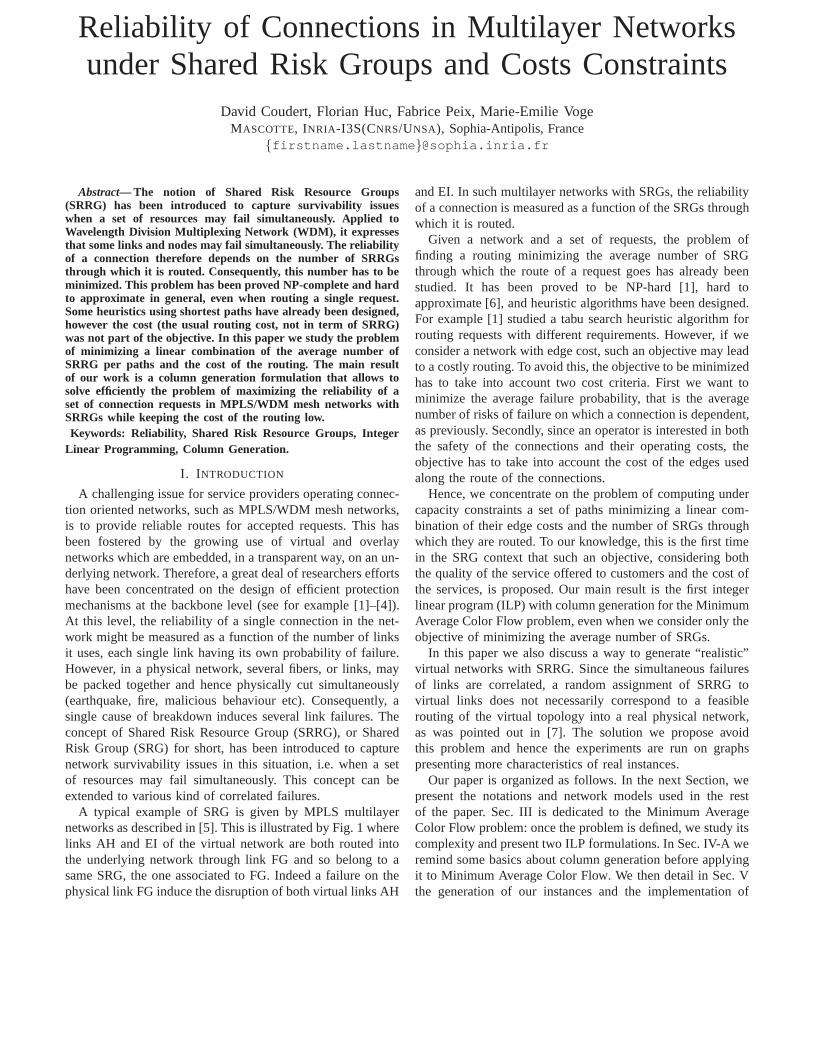
Reliability of Connections in Multilayer Networksunder Shared Risk Groups and Costs Constraints
David Coudert, Florian Huc, Fabrice Peix, Marie-Emilie VogeMASCOTTE, INRIA-I3S(CNRS/UNSA), Sophia-Antipolis, France
Abstract— The notion of Shared Risk Resource Groups(SRRG) has been introduced to capture survivability issueswhen a set of resources may fail simultaneously. Applied toWavelength Division Multiplexing Network (WDM), it expressesthat some links and nodes may fail simultaneously. The reliabilityof a connection therefore depends on the number of SRRGsthrough which it is routed. Consequently, this number has tobeminimized. This problem has been proved NP-complete and hardto approximate in general, even when routing a single request.Some heuristics using shortest paths have already been designed,however the cost (the usual routing cost, not in term of SRRG)was not part of the objective. In this paper we study the problemof minimizing a linear combination of the average number ofSRRG per paths and the cost of the routing. The main resultof our work is a column generation formulation that allows tosolve efficiently the problem of maximizing the reliability of aset of connection requests in MPLS/WDM mesh networks withSRRGs while keeping the cost of the routing low.Keywords: Reliability, Shared Risk Resource Groups, Integer
Linear Programming, Column Generation.
I. I NTRODUCTION
A challenging issue for service providers operating connec-tion oriented networks, such as MPLS/WDM mesh networks,is to provide reliable routes for accepted requests. This hasbeen fostered by the growing use of virtual and overlaynetworks which are embedded, in a transparent way, on an un-derlying network. Therefore, a great deal of researchers effortshave been concentrated on the design of efficient protectionmechanisms at the backbone level (see for example [1]–[4]).At this level, the reliability of a single connection in the net-work might be measured as a function of the number of linksit uses, each single link having its own probability of failure.However, in a physical network, several fibers, or links, maybe packed together and hence physically cut simultaneously(earthquake, fire, malicious behaviour etc). Consequently, asingle cause of breakdown induces several link failures. Theconcept of Shared Risk Resource Group (SRRG), or SharedRisk Group (SRG) for short, has been introduced to capturenetwork survivability issues in this situation, i.e. when asetof resources may fail simultaneously. This concept can beextended to various kind of correlated failures.
A typical example of SRG is given by MPLS multilayernetworks as described in [5]. This is illustrated by Fig. 1 wherelinks AH and EI of the virtual network are both routed intothe underlying network through link FG and so belong to asame SRG, the one associated to FG. Indeed a failure on thephysical link FG induce the disruption of both virtual linksAH
and EI. In such multilayer networks with SRGs, the reliabilityof a connection is measured as a function of the SRGs throughwhich it is routed.
Given a network and a set of requests, the problem offinding a routing minimizing the average number of SRGthrough which the route of a request goes has already beenstudied. It has been proved to be NP-hard [1], hard toapproximate [6], and heuristic algorithms have been designed.For example [1] studied a tabu search heuristic algorithm forrouting requests with different requirements. However, ifweconsider a network with edge cost, such an objective may leadto a costly routing. To avoid this, the objective to be minimizedhas to take into account two cost criteria. First we want tominimize the average failure probability, that is the averagenumber of risks of failure on which a connection is dependent,as previously. Secondly, since an operator is interested inboththe safety of the connections and their operating costs, theobjective has to take into account the cost of the edges usedalong the route of the connections.
Hence, we concentrate on the problem of computing undercapacity constraints a set of paths minimizing a linear com-bination of their edge costs and the number of SRGs throughwhich they are routed. To our knowledge, this is the first timein the SRG context that such an objective, considering boththe quality of the service offered to customers and the cost ofthe services, is proposed. Our main result is the first integerlinear program (ILP) with column generation for the MinimumAverage Color Flow problem, even when we consider only theobjective of minimizing the average number of SRGs.
In this paper we also discuss a way to generate “realistic”virtual networks with SRRG. Since the simultaneous failuresof links are correlated, a random assignment of SRRG tovirtual links does not necessarily correspond to a feasiblerouting of the virtual topology into a real physical network,as was pointed out in [7]. The solution we propose avoidthis problem and hence the experiments are run on graphspresenting more characteristics of real instances.
Our paper is organized as follows. In the next Section, wepresent the notations and network models used in the restof the paper. Sec. III is dedicated to the Minimum AverageColor Flow problem: once the problem is defined, we study itscomplexity and present two ILP formulations. In Sec. IV-A weremind some basics about column generation before applyingit to Minimum Average Color Flow. We then detail in Sec. Vthe generation of our instances and the implementation of

A B D
H
E IF
E
A
G
H
B C D
IF
underlyingnetwork
virtualnetwork
Fig. 1. Example of SRLG: virtual links AH and EI share the samerisk FG.
our solving process, and finally we analyze the computationalresults before concluding.
II. N ETWORK MODEL AND NOTATIONS
The multilayer networks we consider are composed of twolayers, a physical or underlying network and a virtual one.
The physical layer is modelled by a digraphGPN =(VPN, LPN), where VPN is the set of nodes, andLPN =e1, . . . em is the set of links (i.e. unidirectional fibers).Similarly, the virtual network embedded in the physical oneis modelled by the digraphGVN = (VVN, LVN). Each arce ∈ LVN has a costγe per flow unit and a capacityue. Theconstruction of the virtual networks used in our simulationswill be described more precisely in Sec. V.
Each arcei of the physical networkGPN gives in the virtuallayer of a single risk group that we represent by a colorci.More precisely, colorci is the subset of arcs of the virtualnetwork routed through arcei on the underlying layer, thatis the set of arcs sharing the risk of failure of arcei. The setC = c1, . . . , cm is the set of colors (i.e. SRG) of the network.Note at that point that an arc of the virtual network may belongto several SRGs (= colors). However, following [1], [2], [5],we apply the simple transformation onGVN described in [6],[8] : each multi-colored arc is replaced with a chain of mono-colored arcs, so that each arc now belongs to exactly onecolor. For simplicity purpose we will denote also byGVN themodified graph. Such graphs with SRG are refered to in theliterature ascolored graphs. Interested readers may refer to [9]for a model with multiple colors per edges, and to [8] for apreliminary comparison of both models.
Let K be a set of connection requests overGVN, suchthat for each requestk ∈ K, we are given its sourcesk, itsdestinationtk and its integral bandwidth requirementdk. Weassume that each request can be split into unitary requests tobe served independently. Consequently, in the rest of the paperall the requests are unitary. For each requestk ∈ K, Pk is theset of all thesktk-directed paths inGVN andP = ∪k∈KPk
Finally, we denote respectively byΓ−(v) andΓ+(v) the setof incoming and outgoing links at a nodev.
III. M INIMUM AVERAGE COLOR FLOW PROBLEM
(MACF)
A. Problem definition
An instance of the Minimum Average Color Flow problemconsists in a digraphGVN = (VVN, LVN), representing the
virtual network, with arc costγe per flow unit and capacityue for each arce ∈ LVN. A set C = c1, . . . , cm of colors-or SRG- partitioning the arc setLVN is given, as well as aset of unitary connection requestsK and a realα ∈ [0, 1].
A solution is a routing of all the requests satisfying all thecapacity constraints.
The objective to be minimized is a convex combinationof two cost criteria whose respective contributions can beadjusted through the parameterα ∈ [0, 1]. The first crite-rion, related to the operating cost, is the classical flow costdepending on the arc costsγe divided by the total flowrequest (= |K|). The second criterion, related to the safetyof the connections, is the average number of colors - SRGs- to which belongs a path routing one unit of flow, thatis the sum of the numbers of colors on which is routedeach request divided by|K|. The objective function is thenα|K| × (classical flow cost)+ (1−α)
|K| × (SRG flow cost).Note that whenα = 0 the problem becomes the min-
imisation of the average number of SRG or in other wordthe average probability of failure for a connection, whereasif α = 1 the problem is reduced to a classical integralmulticommodity flow.
B. Complexity
We now study the complexity of MACF under varioushypothesis on the colored graph. We deduce these results forMACF from one of its subproblems: Minimum Color Pathwith Edge Costs problem (MCPwEC) which is the MACFproblem with a single request, i.e.|K| = 1, and unitary arccapacities. Thus, it consists in finding a path from a sources
to a sink t minimizing a convex combination of the numberof colors used by the path and of the classical path cost.
1) Null arc costs: With null arc costs, this problem isthe Minimum Color Path problem (MCP) which has beenproved NP-hard in [2] and hard to approximate within a factor
2log1−δ |C|12 in [6], with δ = (log log |C|
12 )−ε andε < 1
2 . Theseresults were proved for undirected graphs, but their adaptationto the directed case is straightforward and induces the samefactor for MACF.
2) Span 1: MCP can be solved in polynomial time whensome conditions are satisfied on thespanof the colors of thegraph [6], [8], [10]. The span of a color is the number ofconnected components in the subgraph induced by the edgesof that color. The influence of this parameter on the MCPcomplexity has been studied in [6], [11]. However, we showthat the span has no such an influence on the hardness ofMCPwEC.
Theorem 1: [6] When all colors have span 1, MCP ispolynomial.
The proof is based on the fact that within a connectedcomponent of a colorc, each vertex is reachable from anyother vertex of the component using only edges of colorc.
The span definition and Theorem 1 can easily be extendedto thecolor symmetric digraphsettings, i.e. when an arc andits reverse arc belong to the same color: the span is simply the
2

number of strongly connected components and the property isstill verified.
Let us now prove that the adjunction of edge costs deeplymodify the complexity properties of MCP since MCPwEC isas hard to approximate as in the general directed case in theaforesaid symmetric settings.
Theorem 2:The MCPwEC problem on a color symmetricdigraph is NP-hard and hard to approximate within a factor
2log1−δ |C|12 with δ = (log log |C|
12 )−ε and ε < 1
2 even whenall colors have span 1.
Proof: The proof is a reduction from MCP to MCPwEC.Let G be a color symmetric digraph on color setC withunspecified span and two verticess andt defining an instanceof MCP. We construct an instance of MCPwEC on the digraphG′ with convex coefficientα in the objective function.G′ isthe graphG with two additional symmetric arcs of colorc andcost X > 1−α
α|C| between each pair of strongly connected
components ofc. The cost of arcs fromG in G′ is null andall the capacities are unitary.
An optimalst-path for the MCPwEC instance uses none ofthe added arcs since using only ones costαX > (1 − α)|C|,which is greater than the cost of using the whole arc and colorsets ofG. Therefore, an optimal path inG′ for MCPwEC is anoptimal path inG for MCP too. Indeed the two costs of a samepath for MCPwEC and MCP differ only by the multiplicativeconstant1 − α. This last point concludes the proof.
From Theorem 2 we can deduce that in this special caseMACF is as hard to approximate as its subproblem MCPwEC.
3) Color reduced to a single arc:Unlike MCPwEC andMCP, MACF remains NP-hard and hard to approximate whenall colors are reduced to a single arc. Indeed in such a case,MCPwEC and MCP are merely polynomial shortest pathproblems while MACF still contains the Minimum Edge CostFlow problem (MECF) as a subproblem. The MECF problemconsists in routing a single integral request in a digraph withcapacities and fixed arc costs, that is the cost of using an arcis the same whatever the flow value is on it, as long as itis positive. This problem is NP-hard and hard approximatewithin a factor2log1−ε n, ∀ε > 0 [12].
Theorem 3:The MACF problem is hard to approximatewithin a factor≈ 2log1−ε n ∀ε > 0 even when all colors arereduced to a single arc, unlessNP ⊆ DTIME(npolylogn).
C. ILP Formulations
In this section we present two ILP formulations for MACFbased on the two classical multiflow formulations: the compactnode-arc formulation and the exponential size arc-path one(see [13]). Although exponential, the arc-path formulation ismore efficient than the compact one thanks to the possible useof column generation techniques.
1) Node-Arc Formulation:The binary flow variablezke for
e ∈ LVN andk ∈ K gets value 1 if the virtual linke is used toroute the unitary requestk and 0 otherwise. The binary colorvariableχc
k, for k ∈ K andc ∈ C, gets values 1 if the unitaryrequestk is routed through an arc belonging to the risk grouprepresented by colorc.
min1
|K|
∑
k∈K
(
α∑
c∈C
χck + (1 − α)
∑
e∈A
γezke
)
∑
e∈Γ+(v)
zke −
∑
e∈Γ−(v)
zke =
1 if v = sk
-1 if v = tk0 otherwise
∀k ∈ K (1)
∑
k∈K
zke ≤ ue ∀e ∈ LVN (2)
zke ≤ χ
c(e)k ∀k, ∀e ∈ LVN (3)
Constraints (1) and (2) are the classical flow conservationand capacity constraints of a node-arc multiflow formulation.Constraint (3) ensures that whenever the flow for a requestk
on an arce is positive, the colorc(e) of this arc is countedas used for this request, i.e. the value ofχ
c(e)k is forced to 1,
wherec(e) is the color of arce. There are|K|(|LVN| + |C|)variables and|K|(|VVN| + |LVN|) + |LVN| constraints.
The objective to be minimized is the average on all requestsof a convex combination of the number of colors used by arequest and of the classical cost of the route of a request.
2) Arc-Path Formulation:We now use binary variablezkp
which gets value 1 if the requestk ∈ K is routed on the pathp ∈ P , and 0 otherwise. As there might be a large number(exponential) of valid paths for each request, there might bea large number of variables in this family. As in the node-arcformulation, the binary variableχc
k has value1 if the pathused by requestk uses an arc of colorc and0 otherwise.
min1
|K|
∑
k
α∑
c∈C
χc(e)k + (1 − α)
∑
e∈LVN
∑
P∈Pk|e∈P
γezkP
∑
P∈Pk
zkP = 1 ∀k ∈ K (σk) (4)
∑
k
∑
P∈Pk|e∈P
zkP ≤ ue ∀e ∈ LVN (ωe) (5)
∑
P∈Pk|e∈P
zkP ≤ χ
c(e)k ∀k ∈ K, ∀e ∈ LVN (πk
e ) (6)
Constraints (4) ensure the satisfaction of all requests: for agiven requestk there must be a path used to route it; we callσk the associated dual variable. The capacity constraint (5) oneach arc expresses that there can not be more paths usingan arc e than there is bandwidth to fit them; we callωe
the associated dual variables. As in the node-arc formulation,constraints (6) take into account the colors used to serveeach request. The objective function is also similar. Thereare|K|(|LVN| + 1) + |LVN| constraints and empirically at most10|K| variables, which is a lot smaller (for both variables andconstraints) than in the node-arc formulation.
Note that to apply the column generation technique, or moreprecisely to define the auxiliary problem, we need the dualconstraint associated to the large size family of variableszk
p .
3

IV. SOLVING M INIMUM AVERAGE COLOR FLOW
A. Principle of column generation
A column generation formulation is a transformation of alinear program containing a very large size variable family(e.g., exponential) into two subproblems: themaster problemand theauxiliary problem. This decomposition relies on theDantzig-Wolf decomposition [13]. It allows to consider onlya subset of variables at a time.
Basically, starting with an initial reduced set of variables,we solve the master problem and obtain dual variable valuesthat will be used by the auxiliary problem. Then, we solvethe auxiliary problem to obtain new variables for the masterproblem, and so on. We repeat this loop until the auxiliaryproblem finds no more variables for the master problem. Thesolution of the master problem is then optimal (see [14]).
Column generation can be combined with branch-and-bound techniques to solve integral linear programs with a largenumber of variables, see [15] for a nice overview.
B. Column generation applied to MACF
1) Master Problem:The master problem corresponds to theoriginal arc-path formulation in which only a subset of thevariables from the large size familieszk
pp∈Pk is considered,all other variables of these families simply do not exist.
2) Auxiliary Problem: The auxiliary problem is deducedfrom the dual constraints of the master problem associated tothe large size family of variablezk
p :
σk ≤∑
e∈P
(
(1−α)|K| γe + ωe + πk
e
)
∀k, ∀P ∈ Pk
A solution of the auxiliary problem is a pathP violatingthis constraint. In our case the auxiliary problem is a shortestpath problem onGV N with arc cost(1−α)
|K| γe + ωe + πke . We
have to solve the auxiliary problem for each requestk. Noticethat the arc costs depend on the request, indeed thecolor cost(χc(e)
k ) is not the same for each request.3) Generation of the initial solution:The initial set of
variables of the master program has to contain the non nullvariables of a feasible solution otherwise the column genera-tion process can not start. To find this initial subset of variableswe solve a classical minimum cost multiflow problem: fromMACF we keep only the arc costs and capacities and we try tosatisfy all the requests under the capacity constraints (see [13]for references on the minimum cost multiflow problem).
C. Obtaining integral solutions: Branching
We first solve with column generation a relaxation of theproblem in which the variableszk
P and χck are fractional.
Then we do branching to obtain an integral solution. Duringthe branching a lot of computational time can be saved byconsidering theχc
k as fractional variables. Indeed, since allrequests are unitary, once the flow variables are integral, theconstraints force theχc
k variables to be integral too.
V. EXPERIMENTS
We have used CPLEX with a Concert Java interface and theopen sourceMASCOPT library [16] to implement our model.
A. Generation of instances
To give a realistic significance to the colors, we assignedthem to the virtual links according to a real routing of thevirtual layer on a physical network as follows.
We used two networks as physical layers : NSFNET (14nodes and 21 links) and BRAZIL (27 nodes and 70 links) [17].Each physical link and node is associated a distinct color. ifthe network is already precolored with meaningful groups ofrisk, we may use them as well.
The virtual layer was generated using the following steps.
1) We generate an undirected graph on the physical vertexset using apseudo randomgraph generator, implementedin MASCOPT, which accepts a set of constraints on theresulting graph. We choose the following ones: diameterat most 3, minimum cut at least 2, and number of linksaround 3 times the number of nodes.
2) We replace each edge by two symmetrical arcs.3) We randomly generate unitary requests: 140 requests for
NSFNET and 200 for BRAZIL .4) We compute adouble multiflow: the demands are routed
on the generated graph whose arcs are themselves routedon the physical network simultaneously.
5) Each arc of the generated graph corresponds to a setof parallel virtual links : an arc is routed on a set ofpaths, each one giving a distinct virtual link. To eachvirtual link we assign the colors of the physical resourcesthrough which is routed its associated path.
6) The routing of the requests on the virtual network givesa weight to each virtual link. Thus, the capacity given toeach virtual linkvl is the minimum over each physicallink pl of the proportion of utilisation ofpl by vl amongall virtual links multiplied by the capacity ofpl, that is:
minpl∋vl
weight(vl)capacity(pl)P
v′
l∈vp
weight(v′
l)
7) We transform the networks given by the virtual linksinto a mono-colored graph [6] since at that point it maybe multi-colored.
B. Implementation
We now briefly describe our implementation to allow abetter understanding of next section V-C.
1) Columns generation:As explained in IV-A, the columngeneration is based on two problems (masterand auxiliary).In our implementation both problems are solved using CPLEX.During the process, we only add columns to the masterproblem without removing any.
2) Obtaining an integral solution:We first implementeda branch-and-price algorithm using pseudo-cost to order thevariables [15] and depth-first-search to visit the branch-and-price tree. However, our implementation is not yet efficientenough due to the lack of significant cuts. Therefore, wedecided to obtain an integral solution via CPLEX using only theset of variables selected during the column generation process.The obtained solution might not be optimal, but close to it inour experimentation. We asked CPLEX to guarantee a gap with
4
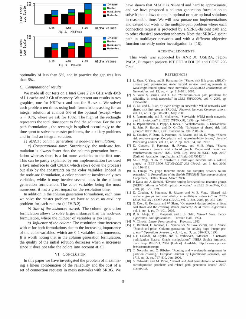
Fig. 2. NSFNET
Fig. 3. BRAZIL
optimality of less than 5%, and in practice the gap was lessthan 5‰.
C. Computational results
We made all our tests on aIntel Core 2 2.4 GHz with 4Mbof L1 cache and 2 Gb of memory. We present our results in twographics, one for NSFNET and one for BRAZIL . We solvedeach problem ten times using both formulations asking for aninteger solution at at most 5% of the optimal (except whenα = 0.75, where we ask for 10%). The high of the rectanglerepresents the total time spent to find the solution. For the arcpath formulation , the rectangle is splited accordingly to thetime spent to solve the master problems, the auxiliary problemsand to find an integral solution.
1) MACF: column generation vs node-arc formulation:a) Computational time:Surprisingly, the node-arc for-
mulation is always faster than the column generation formu-lation whereas there is a lot more variables in the first one.This can be partly explained by our implementation (we useda Java interface to call CPLEX which slows down the process)but also by the constraints on the color variables. Indeed inthe node-arc formulation, a color constraint involves onlytwovariables, while it may involve several ones in the columngeneration formulation. The color variables being the mostnumerous, it has a great impact on the resolution time.
In addition in the column generation formulation, each timewe solve the master problem, we have to solve an auxiliaryproblem for each request (cf IV-B.2).
b) Size of the instances solved:The column generationformulation allows to solve larger instances than the node-arcformulation, where the number of variables is too large.
c) Influence of the colors:The resolution time increaseswith α for both formulations due to the increasing importanceof the color variables, which are 0-1 variables and numerous.It is worth noting that in the column generation formulation,the quality of the initial solution decreases whenα increasessince it does not take the colors into account at all.
VI. CONCLUSION
In this paper we have investigated the problem of maximiz-ing a linear combination of the reliability and the cost of aset of connection requests in mesh networks with SRRG. We
have shown that MACF is NP-hard and hard to approximate,and we have proposed a column generation formulation tosolve it that allows to obtain optimal or near optimal solutionsin reasonable time. We will now pursue our implementationsand extend our work to the multiple-path problem where eachconnection request is protected by a SRRG-disjoint path andto other classical protection schemes. Note that SRRG-disjointpath in multilayer networks and with a different objectivefunction currently under investigation in [18].
ACKNOWLEDGMENTS
This work was supported by ANR JC OSERA, regionPACA, European projects IST FET AEOLUS and COST 293Graal.
REFERENCES
[1] L. Shen, X. Yang, and B. Ramamurthy, “Shared risk link group (SRLG)-diverse path provisioning under hybrid service level agreements inwavelength-routed optical mesh networks,”IEEE/ACM Transactions onNetworking, vol. 13, no. 4, pp. 918–931, 2005.
[2] S. Yuan, S. Varma, and J. Jue, “Minimum-color path problems forreliability in mesh networks,” inIEEE INFOCOM, vol. 4, 2005, pp.2658–2669.
[3] C. Liu and L. Ruan, “p-cycle design in survivable WDM networks withshared risk link groups (SRLGs),”Photonic Network Communications,vol. 11, no. 3, pp. 301–311, May 2006.
[4] S. Ramamurthy and B. Mukherjee, “Survivable WDM mesh networks,part 1: Protection,” inIEEE INFOCOM, 1999, pp. 744–751.
[5] D. Papadimitriou, F. Poppe, J. Jones, S. Venkatachalam,S. Dharanikota,R. Jain, R. Hartani, and D. Griffith, “Inference of shared risk linkgroups,” IETF Draft, OIF Contribution, OIF 2001-066.
[6] D. Coudert, P. Datta, S. Perennes, H. Rivano, and M.-E. Voge, “Sharedrisk resource group: Complexity and approximability issues,” ParallelProcessing Letters, vol. 17, no. 2, pp. 169–184, Jun. 2007.
[7] D. Coudert, S. Perennes, H. Rivano, and M.-E. Voge, “Sharedrisk resource groups and colored graph: Polynomial cases andtransformation issues,” HAL, Tech. Rep. inria-00175143, Sep. 2007.[Online]. Available: http://hal.inria.fr/inria-00175143/fr/
[8] M.-E. Voge, “How to transform a multilayer network into acoloredgraph,” in IEEE-LEOS ICTON/COST 293 GRAAL, vol. 3, Jun. 2006,pp. 116–119.
[9] A. Farago, “A graph theoretic model for complex networkfailurescenarios,” inProceedings of the Eighth INFORMS TelecommunicationsConference, Dallas, Texas, March 2006.
[10] P. Datta and A. Somani, “Diverse routing for shared riskresource groups(SRRG) failures in WDM optical networks,” inIEEE BroadNets, Oct.2004, pp. 120– 129.
[11] D. Coudert, S. Perennes, H. Rivano, and M.-E. Voge, “Shared riskresource groups and survivability in multilayer networks,” in IEEE-LEOS ICTON / COST 293 GRAAL, vol. 3, Jun. 2006, pp. 235–238.
[12] G. Even, G. Kortsarz, and W. Slany, “On network design problems: fixedcost flows and the covering steiner problem,”ACM Trans. Algorithms,vol. 1, no. 1, pp. 74–101, 2005.
[13] R. K. Ahuja, T. L. Magnanti, and J. B. Orlin,Network flows: theory,algorithms, and applications. Prentice Hall,, 1993.
[14] V. Chvatal,Linear Programming. Freeman, 1983.[15] C. Barnhart, E. Johnson, G. Nemhauser, M. Savelsbergh,and P. Vance,
“Branch-and-price: Column generation for solving huge integer pro-grams,”Operations Research, vol. 46, no. 3, pp. 316–329, 1998.
[16] J.-F. Lalande, M. Syska, and Y. Verhoeven, “Mascopt - a networkoptimization library: Graph manipulation,” INRIA Sophia Antipolis,Tech. Rep. RT-0293, 2004. [Online]. Available: http://www-sop.inria.fr/mascotte/mascopt
[17] T. Noronha and C. Ribeiro, “Routing and wavelength assignment bypartition coloring,” European Journal of Operational Research, vol.1713, no. 3, pp. 797–810, Jun. 2006.
[18] S. Orlowski and M. Pioro, “Primal and dual formulationsof networkreconfiguration problems and related path generation issues,” 2007,manuscript.
5

A New Framework for Efficient Shared SegmentProtection Scheme for WDM Networks
Brigitte Jaumard†, Florian Huc∗, Nazmum Bhuiyan‡, David Coudert∗∗ Mascotte project, I3S(CNRS/UNSA)/INRIA , Sophia-Antipolis, France
† GERAD, CIRRELT, and CIISE, Concordia University, Montreal, Canada‡ ECE, Concordia University, Montreal, Canada
Abstract— This work introduces a new shared segment protec-tion scheme that fully exploits the hop endpoints of the primarylogical hops (induced by the routing) without adding extra onesfor protection and ensure both node and link protection in anefficient manner both in terms of cost and bandwidth. Contraryto the link or path protection scheme, the segment protection onehas been less studied although it offers an interesting compromisebetween those two protection schemes, attempting to encompassall their advantages. We investigate two different Shared SegmentProtection (SSP) schemes: Basic Shared Segment Protection(BSSP) and Shared Segment Protection with segment Overlap(SSPO). The latter one is compared with the Short Leap SharedProtection (SLSP) scheme introduced by Ho and Mouftah (2002)in terms of architecture design and signaling mechanisms. Thekey difference lies in the overlapping of working segments inSLSP and of protection segments in SSPO. For both BSSP andSSPO schemes, we propose two novel efficient ILP formulations,based on a column generation mathematical modeling. While(SSPO) offers the advantage over (BSSP) to ensure both nodeand link protection, it is not necessarily more costly. Indeed,depending on the network topology and the traffic instances,it can be shown that none of the two SSP schemes dominatesthe other one. Therefore, the SSPO protection scheme shouldbe favored as it offers more protection, i.e., it adds the nodeprotection to the link protection.
I. I NTRODUCTION
Wavelength Division Multiplexing (WDM) is a well knowntechnology that allows an efficient use of the high bandwidthoffered by optical networks [1], [2]. Under WDM, laserbeams are used to implement fixed end-to-end connectionsin the network - called lightpaths - under the constraint thattwo lightpaths cannot share the same wavelength over thesame fiber. The Routing and Wavelength Assignment (RWA)problem consists thus in assigning a route in the network andawavelength to each lightpath. This NP-hard problem has beenwidely studied during the last 15 years (see, e.g., [3], [4])and optimal or near-optimal solutions can now be obtainedin reasonable time using proper integer linear programmingformulation ([5], [6]).
Since the bandwidth requirement of a request is usuallysmaller than the bandwidth offered by a single wavelength(Mbits versus Gbits), several requests may be groomed ona same wavelength in a Time Division Multiplexing (TDM)manner as it is the case in SONET/SDH networks. Theproblem of determining which requests to groom and whichroute to associate with the groomed requests corresponds tothe so-called Grooming, Routing and Wavelength Assignment
(GRWA) problem ([7], [8], [9], [10], [11]). To add a requestonto a wavelength, that is to groom it with other request,or to extract it from a wavelength, we use SONET Add-Drop Multiplexers (ADM) that convert optical signals intoelectronic ones and vice versa in order to conduct the add/dropoperations. Requests can be added or dropped from the trafficstream when they are in their electronic form. A segmentis a bundle of requests groomed together on a given wave-length λ between two nodes and that are not encounteringany electronic conversions, i.e., between two nodes that areequipped with aλ ADM. Therefore any working/protectionsegment uses two ports of ADMs devices, an output port atthe origin of the segment where the signal is converted fromelectronic to optical in order to add one or more requests, andan input port at the destination of the segment where the signalis converted from optical to electronic in order to drop one orseveral requests. ADMs consists in a set of blades, where eachblade is made of one output and one input port. The numberof blades used to route the traffic is a key factor in the overallcost of the network and its optimization is a problem in itself(see for example [12], [9]). We will use it as an estimation ofthe protection provisioning cost.
s dσw1 i1 σw2 i2 σw3
σp3σp2σp1
(a) BSSP
ds
σw2
σp
σw1
(b) shared protec-tion
Fig. 1. SSP Protection Scheme
In the current study, we focus onShared Segment Protectionschemes in the context of a sequential framework where theworking segments are first defined (using any given GRWAalgorithm) and then the protection scheme is defined. We

therefore assume that we are given a set of working paths,where each working path is either single-hop or multi-hop, i.e.,made of one or several (up to 3) working segments. Transportblades are installed at each endpoint of a working segment.This induces a natural segmentation of the lightpath that canbe used as a base for the protection scheme in order to saveon the network cost.
A first segment protection, called BSSP, is such that aprotection is defined for each working segment, and thereforesuch that both working and protection segments have thesame endpoints. A second segment protection, called SSPO,is such that for 3-hop working paths, we allow protectionsegments to encompass two working segments in order toreduce the bandwidth cost, but also and firstly to ensure nodeprotection. This entails some overlapping of the protectionsegments. In the next section, we will compare SSPO with theSLSP protection scheme of Mouftah and Ho [13] where theoverlapping is at the level of the working segments. In bothBSSP and SSPO, protection paths can be shared by severalnode and link disjoint working segments, it is illustrated inFigure I(b) whereσp protects two disjoint working segments.
The paper is organized as follows. In the next section, wehave a qualitative comparison of the BSSP, SSPO and SLSPprotection schemes. In the following sections, we investigateefficient Integer Linear Programming (ILP) formulations tosolve models for designing minimum cost protection schemesusing first the BSSP scheme (Section IV) and then the SSPOscheme (Section V). Both ILP formulations rely on columngeneration methods which have now been shown to be ex-tremely efficient for solving highly combinatorial problems,see, e.g., Barnhartet al. [14]. Conclusions are drawn in thelast section.
II. SHARED SEGMENT PROTECTION
BSSP protection has already been studied by Bouffard [15].Although less greedy in terms of bandwidth than shared linkprotection, and with a nice compromise for recovery timebetween link and path protection, it lacks a full protectionagainst node failures (i.e., failure of a device, as ADM, locatedat a node: in Figure I(a) neither nodei1 nor i2 are protected).
Ho and Mouftah introduced in [13] the Short Leap SharedProtection (SLSP) scheme as an extension of BSSP, simul-taneously protecting against node failure and fiber cut. InSLSP the working path is subdivided into several equal lengthand overlapped segments, each assigned (by the source node)a protection domain after the working path is selected. Inthis paper we consider a new protection scheme also pro-tecting against both fiber cut and node failure based on thesegmentation induced by the routing. TheShared SegmentProtection with Overlap(SSPO) scheme consists in protectingeach working segment simultaneously with at least an otherworking segment (except for a request routed on a singleworking segment, in this case the SSPO associate an endto end protection to the working segment). Since there areADMs at each endpoint of a working segment, it means thatat any node lying between two working segments, there is an
s d
s d
σp
σw1 i1 i2σw2 σw3
σp1 σp2
i1σw1 σw2 i2 σw3
(a) A request with 3 working segments
s σw1 i1 dσw2
σp
(b) A request with 2 working segments
s
σp
dσw
(c) A requestwith 1 workingsegments
Fig. 2. SSPO Protection Scheme
optical/electronic or electronic/optical conversion. Ifwe usethose nodes as endpoints for the protection segments, whetherthey are source or destination, we use only one input/outputof an ADM in order to put the protection segments in place.In the SSPO scheme, protection segments overlap as they aredesigned to protect several working segments simultaneouslyand not only a single working segment as in the SLSPscheme. This overlap between adjacent protection segmentsaims at ensuring node protection for all nodes, except for thesource and destination nodes. All different types of protectionsegments in the SSPO scheme, are shown on Figure 2. Notealso that a protection segment can be shared with severalworking segments as long as they are pairwise disjoint.
From BSSP and SSPO, several variants can be studied. Forexample if delay is not a main issue, the protection segmentmay be divided into several segments so that to increasesegment sharing and so to decrease the bandwidth needed forprotection.
Finally, note that shared risk group constraints can alsobe taken into account by modeling two working segmentsbelonging to the same risk group as conflicting workingsegments (see, e.g., [16]).
A. BSSP vs. SSPO
Depending on the network topology and the set of workingsegments (that depend in turn on the set of requests and theGRWA algorithm used to define these segments), there is nodominance of either the BSSP or the SSPO protection schemein terms of both bandwidth and cost as evaluated throughthe number of transport blades. Therefore, at equal or similarcost, SSPO should be favored over BSSP as it offers a better
2
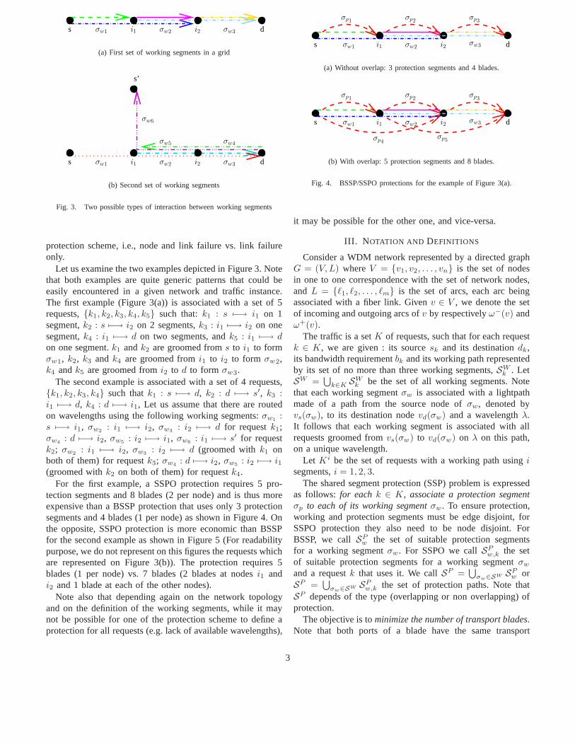
s di1 i2σw1 σw2 σw3
(a) First set of working segments in a grid
s dσw1 i1 σw2 i2 σw3
s’
σw6
σw5 σw4
(b) Second set of working segments
Fig. 3. Two possible types of interaction between working segments
protection scheme, i.e., node and link failure vs. link failureonly.
Let us examine the two examples depicted in Figure 3. Notethat both examples are quite generic patterns that could beeasily encountered in a given network and traffic instance.The first example (Figure 3(a)) is associated with a set of 5requests,k1, k2, k3, k4, k5 such that:k1 : s 7−→ i1 on 1segment,k2 : s 7−→ i2 on 2 segments,k3 : i1 7−→ i2 on onesegment,k4 : i1 7−→ d on two segments, andk5 : i1 7−→ don one segment.k1 andk2 are groomed froms to i1 to formσw1, k2, k3 andk4 are groomed fromi1 to i2 to form σw2,k4 andk5 are groomed fromi2 to d to form σw3.
The second example is associated with a set of 4 requests,k1, k2, k3, k4 such thatk1 : s 7−→ d, k2 : d 7−→ s′, k3 :i1 7−→ d, k4 : d 7−→ i1, Let us assume that there are routedon wavelengths using the following working segments:σw1
:s 7−→ i1, σw2
: i1 7−→ i2, σw3: i2 7−→ d for requestk1;
σw4: d 7−→ i2, σw5
: i2 7−→ i1, σw6: i1 7−→ s′ for request
k2; σw2: i1 7−→ i2, σw3
: i2 7−→ d (groomed withk1 onboth of them) for requestk3; σw4
: d 7−→ i2, σw5: i2 7−→ i1
(groomed withk2 on both of them) for requestk4.For the first example, a SSPO protection requires 5 pro-
tection segments and 8 blades (2 per node) and is thus moreexpensive than a BSSP protection that uses only 3 protectionsegments and 4 blades (1 per node) as shown in Figure 4. Onthe opposite, SSPO protection is more economic than BSSPfor the second example as shown in Figure 5 (For readabilitypurpose, we do not represent on this figures the requests whichare represented on Figure 3(b)). The protection requires 5blades (1 per node) vs. 7 blades (2 blades at nodesi1 andi2 and 1 blade at each of the other nodes).
Note also that depending again on the network topologyand on the definition of the working segments, while it maynot be possible for one of the protection scheme to define aprotection for all requests (e.g. lack of available wavelengths),
σp2 σp3σp1
s di1 i2 σw3σw2σw1
(a) Without overlap: 3 protection segments and 4 blades.
σp2 σp3σp1
σp4σp5
s di1 i2 σw3σw2σw1
(b) With overlap: 5 protection segments and 8 blades.
Fig. 4. BSSP/SSPO protections for the example of Figure 3(a).
it may be possible for the other one, and vice-versa.
III. N OTATION AND DEFINITIONS
Consider a WDM network represented by a directed graphG = (V, L) whereV = v1, v2, . . . , vn is the set of nodesin one to one correspondence with the set of network nodes,and L = ℓ1, ℓ2, . . . , ℓm is the set of arcs, each arc beingassociated with a fiber link. Givenv ∈ V , we denote the setof incoming and outgoing arcs ofv by respectivelyω−(v) andω+(v).
The traffic is a setK of requests, such that for each requestk ∈ K, we are given : its sourcesk and its destinationdk,its bandwidth requirementbk and its working path representedby its set of no more than three working segments,SW
k . LetSW =
⋃
k∈K SWk be the set of all working segments. Note
that each working segmentσw is associated with a lightpathmade of a path from the source node ofσw, denoted byvs(σw), to its destination nodevd(σw) and a wavelengthλ.It follows that each working segment is associated with allrequests groomed fromvs(σw) to vd(σw) on λ on this path,on a unique wavelength.
Let Ki be the set of requests with a working path usingisegments,i = 1, 2, 3.
The shared segment protection (SSP) problem is expressedas follows: for eachk ∈ K, associate a protection segmentσp to each of its working segmentσw. To ensure protection,working and protection segments must be edge disjoint, forSSPO protection they also need to be node disjoint. ForBSSP, we callSP
w the set of suitable protection segmentsfor a working segmentσw. For SSPO we callSP
w,k the setof suitable protection segments for a working segmentσw
and a requestk that uses it. We callSP =⋃
σw∈SW SPw or
SP =⋃
σw∈SW SPw,k the set of protection paths. Note that
SP depends of the type (overlapping or non overlapping) ofprotection.
The objective is tominimize the number of transport blades.Note that both ports of a blade have the same transport
3

σp4σp5
s di1 i2
σp3σp2σp1
s’
σp6
(a) Without overlap: 6 protection segments and 7 blades.
s di1 i2
s’
σp4
σp1 σp3
σp2
(b) With overlap: 4 protection segments and 5 blades.
Fig. 5. BSSP/SSPO protections for the example Figure 3(b).
capacity, but not necessarily the same wavelength. Moreover,a transport blade cannot be such that one of its port is usedin a working path, and the other one in a protection path.
Two protection segments are in conflict if they use the samewavelength on the same fiber link since we can not use themsimultaneously. Two working segments can be protected bytwo conflicting protection segments if and only if they do notshare any fiber link. For SSPO protection, we add the conditionthat they do not share any node except for their endpoints.Indeed, if a fiber link shared by two working segments is cut,we need to reroute each pair of working segments on twodifferent alternative paths. We use the following parameter:
δww′ =
1 if σw andσw′ can be protected by the same
protection segment
0 otherwise.
IV. BSSP PROTECTION SCHEME
In this section, we will restrict our attention to the BSSPprotection. We propose to investigate a column generationformulation in order to find optimal protection design withthe BSSP scheme. We will outline the main features andadvantages of column generation formulations in the nextparagraph, and then detail the proposed model in the followingparagraphs.
A. An Overview on Column Generation Models
Column generation techniques offer solution methods forlinear programs with a very large number of variables (e.g.,exponential) where constraints can be expressed implicitly.They rely on a decomposition of the initial linear programinto themaster problemand thepricing problem. The masterproblem corresponds to a linear program associated with arestricted constraint matrix, with respect to the number ofvariables (or columns) of the initial constraint matrix. Thepricing problem is defined by the optimization of the so-calledreduced cost subject to the implicit constraints expressedbythe coefficients of the constraint matrix of the master problem.In some cases, there may be several pricing problems if, e.g.,there are several types of columns.
The column generation solution scheme is similar to thatof the simplex algorithm: it is an iterative process where, ateach step, we attempt to add one or more columns to theconstraint matrix of the master problem in order to improve thevalue of its objective function. The search for such columnsis made through the solution of the pricing problem. If itsoutcome corresponds to one or more columns with a negativereduced cost (assuming we deal with minimization), then itentails an improvement of the value of the master objectivefunction; otherwise, if no solution of the pricing problem canbe identified with a negative cost, we then conclude that thecurrent solution is indeed optimal.
Column generation can be combined with branch-and-bound techniques for solving integer linear programs witha large number of variables, see [14] for a nice overview.Branching rules have to be devised properly in order to avoidgenerating a huge number of subproblems in the search treeassociated with the branch-and-bound, either by branchingon the variables of the master problem using cuts, or bybranching on the variables of the pricing problem usingclassical branching schemes or cuts.
B. The CG-BSSP Column Generation Model with WavelengthBSSP Protection Configurations
We propose a column generation model, denoted by CG-BSSP, based onwavelength BSSP protection configurations.For each wavelengthλ, we define awavelength BSSP protec-tion configuration, as a set of protection segments followingthe BSSP protection scheme, all routed onλ, which protecta given set of working segments that are not necessarilyrouted on the wavelengthλ. In order to reduce the number ofconfigurations to be explored, we only consider the maximalones, i.e., those are not embedded in larger ones with identicalcost.
Such a column generation model leads to a decompositionwhere the master problem takes care of selecting the bestconfigurations, one for each wavelength, i.e., the set of config-urations that minimizes the cost as evaluated by the numberof transport blades. The pricing problem identifies the bestpossible configurations, and therefore handles the constraintsassociated with the definition of a protection segment, i.e., nolink sharing between a working segment and its protection,
4
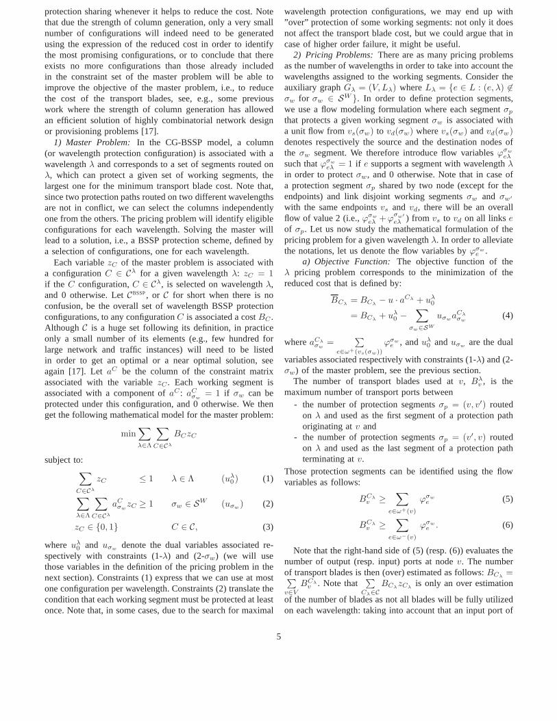
protection sharing whenever it helps to reduce the cost. Notethat due the strength of column generation, only a very smallnumber of configurations will indeed need to be generatedusing the expression of the reduced cost in order to identifythe most promising configurations, or to conclude that thereexists no more configurations than those already includedin the constraint set of the master problem will be able toimprove the objective of the master problem, i.e., to reducethe cost of the transport blades, see, e.g., some previouswork where the strength of column generation has allowedan efficient solution of highly combinatorial network designor provisioning problems [17].
1) Master Problem: In the CG-BSSP model, a column(or wavelength protection configuration) is associated with awavelengthλ and corresponds to a set of segments routed onλ, which can protect a given set of working segments, thelargest one for the minimum transport blade cost. Note that,since two protection paths routed on two different wavelengthsare not in conflict, we can select the columns independentlyone from the others. The pricing problem will identify eligibleconfigurations for each wavelength. Solving the master willlead to a solution, i.e., a BSSP protection scheme, defined bya selection of configurations, one for each wavelength.
Each variablezC of the master problem is associated witha configurationC ∈ Cλ for a given wavelengthλ: zC = 1if the C configuration,C ∈ Cλ, is selected on wavelengthλ,and 0 otherwise. LetCBSSP, or C for short when there is noconfusion, be the overall set of wavelength BSSP protectionconfigurations, to any configurationC is associated a costBC .Although C is a huge set following its definition, in practiceonly a small number of its elements (e.g., few hundred forlarge network and traffic instances) will need to be listedin order to get an optimal or a near optimal solution, seeagain [17]. LetaC be the column of the constraint matrixassociated with the variablezC . Each working segment isassociated with a component ofaC : aC
σw= 1 if σw can be
protected under this configuration, and 0 otherwise. We thenget the following mathematical model for the master problem:
min∑
λ∈Λ
∑
C∈Cλ
BCzC
subject to:∑
C∈Cλ
zC ≤ 1 λ ∈ Λ (uλ0 ) (1)
∑
λ∈Λ
∑
C∈Cλ
aCσw
zC ≥ 1 σw ∈ SW (uσw) (2)
zC ∈ 0, 1 C ∈ C, (3)
where uλ0 and uσw
denote the dual variables associated re-spectively with constraints (1-λ) and (2-σw) (we will usethose variables in the definition of the pricing problem in thenext section). Constraints (1) express that we can use at mostone configuration per wavelength. Constraints (2) translate thecondition that each working segment must be protected at leastonce. Note that, in some cases, due to the search for maximal
wavelength protection configurations, we may end up with”over” protection of some working segments: not only it doesnot affect the transport blade cost, but we could argue that incase of higher order failure, it might be useful.
2) Pricing Problems:There are as many pricing problemsas the number of wavelengths in order to take into account thewavelengths assigned to the working segments. Consider theauxiliary graphGλ = (V, Lλ) whereLλ = e ∈ L : (e, λ) 6∈σw for σw ∈ SW . In order to define protection segments,we use a flow modeling formulation where each segmentσp
that protects a given working segmentσw is associated witha unit flow fromvs(σw) to vd(σw) wherevs(σw) andvd(σw)denotes respectively the source and the destination nodes ofthe σw segment. We therefore introduce flow variablesϕσw
eλ
such thatϕσw
eλ = 1 if e supports a segment with wavelengthλin order to protectσw, and 0 otherwise. Note that in case ofa protection segmentσp shared by two node (except for theendpoints) and link disjoint working segmentsσw and σw′
with the same endpointsvs and vd, there will be an overallflow of value 2 (i.e.,ϕσw
eλ +ϕσ
w′
eλ ) from vs to vd on all linkseof σp. Let us now study the mathematical formulation of thepricing problem for a given wavelengthλ. In order to alleviatethe notations, let us denote the flow variables byϕσw
e .a) Objective Function: The objective function of the
λ pricing problem corresponds to the minimization of thereduced cost that is defined by:
BCλ= BCλ
− u · aCλ + uλ0
= BCλ+ uλ
0 −∑
σw∈SW
uσwaCλ
σw(4)
whereaCλ
σw=
∑
e∈ω+(vs(σw))
ϕσw
e , anduλ0 anduσw
are the dual
variables associated respectively with constraints (1-λ) and (2-σw) of the master problem, see the previous section.
The number of transport blades used atv, Bλv , is the
maximum number of transport ports between- the number of protection segmentsσp = (v, v′) routed
on λ and used as the first segment of a protection pathoriginating atv and
- the number of protection segmentsσp = (v′, v) routedon λ and used as the last segment of a protection pathterminating atv.
Those protection segments can be identified using the flowvariables as follows:
BCλ
v ≥∑
e∈ω+(v)
ϕσw
e (5)
BCλ
v ≥∑
e∈ω−(v)
ϕσw
e . (6)
Note that the right-hand side of (5) (resp. (6)) evaluates thenumber of output (resp. input) ports at nodev. The numberof transport blades is then (over) estimated as follows:BCλ
=∑
v∈V
BCλ
v . Note that∑
Cλ∈C
BCλzCλ
is only an over estimation
of the number of blades as not all blades will be fully utilizedon each wavelength: taking into account that an input port of
5
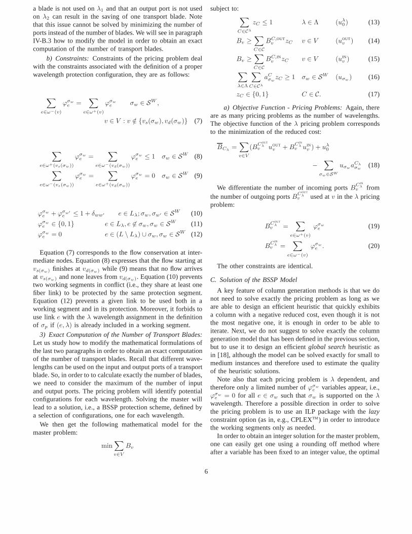
a blade is not used onλ1 and that an output port is not usedon λ2 can result in the saving of one transport blade. Notethat this issue cannot be solved by minimizing the number ofports instead of the number of blades. We will see in paragraphIV-B.3 how to modify the model in order to obtain an exactcomputation of the number of transport blades.
b) Constraints: Constraints of the pricing problem dealwith the constraints associated with the definition of a properwavelength protection configuration, they are as follows:
∑
e∈ω−(v)
ϕσw
e =∑
e∈ω+(v)
ϕσw
e σw ∈ SW ,
v ∈ V : v /∈ vs(σw), vd(σw) (7)
∑
e∈ω+(vs(σw))
ϕσw
e =∑
e∈ω−(vd(σw))
ϕσw
e ≤ 1 σw ∈ SW (8)
∑
e∈ω−(vs(σw))
ϕσw
e =∑
e∈ω+(vd(σw))
ϕσw
e = 0 σw ∈ SW (9)
ϕσw
e + ϕσw′
e ≤ 1 + δww′ e ∈ Lλ; σw, σw′ ∈ SW (10)
ϕσw
e ∈ 0, 1 e ∈ Lλ, e 6∈ σw, σw ∈ SW (11)
ϕσw
e = 0 e ∈ (L \ Lλ) ∪ σw, σw ∈ SW (12)
Equation (7) corresponds to the flow conservation at inter-mediate nodes. Equation (8) expresses that the flow startingatvs(σw) finishes atvd(σw) while (9) means that no flow arrivesat vs(σw) and none leaves fromvd(σw). Equation (10) preventstwo working segments in conflict (i.e., they share at least onefiber link) to be protected by the same protection segment.Equation (12) prevents a given link to be used both in aworking segment and in its protection. Moreover, it forbidstouse linke with the λ wavelength assignment in the definitionof σp if (e, λ) is already included in a working segment.
3) Exact Computation of the Number of Transport Blades:Let us study how to modify the mathematical formulations ofthe last two paragraphs in order to obtain an exact computationof the number of transport blades. Recall that different wave-lengths can be used on the input and output ports of a transportblade. So, in order to to calculate exactly the number of blades,we need to consider the maximum of the number of inputand output ports. The pricing problem will identify potentialconfigurations for each wavelength. Solving the master willlead to a solution, i.e., a BSSP protection scheme, defined bya selection of configurations, one for each wavelength.
We then get the following mathematical model for themaster problem:
min∑
v∈V
Bv
subject to:∑
C∈Cλ
zC ≤ 1 λ ∈ Λ (uλ0 ) (13)
Bv ≥∑
C∈C
BC,OUTv zC v ∈ V (uOUT
v ) (14)
Bv ≥∑
C∈C
BC,INv zC v ∈ V (uIN
v ) (15)
∑
λ∈Λ
∑
C∈Cλ
aCσw
zC ≥ 1 σw ∈ SW (uσw) (16)
zC ∈ 0, 1 C ∈ C. (17)
a) Objective Function - Pricing Problems:Again, thereare as many pricing problems as the number of wavelengths.The objective function of theλ pricing problem correspondsto the minimization of the reduced cost:
BCλ=
∑
v∈V
(BCOUT
λ
v uOUTv + B
C INλ
v uINv ) + uλ
0
−∑
σw∈SW
uσwaCλ
σw(18)
We differentiate the number of incoming portsBC IN
λ
v fromthe number of outgoing portsBCOUT
λ
v used atv in theλ pricingproblem:
BCOUT
λ
v =∑
e∈ω+(v)
ϕσw
e (19)
BC IN
λ
v =∑
e∈ω−(v)
ϕσw
e . (20)
The other constraints are identical.
C. Solution of the BSSP Model
A key feature of column generation methods is that we donot need to solve exactly the pricing problem as long as weare able to design an efficient heuristic that quickly exhibitsa column with a negative reduced cost, even though it is notthe most negative one, it is enough in order to be able toiterate. Next, we do not suggest to solve exactly the columngeneration model that has been defined in the previous section,but to use it to design an efficientglobal searchheuristic asin [18], although the model can be solved exactly for small tomedium instances and therefore used to estimate the qualityof the heuristic solutions.
Note also that each pricing problem isλ dependent, andtherefore only a limited number ofϕσw
e variables appear, i.e.,ϕσw
e = 0 for all e ∈ σw such thatσw is supported on theλwavelength. Therefore a possible direction in order to solvethe pricing problem is to use an ILP package with thelazyconstraint option (as in, e.g., CPLEXTM ) in order to introducethe working segments only as needed.
In order to obtain an integer solution for the master problem,one can easily get one using a rounding off method whereafter a variable has been fixed to an integer value, the optimal
6
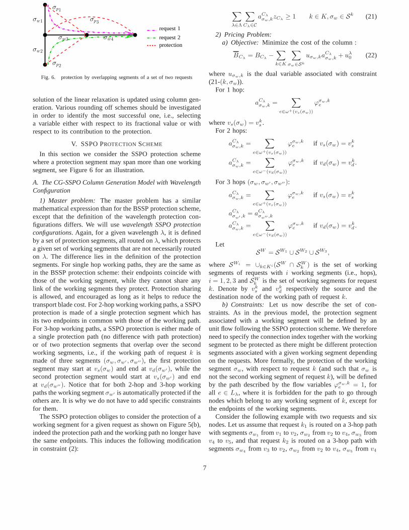
request 1
request 2protection
σw2
σw1
σw4σw3
σp3
σp1
σp2
Fig. 6. protection by overlapping segments of a set of two requests
solution of the linear relaxation is updated using column gen-eration. Various rounding off schemes should be investigatedin order to identify the most successful one, i.e., selectinga variable either with respect to its fractional value or withrespect to its contribution to the protection.
V. SSPO PROTECTION SCHEME
In this section we consider the SSPO protection schemewhere a protection segment may span more than one workingsegment, see Figure 6 for an illustration.
A. The CG-SSPO Column Generation Model with WavelengthConfiguration
1) Master problem: The master problem has a similarmathematical expression than for the BSSP protection scheme,except that the definition of the wavelength protection con-figurations differs. We will usewavelength SSPO protectionconfigurations. Again, for a given wavelengthλ, it is definedby a set of protection segments, all routed onλ, which protectsa given set of working segments that are not necessarily routedon λ. The difference lies in the definition of the protectionsegments. For single hop working paths, they are the same asin the BSSP protection scheme: their endpoints coincide withthose of the working segment, while they cannot share anylink of the working segments they protect. Protection sharingis allowed, and encouraged as long as it helps to reduce thetransport blade cost. For 2-hop working working paths, a SSPOprotection is made of a single protection segment which hasits two endpoints in common with those of the working path.For 3-hop working paths, a SSPO protection is either made ofa single protection path (no difference with path protection)or of two protection segments that overlap over the secondworking segments, i.e., if the working path of requestk ismade of three segments(σw, σw′ , σw′′), the first protectionsegment may start atvs(σw) and end atvd(σw′), while thesecond protection segment would start atvs(σw′) and endat vd(σw′′). Notice that for both 2-hop and 3-hop workingpaths the working segmentσw′ is automatically protected if theothers are. It is why we do not have to add specific constraintsfor them.
The SSPO protection obliges to consider the protection of aworking segment for a given request as shown on Figure 5(b),indeed the protection path and the working path no longer havethe same endpoints. This induces the following modificationin constraint (2):
∑
λ∈Λ
∑
Cλ∈C
aCλ
σw,kzCλ≥ 1 k ∈ K, σw ∈ Sk (21)
2) Pricing Problem:a) Objective: Minimize the cost of the column :
BCλ= BCλ
−∑
k∈K
∑
σw∈Sk
uσw,kaCλ
σw,k + uλ0 (22)
where uσw,k is the dual variable associated with constraint(21-(k, σw)).
For 1 hop:
aCλ
σw,k =∑
e∈ω+(vs(σw))
ϕσw ,ke
wherevs(σw) = vks .
For 2 hops:
aCλ
σw,k =∑
e∈ω+(vs(σw))
ϕσw ,ke if vs(σw) = vk
s
aCλ
σw,k =∑
e∈ω−(vd(σw))
ϕσw ,ke if vd(σw) = vk
d .
For 3 hops(σw , σw′ , σw′′):
aCλ
σw,k =∑
e∈ω+(vs(σw))
ϕσw ,ke if vs(σw) = vk
s
aCλ
σw′ ,k
= aCλ
σw′′ ,k
aCλ
σw,k =∑
e∈ω−(vd(σw))
ϕσw ,ke if vd(σw) = vk
d .
LetSW = SW1 ∪ SW2 ∪ SW3 ,
where SWi = ∪k∈Ki(SW ∩ SWk ) is the set of working
segments of requests withi working segments (i.e., hops),i = 1, 2, 3 andSW
k is the set of working segments for requestk. Denote byvk
s and vkd respectively the source and the
destination node of the working path of requestk.b) Constraints: Let us now describe the set of con-
straints. As in the previous model, the protection segmentassociated with a working segment will be defined by anunit flow following the SSPO protection scheme. We thereforeneed to specify the connection index together with the workingsegment to be protected as there might be different protectionsegments associated with a given working segment dependingon the requests. More formally, the protection of the workingsegmentσw, with respect to requestk (and such thatσw isnot the second working segment of requestk), will be definedby the path described by the flow variablesϕσw ,k
e = 1, forall e ∈ Lλ, where it is forbidden for the path to go throughnodes which belong to any working segment ofk, except forthe endpoints of the working segments.
Consider the following example with two requests and sixnodes. Let us assume that requestk1 is routed on a 3-hop pathwith segmentsσw1
from v1 to v2, σw2from v2 to v4, σw3
fromv4 to v5, and that requestk2 is routed on a 3-hop path withsegmentsσw4
from v3 to v2, σw2from v2 to v4, σw5
from v4
7

to v6. Following the SSPO scheme, we need four protectionsegments:σp1
from v1 to v4 andσp2from v2 to v5 to ensure
protection fork1; σp3from v3 to v4 andσp4
from v2 to v6 toensure protection fork2. We therefore have two flows goingout ofv2, one for each request, both ensuring the protection ofthe segmentσw2
and the protection of an additional segment.Same remark for the incoming flows atv4.
∑
e∈ω−(v)
ϕσw,ke =
∑
e∈ω+(v)
ϕσw ,ke
v ∈ V \⋃
σ∈SW
k
σ, σw ∈ SWk , k ∈ K (23)
∑
e∈ω−(v)
ϕσw,ke =
∑
e∈ω+(v)
ϕσw ,ke = 0
v ∈⋃
σ∈SW
k
σ : v /∈⋃
σ∈SW
k
vs(σ), vd(σ),
σw ∈ SWk , k ∈ K (24)
∑
e∈ω+(vs(σw))
ϕσw ,ke =
∑
e∈ω−(vd(σw))
ϕσw ,ke ≤ 1 σw ∈ K1 (25)
∑
e∈ω+(vs(σw))
ϕσw,ke =
∑
e∈ω−(vd(σw′ ))
ϕσw ,ke ≤ 1 (26)
∑
e∈ω−(vd(σw))
ϕσw ,ke =
∑
e∈ω+(vs(σw′ ))
ϕσw ,ke = 0 (27)
vs(σw) = vks ,
σw, σw′ = SWk , k ∈ K2 (28)
For 3-hop working paths, constraints (29) express that theprotection segment starts atvs(σw) and ends at eithervd(σw′)or vd(σw′′), whereσw′ is the second working segment andσw′′ the third.
∑
e∈ω+(vs(σw))
ϕσw ,ke =
∑
e∈ω−(vd(σw′ ))
ϕσw ,ke
+∑
e∈ω−(vd(σw′′ ))
ϕσw ,ke ≤ 1
vs(σw) = vks , vd(σw′′ ) = vk
d
(σw , σw′ , σw′′) = SWk , k ∈ K3 (29)
Constraints (30) applies for the third working segmentσw′′ ,expressing that the protection segment starts at eithervs(σw)or vs(σw′) and ends atvd(σw′′ ).
∑
e∈ω+(vs(σw))
ϕσw ,ke +
∑
e∈ω+(vs(σw′ ))
ϕσw ,ke
=∑
e∈ω−(vd(σw′′ ))
ϕσw ,ke ≤ 1
vs(σw) = vks , vd(σw′′ ) = vk
d
(σw , σw′ , σw′′) = SWk , k ∈ K3 (30)
We do not need constraints for defining a protection for thesecond working segment of a 3-hop request, as it is protectedby the same protection segment than the first or the lastworking segment.
Constraints (31) prevent from an useless use of intermediatenodes.
∑
e∈ω−(vs(σw)
ϕσw ,ke =
∑
e∈ω+(vd(σw′ ))
ϕσw ,ke = 0
vs(σw) = vks , vd(σw′′) = vk
d
(σw, σw′ , σw′′) = SWk , k ∈ K3 (31)
∑
e∈ω−(vks)
ϕσw ,ke = 0 σw ∈ SW
k , k ∈ K (32)
∑
e∈ω+(vk
d)
ϕσw ,ke = 0 σw ∈ SW
k , k ∈ K (33)
ϕσw ,ke + ϕσ
w′ ,k′
e ≤ 1 + δww′ e ∈ Lλ; σw, σw′ ∈ SW ,
k, k′ ∈ K (10’)
ϕσw ,ke ∈ 0, 1 e ∈ Lλ \ (
⋃
σw∈SW
k
σw), σw ∈ SW ,
k ∈ K (11’)
ϕσw ,ke = 0 e ∈ (L \ Lλ)
⋃
σw∈SW
k
σw, σw ∈ SW ,
k ∈ K (12’)
Constraints (23) correspond to the classical flow conserva-tion constraints.
For single-hop working paths, constraints are the same thanin the CG-BSSP model, i.e, corresponds to constraints (23) -(25), (32) - (33), (10’), (11’) and (12’) with the addition ofconstraints (24) in order to prevent the protection path to usea node of the working path.
For 2-hop working paths, the only possibility for a protec-tion segment is to go from the source to the destination of therequest, without going any node or link already involved in oneof the working segments of the working path. Constraints (26)apply for the first working segmentσw, expressing that theprotection segment starts atvs(σw) and ends atvd(σw′), whereσw′ is the second working segment. Equation (27) forbid theuse of the end node of the first working segment, to ensure itsprotection. We do not need constraints for the second workingsegment of a 2-hop request, as its is protected by the sameprotection segment than the first working segment.
Constraints (10’), (11’) and (12 bid) are similar than in thepricing problem of the CG-BSSP column generation model,except thatσw take value in allSW
k .
B. Solution of the SSPO Model
We can use the same techniques than those proposed forthe BSSP model.
8

VI. CONCLUSION
In this paper we investigated a new segment protectionscheme in WDM networks in the context of traffic grooming.The cost of the protection is measured through the overallnumber of ADMs required for the protection segments. Weinvestigated two protection schemes assuming a sequentialapproach, where we define the protection framework once theworking paths, made of a set of 1 to 3 working segments,has been defined using a given GRWA algorithm. The firstprotection scheme, called (BSSP), is such that each workingsegment is protected individually, while in the second one,called (SSPO), each working segment is protected simulta-neously with others. Advantages of the SSPO scheme lie inthat it protects the network against both node failure and fibercut. We showed, using generic examples that none of thetwo protection technique dominates the other and we gave forboth of them an ILP formulation using column generation. Weare currently working on the implementation of these modelstechniques and performance results will be reported soon tobetter assess the efficiency of the SSPO scheme. Therefore, asequal or similar cost, the SSPO protection framework shouldbe favored as it offers a better protection, i.e., offers protectionagainst both node and link failure.
ACKNOWLEDGMENT
Work of B. Jaumard has been supported by a ConcordiaResearch Chair on the Optimization of Communication Net-works and by a NSERC grant. Work of F. Huc and D. Couderthas been partially supported by ANR-JC OSERA, INRIA,European project IST FET AEOLUS, COST 293 and RegionProvence Alpes Cote d’Azur PACA.
REFERENCES
[1] B. Mukherjee,Optical WDM Networks. Springer, 2006.[2] R. Ramaswami and K. Sivarajan,Optical Networks - A Practical
Perspective, 2nd ed. Morgan Kaufmann, 2002.[3] R. Dutta and G. Rouskas, “A survey of virtual topology design al-
gorithms for wavelength routed optical networks,”Optical NetworksMagazine, vol. 1, no. 1, pp. 73–89, January 2000.
[4] H. Zang, J. P. Jue, and B. Mukherjee, “A review of routing andwavelength assignment approaches for wavelength-routed optical WDMnetworks,”Optical Networks Magazine, pp. 47–60, January 2000.
[5] B. Jaumard, C. Meyer, and B. Thiongane, “Decomposition methods forthe RWA problem,” submitted for Publication.
[6] ——, “ILP formulations for the RWA problem for symmetrical systems,”in Handbook for Optimization in Telecommunications, P. Pardalos andM. Resende, Eds. Kluwer, 2006, ch. 23, pp. 637–678.
[7] R. Dutta and G. Rouskas, “Traffic grooming in WDM networks: Past andfuture,” IEEE Network, vol. 16, no. 6, pp. 46–56, November/December2002.
[8] E. Modiano and P. Lin, “Traffic grooming in WDM networks,”IEEECommunications Magazine, vol. 39, no. 7, pp. 124–129, Jul. 2001.
[9] A. Somani, Survivability and Traffic Grooming in WDM Optical Net-works. Cambridge Univwersity Press, Jan. 2006.
[10] K. Zhu and B. Mukherjee, “A review of traffic grooming in WDM opticalnetworks: Architectures and challenges,”Optical Networks Magazine,vol. 4, no. 2, pp. 55–64, March/April 2003.
[11] J. Hu and B. Leida, “Traffic grooming, routing, and wavelength assign-ment in optical WDM mesh networks,” inIEEE InfoCom, 2004.
[12] S. Huang, R. Dutta, and G. N. Rouskas, “Traffic grooming in path, star,and tree networks: Complexity, bounds, and algorithms,”IEEE Journalon Selected Areas in Communications, 2006.
[13] P.-H. Ho and H. T. Mouftah, “A framework for service-guaranteed sharedprotection in wdm mesh networks,”IEEE Communications Magazine,pp. 97–103, February 2002.
[14] C. Barnhart, E. Johnson, G. Nemhauser, M. Savelsbergh,and P. Vance,“Branch-and-price: Column generation for solving huge integer pro-grams,” Operations Research, vol. 46, no. 3, pp. 316–329, May-June1998.
[15] A. Bouffard, “Dimensionnement GRWA et protection par segment dansles rA c©seaux optiques WDM,” Master’s thesis, Universite de Montreal,Canada, 2005.
[16] L. Shen, X. Yang, and B. Ramamurthy, “Shared risk link group (srlg)-diverse path provisioning under hybrid service level agreements inwavelength-routed optical mesh networks,”IEEE/ACM Transactions onNetworking, vol 13, pp. 918, August 2005.
[17] T. Hemazro, B. Jaumard, and O. Marcotte, “A column generationand branch-and-cut algorithm for the channel assignment problem,” toappear in Computers and Operations Research, 2007.
[18] B. Jaumard, B. Vignac, and F. Vanderbeck, “An efficient global searchheuristic for the grwa proble,”submitted for publication, 2007.
9

274 Annexes

Annexe E
Reroutage de connexions etPathwidth
E.1 A distributed algorithm for computing and updatingthe process number of a forest
Rapport de recherche, présenté à ALGOTEL08 puis à DISC08 en version étendue.
E.2 Pathwidth of Outerplanar Graphs
Article publié dans JGT.
E.3 On the Pathwidth of Planar Graphs
Article accepté pour publication dans Journal of Discrete Maths.
275

appor t de r ech er ch e
ISS
N02
49-6
399
ISR
NIN
RIA
/RR
--65
60--
FR
+E
NG
Thème COM
INSTITUT NATIONAL DE RECHERCHE EN INFORMATIQUE ET EN AUTOMATIQUE
A distributed algorithm for computing and updatingthe process number of a forest
David Coudert — Florian Huc — Dorian Mazauric
N° 6560
June 2008
inria
-002
8830
4, v
ersi
on 3
- 27
Jun
200
8

inria
-002
8830
4, v
ersi
on 3
- 27
Jun
200
8

Unité de recherche INRIA Sophia Antipolis2004, route des Lucioles, BP 93, 06902 Sophia Antipolis Cedex (France)
Téléphone : +33 4 92 38 77 77 — Télécopie : +33 4 92 38 77 65
A distributed algorithm for computing and updating the proc essnumber of a forest
David Coudert∗ , Florian Huc∗ , Dorian Mazauric∗
Thème COM — Systèmes communicantsProjet MASCOTTE
Rapport de recherche n° 6560 — June 2008 — 16 pages
Abstract: In this paper, we present a distributed algorithm to computevarious parameters of a treesuch as the process number, the edge search number or the nodesearch number and so the path-width. This algorithm requiresn steps, an overall computation time ofO(nlogn), andn messages ofsize log3n+3. We then propose a distributed algorithm to update the process number (or the nodesearch number, or the edge search number) of each component of a forest after adding or deletingan edge. This second algorithm requiresO(D) steps, an overall computation time ofO(D logn), andO(D) messages of size log3 n+ 3, whereD is the diameter of the modified connected component.Finally, we show how to extend our algorithms to trees and forests of unknown size using messagesof less than 2α+4+ ε bits, whereα is the parameter to be determined andε = 1 for updates algo-rithms.
Key-words: pathwidth, process number, search number, distributed algorithm.
MASCOTTE, INRIA, I3S(CNRS/UNSA), Sophia Antipolis, [email protected]
∗ This work was partially funded by the European projectsIST FET AEOLUSand COST 293 GRAAL , and done within theCRC CORSOwith France Telecom R&D.
inria
-002
8830
4, v
ersi
on 3
- 27
Jun
200
8

Un algorithme distribué pour le calcul et la mise à jour duprocess number d’une forêt
Résumé : Dans cet article, nous présentons un algorithme distribué permettant de calculer diversparamètres d’un arbre tel le process number, la pathwidth etl’edge search number. Cet algorithmenécessiten étapes, a un temps d’exécution deO(nlogn) et génèren messages de taille log3 n+ 3.Nous montrons ensuite comment il peut servir a mettre à jour le process number (ou la pathwidth oul’edge search number) de chaque composante d’un forêt aprèsl’ajout ou la suppression d’une arête.En fin on montre que cela peut être fait même si la taille de la forêt est inconnue.
Mots-clés : pathwidth, process number, search number, algorithme distribué
inria
-002
8830
4, v
ersi
on 3
- 27
Jun
200
8

A distributed algorithm for the process number of a forest 3
1 Introduction
Treewidth and pathwidth have been introduced by Robertson and Seymour [11] as part of the graphminor project. By definition, the treewidth of a tree is one, but its pathwidth might be up to logn. Alinear time centralized algorithms to compute the pathwidth of a tree has been proposed in [5, 12, 13],but so far no dynamic algorithm exists.
The algorithmic counter part of the notion of pathwidth is the node searching problem [8]. Itconsists in finding an invisible and fast fugitive in a graph using the smallest set of agents. Theminimun number of agents needed gives the pathwidth. Other graph invariants closely related tothe notion of pathwidth have been proposed such as the process number [2, 3] and the edge searchnumber [9]. For this two invariants it is not known if they arestrictly equivalent to the pathwidth ornot.
In this paper, we propose a dynamic algorithm to compute those different parameters on trees andto update them in a forest after the addition or deletion of anedge. We also show that no distributedalgorithm can always transmit a number of bits linear inn and give a characterisation of the treeswhose process number and edge search number equals their pathwidth. To present our results, weconcentrate on the process number.
As mentioned before the process number of a (di)graph has been introduced to model a routingreconfiguration problem in WDM or WiFi networks in [2, 3]. Thegraph represents a set of tasks thathave to be realized. Aprocess strategyis a serie of actions in order to realize all the tasks representedby the graph. It finishes when all the nodes of the graph areprocessed. In order to process the graph,the three actions we can do are:
(1) put an agent on a node.
(2) remove an agent from a node if all its neighbors are eitherprocessed or occupied by an agent.The node is now processed.
(3) process a node if all its neighbors are occupied by an agent (the node is surrounded).
A p-process strategyis a strategy which process the graph usingp agents. Theprocess numberofa graphG, pn(G), is the smallestp such that ap-process strategy exists. For example, a star hasprocess number 1 (we place an agent on its center), a path of length at least 4 has process number 2, acycle of size 5 or more has process number 3, and an×n grid has process numbern+1. Moreover,it has been proved in [2, 3] that pw(G) ≤ pn(G) ≤ pw(G) + 1, where pw(G) is thepathwidthofG [11].
The node search number [8], ns(G), can be defined similarly except that we only use rules (1)and (2). It was proved by Elliset al.[5] that ns(G) = pw(G)+1, and by Kinnersley [7] that pw(G) =vs(G), where vs(G) is thevertex separationof G. Those results show that the vertex separation, thenode search number and the pathwidth are equivalent. Pleaserefer to recent surveys [6, 4] for moreinformation.
The following Theorem gives a construction which enforces each parameter to grow by 1, whichimplies that for any tree ns(T), es(T), pw(T), vs(T), and pn(T) are less than log3(n).
RR n° 6560
inria
-002
8830
4, v
ersi
on 3
- 27
Jun
200
8
4 Coudert, Huc, Mazauric
Theorem 1 ([2] and [10]) Let G1,G2 and G3 be three connected graphs such thatvs(Gi) = vs,ns(Gi) = ns andpn(Gi) = p, 1 ≤ i ≤ 3. We construct the graph G by putting one copy of each ofthe Gi , and we add one node v that has exactly one neighbour in each ofthe Gi , 1≤ i ≤ 3. Thenvs(G) = vs+1, ns(G) = ns+1 andpn(G) = p+1.
The algorithm we propose is based on the decomposition of a tree into subtrees forming ahier-archical decomposition. It is fully distributed, can be executed in an asynchronousenvironment andthe construction of the hierarchical decomposition requires only a small amount of information.
It uses ideas similar to the ones used by Elliset al. [5] to design an algorithm which computesthe node search number in linear time. However their algorithm is centralized and the distributedversion usesO(nlogn) operations and transmit a total ofO(nlognlog(logn)) bits. We improvethe distributed version as our algorithm also requiresO(nlogn) operations but transmit at mostn(log3n+ 3) bits. We also prove that it is optimal in the sense that for anyk ∈ N, no dynamicalgorithm, such that the vertex at which the edge addition/deletion is done, can only simultaneouslysends one message to its neighbours, can always transmit less thank−1
k n(log3(n)) bits. Furthermore,with a small increase in the amount of transmitted information, we extend our algorithm to a fullydynamic algorithm allowing to add and remove edges even if the total size of the tree is unknown.
Finally we explain how to adapt our algorithm to compute the node search number and the edgesearch number of a tree. It should also certainly be adapted to compute the mixed search numberand other similar parameters.
This paper start with the presentation of the hierarchical decomposition of a tree in Section 2.Then in Section 3 we present an algorithm to compute the process number of a tree and analyze itscomplexity. In Section 4 we show how to update efficiently theprocess number of each componentof a forest after the addition or the deletion of any tree edge, thus resulting in a dynamic algorithm.Section 5 concludes this paper with several improvements including extensions of our algorithm totrees of unknown size and to compute other parameters.
All along this paper, we assume that each nodeu knows the set of its neighbours which we noteΓ(u). However, the size of the tree is not needed as explained in Section 5.
2 Tools for the algorithm
The algorithm is initialized at the leaves. Each leaf sends amessage to its only neighbor whichbecomes itsfather. Then, a nodev which has received messages from all its neighbors but oneprocess them and sends a message to its last neighbor, itsfather. We say that this node has beenvisited. Finally, the last node,w, receives a message from all its neighbours and computes theprocess number ofT: pn(T). w is called theroot of T.
Notice that our algorithm is fully distributed, that it can be executed in an asynchronous environ-ment (we assume that each node knows its neighbors) and that there are as many steps as nodes inthe tree.
At each step, the goal of the message sent by a nodev to its fatherv0 is to describe, in a syntheticway, the structure of thesubtree Tv rooted at v, that is the connected component ofT minus the edgevv0, (T −vv0), containingv (see Figure 1).
INRIA
inria
-002
8830
4, v
ersi
on 3
- 27
Jun
200
8

A distributed algorithm for the process number of a forest 5
ou ...ou=(1,2)
v v v
aTv
ou ou ...(3,3) =
u
aTu
u u
Figure 2: Example of trees whose associated vector arevect(v) = (1,2) andvect(u) = (3,3).
v
v0
Tv
T
Figure 1: The subtreeTv
In fact a message describes a decomposition ofTv into a set ofsmaller disjoint trees. The trees of this decomposition areindexed bytheir roots; we noteRv the set of roots of the trees of this decomposi-tion. Through the algorithm, given a nodew, an unique tree with rootwwill be computed, i.e. if in two different decompositions there is a treerooted atw, it will be the same. We call a tree of a decomposition withrootw anassociated-treeand note itaTw.
An associated-tree, and more generally any tree, can be of twotypes: stableor unstable. Intuitively, the process number of a stabletree will not be affected if we add a component of same processnumber whereas the process numberof an unstable tree will increase in this case.
Definition 1 Let T be a tree with root r. T is saidstableif there is an optimal process strategy suchthat the last (or equivalently first) node to have an agent is ror if there is a(≤ 2)-process strategyfinishing with r. Otherwise T isunstable. The node r is said stable or unstable accordingly to T .
Remark We consider a tree of process number one as stable (even if an optimal process strategyfinishing at its root needs two agents) for technical reason.
From Definition 1, we give two values to describe if an associated-treeaTw rooted atw is stableor unstable and to give its process number: pn its process number, and pn+ the minimun number ofagents used in a process strategy such that the last (or first)node to have an agent isw. They togetherformed the vector associated toaTw: vect(w) = (pn,pn+). By extension we associatevect(w) tow. Remark that they are unique for a given associated-tree butseveral associated-trees can have thesame values, also they depend on the root of the associated-tree (see Figure 2). Remark also thatto store this vector it is sufficient to store(pn,pn+ − pn), which is an integer (pn) and a bit sincepn≤ pn+ ≤ pn+1.
Back to our algorithm, each associated-treeaTw of the decomposition ofTv will be describedby its vectorvect(w), and the message sent by a nodev to its fatherv0 contains the vector of allassociated-trees of the decomposition. However if the decomposition does not verify some specificproperties, this information is not sufficient to compute the process number ofTv. It is why we needthe notion of hierarchical decomposition.
RR n° 6560
inria
-002
8830
4, v
ersi
on 3
- 27
Jun
200
8

6 Coudert, Huc, Mazauric
=w1 w2 w3 w4 w5
(pn(w),pn(w)+1)
w w
Tw4 Tw5
aTw aTw aTw1 aTw2 Tw3
Figure 4: Structure of an unstable associated-treeaTw. vect(w1) = vect(w2) = (pn(w),pn(w)) and∀i ∈ [3,5] ,pn(Twi ) < pn(w).
(3,4) (3,4)
(2,2)
(3,4)
(6,7)(5,6)(9,10)
aTv
aTv1 aTv2
aTv4 (4,5) aTv5 (5,6) aTv6 aTv7 aTv8(5,6) (4,5) aTv9 aTv10
aTv3
Tv
Figure 5: Example of a hierarchical decomposition of a treeTv with process number 9.
2.1 Hierarchical decomposition
pn(x) < pn(w)w
x
aTw
aTx
Figure 3:aTx < aTw.
In a hierarchical decompositionof Tv, we impose that an associated-treeaTw has a process number higher than the associated-treeaTx con-taining the father ofw, as illustrated in Figure 3. We also impose that ahierarchical decomposition has at most one stable associated-tree andif there is one it has to be minimal according to this order. Finally weimpose that all unstable associated-trees satisfies Property 1. Figure 5gives an example of a hierarchical decomposition of a tree with process number 9.
Property 1 (c.f. Figure 4) Given a node w, its associated-tree aTw, the subtree Tw rooted at w,andΓ(w)∩Tw = w1, . . . ,wk, if aTw, and so w, is unstable it has the following structure: w hastwo neighbours w1,w2 ∈ Γ(w)∩ Tw which are stables and such thatpn(w1) = pn(w2) = pn(w).Furthermore aTw is formed by its root w, the two stable associated-trees aTw1 and aTw2 and ofl ≤ k−2other subtrees Tw3, . . . ,Twl+2 whose roots are visited neighbours and whose process numberis at mostpn(w)−1. Notice that the subtrees Tw3, . . . ,Twl+2 are not necessarily the associated-treesaTw3, . . . ,aTwl+2.
To describe a given hierarchical decomposition, a nodev stores a vector and a table encoding theshape of the associated-treesaTv. We will see with Theorem 2 that it is sufficient to compute theprocess number ofTv. More preciselyv stores:
• The vector of the stable associated-tree of the decomposition if there is one,(−1,−1) other-wise;
INRIA
inria
-002
8830
4, v
ersi
on 3
- 27
Jun
200
8
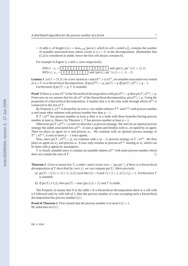
A distributed algorithm for the process number of a forest 7
• A tabletv of lengthL(tv) = maxw∈Rv(pn(w)) which in cell i, notedtv[i], contains the numberof unstable associated-trees whose vector is(i, i + 1) in the decomposition. (Remember that(1,2) is considered as stable, hence the first cell always contains 0).
For example in Figure 5,v andv1 store respectively:
HD(v) : tv = 0 0 3 2 3 1 0 0 1 and(pn(v),pn+(v)) = (2,2)
HD(v1): tv1 = 0 0 1 1 1 and(pn(v1),pn+(v1)) = (−1,−1)
Lemma 1 Let T = (V,E) be a tree rooted at r and aTw, r /∈ aTw, an unstable associated-tree rootedat w∈V in a hierarchical decomposition. Ifpn(aTw) = p, pn(T) = p iff pn(T\aTw) ≤ p−1.
Furthermore ifpn(T) = p, T is unstable.
Proof If there is a treeaTx in the hierarchical decomposition with pn(aTx) > p then pn(T\aTw) > p.From now on we assume that for allaTx of the hierarchical decomposition, pn(aTx) ≤ p. Using theproperties of a hierarchical decomposition, it implies that w is the only node through whichaTw isconnected to the rest ofT.
By Property 1,aTw is formed by its rootw, two stable subtreesTw1 andTw2 with process numberp and some other subtrees with process number less thanp−1.
If T \ aTw has process number at leastp thenw is a node with three branches having processnumber at leastp. Hence, by Theorem 1,T has process number at leastp+1.
Otherwise pn(T\aTw) < p and we describe ap-process strategy. We start by an optimal processstrategy the stable associated-treeaTw1. It usesp agents and finishes withw1 occupied by an agent.Then we place an agent onw and processw1. We continue with an optimal process strategy ofTw \aTw2, it uses at mostp−1 extra agents.
Now, since pn(T \aTw) < p, we continue with a(p−1)-process strategy ofT \aTw. We thenplace an agent onw2 and processw. It now only remains to processaTw2 starting atw2 which canbe done withp agents by assumption.
T is clearly unstable since it contains an unstable subtreeaTw with same process number whichdoes not contain the root ofT.
Theorem 2 Given a rooted tree T , a table t and a vector vect= (pn,pn+), if there is a hierarchicaldecomposition of T described by(vect,t), we can computepn(T). More precisely:
a) pn(T) = L(t) ⇔∃i ∈ [1..L(t)] such that t[i] = 0 and∀ j ∈ [i +1..L(t)] t[ j] = 1. Furthermore Tis unstable.
b) If pn(T) 6= L(t) thenpn(T) = maxpn,L(t)+1 and T is stable.
The Property a) means that if in the tablet of a hierarchical decomposition there is a cell witha 0 followed only by cells full of 1, then the process number ofa tree accepting such a hierarchicaldecomposition has process numberL(t).
Proof of Theorem 2 First remark that the process number is at mostL(t)+1.By induction onL(t).
RR n° 6560
inria
-002
8830
4, v
ersi
on 3
- 27
Jun
200
8

8 Coudert, Huc, Mazauric
(7,7)
(9,10)(7,7)(4,5)Tv4
v
(3,4) (3,4)
(2,2)
(3,4)
(6,7)(5,6)(4,5)(5,6)(9,10)(5,6)Tv5v Tv7
v Tv9v Tv10
v
Tv3vTv2
vTv1v
Tvv
Tv6v Tv8
v
⇔
Tv
Figure 6: A simpler hierarchical decomposition of the example of Figure 5.
• If L(t) = 0, T is a single node and pn(T) = 0. If L(t) = 1, T is a stable tree with vector(1,1) or (1,2). In both case pn(T) = 1. If L(t) = 2 andt[2] = 0, T is a stable tree with vector(2,2) and pn(T) = 2. If t[i] = 0 for all i ≤ L(t), T is a stable tree with vector(L(t),L(t)) andpn(T) = L(t).
• WhenL(t) ≥ 2 andt[L(t)] = 1. We call the associated-tree of the hierarchical decompositionhaving process numberL(t) aTw andw its root. By Lemma 1, pn(T) = L(t)⇔ pn(T\aTw)≤L(t)−1.
– If ∃i ∈ [1..L(t)] with t[i] = 0 and∀ j ∈ [i +1..L(t)] t[ j] = 1, we have pn(T \ aTw) ≤L(t)−1.
* Indeed, eithert[L(t)−1] = 1 and pn(T\aTw) = L(t)−1 by induction, so pn(T) =L(t).
* Or t[L(t)−1] = 0. In this case either, we have a table with only 0 and we are at aninitialisation case: pn(T\aTw) = L(t)−1 or we can delete this last cell, the lengthof the table is thenL(t)−2 and we are sure that pn(T\aTw) ≤ L(t)−1 by the veryfirst remark of the proof. In both cases we have once again pn(T) = L(t).
– If in t there is a cell with a number bigger than one followed by cellsfull of one until thelast cell, then, by induction, pn(T\aTw) = L(t) and hence pn(T) = L(t)+1.
• When L(t) ≥ 2 andt[L(t)] ≥ 2, we call one of the associated-tree of process numberL(t)aTw andw its root. pn(T \aTw) ≥ L(t), hence, from Lemma 1 pn(T) > L(t) which meanspn(T) = L(t)+1 by the very first remark.
T stable or unstable follows from Lemma 1 and the process strategy we described.
2.2 Minimal hierarchical decomposition
In the example of Figure 5, Theorem 2 directly says it has process number 9. If we now considerthis example minus the subtree of vector(9,10), then Theorem 2 says it has process number 7 andfurthermore that it is stable. Hence, we can get another hierarchical decomposition as shown onFigure 6.
INRIA
inria
-002
8830
4, v
ersi
on 3
- 27
Jun
200
8

A distributed algorithm for the process number of a forest 9
In fact we can generalize this simplification. Given a tablet and an indexi ≤ L(t), we notet[1..i]the table composed of thei first cells oft. For a given hierarchical decomposition described by itsvector and its table,HD = (vect, t), we callHDi = (vect,t[1..i]) a i-restricted hierarchical decom-position. Notice that ifHD is a hierarchical decomposition of a treeT, thenHDi is a hierarchicaldecomposition of the subtree composed of the associated-trees having process number at mosti.
A last definition, if a tree accepts several hierarchical decompositions, we say they areequivalent.We now describe the simplification of a given hierarchical decompositionHD = (vect,t) of a
treeT. If there is i ≤ L(t) such that a treeTi , whose hierarchical decomposition is described byHDi = (vect, t[1..i]), has process numberi + 1, thenHD is equivalent to a simpler hierarchicaldecompositionHD′ = ((i + 1, i + 1), t ′), whereL(t ′) = L(t), t ′[ j] = 0 for j ≤ i + 1, andt ′[ j] = t[ j]for j > i +1. If no suchi exist, the hierarchical decomposition can not be simplified.
We call a hierarchical decomposition we can not simplify aminimal hierarchical decomposition.Our algorithm will compute such decompositions for each subtreeTv, v∈V. Furthermore we have:
Lemma 2 Let HD= ((pn,pn+), t) be a minimal hierarchical decomposition. For all i∈ [2..L(t)],we have t[i] ∈ 0,1.
3 Distributed algorithm for the process number
We can now describe precisely algorithmalgoHD:
• The algorithm is initialized at the leaves. Each leaf sendsthe message((0,0), [ ]) (where[ ]represents a table of length 0) to its only neighbour which becomes its father.
• A nodev, which has received messages from all its neighbours but one, computes the minimalhierarchical decomposition ofTv using Algorithm 1. Then it sends(pn(Tv),pn+(Tv)), tv) toits last neighbour, its father.
• The last nodew receives a message from all its neighbours, it computes the minimal hierar-chical decomposition ofTv = T and Theorem 2 gives the process number pn(T). w is calledthe root ofT.
Remark It may happen that two adjacent nodesv andw receive a message from all their neighbors.It is the case when nodev, after sending its message to its last neighborw, receives a message fromw. In this case, bothv andw are potential candidates to be the root of the tree. There aretwopossibilities to solve this problem. If each node has a unique identifier (e.g. MAC address) knownby its neighbors, then the one ofv andw with the largest identifier becomes the root, otherwise,uandw send each other a random bit, repeat in case of equality, and the 1 win.
Lemma 3 Given a tree T= (V,E), with |V| = n, the time complexity of Algorithm 1 is O(logn).
Proof All operations are linear inL(tv), andL(tv) ≤ pn(T)≤ log3n.
RR n° 6560
inria
-002
8830
4, v
ersi
on 3
- 27
Jun
200
8

10 Coudert, Huc, Mazauric
Algorithm 1 Computation of the minimal hierarchical decompositionRequire: v1, ...,vd the visited neighbours of v, and the corresponding minimal hierarchical decom-
positionsHD(vi) = ((pn(vi),pn+(vi)), tvi )Require: t int
v , a table such thatt intv [i] := tv1[i]+ ...+ tvd−1[i], ∀i ∈ [2..max1≤ j≤d L(tvj )].
Require: Mv :=
vi ; ∀ j ∈ [1..d−1], pn(vj) ≤ pn(vi)
all vi such that pn(vi) is maximumEnsure: vect(v) andtv
computation 1: Let (pv, p+
v ) be the vector of the associated-tree ofv2: if ∀vi ∈ Mv, pn(vi) < 2 then Initial cases
3: (pv, p+v ) :=
(0,0) when∀vi ∈ Mv, pn(vi) = −1(1,1) when∀vi ∈ Mv, pn(vi) = 0(1,2) when|Mv| = 1 andvect(vi) = (1,1)(2,2) otherwise
4: elsegeneral cases5: if |Mv| = 2 then v is unstable6: (pv, p+
v ) := (pn(vi),pn(vi)+1), wherevi ∈ Mv
7: else v is stable8: if |Mv| > 2 then Theorem 19: (pv, p+
v ) := (pn(vi)+1,pn(vi)+1), wherevi ∈ Mv
10: else11: (pv, p+
v ) := (pn(vi),pn(vi)), wherevi ∈ Mv
computation of the table12: L(tv) := max
L(t intv ), pv
13: tv := t intv
14: if pv < p+v andpv > 1 then
15: tv[pv] := tv[pv]+116: tv[ j] := 0,∀ j ∈ [2..pv−1]17: (pv, p+
v ) := (−1,−1) Here, (pv, p+v ) is stable
18: Let k be such thattv[k] > 1 andtv[i] ≤ 1,∀i ∈ [k+1..L(tv)]19: Let k1 be such thattv[k1] = 0 andtv[i] = 1,∀i ∈ [k..k1−1]20: if tv[pv] = 0 then21: k2 := pv
22: else23: Let k2 be such thattv[k2] = 0 andtv[i] > 0, ∀i ∈ [pv..k2 −1] We assume that there exists a
virtual cell tv[L(tv)+1] = 024: if k,k1 andk2 exist then25: tv[i] := 0,∀i ∈ [2..max(k1,k2)] := 026: vect(v) := (max(k1,k2),max(k1,k2))27: elsethe hierarchical decomposition is already minimal28: vect(v) := (pv, p+
v )
INRIA
inria
-002
8830
4, v
ersi
on 3
- 27
Jun
200
8

A distributed algorithm for the process number of a forest 11
Lemma 4 Given a tree T= (V,E), with |V| = n, algo HD computespn(T) in n steps and overallO(nlogn) operations.
Proof Each nodev of degreedv has to computeMv (the set of neighborsvi with maximum pn(vi))which requiresO(dv) operations, andtsum
v (the sum of all received tables) that isO(∑d1 L(tsum
v ))operations. Finally it applies Algorithm 1. As∑v∈V dv = 2(n− 1), we have∑v∈V(dv + logn+
∑d1 L(tsum
v )) = O(nlogn).
Lemma 5 Given a tree T= (V,E), with |V|= n,algoHD sends n−1 messages each of sizelog3n+2.
Proof Nodev sends its minimal hierarchical decomposition to its father, that isHDv = (vect(v),tv),with vect(v) = (pn(v),pn+(v)). From Theorem 1 we know thatL(tv) ≤ log3 n, from Lemma 2,tvcontains only 0 and 1’s, hence we need only log3n bits to transmittv. Furthermore, if pn(v) ≥ 1,tv[pn(v)] = 0 and∀i ≤ pn(v), tv[i] = 0. Hence we can add an artificial 1 to the cell oftv with indexpn(v) to indicate the value pn(v).
To summarize, we transmit a tablet and two bitsab. ab= 00 meansvect(v) = (−1,−1), ab= 01meansvect(v) = (0,0), 10 meansvect(v) = (pn,pn) and 11 meansvect(v) = (pn,pn+ 1). Whena = 1, pn is the index of the first 1 in the transmitted table andtv is the transmitted table minus this1. Whena = 0, tv is the transmitted tablet. It is clear that in this coding, each message has sizelog3n+2.
4 Dynamic and incremental algorithms
In this section, we propose a dynamic algorithm that allows to compute the process number of thetree resulting of the addition of an edge between two trees. It also allows to delete any edge. To dothis efficiently, it uses one of the main advantage of the hierarchical decomposition: the possibilityto change the root of the tree without additional information (Lemma 6). From that we design anincremental algorithm that computes the process number of atree.
If we want to join two trees with an edge between their roots then it is easy to see that Algorithm 1will do it. However if we do not join them through the root, a preprocessing to change the root of thetrees needs to be done. In next Section we propose one. To apply this algorithm, each node needs tostore the information received from each of its neighbors and a table which is the sum of the receivedtables:∀vi ∈ Γ(v)∩Tv : vectvi , tvi andtsum
v . Recall thattsumv is defined astsum
v [ j] = ∑vi∈Γ(v)∩Tv tvi [ j] inthe algorithm.
For a given treeT, we noteD(T) or D if there is no ambiguity thediameterof T.We describe now three functions we will use in the dynamic version of our algorithm.
4.1 Functions for updating the process number
Lemma 6 (Change of the root)Given a tree T= (V,E) rooted at r1 ∈ V of diameter D, and itshierarchical decomposition, we can choose a new root r2 ∈ V and update accordingly the hierar-chical decomposition in O(D) steps of time complexity O(logn) each, using O(D) messages of sizelogn+3.
RR n° 6560
inria
-002
8830
4, v
ersi
on 3
- 27
Jun
200
8

12 Coudert, Huc, Mazauric
Proof We describe an algorithm to change the root fromr1 to r2:First,r2 sends a message tor1 through the unique path betweenr1 andr2, r2 = u0,u1,u2, . . . ,uk =
r1, to notify the change. Then,r1 computes its hierarchical decomposition, considering that uk−1 isits father. We assume that each nodev stores the information received from its neighbours andtsum
v .r1 applies Algorithm 1 using all vectors stored butvectuk−1 andtsum
v − tvk−1. Then it sends a messageto uk−1.
After, uk−1 computes its hierarchical decomposition, considering that uk−2 is its father, and sendsa message touk−2. We repeat untilr2 receives a message fromu1. Finally, r2 computes the processnumber ofT and becomes the new root. We have a new hierarchical decomposition.
In this algorithm,ui substracts the tabletui−1 from tsumui
, and later addstui+1, computesMui andfinally applies Algorithm 1. Clearly, all computation requiresO(logn) operations. The messagesneed one more bit than in the previous algorithm to indicate whether a table has to be added orsubstracted.
Lemma 7 (Addition of an edge) Given two trees Tr1 = (V1,E1) and Tr2 = (V2,E2) respectivelyrooted at r1 and r2, we can add the edge(w1,w2),w1 ∈ V1 and w2 ∈ V2 and compute the processnumber of T= (V1∪V2,E1∪E2∪ (w1,w2)), in at most D steps.
Proof First we change the roots ofTr1 andTr2 respectively tow1 andw2 using Lemma 6. Then,w1
andw2 decide of a root (see Remark 3) which finally computes the process number ofT.
Lemma 8 (Deletion of an edge)Given a tree T= (V,E) rooted at r and an edge(w1,w2)∈E, afterthe deletion of edge(w1,w2), we can compute the process number of the two disconnected trees inat most D steps.
Proof W.l.o.g. we may assume thatw2 is the father ofw1. Let Tw1 be the subtree rooted atw1
andT \Tw1 the tree rooted atr. Remark that it includesw2. The process number ofTw1 is deducedfrom the previously computed hierarchical decomposition.Now, to compute the process number ofT \Tw1, we apply the change root algorithm and nodew2 becomes the new root ofT \Tw1.
4.2 Incremental algorithm
From Lemma 7, we obtain an incremental algorithm (IncHD) that, starting from a forest ofn discon-nected vertices with hierarchical decomposition((0,0,)[ ]), add tree edges one by one in any orderand updates the process number of each connected component.At the end, we obtain the processnumber ofT.
This algorithm is difficult to analyze in average, but the best and worst cases are straightforward:
• Worst case:T consists of two subtrees of sizen/3 and process number log3(n/3) linked viaa path of lengthn/3. Edges are inserted alternatively in each opposite subtrees. ThusIncHDrequiresO(n2) steps and messages, and overallO(n2 logn) operations
INRIA
inria
-002
8830
4, v
ersi
on 3
- 27
Jun
200
8
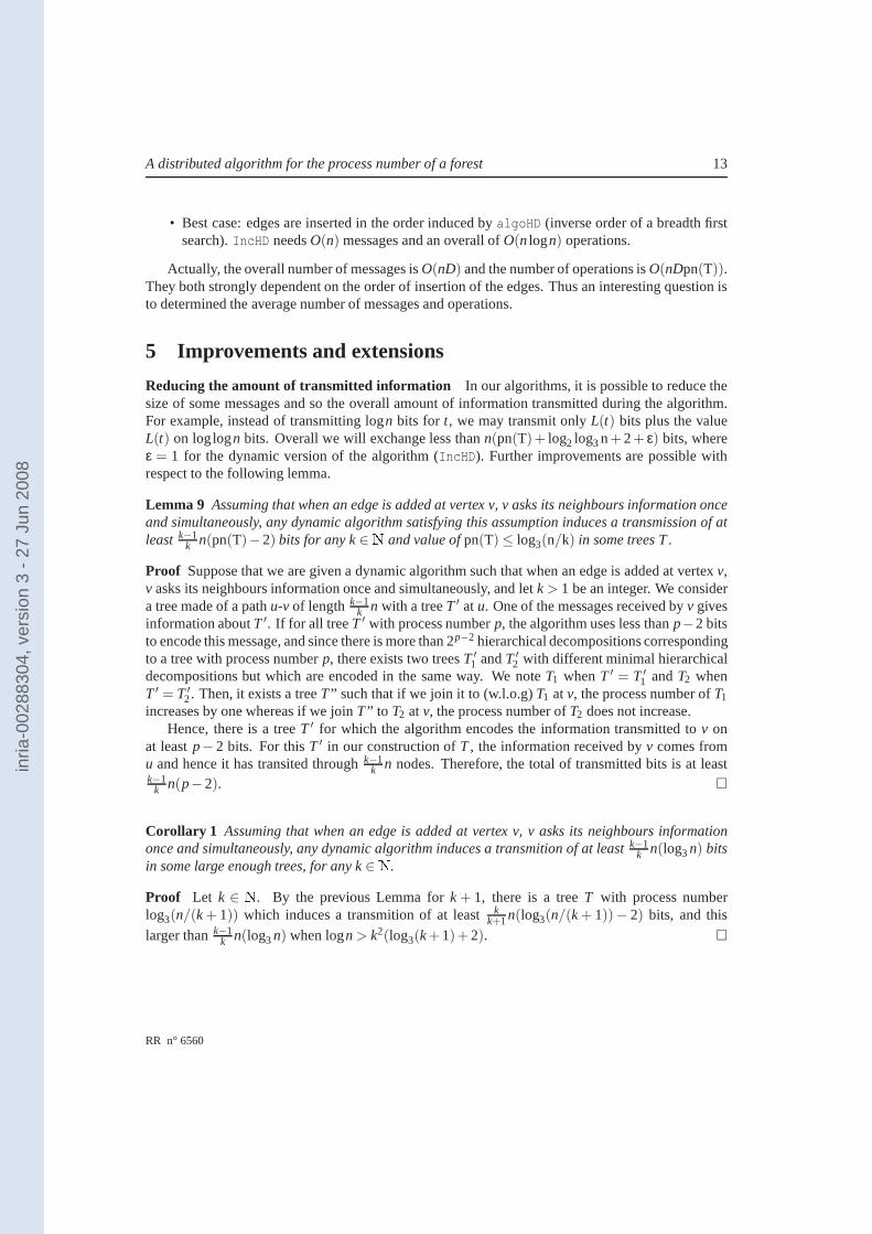
A distributed algorithm for the process number of a forest 13
• Best case: edges are inserted in the order induced byalgoHD (inverse order of a breadth firstsearch).IncHD needsO(n) messages and an overall ofO(nlogn) operations.
Actually, the overall number of messages isO(nD) and the number of operations isO(nDpn(T)).They both strongly dependent on the order of insertion of theedges. Thus an interesting question isto determined the average number of messages and operations.
5 Improvements and extensions
Reducing the amount of transmitted information In our algorithms, it is possible to reduce thesize of some messages and so the overall amount of information transmitted during the algorithm.For example, instead of transmitting logn bits for t, we may transmit onlyL(t) bits plus the valueL(t) on loglogn bits. Overall we will exchange less thann(pn(T)+ log2 log3n+2+ ε) bits, whereε = 1 for the dynamic version of the algorithm (IncHD). Further improvements are possible withrespect to the following lemma.
Lemma 9 Assuming that when an edge is added at vertex v, v asks its neighbours information onceand simultaneously, any dynamic algorithm satisfying thisassumption induces a transmission of atleast k−1
k n(pn(T)−2) bits for any k∈N and value ofpn(T) ≤ log3(n/k) in some trees T .
Proof Suppose that we are given a dynamic algorithm such that when an edge is added at vertexv,v asks its neighbours information once and simultaneously, and letk > 1 be an integer. We considera tree made of a pathu-v of length k−1
k n with a treeT ′ atu. One of the messages received byv givesinformation aboutT ′. If for all treeT ′ with process numberp, the algorithm uses less thanp−2 bitsto encode this message, and since there is more than 2p−2 hierarchical decompositions correspondingto a tree with process numberp, there exists two treesT ′
1 andT ′2 with different minimal hierarchical
decompositions but which are encoded in the same way. We noteT1 whenT ′ = T ′1 andT2 when
T ′ = T ′2. Then, it exists a treeT” such that if we join it to (w.l.o.g)T1 atv, the process number ofT1
increases by one whereas if we joinT” to T2 at v, the process number ofT2 does not increase.Hence, there is a treeT ′ for which the algorithm encodes the information transmitted to v on
at leastp−2 bits. For thisT ′ in our construction ofT, the information received byv comes fromu and hence it has transited throughk−1
k n nodes. Therefore, the total of transmitted bits is at leastk−1
k n(p−2).
Corollary 1 Assuming that when an edge is added at vertex v, v asks its neighbours informationonce and simultaneously, any dynamic algorithm induces a transmition of at leastk−1
k n(log3n) bitsin some large enough trees, for any k∈N.
Proof Let k ∈ N. By the previous Lemma fork + 1, there is a treeT with process numberlog3(n/(k+ 1)) which induces a transmition of at leastkk+1n(log3(n/(k+ 1))− 2) bits, and this
larger thank−1k n(log3n) when logn > k2(log3(k+1)+2).
RR n° 6560
inria
-002
8830
4, v
ersi
on 3
- 27
Jun
200
8

14 Coudert, Huc, Mazauric
Reducing the number of operations It makes no doubt that the worst case complexity ofIncHDand more specifically of Lemma 7 can be seriously improved. Inparticular, instead of changing theroots of both trees, we may change onlyr1 to w1, then transmit information in the direction ofr2,and eventually stop the transmissions beforer2 if the minimal hierarchical decomposition of somenode remains unchanged.
It is also interesting to notice that using arguments similar to [5], we can get a centralized algo-rithm using a linear number of operations.
Trees and forests of unknown size If the sizen of the tree is unknown, a node encodes each bit ofthe transmitted tablet on 2 bits, that is 00 for 0 and 01 for 1. It allows to use 11 to codethe end of thetable and hence to know its length. Thus the receiver may decode the information without knowingn. In this coding the table requires 2L(t)+ 2 bits and the transmission requires 2L(t)+ 4+ ε bits,whereε = 1 for IncHD and 0 foralgoHD. Remember thatL(t) ≤ pn(T).
Computing other parameters Our algorithms can be adapted to compute the node search numberor the pathwidth of any tree with the same time complexity andtransmission of information. Forthat, it is sufficient to change the values of the initial cases (lines 1 and 1) in Algorithm 1.
For the node search number we would use the initial cases of the left of Figure 5. Notice that inthis case we do not use the vector(1,2).
if ∀vi ∈ Mv, pn(vi) < 2 then
(pv, p+v ) :=
(1,1) when∀vi ∈ Mv, pn(vi) = −1(2,2) otherwise
if ∀vi ∈ Γ(v), pn+(vi) < 2 then
(pv, p+v ) :=
(0,0) when|Mv| = 0(1,1) when|Mv| = 1(1,2) when|Mv| = 2(2,2) otherwise
Figure 7: Initial cases for node search number (left) and edge search number (right).
For the edge search number of a tree, we can prove that ns(T)− 1≤ es(T) ≤ ns(T), whereason a general graph we only have ns(T)− 1 ≤ es(T) ≤ ns(T) + 1. To adapt Algorithm 1 for theedge search number, we would use the initial cases of the right of Figure 5 plus the extra rule thatall received vectors(1,2) are interpreted as if they were vectors(2,2). Also, if all received vectorsverifies pn+(vi) < 2, Mv is the set of all received vectors different from (-1,-1). Notice that it givesthe first algorithm to compute the edge search number of trees.
Algorithm algoHD has been implemented for the process number, the node searchnumber andthe edge search number, as well as corresponding search strategies [1].
About the difference of the parameters Finally, the following lemma characterizes the trees forwhich the process number (resp. edge search number) equals the pathwidth.
Lemma 10 Given a tree T ,pn(T) = pw(T)+1 = p+1 (resp.pn(T) = es(T)+1 = p+1) iff thereis a node v such that any components of T−v has pathwidth at most p and there is at least threecomponents with process number (resp. edge search number) pof which at most two have pathwidthp.
INRIA
inria
-002
8830
4, v
ersi
on 3
- 27
Jun
200
8
A distributed algorithm for the process number of a forest 15
This lemma means that the difference between, e.g., the process number and the pathwidth comesfrom the difference on trees with smaller parameter and ultimately from trees with those parametersequal to 1 or 2.
To give such characterisations for more general classes of graphs remains a challenging problem.
Acknowledgments
We would like to thanks Nicolas Nisse and Hervé Rivano for fruitfull discussions on this problem.
References
[1] http://www-sop.inria.fr/members/Dorian.Mazauric/Capture/index.php.htm.
[2] D. Coudert, S. Perennes, Q.-C. Pham, and J.-S. Sereni. Rerouting requests in wdm networks.In AlgoTel’05, pages 17–20, Presqu’île de Giens, France, mai 2005.
[3] D. Coudert and J-S. Sereni. Characterization of graphs and digraphs with small process num-ber. Research Report 6285, INRIA, September 2007.
[4] J. Díaz, J. Petit, and M. Serna. A survey on graph layout problems.ACM Computing Surveys,34(3):313–356, 2002.
[5] J.A. Ellis, I.H. Sudborough, and J.S. Turner. The vertexseparation and search number of agraph.Information and Computation, 113(1):50–79, 1994.
[6] F. V. Fomin and D. Thilikos. An annotated bibliography onguaranteed graph searching.The-oretical Computer Science, Special Issue on Graph Searching, 2008, to appear.
[7] N. G. Kinnersley. The vertex separation number of a graphequals its pathwidth.Inform.Process. Lett., 42(6):345–350, 1992.
[8] M. Kirousis and C.H. Papadimitriou. Searching and pebbling. Theor. Comput. Sci., 47(2):205–218, 1986.
[9] N. Megiddo, S. L. Hakimi, M. R. Garey, D. S. Johnson, and C.H. Papadimitriou. The com-plexity of searching a graph.J. Assoc. Comput. Mach., 35(1):18–44, 1988.
[10] T. D. Parsons. Pursuit-evasion in a graph. InTheory and applications of graphs, pages 426–441. Lecture Notes in Math., Vol. 642. Springer, Berlin, 1978.
[11] N. Robertson and P. D. Seymour. Graph minors. I. Excluding a forest.J. Combin. Theory Ser.B, 35(1):39–61, 1983.
[12] P. Scheffler. A linear algorithm for the pathwidth of trees. In R. Henn R. Bodendiek, editor,Topics in Combinatorics and Graph Theory, pages 613–620. Physica-Verlag Heidelberg, 1990.
RR n° 6560
inria
-002
8830
4, v
ersi
on 3
- 27
Jun
200
8

16 Coudert, Huc, Mazauric
[13] K. Skodinis. Construction of linear tree-layouts which are optimal with respect to vertex sepa-ration in linear time.J. Algorithms, 47(1):40–59, 2003.
INRIA
inria
-002
8830
4, v
ersi
on 3
- 27
Jun
200
8
Unité de recherche INRIA Sophia Antipolis2004, route des Lucioles - BP 93 - 06902 Sophia Antipolis Cedex (France)
Unité de recherche INRIA Futurs : Parc Club Orsay Université- ZAC des Vignes4, rue Jacques Monod - 91893 ORSAY Cedex (France)
Unité de recherche INRIA Lorraine : LORIA, Technopôle de Nancy-Brabois - Campus scientifique615, rue du Jardin Botanique - BP 101 - 54602 Villers-lès-Nancy Cedex (France)
Unité de recherche INRIA Rennes : IRISA, Campus universitaire de Beaulieu - 35042 Rennes Cedex (France)Unité de recherche INRIA Rhône-Alpes : 655, avenue de l’Europe - 38334 Montbonnot Saint-Ismier (France)
Unité de recherche INRIA Rocquencourt : Domaine de Voluceau- Rocquencourt - BP 105 - 78153 Le Chesnay Cedex (France)
ÉditeurINRIA - Domaine de Voluceau - Rocquencourt, BP 105 - 78153 Le Chesnay Cedex (France)
http://www.inria.fr
ISSN 0249-6399
inria
-002
8830
4, v
ersi
on 3
- 27
Jun
200
8

Pathwidth of outerplanar graphs ∗
David Coudert, Florian Huc and Jean-Sebastien SereniMASCOTTE, I3S-CNRS–INRIA–UNSA
2004 route des Lucioles – BP9306902 Sophia Antipolis, FRANCE
E-mail: [email protected]
Abstract
We are interested in the relation between the pathwidth of a biconnected outerplanar graphand the pathwidth of its (geometric) dual. Bodlaender and Fomin [3], after having proved thatthe pathwidth of every biconnected outerplanar graph is always at most twice the pathwidth ofits (geometric) dual plus two, conjectured that there exists a constant c such that the pathwidth ofevery biconnected outerplanar graph is at most c plus the pathwidth of its dual. They also conjec-tured that this was actually true with c being one for every biconnected planar graph. Fomin [10]proved that the second conjecture is true for all planar triangulations. First, we construct for eachp ≥ 1 a biconnected outerplanar graph of pathwidth 2p+1 whose (geometric) dual has pathwidthp+1, thereby disproving both conjectures. Next, we also disprove two other conjectures (one ofBodlaender and Fomin [3], implied by one of Fomin [10]). Finally we prove, in an algorithmicway, that the pathwidth of every biconnected outerplanar graph is at most twice the pathwidth ofits (geometric) dual minus one. A tight interval for the studied relation is therefore obtained, andwe show that all cases in the interval happen.
1 Introduction
A planar graph is a graph that can be embedded in the plane without crossing edges. It is said to beouterplanar if it can be embedded in the plane without crossing edges and such that all its verticesare incident to the unbounded face. For any graph G, we denote by V (G) its vertex set and by E(G)its edge set. The dual of the planar graph G, denoted by G∗, is the graph obtained by putting onevertex for each face, and joining two vertices if and only if the corresponding faces are adjacent.The weak dual of G, denoted by TG, is the induced subgraph of G∗ obtained by removing the vertexcorresponding to the unbounded face. As is well known, the weak dual of an outerplanar graph isa forest, and the weak dual of a biconnected outerplanar graph is a tree. Furthermore, linear-timealgorithms to recognise and embed outerplanar graphs are known (see for instance [15, 21]). Notethat the dual of a planar graph can also be computed in linear-time.
The notion of pathwidth was introduced by Robertson and Seymour [17]. A path decompositionof a graph G = (V,E) is a set system (X1, . . . ,Xr) of V such that
(i)⋃r
i=1 Xi = V ;
(ii) ∀xy ∈ E,∃i ∈ 1,2, . . . ,r : x,y ⊂ Xi;
∗This work was partially funded by the European projects IST FET AEOLUS and COST 293 GRAAL, and done withinthe CRC CORSO with France Telecom R&D.
1

(iii) ∀(i0, i1, i2) ∈ 1,2, . . . ,r3, i0 < i1 < i2 ⇒ Xi0 ∩Xi2 ⊆ Xi1 .
The width of the path decomposition (X1, . . . ,Xr) is max1≤i≤r |Xi|− 1. The pathwidth of G, denotedby pw(G), is the minimum width over its path decompositions.
The pathwidth of a graph was shown to be equal to its vertex separation [12]: a layout (or vertex-ordering) L of a graph G = (V,E) is a one-to-one correspondence between V and 1, . . . , |V |. Thevertex separation of (G,L) is max1≤i≤|V | |M(i)| where
M(i) := v ∈V : L(v) > i and ∃u ∈ N(v) : L(u) ≤ i.
The vertex separation of G, denoted by vs(G), is the minimum of the vertex separation of (G,L)taken over all vertex-orderings L.
Computing the pathwidth of graphs is an active research area, in which a lot of work has beendone (survey papers are for instance [6, 2, 16]). It was shown [4] that the pathwidth of graphs withbounded treewidth can be computed in polynomial time. As outerplanar graphs have treewidth two,the pathwidth of an outerplanar graph is polynomially computable. However, the exponent in therunning time of the algorithm is rather large, so the algorithm is not useful in practice. This is whyGovindan et al. [11] gave an O(n log(n)) time algorithm for approximating the pathwidth of outer-planar graphs with a multiplicative factor of three. For biconnected outerplanar graphs, Bodlaenderand Fomin [3] improved upon this result by giving a linear-time algorithm which approximates thepathwidth of biconnected outerplanar graphs with a multiplicative factor two (and a correspondingpath decomposition is obtained in time O(n log(n))). To do so, they exhibited a relationship betweenthe pathwidth of an outerplanar graph and the pathwidth of its dual. More precisely, the followingholds.
Theorem 1 (Bodlaender and Fomin [3]) Let G be a biconnected outerplanar graph without loopsand multiple edges. Then pw(G∗) ≤ pw(G) ≤ 2pw(G∗)+2.
Observe that adding a vertex linked to all other vertices of any graph increases its pathwidth byexactly one. Since the weak dual of an outerplanar graph (which can be computed in linear-time) isa tree and there exist linear-time algorithms to compute the pathwidth of a tree [8], this yields thedesired approximation (obtaining a corresponding path decomposition needs more work).
Bodlaender and Fomin [3] suggested that a stronger relationship holds between the pathwidth ofa planar graph and the pathwidth of its dual.
Conjecture 1 (Bodlaender and Fomin [3]) There is a constant c such that for every biconnectedouterplanar graph G without loops and multiple edges pw(G) ≤ pw(G∗)+ c.
Conjecture 2 (Bodlaender and Fomin [3]) For every biconnected planar graph G without loopsand multiple edges, pw(G) ≤ pw(G∗)+1.
Fomin [10] proved that if G is any biconnected planar graph of maximum degree at most three,then pw(G) ≥ pw(G∗)−1. This implies that Conjecture 2 is true for every planar triangulation, sinceany planar triangulation is the dual of a biconnected planar graph of maximum degree three.
It is worth noting that these conjectures are motivated by the following result about the treewidth,conjectured by Robertson and Seymour [18] and proved by Lapoire [13] using algebraic methods(notice that Bouchitte, Mazoit and Todinca [5] gave a shorter and combinatorial proof of this result).
Theorem 2 (Lapoire [13]) For every planar graph G, tw(G) ≤ tw(G∗).
2

In Section 2, we exhibit a family (Gp)p≥1 of biconnected outerplanar graphs with maximumdegree four such that pw(Gp) = 2p + 1 and pw(G∗
p) = p + 1, thereby disproving both conjectures.To construct these graphs, we introduce a general construction which actually allows us to prove thefollowing result.
Theorem 3 For every integer p ≥ 1 and every integer k ∈ 1,2, . . . , p+1, there exists a biconnectedouterplanar graph of pathwidth p+ k whose weak dual has pathwidth p.
Let us mention here that Fomin and Thilikos [9] also disproved, independently, Conjecture 1.Next, we disprove the following conjecture of Bodlaender and Fomin [3].
Conjecture 3 (Bodlaender and Fomin [3]) For every simple 2-connected planar graph G, pw(G)≥pw(G∗)−1.
In Section 3, we prove the following result which improves the upper bound given by Theorem 1.
Theorem 4 Let G be a biconnected outerplanar graph without loops and multiple edges. Thenpw(G) ≤ 2pw(G∗)−1.
As a consequence, the previous approximation for the pathwidth of biconnected outerplanargraphs is also improved. We give an algorithmic proof which allows to obtain a layout of the out-erplanar graph G considered (and whose vertex separation is hence at most 2pw(G)−1).
Furthermore, Theorem 3 shows that this bound is best possible in general.
2 Counter-examples
In this section, we establish Theorem 3 and deduce the following corollary which disproves Conjec-tures 1 and 2.
Corollary 1 For every integer p ≥ 1, there exists a triangle-free biconnected outerplanar graph G p
of maximum degree four whose pathwidth is 2p+1 such that the pathwidth of its dual is p+1.
For each i ∈ 1,2,3,4, let Hi be a biconnected outerplanar graph of pathwidth p whose weakdual has pathwidth p′. We shall describe a construction which yields a biconnected outerplanar graphC (H1,H2,H3,H4) of pathwidth p + 2 whose weak dual has pathwidth p′ + 1. This construction willbe illustrated by examples yielding the graphs Gp of Corollary 1.
A 4-cycle is called a square. Two squares are adjacent if they share exactly one edge. The degreeof the square S is the number of squares adjacent to S. Let the cross K be the biconnected outerplanargraph consisting of four squares of degree one and one square of degree four (see Figure 1(a)).
For each i ∈ 1,2,3,4, let xiyi be an edge of Hi incident to the unbounded face in an outerplanarembedding of Hi. This edge is chosen such that there exists an optimal layout L of THi where the vertexv corresponding to the the bounded face incident to xiyi fulfils L(v) = |V (THi)| for i ∈ 2,3. Noticethat this is always possible, and directly follows from Theorem 6 cited in Section 3. For i ∈ 1,2,we denote by Li an optimal layout of Hi, i.e. a layout with vertex separation p, and without loss ofgenerality we assume that Li(xi) < Li(yi).
Consider the cross K of Figure 1(a). For each i ∈ 1,2,3,4, the edge ei of K is identified withthe edge xiyi. We assume moreover that the vertices x1 and x2 are identified with the vertices u1
and u2 respectively (see Figure 1(b)). Notice that there is generally not a unique way to achieve this
3

β
δ
α
γ
u2
v2
v1 u1
e2
e4
e3
e1
(a) The cross K.
x1 = u1
x2 = u2
H2
H1
H3
H4
(b) Gluing four graphs H1,H2,H3,H4 onthe cross K
Figure 1: When identifying the edges, we ensure that x1 is identified with u1 and x2 with u2.
construction, but we shall denote by C (H1,H2,H3,H4) any graph obtained from H1,H2,H3,H4 in thisway.
It is clear by the construction that any such graph C (H1,H2,H3,H4) is a biconnected outerplanargraph. As an example, let G1 be the biconnected outerplanar graph consisting of three squares ofdegree one and one square of degree three (see Figure 2). For any integer p ≥ 2, let G p be the graphC (Gp−1,Gp−1,Gp−1,Gp−1), obtained as indicated in Figures 3 and 4. Remark that the condition onthe vertices x1 and x2 is clearly fulfilled in this case thanks to the symmetry of the graphs G p, and thatthe maximum degree of Gp is four.
(a) G1 and G∗1 (b) G1 and TG1
Figure 2: G1, graph consisting of one square of degree three and three squares of degree one, the dualG∗
1 and the weak dual TG1 , a star.
In the following three lemmata, we prove the announced properties of the construction. Thecentral square of the cross is denoted by S, and the corresponding vertex of the dual is s.
4
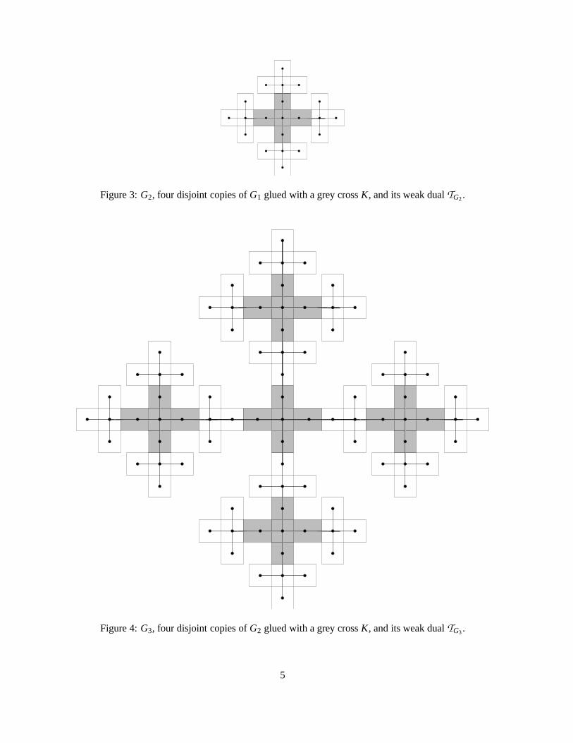
Figure 3: G2, four disjoint copies of G1 glued with a grey cross K, and its weak dual TG2 .
Figure 4: G3, four disjoint copies of G2 glued with a grey cross K, and its weak dual TG3 .
5

Lemma 1 For each i ∈ 1,2,3,4, let Hi be a biconnected outerplanar graph whose weak dual Ti haspathwidth p ≥ 1. The pathwidth of the weak dual of graph C (H1,H2,H3,H4) is p+1.
We introduce the following definition: for every vertex v of a tree T , a branch at v is any maximalsubtree which contains a neighbour of v without containing v. The following result will be useful toprove Lemma 1.
Theorem 5 (Scheffler [19]) For every integer p ≥ 1 and every tree T , pw(T ) ≥ p + 1 if and only ifthere exists a vertex t of T with at least three branches of pathwidth at least p.
Proof of Lemma 1. By induction on p ≥ 1, the result being true for p = 1. If the pathwidth ofeach tree Ti is p, it is not difficult to construct a layout L of the weak dual of C (H1,H2,H3,H4) withvertex separation p+1: first, label the vertices of Ti according to an optimal layout of T1. Then, labelthe vertex s1, i.e. define L(s1) := |V (T1)|+ 1. Next, label the vertices of T2 (from L(s1) + 1 up toL(s1) + |V (T2)|) according to an optimal layout of T2 such that the unique neighbour of s2 in T2 isgiven the biggest integer (such a layout exists by the construction). The next vertex to be labelled iss2, and an analoguous labeling is done for the vertices of T3 and s3. Finally, the vertex s est labelled,then the vertices of T4 (according to an optimal layout of T4) and last the vertex s3.
Also, the pathwidth of the weak dual of C (H1,H2,H3,H4) is more than p by Theorem 5 since thevertex s has four branches with pathwidth p.
Lemma 2 For each i ∈ 1,2,3,4, let Hi be a biconnected outerplanar graph of pathwidth p ≥ 1.The vertex separation of the graph C (H1,H2,H3,H4) is at least p+2.
Proof. Consider any layout L of H := C (H1,H2,H3,H4). We shall prove that the vertex separationof (H,L) is at least p + 2. The subgraph of H induced by removing the vertices of the square S isthe disjoint union of the four graphs H1,H2,H3 and H4, each of them having pathwidth p. Note thatthe roles played by those four graphs in this proof are symmetric. Assume that the vertex a such thatL(a) = 1 and the vertex b such that L(b) = |V (H)| are in V (H1)∪V (S) and V (H1)∪V (H2)∪V (S)respectively. By hypothesis, there exists i∈L(V (H4)) such that there are p vertices x of H4 with L(x) >i, each having a neighbour y in H4 with L(y)≤ i. As a similar integer exists for H3, we suppose withoutloss of generality that there exists a vertex v ∈V (H3) with L(v) > i. Let X := ∪3
j=1V (H j)∪V (S). Saythat a vertex x ∈ X is an m-vertex if L(x) < i and an M-vertex if L(x) > i. In particular, a is an m-vertexand b and v are M-vertices. An edge is bad if it links an m-vertex to an M-vertex. A bad pair is a pairof bad edges that are either disjoint, or incident to the same m-vertex. Denote by Q the subgraph of Ginduced by X , and note that the existence of a bad pair in Q implies that vs(H,L)≥ vs(H4)+2 = p+2.
Remark now that Q is 2-connected, so according to the Fan Lemma, there exists in Q two pathsP1 and P2 respectively from a to b and from a to v, which are vertex-disjoint except in a. Note that P1
and P2 are both disjoint from H4. As a in an m-vertex and b and v are M-vertices, there exists a badedge on P1 and a bad edge on P2, which necessarily from a bad pair (since the only common vertex ofP1 and P2 is a, an m-vertex). Therefore, the vertex separation of (H,L) is at least p+2.
Lemma 3 For each i ∈ 1,2,3,4, let Hi be a biconnected outerplanar graph of pathwidth p ≥ 1.The pathwidth of C (H1,H2,H3,H4) is at most p+2.
Proof. We shall construct a layout of C (H1,H2,H3,H4) from optimal layouts Li of Hi, i ∈ 1,2,3,4.Start by labelling all the vertices of H4 according to L4. The vertex separation never exceeds p + 2,
6

since the only unlabelled vertices not in H4 that might have labelled neighbours are β and γ. By theconstruction, the optimal layout L1 of H1 can be chosen such that L1(x1) < L1(y1). Label the verticesof H1 until the vertex x1 is labelled. As previously, the vertex separation does not exceed p+2 whendoing so. Now, label the vertex β, which does not change the vertex separation, as β has exactly oneunlabelled vertex, α. Now go on labelling the vertices of H1 according to L1. The vertex-separationstill does not exceed p + 2, the only unlabelled vertices not in H1 with labelled neighbours beingα and γ. By the construction again, the layout L2 of H2 can be chosen such that L2(x2) < L2(y2).Therefore we can apply the same procedure to label the vertices of H2: first label them until x2 islabelled, then label the vertex α and finish labelling the vertices of H2. At last, label the vertices of H3
(the vertex separation does not exceed p + 2 when doing so, since the only unlabelled vertices withlabelled neighbours not in H3 are δ and γ), and then label the vertices δ and γ. The obtained layout hasvertex separation at most p+2.
Proof of Theorem 3. The proof is by induction on p ≥ 1. If p = 1, two adjacent squares and G1 givethe desired result when k = 1 and k = 2 respectively.
Suppose that the result is true for p−1 ≥ 1, and let k ∈ 1,2, . . . , p+1. First, let k = 1: as is wellknown, there exist biconnected outerplanar graphs of pathwidth p+1 whose weak dual has pathwidthp. If k ∈ 2,3, . . . , p + 1, then k− 1 ∈ 1,2, . . . , p so, by the induction hypothesis, there exists abiconnected outerplanar H of pathwidth (p−1)+(k−1) whose weak dual has pathwidth p−1. Thenby Lemmata 1, 2 and 3, C (H,H,H,H) has pathwidth p + k and its weak dual has pathwidth p, asdesired.
Now we show how the family (Gp)p≥1 can be used to also disprove Conjecture 3.First, observe that the pathwidth of a multigraph G is equal to the pathwidth of its underlying
simple graph, denoted U(G).Let uv be an edge of a 2-connected planar graph G. Denote F1 and F2 the two faces incident to uv,
and f1 and f2 the corresponding vertices of G∗. To subdivide i times the edge uv (i.e. to replace it byan induced path of length i+1) leads to replace the edge f1 f2 in G∗ by i+1 parallel edges.
Now, consider Gp and an embedding of G∗p such that G∗∗
p ' Gp. Call o the vertex correspondingto the external face of Gp in G∗
p. Let Hp be the grah obtained by subdividing each edge of G∗p incident
to o (i.e. by replacing it by an induced path of length two). Notice that Hp is a simple 2-connectedplanar graph. According to the preceding remarks, U(H ∗
p) ' Gp, and hence pw(H∗p) = pw(Gp).
For every face F of Gp, let m(F) be the number of edges of F incident to the unbounded face. Letm := maxF(m(F)).
Lemma 4 pw(Hp) ≤ pw(G∗p)+m = pw(G∗
p)+3
Proof. It is clear by the definition of Gp that m = 3. Let l be an optimal layout of G∗p (i.e. a layout
of minimum vertex-separation), and let construct a layout of Hp of width at most pw(G∗)+m. Let uslabel every vertex v belonging to both Hp and G∗
p with (l(v),0). Now, if the vertex labelled (l(v),0)has j unlabelled neighbours, label them (l(v),1), · · · ,(l(v), j). The obtained labeling surely has vertexseparation at most pw(G∗
p)+m.
If Conjecture 2 is true, then pw(Hp) ≥ pw(H∗p) − 1 = pw(Gp) − 1. However, by lemma 4,
pw(Hp) ≤ pw(G∗p)+3 and so pw(G∗
p)+3 ≥ pw(Gp)−1 which is false for p > 6.
7

3 Upper bound
We shall present in this section an algorithm which, given a biconnected outerplanar graph G, com-putes a layout of G with vertex separation at most 2pw(TG)+ 1. As pw(TG) = pw(G∗)− 1 for anybiconnected outerplanar G (see [3]), this establishes Theorem 4.
First, recall that a caterpillar is a tree in which a single path, the spine, is incident to (or contains)every edge. The caterpillars are the only trees of pathwidth one: every caterpillar has surely pathwidthone, and if a tree T is not a caterpillar, then it contains a spider with three legs of length two (seeFigure 5). But such a tree has pathwidth at least two by Theorem 5.
Figure 5: A spider with three legs of length two.
Proposition 1 Let G be a biconnected outerplanar graph whose weak dual is a caterpillar. Then Ghas pathwidth at most three.
Proof. Here is a layout of the vertices of G with vertex separation at most three. Let P := v1v2 . . .vk
be a longest path of TG. Denote by Fi the face of G corresponding to the vertex vi, i ∈ 1,2, . . . ,k.Label by 1 a vertex v of F1 of degree two (such a vertex exists as G is outerplanar and v1 is a leaf ofT ). Then recursively label every vertex of F1 of degree two which is adjacent to a labelled vertex.
Now, apply the following procedure in which we suppose that V (Fi−1)∩V (Fi) = xi,yi andV (Fi)∩V(Fi+1) = xi+1,yi+1, see Figure 6.
Fi−1 Fi+1Fi
xi+1
yi+1
w2
w3
u1yi
w1
xi
Figure 6: Vertices for step i.
1: for i = 2 to k−1 do2: let P := xiw1 . . .w jxi+1 be the path of G from xi to xi+1 consisting of edges incident to the
unbounded face. Label the vertices of P from xi to wk
3: let P′ := yiu1 . . .ut yi+1 be the path of G from yi to yi+1 consisting of edges incident to theunbounded face. Label the vertices of P′ from yi to ut
4: end forLast, label the vertices clockwise from xk to yk.The obtained layout surely has vertex separation at most three.
The procedure given in the preceding proof actually achieves an optimal layout of the correspond-ing graph. Indeed, such a graph has pathwidth two if its weak dual is path, and pathwidth threeotherwise. Note also that the time complexity of the procedure is linear.
We will use the following result about the pathwidth of trees.
8

Theorem 6 (Ellis, Sudborough and Turner [8]) For any tree T , and any integer p ≥ 2, pw(T ) ≤ pif and only if there is a path P such that every connected component of the forest induced by thevertices of V (T )\V (P) has pathwidth at most p−1.
We consider the recursive procedure given by Algorithm 1. It computes a layout of G stored inthe list l, which is initialised by l(v) := ∞ for every vertex v ∈ V (G) (this means that all vertices areunlabelled at the beginning).
Notice that what is done in lines 16–17 and 32–33 is equivalent to label all the vertices of H excepty (or y′ respectively), and to keep s updated.
The following lemma suffices to establish Theorem 4.
Lemma 5 For any biconnected outerplanar graph G whose weak dual T has pathwidth p, the proce-dure Layout of Algorithm 1 returns a layout with vertex separation at most 2p+1.
Proof. Algorithm 1 clearly assigns a unique label to every vertex of G.For the vertex separation of the obtained layout, the proof is by induction on the pathwidth p of
T . If p is one, then T is a caterpillar and Proposition 1 gives the conclusion.Suppose now that for every biconnected outerplanar graph whose weak dual has pathwidth at most
p−1 ≥ 1, the procedure Layout of Algorithm 1 returns a layout with vertex separation at most 2p−1.Let us prove that the obtained layout for G has pathwidth at most 2p+1.
Stop the labelling of G at any moment and denote by F the set of unlabelled vertices with alabelled neighbour. If no subgraph H has been labelled yet, then the set F consists of x and x ′, so itssize is at most 2p+1. If a subgraph H has just been labelled, then F consists of two vertices, namelyx′ and y or x and y′.
Suppose now that a subgraph H is being labelled. Without loss of generality, say that its intersec-tion with the current face Fi is x,y. There is only one vertex of F not in H , namely x′. Therefore, if|F ∩V (H)| ≤ 2p we have |F | ≤ 2p+1 as wanted. As the vertex separation of the layout used to labelH is at most 2p− 1, the only problem that might occur is if |F ∩ (V (H) \ x,y)| = 2p− 1, and x,x ′
and y also belong to F . This implies that y was requested to be labelled in the original layout l usedfor H , but kept unlabelled as indicated in the algorithm. But in this case, in the labelling l of H , thevertex x is unlabelled, and has at least a labelled neighbour, y. So the number of unlabelled vertices ofH with a labelled neighbour in H is |F ∩ (V (H)\x,y)|+1 = 2p, a contradiction.
As one can see in the preceding proof, the subgraphs H , labelled in lines 16 and 32, can actuallybe labelled by any layout with vertex separation at most 2p−1.
Corollary 2 For any biconnected outerplanar graph G, pw(TG)+1 ≤ pw(G) ≤ 2pw(TG)+1. Fur-thermore the bounds are tight.
As proved in [19], the pathwidth of a tree with f vertices is less than log3(2 f +1). Thus we havethe following corollary.
Corollary 3 The pathwidth of any biconnected outerplanar graph G with f inner faces is less than2log3(2 f +1)+1.
Proposition 2 The time complexity of Algorithm 1 is O(n log(n)).
9

Algorithm 1 Procedure LayoutRequire: a biconnected outerplanar graph G, a list l and an integer s.Ensure: returns the integer j, which is one more than the biggest label used. Every vertex v of G is
given a unique label, stored in l(v).1: if the weak dual T of G is a caterpillar then2: label it according to Proposition 1 and starting with the label s.3: return s+ |V (G)|.4: end if5: Compute a path P := v1v2 . . .vk of T fulfilling the property of Theorem 6, with the additional
property that its endvertices are leaves. Denote by Fi the face of G corresponding to the vertex vi
of P, i ∈ 1,2, . . . k.6: Let v be a vertex of degree two of the face F1, and denote by x and x′ its clockwise and counter-
clockwise neighbours respectively note that such a vertex always exists7: l(v) := s8: s := s+19: for i = 1 to k do throughout the following, y and y′ respectively denote the clockwise neighbour
of x and the counter-clockwise neighbour of x′ on Fi10: while x /∈V (Fi+1) do11: if x has at most one unlabelled neighbour different from x′ then12: l(x) := s13: s := s+114: else15: let H be the maximal biconnected subgraph of G whose intersection with Fi is x,y.16: s := Layout(H, l,s)17: l(y) := ∞18: end if19: if y == x′ then20: l(x′) := s21: return s+122: else23: x := y24: end if25: end while26: while x′ /∈V (Fi+1) do27: if x′ has at most one unlabelled neighbour (different from x) then28: l(x′) := s29: s := s+130: else31: let H be the maximal biconnected subgraph of G whose intersection with Fi is x,y.32: s := Layout(H, l,s)33: l(y′) := ∞34: end if35: x′ := y′
36: end while37: end for
10

Proof. It is easy to see that the time complexity of Algorithm 1 depends mainly on the recursivecalls and on the time complexity of line 5 (since computing the weak dual of a biconnected outer-planar graph and determining whether a tree is a caterpillar is linear in time, as is the procedure ofProposition 1). We first show that the time complexity of Algorithm 1 without line 5 is linear.
For that, remark that a node x of face Fi is labelled directly during the processing of face Fi if it hasat most one unlabelled neighbour different from x′, otherwise during the recursive call, or it will beconsidered again during the processing of face Fi+1. So a node x is considered once in each inner faceto which it belongs, that is its degree minus one. So altogether we have 2(|E|− |V |) steps, which isequal to 2( f −1) using Euler’s formula for planar graphs, where f is the total number of inner faces.Since the number of faces of a biconnected outerplanar graph is smaller that its number of vertices,the time complexity of Algorithm 1 without line 5 is linear.
The computation of a path P fulfilling the property of Theorem 6, with the additional property thatits endvertices are leaves, is similar in style to the techniques used in [8, 22, 14] on trees to computevertex separation, cutwidth and search number. Thus it can be done in linear-time. Furthermore, thepathwidth of a tree with f vertices being less than log3(2 f + 1) [19], the computation of all pathstakes time O( f log3(2 f +1)), that is O(n log(n)).
Theorem 4 clearly provides a linear-time algorithm to approximate the pathwidth of a biconnectedouterplanar graph G since computing the dual tree of G and its pathwidth can both be done in linear-time. A corresponding layout is given by Algorithm 1, whose time complexity is O(n log(n)). Asnoted in [3], there exist trees and outerplanar graphs for which a straight representation of a layoutneeds Ω(n log(n)) in time just to be written. Skodinis [20] developed a representation so that pathdecompositions (and layouts) can be written in linear-time. We did not try to use it for Algorithm 1but we suspect that it can be used to precompute all paths in linear-time and thus reduce the com-plexity to O(n). For unicyclic graphs, which in particular are outerplanar, Ellis and Markov [7] gavean algorithm that computes the vertex separation along with a corresponding linear layout in timeO(n log(n)).
Corollary 4 For any biconnected outerplanar graph G, Algorithm 1 provides in time O(n log(n)) alayout of G with vertex separation at most 2pw(G)−1.
4 Conclusion
We strengthened the previously known relation between the pathwidth of a biconnected outerplanargraph and the pathwidth of its dual. We did so in an algorithmic way and thus obtained a new approx-imation algorithm. We established the tightness of our bound, thereby disproving two of conjecturesof Bodlaender and Fomin [3, 10], and moreover we showed that all cases in the interval happen.
To conclude, we note here that, according to [10], Conjecture 3 is implied by another conjectureof Fomin [10]. We need two new definitions to state it.
Given an edge-ordering σ of G = (V,E), let δ(i) be the number of vertices incident to at leasttwo edges e,e′ such that σ(e) ≤ i and σ(e′) > i. The linear width of (G,σ) is the maximum ofδ(i), i ∈ 1,2, . . . , |E|. The linear width of G, denoted by lw(G), is the minimum of the linear widthof (G,σ) taken over all the edge-orderings σ. Notice that if G has minimum degree at least two, thenpw(G) ≤ lw(G) ≤ pw(G)+1. For a planar graph G, a split H of G is a graph obtained by a sequenceof the following operations: take a vertex v, partition its neighbourhood in two sets M and N, replacev by two new vertices x,y. Link x to M∪y and y to N.
11

Conjecture 4 (Fomin [10]) For every planar graph G, there exists a planar split H of maximumdegree three such that lw(H) = lw(G).
As Conjecture 3 is disproved in Section 2, Conjecture 4 does not hold.We end with a question. Fomin and Thilikos [9] proved that, for every 3-connected planar graph
G, the pathwidth of G∗ is at most 6 times the pathwidth of G. Amini, Huc and Perennes [1] showedthat this bound can be reduced to three (and even to two if G is 4-connected).
Problem 1 Is there a constant c such that, for every 2-connected planar graph G,
12
pw(G∗)− c ≤ pw(G) ≤ 2pw(G∗)+ c?
If the answer is positive, the multiplicative factor two would be optimal by Corollary 1.
References
[1] O. Amini, F. Huc, and S. Perennes. On the pathwidth of planar graphs. Research report, INRIAResearch Report HAL-00082035, July 2006.
[2] H. L. Bodlaender. A partial k-arboretum of graphs with bounded treewidth. Theor. Comput. Sci.,209(1-2):1–45, 1998.
[3] H. L. Bodlaender and F. V. Fomin. Approximation of pathwidth of outerplanar graphs. J.Algorithms, 43(2):190–200, 2002.
[4] H. L. Bodlaender and T. Kloks. Efficient and constructive algorithms for the pathwidth andtreewidth of graphs. J. Algorithms, 21(2):358–402, 1996.
[5] V. Bouchitte, F. Mazoit, and I. Todinca. Chordal embeddings of planar graphs. Discrete Math.,273(1-3):85–102, 2003. EuroComb’01 (Barcelona).
[6] J. Dıaz, J. Petit, and M. Serna. A survey of graph layout problems. ACM Computing Surveys,34(3):313–356, 2002.
[7] J. Ellis and M. Markov. Computing the vertex separation of unicyclic graphs. Inform. andComput., 192(2):123–161, 2004.
[8] J. A. Ellis, I. H. Sudborough, and J. S. Turner. The vertex separation and search number of agraph. Inform. and Comput., 113(1):50–79, 1994.
[9] F. Fomin and D. M. Thilikos. On self duality of pathwidth in polyhedral graph embeddings.Report in Informatics 316, University of Bergen, March 2006.
[10] F. V. Fomin. Pathwidth of planar and line graphs. Graphs and Combinatorics, 19(1):91–99,2003.
[11] R. Govindan, M. A. Langston, and X. Yan. Approximating the pathwidth of outerplanar graphs.Inform. Process. Lett., 68(1):17–23, 1998.
[12] N. G. Kinnersley. The vertex separation number of a graph equals its pathwidth. Inform. Process.Lett., 42(6):345–350, 1992.
12
[13] D. Lapoire. Structuration des graphes planaires. PhD thesis, Universite de Bordeaux, France,1999.
[14] N. Megiddo, S. L. Hakimi, M. R. Garey, D. S. Johnson, and C. H. Papadimitriou. The complexityof searching a graph. J. Assoc. Comput. Mach., 35(1):18–44, 1988.
[15] S. L. Mitchell. Linear algorithms to recognize outerplanar and maximal outerplanar graphs.Inform. Process. Lett., 9(5):229–232, 1979.
[16] B. Reed. Treewidth and tangles: an new connectivity measure and some applications. In R. A.Bayley, editor, Surveys in Combinatorics, pages 87–162. Cambridge University Press, 1997.
[17] N. Robertson and P. D. Seymour. Graph minors. I. Excluding a forest. J. Combin. Theory Ser.B, 35(1):39–61, 1983.
[18] N. Robertson and P. D. Seymour. Graph minors. III. Planar tree-width. J. Combin. Theory Ser.B, 36(1):49–64, 1984.
[19] P. Scheffler. A linear algorithm for the pathwidth of trees. In R. Henn R. Bodendiek, editor,Topics in Combinatorics and Graph Theory, pages 613–620. Physica-Verlag Heidelberg, 1990.
[20] K. Skodinis. Construction of linear tree-layouts which are optimal with respect to vertex sepa-ration in linear time. J. Algorithms, 47(1):40–59, 2003.
[21] M. M. Sysło. Characterisations of outerplanar graphs. Discrete Math., 26(1):47–53, 1979.
[22] M. Yannakakis. A polynomial algorithm for the min-cut linear arrangement of trees. J. Assoc.Comput. Mach., 32(4):950–988, 1985.
13
On the Path-width of Planar Graphs ∗
Omid Amini1,2 Florian Huc 1 Stephane Perennes 1
Abstract
In this paper, we present a result concerning the relation between the path-with of a planar graphand the path-width of its dual. More precisely, we prove that for a 3-connected planar graph G,pw(G) ≤ 3pw(G∗) + 2. For 4-connected planar graphs, and more generally for Hamiltonian planargraphs, we prove a stronger bound pw(G∗) ≤ 2 pw(G) + c. The best previously known bound wasobtained by Fomin and Thilikos who proved that pw(G∗) ≤ 6 pw(G) + cte. The proof is based onan algorithm which, given a fixed spanning tree of G, transforms any given decomposition of G intoone of G∗. The ratio of the corresponding parameters is bounded by the maximum degree of thespanning tree.
1 Introduction
A planar graph is a graph that can be embedded in the plane without crossing edges. It is said to beouterplanar if it can be embedded in the plane without crossing edges and such that all its vertices areincident to the unbounded face. For any graph G, we denote by V (G) its vertex set and by E(G) itsedge set. The dual of a planar graph G, denoted by G∗, is the graph with one vertex for each face, andjoining two vertices by one edge in G∗ for each edge that the corresponding faces in G share. The weakdual TG is the induced subgraph of G∗ obtained by removing the vertex corresponding to the unboundedface. Note that the dual of a planar graph can be computed in linear time.
The notion of path-width was introduced by Robertson and Seymour [11]. A path decomposition of agraph G is a set system (X1, . . . , Xr) of V (G) (Xis are called bags) such that
1.⋃r
i=1 Xi = V (G);
2. ∀ xy ∈ E, ∃ i ∈ 1, . . . , r : x, y ⊆ Xi;
3. for all 1 ≤ i0 < i1 < i2 ≤ r, Xi0 ∩ Xi2 ⊆ Xi1 .
The width of the path-decomposition (X1, . . . , Xr) is max1≤i≤r |Xi|−1. The path-width of G, denoted bypw(G), is the minimum width over its path decompositions. For the definition of other width-parameters,branch-width and tree-width, we refer to the survey of Bodlaender [3] and Reed [10]. We denote the tree-width and branch-width of G by tw(G) and bw(G), respectively.
Comparing the width-parameters of G and G∗ seems to be a very natural question. Indeed, a moreinteresting (algorithmic) problem should ask for a natural way of transforming a given decomposition ofG to a decomposition of G∗ without changing ”too much” the width of the corresponding decompositions.
It is a consequence of Seymour and Thomas work [13] that such a comparison exists for branch-width:
∗This work has been partially funded by the European Community project IST FET AEOLUS. The second author wasfunded by CNRS and Provence Alpes Cote d’Azur.
1Mascotte, join project- INRIA/CNRS-I3S/UNSA- 2004, route des Lucioles - Sophia-Antipolis, FRANCE.2Ecole Polytechnique, Palaiseau, FRANCE.
1
Theorem 1 (Seymour and Thomas [13]) For every bridgeless planar graph G, bw(G) = bw(G∗).
Calculating branch-width can be also done in polynomial time for planar graphs.For tree-width, Lapoire [9] proved the following theorem using algebraic methods:
Theorem 2 (Lapoire [9]) For every planar graph G, tw(G) ≤ tw(G∗) + 1.
This was a conjecture of Robertson and Seymour [12] and a combinatorial shorter proof of this theo-rem can be found in Bouchitte et al [4]. Remark that it is an open question to see if tree-width can becalculated in polynomial time in planar graphs.
But how about the path-width? Is there any relation? Note that computing the path-width ofgraphs is an NP-complete problem even for planar graphs with maximum degree 3. For biconnectedouterplanar graphs, Bodlaender and Fomin [2] provided a linear time algorithm which approximates thepath-width of biconnected outerplanar graphs with a multiplicative factor of 2. To do so, they exhibita relationship between the path-width of an outerplanar graph and the path-width of its dual. Moreprecisely they prove that for any biconnected outerplanar graph G without loops and multiple edges,pw(G∗) ≤ pw(G) ≤ 2 pw(G∗) + 2.
By the results of Coudert, Huc and Sereni [5] it is impossible to have pw(G) = pw(G∗) (Fomin andThilikos provided similar constructions in [8]): they constructed an infinite family of outerplanar graphssuch that each one has path-width twice the path-width of its dual. Indeed they proved the followingtheorem:
Theorem 3 (Coudert et al. [5]) For every biconnected outerplanar graph G, pw(G∗) ≤ pw(G) ≤2 pw(G∗) − 1. Furthermore, for every integer p ≥ 1 and every integer k ∈ 1, 2, . . . , p + 1, thereexists a biconnected outerplanar graph of path-width p + k whose dual has path-width p + 1.
Fomin and Thilikos showed in [8] a linear inequality between the two parameters:
Theorem 4 (Fomin and Thilikos [8]) There is a constant c such that for every 3-connected planargraph G we have pw(G∗) ≤ 6 pw(G) + c.
In this paper, we propose an algorithm which given a spanning tree of G, transforms a given decom-position of G into one of G∗. The ratio of the corresponding parameters is bounded by the maximumdegree of the spanning tree. Our transformation then reduces the question of comparing the differentwidth-parameters of G and G∗ to the problem of finding spanning trees of low maximum degree in agiven planar graph.
Theorems 5 and 6 are the main theorems of this paper.
Theorem 5 For every 3-connected planar graph G, we have pw(G∗) ≤ 3 pw(G) + 2.
Remark that Theorem 5 improves Theorem 4.
Theorem 6 If G is a planar graph with a Hamiltonian path, then pw(G∗) ≤ 2 pw(G) + 1.
Theorem 6 in particular proves that for a 4-connected planar graph G we always have pw(G∗) ≤2 pw(G) + 1. Indeed, by a theorem of Tutte [14], every such graph has a Hamiltonian cycle.
2

2 Main Theorem
In this section we present the proofs of Theorems 5 and 6. We will use the following notations:Given a planar graph G on vertex set V (G) and edge set E(G) of maximum degree ∆(G), by F (G)
we mean the set of faces of G, which is also the vertex set of its dual. The number of faces, edges andvertices of G are respectively denoted by fG, eG and nG. Given a face F ∈ F (G), we denote the set ofvertices belonging to this face by V (F ). E(F ) is the set of edges appearing on the boundary of F . Givena set A, by P(A) we denote the family of all subsets of A.
Definition 1 Let G and H be two graphs and σ a map from V (G) to P(V (H)). We say that σ is aconnected map from G to H if it satisfies the following two properties:
1. for every v ∈ V (G), the subgraph of H induced by σ(v) is connected.
2. for every edge vw ∈ E(G), the subgraph of H induced by σ(v) ∪ σ(w) is also connected.
For every vertex w ∈ V (H), we define σ−1(w) := v ∈ V (G)| w ∈ σ(v). The degree of σ is theinteger k = max |σ−1(w)|.
Lemma 1 Let G and H be two graphs. If there exists a connected map σ of degree at most k from G toH, we have:
pw(G) ≤ k · pw(H) + k − 1
ProofLet (X1, . . . , Xr) be a path-decomposition of H . We first show that the sequence (σ−1(X1), . . . , σ
−1(Xr))provides a path-decomposition of G. For this, we should prove the three properties of a path-decomposition:
• Every vertex v of G appears in one σ−1(Xi). To show this, let u ∈ σ(v). As (X1, . . . , Xr) forms apath-decomposition of H , there exists an i such that u ∈ Xi. It is clear that for this bag, v appearsin σ−1(Xi).
• For every edge xy ∈ E(G), there is one σ−1(Xi) which contains both x and y. To prove this, letA = σ(x) and B = σ(y). The graph induced by H on A ∪ B is connected, so at least one of thetwo following two cases appears:
• A ∩ B 6= ∅: let u ∈ A ∩ B and Xi be the bag which contains u. Then σ−1(Xi) contains bothx and y.
• There exist a ∈ A and b ∈ B such that ab ∈ E(H). Let Xi be the bag which contains both a
and b. It is clear that σ−1(Xi) contains both x and y.
• For all 1 ≤ i0 < i1 < i2 ≤ r, we should prove σ−1(Xi0) ∩ σ−1(Xi2) ⊆ σ−1(Xi1). Let v ∈σ−1(Xi0) ∩ σ−1(Xi2). The graph induced by σ(v) in H , i.e. H [σ(v)], is connected and intersectsboth Xi0 and Xi2 . The graph H [σ(v)] \Xi1 is not connected. We infer that σ(v) ∩ Xi1 6= ∅, whichimplies v ∈ σ−1(Xi1).
As the degree of σ is at most k and |Xi| ≤ pw(H) + 1, we have |σ−1(Xi)| ≤ k(pw(H) + 1), whichproves that the width of the path-decomposition (σ−1(X1), . . . , σ
−1(Xr)) is at most k.pw(H) + k − 1.This finishes the proof of the lemma.
Remark that the same proof applies for other types of decompositions.From now on, our aim will be to find a way to produce low degree connected maps from G∗ to G.
The key role will be played by spanning trees of G: every spanning tree of maximum degree k producesa connected map from G∗ to G of degree at most k. Before we proceed, we need some new definitions:
An edge-assignment to faces of G is a one-to-one map from the faces of G to the edges of G which toeach face F of G, associates one edge of E(F ). More formally:
3

Definition 2 An edge-assignment is a function: τ : F (G) → E(G) such that
1. for every face F ∈ F (G), τ(F ) is an edge on the boundary of F , and
2. τ(F ) 6= τ(F ′) for all distinct faces F, F ′ ∈ F (G).
Given an edge-assignment, we define the map στ : F (G) → P(V (G)) as follows: στ associates to everyface F in F (G) the subset V (F ) \ V (τ(F )).
Proposition 1 For every edge-assignment τ , the map στ is connected.
Proof It is clear that the graph induced by στ (F ) is connected, since it forms a path. Two faces F1, F2
sharing an edge e can not be both associated to e (since they are associated to different edges). Conse-quently στ (F1) ∪ στ (F2) induces also a connected subgraph of G. This proves that στ is connected.
Given an edge-assignment τ , let H be the subgraph of G consisting of non selected edges; i.e. H =G \ τ(F )|F ∈ V (G∗). Using Euler’s Formula (fG + nG = eG + 2 ), we infer that H contains exactlynG − 2 edges. We have
Proposition 2 For all v ∈ V (G), |σ−1τ (v)| = degH(v).
Proof A selected edge (an edge of G \ H) is associated to one of the two faces containing it. Given avertex v of G of degree d, it appears exactly in d faces. Suppose r edges incident to v are selected; theyare associated to exactly r faces incident with v. The image of this faces by στ does not contain v, andv appears in στ (F ) for all other faces F incident to v. So |σ−1
τ (v)| = d − r = degH(v).
Corollary 1 στ is of degree ∆(H).
Remark that the average degree in H is always < 2.
Definition 3 A subgraph H ⊆ G is nice if it has nG − 2 edges and if there exists an edge-assignment τ
with τ(F ) ∈ E(G) \ E(H).
Hence to prove Theorem 5, by using Lemma 1, we need to find a nice subgraph with maximum degreeat most 3. To proceed we need the following lemma:
Lemma 2 Let G be a planar graph and T a spanning tree of maximun degree k in G. Let e be an edgeof T . The subgraph H = T \ e is a nice subgraph of maximum degree at most k.
Proof To prove that H is nice we will apply Hall’s matching theorem to the adjacency graph A betweenfaces of G and edges of G\H . More precisely, A is the bipartite graph on vertex set F (G)t(E(G)\E(H)).An edge of A connects F ∈ F (G) (i.e. F a face of G) to e ∈ E(G) \ E(H), if e belongs to E(F ). Wewant to prove that there exists a matching in A covering all the vertices of F (G). Given a set of facesF1, . . . , Fi, we need to prove that the corresponding set has at least i neighbours in A. Let us considerthe planar graph S obtained by taking the union of Fi’s, we have:
• fS ≥ i + 1 (because G∗ is connected), and
• fS + nS = eS + 2 (Euler’s formula).
We conclude that eS − (nS − 1) ≥ i. As H is a forest, the number of edges of H incident to verticesof S is at most nS − 1. So the hypothesis of Hall’s theorem are satisfied. This proves that H is a nicesubgraph.
Barnette proved in [1] the following theorem:
4
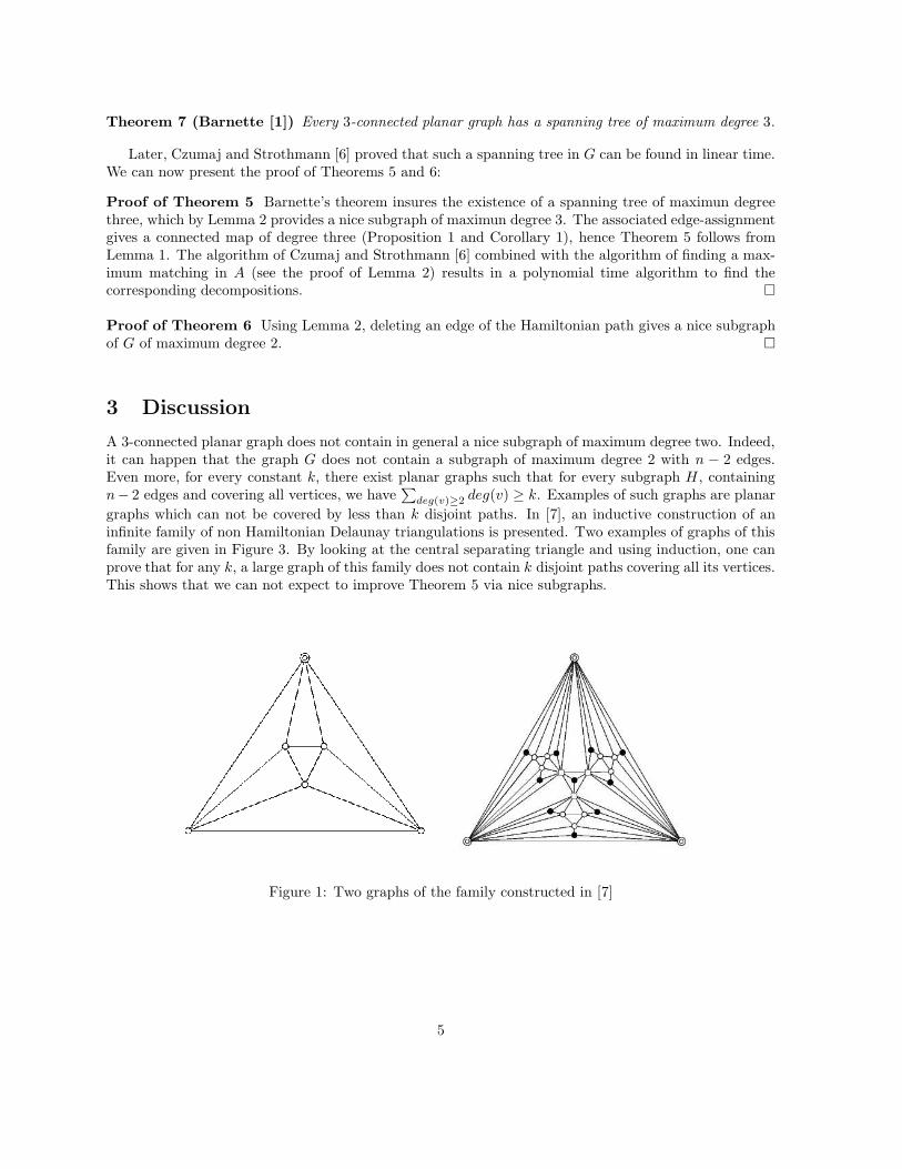
Theorem 7 (Barnette [1]) Every 3-connected planar graph has a spanning tree of maximum degree 3.
Later, Czumaj and Strothmann [6] proved that such a spanning tree in G can be found in linear time.We can now present the proof of Theorems 5 and 6:
Proof of Theorem 5 Barnette’s theorem insures the existence of a spanning tree of maximun degreethree, which by Lemma 2 provides a nice subgraph of maximun degree 3. The associated edge-assignmentgives a connected map of degree three (Proposition 1 and Corollary 1), hence Theorem 5 follows fromLemma 1. The algorithm of Czumaj and Strothmann [6] combined with the algorithm of finding a max-imum matching in A (see the proof of Lemma 2) results in a polynomial time algorithm to find thecorresponding decompositions.
Proof of Theorem 6 Using Lemma 2, deleting an edge of the Hamiltonian path gives a nice subgraphof G of maximum degree 2.
3 Discussion
A 3-connected planar graph does not contain in general a nice subgraph of maximum degree two. Indeed,it can happen that the graph G does not contain a subgraph of maximum degree 2 with n − 2 edges.Even more, for every constant k, there exist planar graphs such that for every subgraph H , containingn− 2 edges and covering all vertices, we have
∑deg(v)≥2 deg(v) ≥ k. Examples of such graphs are planar
graphs which can not be covered by less than k disjoint paths. In [7], an inductive construction of aninfinite family of non Hamiltonian Delaunay triangulations is presented. Two examples of graphs of thisfamily are given in Figure 3. By looking at the central separating triangle and using induction, one canprove that for any k, a large graph of this family does not contain k disjoint paths covering all its vertices.This shows that we can not expect to improve Theorem 5 via nice subgraphs.
Figure 1: Two graphs of the family constructed in [7]
5

Acknowledgements
The authors would like to thank David Coudert and Jean-Sebastien Sereni for interesting discussions.Special thanks to Frederic Havet and Stephan Thomasse for their comments on the first drafts of thispaper. We are also indebted to anonymous referees for valuable comments.
References
[1] D. Barnette. Trees in Polyhedral Graphs. Canadian Journal of Mathematics, (18):731–736, 1966.
[2] H. L. Bodlaender and F. V. Fomin. Approximation of Path-width of Outerplanar Graphs. Journalof Algorithms, 43(2):190–200, 2002.
[3] H.L. Bodlaender. Tree-width: Algorithmic Techniques and Results. Proceedings of 22nd Interna-tional Symposium MFCS, LNCS, 1295, 1997.
[4] V. Bouchitte, F. Mazoit, and I. Todinca. Chordal Embeddings of Planar Graphs. Discrete Mathe-matics, 273(1-3):85–102, 2003.
[5] D. Coudert, F. Huc, and J. S. Sereni. Path-width of Outerplanar Graphs. Journal of Graph Theory,55(1):27–41, 2007.
[6] A. Czumaj and W.B. Strothmann. Bounded Degree Spanning Trees. Algorithms, ESA 97 (Graz),Springer Lecture Notes in Computer Science 1284, pages 104–117, 1997.
[7] M. B. Dillencourt. Finding Hamiltonian Cycles in Delaunay Triangulations Is NP-Complete. DiscreteApplied Mathematics, 64(3):207–217, 1996.
[8] F. V. Fomin and D. M. Thilikos. On Self-Duality for Path-width in Polyhedral Graph Embeddings.Journal of Graph Theory, 55(1):42–45, 2007.
[9] D. Lapoire. Structuration des graphes planaires. PhD thesis, Universite de Bordeaux, France, 1999.
[10] B. Reed. Tree-width and tangles: an new connectivity measure and some applications. In R. A.Bayley, editor, Surveys in Combinatorics, pages 87–162. Cambridge University Press, 1997.
[11] N. Robertson and P. D. Seymour. Graph minors. I. Excluding a Forest. Journal of CombinatorialTheory Series B, 35(1):39–61, 1983.
[12] N. Robertson and P.D. Seymour. Graph minors. III. Planar tree-width. Journal of CombinatorialTheory Series B, 36(1):49–64, 1984.
[13] P. Seymour and R. Thomas. Call routing and the ratcatcher. Combinatorica, 14:217–241, 1994.
[14] T. Tutte. A Theorem on Planar Graphs. Transactions of American Mathematical Society, 82:99–116,1956.
6
314 Annexes
Annexe F
Mixing Digraphs
In this appendix I introduce a new parameter for digraphs called mixing. Adigraph D is said f -mixing if for every non necessarily disjoint pairs of subsetsA,B⊂V with e(A,B) ≥ f , we have e(B,A) > e(A,B). I then study the conditions onthis parameter which force a digraph D to contain a subdigraph H. In the case H =−→C4, I fully answer this question : there is some C1 < C2, such that every C1(e2/n2)-mixing digraph D contains a directed 4-cycle and such that, when e≥ 100n3/2,there is C2(e2/n2)-mixing digraph D without directed 4-cycles. I also answer thisquestion when H is non-bipartite and when D is dense. I finish this appendix onthe question of how mixing a digraph can be.
This appendix is based on a joint work with O. Amini and S. Griffiths. Part of theseresults have been presented at the conference LAGOS 07, which took place from the24th to the 28th of November 2007 in Chile.
Computing the best constants for the theorems we propose was not our objective,hence the constants given in the proofs are not the best possible.
Graphs and forbidden subgraphs. The idea underlying mixing digraphs is tofind a sufficient condition to force an oriented graph to have some specific patterns.Conversely we can see the problem as asking for the strongest conditions we can forcewhile avoiding those patterns. In our case, the pattern is given by a small digraph H,and given a digraph D, we say that either D has H as a subgraph or that D is H-free.More formally we can define subgraphs and H-free digraphs as follow :
Definition F.1 Given a digraph H on vertex set V(H) = u1, . . . ,uh and arc set E(H),we say that a digraph D contains H as a (non necessarily induced) subgraph iff thereis a set of h vertices of D, v1, . . . ,vh, such that for every arc uiu j of H, viv j is an arc ofD.
315

316 Annexes
We say a digraph D is H-free iff it does not contain H as a subgraph. Given a familyH , we say D is H -free if it is H-free for any H ∈H .
The analog problem has been studied for undirected graphs. Turan’s theorem ans-wers the question of the maximum number of edges a Kk-free graph can have, for all k.It says that it is (1−1/(k−1))n2/2,∀k∈ N∗. Given k∈ N, the extremal example is theTuran graph Tk−1 which has (1−1/(k−1))n2/2 edges and does not contain any graphof chromatic number k or more (and in particular they are Kk-free). A generalizationof this theorem due to P. Erdős and M. Simonovits in [ES66] states that these graphsare asymptotically extremal for every family H , each graph of which has chromaticnumber at least k and one of them has chromatic number exactly k. Denoting ex(n,H )the maximum number of edges a H -free graph on n vertices can have, one can statethis result as follows :
Theorem F.2 ([ES66]) Let H be a family, in which each graph has chromatic numberat least k and one of them has chromatic number exactly k, we have ex(n,H ) = (1−1/(k−1)+o(1))n2/2.
This theorem gives an asymptotic answer when k > 2, however, when k = 2, weonly get ex(n,H ) = o(n2). Still, more precise results are known, as for example whenH = C4, the 4-cycles : it was shown by P. Erdős, A. Rényi and V.T. Sós [ERS64]that ex(n,C4) = (1
2 + o(1))n3/2. In fact, for any n, they present a C4-free graph withedges which turns out to be extremal [Fur83]. Their example (which is produced usinga projective plane) is discussed further in Section F.1.2.
In 1973, in [BES73], W.G. Brown, P. Erdős and M. Simonovits studied the questionin the directed case. The digraphs they considered are without loops and multiplearcs, but they allow 2-cycles. Exactly, they considered the question of the maximumnumber of arcs a digraph on n vertices can have if it does not contain any digraphof a family H = H1, . . . ,Hq as subgraph. They proved the existence of a sequence ofasymptotically extremal graphs. Later, in [BES85], they proved it in an algorithmicway.
Theorem F.3 ([BES85]) There exist a finite algorithm which determines sequencesof digraphs which are asymptotically extremal for any given finite family H .
However, there is no simple characterization, similar to the minimal chromatic num-ber in simple graphs, of digraphs which arise in asymptotically extremal sequences.
When 2-cycles are forbidden. When H contains the directed 2-cycle−→C2, and
digraphs which are not acyclic, the transitive tournament D on vertex set V = 1, ...,n,and arc set E = i j : i < j is an extremal graph for H . Indeed D has
(n2
)
arcs (the mostpossible while avoiding 2-cycles) but contains no elements of H since it is acyclic. Soin this situation, no condition on the number of arcs guarantees the presence of H as asubgraph. However, in this example D has an extreme bias in its orientation : we can findsubsets A,B⊂V with e(A,B) = n2/4 but e(B,A) = 0. To obtain more information about
Annexes 317
the H -free digraphs when H contains the directed 2-cycle and non-acyclic digraphs, wepropose to investigate if only "strongly biased digraphs" can avoid containing elementsof H as subgraph.
Remark F.4 Given a set of forbidden digraphs H , if it contains the directed 2-cycle,investigating if only "strongly biased digraphs" can avoid containing elements of H assubgraph is equivalent to the same question over oriented graphs. Hence, from now on,instead of considering H with the directed 2-cycle, we will investigate the question onlyover oriented graphs.
When H contains a directed 4-cycle, we indeed prove that only "strongly biasedoriented graphs" can avoid containing elements of H . More precisely, we show that, iffor all subsets A,B⊂V with e(A,B)≥ e2/32n2 we have e(B,A) > e(A,B)/2, then D mustcontain a 4-cycle. This is Theorem F.10.
In Section F.2, we extend this result to dense oriented graphs when H is any setof digraphs, one of which is bipartite. However, when no element of H is bipartite, weprove that there are dense oriented graphs whose orientations are not biased and whichare H -free.
Mixing digraphs. To describe more precisely what we mean by "strongly biasedoriented graphs", we introduce a new notion : the notion of mixing digraphs.
Definition F.5 Given a digraph D, f ∈ R and γ ∈]0,1[ we say D is ( f ,γ)-mixing iffor every non necessarily disjoint pairs of subsets A,B ⊂ V with e(A,B) ≥ f , we havee(B,A) > γe(A,B). When γ = 1
2, we simply say f -mixing.
In other words, a digraph D is f -mixing if when we have a lot of arcs from a set Aof vertices to a set B (i.e. at least f arcs) then we have more than half as many back.More generally for γ ∈]0,1[ we say that D is ( f ,γ)-mixing if for every pair A,B⊂V withmore than f arcs from A to B, we have more than γe(A,B) arcs from B to A.
This definition gives us a large range of mixing conditions getting stronger as fdecreases. In particular e+1-mixing is a really weak condition as all digraphs are e+1-mixing. Hence the weakest mixing condition we will ask for will be when f = O(e).Being 1-mixing means that all arcs are in a 2-cycle. In the following, the conditionswe will use are mainly (in strengthening order when e is big enough) e-, (ek/n2)1/(k−1)-,e2/n2- and n-mixing.
Given this definition, one can ask for the weakest mixing condition which forcesan oriented graph to have a given digraph H as subgraph ? If we write mex(n,e,H) =minf ∀D, f −mixing, with e edges and n vertices: H ⊂ D the question is to determinemex(n,e,H). More generally we can ask, given a set H of forbidden subgraphs, formex(n,e,H ) = minf∀D f −mixing, with e edges and n vertices: ∃H ∈H : H ⊂ D
We fully answer this question when H is one of the orientation of the 4-cycle.
Definition F.6 We write−→C4 for the directed 4-cycle, a
−→C4 for the almost directed 4-
cycle, i.e., the oriented 4-cycle with a single reversed arc, p−→C4 for the 4-cycle made of

318 Annexes
≥ f edges
> f/2 edges
A
B
Fig. F.1 – Illustration of the mixing condition
s−→C4p
−→C4a
−→C4
−→C4
Fig. F.2 – The four different orientations of C4
two parallel paths of length two and s−→C4 for an antidirected 4-cycle, i.e., an oriented
4-cycle made of two 2-stars. This is illustrated by Figure F.2.
The main results of this section are Theorem F.10 and Corollary F.23 which give thevalue of mex(n,e,
−→C4) up to a multiplicative constant. There are some constants C1 < C2
such that :
C1e2
n2 ≤ mex(n,e,−→C4) ≤C2max(
e2
n2 ,n).
Before going any further, one has to insure that an f -mixing digraph indeed exists, atleast for some values of f . Thankfully this question is answered positively by Lemma F.7.In fact we prove much more : if G is a simple graph and D is obtained from G by orien-ting the arcs of G at random then D is Ln-mixing with positive and high probability(where L is a sufficiently large constant).
Lemma F.7 There exists L such that for any graph G on n vertices, the oriented graphD obtained by orienting the edges of G at random, is Ln-mixing with positive probability(always) and with high probability (as n tends to infinity). In particular, ∀ε > 0, if eis much larger than n3/2 then, for n large enough, Ln is less than εe2/n2 and so D is

Annexes 319
(εe2/n2)-mixing with positive probability and with high probability. More generally forany γ ∈]0,1[ there exists Lγ such that D is (Lγn,γ)-mixing with positive probability andwith high probability.
Proof.We prove the second, more general statement. For a pair (A,B)⊂V2 we write e(A,B)
for the number of arcs between A and B in the graph G. Consider a pair (A,B) ⊂ V2
with e(A,B)≥ Ln, L a constant to be defined later. From Chernoff’s inequality we have,
P(e(B,A) ≤ γe(A,B)) ≤ exp(−c(γ)e(A,B)) ≤ exp(−c(γ)Ln)
with c(γ) a positive constant dependent on γ. Set L = 2/c(γ). Let W = (A,B) : (A,B) ⊂V2ande(A,B)≥ Ln. Noting that there are only 4n ways to pick a pair of subsets (A,B)⊂V2 we have |W| ≤ 4n, and so
P(e(B,A) ≤ γe(A,B) for some pair (A,B) ⊂W) ≤ 4n exp(−c(γ)Ln) ≤ 4n exp(−2n).
This quantity goes to 0 as n tends to infinity. If an oriented graph G is not (Ln,γ)-mixing then there exist subsets (A,B) ⊂ V2 with e(A,B) ≥ Ln (implying (A,B) ⊂ W2)and e(B,A) < γe(A,B). So that with high probability D is (Ln,γ)-mixing.
Now that we know mixing digraphs exist, let us give some general results on mixingdigraphs.
Given a digraph D and a set of vertices A, we note by d+A (u) the number of arcs
from A to u and d−A (u) the number of arcs from u to A.
Lemma F.8 Let D be an f -mixing digraph and A a set of vertices. Most of the arcs areincidents to vertices u satisfying 1/2d+
A (u) ≤ d−A (u) ≤ 2d+
A (u), more precisely, at most3 f arcs do not have this property.
Proof. Set B = u,d+A (u) > 2d−
A (u). We have e(B,A) = ∑Bd+A (u) ≥ 2∑Bd−
A (u) = e(A,B),hence (A,B) does not satisfy the mixing condition and we have ∑Bd+
A (u) < f and∑Bd−
A (u) < f/2, hence at most 3/2 f arcs are incident to vertices with d+A (u) > 2d−
A (u).We proceed similarly for the other inequality.
Lemma F.9 Given an f -mixing digraph D and a set of vertices A⊂V, the number ofpaths of length two from A to A is at least (e(A,V)−3 f )2
2n .
Proof. The number of paths of length two from A to A is precisely ∑u∈Ad+A (u)d−
A (u).Set B = Γ+(A). Set W = u ∈ B : 1/2d+
A (u) ≤ d−A (u) ≤ 2d+
A (u). From Lemma F.8,we have e(A,W) ≥ e(A,V)−3 f . We can lower bound the number of path of length twofrom A to A by ∑Bd−
A (u)d+A (u) ≥ ∑W d−
A (u)d+A (u) ≥ 1/2∑Bd+
A (u)2 ≥ 1/2n(∑ d+A (u))2 ≥
1/2n(e(A,V)−3 f )2.

320 Annexes
F.1 On the value of mex(n,e,−→C )
In this section, we study mex(n,e,−→C ) when
−→C is a directed cycle of even length.
First we will give a lower bound for mex(n,e,−→C4), then we will give upper bounds for
mex(n,e,−→C4) and more generally for mex(n,e,
−→C2k) (under some assumptions). Finally we
will look at some lower bounds for mex(n,e,−→C2k).
F.1.1 A lower bound for mex(n,e,−→C4)
We now wish to show that if D obeys a certain mixing condition then it contains adirected 4-cycle. (We do not require any separate condition on e, but we keep in mindthe case with e much larger than n3/2, a particular example being e= n1+α for someα ∈]0.5,1].) The main result of this section is, if C1 is small enough, every C1e2/n2-mixing oriented graph contains a directed 4-cycle. (For example when e = n1+α thecondition C1e2/n2-mixing, means C1n2α-mixing. For α ∈]0.5,1[ this is a strictly strongercondition than C1e-mixing and strictly weaker than C1n-mixing.)
Theorem F.10 For C1 = 1/32, every (C1e2/n2)-mixing oriented graph D contains adirected 4-cycle.
Remark F.11 i) In Section F.1.2, we give examples of oriented graph which are(C2e2/n2)-mixing (where C2 is a large constant) and do not contain directed4-cycles. This means that the mixing condition cannot be weakened, so Theo-rem F.10 is best possible.
ii) In the case where e is of order n2, it is not too difficult to deduce Theorem F.10using Szemerédi’s regularity Lemma (c.f. [KSSS02] for a survey and Section F.2).
In our proof we apply the mixing condition repeatedly, receiving on each applicationa new piece of information. We begin with Corollary F.12 that shows that there mustbe many paths of length 2. In fact this lemma requires only that D is e/6-mixing (thisis much weaker than our mixing condition because e/6 is much larger than e2/32n2)
For each v∈V, we write e(2)v for the number of paths of length two starting at v,
i.e., e(2)v = e(Γ+(v),Γ++(v)).
Corollary F.12 An e/6-mixing digraph D contains at least e2/8n paths of length two,i.e.,
∑v∈V
e(2)v ≥ e2/8n
Proof of Theorem F.10. This a direct consequence of Lemma F.9.
We now prove Theorem F.10 :Proof. We focus our attention on the set W = v∈V : e(2)
v ≥ e2/16n2.We let d+−(u,v) = |Γ+(u)∩Γ−(v)|, and similarly d++(u,v) = |Γ+(u)∩Γ+(v)|. These
joint degrees are useful for expressing quantities such as e(U,Γ+(v)) (for v∈V and U ⊂
On the value of mex(n,e,−→C ) 321
V), which can be expressed as e(U,Γ+(v)) = ∑u∈U d++(u,v). In particular we shall usethat, e(Γ++(v),Γ+(v)) = ∑u∈Γ++(v) d++(u,v) and e(Γ−−(u),Γ+(u)) = ∑v∈Γ−−(u) d++(u,v).
The idea is to note that for vertices v∈W, the quantity e(2)v = e(Γ+(v),Γ++(v)) is
quite large, so, by the mixing condition, e(Γ++(v),Γ+(v)) is also quite large. We thenchange perspective and view things from the point of view of vertices u∈ Γ++(v). Bydoing so we can prove that, using again the mixing conditions, there are arcs fromΓ+(u) to Γ−−(u).
Notice that even if we restrict ourselves to vertices in W, the number of paths oflength two starting at W is still large
∑v∈W
e(2)v ≥ ∑
v∈V
e(2)v − ∑
v∈V\We(2)
v ≥ e2/8n−ne2/16n2 ≥ e2/16n.
Now for each v ∈ W we have e(2)v = e(Γ+(v),Γ++(v)) ≥ e2/32n2. By the e2/32n2-
mixing condition, we have e(Γ++(v),Γ+(v)) ≥ e(2)v /2. In other words, for all v ∈ W,
∑u∈Γ++(v) d++(v,u) ≥ e(2)v /2.
Hence,
∑u
∑v∈Γ−−(u)
d++(v,u) = ∑v
∑u∈Γ++(v)
d++(v,u) ≥ 12 ∑
v∈W
e(2)v ≥ e2
32n.
So there exists u with ∑v∈Γ−−(u) d++(v,u) ≥ e2/32n2, i.e.,
e(Γ−−(u),Γ+(u)) ≥ e2/32n2.
By the mixing condition, we have e(Γ+(u),Γ−−(u)) ≥ e2/64n2. Since an arc fromΓ+(u) to Γ−−(u) gives an oriented 4-cycle and that e2/64n2 > 0 (as the empty graph isnot e2/32n2-mixing), we are done.
Interestingly, a variant of the above method allows us to find a large number of4-cycles rather than just one. In fact we shall show that, for some C′
1, in (C′1e2/n2)-
mixing oriented graph D, we can find ce4/n4 4-cycles (for some constant c > 0) whichis Theorem F.13. We shall prove this with c = 1/32768and C′
1 = 1/128 (which gives astronger mixing condition than the one which was used in the proof of Theorem F.10).
Theorem F.13 Every (e2/128n2)-mixing oriented graph D contains at least 1/32768e4/n4
directed 4-cycles.
There are two main weaknesses to the above count. Firstly we say that the numberof 4-cycles containing u is at least e(Γ+(u),Γ−−(u)). Whereas in fact each arc wv fromΓ+(u) to Γ−−(u) gives rise to not just one 4-cycle but d+−(v,u) 4-cycles. To take thisinto account we must restrict our attention to pairs v,u for which d+−(v,u) is not toosmall. The second main weakness is of course that we have been finding many 4-cyclescontaining a single vertex. For a better count we must consider a set of vertices U ⊂V,and find many 4-cycles for each u∈U .

322 Annexes
Recall that e(2)v = e(Γ+(v),Γ++(v)), and recall the set W = v∈V : e(2)
v ≥ e2/16n2.Observe that the set Γ++(v) is exactly u∈V : d+−(v,u)≥ 1. Our proof of Theorem F.10began by showing that for vertices v∈W there are many arcs from Γ+(v) to Γ++(v) andmany arcs back. We now wish to restrict our attention to pairs u,v for which d+−(v,u) isnot too small. So we define, for each v∈W, the set Tv = u∈Γ++(v) : d+−(v,u)≥ e(2)
v /2n.We are now ready to prove Theorem F.13.Proof of Theorem F.13. We have defined for each v∈W, a set Tv ⊂ Γ++(v), let usobserve that there are many arcs from Γ+(v) to Tv. By definition of Tv, e(Γ+(v),Γ++(v)\Tv) < e(2)
v /2, so that e(Γ+(v),Tv) ≥ e(2)v /2 ≥ e2/32n2. Now by the mixing condition,
e(Tv,Γ+(v)) ≥ e(Γ+(v),Tv)/2≥ e(2)v /4, for all v∈W. Using the joint degrees, we have
∑u∈Tv
d++(v,u) ≥ e(2)v
4for all v∈W.
It means that there are many arcs from Γ++(v) to Γ+(v). We now look from thepoint of view of vertices u in Γ++(v) which are destination of many paths of length two.Set Su = v∈W : u∈ Tv = v∈W : d+−(v,u) ≥ e(2)
v /2n, we have
∑u
∑v∈Su
d++(v,u) = ∑v∈W
∑u∈Tv
d++(v,u) ≥ 14 ∑
v∈W
e(2)v ≥ e2
64n.
We recall that e(Su,Γ+(u)) = ∑v∈Sud++(v,u), so that we have
∑u
e(Su,Γ+(u)) ≥ e2
64n.
Now consider the subset U ⊂ V defined by U = u ∈ V : e(Su,Γ+(u)) ≥ e2/128n2.It represents the vertices which have many out-neighbours which also are their in-in-neighbours, it gives many directed 4-cycles with an arc in the opposite direction. Wenote that the sum of e(Su,Γ+(u)) over vertices u∈V \U is at most e2/128n, and so,
∑u∈U
e(Su,Γ+(u)) ≥ e2
64n− e2
128n=
e2
128n.
As each vertex u∈U has e(Su,Γ+(u)) ≥ εe2/n2 we obtain from the mixing conditionthat e(Γ+(u),Su) ≥ e(Su,Γ+(u))/2 for each u∈U , and so
∑u∈U
e(Γ+(u),Su) ≥12 ∑
u∈U
e(Su,Γ+(u)) ≥ e2
256n.
This last equation means that there are many arcs which can replace the arc inthe opposite direction of the previously found almost directed 4-cycles. We count howmany directed 4-cycles it gives. For a vertex u∈ U an arc wv from Γ+(u) to Su givesrise to d+−(v,u) 4-cycles. Since v∈ Su ⊂W, we have that d+−(v,u) ≥ e(2)
v /2n≥ e2/32n3.For each u ∈ U let C4(u) be the number of 4-cycles with u in. We have that C4(u) ≥e(Γ+(u),Su)e2/32n3. Summing over vertices u∈U , we obtain
On the value of mex(n,e,−→C ) 323
∑u∈U
C4(u) ≥ e2
32n3 ∑u∈U
e(Γ+(u),Su) ≥e4
8192n4 .
Since each 4-cycle in D is counted at most four times by this sum we have found atleast e4/32768n4 4-cycles.
Remark F.14 The number of directed 4-cycles in a typical digraph (a graph in whicheverything is average) is of the order e4/n4. Hence the number of directed 4-cycles givento us by the above theorem is (up to multiplication by a constant) the largest we couldpossibly hope for. In fact any (e2/128n2)-mixing oriented graph contains thecorrect order of any orientation of a 4-cycle.
Theorem F.10 can be reformulated using the notation mex(n,e,−→C4) :
Corollary F.15 For n,e∈ N, we have
mex(n,e,−→C4) ≥
132
e2
n2 .
Notice that during the proof, we obtained the same result for almost directed 4-cycles a
−→C4, i.e., oriented 4-cycles with a reversed arc. Hence we have a similar theorem :
Theorem F.16 For n,e∈ N, we have
mex(n,e,a−→C4) ≥
132
e2
n2 .
Concerning 4-cycles consisting of two parallels paths of length two, p−→C4, it follows
from Lemma F.9 that the condition e/2 mixing is sufficient as soon as e≥ 2√
2n3/2. Thismixing condition is a lot weaker than the two previous ones but it needs a condition onthe number of arcs. Setting mexD:e≥m(n,e,H)= minf ∀D f-mixing, with n vertices and e edges, e≥m : H ⊂ D, we have :
Corollary F.17 For n,e∈ N, we have
mexD:e≥2√
2n2(n,e, p−→C4) ≥ e/2.
Concerning the last type of 4-cycles s−→C4, a condition on the number of arcs is
sufficient ; in fact almost the same condition as for 4-cycles in undirected graphs willbe sufficient.
Lemma F.18 The number of 2-stars (two arcs outgoing the same vertex) in a digraphis at least e2/n2.
This lemma is a direct application of Cauchy-Schwartz inequality. It then follows acorollary.
Corollary F.19 A digraph with more than n3/2 arcs contains a 4-cycle s−→C4 made of
two 2-stars.

324 Annexes
F.1.2 Upper bounds for some mex(n,e,−→C2k)
In the previous section we proved that every C1e2/n2-mixing oriented graph containsa 4-cycle (and in fact many). It is natural to ask whether this result would fail if C1
was replaced by a large constant C2. We give a class of examples of oriented graphswhich are C2e2/n2-mixing but which do not contain 4-cycles. Our class of examplesis comprehensive in the following sense : for a fixed large constant C2, and for anypair of natural numbers n and e, with e≥ 100n3/2, there is an oriented graph D withapproximately n vertices and approximately e arcs which is C2e2/n2-mixing but doesnot contain a directed 4-cycle.
F.1.3 Simple graphs with no 4-cycles
In constructing our examples we begin with a simple (undirected) graph G whichhas many edges but does not contain a 4-cycle. Let q be a prime power. The Erdős-Rényi graph G [ERS64] has V(G) being the set of points of the finite projective planePG(2,q) over the field of order q (so that n = q2 +q+1), and an edge between (x,y,z)and (x′,y′,z′) if and only if xx′ +yy′ +zz′ = 0. In fact this implies e(G) = 1
2q(q+1)2 andthis graph does not contain a 4-cycle. So for all n of the form q2 + q+ 1 (where q is aprime power) there is a graph G on n vertices with at least 1
2n3/2 edges which does notcontain a 4-cycle. We would like a result which holds for all n. We recall that Bertrand’spostulate states that for all k ≥ 2 there is a prime between k and 2k, combining thiswith the above example one may deduce that,
Lemma F.20 Given n≥ 2, there exists a (simple) graph G on n vertices with at least120n3/2 edges which does not contain a 4-cycle.
F.1.3.1 First examples
Let m∈N and let G be a 4-cycle free graph on m vertices with at least 120m3/2 edges.
For L the constant of Lemma F.7, by that lemma there exists an oriented graph Dobtained by orienting the edges of G which is Lm-mixing.
Setting n = m and e= e(D) = e(G), we have that D is our first example. For D isLm-mixing and since e2/n2 ≥ m3/400m2 = m/400 it follows that D is 400Le2/n2-mixing,and since G does not contain a 4-cycle, certainly D cannot contain any directed 4-cycle.
This example in itself does show that Theorem F.10 is best possible. It shows thatthe statement would fail if we set C1 = 400L. However this example itself does not showthat e2/n2 is the best expression we could have in the statement of the theorem. Toshow this we must give a class of examples of C2e2/n2-mixing oriented graphs which donot contain 4-cycles. These examples are obtained as blow ups of the first examples.
F.1.3.2 Blow-ups
An oriented graph D obeys a strong mixing condition, i.e., is f -mixing for a smallvalue of f , if it contains no large biased subgraphs. We show in this section that a
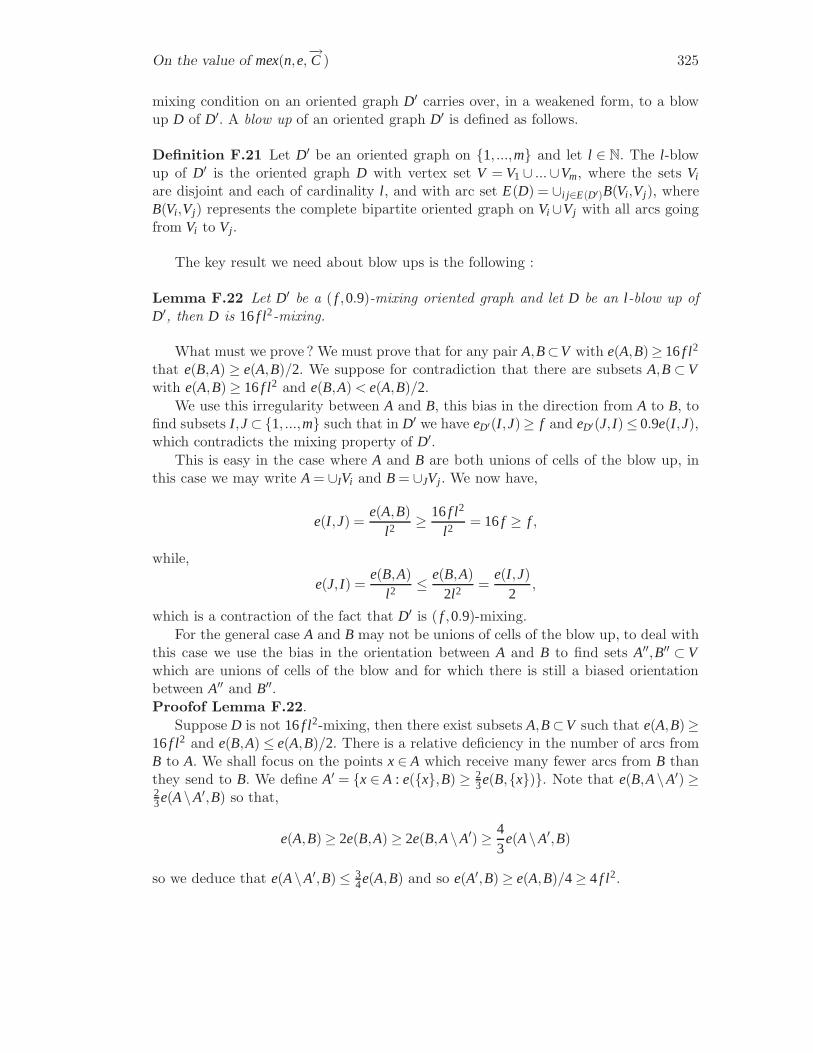
On the value of mex(n,e,−→C ) 325
mixing condition on an oriented graph D′ carries over, in a weakened form, to a blowup D of D′. A blow up of an oriented graph D′ is defined as follows.
Definition F.21 Let D′ be an oriented graph on 1, ...,m and let l ∈ N. The l -blowup of D′ is the oriented graph D with vertex set V = V1 ∪ ...∪Vm, where the sets Vi
are disjoint and each of cardinality l , and with arc set E(D) = ∪i j∈E(D′)B(Vi ,Vj), whereB(Vi ,Vj) represents the complete bipartite oriented graph on Vi ∪Vj with all arcs goingfrom Vi to Vj .
The key result we need about blow ups is the following :
Lemma F.22 Let D′ be a ( f ,0.9)-mixing oriented graph and let D be an l -blow up ofD′, then D is 16f l2-mixing.
What must we prove ? We must prove that for any pair A,B⊂V with e(A,B)≥ 16f l2
that e(B,A) ≥ e(A,B)/2. We suppose for contradiction that there are subsets A,B⊂Vwith e(A,B) ≥ 16f l2 and e(B,A) < e(A,B)/2.
We use this irregularity between A and B, this bias in the direction from A to B, tofind subsets I ,J⊂1, ...,m such that in D′ we have eD′(I ,J)≥ f and eD′(J, I)≤ 0.9e(I ,J),which contradicts the mixing property of D′.
This is easy in the case where A and B are both unions of cells of the blow up, inthis case we may write A = ∪IVi and B = ∪JVj . We now have,
e(I ,J) =e(A,B)
l2 ≥ 16f l2
l2 = 16f ≥ f ,
while,
e(J, I) =e(B,A)
l2 ≤ e(B,A)
2l2 =e(I ,J)
2,
which is a contraction of the fact that D′ is ( f ,0.9)-mixing.For the general case A and B may not be unions of cells of the blow up, to deal with
this case we use the bias in the orientation between A and B to find sets A′′,B′′ ⊂ Vwhich are unions of cells of the blow and for which there is still a biased orientationbetween A′′ and B′′.Proofof Lemma F.22.
Suppose D is not 16f l2-mixing, then there exist subsets A,B⊂V such that e(A,B)≥16f l2 and e(B,A) ≤ e(A,B)/2. There is a relative deficiency in the number of arcs fromB to A. We shall focus on the points x∈ A which receive many fewer arcs from B thanthey send to B. We define A′ = x∈ A : e(x,B) ≥ 2
3e(B,x). Note that e(B,A\A′) ≥23e(A\A′,B) so that,
e(A,B) ≥ 2e(B,A) ≥ 2e(B,A\A′) ≥ 43
e(A\A′,B)
so we deduce that e(A\A′,B) ≤ 34e(A,B) and so e(A′,B) ≥ e(A,B)/4≥ 4 f l2.

326 Annexes
For each x∈A′ we have e(x,B)≥ 23e(B,x). Let I = i :Vi ∩A′ 6= φ, now if i ∈ I then
there exists x∈A′∩Vi , now for any y∈Vi we know that y has exactly the same neighboursas x and so e(y,B) ≥ 2
3e(B,y). Defining A′′ = ∪IVi , we have e(A′′,B)≥ e(A′,B)≥ 4 f l2
and e(B,A′′) ≤ 23e(A′′,B).
We now begin a similar procedure to find B′′. Let B′ = y∈B : e(A′′,y)> 109 e(y,A′′),
this implies that e(B\B′,A′′) ≥ 910e(A′′,B\B′) so that,
e(A′′,B) ≥ 32
e(B,A′′) ≥ 32
e(B\B′,A′′) ≥ 2720
e(A′′,B\B′)
so we deduce that e(A′′,B\B′)≤ 2027e(A′′,B) and so e(A′′,B′)≥ 7
27e(A′′,B)≥ 14e(A′′,B)≥ f l2.
Let J = j : Vj ∩B′ 6= φ, and set B′′ = ∪JVj . With a similar argument to that givenpreviously we obtain that e(A′′,B′′) ≥ e(A′′,B′) ≥ f l2 and e(B′′,A′′) < 9
10e(A′′,B′′)This tells us that in D′ we have e(I ,J) ≥ f l2/l2 = f , while e(J, I) = e(B′′,A′′)/l2 <
9e(A′′,B′′)/10l2 = 9e(I ,J)/10. This contradicts the fact that D′ is ( f ,0.9)-mixing. Andso we have completed our proof that D is 16f l2-mixing.
F.1.3.3 The Class of examples
Let L equal the constant L0.9 of Lemma F.7 and let C2 = 6400L. Fix natural numbersm and l . Let G be a 4-cycle free graph on m vertices with at least m3/2/20 edges. ByLemma F.7 there exists an oriented graph D′ obtained by orienting the edges of G whichis (Lm,0.9)-mixing.
Properties of D’ :(i) |D′| = m,(ii) e(D′) ≥ m3/2/20,(iii) D′ is (Lm,0.9)-mixing,(iv) D′ does not contain a 4-cycle.
We now define D to be an l -blow up of D′, we note that D has the following pro-perties :
Properties of D :(i) |D| = ml,(ii) e(D) ≥ m3/2l2/20,(iii) D is 16Ll2m-mixing (for a proof, apply Lemma F.22),(iv) By inspection D does not contain a directed 4-cycle.
We also have
C2e(D)2
|D|2 ≥ C2(m3/2l2/20)2
(ml)2 =C2l2m400
= 16Ll2m,
so that D is C2e(D)2/|D|2-mixing.Hence for each m, l we obtain an oriented graph D which is C2e2/n2-mixing but
does not contain a 4-cycle. Furthermore this class of examples is general in the sensethat if we fix e0 and n0, with e0 ≥ 100n3/2
0 , then we may find an example D withapproximately e0 arcs and approximately n0 vertices with D being free of 4-cycles while

On the value of mex(n,e,−→C ) 327
being C2e2/n2-mixing, we may do this simply by choosing m to be an integer close ton4
0/400e20, choosing a 4-cycle free graph G with close to m3/2/20 edges and choosing l to
be close to 400e20/n3
0.
Corollary F.23 There exists some C2 such that, for n,e∈ N, we have
mex(n,e,−→C4) ≤C2max
(
e2
n2 ,n
)
.
Proof. When e > 100n3/2/20, the example described above are C2e2
n2 -mixing. Whene< 100n3/2, they are C2n-mixing.
It gives the same result for almost directed 4-cycles :
Corollary F.24 There exists some C2 such that, for n,e∈ N, we have
mex(n,e,a−→C4) ≤C2max
(
e2
n2 ,n
)
.
Considering now p−→C4, the previous example is of no interest. Indeed, as soon as we
do the blow up, there are plenty of p−→C4. However, the previous example is interesting
before the blow up since it shows that the condition on the number of arcs can notbe dropped. Indeed, the oriented graph D′, before the blow-up, is Ln-mixing (which isstrictly stronger than e/2-mixing), it has n vertices, 1
20n3/2 arcs and does not containany p
−→C4.
The following lemma gives upper bounds :
Lemma F.25 There exists a constant C′2 such that, for n,e∈ N, we have
when e≤ n2/2, mex(n,e,a−→C4) ≤ e+1,
when e≤ n3/2/20, mex(n,e,a−→C4) ≤C′
2n.
Proof. The only point which remains to prove is the first one.Consider the complete bipartite graph on vertex set V = V1∪V2 with V1 and V2 of
size n/2 and with all arcs going from V1 to V2. This oriented graph has no a−→C4. Finally
notice that all oriented graph are (e+1)-mixing.
At this point we have determined, up to a multiplicative constant, the value ofmex(n,e,H) when H is any orientation of C4. The next step is now to determine it whenH is a longer cycle. Notice that all cycles of odd length and more general orientationof non bipartite graphs will be treated in Section F.2.
F.1.4 Bounds for mex(n,e,−→C2k)
To find a lower bound for mex(n,e,−→C4), we strongly used the densest C4-free graph.
Hence to generalise this result we need dense C2k-free graphs.

328 Annexes
Hypothesis F.26 For k ∈ N , there exist C2k-free graphs on n vertices with cn1+1/k
edges for some constant c.
Due to a result of A. Bondy and M. Simonovits [BS74], this hypothesis is bestpossible. They prove the following theorem, which is usualy called the even circuittheorem :
Theorem F.27 ex(n,C2k) = O(n1+1/k)
But when do we know that this hypothesis really hold ?It was conjectured by P. Erdös and M. Simonovits [ES82] that ex(v,C2k)= 1/2v1+1/k+
o(v1+1/k).As mentioned before this conjecture is true for k = 2, it has also been proved in
[NV06] for k = 3 and disproved for k = 5 by a construction presented in [LUW95] evenif it is not mentioned in this paper. Still, for k = 5 our hypothsesis is valid for c≈ 0.58.For bigger values of k, less is known. The best lower bound is due to F. Lazebnik, V.A.Ustimenko and A.J. Woldar [LUW95] and is cn1+2/(3k), for some c.
We can notice that when all the graphs of even length less than 2k are forbidden,the previous lower bound is still valid and a better upper bound has been proved in[LV05], namely 1/2n1+1/k +2k2
n. This result is asymptotically tight for k∈ 2,3,5.Under Hypothesis F.26, Lemma F.22 implies :
Corollary F.28 Under Hypothesis F.26, let D′ be an (Lm,0.9)-mixing−→C2k-free oriented
graphs on m vertices with cn1+1/k edges and let l in N and let D be a blow up of D′ whereeach vertex is replaced by l vertices. There is a constant C independent of l such thatD is C(ek/n2)1/(k−1)-mixing.
From this lemma we can deduce an upper bound on mex(n,e,−→C2k).
Corollary F.29 Under Hypothesis F.26, there is some constant C2 such that mex(n,e,−→C2k)≤
C2max((ek/n2)1/(k−1),n).
It remains now to adapt Theorem F.13 to prove a lower bound. We do it for thedirected 6-cycle.
Theorem F.30 i) There exists C1 > 0 such that every (C1e2/n2)-mixing orientedgraph D contains a directed 6-cycle.
ii) There exists C′1 > 0 such that every (C′
1e2/ log(n)n2)-mixing oriented graph Dcontains at least ce6/n6 log(n) of them (for some constant c > 0).
Proof. We do not track the constant during the proof, instead we use a constant Cwhich evolves during the proof. We focus our attention on the set of vertices W′ = v∈V : d(v) ≥ e
16n (d(v) is the total degree, i.e., d+(v)+d−(v)) and on the set W = v∈W′ :
d(v) ≥ e16n and e(2)
v ≥ e2
16n2.
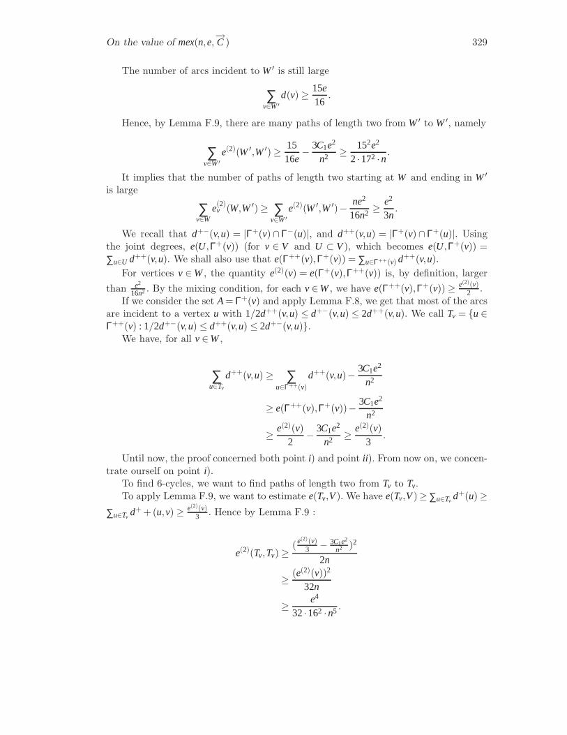
On the value of mex(n,e,−→C ) 329
The number of arcs incident to W′ is still large
∑v∈W′
d(v) ≥ 15e16
.
Hence, by Lemma F.9, there are many paths of length two from W′ to W′, namely
∑v∈W′
e(2)(W′,W′) ≥ 1516e
− 3C1e2
n2 ≥ 152e2
2·172 ·n.
It implies that the number of paths of length two starting at W and ending in W′
is large
∑v∈W
e(2)v (W,W′) ≥ ∑
v∈W′e(2)(W′,W′)− ne2
16n2 ≥ e2
3n.
We recall that d+−(v,u) = |Γ+(v)∩Γ−(u)|, and d++(v,u) = |Γ+(v)∩Γ+(u)|. Usingthe joint degrees, e(U,Γ+(v)) (for v ∈ V and U ⊂ V), which becomes e(U,Γ+(v)) =
∑u∈U d++(v,u). We shall also use that e(Γ++(v),Γ+(v)) = ∑u∈Γ++(v) d++(v,u).For vertices v ∈ W, the quantity e(2)(v) = e(Γ+(v),Γ++(v)) is, by definition, larger
than e2
16n2 . By the mixing condition, for each v∈W, we have e(Γ++(v),Γ+(v)) ≥ e(2)(v)2 .
If we consider the set A= Γ+(v) and apply Lemma F.8, we get that most of the arcsare incident to a vertex u with 1/2d++(v,u) ≤ d+−(v,u) ≤ 2d++(v,u). We call Tv = u∈Γ++(v) : 1/2d+−(v,u) ≤ d++(v,u) ≤ 2d+−(v,u).
We have, for all v∈W,
∑u∈Tv
d++(v,u) ≥ ∑u∈Γ++(v)
d++(v,u)− 3C1e2
n2
≥ e(Γ++(v),Γ+(v))− 3C1e2
n2
≥ e(2)(v)2
− 3C1e2
n2 ≥ e(2)(v)3
.
Until now, the proof concerned both point i) and point ii). From now on, we concen-trate ourself on point i).
To find 6-cycles, we want to find paths of length two from Tv to Tv.To apply Lemma F.9, we want to estimate e(Tv,V). We have e(Tv,V)≥ ∑u∈Tv
d+(u)≥∑u∈Tv
d+ +(u,v) ≥ e(2)(v)3 . Hence by Lemma F.9 :
e(2)(Tv,Tv) ≥(e(2)(v)
3 − 3C1e2
n2 )2
2n
≥ (e(2)(v))2
32n
≥ e4
32·162 ·n5 .
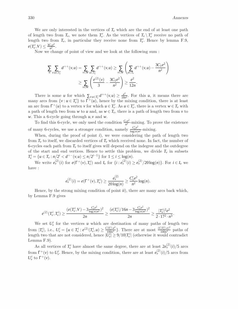
330 Annexes
We are only interested in the vertices of Tv which are the end of at least one pathof length two from Tv, we note them T ′
v . As the vertices of Tv \T ′v receive no path of
length two from Tv, in particular they receive none from T ′v . Hence by lemma F.9,
e(T ′v ,V) ≤ 3C1e2
n2 .Now we change of point of view and we look at the following sum :
∑u
∑v:u∈T ′
v
d++(v,u) = ∑v∈W
∑u∈T ′
v
d++(v,u) ≥ ∑v∈W
(
∑u∈Tv
d++(v,u)− 3C1e2
n2
)
≥ ∑v∈W
(
e(2)(v)3
− 3C1e2
n2
)
≥ e2
12n.
There is some u for which ∑v:u∈T ′vd++(v,u) ≥ e2
18n2 . For this u, it means there aremany arcs from v : u∈ T ′
v to Γ+(u), hence by the mixing condition, there is at leastan arc from Γ+(u) to a vertex v for which u∈ T ′
v. As u∈ T ′v , there is a vertex w∈ Tv with
a path of length two from w to u and, as w∈ Tv, there is a path of length two from v tow. This a 6-cycle going through u,v and w.
To find this 6-cycle, we only used the condition C1e2
n2 -mixing. To prove the existence
of many 6-cycles, we use a stronger condition, namely C′1e2
log(n)n2 -mixing.When, during the proof of point i), we were considering the path of length two
from Tv to itself, we discarded vertices of Tv which received none. In fact, the number of6-cycles each path from Tv to itself gives will depend on the indegree and the outdegreeof the start and end vertices. Hence to settle this problem, we divide Tv in subsetsT i
v = u∈ Tv : n/2i < d+−(v,u) ≤ n/2i−1 for 1≤ i ≤ log(n).We write e(2)
v (i) for e(Γ+(v),T iv) and Iv for i : e(2)
v (i) ≥ e(2)v /20log(n). For i ∈ Iv we
have :
e(2)v (i) = e(Γ+(v),T i
v) ≥e(2)
v
20log(n)≥ C′
1e2
n2 log(n).
Hence, by the strong mixing condition of point ii), there are many arcs back which,by Lemma F.9 gives
e(2)(T iv ,T
iv) ≥
(e(T iv ,V)−3 C′
1e2
log(n)n2 )2
2n≥
(e|T iv |/16n−3 C′
1e2
log(n)n2 )2
2n≥ |T i
v |2e2
2·172 ·n3 .
We set U iv for the vertices u which are destination of many paths of length two
from |T iv |, i.e., U i
v = u ∈ T iv : e(2)(T i
v ,u) ≥ C|T iv |·e2
100n3 . There are at most (C|T iv |·e)2
100n3 paths oflength two that are not considered, hence |U i
v| ≥ 9/10|T iv | (otherwise it would contradict
Lemma F.9).As all vertices of T i
v have almost the same degree, there are at least 2e(2)v (i)/5 arcs
from Γ+(v) to U iv. Hence, by the mixing condition, there are at least e(2)
v (i)/5 arcs fromU i
v to Γ+(v).

On the value of mex(n,e,H) in dense digraphs 331
Given i = 1, ..., l we write g(i) for the sum ∑v∈W ∑u∈U ivd++(v,u). We have
∑i
g(i) ≥∑i
15 ∑
v∈W
e(2)v (i) ≥ Ce2
n
and
∑i∈I
g(i) ≥ Ce2
2n.
Given i in I , ∑u∑v:u∈U ivd++(v,u) = ∑v∈W ∑u∈U i
vd++(v,u) = g(i) ≥ 10C′
1e2
nlog(n) . For each u
with ∑v:u∈U ivd++(v,u) at least C′
1e2
n2 log(n), we have many arcs from v : u ∈ U i
v to Γ+(u)
hence many arcs from Γ+(u) to v : u∈U iv.
Each arc gives many 6-cycles. Indeed, recall that u is the end of at least C|T iv |·e2
100n3
path of lengths two and for each of these paths, the starting vertex w has joint degreed+−(v,w) ≥ e(Γ+(v),T i
v)2|T i
v |≥ e2
(20·16·n2 log(n)).
Hence, each arc from Γ+(u) to v : u∈U iv gives at least Ce4
n5 log(n)6-cycles. The sum
(over u with ∑v:u∈U ivd++(v,u) at least C′
1e2
n2 log(n)) of the number of arcs Γ+(u) to v : u∈U i
vis at least Cg(i) which gives Ce4g(i)
n5 log(n)6-cycles. We can do the same thing for each i ∈ I
which in total gives Ce6
n6 log(n)6-cycles. Notice that we counted a 6-cycle at most six times.
Corollary F.31 There exist a constant C1 such that mex(n,e,−→C6) ≥ C1e2
n2 .
F.2 On the value of mex(n,e,H) in dense digraphs
In the previous section we gave results on the value of mexfor cycles of even length.We did it in a general setting and no assumptions on the underlying graph were taken.However, to consider more complicated types of patterns, i.e., more complicated digraphH ∈H , a possibility is to take more hypothesis on the underlying graph. In this sectionwe consider the case when the underlying graph issufficiently dense, i.e., it has morethan βn2 edges, for some β. Theorem F.33 says that the weakest mixing condition (linearin e) is sufficient to force such an oriented graph to have H as subgraph. However, whenH is non bipartite, it is essential to have D sufficiently dense. Indeed in PropositionF.32, we show that there exist digraphs with n2/4 edges satisfying the strongest mixingcondition we can hope for regular graph (linear in n) which contains no non bipartiteoriented graphs.
Proposition F.32 Let H be a non bipartite oriented graph on h vertices with chromaticindex k, for all n, for the constant L of Lemma F.7, there exist oriented graphs D with(1−1/(k−1))n2/2 arcs which are Ln-mixing and do not contain any copy of H.

332 Annexes
Proof. Just consider a the Turan’s graph Tk−1 oriented at random. Lemma F.7 says itis Ln-mixing for some constant L.
Theorem F.33 For every h, every oriented graph H on h vertices, for every γ ∈]0,1[,there exist ε > 0, 0 < β < 1
2, and an integer N such that every digraph D on n ≥ Nvertices, with βn2 arcs which is (εe,γ)-mixing contains H as a subgraph. When H isbipartite, β can be chosen if n is large enough.
Corollary F.34 Given an oriented graph H on h vertices, there exist ε > 0, 0< β < 12,
and an integer N such thatmexD:e≥βn2(n,e,H) ≥ εe.
Lemma F.35 Given an oriented graph H on h vertices which contains a directed pathof length two,
mexD:e≤n2/4(n,e,H) ≤ e+1.
Proof. This lemma is proved by the same oriented graph as the one which provedLemma F.25.
Consider the complete bipartite graph on vertex set V = V1∪V2 with V1 and V2 ofsize n/2 and with all arcs going from V1 to V2. This oriented graph is H-free and ise+1-mixing.
The proof of Theorem F.33 is based on the use of Szemerédi Lemma so we firststate it with the definitions we need.
Definition F.36 Let U and W be disjoint subsets of the vertices of some graph. Thenumber of edges between U and W (without taking into account orientation) is denotedby e(U,W). The density of the pair U,W is d(U,W) = e(U,W)
|U ||W| .
Definition F.37 Let 0 < σ < 1. The pair (U,W) is σ-uniform if, for all U ′ ⊂ U andW′ ⊂W with |U ′| > σ|U | and |W′| > σ|W| we have |d(U ′,W′)−d(U,W)| < σ.
A simple consequence of σ-uniformity is that the bipartite subgraph must be roughlyregular.
Lemma F.38 Let (U,W) be σ-uniform and let d(U,W) = d. Then |u∈U : |Γ(u)∩W|>(d−σ)|W|| ≥ (1−σ)|U | and |u∈U : |Γ(u)∩W| < (d+ σ)|W|| ≥ (1−σ)|U |
Definition F.39 An equipartition of V(G) into m parts is a partition V1, . . . ,Vm suchthat ⌊ n
m⌋ ≤ |Vi | ≤ ⌈ nm⌉, for 1 ≤ i ≤ m, where n = |V(G)|. The partition is σ-uniform if
(Vi ,Vj) is σ-uniform for all but σ(m
2
)
pairs 1≤ i < j ≤ m.
Lemma F.40 ([Sze75]) Let 0< σ < 1 and let l be a natural number. Then there existsL = L(l ,σ) such that every graph has a σ-uniform equipartition into m parts for somel ≤ m≤ L.

On the value of mex(n,e,H) in dense digraphs 333
Lemma F.41 Let H be an oriented graph on h vertices and γ ∈]0,1[. Let D a digraph,with e arcs, containing disjoint vertex sets V1, . . . ,Vh of size u or u+ 1 such that foreach (vi ,v j) ∈ E(H), (Vi ,Vj) is σ-uniform, d(Vi ,Vj) ≥ η and suppose that D(Vi ∪Vj) is(εe,γ)-mixing where ε = σ(η/(1+1/γ)−σ)
h2 . Furthermore we suppose (η/(1+1/γ))h ≥ (h+1)σ,σ/η ≤ 1 and σu≥ 1. Then D contains a subgraph isomorphic to H.
Proof. We call the vertices of H v1, . . . ,vh.We prove this statement by induction, we claim that the following property holds
for 0≤ l ≤ h :P (l) : x1, . . . ,xl can be chosen so that xi ∈Vi and, for l < j ≤ h there is a set Xl
j ⊂Vj
of candidates for x j at stage l , meaning that xiy j ∈ E(D) for every y j ∈ Xlj and every
xi ∈ N( j, l) = xi : 1≤ i ≤ l and viv j ∈ E(H). Moreover |Xlj | ≥ (η/(1+1/γ)−σ)N( j,l)u.
P (0) clearly holds, just take X0j = Vj .
Suppose P (l) true, we want to prove P (l +1).T+ represents the set of indices j, for which we have an outgoing arcs vl+1v j and so
we will have to be careful to have arcs from the vertex xl+1 we will select to the verticesof the set Xl+1
j . Yj is the set of vertices of Xll+1 which does not have enough arcs to Xl
jand hence that are not good candidates for xl+1.
For each t ∈ T+ = j > l +1 :vl+1v j ∈E(H), let Yt = y∈Xll+1 : |Γ+(y)∩Xl
t | ≤ (η/(1+1/γ)−σ)|Xl
t |.T− is the pendent of T+ for ingoing arcs.For each t ∈ T− = j > l +1 :v jvl+1 ∈E(H), let Yt = y∈Xl
l+1 : |Γ−(y)∩Xlt | ≤ (η/(1+
1/γ)−σ)|Xlt |.
By P (l) and the hypothesis, we have : |Xlt | ≥ (η/(1+1/γ)−σ)N( j,l)u≥ (η/(1+1/γ)−
σ)hu≥ σu.It follows from Definition F.37 and the (εe,γ)-mixing condition that for all t ∈
T+ ∪T−, |Yt | ≤ σu.Indeed, for t ∈ T+ :– if e(Yt ,Xl
t ) < εe, (η/(1+1/γ)−σ)|Xlt ||Yt | < εe so |Yt | < εe
(η/(1+1/γ)−σ)u ≤ σu.
– if e(Yt ,Xlt ) ≥ εe then by the mixing condition, e(Xl
t ,Yt) ≥ γe(Yt ,Xlt ). If e(Yt ,Xl
t ) ≥εe, then e(Yt ,Xl
t ) ≥ γe(Xlt ,Yt), and if e(Yt ,Xl
t ) ≤ εe, then e(Yt ,Xlt ) ≥ e(Xl
t ,Yt) whichalso gives e(Yt ,Xl
t ) ≥ γe(Xlt ,Yt). So e(Xl
t ,Yt) = e(Xlt ,Yt)+e(Xl
t ,Yt)≤ (1+1/γ)(η/(1+1/γ)−σ)|Xl
t ||Yt |, hence, d(Xlt ,Yt) ≤ (1+1/γ)(η/(1+1/γ)−σ) ≤ (η−σ) and so by
Definition F.37, |Yt | ≤ σu
We have the same result for t ∈ T−.Therefore |Xl
l+1\ (∪t∈T−∪T+Yt)| ≥ (η/(1+1/γ)−σ)N(l+1,l)u−|T−∪T+|σu≥ ((η/(1+
1/γ))N(l+1,l) −hσ)u≥ σu≥ 1. So we can select xl+1 ∈ Xll+1\ (∪t∈T−∪T+Yt).
It is now sufficient to take Xl+1t = Xl
t ∩Γ(xl+1) for t ∈ T− ∪T+ and Xl+1t = Xl
t fort /∈ T−∪T+ to obtain that P (l +1) is true.
The above shows that the claim holds for all l ,0≤ l ≤ h so x1, . . . ,xh can be foundas desired.
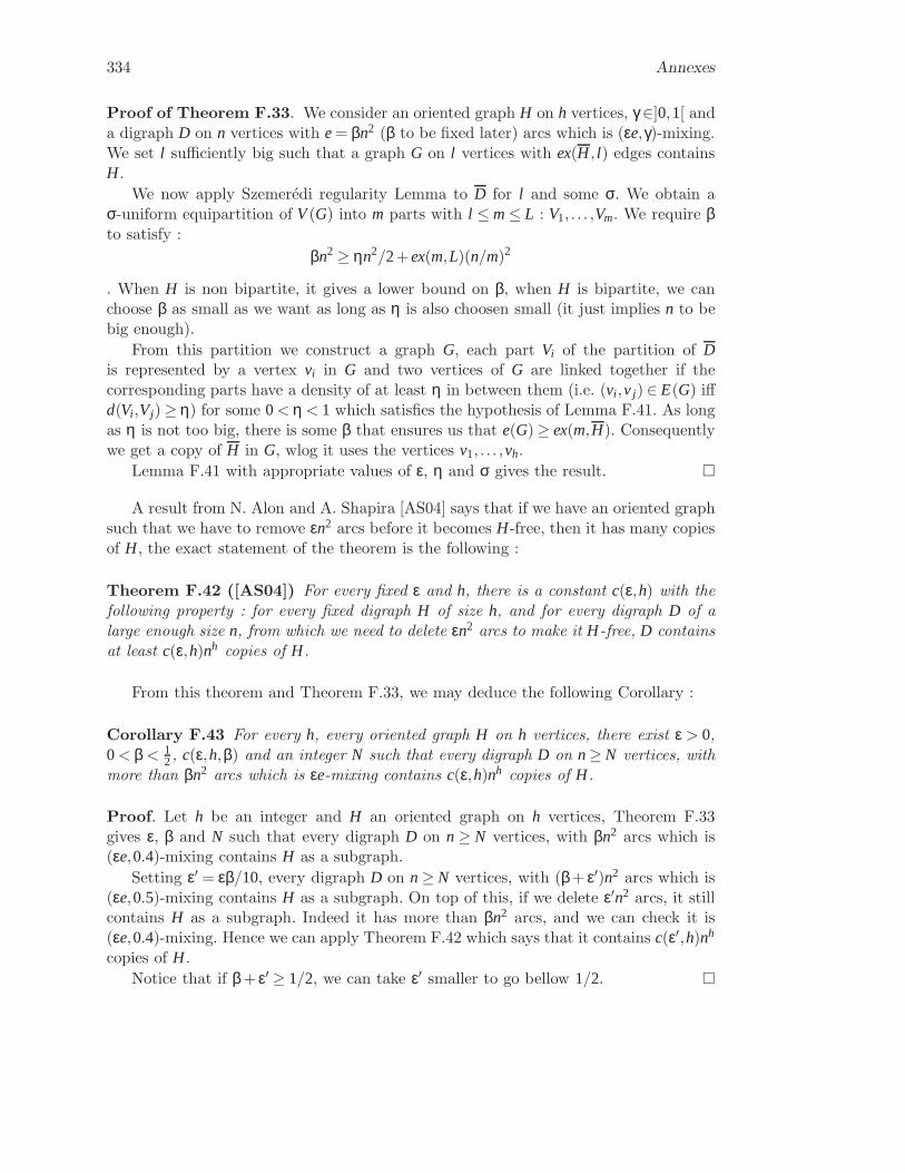
334 Annexes
Proof of Theorem F.33. We consider an oriented graph H on h vertices, γ ∈]0,1[ anda digraph D on n vertices with e= βn2 (β to be fixed later) arcs which is (εe,γ)-mixing.We set l sufficiently big such that a graph G on l vertices with ex(H , l) edges containsH.
We now apply Szemerédi regularity Lemma to D for l and some σ. We obtain aσ-uniform equipartition of V(G) into m parts with l ≤ m≤ L : V1, . . . ,Vm. We require βto satisfy :
βn2 ≥ ηn2/2+ex(m,L)(n/m)2
. When H is non bipartite, it gives a lower bound on β, when H is bipartite, we canchoose β as small as we want as long as η is also choosen small (it just implies n to bebig enough).
From this partition we construct a graph G, each part Vi of the partition of Dis represented by a vertex vi in G and two vertices of G are linked together if thecorresponding parts have a density of at least η in between them (i.e. (vi ,v j) ∈ E(G) iffd(Vi ,Vj) ≥ η) for some 0 < η < 1 which satisfies the hypothesis of Lemma F.41. As longas η is not too big, there is some β that ensures us that e(G) ≥ ex(m,H). Consequentlywe get a copy of H in G, wlog it uses the vertices v1, . . . ,vh.
Lemma F.41 with appropriate values of ε, η and σ gives the result.
A result from N. Alon and A. Shapira [AS04] says that if we have an oriented graphsuch that we have to remove εn2 arcs before it becomes H-free, then it has many copiesof H, the exact statement of the theorem is the following :
Theorem F.42 ([AS04]) For every fixed ε and h, there is a constant c(ε,h) with thefollowing property : for every fixed digraph H of size h, and for every digraph D of alarge enough size n, from which we need to delete εn2 arcs to make it H-free, D containsat least c(ε,h)nh copies of H.
From this theorem and Theorem F.33, we may deduce the following Corollary :
Corollary F.43 For every h, every oriented graph H on h vertices, there exist ε > 0,0 < β < 1
2, c(ε,h,β) and an integer N such that every digraph D on n≥ N vertices, withmore than βn2 arcs which is εe-mixing contains c(ε,h)nh copies of H.
Proof. Let h be an integer and H an oriented graph on h vertices, Theorem F.33gives ε, β and N such that every digraph D on n≥ N vertices, with βn2 arcs which is(εe,0.4)-mixing contains H as a subgraph.
Setting ε′ = εβ/10, every digraph D on n≥ N vertices, with (β+ ε′)n2 arcs which is(εe,0.5)-mixing contains H as a subgraph. On top of this, if we delete ε′n2 arcs, it stillcontains H as a subgraph. Indeed it has more than βn2 arcs, and we can check it is(εe,0.4)-mixing. Hence we can apply Theorem F.42 which says that it contains c(ε′,h)nh
copies of H.Notice that if β+ ε′ ≥ 1/2, we can take ε′ smaller to go bellow 1/2.

maxABD 335
This corollary says that given h, there exist ε > 0, 0< β < 12, c(ε,h,β) and an integer
N such that every digraph D on n≥N vertices, with βn2 arcs which is εe-mixing containsthe correct order of any orientation of any graph on h vertices.
F.3 maxABD
Lemma F.7 says that, if C is a large constant, randomly oriented graphs are Cn-mixing with high probability. It is now natural to wonder what is the strongest mixingcondition we can ask for. In general it seems really hard to determine how much anoriented graph is mixing, however, the presence of sets of vertices A and B with arcsfrom A to B and none from B to A (e(A,B) > 0 and e(B,A) = 0) is a natural obstructionfor an oriented graph to be highly mixing and is simpler to analyse. We define moreprecisely this problem in next section together with a complexity result. In SectionF.3.2 we give lower bounds for this number of arcs.
F.3.1 Definition and complexity result
To better understand how mixing we can ask for a digraph to be, we ask the followinggeneral question :
Given an oriented graph D, what is the maximum of arcs we can have from a set toan other with no arcs backward, i.e., what is :
ABmax
D= max
A,B:e(B,A)=0(e(A,B))?
In fact this question can be asked for digraphs in general and not only for orientedgraphs, i.e., we can ask this question when multiple arcs and 2-cycles are allowed. Inthis case, we have the following complexity result :
Theorem F.44 Given a digraph, potentially with 2-cycles, computing maxABD is NP-
hard and hard to approximate within a factor n1/2−ε for any ε > 0 unless P = NP.
Proof. We prove this theorem by reducing the stable set problem to our problem. Recallthat the stable set problem consists in finding a set as large as possible of independentvertices in a graph.
Given a graph G = (V,E), we construct a bipartite digraph as follow :– It has vertex set V1×V2 = V ×V.– Given an arc vw of G, we put a 2-circuit between the two vertices v ∈ V1 and
w∈V2.– Given v∈V, we put an arc from v∈V1 to v∈V2.It is now easy to see that a solution to maxAB
D , i.e., two sets A and B with e(A,B) =maxAB
D and e(B,A) = 0, gives a solution to the stable set problem. Indeed each arc fromA to B corresponds to a vertex and all the corresponding vertices form a stable set sinceotherwise there would be a 2-circuit with one end vertex in A and the other one in B.This stable set has to be maximal otherwise we could increase maxAB
D .

336 Annexes
It follows from a result of J. Håstad in [Hås99] that maxABD is NP-hard and hard to
approximate within a factor n1/2−ε for any ε > 0 unless P = NP.
F.3.2 Lower bounds on maxABD
In a digraph, maxABD can be equal to zero if all arcs are included in a 2-cycle, but
this is strongly due to the presence of 2-cycles. What happens when the digraph has no2-cycles ? We prove that for d-regular oriented graphs (oriented graph such that forall vertices v∈V we have d−(v) = d+(v) = d), maxAB
D is at least linear in n. In particular,this means that d-regular oriented graphs cannot be εn-mixing for small ε. To prove it,we construct two sets A and B with many arcs from A to B and none from B to A. Wedo this using a greedy algorithm.
In fact we just need to construct A since B can be chosen to maximize e(A,B) whilekeeping e(B,A) = 0, i.e., given A, we take B(A) = v : e(v,A) = 0.
1: Let v∈V, set A = v and B = Γ+(v).2: For all u∈V \A evaluate the function :
f (u) = ∑v∈A
(
1uv∈E +1vu∈E + |Γ+(v)∩Γ−(u)|+ |Γ+(u)∩Γ−(v)|)
.
3: while there is a vertex u with f (u) < d+(u) do4: Add to A the vertex v which maximizes d+(v)− f (v).5: Update B : B = B(A).6: Update f (u) for all u∈V \A.7: end while8: return A and B.
Using this algorithm on d-regular oriented graphs, one can prove :
Lemma F.45 Let D be a d-regular oriented graph, we can construct subsets A,B⊂Vwith e(A,B) ≥ n(d+1)
4d+6 − d− 1 and e(B,A) = 0 in polynomial time. In particular D is
emphatically not n(d+1)4d+6 −d−1-mixing.
Proof. Using the previous algorithm, we define a sequence of pairs of subsets At ,Bt ⊂V,with the property that e(Bt ,At) = 0 for all t. We attempt to do this while increasing thevalue of e(At ,Bt) so that for some value of t we have e(At ,Bt) ≥ n(d+1)
4d+6 −d−1.At is defined inductively adding one vertex at each step so that |At | = t.First choose any x1 ∈V, set A1 = x1 and B1 = B(A1).We now look for a suitable candidate y to join At = x1, ...,xt, it is unhelpful if y is
joined to A (in either direction) or if there are many paths of length two between them(in either direction). It is why we define the function ft : V \At → N by
ft(y) =t
∑i=1
(
1yxi∈E +1xiy∈E + |Γ+(xi)∩Γ−(y)|+ |Γ+(y)∩Γ−(xi)|)
.

maxABD 337
Counting arcs involving At and using regularity we have that, ∑y6∈Atft(y) ≤ t(2d2 +2d),
so that there exists y with ft(y) ≤⌊
2td(d+1)n−t
⌋
. Hence the xt+1 chosen by the algorithm is
such that ft(xt+1) ≤⌊
2td(d+1)n−t
⌋
. We now let At+1 = x1, ...,xt+1 and Bt+1 = B(At+1)
We wish to calculate e(At+1,Bt+1).It is clear that by adding xt+1 to At , we add d outgoing arcs but some of the added
arcs do not count, how many ? Precisely ∑ti=1
(
1xt+1xi∈E + |Γ+(xt+1)∩Γ−(xi))
.
Furthermore, we have Bt+1 ⊂ Bt , hence some arcs that we were counting beforedo not count anymore, how many arcs do we have to remove ? There are exactly
∑ti=1
(
1xixt+1∈E + |Γ+(xi)∩ Γ−(xt+1)|))
arcs we were counting before that we can notcount anymore.
In total it gives e(At+1,Bt+1) = e(At ,Bt)+d− ft(xt+1)≥ e(At ,Bt)+d−⌊
2td(d+1)n−t
⌋
and of
course e(Bt+1,At+1) = 0. It is now trivial by induction that e(At ,Bt)≥ td−∑ti=0
⌊
2id(d+1)n−i
⌋
for all t ≤ n2d+3. The algorithm goes until at least t =
⌊
n2d+3
⌋
and we have :
e(At ,Bt) ≥ td−⌊ n
2d+3⌋∑i=0
⌊
2id(d+1)
n− i
⌋
(F.1)
≥ td−d−1
∑i=0
i ∗ (
⌈
(i +1)n2d(d+1)+ i +1
⌉
−⌈
in2d(d+1)+ i
⌉
)
= td−⌈
d(d−1)n2d(d+1)+d
⌉
+d−1
∑1
⌈
in2d(d+1)+ i
⌉
≥ nd2d+3
−d−⌈
d(d−1)n2d(d+1)+d
⌉
+nd(d−1)
2(2d(d +1)+d−1)
≥ nd2d+3
−d− (d−1)n2d+3
−1+n(d−1)
2(2d+3)
≥ nd2d+3
− n(d−1)
4d+6−d−1
≥ n(d+1)
4d+6−d−1
And as we have already mentioned, by the choice of Bt , e(Bt ,At) = 0.
This result shows that there exist two sets A and B with many arcs from A to B andnone in the other direction. Furthermore it gives a way to construct this two sets. Ifwe are not interested in finding the sets A and B, we can use a probabilistic argumentwhich gives a slightly better result :
Lemma F.46 Let D be a d-regular oriented graph, there exist subsets A,B ⊂ V withe(A,B) ≥ n
4 and e(B,A) = 0. So that D is emphatically not n4-mixing.
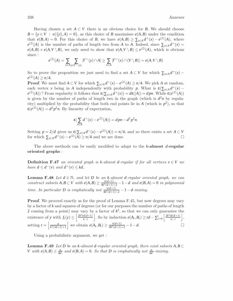
338 Annexes
Having chosen a set A ⊂ V there is an obvious choice for B. We should chooseB = y∈V : e(y,A) = 0, as this choice of B maximises e(A,B) under the conditionthat e(B,A) = 0. For this choice of B, we have e(A,B) ≥ ∑x∈A d+(x)− e(2)(A), wheree(2)(A) is the number of paths of length two from A to A. Indeed, since ∑x∈Ad+(x) =e(A,B)+ e(A,V \B), we only need to show that e(A,V \B) ≤ e(2)(A), which is obvioussince :
e(2)(A) = ∑x∈A
∑y∈Γ+(x)
|Γ+(y)∩A| ≥ ∑x∈A
|Γ+(x)∩ (V \B)| = e(A,V \B)
So to prove the proposition we just need to find a set A ⊂ V for which ∑x∈Ad+(x)−e(2)(A) ≥ n/4.Proof. We must find A⊂V for which ∑x∈A d+(x)−e(2)(A)≥ n/4. We pick A at random,each vertex v being in A independently with probability p. What is ε(∑x∈A d+(x)−e(2)(A)) ? From regularity it follows that ε(∑x∈A d+(x)) = dε(|A|) = dpn. While ε(e(2)(A))is given by the number of paths of length two in the graph (which is d2n by regula-rity) multiplied by the probability that both end points lie in A (which is p2), so thatε(e(2)(A)) = d2p2n. By linearity of expectation,
ε(∑x∈A
d+(x)−e(2)(A)) = dpn−d2p2n.
Setting p = 2/d gives us ε(∑x∈A d+(x)−e(2)(A)) = n/4, and so there exists a set A⊂Vfor which ∑x∈A d+(x)−e(2)(A) ≥ n/4 and we are done.
The above methods can be easily modified to adapt to the k-almost d-regularoriented graphs :
Definition F.47 an oriented graph is k-almost d-regular if for all vertices v ∈ V wehave d ≤ d−(v) and d+(v) ≤ kd,
Lemma F.48 Let d ∈ N, and let D be an k-almost d-regular oriented graph, we canconstruct subsets A,B⊂V with e(A,B)≥ n(d+1)
4k2(d+1)+2 −1−d and e(B,A) = 0 in polynomial
time. In particular D is emphatically not n(d+1)4k2(d+1)+2 −1−d-mixing.
Proof. We proceed exactly as for the proof of Lemma F.45, but now degrees may varyby a factor of k and squares of degrees (or for our purposes the number of paths of length2 coming from a point) may vary by a factor of k2, so that we can only guarantee theexistence of y with ft(y) ≤
⌊
2k2td(d+1)n−t
⌋
. So by induction e(At ,Bt) ≥ td−∑ti=0
⌊
2k2id(d+1)n−i
⌋
,
setting t =⌊
nk2(2d+2)+1
⌋
we obtain e(At ,Bt) ≥ n(d+1)4k2(d+1)+2 −1−d.
Using a probabilistic argument, we get :
Lemma F.49 Let D be an k-almost d-regular oriented graph, there exist subsets A,B⊂V with e(A,B) ≥ n
4k2 and e(B,A) = 0. So that D is emphatically not n4k2 -mixing.

Conclusion and Remaining questions 339
Now we note that if we randomly orient a random graph then with high probabilityit will be 2-almost d-regular for some d. Hence we may deduce :
Corollary F.50 Let G be a random graph on n vertices with each edge included inde-pendently with probability p (this is usual denoted G(n, p)) and let D be obtained fromG by orienting its edges at random. If p = ω(logn/n) then w.h.p. there exist subsets(A,B) ⊂V(G)2 with e(A,B) ≥ n
16 and e(B,A) = 0. So that w.h.p. D is emphatically notn16-mixing when n is large.
Proof. Two applications of the Chernoff inequality show that with high probability allthe degrees (out-degrees and in-degrees) are between 0.7pn and 1.4pn and so we aredone by applying Lemma 4.2 with d = 0.7pn.
This results have been completed by S. Griffiths in [Gri07], in which he proves that ifan oriented graph D has no isolated vertices then maxAB
D ≥ n/8log(n) and that this resultis best possible up to a constant factor by producing an example of a random orientedgraph which with high probability has no isolated vertices and for which maxAB ≤Cn/ log(n) for C a large constant.
F.4 Conclusion and Remaining questions
There are many questions one could ask concerning mixing properties. The mostimmediate is to ask what are the exact results for cycles other than 4-cycles. Perhapsthe most interesting case to consider next is the oriented 6-cycle. Theorem F.30 inwhich we show that there is a constant ε > 0 for which every εe2/n2-mixing orientedgraph contains a 6-cycle may not be the best possible. The upper bound we gave formex(n,e
−→C6) is Ce3/2/n for a large constant C. We believe that this is close to being best
possible. Specifically we conjecture,
Conjecture F.51 For, n and e, there exists ε > 0, such that every εe3/2/n-mixingoriented graph on n vertices and e edges, contains a directed 6-cycle. When e>> n4/3,it would imply mex(n,e
−→C6) = Ω(e3/2/n).
Similar conjectures can be made for even cycles of length 2k greater than 6, theywould simply say that the example obtained by taking a blow up of a random orientationof the largest graph of girth greater than 2k is (up to multiplication by constant) themost mixing oriented graph which does not contain a 2k-cycle.
More generally for a fixed oriented graph F, what mixing condition is required toensure D contains a copy of F ? This question has been answered when the underlyinggraph is dense, but what happen if it is not dense ? What can we say about anyorientation of a tree, is there some class of oriented graph for which it is easy to answerthis question ?

340 Annexes

Bibliographie
Ch. 2 : Notions de base
[CLR05] M.C. Costa, L. Létocart, and F. Roupin. Minimal multicut and maximal inte-ger multiflow : A survey. European Journal of Operational Research, 162(1) :55–69,2005.
[CR02] D. Coudert and H. Rivano. Lightpath assignment for multifibers wdm net-works with wavelength translators. In Global Telecommunications Conference,2002. GLOBECOM ’02. IEEE, volume 3, pages 2686–2690vol.3, 17-21 Nov. 2002.OPNT-01-5.
[CRR03] D. Coudert, H. Rivano, and X. Roche. A combinatorial approximation al-gorithm for the multicommodity flow problem. In K. Jansen and R. Solis-Oba,editors, WAOA 03, number 2909 in Lecture Notes in Computer Science, pages256–259, Budapest, Hungary, September 2003. Springer-Verlag.
[DDS05] G. Desaulniers, J. Desrosiers, and M.M. Solomon. Column Generation. Klu-wer Academic Publishers, Boston, MA, 2005.
[Fle00] L.K. Fleischer. Approximating Fractional Multicommodity Flow Independentof the Number of Commodities. SIAM Journal on Discrete Mathematics,13(4) :505–520, 2000.
[GVY93] N. Garg, V.V. Vazirani, and M. Yannakakis. Approximate max-flow min-(multi)cut theorems and their applications. In ACM Symposium on Theory ofComputing, pages 698–707, 1993.
[JMT05] B. Jaumard, C. Meyer, and B. Thiongane. On Column Generation Formu-lations for the RWA Problem. International Network Optimization Conference(INOC’O5), Lisbon, Portugal, pages 20–23, March 2005.
[Rag88] P. Raghavan. Probabilistic construction of deterministic algorithms : approxi-mating packing integer programs. Journal of Computer and System Sciences,37(2) :130–143, 1988.
341

342 Bibliographie
Ch. 3 : Conception de réseaux tolérants aux pannes
[ABG+06] O. Amini, J.-C. Bermond, F. Giroire, F. Huc, and S. Pérennes. Design of mi-nimal fault tolerant networks : Asymptotic bounds. In Huitièmes Rencontres Fran-cophones sur les Aspects Algorithmiques des Télécommunications (AlgoTel’06),pages 37–40, Trégastel, France, May 2006.
[AC03] N. Alon and M. Capalbo. Smaller explicit superconcentrators. Proceedings ofthe Fourteenth Annual Symposium on Discret Algorithms ACM-SIAM (SODA),pages 340–346, 2003.
[AGHP] O. Amini, F. Giroire, F. Huc, and S. Pérennes. Minimal selectors and faulttolerant networks. Networks. To appear.
[AGM87] N. Alon, Z. Galil, and V.D. Milman. Better expanders and superconcentra-tors. Journal of Algorithms, 8 :337–347, 1987.
[AHK99] N. Alon, P. Hamburger, and A.V. Kostochka. Regular honest graphs, isope-rimetric numbers, and bisection of weighted graphs. European Journal of Combi-natorics, 1999.
[AHU74] A.V. Aho, J.E. Hopcroft, and J.D. Ullman. The Design and Analysis ofComputer Algorithms. Addison-Wesley Longman Publishing Co., Inc., Boston,MA, USA, 1974.
[Alo86] N. Alon. Eigenvalues and expanders. Combinatorica, 6(2) :83–96, 1986.[Alo93] N. Alon. On the edge-expansion of graphs. Combinatorics, Probability and
Computing, 11 :1–10, 1993.
[AM84] N. Alon and V.D. Milman. Eigenvalues, expanders and superconcentra-tors. Proceedings of 25th Annual Symposium on Fondations of Computer Science(FOCS), pages 320–322, October 1984.
[BDD02] J-C. Bermond, E. Darrot, and O. Delmas. Design of fault tolerant on-boardnetworks in satellites. Networks, 40 :202–207, 2002.
[BGP07] J-C. Bermond, F. Giroire, and S. Pérennes. Design of Minimal Fault TolerantOn-Board Networks : Practical constructions. In 14th International Colloquium onStructural Information and Communication Complexity (SIROCCO 07), volume4474 of Lecture Notes in Computer Sciences, pages 261–273, Castiglioncello, Italy,June 2007.
[BHT06] J-C. Bermond, F. Havet, and D. Tóth. Fault tolerant on board networks withpriorities. Networks, 47(1) :9–25, 2006.
[BL06] Y. Bilu and N. Linial. Lifts, discrepancy and nearly optimal spectral gaps.Combinatorica, 26(5) :495–519, 2006.
[Bol88] B. Bollobás. The isoperimetric number of random regular graphs. EuropeanJournal of Combinatorics, 9(3) :241–244, 1988.
[Chu97] F.R.K. Chung. Spectral graph theory Regional conference series in mathema-tics, volume 92. American Mathematical Society, 1997.
Bibliographie 343
[CRVW02] M. Capalbo, O. Reingold, S. Vadhan, and A. Wigderson. Randomnessconductors and constant-degree lossless expanders. In 34th ACM Symposium onTheory of Computing (STOCS), pages 659–668, 2002.
[Dar97] E. Darrot. Diffusion de messages longs et propriétés structurelles dans lesréseaux d’interconnexion. PhD thesis, École doctorale STIC, Université de Nice-Sophia Antipolis, June 1997.
[DHMP06] O. Delmas, F. Havet, M. Montassier, and S. Pérennes. Design of faulttolerant on-board networks. Research report, INRIA Research Report 5866, March2006.
[DN01] D-Z. Du and H.Q. Ngo. Notes on the complexity of switching networks, pages307–367. Kluwer Academic Publishers, Dordrecht, The Netherlands, 2001.
[DSV03] G. Davidovf, P. Sarnak, and A. Valette. Elementary Number Theory, GroupTheory, and Ramanujan Graphs. Cambridge University Press, 2003.
[EH78] K.Y. Eng and M. Hecht. Switch matrix for TWTA redundancy on communica-tion satellites. National Telecommunications Conference (NTC’78), 3, December1978.
[Gir06] F. Giroire. Réseaux, algorithmique et analyse combinatoire de grands ensembles.PhD thesis, Université Paris 6, France, November 2006.
[Hav06] F. Havet. Repartitors, selectors and superselectors. Journal of InterconnexionNetworks, 7(3) :391–415, 2006.
[LV83] G. Lev and L.G. Valiant. Size bounds for superconcentrators. Journal of Theo-retical Computeur Science, 22 :233–251, 1983.
[Mor94] M. Morgenstern. Existence and Explicit Constructions of q+1 regular Rama-nujan Graphs for Every Prime Power q. Journal of Combinatorial Theory SeriesB, 62 :44–62, 1994.
[MP06] B. Monien and R. Preis. Upper bounds on the bisection width of 3-and 4-regular graphs. Journal of Discrete Algorithms, 4(3) :475–498, 2006.
[Pin73] M. Pinsker. On the complexity of a concentrator. 7th International TeletrafficConference, 318, 1973.
[Pip77] N. Pippenger. Superconcentrators. SIAM Journal on Computing, 6 :298–304,1977.
[RVW02] O. Reingold, S. Vadhan, and A. Wigderson. Entropy waves, the zig-zaggraph product, and new constant-degree expanders and extractors. Annals ofMathematics, 155(1) :157–187, 2002.
[Sch06] U. Schöning. Smaller superconcentrators of density 28. Information ProcessingLetters 98, 4 :127–129, 2006.
[Val75] L.G. Valiant. On non-linear lower bounds in computational complexity. In Pro-ceedings of seventh annual ACM symposium on Theory of computing (STOC’75),pages 45–53, New York, NY, USA, 1975. ACM.
344 Bibliographie
Ch. 4 : Algorithmes de routage
[AAG+05] S. Alouf, E. Altman, J. Galtier, J.F. Lalande, and C. Touati. An algorithmfor satellite bandwidth allocation. In Proceedings of IEEE infocom 2005, volume 1,pages 560–571, 2005.
[AAG+06] S. Alouf, E. Altman, J. Galtier, J.F. Lalande, and C. Touati. Quasi-OptimalResource Allocation in Multi-Spot MFTDMA Satellite Networks. CombinatorialOptimization in Communication Networks, 2006.
[AHSZ08] O. Amini, F. Huc, I. Sau Valls, and J. Zerovnik. (ℓ,k)-Routing on PlaneGrids. ArXiv e-prints, 803, March 2008.
[AWW05] I.F. Akyildiz, X. Wang, and W. Wang. Wireless mesh networks : a survey.Computer Networks, 47(4) :445–487, 2005.
[BHHL07] J-C Bermond, F. Havet, F. Huc, and C. Linhares. Allocation de fréquenceet coloration impropre des graphes hexagonaux pondérés. In Neuvièmes Ren-contres Francophones sur les Aspects Algorithmiques des Télécommunications (Al-goTel’07), Ile d’Oléron„ May 2007.
[CBF+03] J.B. Cain, T. Billhartz, L. Foore, E. Althouse, and J. Schlorff. A link sche-duling and ad hoc networking approach using directional antennas. IEEE MilitaryCommunications Conference, 2003 (MILCOM’03), 1, 2003.
[HKS05] F. Havet, R.J. Kang, and J.S. Sereni. Improper Colourings of Unit DiskGraphs. Electronic Notes in Discrete Mathematics, 22 :123–128, 2005.
[HLJ97] F.K. Hwang, T.S. Lin, and R.H. Jan. A Permutation Routing Algorithm forDouble Loop Network. Parallel Processing Letters, 7(3) :259–265, 1997.
[HLR08] F. Huc, C. Linhares, and H. Rivano. The proportional colouring problem :Optimizing buffers in radio mesh networks. In IV Latin-American Algorithms,Graphs and Optimization Symposium (LAGOS’07), 25-29 November 2007, vo-lume 30, pages 141–146, February 2008.
[KMP] R. Klasing, N. Morales, and S. Pérennes. On the complexity of bandwidthallocation in radio networks with steady traffic demands. Theoretical ComputerScience. To appear.
[Lal04] J.-F. Lalande. Conception de réseaux de télécommunications : optimisation etexpérimentations. PhD thesis, École doctorale STIC, Université de Nice-SophiaAntipolis, December 2004.
[LMR88] T. Leighton, B. Maggs, and S. Rao. Universal packet routing algorithms. 29thAnnual Symposium on Foundations of Computer Science, pages 256–269, 1988.
[LMR94] F. T. Leighton, B. M. Maggs, and S. B. Rao. Packet Routing and Job-ShopScheduling in O(congestion + dilation) Steps. Combinatorica, 14(2) :167–186,1994.

Bibliographie 345
[LZ05] H. Liu and B. Zhao. Optimal scheduling for link assignment in traffic-sensitiveSTDMA wireless ad-hoc networks. International Conference on Computer Net-works and Mobile Computing, Zhangjiajie, China, pages 218–228, 2005.
[MR00] C. McDiarmid and B. Reed. Channel assignment and weighted coloring. Net-works, 36(2) :114–117, 2000.
[NS01] L. Narayanan and S.M. Shende. Static Frequency Assignment in Cellular Net-works. Algorithmica, 29(3) :396–409, 2001.
[PP01] A. Pietracaprina and G. Pucci. Optimal Many-to-One Routing on the Meshwith Constant Queues. Lecture Notes in Computer Science, 2150 :645–649, 2001.
[SCK97] J.F. Sibeyn, B.S. Chlebus, and M. Kaufmann. Deterministic PermutationRouting on Meshes. Journal of Algorithms, 22(1) :111–141, 1997.
[Ser06] J.S. Sereni. Coloration de graphes et applications. PhD thesis, École doctoraleSTIC, Université de Nice-Sophia-Antipolis, July 2006.
[SK94] J.F. Sibeyn and M. Kaufman. Deterministic 1-k routing on meshes (with appli-cations to worm-hole routing). In LNCS, editor, 11th Symposium on TheoreticalAspects of Computer Science, volume 775, pages 237–248, 1994.
[ST97] A. Srinivasan and C-P. Teo. A constant-factor approximation algorithm forpacket routing, and balancing local vs. global criteria. In Proceedings of the twenty-ninth annual ACM symposium on Theory of computing (STOC’97), pages 636–643, New York, NY, USA, 1997. ACM.
Ch. 5 : Réseaux d’accès et de cœur
[AA89] I. Algor and N. Alon. The star arboricity of graphs. Discrete Mathematics,75(1-3) :11–22, 1989.
[AHHT07] O. Amini, F. Havet, F. Huc, and S. Thomassé. Wdm and directed stararboricity. Research Report 6179, INRIA, January 2007.
[Alw04] V. Alwayn. Fiber-optic technologies. http ://www.ciscopress.com/articles,April 2004.
[BFI+07] R. Boivie, N. Feldman, IBM, Y. Imai, WIDE / Fujitsu, W. Livens, ESCAUX,D. Ooms, and OneSparrow. Explicit Multicast (Xcast) Concepts and Options.Network Working Group, November 2007.
[BG05] R. Brandt and T. F. Gonzalez. Wavelength assignment in multfiber optical starnetworks under the multicasting communication mode. Journal of InterconnectionNetworks, 6 :383–405, 2005.
[BGC04] A. Boudani, A. Guitton, and B. Cousin. GXcast : generalized explicit mul-ticast routing protocol. IEEE Ninth Symposium on Computers and Communica-tions (ISCC’04), 2, 2004.
[BJN+98] C. Barnhart, E.L. Johnson, G.L. Nemhauser, M.W.P. Savelsbergh, and P.H.Vance. Branch-and-price : Column generation for solving huge integer programs.Operations Research, 46(3) :316–329, May-June 1998.

346 Bibliographie
[Bra03] R. Brandt. Multicasting using wdm in multfiber optical star networks. Master’sthesis, UCSB, September 2003.
[Cor03] C.C. Cordat. La fibre optique. http ://mptranss.free.fr/cc/fibre.html, 2003.[Cou01] D. Coudert. Algorithmique et optimisation de réseaux de communications op-
tiques. PhD thesis, Université de Nice Sophia-Antipolis (UNSA), December 2001.[Dee91] S. Deering. Multicast Routing in a Datagram Network. PhD thesis, PhD thesis,
Department of Computer Science, Stanford University, USA, 1991.[Gui97] B. Guiduli. On incidence coloring and star arboricity of graphs. Discrete
Mathematics, 163 :275–278, 1997.[Gui05] A. Guitton. Communications multicast, Contributions aux réseaux optiques et
au passage à l’échelle. PhD thesis, PhD thesis, Université de Rennes I, France,2005.
[HCT01] J. He, S.H.G. Chan, and D.H.K. Tsang. Routing and wavelength assign-ment for WDM multicast networks. IEEE Global Telecommunications Conference(GLOBECOM’01), 3, 2001.
[HCT01] J. He, S.H.G. Chan, and D.H.K. Tsang. Routing and wavelength assign-ment for WDM multicast networks. IEEE Global Telecommunications Conference(GLOBECOM’01), 3, 2001.
[HCT02] J. He, S.H.G. Chan, and D.H.K. Tsang. Multicasting in WDM networks.IEEE Communications Surveys and Tutorials, 2002.
[JMT06] B. Jaumard, C. Meyer, and B. Thiongane. ILP formulations for the RWAproblem for symmetrical systems. In P. Pardalos and M. Resende, editors, Hand-book for Optimization in Telecommunications, chapter 23, pages 637–678. Kluwer,2006.
[Muk06] B. Mukherjee. Optical WDM Networks. Springer, 2006.[MZQ98] R. Malli, X. Zhang, and C. Qiao. Benefits of Multicasting in All-Optical
Networks. SPIE All-optical Networking, 3531 :209–220, November 1998.[PS06] A. Pinlou and É. Sopena. The acircuitic directed star arboricity of subcubic
graphs is at most four. Discrete Mathematics, 306(24) :3281–3289, 2006.[Rou03] G.N. Rouskas. Optical layer multicast : rationale, building blocks, and chal-
lenges. Network, IEEE, 17(1) :60–65, 2003.[RS02] R. Ramaswami and K.N. Sivarajan. Optical Networks : A Practical Perspective.
Morgan Kaufmann, 2002.[Siu03] J. Siuzdak. ISI and polarization switching in high bit rate optical fiber trans-
mission systems. Optical and Quantum Electronics, 35(12) :1113–1121, 2003.[SKPK01] M.K. Shin, Y.J. Kim, K.S. Park, and S.H. Kim. Explicit multicast exten-
sion(Xcast+) for efficient multicast packet delivery. Electronics and Telecommu-nication Research Institute (ETRI) Journal, 23(4) :202–204, 2001.
[SM99] L.H. Sahasrabuddhe and B. Mukherjee. Light trees : optical multicasting forimproved performance inwavelength routed networks. Communications Magazine,IEEE, 37(2) :67–73, 1999.

Bibliographie 347
Ch. 6 : Fiabilité et tolérance aux pannes
[Bou05] A. Bouffard. Dimensionnement GRWA et protection par segment dans lesréseaux optiques WDM. Master’s thesis, Université de Montréal, Canada, 2005.
[CDP+07] D. Coudert, P. Datta, S. Perennes, H. Rivano, and M-E. Voge. Sharedrisk resource group : Complexity and approximability issues. Parallel ProcessingLetters, 17(2) :169–184, June 2007.
[CHPV08] D. Coudert, F. Huc, F. Peix, and M-E. Voge. Reliability of Connections inMultilayer Networks under Shared Risk Groups and Costs Constraints. In IEEEInternational Conference on Communications (ICC’08), pages 5170–5174, May2008.
[CPRV06] D. Coudert, S. Pérennes, H. Rivano, and M-E. Voge. Shared risk resourcegroups and survivability in multilayer networks. In IEEE-LEOS ICTON / COST293 GRAAL, volume 3, pages 235–238, June 2006. Invited Paper.
[DR02] R. Dutta and G.N. Rouskas. Traffic grooming in WDM networks : Past andfuture. IEEE Network, 16(6) :46–56, November/December 2002.
[HDR06] S. Huang, R. Dutta, and G. N. Rouskas. Traffic grooming in path, star, andtree networks : Complexity, bounds, and algorithms. IEEE Journal on SelectedAreas in Communications, 2006.
[HL04] J.Q. Hu and B. Leida. Traffic grooming, routing, and wavelength assignmentin optical wdm mesh networks. In Twenty-third Annual Joint Conference of theIEEE Computer and Communications Societies (INFOCOM’04), volume 1, pages495–501, March 2004.
[HM02] P-H. Ho and H.T. Mouftah. A framework for service-guaranteed shared pro-tection in wdm mesh networks. IEEE Communications Magazine, pages 97–103,February 2002.
[ML01] E. Modiano and P. Lin. Traffic grooming in WDM networks. IEEE Commu-nications Magazine, 39(7) :124–129, July 2001.
[NR06] T. Noronha and C. Ribeiro. Routing and wavelength assignment by partitioncoloring. European Journal of Operational Research, 1713(3) :797–810, June 2006.
[PM04] M. Pioro and D. Medhi. Routing, flow, and capacity design in communicationand computer networks. Elsevier/Morgan Kaufmann Amsterdam, 2004.
[Som06] A.K. Somani. Survivability and Traffic Grooming in WDM Optical Networks.Cambridge University Press, 2006.
[Vog06a] M-E. Voge. How to transform a multilayer network into a colored graph. InIEEE-LEOS ICTON/COST 293 GRAAL, volume 3, pages 116–119, June 2006.
[Vog06b] M-E. Voge. Optimisation des réseaux de télécommunications : réseaux multi-couches, tolérance aux pannes et surveillance de trafic. PhD thesis, École doctoraleSTIC, Université de Nice-Sophia Antipolis, November 17 2006.

348 Bibliographie
[YVJ05] S. Yuan, S. Varma, and J.P. Jue. Minimum-color path problems for reliabilityin mesh networks. In IEEE INFOCOM, volume 4, pages 2658–2669, 2005.
[ZM03] K. Zhu and B. Mukherjee. A review of traffic grooming in WDM opticalnetworks : Architectures and challenges. Optical Networks Magazine, 4(2) :55–64,March/April 2003.
Ch. 7 : Reroutage de connexions et Pathwidth
[AHP] O. Amini, F. Huc, and S. Pérennes. On the pathwidth of planar graphs. SIAMJournal of Discrete Mathematics. To appear.
[BF02] H. L. Bodlaender and F. V. Fomin. Approximation of pathwidth of outerplanargraphs. Journal of Algorithms, 43(2) :190–200, 2002.
[BFFS02] L. Barrière, P. Flocchini, P. Fraigniaud, and N. Santoro. Capture of anintruder by mobile agents. Proceedings of the fourteenth annual ACM symposiumon Parallel algorithms and architectures, pages 200–209, 2002.
[BK96] H.L. Bodlaender and T. Kloks. Efficient and Constructive Algorithms for thePathwidth and Treewidth of Graphs. Journal of Algorithms, 21(2) :358–402, 1996.
[CHM08a] D. Coudert, F. Huc, and D. Mazauric. Algorithme générique pour les jeuxde capture dans les arbres. In Dixième Rencontres Francophones sur les AspectsAlgorithmiques des Télécommunications (AlgoTel’08), May 2008.
[CHM08b] D. Coudert, F. Huc, and D. Mazauric. A distributed algorithm for compu-ting and updating the process number of a forest. Research Report 6560, INRIA,06 2008.
[CHM08c] D. Coudert, F. Huc, and D. Mazauric. A distributed algorithm for com-puting and updating the process number of a forest (brief announcement). In22nd International Symposium on Distributed Computing (DISC), Lecture Notesin Computer Science, Arcachon, France, September 2008. Springer. To appear.
[CHS07] D. Coudert, F. Huc, and J-S. Sereni. Pathwidth of outerplanar graphs. Journalof Graph Theory, 55(1) :27–41, May 2007.
[CPPS05] D. Coudert, S. Pérennes, Q.C. Pham, and J-S. Sereni. Rerouting requestsin WDM networks. Septièmes rencontres francopohones sur les Aspects Algorith-miques des Télécommunications (AlgoTel’05), May 2005.
[CS07] D. Coudert and J-S. Sereni. Characterization of graphs and digraphs with smallprocess number. Research Report 6285, INRIA, September 2007.
[EST94] J.A. Ellis, I.H. Sudborough, and J. Turner. The vertex separation and searchnumber of a graph. Information and Computation, 113(1) :50–79, 1994.
[Fom03] F. V. Fomin. Pathwidth of planar and line graphs. Graphs and Combinatorics,19(1) :91–99, 2003.
[FT07] F.V. Fomin and D.M. Thilikos. On self-duality for pathwidth in polyhedralgraph embeddings. Journal of Graph Theory, 55(1), January 2007.

Bibliographie 349
[FT08] F.V. Fomin and D.M. Thilikos. An annotated bibliography on guaranteed graphsearching. Theor. Comput. Sci., 399(3) :236–245, 2008.
[KP86] L.M. Kirousis and C.H. Papadimitriou. Searching and pebbling. TheoreticalComputer Science, 47(2) :205–218, 1986.
[LaP93] A.S. LaPaugh. Recontamination does not help to search a graph. Journal ofthe Association for Computing Machinery (ACM), 40(2) :224–245, 1993.
[Lap99] D. Lapoire. Structuration des graphes planaires. PhD thesis, Université deBordeaux, France, 1999.
[Nis07] N. Nisse. Les jeux des gendarmes et du voleur dans les graphes. Théorie desmineurs, stratégies connexes et approche distribuée. PhD thesis, Université ParisXI, Orsay, France, 2007.
[Pha04] Q.C. Pham. Étude d’un problème algorithmique intervenant dans le routageoptique semi-dynamique. Master’s thesis, Université de Nice Sophia Antipolis (Ltd. Essex, UKUNSA), France, 2004.
[Ree97] B. Reed. Treewidth and tangles : a new connectivity measure and some applica-tions. In R. A. Bayley, editor, Surveys in Combinatorics, pages 87–162. CambridgeUniversity Press, UK, 1997.
[RS83] N. Robertson and P. D. Seymour. Graph minors. I. Excluding a forest. Journalof Combinatorial Theory Series B, 35(1) :39–61, 1983.
[Sch90] P. Scheffler. A linear algorithm for the pathwidth of trees. In R. Henn R. Boden-diek, editor, Topics in Combinatorics and Graph Theory, pages 613–620. Physica-Verlag Heidelberg, 1990.
[Sko00] K. Skodinis. Computing Optimal Linear Layouts of Trees in Linear Time.Algorithms-ESA 2000 : 8th Annual European Symposium, September 2000.
An. F : Mixing Digraphs
[AGH08] O. Amini, S. Griffiths, and F. Huc. 4-cycles in mixing digraphs. In Elec-tronic Notes in Discrete MathematicsVolume 30, The IV Latin-American Algo-rithms, Graphs, and Optimization Symposium (LAGOS’07), volume 30, pages 63–68, Puerto Varas, Chile, February 2008.
[AS04] N. Alon and A. Shapira. Testing subgraphs in directed graphs. Journal ofComputer and System Sciences, 69(3) :354–382, 2004.
[BES73] W.G. Brown, P. Erdos, and M. Simonovits. Extremal problems for directedgraphs. Journal Combinatorial Theory Series B, 15 :77–93, 1973.
[BES85] W.G. Brown, P. Erdos, and M. Simonovits. Algorithmic solution of ex-tremal digraph problems. Transactions of the American Mathematical Society,292(2) :421–449, 1985.
[BS74] J.A. Bondy and M. Simonovits. Cycles of even length in graphs. Journal ofCombinatorial Theory, Series B, 16 :97–105, 1974.

350 Bibliographie
[ERS64] P. Erdős, A. Rényi, and V.T. Sós. A problem in Graph Theory. AmericanMathematical Monthly, 71 :1107–1110, 1964.
[ES66] P. Erdős and M. Simonovits. A limit theorem in graph theory. Studia Scien-tiarum Mathematicarum Hungarica, 1(51–57) :51, 1966.
[ES82] P. Erdős and M. Simonovits. Compactness results in extremal graph theory.Combinatorica, 2(3) :275–288, 1982.
[Fur83] Z. Furedi. Graphs without quadrilaterals. Journal of Combinatorial Theory,Series B, 34(2) :187–190, 1983.
[Gri07] S. Griffiths. One way cuts in oriented graphs. Submited, 2007.
[Hås99] J. Håstad. Clique is hard to approximate withinn 1- ε. Acta Mathematica,182(1) :105–142, 1999.
[KSSS02] J. Komlós, A. Shokoufandeh, M. Simonovits, and E. Szemerédi. The regula-rity lemma and its applications in graph theory. Theoretical aspects of computerscience : advanced lectures, pages 84–112, 2002.
[LUW95] F. Lazebnik, V.A. Ustimenko, and A.J. Woldar. A new series of dense graphsof high girth. Bulletin of the American Mathematical Society, 32 :73–79, 1995.
[LV05] T. Lam and J. Verstraete. A note on graphs without short even cycles. TheElectronic Journal of Combinatorics, 12, April 2005.
[NV06] A. Naor and J. Verstraete. On the Turan number for the hexagon. Advancesin Mathematics, 203(2) :476–496, July 2006.
[Sze75] E. Szemerédi. On sets of integers containing no k elements in arithmetic pro-gression. Acta Arithmetica, 27 :199–245, 1975.

Index
(k+1)-étoile, 45(p+k, p)-concentrateur, 25(p, p)-superconcentrateur, 25(p, p+k)-sélecteur, 27C2k, 304H-free digraphs, 295Tu, 107TsD, 70Tv, 109∆-port model, 40∆(G), 16∆+(D), 16∆−(D), 16Γ(v), 16Γ+(v), 16Γ−(v), 16SD, 70α-robustesse, 32αk-approchés, 44TsD, 70D, 15−→C4, 297a−→C4, 297
cs(G), 107d-regular oriented graphs, 316d(v), 16d+(v), 16d−(v), 16es(G), 106ex(n,H ), 296k-mémoire, 102l -coloration, 43mex(n,e,H), 297mexD:e≥m, 303n-fiber colouring, 66n-fiber wavelength assignment, 65
p−→C4, 297
pn(D), 101pw(G), 104rα, 33s−→C4, 298
sn(G), 105MCk, 70étoile, 45, 61maxAB
D , 315k-almost d-regular oriented graphs, 318k-impropre, 43RWA, 68FR-MC-RWA, 69MC-RWA, 58PR-MC-RWA, 69WDM, 55
ADM, 56agent inutile, 102angle d’incidence, 52arborescence, 61arbre binaire, 16arbre complet, 17arc, 15
blow up, 305boucle, 15
CBR request, 47centre, 45charge du réseau, 38colonne, 21coloration, 43coloration proportionnelle, 49commutateurs, 23concentrateurs, 25conception de réseau, 23
351

352 Index
configuration de routage pour PR-MC-RWA,76
configuration de routage pour FR-MC-RWA,71
contiguous search number, 106couleurs, 43
décomposition en chemins, 104degré, 16degré entrant, 16degré entrant max, 16degré max, 16degré sortant, 16degré sortant max, 16degré total, 16dense digraph, 307digraphe, 15digraphe m-étiqueté, 65digraphe coloré, 86digraphe des conflits, 101dilatation, 38Dimensionnement de Réseaux, 58directed star k-colouring, 61directed star arboricity, 61directed star arboricity acircuitique, 65doublons, 30dual, 16dual faible, 16dynamic contiguous search number, 122
e, 15edge search number, 106excès de W, 26
face, 16fibre optique, 52Flot minimum en nombre de couleurs moyen,
86fonction de poids, 43forêt, 61full-duplex networks, 40fully routed MC-RWA, 69
galaxie, 61graphe, 15
graphe k-régulier, 16graphe (simple), 15graphe biparti, 16graphe de bruit, 42graphe de Turan, 16graphe orienté, 15graphe planaire, 16graphe planaire extérieur, 16graphe pondéré, 43graphe sous-jacent, 15graphes d’expansion, 25graphes hexagonaux, 43grille carrée, 17grille hexagonale, 17grille triangulaire, 17Grooming, Routing and Wavelength Assi-
gnment, 93groupe de risques, 84GRWA, 93
half-duplex networks, 40
indice chromatique proportionnel, 49indice d’échappement arête, 106indice d’échappement arête connexe, 107indice d’échappement arête connexe dyna-
mique, 122indice d’échappement sommet, 105instables, 112
layout, 103
mémoires temporaires, 100MC, 68MIC, 68Minimum Color Path, 87Minimun Average Color Flow, 86mixing digraphs, 297multi-unicast, 58multicast, 58MultiCast Wavelength Routing and Assi-
gnment, 58multidigraphe, 15multigraphe, 15multiplexage en longueur d’onde, 55
Index 353
multiplexage temporel, 55
n, 15node search number, 104nombre chromatique k-impropre, 43
OADM, 56OLT, 78ONU, 78optical line terminal, 78optical network units, 78ordonnancement, 38, 103
panne multiple, 84Partially Routed MC-RWA, 69passive optical networks, 78pathwidth, 104poids d’une étoile, 45poids maximum, 43pointes, 45PON, 78problème MCP, 87problème auxiliaire, 21problème de conception de réseaux, 26problème de conception de réseaux simpli-
fiés, 30problème de groupage, routage et affecta-
tion de longueur d’onde, 93problème de Routage Partiel MC-RWA, 69problème maître, 21problème MACF, 86process number, 101pyramide, 17
queue, 40
réseau de cœur, 70réseau optique WDM, 57réseau (p,λ,k), 26réseaux d’accès, 75réseaux optiques, 52réseaux passifs optiques, 78racine, 61recontaminer, 105routage, 19, 99
Routage Complet MC-RWA, 69Routage de Multicasts et Affectation de
Longueurs d’Ondes, 58routage et affectation de longueurs d’onde,
68Routing and Wavelength Assignment, 68
segment de protection, 93segment de travail, 93Shared Risk Group, 84sommet contaminé, 105sommet occupé, 101sommets, 15sorties, 23sous-arbre dominant, 112sous-graphe, 17sous-graphe induit, 17span, 86splitter, 56splitters en longueurs d’onde, 57SRG, 84stable, 112store-and-forward, 40stratégie arête, 106stratégie arête connexe, 106stratégie capture arête connexe, 107stratégie de capture arête, 106stratégie de capture sommet, 105stratégie de reroutage, 101stratégie sommet, 105superconcentrateurs, 25
temporary memory units, 100terminal optique, 78TMU, 100TWTA, 23
underlying graph, 15unicast, 58
vertex separation, 103voisinage, 16voisinage entrant, 16voisinage sortant, 16
Wavelength Division Multiplexing, 55

354 Index
WMN, 46


Résumé : Cette thèse aborde différents aspects de la conception d’un réseau detélécommunications. Un tel réseau utilise des technologies hétérogènes : liens antennes-satellites, radio, fibres optiques ou bien encore réseaux embarqués dans un satellite.Les problématiques varient en fonction de la partie du réseau considérée, du type derequêtes et de l’objectif. Le cas des requêtes de type paquets est abordé dans le cadredes réseaux en forme de grille, mais le thème principal est le routage de requêtes de typeconnections (unicast et multicast). Les objectifs considérés sont : la conception d’unréseau embarqué dans un satellite de télécommunication, de taille minimum et tolérantdes pannes de composants ; le dimensionnement des liens d’un réseau afin qu’il supportedes pannes corrélées ou qu’il offre une bonne qualité de service, ou s’il autorise desconnections multicast ; le dimensionnement de la taille des buffers d’un réseau d’accésradio ; et l’optimisation de l’utilisation des ressources d’un réseau dynamique orientéconnections. Dans tous ces cas la problématique du routage de connections est centrale.
Mon approche consiste à utiliser la complémentarité de techniques algorithmique etd’optimisation combinatoire ainsi que d’outils issus de la théorie des graphes tels la pa-thwidth et des notions reliées -process number, jeux de captures et treewidth-, différentstypes de coloration -impropre et pondérée, proportionnelle, directed star colouring-, lesgraphes d’expansion et des techniques de partitions telle la quasi partition.
Mots clefs : Algorithmique, Combinatoire, Télécommunication, Optimisation Com-binatoire, Programmation linéaire, Approximation, Modélisation, Coloration, Patwidth,Process number, Jeux de capture, Routage, réseaux embarqués, Tolérance aux pannes,Qualité de service, Dynamique, Unicast, Multicast, Reroutage, Mixing Digraphs.
Abstract : This thesis deals with different aspects of the conception of telecom-munication networks. Such networks are a patchwork of various technologies : antenas-satelite links, radio links and optical links, but also onboard networks of satellites. Theproblematics differ according to the part of the networks on which we focus, to the typeof request and to the objective. Paquet requests are studied in the case of grid networks,but this thesis mainly deal with connection requests (either unicast or multicast). Theobjectives considered are : the conception of onboard, minimal and fault tolerant net-works for telecommunication satellites ; the estimation of needed links capacities so thatthe network is resilient to corelated failures or offers a good quality of service or whenit accepts multicast connections ; the estimation of the size of buffers in radio accessnetworks and the optimisation of the usage of the ressources of a connection orienteddynamic network.
My approach consists in using the complementarity of algorithmics, combinatorialoptimisation and tools from graph theory such as pathwidth and other related notions asprocess number, search number and treewidth, but also expandeurs, quasi partitioning,and colouring problems as proportional, weighted improper and directed star colouring.
Key words : Algorithmic, Combinatorial optimisation, Telecommunication, Op-timisation Combinatoire, Linner programming, Approximation, Modeling, Coloring,Patwidth, Process number, Graph searching, Routing, Onboard networks, Fault tole-rance, Quality of service, Dynamic, Unicast, Multicast, Rerouting, Mixing Digraphs.