Concentration-of-measure inequalitieslugosi/anu.pdfConcentration-of-measure inequalities Lecture...
70
Transcript of Concentration-of-measure inequalitieslugosi/anu.pdfConcentration-of-measure inequalities Lecture...
Concentration-of-measure inequalities
Lecture notes by Gábor Lugosi �
June 25, 2009
Abstract
This text contains some of the material presented at the Summer
School on Machine Learning at the Australian National University,
Canberra, 2003, at the Workshop on Combinatorics, Probability and
Algorithms at the Centre de Recherches Mathématiques, Université
de Montréal, and at the Winter School on Probabilistic Methods in
High Dimension Phenomena, Toulouse, 2005.
�Department of Economics, Pompeu Fabra University, Ramon Trias Fargas 25-27,
08005 Barcelona, Spain (email: [email protected]).

Contents
1. Introduction
2. Basics
Exercises
3. Sums of independent random variables
3.1 Hoe�ding's inequality
3.2 Bernstein's inequality
Exercises
4. The Efron-Stein inequality
4.1 Functions with bounded di�erences
4.2 Self-bounding functions
4.3 Con�guration functions
Exercises
5. The entropy method
5.1 Basic information theory
5.2 Tensorization of the entropy
5.3 Logarithmic Sobolev inequalities
5.4 First example: bounded di�erences and more
5.5 Exponential inequalities for self-bounding functions
5.6 Combinatorial entropies
5.7 Variations on the theme
Exercises
6. Concentration of measure
6.1 Bounded di�erences inequality revisited
6.2 Convex distance inequality
6.3 Examples
Exercises
References
1
1 Introduction
The laws of large numbers of classical probability theory state that sums
of independent random variables are, under very mild conditions, close to
their expectation with a large probability. Such sums are the most basic
examples of random variables concentrated around their mean. More recent
results reveal that such a behavior is shared by a large class of general
functions of independent random variables. The purpose of these notes is
to give an introduction to some of these general concentration inequalities.
The inequalities discussed in these notes bound tail probabilities of gen-
eral functions of independent random variables. Several methods have been
known to prove such inequalities, including martingale methods pioneered
in the 1970's by Milman, see Milman and Schechtman [61] (see the in�u-
ential surveys of McDiarmid [58], [59] and Chung and Lu [?] for some
new develpments), information-theoretic methods (see Alhswede, Gács,
and Körner [1], Marton [52], [53],[54], Dembo [24], Massart [55] and Rio
[68]), Talagrand's induction method [77],[75],[76] (see also Luczak and Mc-
Diarmid [49], McDiarmid [60], Panchenko [63, 64, 65] and the so-called
�entropy method�, based on logarithmic Sobolev inequalities, developed by
Ledoux [45],[44], see also Bobkov and Ledoux [12], Massart [56], Rio [68],
Boucheron, Lugosi, and Massart [14], [15], and Bousquet [16]. Also, various
problem-speci�c methods have been worked out in random graph theory,
see Janson, �uczak, and Ruci«ski [39] for a survey.
2
2 Basics
To make these notes self-contained, we �rst brie�y introduce some of the
basic inequalities of probability theory.
First of all, recall that for any nonnegative random variable X,
EX =
∫∞0
P{X � t}dt .
This implies Markov's inequality: for any nonnegative random variable X,
and t > 0,
P{X � t} � EX
t.
If follows from Markov's inequality that if φ is a strictly monotonically
increasing nonnegative-valued function then for any random variable X and
real number t,
P{X � t} = P{φ(X) � φ(t)} � Eφ(X)
φ(t).
An application of this with φ(x) = x2 is Chebyshev's inequality: if X is an
arbitrary random variable and t > 0, then
P{|X−EX| � t} = P{|X−EX|2 � t2} � E
h|X−EX|2
it2
=Var{X}
t2.
More generally taking φ(x) = xq (x � 0), for any q > 0 we have
P{|X−EX| � t} � E [|X−EX|q]
tq.
In speci�c examples one may choose the value of q to optimize the ob-
tained upper bound. Such moment bounds often provide with very sharp
estimates of the tail probabilities. A related idea is at the basis of Cher-
no�'s bounding method. Taking φ(x) = esx where s is an arbitrary positive
number, for any random variable X, and any t 2 R, we have
P{X � t} = P{esX � est} � EesX
est.
3
In Cherno�'s method, we �nd an s > 0 that minimizes the upper bound or
makes the upper bound small. Even though Cherno� bounds are never as
good as the best moment bound (see Exercise 1), in many cases they are
easier to handle.
The Cauchy-Schwarz inequality states that if the random variables X
and Y have �nite second moments (E[X2] < ∞ and E[Y2] < ∞), then
|E[XY]| �qE[X2]E[Y2].
We may use this to prove a one-sided improvement of Chebyshev's inequal-
ity:
Theorem 1 chebyshev-cantelli inequality. Let t � 0. Then
P{X−EX � t} � Var{X}
Var{X} + t2.
Proof. We may assume without loss of generality that EX = 0. Then for
all t
t = E[t− X] � E[(t− X)1{X<t}].
(where 1 denotes the indicator function). Thus for t � 0 from the Cauchy-
Schwarz inequality,
t2 � E[(t− X)2]E[12{X<t}]
= E[(t− X)2]P{X < t}
= (Var{X} + t2)P{X < t},
that is,
P{X < t} � t2
Var{X} + t2,
and the claim follows. 2
We end this section by recalling a simple association inequality due to
Chebyshev (see, e.g., [36]). We note here that association properties may
often be used to derive concentration properties. We refer the reader to
the survey of Dubdashi and Ranjan [30]
4
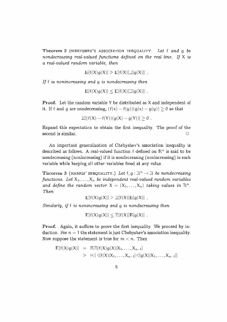
Theorem 2 chebyshev's association inequality. Let f and g be
nondecreasing real-valued functions de�ned on the real line. If X is
a real-valued random variable, then
E[f(X)g(X)] � E[f(X)]E[g(X)]| .
If f is nonincreasing and g is nondecreasing then
E[f(X)g(X)] � E[f(X)]E[g(X)]| .
Proof. Let the random variable Y be distributed as X and independent of
it. If f and g are nondecreasing, (f(x) − f(y))(g(x) − g(y)) � 0 so that
E[(f(X) − f(Y))(g(X) − g(Y))] � 0 .Expand this expectation to obtain the �rst inequality. The proof of the
second is similar. 2
An important generalization of Chebyshev's association inequality is
described as follows. A real-valued function f de�ned on Rn is said to be
nondecreasing (nonincreasing) if it is nondecreasing (nonincreasing) in each
variable while keeping all other variables �xed at any value.
Theorem 3 (harris' inequality.) Let f, g : Rn → R be nondecreasing
functions. Let X1, . . . , Xn be independent real-valued random variables
and de�ne the random vector X = (X1, . . . , Xn) taking values in Rn.
Then
E[f(X)g(X)] � E[f(X)]E[g(X)] .
Similarly, if f is nonincreasing and g is nondecreasing then
E[f(X)g(X)] � E[f(X)]E[g(X)] .
Proof. Again, it su�ces to prove the �rst inequality. We proceed by in-
duction. For n = 1 the statement is just Chebyshev's association inequality.
Now suppose the statement is true for m < n. Then
E[f(X)g(X)] = EE[f(X)g(X)|X1, . . . , Xn−1]
� E [E[f(X)|X1, . . . , Xn−1]E[g(X)|X1, . . . , Xn−1]]
5

because given X1, . . . , Xn−1, both f and g are nondecreasing functions of the
n-th variable. Now it follows by independence that the functions f 0, g 0 :
Rn−1 → R de�ned by f 0(x1, . . . .xn−1) = E[f(X)|X1 = x1, . . . , Xn−1 = xn−1]
and g 0(x1, . . . .xn−1) = E[g(X)|X1 = x1, . . . , Xn−1 = xn−1] are nondecreasing
functions, so by the induction hypothesis,
E[f 0(X1, . . . , Xn−1)g0(X1, . . . , Xn−1)]
� E[f 0(X1, . . . , Xn−1)]E[g 0(X1, . . . , Xn−1)]
= E[f(X)]E[g(X)]
as desired. 2
Exercises
Exercise 1 moments vs. chernoff bounds. Show that moment bounds
for tail probabilities are always better than Cherno� bounds. More pre-
cisely, let X be a nonnegative random variable and let t > 0. The best
moment bound for the tail probability P{X � t} is minqE[Xq]t−q where
the minimum is taken over all positive integers. The best Cherno� bound
is infs>0E[es(X−t)]. Prove that
minqE[Xq]t−q � inf
s>0E[es(X−t)].
Exercise 2 first and second moment methods. Show that if X is a
nonnegative integer-valued random variable then P{X 6= 0} � EX. Show
also that
P{X = 0} � Var(X)
Var(X) + (EX)2.
Exercise 3 subgaussian moments. We say that a random variable X has
a subgaussian distribution if there exists a constant c > 0 such that for all
s > 0, E[esX] � ecs2. Show that there exists a universal constant K such
that if X is subgaussian, then for every positive integer q,
(E[Xq+])
1/q � Kpcq .
6
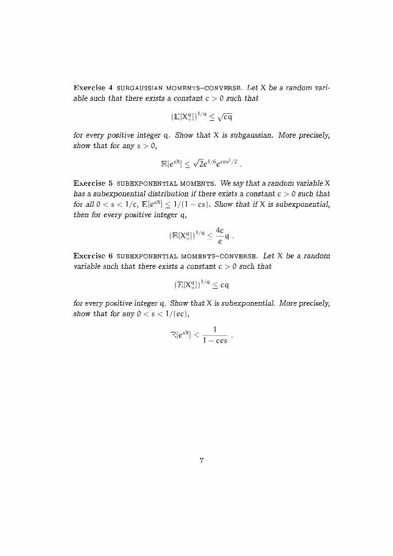
Exercise 4 subgaussian moments�converse. Let X be a random vari-
able such that there exists a constant c > 0 such that
(E[Xq+])
1/q � pcq
for every positive integer q. Show that X is subgaussian. More precisely,
show that for any s > 0,
E[esX] �p2e1/6eces2/2 .
Exercise 5 subexponential moments. We say that a random variable X
has a subexponential distribution if there exists a constant c > 0 such that
for all 0 < s < 1/c, E[esX] � 1/(1− cs). Show that if X is subexponential,
then for every positive integer q,
(E[Xq+])
1/q � 4c
eq .
Exercise 6 subexponential moments�converse. Let X be a random
variable such that there exists a constant c > 0 such that
(E[Xq+])
1/q � cq
for every positive integer q. Show that X is subexponential. More precisely,
show that for any 0 < s < 1/(ec),
E[esX] � 1
1− ces.
7
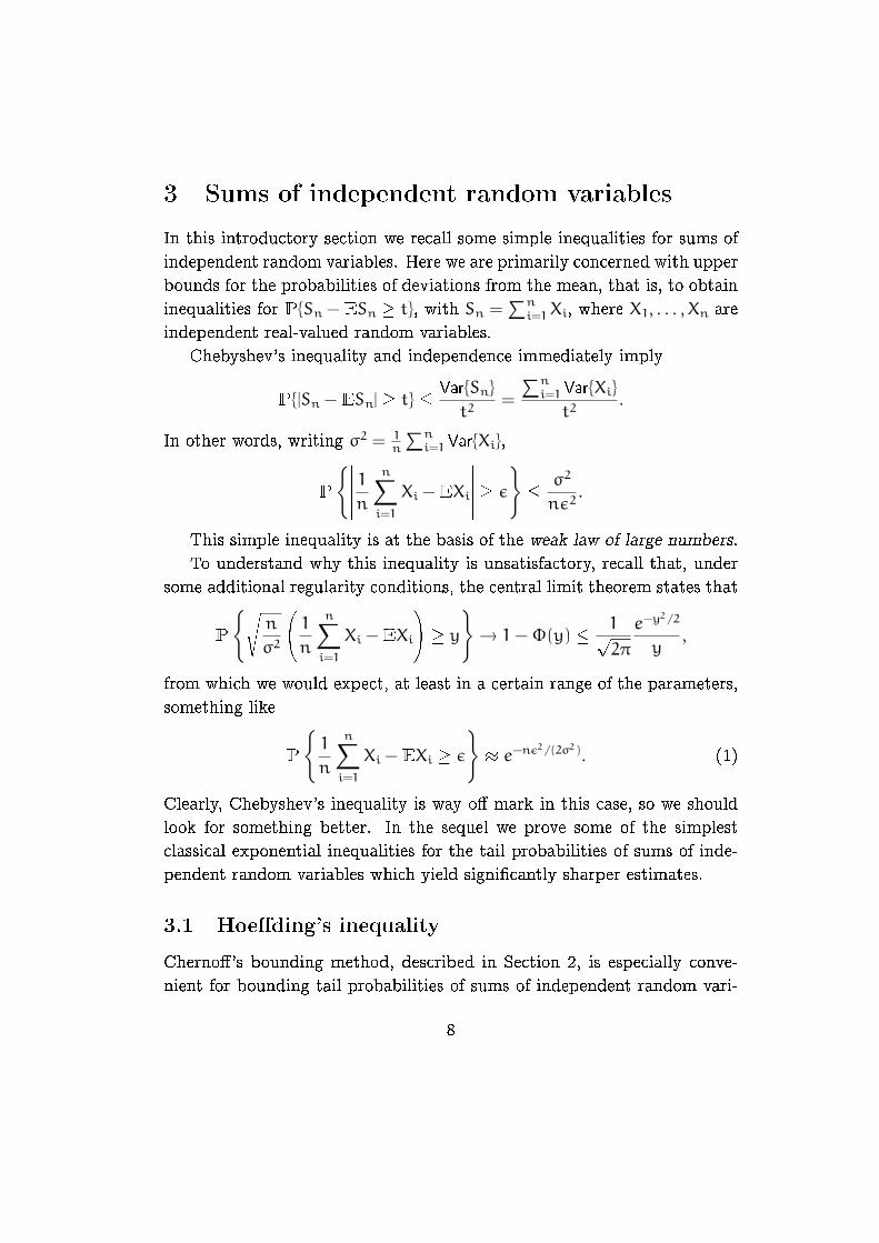
3 Sums of independent random variables
In this introductory section we recall some simple inequalities for sums of
independent random variables. Here we are primarily concerned with upper
bounds for the probabilities of deviations from the mean, that is, to obtain
inequalities for P{Sn −ESn � t}, with Sn =∑n
i=1 Xi, where X1, . . . , Xn are
independent real-valued random variables.
Chebyshev's inequality and independence immediately imply
P{|Sn −ESn| � t} � Var{Sn}
t2=
∑ni=1 Var{Xi}
t2.
In other words, writing σ2 = 1n
∑ni=1 Var{Xi},
P
{������ 1nn∑
i=1
Xi −EXi
������ � ε}� σ2
nε2.
This simple inequality is at the basis of the weak law of large numbers.
To understand why this inequality is unsatisfactory, recall that, under
some additional regularity conditions, the central limit theorem states that
P
{sn
σ2
0@ 1n
n∑i=1
Xi −EXi
1A � y} → 1−Φ(y) � 1p
2π
e−y2/2
y,
from which we would expect, at least in a certain range of the parameters,
something like
P
{1
n
n∑i=1
Xi −EXi � ε}� e−nε2/(2σ2). (1)
Clearly, Chebyshev's inequality is way o� mark in this case, so we should
look for something better. In the sequel we prove some of the simplest
classical exponential inequalities for the tail probabilities of sums of inde-
pendent random variables which yield signi�cantly sharper estimates.
3.1 Hoe�ding's inequality
Cherno�'s bounding method, described in Section 2, is especially conve-
nient for bounding tail probabilities of sums of independent random vari-
8
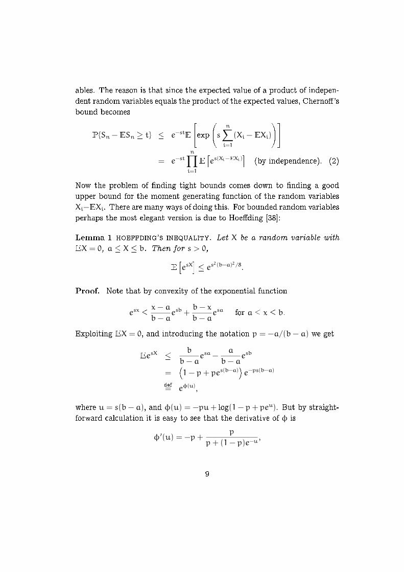
ables. The reason is that since the expected value of a product of indepen-
dent random variables equals the product of the expected values, Cherno�'s
bound becomes
P{Sn −ESn � t} � e−stE
24exp0@s n∑
i=1
(Xi −EXi)
1A35= e−st
n∏i=1
E
hes(Xi−EXi)
i(by independence). (2)
Now the problem of �nding tight bounds comes down to �nding a good
upper bound for the moment generating function of the random variables
Xi−EXi. There are many ways of doing this. For bounded random variables
perhaps the most elegant version is due to Hoe�ding [38]:
Lemma 1 hoeffding's inequality. Let X be a random variable with
EX = 0, a � X � b. Then for s > 0,
E
hesX
i� es2(b−a)2/8.
Proof. Note that by convexity of the exponential function
esx � x− a
b− aesb +
b− x
b− aesa for a � x � b.
Exploiting EX = 0, and introducing the notation p = −a/(b− a) we get
EesX � b
b− aesa −
a
b− aesb
=�1− p+ pes(b−a)
�e−ps(b−a)
def= eφ(u),
where u = s(b− a), and φ(u) = −pu+ log(1− p+ peu). But by straight-
forward calculation it is easy to see that the derivative of φ is
φ 0(u) = −p+p
p+ (1− p)e−u,
9
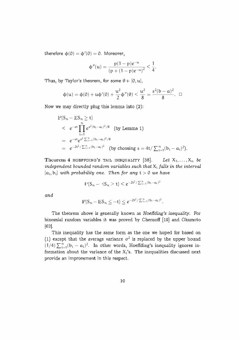
therefore φ(0) = φ 0(0) = 0. Moreover,
φ 00(u) =p(1− p)e−u
(p+ (1− p)e−u)2 �
1
4.
Thus, by Taylor's theorem, for some θ 2 [0, u],
φ(u) = φ(0) + uφ 0(0) +u2
2φ 00(θ) � u2
8=s2(b− a)2
8. 2
Now we may directly plug this lemma into (2):
P{Sn −ESn � t}
� e−stn∏
i=1
es2(bi−ai)2/8 (by Lemma 1)
= e−stes2∑n
i=1(bi−ai)2/8
= e−2t2/∑n
i=1(bi−ai)2
(by choosing s = 4t/∑n
i=1(bi − ai)2).
Theorem 4 hoeffding's tail inequality [38]. Let X1, . . . , Xn be
independent bounded random variables such that Xi falls in the interval
[ai, bi] with probability one. Then for any t > 0 we have
P{Sn −ESn � t} � e−2t2/∑n
i=1(bi−ai)2
and
P{Sn −ESn � −t} � e−2t2/∑n
i=1(bi−ai)2
.
The theorem above is generally known as Hoe�ding's inequality. For
binomial random variables it was proved by Cherno� [19] and Okamoto
[62].
This inequality has the same form as the one we hoped for based on
(1) except that the average variance σ2 is replaced by the upper bound
(1/4)∑n
i=1(bi − ai)2. In other words, Hoe�ding's inequality ignores in-
formation about the variance of the Xi's. The inequalities discussed next
provide an improvement in this respect.
10
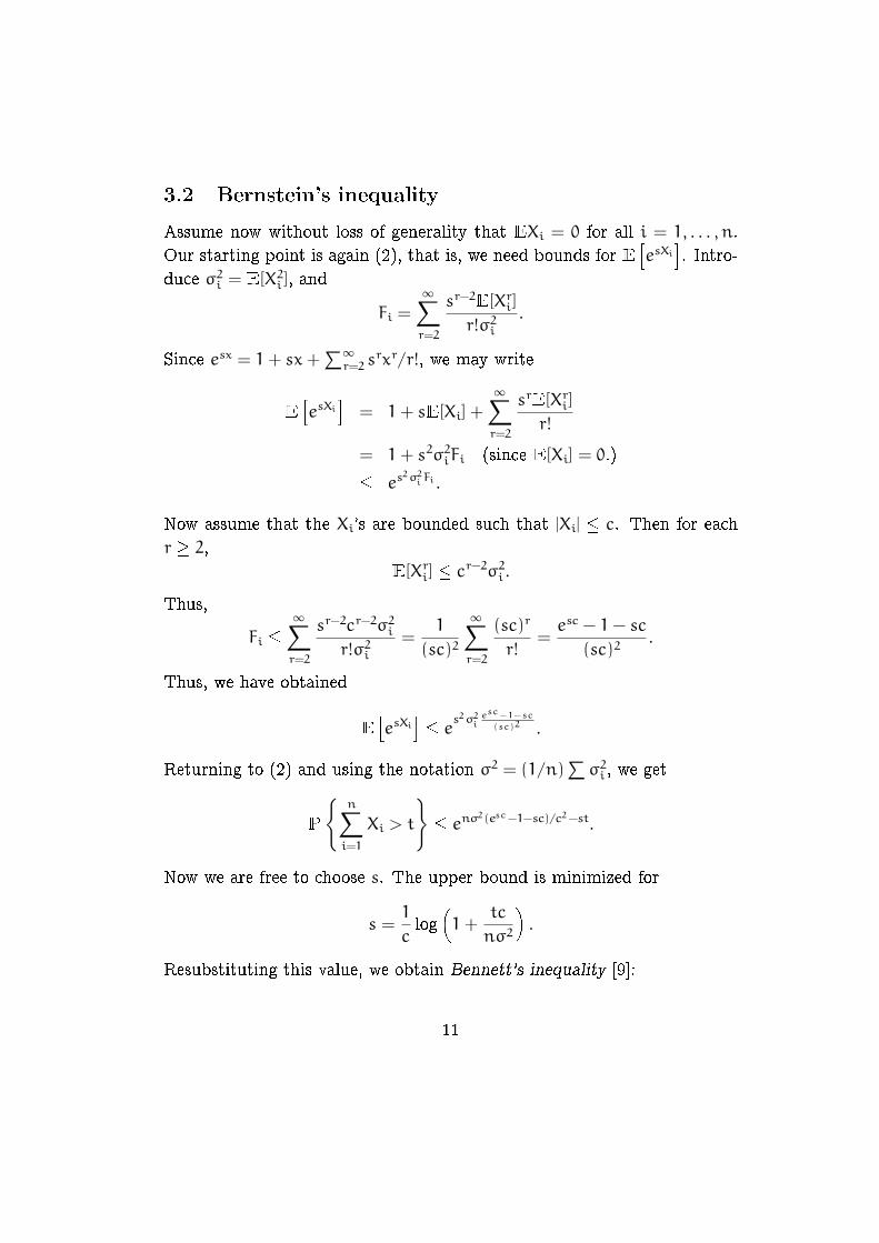
3.2 Bernstein's inequality
Assume now without loss of generality that EXi = 0 for all i = 1, . . . , n.
Our starting point is again (2), that is, we need bounds for EhesXi
i. Intro-
duce σ2i = E[X2
i ], and
Fi =
∞∑r=2
sr−2E[Xr
i ]
r!σ2i
.
Since esx = 1+ sx+∑∞
r=2 srxr/r!, we may write
E
hesXi
i= 1+ sE[Xi] +
∞∑r=2
srE[Xri ]
r!
= 1+ s2σ2iFi (since E[Xi] = 0.)
� es2σ2i Fi.
Now assume that the Xi's are bounded such that |Xi| � c. Then for each
r � 2,E[Xr
i ] � cr−2σ2i .
Thus,
Fi �∞∑
r=2
sr−2cr−2σ2i
r!σ2i
=1
(sc)2
∞∑r=2
(sc)r
r!=esc − 1− sc
(sc)2.
Thus, we have obtained
E
hesXi
i� es2σ2
iesc−1−sc
(sc)2 .
Returning to (2) and using the notation σ2 = (1/n)∑σ2
i , we get
P
{n∑
i=1
Xi > t
}� enσ2(esc−1−sc)/c2−st.
Now we are free to choose s. The upper bound is minimized for
s =1
clog
�1+
tc
nσ2
�.
Resubstituting this value, we obtain Bennett's inequality [9]:
11
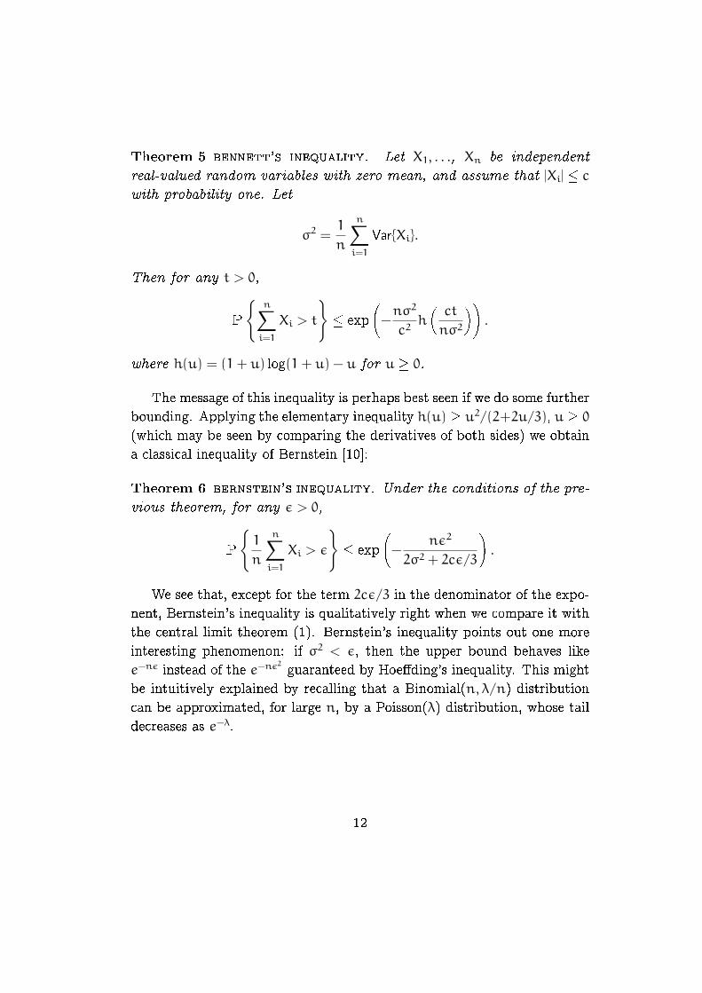
Theorem 5 bennett's inequality. Let X1, . . ., Xn be independent
real-valued random variables with zero mean, and assume that |Xi| � cwith probability one. Let
σ2 =1
n
n∑i=1
Var{Xi}.
Then for any t > 0,
P
{n∑
i=1
Xi > t
}� exp
−nσ2
c2h
�ct
nσ2
�!.
where h(u) = (1+ u) log(1+ u) − u for u � 0.
The message of this inequality is perhaps best seen if we do some further
bounding. Applying the elementary inequality h(u) � u2/(2+2u/3), u � 0(which may be seen by comparing the derivatives of both sides) we obtain
a classical inequality of Bernstein [10]:
Theorem 6 bernstein's inequality. Under the conditions of the pre-
vious theorem, for any ε > 0,
P
{1
n
n∑i=1
Xi > ε
}� exp
−
nε2
2σ2 + 2cε/3
!.
We see that, except for the term 2cε/3 in the denominator of the expo-
nent, Bernstein's inequality is qualitatively right when we compare it with
the central limit theorem (1). Bernstein's inequality points out one more
interesting phenomenon: if σ2 < ε, then the upper bound behaves like
e−nε instead of the e−nε2guaranteed by Hoe�ding's inequality. This might
be intuitively explained by recalling that a Binomial(n, λ/n) distribution
can be approximated, for large n, by a Poisson(λ) distribution, whose tail
decreases as e−λ.
12
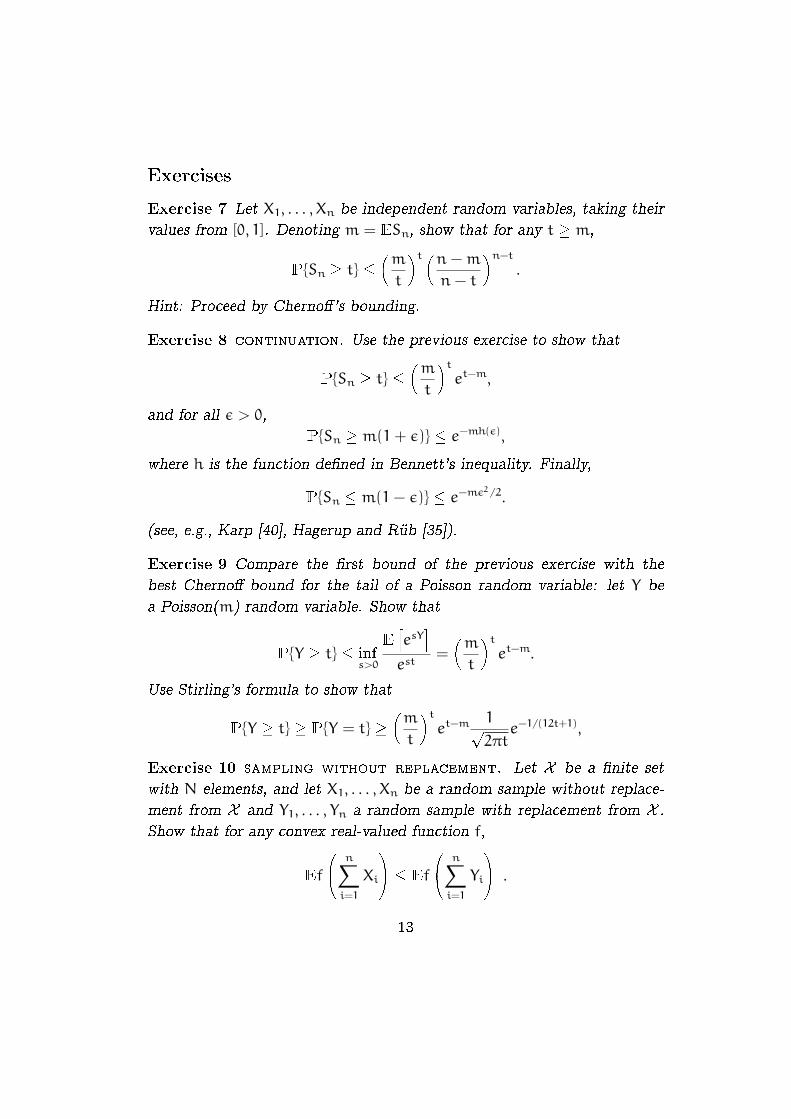
Exercises
Exercise 7 Let X1, . . . , Xn be independent random variables, taking their
values from [0, 1]. Denoting m = ESn, show that for any t � m,
P{Sn � t} ��m
t
�t �n−m
n− t
�n−t
.
Hint: Proceed by Cherno�'s bounding.
Exercise 8 continuation. Use the previous exercise to show that
P{Sn � t} ��m
t
�t
et−m,
and for all ε > 0,
P{Sn � m(1+ ε)} � e−mh(ε),
where h is the function de�ned in Bennett's inequality. Finally,
P{Sn � m(1− ε)} � e−mε2/2.
(see, e.g., Karp [40], Hagerup and Rüb [35]).
Exercise 9 Compare the �rst bound of the previous exercise with the
best Cherno� bound for the tail of a Poisson random variable: let Y be
a Poisson(m) random variable. Show that
P{Y � t} � infs>0
E
hesYi
est=
�m
t
�t
et−m.
Use Stirling's formula to show that
P{Y � t} � P{Y = t} ��m
t
�t
et−m 1p2πt
e−1/(12t+1),
Exercise 10 sampling without replacement. Let X be a �nite set
with N elements, and let X1, . . . , Xn be a random sample without replace-
ment from X and Y1, . . . , Yn a random sample with replacement from X .
Show that for any convex real-valued function f,
Ef
0@ n∑i=1
Xi
1A � Ef0@ n∑
i=1
Yi
1A .
13

In particular, by taking f(x) = esx, we see that all inequalities derived for
the sums of independent random variables Yi using Cherno�'s bounding
remain true for the sum of the Xi's. (This result is due to Hoe�ding [38].)
14
4 The Efron-Stein inequality
The main purpose of these notes is to show how many of the tail inequali-
ties for sums of independent random variables can be extended to general
functions of independent random variables. The simplest, yet surprisingly
powerful inequality of this kind is known as the Efron-Stein inequality. It
bounds the variance of a general function. To obtain tail inequalities, one
may simply use Chebyshev's inequality.
Let X be some set, and let g : X n → R be a measurable function of
n variables. We derive inequalities for the di�erence between the random
variable Z = g(X1, . . . , Xn) and its expected value EZ when X1, . . . , Xn are
arbitrary independent (not necessarily identically distributed!) random
variables taking values in X .
The main inequalities of this section follow from the next simple result.
To simplify notation, we write Ei for the expected value with respect to
the variable Xi, that is, EiZ = E[Z|X1, . . . , Xi−1, Xi+1, . . . , Xn].
Theorem 7
Var(Z) �n∑
i=1
E
h(Z−EiZ)
2i.
Proof. The proof is based on elementary properties of conditional ex-
pectation. Recall that if X and Y are arbitrary bounded random variables,
then E[XY] = E[E[XY|Y]] = E[YE[X|Y]].
Introduce the notation V = Z−EZ, and de�ne
Vi = E[Z|X1, . . . , Xi] −E[Z|X1, . . . , Xi−1], i = 1, . . . , n.
Clearly, V =∑n
i=1 Vi. (Thus, V is written as a sum of martingale di�er-
15
ences.) Then
Var(Z) = E
2640@ n∑
i=1
Vi
1A2375
= E
n∑i=1
V2i + 2E
∑i>j
ViVj
= E
n∑i=1
V2i ,
since, for any i > j,
EViVj = EE [ViVj|X1, . . . , Xj] = E [VjE [Vi|X1, . . . , Xj]] = 0 .
To bound EV2i , note that, by independence of the Xi,
E[Z|X1, . . . , Xi−1] = E
�E[Z|X1, . . . , Xi−1, Xi+1, . . . , Xn]
����X1, . . . , Xi
�,
and therefore
V2i = (E[Z|X1, . . . , Xi] −E[Z|X1, . . . , Xi−1])
2
=
�E
�E[Z|X1, . . . , Xn] −E[Z|X1, . . . , Xi−1, Xi+1, . . . , Xn]
����X1, . . . , Xi
��2
� E
�(E[Z|X1, . . . , Xn] −E[Z|X1, . . . , Xi−1, Xi+1, . . . , Xn])
2����X1, . . . , Xi
�(by Jensen's inequality)
= E
�(Z−EiZ)
2����X1, . . . , Xi
�.
Taking expected values on both sides, we obtain the statement. 2
Now the Efron-Stein inequality follows easily. To state the theorem, let
X 01, . . . , X0n form an independent copy of X1, . . . , Xn and write
Z 0i = g(X1, . . . , X0i, . . . , Xn) .
Theorem 8 efron-stein inequality (efron and stein [32], steele
[73]).
Var(Z) � 1
2
n∑i=1
E
h(Z− Z 0i)
2i
16
Proof. The statement follows by Theorem 7 simply by using (condition-
ally) the elementary fact that if X and Y are independent and identically
distributed random variables, then Var(X) = (1/2)E[(X−Y)2], and therefore
Ei
h(Z−EiZ)
2i
=1
2Ei
h(Z− Z 0i)
2i. 2
Remark. Observe that in the case when Z =∑n
i=1 Xi is a sum of indepen-
dent random variables (of �nite variance) then the inequality in Theorem
8 becomes an equality. Thus, the bound in the Efron-Stein inequality is,
in a sense, not improvable. This example also shows that, among all func-
tions of independent random variables, sums, in some sense, are the least
concentrated. Below we will see other evidences for this extremal property
of sums.
Another useful corollary of Theorem 7 is obtained by recalling that, for
any random variable X, Var(X) � E[(X−a)2] for any constant a 2 R. Usingthis fact conditionally, we have, for every i = 1, . . . , n,
Ei
h(Z−EiZ)
2i� Ei
h(Z− Zi)
2i
where Zi = gi(X1, . . . , Xi−1, Xi+1, . . . , Xn) for arbitrary measurable functions
gi : X n−1 → R of n − 1 variables. Taking expected values and using
Theorem 7 we have the following.
Theorem 9
Var(Z) �n∑
i=1
E
h(Z− Zi)
2i.
In the next two sections we specialize the Efron-Stein inequality and
its variant Theorem 9 to functions which satisfy some simple easy-to-verify
properties.
4.1 Functions with bounded di�erences
We say that a function g : X n → R has the bounded di�erences property
if for some nonnegative constants c1, . . . , cn,
supx1,...,xn,
x 0
i2X
|g(x1, . . . , xn) − g(x1, . . . , xi−1, x0i, xi+1, . . . , xn)| � ci , 1 � i � n .
17
In other words, if we change the i-th variable of g while keeping all the
others �xed, the value of the function cannot change by more than ci.
Then the Efron-Stein inequality implies the following:
Corollary 1 If g has the bounded di�erences property with constants
c1, . . . , cn, then
Var(Z) � 1
2
n∑i=1
c2i .
Next we list some interesting applications of this corollary. In all cases
the bound for the variance is obtained e�ortlessly, while a direct estimation
of the variance may be quite involved.
Example. bin packing. This is one of the basic operations research
problems. Given n numbers x1, . . . , xn 2 [0, 1], the question is the fol-
lowing: what is the minimal number of �bins� into which these numbers
can be packed such that the sum of the numbers in each bin doesn't ex-
ceed one. Let g(x1, . . . , xn) be this minimum number. The behavior of
Z = g(X1, . . . , Xn), when X1, . . . , Xn are independent random variables, has
been extensively studied, see, for example, Rhee and Talagrand [67], Rhee
[66], Talagrand [75]. Now clearly by changing one of the xi's, the value of
g(x1, . . . , xn) cannot change by more than one, so we have
Var(Z) � n
2.
However, sharper bounds may be proved by using Talagrand's convex dis-
tance inequality discussed later.
Example. longest common subsequence. This problem has been
studied intensively for about 20 years now, see Chvátal and Sanko� [20],
Deken [23], Dan£ík and Paterson [22], Steele [72, 74], The simplest version
is the following: Let X1, . . . , Xn and Y1, . . . , Yn be two sequences of coin
�ips. De�ne Z as the length of the longest subsequence which appears in
both sequences, that is,
Z = max{k : Xi1 = Yj1, . . . , Xik = Yjk,
where 1 � i1 < � � � < ik � n and 1 � j1 < � � � < jk � n}.
18
The behavior of EZ has been investigated in many papers. It is known
that E[Z]/n converges to some number γ, whose value is unknown. It
is conjectured to be 2/(1 +p2), and it is known to fall between 0.75796
and 0.83763. Here we are concerned with the concentration of Z. A mo-
ment's thought reveals that changing one bit can't change the length of the
longest common subsequence by more than one, so Z satis�es the bounded
di�erences property with ci = 1. Consequently,
Var{Z} � n,
(see Steele [73]). Thus, by Chebyshev's inequality, with large probability,
Z is within a constant timespn of its expected value. In other words, it
is strongly concentrated around the mean, which means that results about
EZ really tell us about the behavior of the longest common subsequence
of two random strings.
Example. uniform deviations. One of the central quantities of sta-
tistical learning theory and empirical process theory is the following: let
X1, . . . , Xn be i.i.d. random variables taking their values in some set X , and
let A be a collection of subsets of X . Let µ denote the distribution of X1,
that is, µ(A) = P{X1 2 A}, and let µn denote the empirical distribution:
µn(A) =1
n
n∑i=1
1{Xi2A} .
The quantity of interest is
Z = supA2A
|µn(A) − µ(A)|.
If limn→∞EZ = 0 for every distribution of the Xi's, then A is called a
uniform Glivenko-Cantelli class, and Vapnik and Chervonenkis [81] gave a
beautiful combinatorial characterization of such classes. But regardless of
what A is, by changing one Xi, Z can change by at most 1/n, so regardless
of the behavior of EZ, we always have
Var(Z) � 1
2n.
19
For more information on the behavior of Z and its role in learning theory
see, for example, Devroye, Györ�, and Lugosi [28], Vapnik [80], van der
Vaart and Wellner [78], Dudley [31].
Next we show how a closer look at the Efron-Stein inequality implies a
signi�cantly better bound for the variance of Z. We do this in a slightly
more general framework of empirical processes. Let F be a class of real-
valued functions (no boundedness is assumed!) and de�ne Z = g(X1, . . . , Xn) =
supf2F
∑nj=1 f(Xj). Observe that, by symmetry, the Efron-Stein inequality
may be rewritten as
Var(Z) � 1
2
n∑i=1
E
h(Z− Z 0i)
2i
=
n∑i=1
E
h(Z− Z 0i)
21Z 0
i<Z
i.
Let f� 2 F denote the (random) function which achieves the supremum in
the de�nition of Z, that is, Z =∑n
j=1 f�(Xj). Then clearly,
(Z− Z 0i)21Z 0
i<Z � (f�(Xi) − f�(X 0i))2
and therefore
Var(Z) � E
24supf2F
n∑i=1
(f(Xi) − f(X 0i))2
35� E
24supf2F
n∑i=1
�2f(Xi)
2 + 2f(X 0i)2�35
� 4E
24supf2F
n∑i=1
f(Xi)2
35 .For functions f 2 F are taking values in the interval [−1, 1], then from just
the bounded di�erences property we derived Var(Z) � 2n. The new bound
may be a signi�cant improvement whenever the maximum of the variances∑ni=1 f(Xi)
2 of the functions in F is small. More importantly, in deriving
the new bound we have not assumed any boundedness of the functions f.
The exponential tail inequality due to Talagrand [76] extends this variance
inequality, and is one of the most important recent results of the theory
of empirical processes, see also Ledoux [45], Massart [56], Rio [68], and
Bousquet [16].
20
Example. first passage time in oriented percolation. Consider a
directed graph such that a weight Xi is assigned to each edge ei such that
the Xi are nonnegative independent random variables with second moment
EX2i = σ2. Let v1 and v2 be �xed vertices of the graph. We are interested
in the total weight of the path from v1 to v2 with minimum weight. Thus,
Z = minP
∑ei2P
Xi
where the minimum is taken over all paths P from v1 to v2. Denote the
optimal path by P�. By replacing Xi with X0i, the total minimum weight
can only increase if the edge ei is on P�, and therefore
(Zi − Z 0i)21Z 0
i>Z � (X 0i − Xi)21ei2P� � X 0i21ei2P� .
Thus,
Var(Z) � E∑
i
X 0i21ei2P� = σ2
E
∑i
1ei2P� � σ2L
where L is the length of the longest path between v1 and v2.
Example. minimum of the empirical loss. Concentration inequalities
have been used as a key tool in recent developments of model selection
methods in statistical learning theory. For the background we refer to
the the recent work of Koltchinskii Panchenko [42], Massart [57], Bartlett,
Boucheron, and Lugosi [5], Lugosi and Wegkamp [51], Bousquet [17].
Let F denote a class of {0, 1}-valued functions on some space X . For
simplicity of the exposition we assume that F is �nite. The results remain
true for general classes as long as the measurability issues are taken care
of. Given an i.i.d. sample Dn = (hXi, Yii)i�n of n pairs of random variables
hXi, Yii taking values in X � {0, 1}, for each f 2 F we de�ne the empirical
loss
Ln(f) =1
n
n∑i=1
`(f(Xi), Yi)
where the loss function ` is de�ned on {0, 1}2 by
`(y, y 0) = 1y6=y 0 .
21
In nonparametric classi�cation and learning theory it is common to select
an element of F by minimizing the empirical loss. The quantity of interest
in this section is the minimal empirical loss
bL = inff2F
Ln(f).
Corollary 1 immediately implies that Var(bL) � 1/(2n). However, a more
careful application of the Efron-Stein inequality reveals that bLmay be much
more concentrated than predicted by this simple inequality. Getting tight
results for the �uctuations of bL provides better insight into the calibration
of penalties in certain model selection methods.
Let Z = nbL and let Z 0i be de�ned as in Theorem 8, that is,
Z 0i = minf2F
24∑j6=i
`(f(Xj), Yj) + `(f(Xi0), Yi
0)
35where hXi
0, Yi0i is independent of Dn and has the same distribution as
hXi, Yii. Now the convenient form of the Efron-Stein inequality is the fol-
lowing:
Var(Z) � 1
2
n∑i=1
E
h(Z− Z 0i)
2i
=
n∑i=1
E
h(Z− Z 0i)
21Z 0
i>Z
iLet f� denote a (possibly non-unique) minimizer of the empirical risk so
that Z =∑n
j=1 `(f�(Xj), Yj). The key observation is that
(Z− Z 0i)21Z 0
i>Z � (`(f�(Xi0), Yi
0) − `(f�(Xi), Yi))21Z 0
i>Z
= `(f�(X 0i), Y0i)1`(f�(Xi),Yi)=0 .
Thus,
n∑i=1
E
h(Z− Z 0i)
21Z 0
i>Z
i� E
∑i:`(f�(Xi),Yi)=0
EX 0
i,Y0
i[`(f�(X 0i), Y
0i)] � nEL(f�)
where EX 0
i,Y0
idenotes expectation with respect to the variables X 0i, Y
0i and for
each f 2 F , L(f) = E`(f(X), Y) is the true (expected) loss of f. Therefore,
the Efron-Stein inequality implies that
Var(bL) � EL(f�)
n.
22
This is a signi�cant improvement over the bound 1/(2n) whenever EL(f�)
is much smaller than 1/2. This is very often the case. For example, we
have
L(f�) = bL− (Ln(f�) − L(f�)) � Z
n+ sup
f2F(L(f) − Ln(f))
so that we obtain
Var(bL) � EbLn
+E supf2F(L(f) − Ln(f))
n.
In most cases of interest, E supf2F(L(f) − Ln(f)) may be bounded by a
constant (depending on F) times n−1/2 (see, e.g., Lugosi [50]) and then the
second term on the right-hand side is of the order of n−3/2. For exponential
concentration inequalities for bL we refer to Boucheron, Lugosi, and Massart
[15].
Example. kernel density estimation. Let X1, . . . , Xn be i.i.d. samples
drawn according to some (unknown) density f on the real line. The density
is estimated by the kernel estimate
fn(x) =1
nh
n∑i=1
K
x− Xi
h
!,
where h > 0 is a smoothing parameter, and K is a nonnegative function
with∫K = 1. The performance of the estimate is measured by the L1 error
Z = g(X1, . . . , Xn) =
∫|f(x) − fn(x)|dx.
It is easy to see that
|g(x1, . . . , xn) − g(x1, . . . , x0i, . . . , xn)| � 1
nh
∫ �����K�x− xi
h
�− K
x− x 0ih
!�����dx� 2
n,
so without further work we get
Var(Z) � 2
n.
23

It is known that for every f,pnEg → ∞ (see Devroye and Györ� [27])
which implies, by Chebyshev's inequality, that for every ε > 0
P
{����� ZEZ − 1
����� � ε}
= P {|Z−EZ| � εEZ} � Var(Z)
ε2(EZ)2→ 0
as n → ∞. That is, Z/EZ → 0 in probability, or in other words, Z is
relatively stable. This means that the random L1-error behaves like its
expected value. This result is due to Devroye [25], [26]. For more on the
behavior of the L1 error of the kernel density estimate we refer to Devroye
and Györ� [27], Devroye and Lugosi [29].
4.2 Self-bounding functions
Another simple property which is satis�ed for many important examples is
the so-called self-bounding property. We say that a nonnegative function
g : X n → R has the self-bounding property if there exist functions gi :
X n−1 → R such that for all x1, . . . , xn 2 X and all i = 1, . . . , n,
0 � g(x1, . . . , xn) − gi(x1, . . . , xi−1, xi+1, . . . , xn) � 1
and also
n∑i=1
(g(x1, . . . , xn) − gi(x1, . . . , xi−1, xi+1, . . . , xn)) � g(x1, . . . , xn) .
Concentration properties for such functions have been studied by Boucheron,
Lugosi, and Massart [14], Rio [68], and Bousquet [16]. For self-bounding
functions we clearly have
n∑i=1
(g(x1, . . . , xn) − gi(x1, . . . , xi−1, xi+1, . . . , xn))2 � g(x1, . . . , xn) .
and therefore Theorem 9 implies
Corollary 2 If g has the self-bounding property, then
Var(Z) � EZ .
24
Next we mention some applications of this simple corollary. It turns
out that in many cases the obtained bound is a signi�cant improvement
over what we would obtain by using simply Corollary 1.
Remark. relative stability. Bounding the variance of Z by its ex-
pected value implies, in many cases, the relative stability of Z. A se-
quence of nonnegative random variables (Zn) is said to be relatively stable
if Zn/EZn → 1 in probability. This property guarantees that the random
�uctuations of Zn around its expectation are of negligible size when com-
pared to the expectation, and therefore most information about the size
of Zn is given by EZn. If Zn has the self-bounding property, then, by
Chebyshev's inequality, for all ε > 0,
P
{����� Zn
EZn
− 1
����� > ε}� Var(Zn)
ε2(EZn)2� 1
ε2EZn
.
Thus, for relative stability, it su�ces to have EZn → ∞.
Example. empirical processes. A typical example of self-bounding
functions is the supremum of nonnegative empirical processes. Let Fbe a class of functions taking values in the interval [0, 1] and consider
Z = g(X1, . . . , Xn) = supf2F
∑nj=1 f(Xj). (A special case of this is men-
tioned above in the example of uniform deviations.) De�ning gi = g 0
for i = 1, . . . , n with g 0(x1, . . . , xn−1) = supf2F
∑n−1j=1 f(Xj) (so that Zi =
supf2F
∑nj=1
j6=if(Xj)) and letting f
� 2 F be a function for which Z =∑n
j=1 f�(Xj),
one obviously has
0 � Z− Zi � f�(Xi) � 1and therefore
n∑i=1
(Z− Zi) �n∑
i=1
f�(Xi) = Z.
(Here we have assumed that the supremum is always achieved. The mod-
i�cation of the argument for the general case is straightforward.) Thus,
by Corollary 2 we obtain Var(Z) � EZ. Note that Corollary 1 implies
Var(Z) � n/2. In some important applications EZ may be signi�cantly
smaller than n/2 and the improvement is essential.
25

Example. rademacher averages. A less trivial example for self-
bounding functions is the one of Rademacher averages. Let F be a class of
functions with values in [−1, 1]. If σ1, . . . , σn denote independent symmet-
ric {−1, 1}-valued random variables, independent of the Xi's (the so-called
Rademacher random variables), then we de�ne the conditional Rademacher
average as
Z = E
24supf2F
n∑j=1
σjf(Xj)|Xn1
35 .(Thus, the expected value is taken with respect to the Rademacher variables
and Z is a function of the Xi's.) Quantities like Z have been known to
measure e�ectively the complexity of model classes in statistical learning
theory, see, for example, Koltchinskii [41], Bartlett, Boucheron, and Lugosi
[5], Bartlett and Mendelson [7], Bartlett, Bousquet, and Mendelson [6]. It
is immediate that Z has the bounded di�erences property and Corollary 1
implies Var(Z) � n/2. However, this bound may be improved by observing
that Z also has the self-bounding property, and therefore Var(Z) � EZ.
Indeed, de�ning
Zi = E
26664supf2F
n∑j=1
j6=i
σjf(Xj)|Xn1
37775it is easy to see that 0 � Z−Zi � 1 and
∑ni=1(Z−Zi) � Z (the details are
left as an exercise). The improvement provided by Lemma 2 is essential
since it is well-known in empirical process theory and statistical learning
theory that in many cases when F is a relatively small class of functions, EZ
may be bounded by something like Cn1/2 where the constant C depends on
the class F , see, e.g., Vapnik [80], van der Vaart and Wellner [78], Dudley
[31].
Con�guration functions
An important class of functions satisfying the self-bounding property con-
sists of the so-called con�guration functions de�ned by Talagrand [75, sec-
tion 7]. Our de�nition, taken from [14] is a slight modi�cation of Tala-
grand's.
26
Assume that we have a property P de�ned over the union of �nite
products of a set X , that is, a sequence of sets P1 � X , P2 � X�X , . . . , Pn �X n. We say that (x1, . . . xm) 2 Xm satis�es the property P if (x1, . . . xm) 2Pm. We assume that P is hereditary in the sense that if (x1, . . . xm) satis�es
P then so does any subsequence (xi1, . . . xik) of (x1, . . . xm). The function
gn that maps any tuple (x1, . . . xn) to the size of a largest subsequence
satisfying P is the con�guration function associated with property P.
Corollary 2 implies the following result:
Corollary 3 Let gn be a con�guration function, and let Z = gn(X1, . . . , Xn),
where X1, . . . , Xn are independent random variables. Then
Var(Z) � EZ .
Proof. By Corollary 2 it su�ces to show that any con�guration function
is self bounding. Let Zi = gn−1(X1, . . . , Xi−1, Xi+1, . . . , Xn). The condition
0 � Z−Zi � 1 is trivially satis�ed. On the other hand, assume that Z = k
and let {Xi1, . . . , Xik} � {X1, . . . , Xn} be a subsequence of cardinality k such
that fk(Xi1, . . . , Xik) = k. (Note that by the de�nition of a con�guration
function such a subsequence exists.) Clearly, if the index i is such that
i /2 {i1, . . . , ik} then Z = Zi, and therefore
n∑i=1
(Z− Zi) � Z
is also satis�ed, which concludes the proof. 2
To illustrate the fact that con�guration functions appear rather natu-
rally in various applications, we describe some examples originating from
di�erent �elds.
Example. number of distinct values in a discrete sample. Let
X1, . . . , Xn be independent, identically distributed random variables taking
their values on the set of positive integers such that P{X1 = k} = pk, and let
Z denote the number of distinct values taken by these n random variables.
Then we may write
Z =
n∑i=1
1{Xi 6=X1,...,Xi 6=Xi−1},
27
so the expected value of Z may be computed easily:
EZ =
n∑i=1
∞∑j=1
(1− pj)i−1pj.
It is easy to see that E[Z]/n → 0 as n → ∞ (see Exercise 13). But how
concentrated is the distribution of Z? Clearly, Z satis�es the bounded
di�erences property with ci = 1, so Corollary 1 implies Var(Z) � n/2 so
Z/n → 0 in probability by Chebyshev's inequality. On the other hand, it
is obvious that Z is a con�guration function associated to the property of
�distinctness�, and by Corollary 3 we have
Var(Z) � EZ
which is a signi�cant improvement since EZ = o(n).
Example. vc dimension. One of the central quantities in statistical
learning theory is the Vapnik-Chervonenkis dimension, see Vapnik and
Chervonenkis [81, 82], Blumer, Ehrenfeucht, Haussler, and Warmuth [11],
Devroye, Györ�, and Lugosi [28], Anthony and Bartlett [3], Vapnik [80],
etc.
LetA be an arbitrary collection of subsets of X , and let xn1 = (x1, . . . , xn)
be a vector of n points of X . De�ne the trace of A on xn1 by
tr(xn1 ) = {A \ {x1, . . . , xn} : A 2 A} .
The shatter coe�cient, (or Vapnik-Chervonenkis growth function) of A in
xn1 is T(xn
1 ) = |tr(xn1 )|, the size of the trace. T(xn
1 ) is the number of di�erent
subsets of the n-point set {x1, . . . , xn} generated by intersecting it with
elements of A. A subset {xi1, . . . , xik} of {x1, . . . , xn} is said to be shattered
if 2k = T(xi1, . . . , xik). The vc dimension D(xn1 ) of A (with respect to xn
1 ) is
the cardinality k of the largest shattered subset of xn1 . From the de�nition
it is obvious that gn(xn1 ) = D(xn
1 ) is a con�guration function (associated to
the property of �shatteredness�, and therefore if X1, . . . , Xn are independent
random variables, then
Var(D(Xn1 )) � ED(Xn
1 ) .
28
Example. increasing subsequences. Consider a vector xn1 = (x1, . . . , xn)
of n di�erent numbers in [0, 1]. The positive integers i1 < i2 < � � � < im
form an increasing subsequence if xi1 < xi2 < � � � < xim (where i1 � 1
and im � n). Let L(xn1 ) denote the length of a longest increasing subse-
quence. gn(xn1 ) = L(xn
1 ) is a clearly a con�guration function (associated
with the �increasing sequence� property), and therefore if X1, . . . , Xn are
independent random variables such that they are di�erent with probability
one (it su�ces if every Xi has an absolutely continuous distribution) then
Var(L(Xn1 )) � EL(Xn
1 ). If the Xi's are uniformly distributed in [0, 1] then it
is known that EL(Xn1 ) ∼ 2
pn, see Logan and Shepp [48], Groeneboom [34].
The obtained bound for the variance is apparently loose. A di�cult result
of Baik, Deift, and Johansson [4] implies that Var(L(Xn1 )) = O(n1/3).
For early work on the concentration on L(X) we refer to Frieze [33],
Bollobás and Brightwell [13], and Talagrand [75].
Exercises
Exercise 11 Assume that the random variables X1, . . . , Xn are indepen-
dent and binary {0,1}-valued with P{Xi = 1} = pi and that g has the
bounded di�erences property with constants c1, . . . , cn. Show that
Var(Z) �n∑
i=1
c2ipi(1− pi).
Exercise 12 Complete the proof of the fact that the conditional Rademacher
average has the self-bounding property.
Exercise 13 Consider the example of the number of distinct values in a
discrete sample described in the text. Show that E[Z]/n → 0 as n → ∞.
Calculate explicitely Var(Z) and compare it with the upper bound obtained
by Theorem 9.
Exercise 14 Let Z be the number of triangles in a random graph G(n, p).
Calculate the variance of Z and compare it with what you get by using the
Efron-Stein inequality to estimate it. (In the G(n, p) model for random
graphs, the random graph G = (V, E) with vertex set V (|V | = n) and edge
29
set E is generated by starting from the complete graph with n vertices and
deleting each edge independently from the others with probability 1 − p.
A triangle is a complete three-vertex subgraph.)
30
5 The entropy method
In the previous section we saw that the Efron-Stein inequality serves as a
powerful tool for bounding the variance of general functions of indepen-
dent random variables. Then, via Chebyshev's inequality, one may easily
bound the tail probabilities of such functions. However, just as in the case
of sums of independent random variables, tail bounds based on inequalities
for the variance are often not satisfactory, and essential improvements are
possible. The purpose of this section is to present a methodology which
allows one to obtain exponential tail inequalities in many cases. The pur-
suit of such inequalities has been an important topics in probability theory
in the last few decades. Originally, martingale methods dominated the re-
search (see, e.g., McDiarmid [58], [59], Rhee and Talagrand [67], Shamir
and Spencer [70]) but independently information-theoretic methods were
also used with success (see Alhswede, Gács, and Körner [1], Marton [52],
[53],[54], Dembo [24], Massart [55], Rio [68], and Samson [69]). Talagrand's
induction method [77],[75],[76] caused an important breakthrough both in
the theory and applications of exponential concentration inequalities. In
this section we focus on so-called �entropy method�, based on logarithmic
Sobolev inequalities developed by Ledoux [45],[44], see also Bobkov and
Ledoux [12], Massart [56], Rio [68], Boucheron, Lugosi, and Massart [14],
[15], and Bousquet [16]. This method makes it possible to derive exponen-
tial analogues of the Efron-Stein inequality perhaps the simplest way.
The method is based on an appropriate modi�cation of the �tensoriza-
tion� inequality Theorem 7. In order to prove this modi�cation, we need to
recall some of the basic notions of information theory. To keep the material
at an elementary level, we prove the modi�ed tensorization inequality for
discrete random variables only. The extension to arbitrary distributions is
straightforward.
5.1 Basic information theory
In this section we summarize some basic properties of the entropy of a
discrete-valued random variable. For a good introductory book on infor-
mation theory we refer to Cover and Thomas [21].
31
Let X be a random variable taking values in the countable set X with
distribution P{X = x} = p(x), x 2 X . The entropy of X is de�ned by
H(X) = E[− log p(X)] = −∑x2X
p(x) log p(x)
(where log denotes natural logarithm and 0 log 0 = 0). If X, Y is a pair of
discrete random variables taking values in X � Y then the joint entropy
H(X, Y) of X and Y is de�ned as the entropy of the pair (X, Y). The condi-
tional entropy H(X|Y) is de�ned as
H(X|Y) = H(X, Y) −H(Y) .
Observe that if we write p(x, y) = P{X = x, Y = y} and p(x|y) = P{X =
x|Y = y} then
H(X|Y) = −∑
x2X ,y2Y
p(x, y) log p(x|y)
from which we see that H(X|Y) � 0. It is also easy to see that the de�ning
identity of the conditional entropy remains true conditionally, that is, for
any three (discrete) random variables X, Y, Z,
H(X, Y|Z) = H(Y|Z) +H(X|Y, Z) .
(Just add H(Z) to both sides and use the de�nition of the conditional
entropy.) A repeated application of this yields the chain rule for entropy:
for arbitrary discrete random variables X1, . . . , Xn,
H(X1, . . . , Xn) = H(X1)+H(X2|X1)+H(X3|X1, X2)+� � �+H(Xn|X1, . . . , Xn−1) .
Let P and Q be two probability distributions over a countable set X with
probability mass functions p and q. Then the Kullback-Leibler divergence
or relative entropy of P and Q is
D(PkQ) =∑x2X
p(x) logp(x)
q(x).
Since log x � x− 1,
D(PkQ) = −∑x2X
p(x) logq(x)
p(x)� −
∑x2X
p(x)
q(x)
p(x)− 1
!= 0 ,
32
so that the relative entropy is always nonnegative, and equals zero if and
only if P = Q. This simple fact has some interesting consequences. For
example, if X is a �nite set with N elements and X is a random variable
with distribution P and we take Q to be the uniform distribution over Xthen D(PkQ) = logN−H(X) and therefore the entropy of X never exceeds
the logarithm of the cardinality of its range.
Consider a pair of random variables X, Y with joint distribution PX,Y and
marginal distributions PX and PY. Noting that D(PX,YkPX � PY) = H(X) −
H(X|Y), the nonnegativity of the relative entropy implies that H(X) �H(X|Y), that is, conditioning reduces entropy. It is similarly easy to see
that this fact remains true for conditional entropies as well, that is,
H(X|Y) � H(X|Y, Z) .
Now we may prove the following inequality of Han [37]
Theorem 10 han's inequality. Let X1, . . . , Xn be discrete random
variables. Then
H(X1, . . . , Xn) � 1
n− 1
n∑i=1
H(X1, . . . , Xi−1, Xi+1, . . . , Xn)
Proof. For any i = 1, . . . , n, by the de�nition of the conditional entropy
and the fact that conditioning reduces entropy,
H(X1, . . . , Xn)
= H(X1, . . . , Xi−1, Xi+1, . . . , Xn) +H(Xi|X1, . . . , Xi−1, Xi+1, . . . , Xn)
� H(X1, . . . , Xi−1, Xi+1, . . . , Xn) +H(Xi|X1, . . . , Xi−1) i = 1, . . . , n .
Summing these n inequalities and using the chain rule for entropy, we get
nH(X1, . . . , Xn) �n∑
i=1
H(X1, . . . , Xi−1, Xi+1, . . . , Xn) +H(X1, . . . , Xn)
which is what we wanted to prove. 2
We �nish this section by an inequality which may be regarded as a
version of Han's inequality for relative entropies. As it was pointed out by
33
Massart [57], this inequality may be used to prove the key tensorization
inequality of the next section.
To this end, let X be a countable set, and let P and Q be probabil-
ity distributions on X n such that P = P1 � � � � � Pn is a product mea-
sure. We denote the elements of X n by xn1 = (x1, . . . , xn) and write
x(i) = (x1, . . . , xi−1, xi+1, . . . , xn) for the (n − 1)-vector obtained by leav-
ing out the i-th component of xn1 . Denote by Q(i) and P(i) the marginal
distributions of x(i) according to Q and P, that is,
Q(i)(x(i)) =∑x2X
Q(x1, . . . , xi−1, x, xi+1, . . . , xn)
and
P(i)(x(i)) =∑x2X
P(x1, . . . , xi−1, x, xi+1, . . . , xn)
=∑x2X
P1(x1) � � �Pi−1(xi−1)Pi(x)Pi+1(xi+1) � � �Pn(xn) .
Then we have the following.
Theorem 11 han's inequality for relative entropies.
D(QkP) � 1
n− 1
n∑i=1
D(Q(i)kP(i))
or equivalently,
D(QkP) �n∑
i=1
�D(QkP) −D(Q(i)kP(i))
�.
Proof. The statement is a straightforward consequence of Han's inequality.
Indeed, Han's inequality states that∑xn
12Xn
Q(xn1 ) logQ(xn
1 ) � 1
n− 1
n∑i=1
∑x(i)2Xn−1
Q(i)(x(i)) logQ(i)(x(i)) .
Since
D(QkP) =∑
xn12X
n
Q(xn1 ) logQ(xn
1 ) −∑
xn12X
n
Q(xn1 ) log P(xn
1 )
34
and
D(Q(i)kP(i)) =∑
x(i)2Xn−1
�Q(i)(x(i)) logQ(i)(x(i)) −Q(i)(x(i)) log P(i)(x(i))
�,
it su�ces to show that∑xn
12Xn
Q(xn1 ) log P(xn
1 ) =1
n− 1
n∑i=1
∑x(i)2Xn−1
Q(i)(x(i)) log P(i)(x(i)) .
This may be seen easily by noting that by the product property of P, we
have P(xn1 ) = P(i)(x(i))Pi(xi) for all i, and also P(xn
1 ) =∏n
i=1 Pi(xi), and
therefore∑xn
12Xn
Q(xn1 ) log P(xn
1 ) =1
n
n∑i=1
∑xn
12Xn
Q(xn1 )�log P(i)(x(i)) + log Pi(xi)
�
=1
n
n∑i=1
∑xn
12Xn
Q(xn1 ) log P(i)(x(i)) +
1
n
∑xn
12Xn
Q(xn1 ) log P(xn
1 ) .
Rearranging, we obtain∑xn
12Xn
Q(xn1 ) log P(xn
1 ) =1
n− 1
n∑i=1
∑xn
12Xn
Q(xn1 ) log P(i)(x(i))
=1
n− 1
n∑i=1
∑x(i)2Xn−1
Q(i)(x(i)) log P(i)(x(i))
where we used the de�ning property of Q(i). 2
5.2 Tensorization of the entropy
We are now prepared to prove the main exponential concentration in-
equalities of these notes. Just as in Section 4, we let X1, . . . , Xn be in-
dependent random variables, and investigate concentration properties of
Z = g(X1, . . . , Xn). The basis of Ledoux's entropy method is a powerful
extension of Theorem 7. Note that Theorem 7 may be rewritten as
Var(Z) �n∑
i=1
E
hEi(Z
2) − (Ei(Z))2i
35
or, putting φ(x) = x2,
Eφ(Z) − φ(EZ) �n∑
i=1
E [Eiφ(Z) − φ(Ei(Z))] .
As it turns out, this inequality remains true for a large class of convex
functions φ, see Beckner [8], Lataªa and Oleszkiewicz [43], Ledoux [45],
and Chafaï [18]. The case of interest in our case is when φ(x) = x log x. In
this case, as seen in the proof below, the left-hand side of the inequality
may be written as the relative entropy between the distribution induced
by Z on X n and the distribution of Xn1 . Hence the name �tensorization
inequality of the entropy�, (see, e.g., Ledoux [45]).
Theorem 12 Let φ(x) = x log x for x > 0. Let X1 . . . , Xn be independent
random variables taking values in X and let f be a positive-valued
function on X n. Letting Y = f(X1, . . . , Xn), we have
Eφ(Y) − φ(EY) �n∑
i=1
E [Eiφ(Y) − φ(Ei(Y))] .
Proof. We only prove the statement for discrete random variables X1 . . . , Xn.
The extension to the general case is technical but straightforward. The the-
orem is a direct consequence of Han's inequality for relative entropies. First
note that if the inequality is true for a random variable Y then it is also true
for cY where c is a positive constant. Hence we may assume that EY = 1.
Now de�ne the probability measure Q on X n by
Q(xn1 ) = f(xn
1 )P(xn1 )
where P denotes the distribution of Xn1 = (X1, . . . , Xn). Then clearly,
Eφ(Y) − φ(EY) = E[Y log Y] = D(QkP)
which, by Theorem 11, does not exceed∑n
i=1
�D(QkP) −D(Q(i)kP(i))
�.
However, straightforward calculation shows that
n∑i=1
�D(QkP) −D(Q(i)kP(i))
�=
n∑i=1
E [Eiφ(Y) − φ(Ei(Y))]
36

and the statement follows. 2
The main idea in Ledoux's entropy method for proving concentration
inequalities is to apply Theorem 12 to the positive random variable Y = esZ.
Then, denoting the moment generating function of Z by F(s) = E[esZ], the
left-hand side of the inequality in Theorem 12 becomes
sEhZesZ
i−E
hesZ
ilogE
hesZ
i= sF 0(s) − F(s) log F(s) .
Our strategy, then is to derive upper bounds for the derivative of F(s) and
derive tail bounds via Cherno�'s bounding. To do this in a convenient way,
we need some further bounds for the right-hand side of the inequality in
Theorem 12. This is the purpose of the next section.
5.3 Logarithmic Sobolev inequalities
Recall from Section 4 that we denote Zi = gi(X1, . . . , Xi−1, Xi+1, . . . , Xn)
where gi is some function over X n−1. Below we further develop the right-
hand side of Theorem 12 to obtain important inequalities which serve as
the basis in deriving exponential concentration inequalities. These inequal-
ities are closely related to the so-called logarithmic Sobolev inequalities of
analysis, see Ledoux [45, 46, 47], Massart [56].
First we need the following technical lemma:
Lemma 2 Let Y denote a positive random variable. Then for any
u > 0,
E[Y log Y] − (EY) log(EY) � E[Y log Y − Y logu− (Y − u)] .
Proof. As for any x > 0, log x � x− 1, we have
logu
EY� u
EY− 1 ,
hence
EY logu
EY� u−EY
which is equivalent to the statement. 2
37
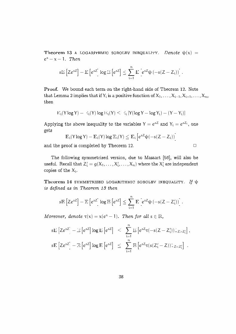
Theorem 13 a logarithmic sobolev inequality. Denote ψ(x) =
ex − x− 1. Then
sEhZesZ
i−E
hesZ
ilogE
hesZ
i�
n∑i=1
E
hesZψ (−s(Z− Zi))
i.
Proof. We bound each term on the right-hand side of Theorem 12. Note
that Lemma 2 implies that if Yi is a positive function of X1, . . . , Xi−1, Xi+1, . . . , Xn,
then
Ei(Y log Y) −Ei(Y) logEi(Y) � Ei [Y(log Y − log Yi) − (Y − Yi)]
Applying the above inequality to the variables Y = esZ and Yi = esZi, one
gets
Ei(Y log Y) −Ei(Y) logEi(Y) � Ei
hesZψ(−s(Z− Zi))
iand the proof is completed by Theorem 12. 2
The following symmetrized version, due to Massart [56], will also be
useful. Recall that Z 0i = g(X1, . . . , X0i, . . . , Xn) where the X 0i are independent
copies of the Xi.
Theorem 14 symmetrized logarithmic sobolev inequality. If ψ
is de�ned as in Theorem 13 then
sEhZesZ
i−E
hesZ
ilogE
hesZ
i�
n∑i=1
E
hesZψ (−s(Z− Z 0i))
i.
Moreover, denote τ(x) = x(ex − 1). Then for all s 2 R,
sEhZesZ
i−E
hesZ
ilogE
hesZ
i�
n∑i=1
E
hesZτ(−s(Z− Z 0i))1Z>Z 0
i
i,
sEhZesZ
i−E
hesZ
ilogE
hesZ
i�
n∑i=1
E
hesZτ(s(Z 0i − Z))1Z<Z 0
i
i.
38

Proof. The �rst inequality is proved exactly as Theorem 13, just by noting
that, just like Zi, Z0i is also independent of Xi. To prove the second and
third inequalities, write
esZψ (−s(Z− Z 0i)) = esZψ (−s(Z− Z 0i))1Z>Z 0
i+ esZψ (s(Z 0i − Z))1Z<Z 0
i.
By symmetry, the conditional expectation of the second term may be writ-
ten as
Ei
hesZψ (s(Z 0i − Z))1Z<Z 0
i
i= Ei
hesZ 0
iψ (s(Z− Z 0i))1Z>Z 0
i
i= Ei
hesZe−s(Z−Z 0
i)ψ (s(Z− Z 0i))1Z>Z 0
i
i.
Summarizing, we have
Ei
hesZψ (−s(Z− Z 0i))
i= Ei
h�ψ (−s(Z− Z 0i)) + e−s(Z−Z 0
i)ψ (s(Z− Z 0i))�esZ1Z>Z 0
i
i.
The second inequality of the theorem follows simply by noting that ψ(x)+
exψ(−x) = x(ex − 1) = τ(x). The last inequality follows similarly. 2
5.4 First example: bounded di�erences and more
The purpose of this section is to illustrate how the logarithmic Sobolev
inequalities shown in the previous section may be used to obtain powerful
exponential concentration inequalities. The �rst result is rather easy to
obtain, yet it turns out to be very useful. Also, its proof is prototypical in
the sense that it shows, in a transparent way, the main ideas.
Theorem 15 Assume that there exists a positive constant C such that,
almost surely,n∑
i=1
(Z− Z 0i)21Z>Z 0
i� C .
Then for all t > 0,
P [Z−EZ > t] � e−t2/4C .
39
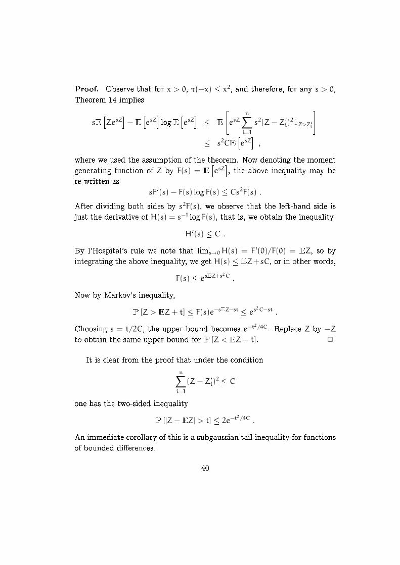
Proof. Observe that for x > 0, τ(−x) � x2, and therefore, for any s > 0,
Theorem 14 implies
sEhZesZ
i−E
hesZ
ilogE
hesZ
i� E
24esZn∑
i=1
s2(Z− Z 0i)21Z>Z 0
i
35� s2CE
hesZ
i,
where we used the assumption of the theorem. Now denoting the moment
generating function of Z by F(s) = E
hesZ
i, the above inequality may be
re-written as
sF 0(s) − F(s) log F(s) � Cs2F(s) .After dividing both sides by s2F(s), we observe that the left-hand side is
just the derivative of H(s) = s−1 log F(s), that is, we obtain the inequality
H 0(s) � C .By l'Hospital's rule we note that lims→0H(s) = F 0(0)/F(0) = EZ, so by
integrating the above inequality, we get H(s) � EZ+sC, or in other words,
F(s) � esEZ+s2C .
Now by Markov's inequality,
P [Z > EZ+ t] � F(s)e−sEZ−st � es2C−st .
Choosing s = t/2C, the upper bound becomes e−t2/4C. Replace Z by −Z
to obtain the same upper bound for P [Z < EZ− t]. 2
It is clear from the proof that under the condition
n∑i=1
(Z− Z 0i)2 � C
one has the two-sided inequality
P [|Z−EZ| > t] � 2e−t2/4C .
An immediate corollary of this is a subgaussian tail inequality for functions
of bounded di�erences.
40
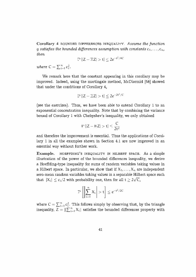
Corollary 4 bounded differences inequality. Assume the function
g satis�es the bounded di�erences assumption with constants c1, . . . , cn,
then
P [|Z−EZ| > t] � 2e−t2/4C
where C =∑n
i=1 c2i .
We remark here that the constant appearing in this corollary may be
improved. Indeed, using the martingale method, McDiarmid [58] showed
that under the conditions of Corollary 4,
P [|Z−EZ| > t] � 2e−2t2/C
(see the exercises). Thus, we have been able to extend Corollary 1 to an
exponential concentration inequality. Note that by combining the variance
bound of Corollary 1 with Chebyshev's inequality, we only obtained
P [|Z−EZ| > t] � C
2t2
and therefore the improvement is essential. Thus the applications of Corol-
lary 1 in all the examples shown in Section 4.1 are now improved in an
essential way without further work.
Example. hoeffding's inequality in hilbert space. As a simple
illustration of the power of the bounded di�erences inequality, we derive
a Hoe�ding-type inequality for sums of random variables taking values in
a Hilbert space. In particular, we show that if X1, . . . , Xn are independent
zero-mean random variables taking values in a separable Hilbert space such
that kXik � ci/2 with probability one, then for all t � 2pC,
P
24 n∑
i=1
Xi
> t35 � e−t2/2C
where C =∑n
i=1 c2i . This follows simply by observing that, by the triangle
inequality, Z = k∑ni=1 Xik satis�es the bounded di�erences property with
41

constants ci, and therefore
P
24 n∑
i=1
Xi
> t35 = P
24 n∑
i=1
Xi
−E
n∑
i=1
Xi
> t−E
n∑
i=1
Xi
35
� exp
0@−2 (t−E k∑n
i=1 Xik)2
C
1A .
The proof is completed by observing that, by independence,
E
n∑
i=1
Xi
�vuuutE
n∑
i=1
Xi
2
=
vuuut n∑i=1
E kXik2 � C .
However, Theorem 15 is much stronger than Corollary 4. To understand
why, just observe that the conditions of Theorem 15 do not require that g
has bounded di�erences. All that's required is that
supx1,...,xn,
x 0
1,...,x 0
n2X
n∑i=1
|g(x1, . . . , xn) − g(x1, . . . , xi−1, x0i, xi+1, . . . , xn)|2 �
n∑i=1
c2i ,
an obviously much milder requirement. The next application is a good
example in which the bounded di�erences inequality does not work, yet
Theorem 15 gives a sharp bound.
Example. the largest eigenvalue of a random symmetric matrix.
Here we derive, using Theorem 15, a result of Alon, Krivelevich, and Vu
[2]. Let A be a symmetric real matrix whose entries Xi,j, 1 � i � j � n are
independent random variables with absolute value bounded by 1. If Z = λ1
is the largest eigenvalue of A, then
P [Z > EZ+ t] � e−t2/16 .
The property of the largest eigenvalue we need is that if v = (v1, . . . , vn) 2R
n is an eigenvector corresponding to the largest eigenvalue λ1 with kvk =
1, then
λ1 = vTAv = supu:kuk=1
uTAu .
42
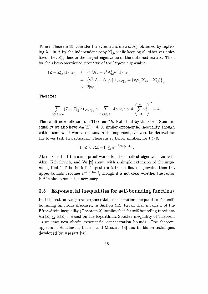
To use Theorem 15, consider the symmetric matrix A 0i,j obtained by replac-
ing Xi,j in A by the independent copy X 0i,j, while keeping all other variables
�xed. Let Z 0i,j denote the largest eigenvalue of the obtained matrix. Then
by the above-mentioned property of the largest eigenvalue,
(Z− Z 0i,j)1Z>Z 0
i,j�
�vTAv− vTA 0
i,jv�1Z>Z 0
i,j
=�vT (A−A 0
i,jv�1Z>Z 0
i,j=�vivj(Xi,j − X 0i,j)
�+
� 2|vivj| .
Therefore,
∑1�i�j�n
(Z− Z 0i,j)21Z>Z 0
i,j�
∑1�i�j�n
4|vivj|2 � 4
0@ n∑i=1
v2i
1A2
= 4 .
The result now follows from Theorem 15. Note that by the Efron-Stein in-
equality we also have Var(Z) � 4. A similar exponential inequality, though
with a somewhat worst constant in the exponent, can also be derived for
the lower tail. In particular, Theorem 20 below implies, for t > 0,
P [Z < EZ− t] � e−t2/16(e−1) .
Also notice that the same proof works for the smallest eigenvalue as well.
Alon, Krivelevich, and Vu [2] show, with a simple extension of the argu-
ment, that if Z is the k-th largest (or k-th smallest) eigenvalue then the
upper bounds becomes e−t2/(16k2), though it is not clear whether the factor
k−2 in the exponent is necessary.
5.5 Exponential inequalities for self-bounding functions
In this section we prove exponential concentration inequalities for self-
bounding functions discussed in Section 4.2. Recall that a variant of the
Efron-Stein inequality (Theorem 2) implies that for self-bounding functions
Var(Z) � E(Z) . Based on the logarithmic Sobolev inequality of Theorem
13 we may now obtain exponential concentration bounds. The theorem
appears in Boucheron, Lugosi, and Massart [14] and builds on techniques
developed by Massart [56].
43
Recall the de�nition of following two functions that we have already
seen in Bennett's inequality and in the logarithmic Sobolev inequalities
above:
h (u) = (1+ u) log (1+ u) − u (u � −1),
and ψ(v) = supu�−1
[uv− h(u)] = ev − v− 1 .
Theorem 16 Assume that g satis�es the self-bounding property. Then
for every s 2 R,logE
hes(Z−EZ)
i� EZψ(s) .
Moreover, for every t > 0,
P [Z � EZ+ t] � exp�−EZh
�t
EZ
��and for every 0 < t � EZ,
P [Z � EZ− t] � exp�−EZh
�−t
EZ
��By recalling that h(u) � u2/(2+2u/3) for u � 0 (we have already used
this in the proof of Bernstein's inequality) and observing that h(u) � u2/2
for u � 0, we obtain the following immediate corollaries: for every t > 0,
P [Z � EZ+ t] � exp
"−
t2
2EZ+ 2t/3
#
and for every 0 < t � EZ,
P [Z � EZ− t] � exp
"−t2
2EZ
#.
Proof. We apply Lemma 13. Since the function ψ is convex with ψ (0) =
0, for any s and any u 2 [0, 1] , ψ(−su) � uψ(−s). Thus, since Z −
Zi 2 [0, 1], we have that for every s, ψ(−s (Z− Zi)) � (Z− Zi)ψ(−s) and
therefore, Lemma 13 and the condition∑n
i=1(Z− Zi) � Z implies that
sEhZesZ
i−E
hesZ
ilogE
hesZ
i� E
24ψ(−s)esZn∑
i=1
(Z− Zi)
35� ψ(−s)E
hZesZ
i.
44

Introduce eZ = Z − E [Z] and de�ne, for any s, �F(s) = E
heseZi. Then the
inequality above becomes
[s−ψ(−s)]�F0(s)�F(s)
− log �F(s) � EZψ(−s) ,
which, writing G(s) = log F(s), implies
(1− e−s)G0 (s) −G (s) � EZψ (−s) .
Now observe that the function G0 = EZψ is a solution of the ordinary
di�erential equation (1− e−s)G0 (s)−G (s) = EZψ (−s). We want to show
that G � G0. In fact, if G1 = G−G0, then
(1− e−s)G01 (s) −G1 (s) � 0. (3)
Hence, de�ning �G(s) = G1 (s) /(es − 1), we have
(1− e−s) (es − 1) �G0(s) � 0.Hence �G0 is non-positive and therefore �G is non-increasing. Now, since eZ is
centered G01 (0) = 0. Using the fact that s(es−1)−1 tends to 1 as s goes to 0,
we conclude that �G(s) tends to 0 as s goes to 0. This shows that �G is non-
positive on (0,∞) and non-negative over (−∞, 0), hence G1 is everywhere
non-positive, therefore G � G0 and we have proved the �rst inequality of
the theorem. The proof of inequalities for the tail probabilities may be
completed by Cherno�'s bounding:
P [Z−E [Z] � t] � exp
"− sup
s>0(ts−EZψ (s))
#and
P [Z−E [Z] � −t] � exp
"− sup
s<0(−ts−EZψ (s))
#.
The proof is now completed by using the easy-to-check (and well-known)
relations
sups>0
[ts−EZψ (s)] = EZh (t/EZ) for t > 0
sups<0
[−ts−EZψ(s)] = EZh(−t/EZ) for 0 < t � EZ.2
45
5.6 Combinatorial entropies
Theorems 2 and 16 provide concentration inequalities for functions having
the self-bounding property. In Section 4.2 several examples of such func-
tions are discussed. The purpose of this section is to show a whole new
class of self-bounding functions that we call combinatorial entropies.
Example. vc entropy. In this �rst example we consider the so-called
Vapnik-Chervonenkis (or vc) entropy, a quantity closely related to the vc
dimension discussed in Section 4.2. Let A be an arbitrary collection of
subsets of X , and let xn1 = (x1, . . . , xn) be a vector of n points of X . Recall
that the shatter coe�cient is de�ned as the size of the trace of A on xn1 ,
that is,
T(xn1 ) = |tr(xn
1 )| = |{A \ {x1, . . . , xn} : A 2 A}| .
The vc entropy is de�ned as the logarithm of the shatter coe�cient, that
is,
h(xn1 ) = log2 T(x
n1 ) .
Lemma 3 The vc entropy has the self-bounding property.
Proof. We need to show that there exists a function h 0 of n− 1 variables
such that for all i = 1, . . . , n, writing x(i) = (x1, . . . , xi−1, xi+1, . . . , xn),
0 � h(xn1 ) − h 0(x(i)) � 1 and
n∑i=1
�h(xn
1 ) − h 0(x(i))�� h(xn
1 ).
We de�ne h 0 the natural way, that is, as the entropy based on the n − 1
points in its arguments. Then clearly, for any i, h 0(x(i)) � h(xn1 ), and the
di�erence cannot be more than one. The nontrivial part of the proof is
to show the second property. We do this using Han's inequality (Theorem
10).
Consider the uniform distribution over the set tr(xn1 ). This de�nes a
random vector Y = (Y1, . . . , Yn) 2 Yn. Then clearly,
h(xn1 ) = log2 |tr(xn
1 )(x)| =1
ln 2H(Y1, . . . , Yn)
46
where H(Y1, . . . , Yn) is the (joint) entropy of Y1, . . . , Yn. Since the uniform
distribution maximizes the entropy, we also have, for all i � n, that
h 0(x(i)) � 1
ln 2H(Y1, . . . , Yi−1, Yi+1, . . . , Yn).
Since by Han's inequality
H(Y1, . . . , Yn) � 1
n− 1
n∑i=1
H(Y1, . . . , Yi−1, Yi+1, . . . , Yn)|,
we haven∑
i=1
�h(xn
1 ) − h 0(x(i))�� h(xn
1 )
as desired. 2
The above lemma, together with Theorems 2 and 15 immediately imply
the following:
Corollary 5 Let X1, . . . , Xn be independent random variables taking their
values in X and let Z = h(Xn1 ) denote the random vc entropy. Then
Var(Z) � E[Z], for t > 0
P [Z � EZ+ t] � exp
"−
t2
2EZ+ 2t/3
#,
and for every 0 < t � EZ,
P [Z � EZ− t] � exp
"−t2
2EZ
#.
Moreover, for the random shatter coe�cient T(Xn1 ), we have
E log2 T(Xn1 ) � log2ET(X
n1 ) � log2 eE log2 T(X
n1 ) .
Note that the left-hand side of the last statement follows from Jensen's
inequality, while the right-hand side by taking s = ln 2 in the �rst inequality
of Theorem 16. This last statement shows that the expected vc entropy
E log2 T(Xn1 ) and the annealed vc entropy are tightly connected, regardless
47
of the class of sets A and the distribution of the Xi's. We note here that
this fact answers, in a positive way, an open question raised by Vapnik [79,
pages 53�54]: the empirical risk minimization procedure is non-trivially
consistent and rapidly convergent if and only if the annealed entropy rate
(1/n) log2E[T(X)] converges to zero. For the de�nitions and discussion we
refer to [79].
The proof of concentration of the vc entropy may be generalized, in a
straightforward way, to a class of functions we call combinatorial entropies
de�ned as follows.
Let xn1 = (x1, . . . , xn) be an n-vector of elements with xi 2 Xi to which
we associate a set tr(xn1 ) � Yn of n-vectors whose components are elements
of a possibly di�erent set Y. We assume that for each x 2 X n and i � n, theset tr(x(i)) = tr(x1, . . . , xi−1, xi+1, . . . , xn) is the projection of tr(xn
1 ) along
the ith coordinate, that is,
tr(x(i)) ={y(i) = (y1, . . . , yi−1, yi+1, . . . , yn) 2 Yn−1 :
9yi 2 Y such that (y1, . . . , yn) 2 tr(xn1 )
}.
The associated combinatorial entropy is h(xn1 ) = logb |tr(xn
1 )| where b is an
arbitrary positive number.
Just like in the case of vc entropy, combinatorial entropies may be
shown to have the self-bounding property. (The details are left as an exer-
cise.) Then we immediately obtain the following generalization:
Theorem 17 Assume that h(xn1 ) = logb |tr(xn
1 )| is a combinatorial en-
tropy such that for all x 2 X n and i � n,h(xn
1 ) − h(x(i)) � 1 .If Xn
1 = (X1, . . . , Xn) is a vector of n independent random variables
taking values in X , then the random combinatorial entropy Z = h(Xn1 )
satis�es
P [Z � E [Z] + t] � exp
"−
t2
2E[Z] + 2t/3
#,
and
P [Z � E [Z] − t] � exp
"−
t2
2E[Z]
#.
48
Moreover,
E [logb |tr(Xn1 )|] � logbE[|tr(Xn
1 )|] � b− 1
log bE [logb |tr(Xn
1 )|] .
Example. increasing subsequences. Recall the setup of the example of
increasing subsequences of Section 4.2, and let N(xn1 ) denote the number
of di�erent increasing subsequences of xn1 . Observe that log2N(xn
1 ) is a
combinatorial entropy. This is easy to see by considering Y = {0, 1}, and
by assigning, to each increasing subsequence i1 < i2 < � � � < im of xn1 , a
binary n-vector yn1 = (y1, . . . , yn) such that yj = 1 if and only if j = ik for
some k = 1, . . . ,m (i.e., the indices appearing in the increasing sequence
are marked by 1). Now the conditions of Theorem 17 are obviously met,
and therefore Z = log2N(Xn1 ) satis�es all three inequalities of Theorem 17.
This result signi�cantly improves a concentration inequality obtained by
Frieze [33] for log2N(Xn1 ).
5.7 Variations on the theme
In this section we show how the techniques of the entropy method for
proving concentration inequalities may be used in various situations not
considered so far. The versions di�er in the assumptions on how∑n
i=1(Z−
Z 0i)2 is controlled by di�erent functions of Z. For various other versions
with applications we refer to Boucheron, Lugosi, and Massart [15]. In
all cases the upper bound is roughly of the form e−t2/σ2where σ2 is the
corresponding Efron-Stein upper bound on Var(Z). The �rst inequality may
be regarded as a generalization of the upper tail inequality in Theorem 16.
Theorem 18 Assume that there exist positive constants a and b such
thatn∑
i=1
(Z− Z 0i)21Z>Z 0
i� aZ+ b .
Then for s 2 (0, 1/a),
logE[exp(s(Z−E[Z]))] � s2
1− as(aEZ+ b)
49
and for all t > 0,
P {Z > EZ+ t} � exp
−t2
4aEZ+ 4b+ 2at
!.
Proof. Let s > 0. Just like in the �rst steps of the proof of Theorem 15,
we use the fact that for x > 0, τ(−x) � x2, and therefore, by Theorem 14
we have
sEhZesZ
i−E
hesZ
ilogE
hesZ
i� E
24esZn∑
i=1
(Z− Z 0i)21Z>Z 0
i
35� s2
�aE
hZesZ
i+ bE
hesZ
i�,
where at the last step we used the assumption of theorem.
Denoting, once again, F(s) = EhesZ
i, the above inequality becomes
sF 0(s) − F(s) log F(s) � as2F 0(s) + bs2F(s) .
After dividing both sides by s2F(s), once again we see that the left-hand
side is just the derivative of H(s) = s−1 log F(s), so we obtain
H 0(s) � a(log F(s)) 0 + b .
Using the fact that lims→0H(s) = F 0(0)/F(0) = EZ and log F(0) = 0, and
integrating the inequality, we obtain
H(s) � EZ+ a log F(s) + bs ,
or, if s < 1/a,
logE[exp(s(Z−E[Z]))] � s2
1− as(aEZ+ b) ,
proving the �rst inequality. The inequality for the upper tail now follows
by Markov's inequality and Exercise 17. 2
There is a subtle di�erence between upper and lower tail bounds. Bounds
for the lower tail P {Z < EZ− t} may be easily derived, due to the as-
sociation inequality of Theorem 2, under much more general conditions
on∑n
i=1(Z − Z 0i)21Z<Z 0
i(note the di�erence between this quantity and∑n
i=1(Z− Z 0i)21Z>Z 0
iappearing in the theorem above!).
50
Theorem 19 Assume that for some nondecreasing function g,
n∑i=1
(Z− Z 0i)21Z<Z 0
i� g(Z) .
Then for all t > 0,
P [Z < EZ− t] � exp
−t2
4E[g(Z)]
!.
Proof. To prove lower-tail inequalities we obtain upper bounds for F(s) =
E[exp(sZ)] with s < 0. By the third inequality of Theorem 14,
sEhZesZ
i−E
hesZ
ilogE
hesZ
i�
n∑i=1
E
hesZτ(s(Z 0i − Z))1Z<Z 0
i
i
�n∑
i=1
E
hesZs2(Z 0i − Z)2
1Z<Z 0
i
i(using s < 0 and that τ(−x) � x2 for x > 0)
= s2E
24esZn∑
i=1
(Z− Z 0i)21Z<Z 0
i
35� s2E
hesZg(Z)
i.
Since g(Z) is a nondecreasing and esZ is a decreasing function of Z, Cheby-
shev's association inequality (Theorem 2) implies that
E
hesZg(Z)
i� E
hesZ
iE[g(Z)] .
Thus, dividing both sides of the obtained inequality by s2F(s) and writing
H(s) = (1/s) log F(s), we obtain
H 0(s) � E[g(Z)] .
integrating the inequality in the interval [s, 0) we obtain
F(s) � exp(s2E[g(Z)] + sE[Z]) .
51
Markov's inequality and optimizing in s now implies the theorem. 2
The next result is useful when one in interested in lower-tail bounds but∑ni=1(Z−Z 0i)
21Z<Z 0
iis di�cult to handle. In some cases
∑ni=1(Z−Z 0i)
21Z>Z 0
i
is easier to bound. In such a situation we need the additional guarantee
that |Z−Z 0i| remains bounded. Without loss of generality, we assume that
the bound is 1.
Theorem 20 Assume that there exists a nondecreasing function g such
that∑n
i=1(Z−Z 0i)21Z>Z 0
i� g(Z) and for any value of Xn
1 and Xi0, |Z−Z 0i| �
1. Then for all K > 0, s 2 [0, 1/K)
logEhexp(−s(Z−E[Z]))
i� s2τ(K)
K2E[g(Z)] ,
and for all t > 0, with t � (e− 1)E[g(Z)] we have
P [Z < EZ− t] � exp
−
t2
4(e− 1)E[g(Z)]
!.
Proof. The key observation is that the function τ(x)/x2 = (ex − 1)/x is
increasing if x > 0. Choose K > 0. Thus, for s 2 (−1/K, 0), the second
inequality of Theorem 14 implies that
sEhZesZ
i−E
hesZ
ilogE
hesZ
i�
n∑i=1
E
hesZτ(−s(Z− Z(i)))1Z>Z 0
i
i
� s2τ(K)
K2E
24esZn∑
i=1
(Z− Z(i))21Z>Z 0
i
35� s2
τ(K)
K2E
hg(Z)esZ
i,
where at the last step we used the assumption of the theorem.
Just like in the proof of Theorem 19, we boundEhg(Z)esZ
ibyE[g(Z)]E
hesZ
i.
The rest of the proof is identical to that of Theorem 19. Here we took K = 1.
2
52
Exercises
Exercise 15 Relax the condition of Theorem 15 in the following way. Show
that if
E
24 n∑i=1
(Z− Z 0i)21Z>Z 0
i
����Xn1
35 � cthen for all t > 0,
P [Z > EZ+ t] � e−t2/4c
and if
E
24 n∑i=1
(Z− Z 0i)21Z 0
i>Z
����Xn1
35 � c ,then
P [Z < EZ− t] � e−t2/4c .
Exercise 16 mcdiarmid's bounded differences inequality. Prove
that under the conditions of Corollary 4, the following improvement holds:
P [|Z−EZ| > t] � 2e−2t2/C
(McDiarmid [58]). Hint: Write Z as a sum of martingale di�erences as in
the proof of Theorem 7. Use Cherno�'s bounding and proceed as in the
proof of Hoe�ding's inequality, noting that the argument works for sums
of martingale di�erences.
Exercise 17 Let C and a denote two positive real numbers and denote
h1(x) = 1+ x−p1+ 2x. Show that
supλ2[0,1/a)
λt−
Cλ2
1− aλ
!=2C
a2h1
�at
2C
�� t2
2�2C+ at
�and that the supremum is attained at
λ =1
a
1−
�1+
at
C
�−1/2!.
Also,
supλ2[0,∞)
λt−
Cλ2
1+ aλ
!=2C
a2h1
�−at
2C
�� t2
4C
53

if t < C/a and the supremum is attained at
λ =1
a
�1−
at
C
�−1/2
− 1
!.
Exercise 18 Assume that h(xn1 ) = logb|tr(x)| is a combinatorial entropy
such that for all x 2 X n and i � n,
h(xn1 ) − h(x(i)) � 1
Show that h has the self-bounding property.
Exercise 19 Assume that Z = g(Xn1 ) = g(X1, . . . , Xn) where X1, . . . , Xn are
independent real-valued random variables and g is a nondecreasing function
of each variable. Suppose that there exists another nondecreasing function
f : Rn → R such that
n∑i=1
(Z− Z 0i)21Z<Z 0
i� f(Xn
1 ) .
Show that for all t > 0,
P[Z < EZ− t] � e−t2/(4Ef(Xn1 ))
54
6 Concentration of measure
In this section we address the �isoperimetric� approach to concentration in-
equalities, promoted and developed, in large part, by Talagrand [75, 76, 77].
First we give an equivalent formulation of the bounded di�erences inequal-
ity (Corollary 4) which shows that any not too small set in a product prob-
ability space has the property that the probability of those points whose
Hamming distance from the set is much larger thanpn is exponentially
small. Then, using the full power of Theorem 15, we provide a signi�cant
improvement of this concentration-of-measure result, known as Talagrand's
convex distance inequality.
6.1 Bounded di�erences inequality revisited
Consider independent random variables X1, . . . , Xn taking their values in
a (measurable) set X and denote the vector of these variables by Xn1 =
(X1, . . . , Xn) taking its value in X n.
Let A � X n be an arbitrary (measurable) set and write P[A] = P[Xn1 2
A]. The Hamming distance d(xn1 , y
n1 ) between the vectors xn
1 , yn1 2 X n is
de�ned as the number of coordinates in which xn1 and yn
1 di�er. Introduce
d(xn1 , A) = min
yn12A
d(xn1 , y
n1 ),
the Hamming distance between the set A and the point xn1 . The basic
result is the following:
Theorem 21 For any t > 0,
P
"d(Xn
1 , A) � t+
sn
2log
1
P[A]
#� e−2t2/n .
Observe that on the right-hand side we have the measure of the com-
plement of the t-blowup of the set A, that is, the measure of the set of
points whose Hamming distance from A is at least t. If we consider a set,
say, with P[A] = 1/106, we see something very surprising: the measure
of the set of points whose Hamming distance to A is more than 10pn is
55
smaller than e−108! In other words, product measures are concentrated on
extremely small sets�hence the name �concentration of measure�.
Proof. Observe that the function g(xn1 ) = d(xn
1 , A) cannot change by more
than 1 by altering one component of xn1 , that is, it has the bounded di�er-
ences property with constants c1 = � � � = cn = 1. Thus, by the bounded
di�erences inequality (Theorem 4 with the optimal constants given in Ex-
ercise 16),
P[Ed(Xn1 , A) − d(Xn
1 , A) � t] � e−2t2/n.
But by taking t = Ed(Xn1 , A), the left-hand side becomes P[d(Xn
1 , A) �0] = P[A], so the above inequality implies
E[d(Xn1 , A)] �
sn
2log
1
P[A].
Then, by using the bounded di�erences inequality again, we obtain
P
"d(Xn
1 , A) � t+
sn
2log
1
P{A}
#� e−2t2/n
as desired. 2
Observe that the bounded di�erences inequality may also be derived
from the above theorem. Indeed, if we consider a function g on X n having
the bounded di�erences property with constants ci = 1 (for simplicity),
then we may let A = {xn1 2 X n : g(xn
1 ) � M[Z]}, where M[Z] denotes a
median of the random variable Z = g(X1, . . . , Xn). Then clearly P[A] �1/2, so the above theorem implies
P[Z−MZ � t+
sn
2log 2] � e−2t2/n .
This has the same form as the bounded di�erences inequality except that
the expected value of Z is replaced by its median. This di�erence is usually
negligible, since
|EZ−MZ| � E|Z−MZ| =
∫∞0
P[|Z−MZ| � t]dt,
so whenever the deviation of Z from its mean is small, its expected value
must be close to its median (see Exercise 20).
56
6.2 Convex distance inequality
In a remarkable series of papers (see [77],[75],[76]), Talagrand developed an
induction method to prove powerful concentration results in many cases
when the bounded di�erences inequality fails. Perhaps the most widely
used of these is the so-called �convex-distance inequality�, see also Steele
[74], McDiarmid [59] for surveys with several interesting applications. Here
we use Theorem 15 to derive a version of the convex distance inequality.
For several extensions and variations we refer to Talagrand [77],[75],[76].
To understand Talagrand's inequality, we borrow a simple argument
from [59]. First observe that Theorem 21 may be easily generalized by
allowing the distance of the point Xn1 from the set A to be measured by a
weighted Hamming distance
dα(xn1 , A) = inf
yn12A
dα(xn1 , y
n1 ) = inf
yn12A
∑i:xi 6=yi
|αi|
where α = (α1, . . . , αn) is a vector of nonnegative numbers. Repeating the
argument of the proof of Theorem 21, we obtain, for all α,
P
24dα(Xn1 , A) � t+
vuutkαk2
2log
1
P[A]
35 � e−2t2/kαk2
,
where kαk =q∑n
i=1 α2i denotes the euclidean norm of α. Thus, for exam-
ple, for all vectors α with unit norm kαk = 1,
P
"dα(Xn
1 , A) � t+
s1
2log
1
P[A]
#� e−2t2
.
Thus, denoting u =q
12log 1
P[A], for any t � u,
P [dα(Xn1 , A) � t] � e−2(t−u)2
.
On the one hand, if t �q
−2 logP[A], then P[A] � e−t2/2. On the other
hand, since (t−u)2 � t2/4 for t � 2u, for any t �q2 log 1
P[A]the inequality
above implies P [dα(Xn1 , A) � t] � e−t2/2 . Thus, for all t > 0, we have
supα:kαk=1
P[A]�P [dα(Xn1 , A) � t] � sup
α:kαk=1min (P[A],P [dα(Xn
1 , A) � t]) � e−t2/2 .
57

The main message of Talagrand's inequality is that the above inequality
remains true even if the supremum is taken within the probability. To
make this statement precise, introduce, for any xn1 = (x1, . . . , xn) 2 X n, the
convex distance of xn1 from the set A by
dT (xn1 , A) = sup
α2[0,∞)n:kαk=1
dα(xn1 , A) .
The next result is a prototypical result from Talagrand's important paper
[75]. For an even stronger concentration-of-measure result we refer to [76].
Theorem 22 convex distance inequality. For any subset A � X n
with P[Xn1 2 A] � 1/2 and t > 0,
min (P[A],P [dT (Xn1 , A) � t]) � e−t2/4 .
Even though at the �rst sight it is not obvious how Talagrand's result
can be used to prove concentration for general functions g of Xn1 , appar-
ently with relatively little work, the theorem may be converted into very
useful inequalities. Talagrand [75], Steele [74], and McDiarmid [59] survey
a large variety of applications. Instead of reproducing Talagrand's original
proof here we show how Theorem 15 and 20 imply the convex distance in-
equality. (This proof gives a slightly worse exponent than the one obtained
by Talagrand's method stated above.)
Proof. De�ne the random variable Z = dT (Xn1 , A). First we observe that
dT (xn1 , A) can be represented as a saddle point. Let M(A) denote the set
of probability measure on A. Then
dT (xn1 , A) = sup
α:kαk�1inf
ν2M(A)
∑j
αjEν[1xj 6=Yj]
(where Yn1 is distributed according to ν)
= infν2M(A)
supα:kαk�1
∑j
αjEν[1xj 6=Yj]
where the saddle point is achieved. This follows from Sion's minmax The-
orem [71] which states that if f(x, y) denotes a function from X � Y to R
that is convex and lower-semi-continuous with respect to x, concave and
58
upper-semi-continuous with respect to y, where X is convex and compact,
then
infxsup
yf(x, y) = sup
yinfxf(x, y) .
(We omit the details of checking the conditions of Sion's theorem, see [15].)
Let now (bν, bα) be a saddle point for xn1 . We have
Z 0i = infν2M(A)
supα
∑j
αjEν[1x
(i)j 6=Yj
] � infν2M(A)
∑j
bαjEν[1x
(i)j 6=Yj
]
where x(i)j = xj if j 6= i and x
(i)i = x 0i. Let �ν denote the distribution on A
that achieves the in�mum in the latter expression. Now we have
Z = infν
∑j
bαjEν[1xj 6=Yj] �
∑j
bαjE�ν[1xj 6=Yj] .
Hence we get
Z− Z 0i �∑
j
bαjE�ν[1xj 6=Yj− 1
x(i)j 6=Yj
] = bαiE�ν[1xi 6=Yi− 1
x(i)i 6=Yi
] � bαi .
Therefore∑n
i=1(Z − Z 0i)21Z>Z 0
i� ∑
ibα2
i = 1. Thus by Theorem 15 (more
precisely, by its generalization in Exercise 15), for any t > 0,
P [dT (Xn1 , A) −EdT (Xn
1 , A) � t] � e−t2/4.
Similarly, by Theorem 20 we get
P [dT (Xn1 , A) −EdT (Xn
1 , A) � −t] � e−t2/(4(e−1))
which, by taking t = EdT (Xn1 , A), implies
EdT (Xn1 , A) �
s4(e− 1) log
1
P[A].
P
"dT (Xn
1 , A) −
s4(e− 1) log
1
P[A]� t
#� e−t2/4 .
59
Now if 0 < u �q
−4 logP[A] then P[A] � e−u2/4. On the other hand, if
u �q
−4 logP[A] then
P [dT (Xn1 , A) > u] � P
24dT (Xn1 , A) −
s4(e− 1) log
1
P[A]> u− u
se− 1
e
35
� exp
−u2�1−
q(e− 1)/e
�2
4
where the second inequality follows from the upper-tail inequality above.
In conclusion, for all u > 0, we have
min (P[A],P [dT (Xn1 , A) � u]) � exp
−u2�1−
q(e− 1)/e
�2
4
which concludes the proof of the convex distance inequality (with a worse
constant in the exponent). 2
6.3 Examples
In what follows we describe an application of the convex distance inequality
for the bin packing discussed in Section 4.1, appearing in Talagrand [75].
Let g(xn1 ) denote the minimum number of bins of size 1 into which the
numbers x1, . . . , xn 2 [0, 1] can be packed. We consider the random variable
Z = g(Xn1 ) where X1, . . . , Xn are independent, taking values in [0, 1].
Corollary 6 Denote Σ =qE
∑ni=1 X
2i . Then for each t > 0,
P[|Z−MZ| � t+ 1] � 8e−t2/(16(2Σ2+t)) .
Proof. First observe (and this is the only speci�c property of g we use in
the proof!) that for any xn1 , y
n1 2 [0, 1]n,
g(xn1 ) � g(yn
1 ) + 2∑
i:xi 6=yi
xi + 1 .
60
To see this it su�ces to show that the xi for which xi 6= yi can be packed
into at mostj2
∑i:xi 6=yi
xi
k+ 1 bins. For this it enough to �nd a packing
such that at most one bin is less than half full. But such a packing must
exist because we can always pack the contents of two half-empty bins into
one.
Denoting by α = α(xn1 ) 2 [0,∞)n the unit vector xn
1 /kxn1 k, we clearly
have ∑i:xi 6=yi
xi = kxn1 k
∑i:xi 6=yi
αi = kxn1 kdα(xn
1 , yn1 ) .
Let a be a positive number and de�ne the set Aa = {yn1 : g(yn
1 ) � a}. Then,
by the argument above and by the de�nition of the convex distance, for
each xn1 2 [0, 1]n there exists yn
1 2 Aa such that
g(xn1 ) � g(yn
1 ) + 2∑
i:xi 6=yi
xi + 1 � a+ 2kxn1 kdT (xn
1 , Aa) + 1
from which we conclude that for each a > 0, Z � a+ 2kXn1 kdT (Xn
1 , Aa)+ 1.
Thus, writing Σ =qE
∑ni=1 X
2i for any t � 0,
P[Z � a+ 1+ t]
� P
"Z � a+ 1+ t
2kXn1 k
2p2Σ2 + t
#+P
�kXn
1 k �q2Σ2 + t
�
� P
"dT (Xn
1 , Aa) � t
2p2Σ2 + t
#+ e−(3/8)(Σ2+t)
where the bound on the second term follows by a simple application of
Bernstein's inequality, see Exercise 21.
To obtain the desired inequality, we use the obtained bound with two
di�erent choices of a. To derive a bound for the upper tail of Z, we take
a =MZ. Then P[Aa] � 1/2 and the convex distance inequality yields
P[Z �MZ+ 1+ t] � 2�e−t2/(16(2Σ2+t)) + e−(3/8)(Σ2+t)
�� 4e−t2/(16(2Σ2+t)) .
We obtain a similar inequality in the same way for P[Z � MZ − 1 − t] by
taking a =MZ− t− 1. 2
61

Exercises
Exercise 20 Let X be a random variable with medianMX such that there
exist positive constants a and b such that for all t > 0,
P[|X−MX| > t] � ae−t2/b .
Show that |MX−EX| � apbπ/2.
Exercise 21 Let X1, . . . , Xn be independent random variables taking val-
ues is [0, 1]. Show that
P
264vuuut n∑
i=1
X2i �
vuuut2E n∑i=1
X2i + t
375 � e−(3/8)(E∑n
i=1 X2i +t) .
References
[1] R. Ahlswede, P. Gács, and J. Körner. Bounds on conditional prob-
abilities with applications in multi-user communication. Zeitschrift
für Wahrscheinlichkeitstheorie und verwandte Gebiete, 34:157�177,
1976. (correction in 39:353�354,1977).
[2] N. Alon, M. Krivelevich, and V.H. Vu. On the concentration of eigen-
values of random symmetric matrices. Israel Math. Journal, 131:259�
267, 2002.
[3] M. Anthony and P. L. Bartlett. Neural Network Learning: Theoret-
ical Foundations. Cambridge University Press, Cambridge, 1999.
[4] J. Baik, P. Deift, and K. Johansson. On the distribution of the length
of the second row of a Young diagram under Plancherel measure. Ge-
ometric and Functional Analysis, 10:702�731, 2000.
[5] P. Bartlett, S. Boucheron, and G. Lugosi. Model selection and error
estimation. Machine Learning, 48:85�113, 2002.
62
[6] P. Bartlett, O. Bousquet, and S. Mendelson. Localized Rademacher
complexities. In Proceedings of the 15th annual conference on Com-
putational Learning Theory, pages 44�48, 2002.
[7] P.L. Bartlett and S. Mendelson. Rademacher and gaussian complexi-
ties: risk bounds and structural results. Journal of Machine Learn-
ing Research, 3:463�482, 2002.
[8] W. Beckner. A generalized Poincaré inequality for Gaussian measures.
Proceedings of the American Mathematical Society, 105:397�400,
1989.
[9] G. Bennett. Probability inequalities for the sum of independent ran-
dom variables. Journal of the American Statistical Association,
57:33�45, 1962.
[10] S.N. Bernstein. The Theory of Probabilities. Gastehizdat Publishing
House, Moscow, 1946.
[11] A. Blumer, A. Ehrenfeucht, D. Haussler, and M.K. Warmuth. Learn-
ability and the Vapnik-Chervonenkis dimension. Journal of the
ACM, 36:929�965, 1989.
[12] S. Bobkov and M. Ledoux. Poincaré's inequalities and Talagrands's
concentration phenomenon for the exponential distribution. Probabil-
ity Theory and Related Fields, 107:383�400, 1997.
[13] B. Bollobás and G. Brightwell. The height of a random partial order:
Concentration of measure. Annals of Applied Probability, 2:1009�
1018, 1992.
[14] S. Boucheron, G. Lugosi, and P. Massart. A sharp concentration
inequality with applications. Random Structures and Algorithms,
16:277�292, 2000.
[15] S. Boucheron, G. Lugosi, and P. Massart. Concentration inequalities
using the entropy method. The Annals Probability, 31:1583�1614,
2003.
63
[16] O. Bousquet. A Bennett concentration inequality and its application
to suprema of empirical processes. C. R. Acad. Sci. Paris, 334:495�
500, 2002.
[17] O. Bousquet. New approaches to statistical learning theory. Annals
of the Institute of Statistical Mathematics, 2003.
[18] D. Chafaï. On φ-entropies and φ-Sobolev inequalities. Technical re-
port, arXiv.math.PR/0211103, 2002.
[19] H. Cherno�. A measure of asymptotic e�ciency of tests of a hypothesis
based on the sum of observations. Annals of Mathematical Statistics,
23:493�507, 1952.
[20] V. Chvátal and D. Sanko�. Longest common subsequences of two
random sequences. Journal of Applied Probability, 12:306�315, 1975.
[21] T.M. Cover and J.A. Thomas. Elements of Information Theory.
John Wiley, New York, 1991.
[22] V. Dan£ík and M. Paterson. Upper bound for the expected. In Pro-
ceedings of STACS'94. Lecture notes in Computer Science, 775,
pages 669�678. Springer, New York, 1994.
[23] J.P. Deken. Some limit results for longest common subsequences. Dis-
crete Mathematics, 26:17�31, 1979.
[24] A. Dembo. Information inequalities and concentration of measure.
Annals of Probability, 25:927�939, 1997.
[25] L. Devroye. The kernel estimate is relatively stable. Probability The-
ory and Related Fields, 77:521�536, 1988.
[26] L. Devroye. Exponential inequalities in nonparametric estimation. In
G. Roussas, editor, Nonparametric Functional Estimation and Re-
lated Topics, pages 31�44. NATO ASI Series, Kluwer Academic Pub-
lishers, Dordrecht, 1991.
64
[27] L. Devroye and L. Györ�. Nonparametric Density Estimation: The
L1 View. John Wiley, New York, 1985.
[28] L. Devroye, L. Györ�, and G. Lugosi. A Probabilistic Theory of
Pattern Recognition. Springer-Verlag, New York, 1996.
[29] L. Devroye and G. Lugosi. Combinatorial Methods in Density Es-
timation. Springer-Verlag, New York, 2000.
[30] D. Dubdashi and D. Ranjan. Balls and bins: a study in negative de-
pendence. Random Structures and Algorithms, pages 99�124, 1998.
[31] R.M. Dudley. Uniform Central Limit Theorems. Cambridge Uni-
versity Press, Cambridge, 1999.
[32] B. Efron and C. Stein. The jackknife estimate of variance. Annals of
Statistics, 9:586�596, 1981.
[33] A.M. Frieze. On the length of the longest monotone subsequence in
a random permutation. Annals of Applied Probability, 1:301�305,
1991.
[34] P. Groeneboom. Hydrodynamical methods for analyzing longest in-
creasing subsequences. probabilistic methods in combinatorics and
combinatorial optimization. Journal of Computational and Applied
Mathematics, 142:83�105, 2002.
[35] T. Hagerup and C. Rüb. A guided tour of Cherno� bounds. Informa-
tion Processing Letters, 33:305�308, 1990.
[36] G.H. Hall, J.E. Littlewood, and G. Pólya. Inequalities. Cambridge
University Press, London, 1952.
[37] T.S. Han. Nonnegative entropy measures of multivariate symmetric
correlations. Information and Control, 36, 1978.
[38] W. Hoe�ding. Probability inequalities for sums of bounded random
variables. Journal of the American Statistical Association, 58:13�
30, 1963.
65
[39] S. Janson, T. �uczak, and A. Ruci«ski. Random graphs. John Wiley,
New York, 2000.
[40] R.M. Karp. Probabilistic Analysis of Algorithms. Class Notes, Uni-
versity of California, Berkeley, 1988.
[41] V. Koltchinskii. Rademacher penalties and structural risk minimiza-
tion. IEEE Transactions on Information Theory, 47:1902�1914,
2001.
[42] V. Koltchinskii and D. Panchenko. Empirical margin distributions and
bounding the generalization error of combined classi�ers. Annals of
Statistics, 30, 2002.
[43] R. Lataªa and C. Oleszkiewicz. Between Sobolev and Poincaré. In Ge-
ometric Aspects of Functional Analysis, Israel Seminar (GAFA),
1996-2000, pages 147�168. Springer, 2000. Lecture Notes in Mathe-
matics, 1745.
[44] M. Ledoux. Isoperimetry and gaussian analysis. In P. Bernard, editor,
Lectures on Probability Theory and Statistics, pages 165�294. Ecole
d'Eté de Probabilités de St-Flour XXIV-1994, 1996.
[45] M. Ledoux. On Talagrand's deviation inequalities for product
measures. ESAIM: Probability and Statistics, 1:63�87, 1997.
http://www.emath.fr/ps/.
[46] M. Ledoux. Concentration of measure and logarithmic sobolev in-
equalities. In Séminaire de Probabilités XXXIII. Lecture Notes in
Mathematics 1709, pages 120�216. Springer, 1999.
[47] M. Ledoux. The concentration of measure phenomenon. American
Mathematical Society, Providence, RI, 2001.
[48] B.F. Logan and L.A. Shepp. A variational problem for Young tableaux.
Advances in Mathematics, 26:206�222, 1977.
[49] Malwina J. Luczak and Colin McDiarmid. Concentration for locally
acting permutations. Discrete Mathematics, page to appear, 2003.
66
[50] G. Lugosi. Pattern classi�cation and learning theory. In L. Györ�,
editor, Principles of Nonparametric Learning, pages 5�62. Springer,
Wien, 2002.
[51] G. Lugosi and M. Wegkamp. Complexity regularization via localized
random penalties. Annals of Statistics, 32:1679�1697, 2004.
[52] K. Marton. A simple proof of the blowing-up lemma. IEEE Trans-
actions on Information Theory, 32:445�446, 1986.
[53] K. Marton. Bounding d-distance by informational divergence: a way
to prove measure concentration. Annals of Probability, 24:857�866,
1996.
[54] K. Marton. A measure concentration inequality for contracting Markov
chains. Geometric and Functional Analysis, 6:556�571, 1996. Erra-
tum: 7:609�613, 1997.
[55] P. Massart. Optimal constants for Hoe�ding type inequalities. Tech-
nical report, Mathematiques, Université de Paris-Sud, Report 98.86,
1998.
[56] P. Massart. About the constants in Talagrand's concentration inequal-
ities for empirical processes. Annals of Probability, 28:863�884, 2000.
[57] P. Massart. Some applications of concentration inequalities to statis-
tics. Annales de la Faculté des Sciencies de Toulouse, IX:245�303,
2000.
[58] C. McDiarmid. On the method of bounded di�erences. In Surveys
in Combinatorics 1989, pages 148�188. Cambridge University Press,
Cambridge, 1989.
[59] C. McDiarmid. Concentration. In M. Habib, C. McDiarmid,
J. Ramirez-Alfonsin, and B. Reed, editors, Probabilistic Methods for
Algorithmic Discrete Mathematics, pages 195�248. Springer, New
York, 1998.
67
[60] C. McDiarmid. Concentration for independent permutations. Combi-
natorics, Probability, and Computing, 2:163�178, 2002.
[61] V. Milman and G. Schechtman. Asymptotic theory of �nite-
dimensional normed spaces. Springer-Verlag, New York, 1986.
[62] M. Okamoto. Some inequalities relating to the partial sum of binomial
probabilities. Annals of the Institute of Statistical Mathematics,
10:29�35, 1958.
[63] D. Panchenko. A note on Talagrand's concentration inequality. Elec-
tronic Communications in Probability, 6, 2001.
[64] D. Panchenko. Some extensions of an inequality of Vapnik and Cher-
vonenkis. Electronic Communications in Probability, 7, 2002.
[65] D. Panchenko. Symmetrization approach to concentration inequalities
for empirical processes. Annals of Probability, 31:2068�2081, 2003.
[66] W. Rhee. A matching problem and subadditive Euclidean functionals.
Annals of Applied Probability, 3:794�801, 1993.
[67] W. Rhee and M. Talagrand. Martingales, inequalities, and NP-
complete problems. Mathematics of Operations Research, 12:177�
181, 1987.
[68] E. Rio. Inégalités de concentration pour les processus empiriques de
classes de parties. Probability Theory and Related Fields, 119:163�
175, 2001.
[69] P.-M. Samson. Concentration of measure inequalities for Markov
chains and φ-mixing processes. Annals of Probability, 28:416�461,
2000.
[70] E. Shamir and J. Spencer. Sharp concentration of the chromatic num-
ber on random graphs gn,p. Combinatorica, 7:374�384, 1987.
[71] M. Sion. On general minimax theorems. Paci�c Journal of Mathe-
matics, 8:171�176, 1958.
68
[72] J.M. Steele. Long common subsequences and the proximity of two
random strings. SIAM Journal of Applied Mathematics, 42:731�
737, 1982.
[73] J.M. Steele. An Efron-Stein inequality for nonsymmetric statistics.
Annals of Statistics, 14:753�758, 1986.
[74] J.M. Steele. Probability Theory and Combinatorial Optimization.
SIAM, CBMS-NSF Regional Conference Series in Applied Mathemat-
ics 69, 3600 University City Science Center, Phila, PA 19104, 1996.
[75] M. Talagrand. Concentration of measure and isoperimetric inequalities
in product spaces. Publications Mathématiques de l'I.H.E.S., 81:73�
205, 1995.
[76] M. Talagrand. New concentration inequalities in product spaces. In-
ventiones Mathematicae, 126:505�563, 1996.
[77] M. Talagrand. A new look at independence. Annals of Probability,
24:1�34, 1996. (Special Invited Paper).
[78] A.W. van der Waart and J.A. Wellner. Weak convergence and em-
pirical processes. Springer-Verlag, New York, 1996.
[79] V.N. Vapnik. The Nature of Statistical Learning Theory. Springer-
Verlag, New York, 1995.
[80] V.N. Vapnik. Statistical Learning Theory. John Wiley, New York,
1998.
[81] V.N. Vapnik and A.Ya. Chervonenkis. On the uniform convergence of
relative frequencies of events to their probabilities. Theory of Proba-
bility and its Applications, 16:264�280, 1971.
[82] V.N. Vapnik and A.Ya. Chervonenkis. Theory of Pattern Recogni-
tion. Nauka, Moscow, 1974. (in Russian); German translation: The-
orie der Zeichenerkennung, Akademie Verlag, Berlin, 1979.
69