Computational Bayesian modeling 125

techniques [8, 9, 20]. Non-sequential approaches have been used for example in fishe-ries [35, 38]. In areas where the real-time constraint is higher (robotics, target tracking,image processing, speech processing etc.) MCMC methods presented in this article arenot feasible.

Moreover, ecology poses specific modeling problems, including the consideration ofphenomena at different scales. The hierarchical approaches are therefore natural [41],which explains the success of hierarchical Bayes models in this area [12]. In this articlewe limit ourselves to the problem of estimation.

In Section 2 we set the general framework, we present problems static and dynamictime cases. In Section 3 we present MCMC and SMC methods, with several examples.We explain the specifics of each approach and how they adapt to the application fieldconsidered here.

2. Hierarchical Bayes modelsWe focus here on the estimation problem : observations are given and the goal is

to “determine” unknown parameters and state from these observations. Modeling willmake the link between observations and unknown states and parameters. We considerthe context of continuous space (e.g. Rn) ; finite and countable cases require specifictreatments. We place ourselves in the Bayesian context where the unknown parameterswill be treated as random variables.

We will use a notational convention which is widely accepted in application. It isnot mathematically rigorous but it is often more descriptive and intuitive. If Y denotesthe observation, its probability density function (pdf) will be denoted by p(Y ) (and allprobability distributions are supposed to admit densities), hence :

P(Y ∈ B) =∫

B

p(Y ) dY , Eφ(Y ) =∫

φ(Y ) p(Y ) dY .

This notation cannot be used in a mathematical framework, it generates inaccuracies (it isindeed difficult to define a function from its argument). If θ is an unknown parameter, thejoint pdf of (θ, Y ), is denoted by p(θ, Y ). The conditional pdf of θ given Y is denoted byp(θ|Y ). From the definition of the conditional pdf, we get :

p(θ|Y ) def=p(θ, Y )p(Y )

=p(θ, Y )∫p(θ, Y ) dθ

.

From the observation of Y , we want to estimate the unknown parameter θ. The Bayesianapproach is to calculate the posterior pdf θ 7→ p(θ|Y ) to obtain estimators like the mean :

θ̂def=

∫θ p(θ|Y ) dθ (1)

In fact, p(θ|Y ) represents all information on θ contained in the observation Y , in a prioriknowledge on θ and in the model. Indeed, the Bayes formula writes :

p(θ|Y ) =p(Y |θ) p(θ)

p(Y )=

p(Y |θ) p(θ)∫p(Y |θ) p(θ) dθ

A R I M A

Computational Bayesian modeling 127

0.0 0.5 1.0 1.5 2.0 2.5

0.0

0.2

0.4

0.6

0.8

1.0

incréments en cm

prob

abili

té d

e m

ourir

0.0 0.5 1.0 1.5 2.0 2.5

0.0

0.2

0.4

0.6

0.8

1.0

0.0 0.5 1.0 1.5 2.0 2.5

0.0

0.2

0.4

0.6

0.8

1.0

0.0 0.5 1.0 1.5 2.0 2.5

0.0

0.2

0.4

0.6

0.8

1.0

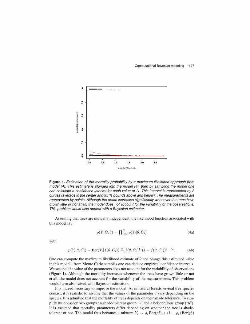
Figure 1. Estimation of the mortality probability by a maximum likelihood approach frommodel (4). This estimate is plunged into the model (4), then by sampling the model onecan calculate a confidence interval for each value of ∆. This interval is represented by 3curves (average in the center and 95 % bounds above and below). The measurements arerepresented by points. Although the death increases significantly whenever the trees havegrown little or not at all, the model does not account for the variability of the observations.This problem would also appear with a Bayesian estimator.

Assuming that trees are mutually independent, the likelihood function associated withthis model is :

p(Y |C, θ) =∏N

i=1 p(Yi|θ, Ci) (4a)

with

p(Yi|θ, Ci) = Ber(Yi|f(θ, Ci))def= f(θ, Ci)Yi(1− f(θ, Ci))1−Yi . (4b)

One can compute the maximum likelihood estimate of θ and plunge this estimated valuein this model : from Monte Carlo samples one can deduce empirical confidence intervals.We see that the value of the parameters does not account for the variability of observations(Figure 1). Although the mortality increases whenever the trees have grown little or notet all, the model does not account for the variability of the measurements. This problemwould have also raised with Bayesian estimators.

It is indeed necessary to improve the model. As in natural forests several tree speciescoexist, it is realistic to assume that the values of the parameter θ vary depending on thespecies. It is admitted that the mortality of trees depends on their shade tolerance. To sim-plify we consider two groups : a shade-tolerant group “s” and a heliophilous group (“h”).It is assumed that mortality parameters differ depending on whether the tree is shade-tolerant or not. The model thus becomes a mixture Yi ∼ ρi Ber(ph

i ) + (1 − ρi) Ber(psi)

A R I M A

Computational Bayesian modeling 129

Y1

µ

1 2 NC C C

NYY2

hyper−paramètres

paramètres

observations

σh,2s s,2σ

θsθh

µh

1 2 Nρ ρρ

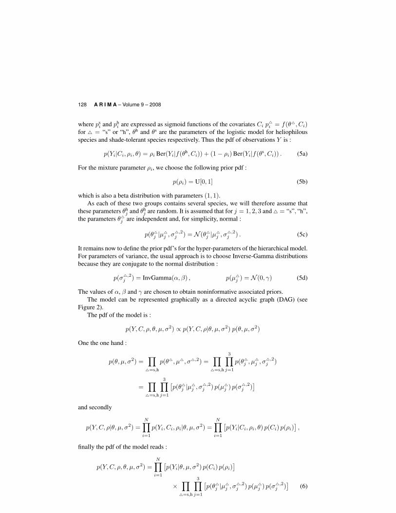
Figure 2. Graphical representation of the model (6) in the form of a directed acyclic graph(DAG). This diagram represents the dependencies of each variable on others. For examplewe can see that Y1 depends on others variables only through C1, ρ1, θh and θs ; we canalso see that conditionally on Y2, C2 is independent of all other variables etc.

where different terms are given by the equations (5) (except that of p(Ci) which is irrele-vant here). Thus the posterior pdf of the parameters is :

p(ρ, θ, µ, σ2|Y, C) ∝N∏

i=1

[p(Yi|θ, µ, σ2) p(ρi)

]×

∏4=s,h

3∏j=1

[p(θ4j |µ

4j , σ4,2

j ) p(µ4j ) p(σ4,2j )

](7)

Although explicit, this expression is not very useful because it is not possible to integrateit in order to calculate estimators like (1). However, the hierarchical nature of the model,represented graphically in Figure 2, will be effectively used by the methods presented inthe next section.

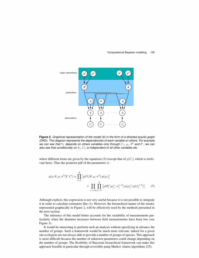
The inference of this model better accounts for the variability of measurements par-ticularly when the diameter increases between field measurements have been low (seeFigure 3).

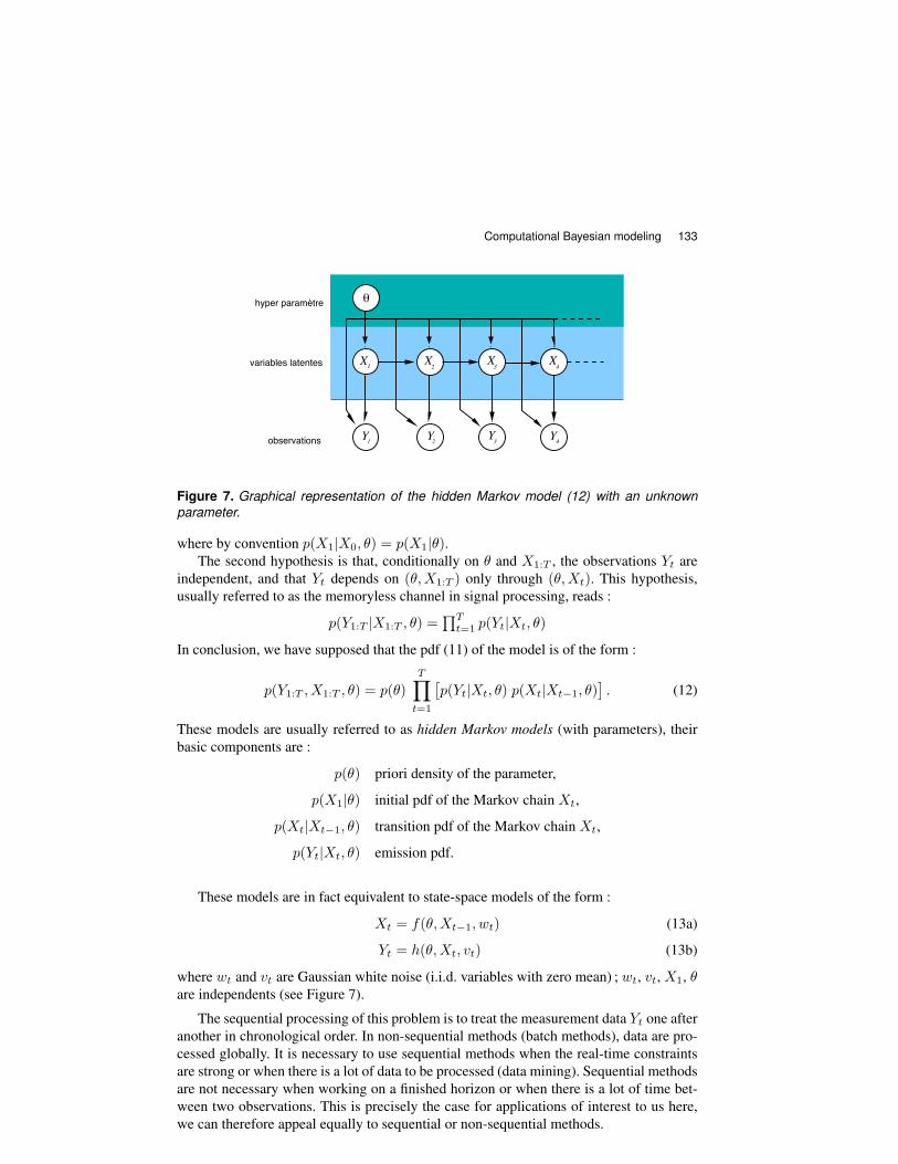
It would be interesting to perform such an analysis without specifying in advance thenumber of groups. Such a framework would be much more relevant, indeed for a givensite ecologists are not always able to provide a number of groups of species. This approachis more difficult because the number of unknown parameters could change depending onthe number of groups. The flexibility of Bayesian hierarchical framework can make thisapproach feasible in particular through reversible jump Markov chains algorithms [25].

A R I M A

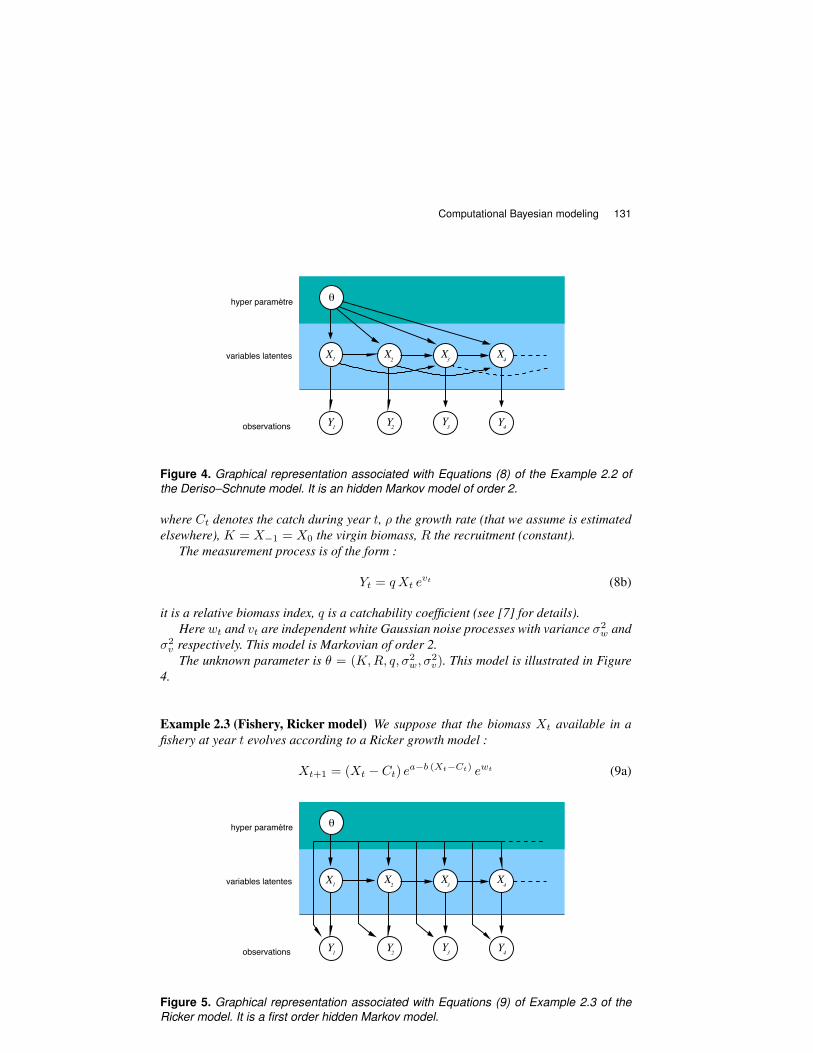
Computational Bayesian modeling 131

3Y

4Y

1X 2X

3X

4X

hyper paramètre

variables latentes

observations

!

1Y 2Y

Figure 4. Graphical representation associated with Equations (8) of the Example 2.2 ofthe Deriso–Schnute model. It is an hidden Markov model of order 2.

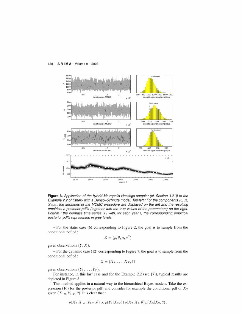
where Ct denotes the catch during year t, ρ the growth rate (that we assume is estimatedelsewhere), K = X−1 = X0 the virgin biomass, R the recruitment (constant).

The measurement process is of the form :

Yt = q Xt evt (8b)

it is a relative biomass index, q is a catchability coefficient (see [7] for details).Here wt and vt are independent white Gaussian noise processes with variance σ2

w andσ2

v respectively. This model is Markovian of order 2.The unknown parameter is θ = (K, R, q, σ2

w, σ2v). This model is illustrated in Figure

4.

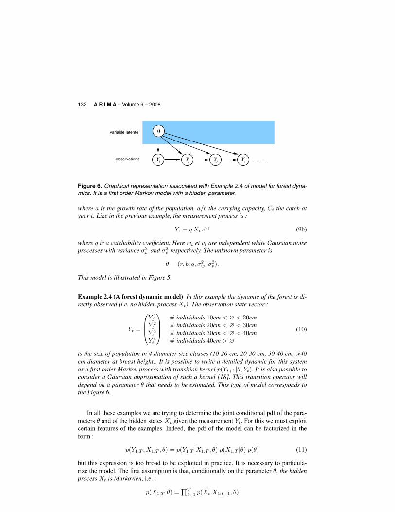
Example 2.3 (Fishery, Ricker model) We suppose that the biomass Xt available in afishery at year t evolves according to a Ricker growth model :

Xt+1 = (Xt − Ct) ea−b (Xt−Ct) ewt (9a)

3Y

4Y

1X 2X

3X

4X

hyper paramètre

variables latentes

observations

!

1Y 2Y

Figure 5. Graphical representation associated with Equations (9) of Example 2.3 of theRicker model. It is a first order hidden Markov model.

A R I M A

Computational Bayesian modeling 133

3Y

4Y

1X 2X

3X

4X

hyper paramètre

variables latentes

observations

!

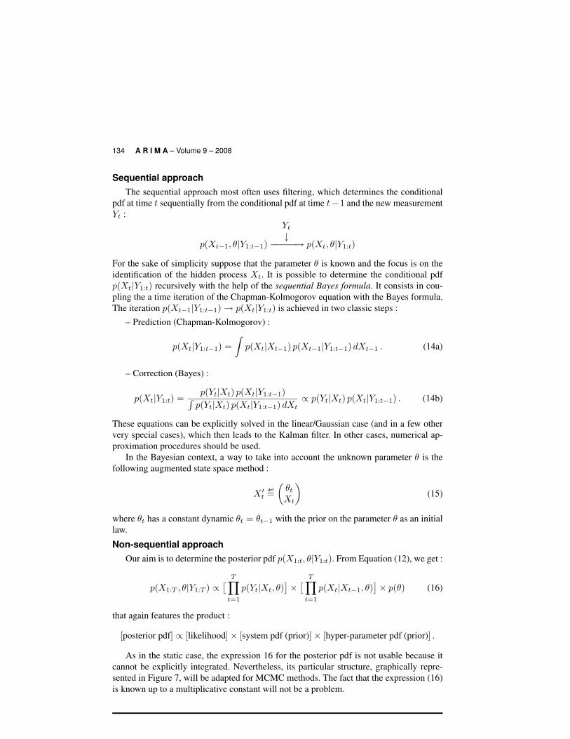
1Y 2Y

Figure 7. Graphical representation of the hidden Markov model (12) with an unknownparameter.

where by convention p(X1|X0, θ) = p(X1|θ).The second hypothesis is that, conditionally on θ and X1:T , the observations Yt are

independent, and that Yt depends on (θ, X1:T ) only through (θ, Xt). This hypothesis,usually referred to as the memoryless channel in signal processing, reads :

p(Y1:T |X1:T , θ) =∏T

t=1 p(Yt|Xt, θ)

In conclusion, we have supposed that the pdf (11) of the model is of the form :

p(Y1:T , X1:T , θ) = p(θ)T∏

t=1

[p(Yt|Xt, θ) p(Xt|Xt−1, θ)

]. (12)

These models are usually referred to as hidden Markov models (with parameters), theirbasic components are :

p(θ) priori density of the parameter,

p(X1|θ) initial pdf of the Markov chain Xt,

p(Xt|Xt−1, θ) transition pdf of the Markov chain Xt,

p(Yt|Xt, θ) emission pdf.

These models are in fact equivalent to state-space models of the form :

Xt = f(θ, Xt−1, wt) (13a)

Yt = h(θ, Xt, vt) (13b)

where wt and vt are Gaussian white noise (i.i.d. variables with zero mean) ; wt, vt, X1, θare independents (see Figure 7).

The sequential processing of this problem is to treat the measurement data Yt one afteranother in chronological order. In non-sequential methods (batch methods), data are pro-cessed globally. It is necessary to use sequential methods when the real-time constraintsare strong or when there is a lot of data to be processed (data mining). Sequential methodsare not necessary when working on a finished horizon or when there is a lot of time bet-ween two observations. This is precisely the case for applications of interest to us here,we can therefore appeal equally to sequential or non-sequential methods.

A R I M A

Computational Bayesian modeling 135

3. Computational Bayesian inference

3.1. IntroductionThe renewal of interest in Bayesian methods mainly originates in the new develop-

ments of Monte Carlo methods [29]. The integration of the posterior pdf (7) in the staticcase, as the integration of the expressions (14) or (16) in the dynamic case cannot bemade explicitly. Monte Carlo methods are specifically adapted for approximation of suchexpressions. This efficiency is also due to the development of pseudo-random number ge-nerators and the ever increasing performance of computers. Monte Carlo methods go farbeyond the question of computational statistics.

The aim of Monte Carlo methods is to approximate deterministic quantities by meansof random simulations. In order to obtain an empirical approximation of a posterior pdfp(θ|Y ), one generate a sample of size N of that pdf :

θ(1), θ(2), . . . , θ(N) iid∼ p(θ|Y ) (17)

then, according to the law of large numbers,

P[θ ∈ B|Y ] ' 1N

N∑i=1

1B(θ(i)) E[φ(θ)|Y ] ' 1N

N∑i=1

φ(θ(i))

that is :

p(θ|Y ) ' pN (θ|Y ) def=1N

N∑i=1

δθ(i) .

Hence pN (θ|Y ) appears to be an empirical approximation of the pdf p(θ|Y ). This isan empirical approximation insofar as it is based on in silico (computer) experimentsof the underlying phenomenon. Monte Carlo methods can therefore be seen as in silicoexperimental methods.

Contemporary Monte Carlo methods are among the algorithms adapted to computers.They were indeed originally developed to be used on the first computer at Los AlamosLaboratory during World War II. Around John von Neumann, scientists like NicholasMetropolis and Stanislaw Ulam are behind the Monte Carlo method in its contemporaryversion (the origins of the method are much older) [34, 26, 32]. These scientists alsoinitiated Monte Carlo Markov chain methods [33].

Here, we do not develop the general aspects of Monte Carlo methods (see [29] for sucha presentation), but will present the Monte Carlo methods that are behind the success ofcomputational Bayesian methods.

3.2. Monte Carlo Markov chains methods (MCMC)It is almost always not possible to sample according to a given target density like

in (17). Let π(z) denote this target density. For some probability distributions – like theuniform distribution, the Gaussian distributions etc. – there are specific algorithms for ge-nerating pseudo-random numbers. Suppose that we did not know easily how to sample ac-cording to the target pdf π(z), but that the analytical expression for this density is known,up to a multiplicative constant (generally this constant is not known and cannot be easilycomputed). The aim of the method is to (numerically) build a Markov chain (Z(k))k≥0

whose limit density is precisely π(z). By simulating sufficiently many iterations of this

A R I M A

Computational Bayesian modeling 137

and suppose that we know how to sample from the conditional marginal pdf’s :

qpropt (z′t|z¬t) = p(Zt = z′t|Z¬t = z¬t) (19)

where Z¬t = {Z¬s ; s = 1 · · ·T ; s 6= t}.Starting from an initial configuration Z

(0)1:T , the method propose to select t at random

(or sequentially) and to update the component t by letting :

Z(k+1)t ∼ qprop

t ( · |Z(k)¬t )

where other components remain unchanged, i.e. Z(k+1)s = Z

(k)s for s 6= t. This method

is presented in Algorithm 2.

choose an initial configuration z1:T

for k = 1, 2 . . . dochoose t at random in {1, . . . , T}zt ∼ p(Zt|Z¬t = z¬t)

end forAlgorithm 2: Gibbs sampler.

3.2.3. Hybrid Metropolis-Hastings samplerSuppose now that we do not know how to sample according to the conditional margi-

nal pdf’s (19). One can use at each iteration of the Gibbs sampler, a Metropolis-Hastingstechnique : instead of qprop

t (z′t|z¬t) defined by (19), we consider a proposition kernel anduse an acceptance/rejection technique like in (18b). This leads to the hybrid Metropolis-Hastings method (also called “Metropolis within Gibbs” sampler). It is necessary to de-compose the marginal conditional pdf’s as follows :

p(Zt|Z¬t) ∝ qpropt (Zt|Z¬t)︸ ︷︷ ︸

proposition kernel

× λt(Zt, Z¬t)︸ ︷︷ ︸likelihood

(20)

This method leads to Algorithm 3.

choose an initial configuration z1:T

for k = 1, 2 . . . dofor t = 1 : T do

z′t ∼ qpropt ( · |z¬t) {generate a candidate}

α← λt(z′t, z¬t)/λt(zt, z¬t) {cf. Equation (20)}if α > rand() then

zt ← z′t {the new configuration is accepted}end if

end forend for

Algorithm 3: Hybrid Metropolis-Hastings sampler (rand() is the uniform law ge-nerator U [0, 1]).

3.2.4. ApplicationThe Hybrid Metropolis-Hastings sampler can potentially be applied to all hierarchical

Bayes models presented in Section 2 :

A R I M A

Computational Bayesian modeling 139

hence, the decomposition (20) could be :

qprop(X2|X¬2)def= p(X2|X1, θ) ,

λ(X2|X¬2)def= p(Y2|X2, θ) p(X3|X2, θ)

(The other components of X1:T and θ are treated the same way). This choice for theproposal kernel qprop(X2|X¬2) is perhaps not the most efficient, but it applies to all hierar-chical Bayes models and all hidden Markov models.

MCMC methods are extremely successful. Indeed, they are simple to set, they allowmany variants and can be applied to many problems. They can be interconnected withother Monte Carlo methods and can be applied to hidden Markov models and to hierar-chical Bayes models. This success is also due to software like WinBUGS or OpenBUGS(that also can be called from inside the R statistical package).

However, these methods may feature poor mixing properties and can be very slow.This is particularly the case with nonlinear systems in high dimension like the systemsanalyzed here by the hybrid Metropolis-Hastings method.

This latter approach is used extensively because in many situations it is the only me-thod that can be applied. Current effort is focused on interacting parallel versions of suchmethods [5] and on the comparisons with other methods [19].

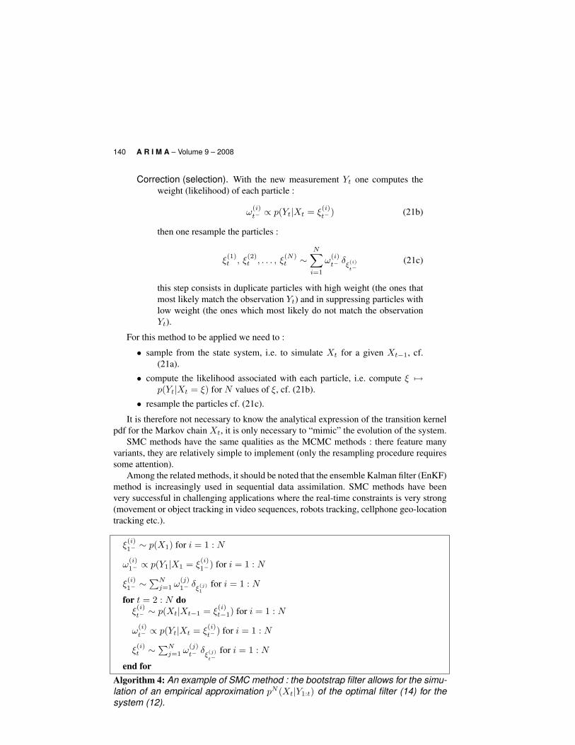
3.3. Sequential Monte Carlo methods (SMC)Equations (14) for the nonlinear optimal filter can be used in practice. The purpose

of the Monte Carlo sequential methods, also called particle filters, is to propose a MonteCarlo approximation of the optimal filter. These methods are now widely developed inpractice and have a mathematical framework [, 14]. They were proposed in their presentform in the early 1990’s [24].

For the sake of simplicity, we consider Equations (14), i.e. without unknown parame-ter. The goal of the SMC method is to propose an empirical approximation of p(Xt|Y1:t) :

p(Xt|Y1:t) ' pN (Xt|Y1:t) =1N

N∑i=1

δξ(i)t

(Xt) .

here the question is to determine the positions ξ(i)t of the N particles. It is also possible to

seek an importance sampling approximation :

p(Xt|Y1:t) ' pN (Xt|Y1:t) =N∑

i=1

ω(i)t δ

ξ(i)t

(Xt) .

and the question here is to determine the positions ξ(i)t and weights ω

(i)t of the N particles.

For the bootstrap approximation, which is the simplest implementation of SMC me-thods, the iteration pN (Xt−1|Y1:t−1)→ pN (Xt|Y1:t) is in two steps :

Prediction (mutation). For each i = 1, . . . , N , one compute the predictedparticle positions with the help of the transition kernel p(Xt|Xt−1) ofthe Markov chain :

ξ(i)t− ∼ p(Xt|Xt−1 = ξ

(i)t−1) (21a)

independently of one another.

A R I M A

Computational Bayesian modeling 141

3.4. ComparisonMCMC and SMC differs on 3 essential points :

• MCMC methods are iterative methods and SMC are not. SMC methodssequentially process the observations Yt for t = 1 to T . MCMC methods areiterative and questions of diagnosing convergence is quite difficult.• SMC methods (in their basic versions) approximate p(Xt|Y1:t) while

MCMC methods approximate p(Xt|Y1:T ). The first is a filtering problem,the second is a smoothing problem. Smoothing methods for SMC are not yetwell developed. The difference is important : for t = 1 in the SMC case oneconsiders p(X1|Y1) whereas in the MCMC case one considers p(X1|Y1:T ).The variance of the latter expression is lower.• Taking into account the identification of unknown parameters is very

different in the two approaches. MCMC methods take these into account ina natural way. For SMC methods, the state augmentation method (15) has itslimits. Alternative SMC methods using kernel techniques could be applied[6].

An important point is that all SMC methods have been developed with expressed aimof being applied to real-time applications. This constraint does not exist in the applicationsconsidered here. It is therefore possible to use cumbersome methods. One natural idea isto use MCMC methods to propagate particles (see for example the “resample-move” al-gorithm proposed by Gilks and Berzuini [21]). Instead of propagating particles accordingto the transition kernel of the Markov chain (cf. (21a)), one can proposed sampling froma more relevant target pdf with a MCMC technique.

4. ConclusionsDuring the past fifteen years, Monte Carlo methods have developed considerably.

They provide a computational framework for Bayesian inference methods. Comparedwith frequentist approaches, Bayesian approaches are best suited to applications in eco-logy where one usually has limited amount of data. There is now percolation betweenapplication, probability modeling and computational inference. One reason for this suc-cess is the availability of efficient software accessible from widespread platforms like R.Statistical inference was often wrongly opposed to modeling, notably to deterministic mo-deling. With the development of Markov modeling, inference and modeling have formeda fruitful dual relationship. The couple Markov modeling and Bayesian inference now fitsin a computational framework which makes it a powerful tool for in silico experiment andanalysis.

5. Bibliographie

[1] J. O. Berger. Statistical Decision Theory and Bayesian Analysis. Springer–Verlag, 1985. 2ndEdition.

[2] S. P. Brooks. Bayesian computation : A statistical revolution. Transactions of the Royal Society,Series A, 361 :2681–2697, 2003.

[3] S. P. Brooks and G. O. Roberts. Convergence assessment techniques for Markov chain MonteCarlo. Statistics and Computing, 8(4) :319–335, 1998.

A R I M A

Computational Bayesian modeling 143

[25] P. J. Green. Reversible jump MCMC computation and Bayesian model determination. Bio-metrika, 82(4) :711–732, December 1995.

[26] F. Harlow and N. Metropolis. Computing and computers – weapons simulation leads to thecomputer era. Los Alamos Science, 7 :132–141, 1983.

[27] D. Howie. Interpreting probability : Controversies and developments in the early twentiethcentury. Cambridge University Press, 2002.

[28] R. E. Kass, B. P. Carlin, A. Gelman, and R. M. Neal. Markov Chain Monte Carlo in practice :A roundtable discussion. The American Statistician, 52 :93–100, 1998.

[29] J. S. Liu. Monte Carlo Strategies in Scientific Computing. Springer–Verlag, New York, 2001.

[30] D. Malakoff. Bayes offers a “new” way to make sense of numbers. Science, 286 :1460–1464,1999.

[31] J.-M. Marin and C. P. Robert. Bayesian Core : A Practical Approach to Computational Baye-sian Statistics. Springer-Verlag, 2007.

[32] N. Metropolis. The beginning of the Monte Carlo method. Los Alamos Science, 15 :125–130,1987.

[33] N. Metropolis, A. W. Rosenbluth, M. N. Rosenbluth, A. H. Teller, and E. Teller. Equation ofstate calculations by fast computing machines. The Journal of Chemical Physics, 21(6) :1087–1091, 1953.

[34] N. Metropolis and S. Ulam. The Monte Carlo method. Journal of the American StatisticalAssociation, 44(247) :335–341, February 1949.

[35] R. Meyer and R. B. Millar. Bayesian stock assessment using a state-space implementation ofthe delay difference model. Canadian Journal of Fisheries and Aquatic Sciences, 56 :37–52,1999.

[36] A. E. Punt and R. Hilborn. Fisheries stock assessment and decision analysis : the Bayesianapproach. Reviews in Fish Biology and Fisheries, 7 :35–63, 1997.

[37] K. H. Reckhow. Bayesian approaches in ecological analysis and modeling. In C. D. Canham,J. J. Cole, and W. K. Lauenroth, editors, Models in ecosystem science, pages 168–183. PrincetonUniversity Press, Princeton, New Jersey, USA., 2003.

[38] E. Rivot, E. Prevost, E. Parent, and J.-L. Blaginière. A Bayesian state-space modelling frame-work for fitting a salmon stage-structured population dynamic model to multiple time series offield data. Ecological Modelling, 179 :463–485, 2004.

[39] Carl J. Schwarz and George A. F. Seber. Estimating animal abundance : Review III. StatisticalScience, 14(4) :427–456, 1999.

[40] L. Tierney. Markov chains for exploring posterior distributions (with discussion). The Annalsof Statistics, 22(4) :1701–1728, December 1994.

[41] J. R. Webster. Hierarchy theory and ecosystem models. In E. Halfon, editor, Theoreticalsystems ecology, pages 119–129. Academic Press, 1978.

A R I M A