Bayesian Inference - Wellcome Trust Centre for …€¢ Some probability densities/distributions •...
50
Bayesian Inference Thomas Nichols With thanks Lee Harrison
Transcript of Bayesian Inference - Wellcome Trust Centre for …€¢ Some probability densities/distributions •...

Bayesian Inference
Thomas Nichols
With thanks Lee Harrison
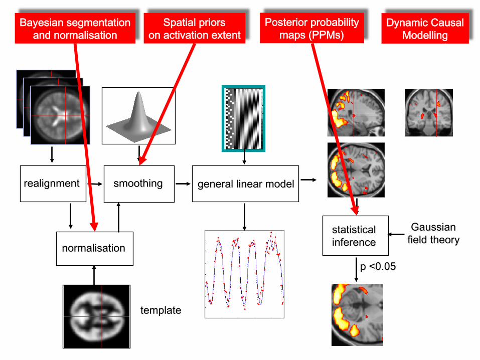
Bayesian segmentation and normalisation
Spatial priors on activation extent
Dynamic Causal Modelling
Posterior probability maps (PPMs)

Paradigm Results
Attention to Motion
Büchel & Friston 1997, Cereb. Cortex Büchel et al. 1998, Brain
V5+
SPC V3A
Attention – No attention
- fixation only - observe static dots + photic V1 - observe moving dots + motion V5 - task on moving dots + attention V5 + parietal cortex
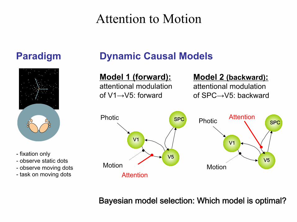
Paradigm
- fixation only - observe static dots - observe moving dots - task on moving dots
Dynamic Causal Models
Attention to Motion
V1
V5
SPC
Motion
Photic
Attention
V1
V5
SPC
Motion
Photic Attention
Model 1 (forward): attentional modulation of V1→V5: forward
Model 2 (backward): attentional modulation of SPC→V5: backward
Bayesian model selection: Which model is optimal?

Responses to Uncertainty Long term memory
Short term memory
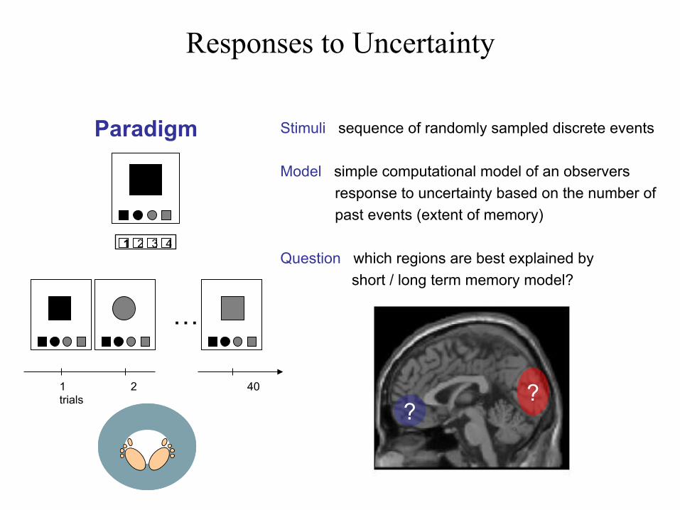
Responses to Uncertainty
Paradigm Stimuli sequence of randomly sampled discrete events
Model simple computational model of an observers response to uncertainty based on the number of past events (extent of memory)
Question which regions are best explained by short / long term memory model?
…
1 2 40 trials
1 4 3 2
? ?

Overview
• Introductory remarks
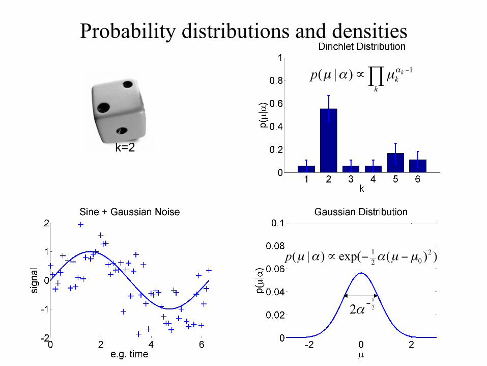
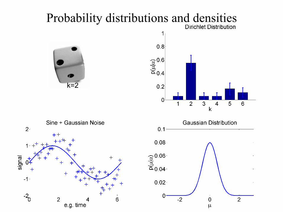
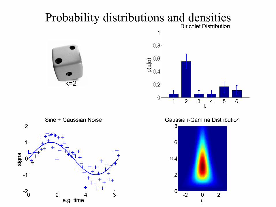
• Some probability densities/distributions
• Probabilistic (generative) models
• Bayesian inference
• A simple example – Bayesian linear regression
• SPM applications – Segmentation – Dynamic causal modeling – Spatial models of fMRI time series

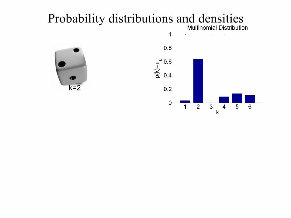
k=2
Probability distributions and densities

Probability distributions and densities
k=2
Probability distributions and densities
k=2
Probability distributions and densities
k=2
Probability distributions and densities
k=2

Probability distributions and densities
k=2
Probability distributions and densities
k=2

Generative models estimation
time
space
generation
space
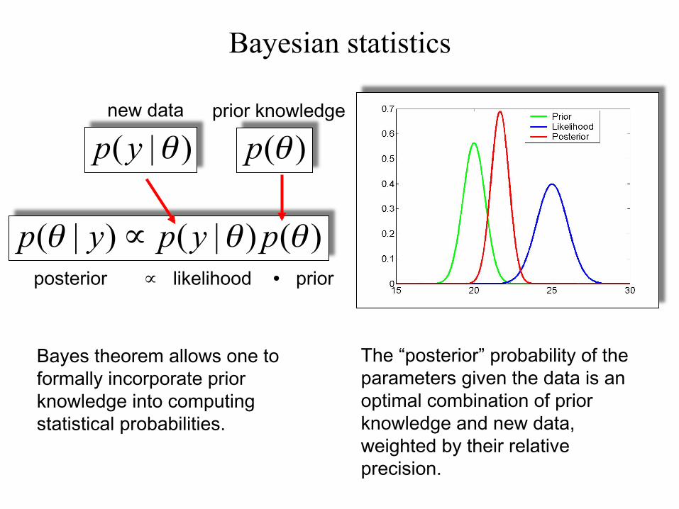
posterior ∝ likelihood ∙ prior
Bayes theorem allows one to formally incorporate prior knowledge into computing statistical probabilities.
The “posterior” probability of the parameters given the data is an optimal combination of prior knowledge and new data, weighted by their relative precision.
new data prior knowledge
Bayesian statistics

Given data y and parameters θ, their joint probability can be written in 2 ways:
Eliminating p(y,θ) gives Bayes’ rule:
Likelihood Prior
Evidence
Posterior
Bayes’ rule

y Observation of data
likelihood p(y|θ)
prior distribution p(θ)
Formulation of a generative model
Update of beliefs based upon observations, given a prior state of knowledge
Principles of Bayesian inference

Normal densities Univariate Gaussian
Posterior mean = precision-weighted combination of prior mean and data mean
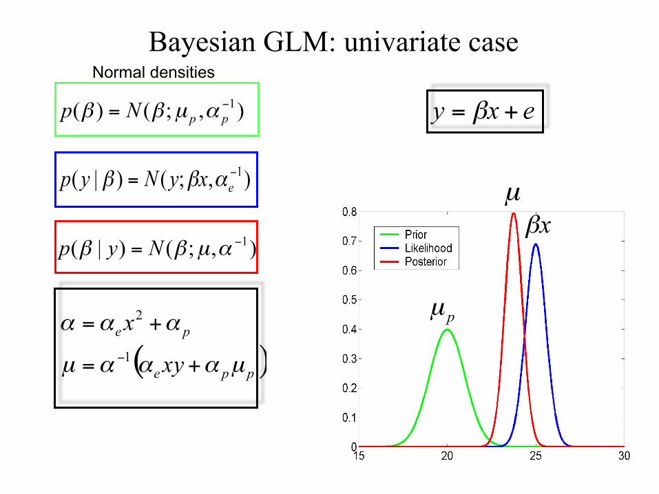
Normal densities Bayesian GLM: univariate case
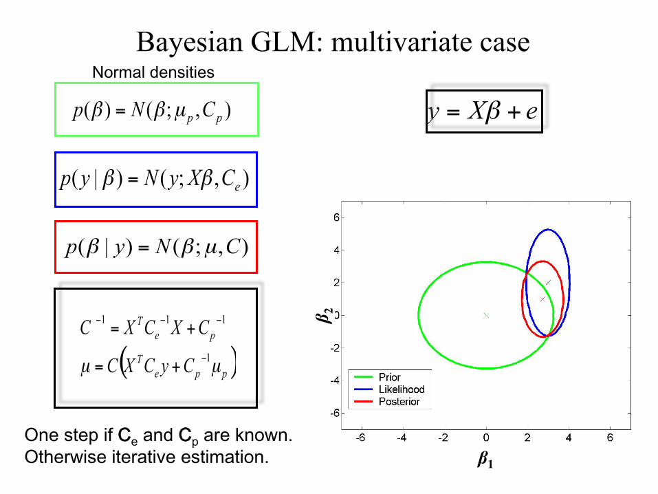
Normal densities Bayesian GLM: multivariate case
β 2
β1
One step if Ce and Cp are known. Otherwise iterative estimation.

Approximate inference: optimization
True posterior
Approximate posterior
iteratively improve
free energy
mean-field approximation
Value of parameter
Objective function

Simple example – linear regression Data Ordinary least squares

Simple example – linear regression
Bases (explanatory variables)
Data and model fit
Bases (explanatory variables) Sum of squared errors
Ordinary least squares

Simple example – linear regression Data and model fit
Bases (explanatory variables)
Ordinary least squares
Sum of squared errors

Simple example – linear regression Data and model fit
Bases (explanatory variables) Sum of squared errors
Ordinary least squares
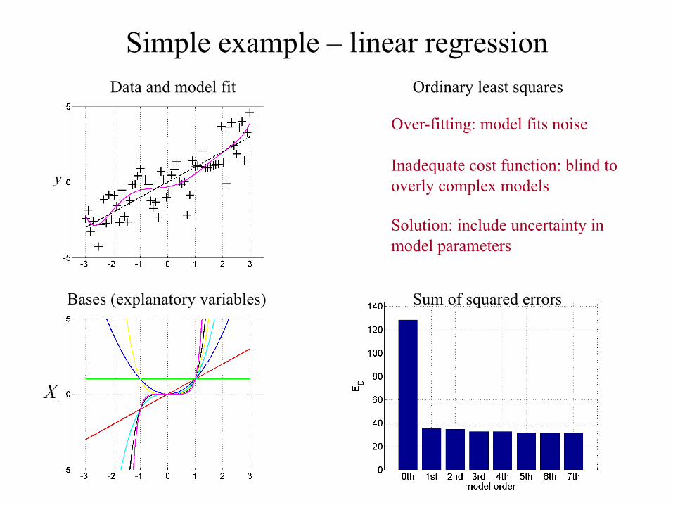
Simple example – linear regression Data and model fit
Bases (explanatory variables) Sum of squared errors
Over-fitting: model fits noise
Inadequate cost function: blind to overly complex models
Solution: include uncertainty in model parameters
Ordinary least squares
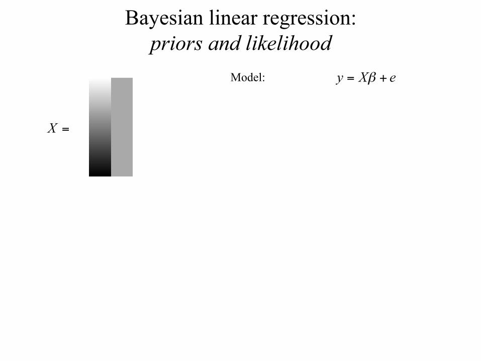
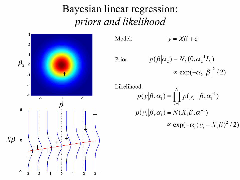
Bayesian linear regression: priors and likelihood
Model:

Bayesian linear regression: priors and likelihood
Model:
Prior:

Sample curves from prior (before observing any data)
Mean curve
Bayesian linear regression: priors and likelihood
Model:
Prior:

Bayesian linear regression: priors and likelihood
Model:
Prior:
Likelihood:

Bayesian linear regression: priors and likelihood
Model:
Prior:
Likelihood:
Bayesian linear regression: priors and likelihood
Model:
Prior:
Likelihood:

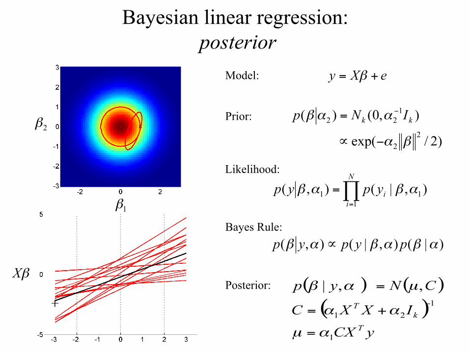
Bayesian linear regression: posterior
Model:
Prior:
Likelihood:
Bayes Rule:
Bayesian linear regression: posterior
Model:
Prior:
Likelihood:
Bayes Rule:
Posterior:

Bayesian linear regression: posterior
Model:
Prior:
Likelihood:
Bayes Rule:
Posterior:

Bayesian linear regression: posterior
Model:
Prior:
Likelihood:
Bayes Rule:
Posterior:
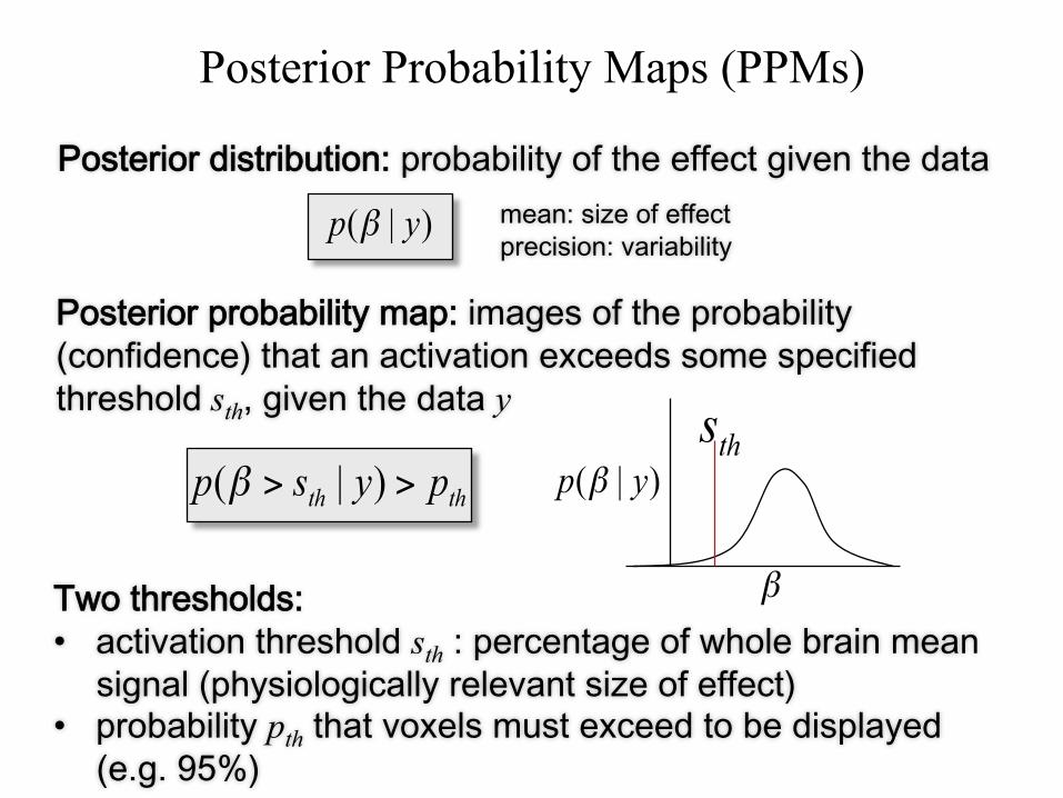
Posterior distribution: probability of the effect given the data
Posterior probability map: images of the probability (confidence) that an activation exceeds some specified threshold sth, given the data y
Two thresholds: • activation threshold sth : percentage of whole brain mean
signal (physiologically relevant size of effect) • probability pth that voxels must exceed to be displayed
(e.g. 95%)
mean: size of effectprecision: variability
Posterior Probability Maps (PPMs)

Bayesian linear regression: model selection
Bayes Rule:
normalizing constant
Model evidence:
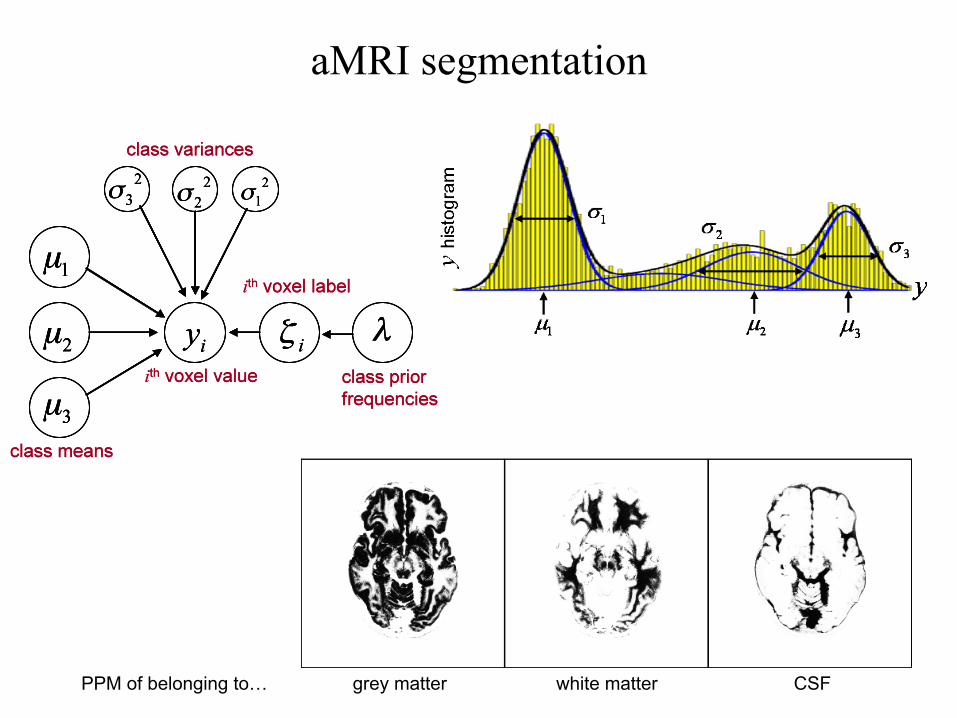
grey matter PPM of belonging to… CSF white matter
aMRI segmentation
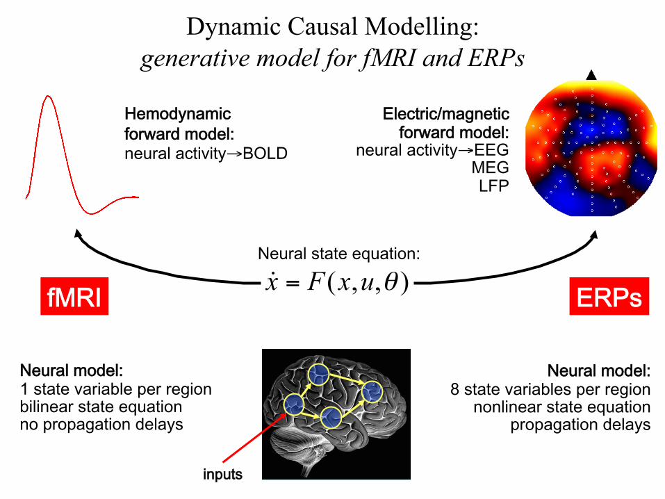
Neural state equation:
Electric/magnetic forward model:
neural activity→EEGMEG LFP
Neural model: 1 state variable per region bilinear state equation no propagation delays
Neural model: 8 state variables per region
nonlinear state equation propagation delays
fMRI ERPs
inputs
Hemodynamicforward model:neural activity→BOLD
Dynamic Causal Modelling: generative model for fMRI and ERPs

m2 m1 m3 m4
V1 V5 stim
PPC
attention
V1 V5 stim
PPC
attention
V1 V5 stim
PPC
attention
V1 V5 stim
PPC
attention
[Stephan et al., Neuroimage, 2008]
m1 m2 m3 m4
15
10
5
0
V1 V5 stim
PPC
attention
1.25
0.13
0.46
0.39 0.26
0.26
0.10 estimated
effective synaptic strengths for best model (m4)
models marginal likelihood
Bayesian Model Selection for fMRI

AR coeff (correlated noise)
prior precision of AR coeff
VB estimate of β ML estimate of β
aMRI Smooth Y (RFT)
fMRI time series analysis with spatial priors
observations
GLM coeff
prior precision of GLM coeff
prior precision of data noise
Penny et al 2005
degree of smoothness Spatial precision matrix
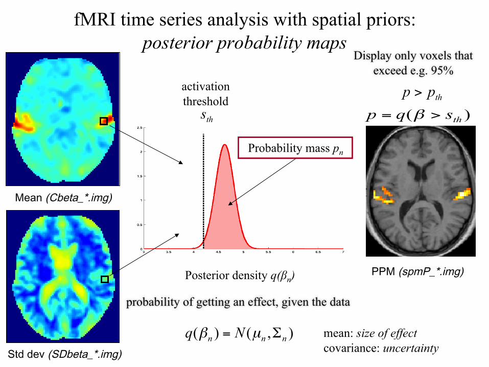
Mean (Cbeta_*.img)
Std dev (SDbeta_*.img)
activation threshold
Posterior density q(βn)
Probability mass pn
fMRI time series analysis with spatial priors: posterior probability maps
probability of getting an effect, given the data
mean: size of effect covariance: uncertainty
Display only voxels that exceed e.g. 95%
PPM (spmP_*.img)

fMRI time series analysis with spatial priors: Bayesian model selection
Compute log-evidence for each model/subject
model 1
model K
subject 1
subject N
Log-evidence maps
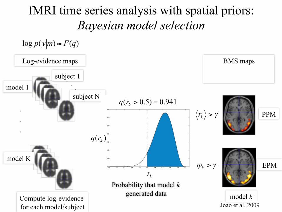
fMRI time series analysis with spatial priors: Bayesian model selection
BMS maps
PPM
EPM
model k Joao et al, 2009
Compute log-evidence for each model/subject
model 1
model K
subject 1
subject N
Log-evidence maps
Probability that model k generated data

Reminder… Long term memory
Short term memory

Short-term memory model long-term memory model
onsets Missed trials
IT indices: H,h,I,i
H=entropy; h=surprise; I=mutual information; i=mutual surprise
Compare two models
IT indices are smoother

primary visual cortex
Regions best
explained by short-
term memory model
Regions best explained by
long-term memory model
frontal cortex (executive
control)
Group data: Bayesian Model Selection maps

Thank-you