Computational Elements For Strapdown Systems

Paul G. SavageStrapdown Associates, Inc.

Maple Plain, Minnesota 55359 USA

WBN-14010www.strapdownassociates.com

May 31, 2015

Originally published inNATO Research and Technology Organization (RTO)

Sensors and Electronics Technology Panel (SET)Low-Cost Navigation Sensors and Integration Technology

RTO EDUCATIONAL NOTES RTO-SET-116(2008), Section 9Published in 2009

ABSTRACT

This paper provides an overview of the primary strapdown inertial system computationalelements and their interrelationship. Using an aircraft type strapdown inertial navigation systemas a representative example, the paper provides differential equations for attitude, velocity,position determination, associated integral solution functions, and representative algorithms forsystem computer implementation. For the inertial sensor errors, angular rate sensor andaccelerometer analytical models are presented including associated compensation algorithms forcorrection in the system computer. Sensor compensation techniques are discussed for coning,sculling, scrolling computation algorithms and for accelerometer output adjustment for physicalsize effect separation and anisoinertia error. Navigation error parameters are described andrelated to errors in the system computed attitude, velocity, position solutions. Differentialequations for the navigation error parameters are presented showing error parameter propagationin response to residual inertial sensor errors (following sensor compensation) and to errors in thegravity model used in the system computer.

COORDINATE FRAMES

As used in this paper, a coordinate frame is an analytical abstraction defined by three mutuallyperpendicular unit vectors. A coordinate frame can be visualized as a set of three perpendicularlines (axes) passing through a common point (origin) with the unit vectors emanating from theorigin along the axes. In this paper, the physical position of each coordinate frame’s origin isarbitrary. The principal coordinate frames utilized are the following:

B Frame = "Body" coordinate frame parallel to strapdown inertial sensor axes.

1

N Frame = "Navigation" coordinate frame having Z axis parallel to the upward verticalat the local position location. A "wander azimuth" N Frame has thehorizontal X, Y axes rotating relative to non-rotating inertial space at thelocal vertical component of earth's rate about the Z axis. A "free azimuth" NFrame would have zero inertial rotation rate of the X, Y axes around the Zaxis. A "geographic" N Frame would have the X, Y axes rotated around Z tomaintain the Y axis parallel to local true north.

E Frame = "Earth" referenced coordinate frame with fixed angular geometry relative tothe rotating earth.

I Frame = "Inertial" non-rotating coordinate frame.

NOTATION

V = Vector without specific coordinate frame designation. A vector is a parameter thathas length and direction. Vectors used in the paper are classified as “free vectors”,hence, have no preferred location in coordinate frames in which they areanalytically described.

VA = Column matrix with elements equal to the projection of V on Coordinate Frame Aaxes. The projection of V on each Frame A axis equals the dot product of V withthe coordinate Frame A axis unit vector.

VA × = Skew symmetric (or cross-product) form of VA represented by the square

matrix

0 - VZA VYA

VZA 0 - VXA

- VYA VXA 0

in which VXA , VYA , VZA are the

components of VA. The matrix product of VA × with another A Frame

vector equals the cross-product of VA with the vector in the A Frame.

CA2

A1 = Direction cosine matrix that transforms a vector from its Coordinate Frame A2

projection form to its Coordinate Frame A1 projection form.

ωA1A2 = Angular rate of Coordinate Frame A2 relative to Coordinate Frame A1. When

A1 is non-rotating, ωA1A2 is the angular rate that would be measured by

angular rate sensors mounted on Frame A2.

.

= d dt

= Derivative with respect to time.

t = Time.

2

1. INTRODUCTION

The primary computational elements in a strapdown inertial navigation system (INS) consistof integration operations for calculating attitude, velocity and position navigation parametersusing strapdown angular rate and specific force acceleration for input. The computational formof these operations originate from two basic sources: time rate differential equations for thenavigation parameters and analytical error models describing the error characteristics of thestrapdown inertial angular rate sensors and accelerometers providing the angular rate and specificforce acceleration measurement data. The latter is the source for compensation algorithms usedin the system computer to correct predictable errors in the inertial sensor outputs. The former isthe source for digital integration algorithms resident in system software for computing thenavigation parameters. Both are the source for error propagation equations used to describe thebehavior of navigation parameter errors in the presence of residual sensor errors remaining aftercompensation.

This paper provides examples of each of the aforementioned computational elements and theirinterrelationship. For the digital integration algorithms, the examples are selected to emphasizea structural goal of being based (to the greatest extent possible) on closed-form analytically exactintegral solutions to the navigation parameter time rate differential equations. Such a structuresignificantly simplifies the integration algorithm software validation process based on acomparison with closed-form exact solution dynamic model simulators designed to thoroughlyexercise the exact solution algorithms under test (Reference 26). For properly derived andprogrammed algorithms, the comparison will yield identically zero difference, thereby providinga clear unambiguous algorithm software validation. Once validated, such algorithms can be usedas a generic set suitable for all strapdown inertial applications. Associated algorithmdocumentation is also simplified because algorithm derivations are classical analyticalformulations and explanations/numerical-error-analysis justification for application dependentapproximations are not required because there are none. Modern day strapdown systemcomputer technology (high throughput, long floating point word-length) allows the general useof such exact solution algorithms without penalty. Similarly, the sensor compensationalgorithms shown in the paper are a generic set based on the exact inverse of classical sensorerror models without first order approximations (as has been commonly used in the past to saveon computer throughput).

The form of the navigation error propagation equations are based on analytical definitions ofthe attitude, velocity, position error parameters. Several choices are possible. Two of the mostcommon sets are illustrated in the paper and equivalencies between the two described. Anexample of the error propagation equations based on one of the sets is provided.

This paper is an updated version of Reference 22. Reference 22 is a condensed summary ofmaterial originally published in the two volume textbook Strapdown Analytics (Ref. 20), thesecond edition of which has been recently published (Reference 25). Strapdown Analyticsprovides a broad detailed exposition of the analytical aspects of strapdown inertial navigationtechnology. This version of the Reference 22 paper also incorporates new material from therecently published paper A Unified Mathematical Framework For Strapdown Algorithm Design(Reference 23) - also provided in Section 19.1 of the second edition of Strapdown Analytics

3

(Reference 25). Equations in this paper (as in Reference 22) are presented without proof. Theirderivations are provided in Reference 20 (or 25) and in Reference 23 as delineated throughoutthe paper (by Reference 20 or 25 section number and by Reference 23 equation number).Documents delineated in the paper's References listing that are not cited in the body of the paperare those cited in Reference 20 (or 25) that are specifically related to the paper's subject matter.

2. REPRESENTATIVE STRAPDOWN INERTIAL NAVIGATIONDIFFERENTIAL EQUATIONS

This section describes a typical set of basic attitude/velocity/position integration andacceleration transformation operations performed in a strapdown INS. The integrationoperations are described in the form of continuous differential equations that when integrated inthe classical analytical continuous sense, provide the attitude, velocity and position datagenerated digitally in the strapdown system computer. The algorithms described in Section 4 aredesigned to achieve the same numerical result by digital integration as the continuous integrationof the differential equations presented in this section.

2.1 Attitude

For a terrestrial (earth) based inertial navigation system (e.g., for aircraft), sensor assemblyangular attitude orientation is usually described as an “attitude direction cosine matrix” (orattitude quaternion) relating sensor assembly axes (the “body” or B Frame) to locally levelattitude reference coordinates (N Frame). Attitude determination consists of integrating theassociated time rate differential equations for the selected attitude parameters. For an attitudereference formulation based on direction cosines the attitude time rate differential equations aregiven by (Ref. 20 (or 25) Sects. 4.1 and 4.1.1):

CB

.N = CB

N ωIB

B × - ωIN

N × CB

N

ωIEN

= CNE T

ωIE E

ωENN

≡ ρN = FC

N uUp

N × vN + ρZN uZN

N (1)

ωINN

= ωIEN

+ ωENN

where

ρN = Conventional notation for ωEN

N, also known as “transport rate”, and analytically

defined as the angular rate of Frame N relative to Frame E.

ρZN = Vertical component of ρN. For a "wander azimuth" N Frame, ρZN is zero. For a

"free azimuth" N Frame, ρZN is the downward vertical component of earth's

inertial angular rate.

4

FCN

= Curvature matrix in the N Frame that is a function of position location over the

earth.

v = Velocity (rate of change of position) relative to the earth.

uUp = Unit vector upward at the current position location (parallel to the N Frame Z

axis).

The equivalent quaternion formulation (Ref. 20 (or 25) Sect. 4.1) is as follows:

qB

.N = 12

qBN

ωIBB

- 12

ωINN

qBN

(2)

where

qBN

= Attitude quaternion relating coordinate Frames B and N.

ωIBB

, ωINN

= Quaternions with vector components equal to ωIBB

, ωINN

and zero for the

scalar components.

The CNE

matrix in Equations (1) defines the system angular position location in earth reference

coordinates, hence, is sometimes denoted as the “position” direction cosine matrix (or the

equivalent position quaternion). The CNE

matrix is calculated by integrating its differential

equation (described in Section 2.3) using ωINN

(N Frame "platform" rotation rate) as input. For

earth's zero altitude surface reference modeled as an ellipsoid of revolution around earth'srotation axis (i.e., the conventional approach), Reference 20 (or 25) Sections 5.2.4 and 5.3

develop the following exact expression for the FCN

curvature matrix in Equations (1) based on an

E Frame definition having Y axis parallel to earth's axis of rotation:

FCN

=

FC11 FC12 0

FC21 FC22 0

0 0 0

FC11 = 1rl

1 + D212

feh FC12 = 1rl

D21 D22 feh (3)

FC21 = 1rl

D21 D22 feh FC22 = 1rl

1 + D222

feh

(Continued)

5

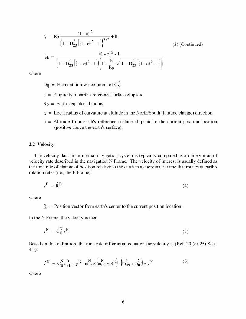
rl = R0 (1 - e) 2

1 + D232

1 - e 2 - 1 3 / 2

+ h

(3) (Continued)

feh ≡ 1 - e 2 - 1

1 + D232

1 - e 2 - 1 1 + h

R0 1 + D23

2 1 - e 2 - 1

where

Dij = Element in row i column j of CNE

.

e = Ellipticity of earth's reference surface ellipsoid.

R0 = Earth's equatorial radius.

rl = Local radius of curvature at altitude in the North/South (latitude change) direction.

h = Altitude from earth's reference surface ellipsoid to the current position location(positive above the earth's surface).

2.2 Velocity

The velocity data in an inertial navigation system is typically computed as an integration ofvelocity rate described in the navigation N Frame. The velocity of interest is usually defined asthe time rate of change of position relative to the earth in a coordinate frame that rotates at earth'srotation rates (i.e., the E Frame):

vE ≡ R.

E (4)

where

R = Position vector from earth's center to the current position location.

In the N Frame, the velocity is then:

vN = CEN

vE (5)

Based on this definition, the time rate differential equation for velocity is (Ref. 20 (or 25) Sect.4.3):

v.N = CB

N aSF

B + gN - ωIE

N × ωIE

N × RN - ωIN

N + ωIE

N × vN (6)

where

6

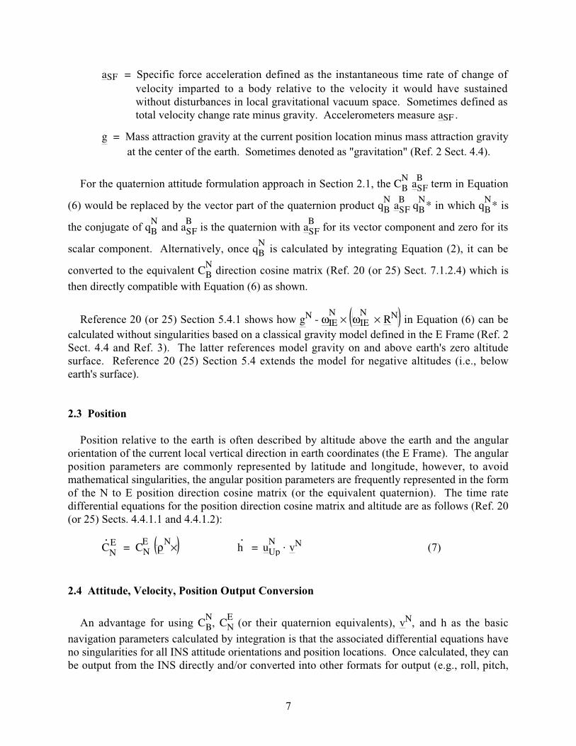
aSF = Specific force acceleration defined as the instantaneous time rate of change of

velocity imparted to a body relative to the velocity it would have sustainedwithout disturbances in local gravitational vacuum space. Sometimes defined astotal velocity change rate minus gravity. Accelerometers measure aSF .

g = Mass attraction gravity at the current position location minus mass attraction gravity

at the center of the earth. Sometimes denoted as "gravitation" (Ref. 2 Sect. 4.4).

For the quaternion attitude formulation approach in Section 2.1, the CBN

aSFB

term in Equation

(6) would be replaced by the vector part of the quaternion product qBN

aSFB

qBN

* in which qBN

* is

the conjugate of qBN

and aSFB

is the quaternion with aSFB

for its vector component and zero for its

scalar component. Alternatively, once qBN

is calculated by integrating Equation (2), it can be

converted to the equivalent CBN

direction cosine matrix (Ref. 20 (or 25) Sect. 7.1.2.4) which is

then directly compatible with Equation (6) as shown.

Reference 20 (or 25) Section 5.4.1 shows how gN - ωIEN

× ωIE N

× RN in Equation (6) can be

calculated without singularities based on a classical gravity model defined in the E Frame (Ref. 2Sect. 4.4 and Ref. 3). The latter references model gravity on and above earth's zero altitudesurface. Reference 20 (25) Section 5.4 extends the model for negative altitudes (i.e., belowearth's surface).

2.3 Position

Position relative to the earth is often described by altitude above the earth and the angularorientation of the current local vertical direction in earth coordinates (the E Frame). The angularposition parameters are commonly represented by latitude and longitude, however, to avoidmathematical singularities, the angular position parameters are frequently represented in the formof the N to E position direction cosine matrix (or the equivalent quaternion). The time ratedifferential equations for the position direction cosine matrix and altitude are as follows (Ref. 20(or 25) Sects. 4.4.1.1 and 4.4.1.2):

CN

. E = CNE

ρN× h. = uUp

N ⋅ vN (7)

2.4 Attitude, Velocity, Position Output Conversion

An advantage for using CBN

, CNE

(or their quaternion equivalents), vN, and h as the basic

navigation parameters calculated by integration is that the associated differential equations haveno singularities for all INS attitude orientations and position locations. Once calculated, they canbe output from the INS directly and/or converted into other formats for output (e.g., roll, pitch,

7

heading attitude; north, east, vertical velocity; latitude, longitude, altitude position - Ref. 20 (or25) Sects. 4.1.2, 4.3.1, and 4.4.2.1).

3. Integral Solutions For The Navigation Parameters

The digital integration algorithms resident in the strapdown system computer are based onintegrated forms of the Section 2 navigation parameter differential equations over a digitalintegration update cycle. For modern day algorithms, the integrated form is structured into twooperations; 1. Basic digital updating operations used to increment the attitude/velocity/positionparameters over each update cycle, and 2. High speed integration operations that account for highfrequency angular-rate/acceleration inputs between each update cycle (coning effects in attitudedetermination, sculling effects in velocity determination, and scrolling effects in positiondetermination). The bulk of the computations are contained in the basic operations that can bestructured based on closed-form exact integral solutions to the Section 2 differential equations.Use of exact closed-form solutions for the basic operations translates directly into computerintegration algorithm forms that are easily verified by simple and direct simulation techniques(Ref. 26).

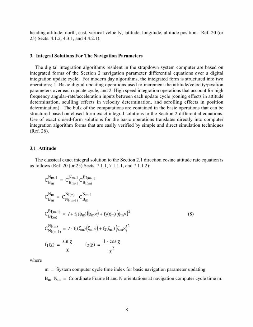
3.1 Attitude

The classical exact integral solution to the Section 2.1 direction cosine attitude rate equation isas follows (Ref. 20 (or 25) Sects. 7.1.1, 7.1.1.1, and 7.1.1.2):

CBm

Nm-1 = CBm-1

Nm-1 CBI(m)

BI(m-1)

CBm

Nm = CNI(m-1)

NI(m) CBm

Nm-1

CBI(m)

BI(m-1) = I + f1(φm) φm× + f2(φm) φm× 2

(8)

CNI(m-1)

NI(m) = I - f1(ζm) ζm× + f2(ζm) ζm× 2

f1 (χ) ≡ sin χ

χ f2 (χ) ≡

1 - cos χ

χ2

where

m = System computer cycle time index for basic navigation parameter updating.

Bm, Nm = Coordinate Frame B and N orientations at navigation computer cycle time m.

8

BI(m) , NI(m) = Discrete orientation of the B and N Frames in non-rotating inertial space

(I) at computer cycle time tm.

I = Identity matrix.

φm, ζm = Rotation vector equivalents to the CBI(m)

BI(m-1) and CNI(m-1)

NI(m) direction cosine

matrices (See Reference 20 (or 25) Section 3.2.2 for rotation vectordefinition).

φm, ζm = Magnitudes of φm, ζm.

χ = Dummy angle parameter.

Reference 20 (or 25) Sections 7.1.2, 7.1.2.1 and 7.1.2.2 provide the equivalent quaternion

formulation integral solution which also is a function of the identical φm, ζm rotation vectors.

Under constant inertial angular rates of the B and N Frames (ωIBB

and ωINN

), the φm, ζm rotation

vectors equal the simple integral of the B and N Frame inertial angular rates over the tm-1 to tm

time interval. Under dynamic angular rate conditions, φm, ζm contain small additional "coning"

terms that account for dynamic variations. The computation of φm and ζm is discussed in

Section 3.4.

All of Equations (8) are analytically exact under general dynamic angular-rate conditions. Animportant point to recognize is that both direction cosine and quaternion based attitude

algorithms have exact solutions using the identical φm, ζm rotation vector inputs. Hence,

contrary to outdated popular belief, modern day quaternion and direction cosine attitudealgorithm formulations have equal accuracy.

3.2 Velocity

The velocity algorithm implemented in the navigation software can be formulated from theintegral of Equation (6) using a trapezoidal integration approximation for the small and/or slowlyvarying terms (Ref. 20 (or 25) Sects. 7.2, 7.2.2, 7.2.2.2 and 7.2.2.2.1 - note correction toEquation (7.2.2-4)):

vmN

= vm-1N

+ ΔvSFm

N + ΔvG/CORm

N

ΔvG/CORm

N = vG/COR

.N dttm-1

tm

≈ 12

3 vG/CORm-1

.N - vG/CORm-2

.N Tm (9)

(Conntinued)

9

vG/COR

. N ≡ gN - ωIEN

× ωIE N

× RN - ωINN

+ ωIEN

× vN

ΔvSFm

N =

12

CNI(m-1)

NI(m) + I ΔvSFm

Nm-1 ≈

12

2 CNI(m-2)

NI(m-1) - CNI(m-3)

NI(m-2) + I ΔvSFm

Nm-1

ΔvSFm

Nm-1 = CBm-1

Nm-1 ΔvSFm

Bm-1(9) (Continued)

ΔvSFm

Bm-1 = CBI (t)

BI(m-1) aSFB

dttm-1

tm

= I + f2(φm) φm× + f3(φm) φm× 2

ηm

CBI (t)BI(m-1) = I + CBI (t)

BI(m-1) ωIBB

× dτtm-1

t

f3 (χ) ≡ 1

χ2 1 -

sin χ

χ

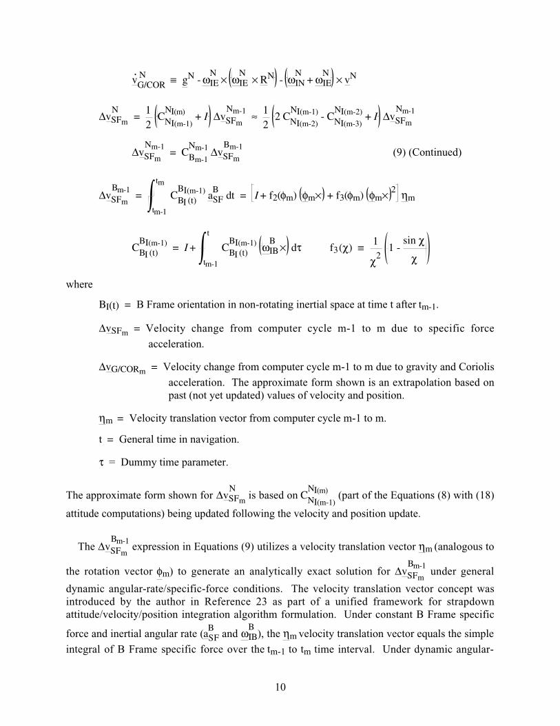
where

BI(t) = B Frame orientation in non-rotating inertial space at time t after tm-1.

ΔvSFm = Velocity change from computer cycle m-1 to m due to specific force

acceleration.

ΔvG/CORm = Velocity change from computer cycle m-1 to m due to gravity and Coriolis

acceleration. The approximate form shown is an extrapolation based onpast (not yet updated) values of velocity and position.

ηm = Velocity translation vector from computer cycle m-1 to m.

t = General time in navigation.

τ = Dummy time parameter.

The approximate form shown for ΔvSFm

N is based on CNI(m-1)

NI(m) (part of the Equations (8) with (18)

attitude computations) being updated following the velocity and position update.

The ΔvSFm

Bm-1 expression in Equations (9) utilizes a velocity translation vector ηm (analogous to

the rotation vector φm) to generate an analytically exact solution for ΔvSFm

Bm-1 under general

dynamic angular-rate/specific-force conditions. The velocity translation vector concept wasintroduced by the author in Reference 23 as part of a unified framework for strapdownattitude/velocity/position integration algorithm formulation. Under constant B Frame specific

force and inertial angular rate (aSFB

and ωIBB

), the ηm velocity translation vector equals the simple

integral of B Frame specific force over the tm-1 to tm time interval. Under dynamic angular-

10

rate/specific-force conditions, ηm contains a small additional "sculling" term that accounts for

dynamic variations. The computation of ηm is discussed in Section 3.4.

Except for trapezoidal integration error in the small and/or slowly varying terms, all ofEquations (9) are analytically exact under general dynamic angular-rate/specific-forceconditions.

3.3 Position

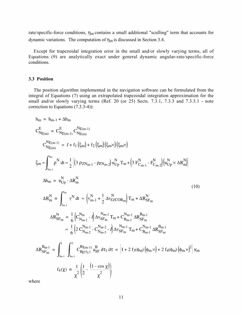
The position algorithm implemented in the navigation software can be formulated from theintegral of Equations (7) using an extrapolated trapezoidal integration approximation for thesmall and/or slowly varying terms (Ref. 20 (or 25) Sects. 7.3.1, 7.3.3 and 7.3.3.1 - notecorrection to Equations (7.3.3-4)):

hm = hm-1 + Δhm

CNE(m)

E = CNE(m-1)

E CNE(m)

NE(m-1)

CNE(m)

NE(m-1) = I + f1 ξm + f2 ξm ξm× ξm×

ξm ≈ ρN dt

tm-1

tm

≈ 12

3 ρZNm-1 - ρZNm-2 uUpN

Tm + 3 FCm-1

N - FCm-2

N uUp

N × ΔRm

N

Δhm = uUpN

⋅ ΔRmN

(10)

ΔRmN

≡ vN dttm-1

tm

≈ vm-1N

+ 12

ΔvG/CORm

N Tm + ΔRSFm

N

ΔRSFm

N =

16

CNm-1

Nm - I ΔvSFm

Nm-1 Tm + CBm-1

Nm-1 ΔRSFm

Bm-1

≈ 16

2 CNm-2

Nm-1 - CNm-3

Nm-2 - I ΔvSFm

Nm-1 Tm + CBm-1

Nm-1 ΔRSFm

Bm-1

ΔRSFm

Bm-1 = tm-1

t

CBI(τ1)BI(m-1) aSF

B dτ1 dτ

tm-1

τ

= I + 2 f3(φm) φm × + 2 f4(φm) φm × 2 κm

f4 (χ) ≡ 1

χ2

12

- 1 - cos χ

χ2

where

11

NE(m) = Discrete orientation of the N Frame in rotating earth space (E) at computer

cycle time tm.

ξm = Rotation vector equivalent to the CNE(m)

NE(m-1) direction cosine matrix. The

computation is an extrapolated trapezoidal approximation to the exact integral of

ξ.

over an m cycle (similar to the Section 3.4 Equation (18) approximation for the

integral of ζ.

in Equation (11), but using ρN in place of ωIN

N).

ξm = Magnitude of ξm.

ζm = Calculated in Section 3.4 Equations (18).

Δhm = Altitude change from computer cycle m-1 to m.

ΔRm = Position vector change from computer cycle m-1 to m.

ΔRSFm = Specific force acceleration contribution to ΔRm.

κm = Position translation vector from cycle m-1 to m.

The ΔRSFm

Bm-1 expression in Equations (10) utilizes a position translation vector κm (analogous

to the rotation vector φm) to generate an analytically exact solution for ΔRSFm

Bm-1 under general

dynamic angular-rate/specific-force conditions. The position translation vector concept wasintroduced by the author in Reference 23 as part of a unified framework for strapdownattitude/velocity/position integration algorithm formulation. Under constant B Frame specific

force and inertial angular rate (aSFB

and ωIBB

), the κm position translation vector equals the simple

double integral of B Frame specific force over the tm-1 to tm time interval. Under dynamic

angular-rate/specific-force conditions, κm contains a small additional "scrolling" term that

accounts for dynamic variations. The computation of κm is discussed in Section 3.4.

Except for trapezoidal integration error in the small and/or slowly varying terms, all ofEquations (10) are analytically exact under general dynamic angular-rate/specific-forceconditions.

3.4 Computing The Rotation And Translation Vectors

The form of the CBI(m)

BI(m-1), CNI(m-1)

NI(m) expressions in (8) can be derived as the exact solution to

Equations (1) under constant B and N Frame inertial angular rate (Ref. 20 (or 25) Sects. 3.2.2and 3.2.2.1). The result would be identical to (8), but with the rotation vectors replaced by the

12

integrals of the B and N Frame inertial rotation rates. Similarly, the forms of the ΔvSFm

Bm-1and

ΔRSFm

Bm-1 expressions in (9) and (10) can be derived as the exact analytic solution to the integrals

in these expressions under constant B Frame inertial angular rate and specific force (Refs. 19 and

20 (or 25) Sects. 7.2.2.2 and 7.3.3). The result would be identical to the ΔvSFm

Bm-1 and ΔRSFm

Bm-1

expressions in (9) and (10), but with the rotation vector replaced by integrated B Frame angularrate and the velocity/position translation vectors replaced by the integral and double integral of B

Frame specific force. In fact, the ΔvSFm

Bm-1 and ΔRSFm

Bm-1 expressions in (9) and (10) were derived in

Reference 23 as the aforementioned exact solution under constant B Frame angular-rate/specific-force solution, but for general motion having the integrated B Frame angular rate term replacedby the rotation vector and the integrated/doubly-integrated B Frame specific force terms replacedby the translation vectors. This is the same approach used by Jordan in Reference 8 for

introducing the CBI(m)

BI(m-1) expression in (8) (which has been extended in this paper to also include

CNI(m-1)

NI(m)). For the Jordan case, the rotation vector was formulated by approximation as integrated

angular rate plus a coning correction based on the Goodman-Robinson theorem (Ref. 4). Therotation vector concept was introduced by Euler and utilized by Laning in 1949 (Ref. 10) todevelop the classical exact rotation vector rate of change equation (shown subsequently in thissection) for strapdown inertial navigation application. Note: In 1971 Bortz reintroduced andapplied the exact Laning rotation vector rate equation in a strapdown system/softwareimplementation (Ref. 1) for which it has since been known as the "Bortz equation".

The integral of the Laning rotation vector rate equation provides an exact solution for the

rotation vector input to the CBI(m)

BI(m-1), CNI(m-1)

NI(m) expressions in (8). Based on the previous

discussion, the velocity/ position translation vectors ηm, κm can be analytically defined as the

vectors that satisfy the ΔvSFm

Bm-1 expression in (9) and the ΔRSFm

Bm-1 expression in (10). Using this

definition, References 23 or 25 (Section 19.1.5) derive analytically exact equations for thetranslation vector rates of change (shown subsequently) which, when integrated from time tm-1 to

tm, provide exact solutions for ηm and κm. References 23, 25 Sect. 19.1, and 20 (or 25) Sect.

7.1.1.2 then show that the following simplified forms can be utilized as accurate approximations

for the φ.

, ζ.

, η.

and κ.

rotation/translation vector rates (Ref. 23 Equations (31) or Ref. 25

Equations (19.1.8-3), and Ref. 20 (or 25) Equation (7.1.1.2-4)):

13

φ.

≈ ωIBB +

12

α(t) × ωIBB α(t) ≡ ωIB

B dτ

tm-1

t

ζ.

≈ ωINN

η.

≈ aSFB +

12

α(t) × aSFB

- ωIBB

× υ(t) υ(t) ≡ aSFB

dτtm-1

t (11)

κ.

= η(t) + 16

α(t) × υ(t) - 2 ωIBB

× Sυ(t) Sυ(t) ≡ υ dτtm-1

t

The error in the Equations (11) approximation is minimized by using a small value for the

computer update cycle time interval tm-1 to tm, thereby assuring small values of φ and ζ. Using

Equations (1) for ωINN

with a trapezoidal integration algorithm (Ref. 20 (or 25) Sect. 7.1.1.2.1),

the integral of Equations (11) over a computer update cycle then becomes for therotation/translation vector inputs to Equations (8), (9) and (10):

φm = αm + ΔφConem ηm = υm + ΔηSculm

κm = Sυm + ΔκScrlm (12)

ΔφConem = 12

α t × ωIBB

dttm-1

tm

Coning (13)

ΔηScul(t) = 12

α(τ) × aSFB

+ υ(τ) × ωIBB

dτtm-1

t

ΔηSculm = ΔηScul(tm)

Sculling (14)

ΔκScrlm = 16

6 ΔηScul(t) + α(t) × υ(t) - 2 ωIBB

× Sυ(t) dttm-1

tm

Scrolling (15)

Sυ(t) = υ(τ) dτtm-1

t

Sυm = Sυ(tm)Doubly integrated

specifice force acceleration(16)

14

α(t) = ωIBB

dτtm-1

t

υ(t) = aSFB

dτtm-1

t

αm = α(tm) υm = υ(tm)

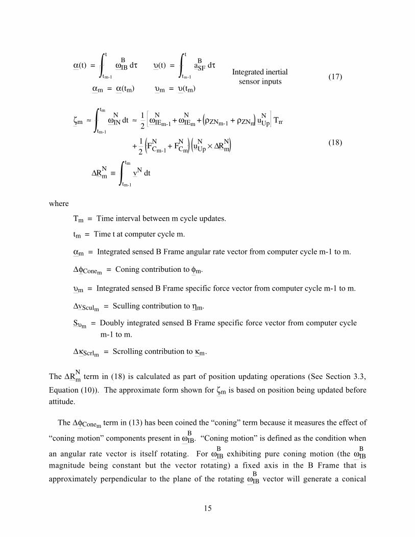
Integrated inertialsensor inputs

(17)

ζm ≈ ωINN

dttm-1

tm

≈ 12

ωIEm-1

N + ωIEm

N + ρZNm-1 + ρZNm uUp

N Tm

+ 12

FCm-1

N + FCm

N uUp

N × ΔRm

N

ΔRmN

≡ vN dttm-1

tm

(18)

where

Tm = Time interval between m cycle updates.

tm = Time t at computer cycle m.

αm = Integrated sensed B Frame angular rate vector from computer cycle m-1 to m.

ΔφConem = Coning contribution to φm.

υm = Integrated sensed B Frame specific force vector from computer cycle m-1 to m.

ΔvSculm = Sculling contribution to ηm.

Sυm = Doubly integrated sensed B Frame specific force vector from computer cycle

m-1 to m.

ΔκScrlm = Scrolling contribution to κm.

The ΔRmN

term in (18) is calculated as part of position updating operations (See Section 3.3,

Equation (10)). The approximate form shown for ζm is based on position being updated before

attitude.

The ΔφConem term in (13) has been coined the “coning” term because it measures the effect of

“coning motion” components present in ωIBB

. “Coning motion” is defined as the condition when

an angular rate vector is itself rotating. For ωIBB

exhibiting pure coning motion (the ωIBB

magnitude being constant but the vector rotating) a fixed axis in the B Frame that is

approximately perpendicular to the plane of the rotating ωIBB

vector will generate a conical

15

surface in the I Frame as the angular rate motion ensues (hence, the term “coning” to describe the

motion). Under coning angular motion conditions, B Frame axes perpendicular to ωIBB

appear to

oscillate (in contrast with non-coning or “spinning” angular motion in which axes perpendicular

to ωIBB

rotate around ωIBB

). Note that the neglected terms in the ζ equation can also be identified

as coning associated with the ωINN

rate vector.

The ΔηSculm term in Equations (14), denoted as “sculling”, measures the “constant”

contribution to ηm created by combined dynamic angular-rate/specific-force rectification. The

rectification is a maximum under classical sculling motion defined as sinusoidal angular-

rate/specific-force in which the α(t) angular excursion about one B Frame axis is at the same

frequency and in phase with the aSFB

specific force along another B Frame axis (with a constant

acceleration component then produced along the average third axis direction). This is the sameprinciple used by mariners to propel a boat in the forward direction using a single oar operatedwith an undulating motion (also denoted as “sculling", the original use of the term).

The Δκ Scrlm term in (15), denoted as “scrolling”, is analogous to sculling in the velocity

translation vector update equations. It measures the “constant” contribution to κm created by

combined dynamic angular-rate/specific-force rectification. (The term “scrolling” was coined bythe author merely to have a name for the term and also to have one that sounds like “sculling”,but for position integration - change in the position vector R stressing the “R” sound. Thecomplex mathematical formulations that accompany “scrolling” may be a more appropriate

reason for the name). For all but the most exacting positioning applications, ΔRScrlm can be

safely neglected.

Equations (11) (the basis for Equations (12) - (18)) are approximate forms of the followingexact rotation/translation vector rate equations (Ref. 10, Ref. 20 (and 25) Sect. 7.1.1.1, Ref. 23,Equations (15) - (16) and Ref. 25 Sect. 19.1.5):

φ.

= ωIBB

+ 12

φ × ωIBB

+ f5(φ) φ × φ × ωIBB

ζ.

= ωINN

+ 12

ζ × ωINN

+ f5(ζ) ζ × ζ × ωINN

η.

= aSFB

+ 12

φ × aSF - φ.

× η + f5(φ) φ × φ × aSFB

- φ.

× η + f3(φ) φ × φ.

× η

+ 12

f3(φ) φ × φ × φ.

× η - φ ⋅ η φ × φ.

+ f6(φ) φ ⋅ φ.

× η φ - f7(φ) φ ⋅ η φ × φ × φ.

(19)

κ.

= η + 16

φ × η - 2 φ.

× κ + f8(φ) φ × φ × η - 2 φ.

× κ + 2 f4(φ) φ × φ.

× κ

- f9(φ) φ × φ × φ.

× κ - f10(φ) φ2 φ × η - 2 φ

. × κ + f11(φ) φ ⋅ φ

. × κ φ

+ f12(φ) φ × φ × φ.

× κ - f13(φ) φ ⋅ κ φ × φ × φ.

16

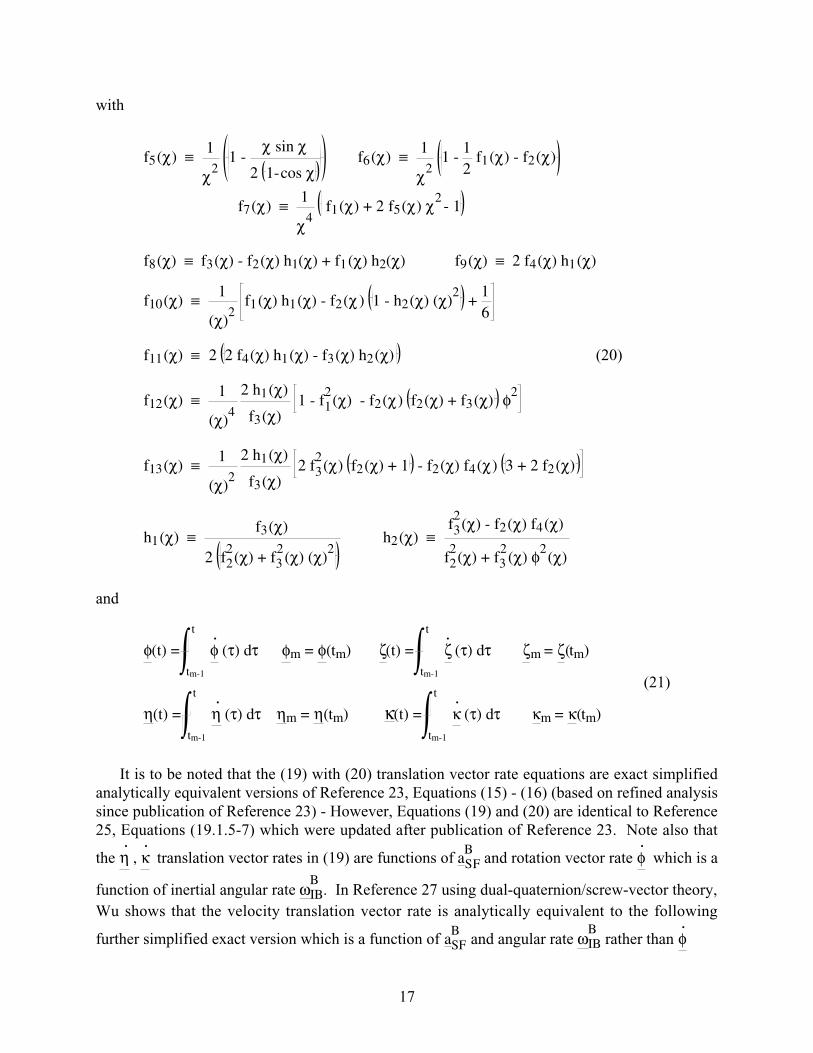
with

f5 (χ) ≡ 1

χ2 1 -

χ sin χ

2 1- cos χ f6 (χ) ≡

1

χ2 1 -

12

f1 (χ) - f2 (χ)

f7 (χ) ≡ 1

χ4 f1 (χ) + 2 f5 (χ) χ2

- 1

f8 (χ) ≡ f3 (χ) - f2 (χ) h1(χ) + f1 (χ) h2(χ) f9 (χ) ≡ 2 f4 (χ) h1 (χ)

f10 (χ) ≡ 1

(χ)2

f1 (χ) h1 (χ) - f2 (χ ) 1 - h2 (χ) (χ)2

+ 16

f11 (χ) ≡ 2 2 f4 (χ) h1 (χ) - f3 (χ) h2 (χ) (20)

f12 (χ) ≡ 1

(χ)4

2 h1 (χ)

f3 (χ) 1 - f1

2 (χ) - f2 (χ) f2 (χ) + f3 (χ) φ2

f13 (χ) ≡ 1

(χ)2

2 h1 (χ)

f3 (χ) 2 f3

2 (χ) f2 (χ) + 1 - f2 (χ) f4 (χ) 3 + 2 f2 (χ)

h1 (χ) ≡ f3 (χ)

2 f22

(χ) + f32

(χ) (χ)2

h2 (χ) ≡ f32

(χ) - f2 (χ) f4 (χ)

f22

(χ) + f32

(χ) φ2 (χ)

and

φ(t) = φ.

(τ) dτtm-1

t

φm = φ(tm) ζ(t) = ζ.

(τ) dτtm-1

t

ζm = ζ(tm)

η(t) = η.

(τ) dτtm-1

t

ηm = η(tm) κ(t) = κ.

(τ) dτtm-1

t

κm = κ(tm)

(21)

It is to be noted that the (19) with (20) translation vector rate equations are exact simplifiedanalytically equivalent versions of Reference 23, Equations (15) - (16) (based on refined analysissince publication of Reference 23) - However, Equations (19) and (20) are identical to Reference25, Equations (19.1.5-7) which were updated after publication of Reference 23. Note also that

the η.

, κ.

translation vector rates in (19) are functions of aSFB

and rotation vector rate φ.

which is a

function of inertial angular rate ωIBB

. In Reference 27 using dual-quaternion/screw-vector theory,

Wu shows that the velocity translation vector rate is analytically equivalent to the following

further simplified exact version which is a function of aSFB

and angular rate ωIBB

rather than φ.

17

η.

= aSFB

+ 12

φ × aSF - ωIBB

× η + f5 (φ) φ × φ × aSFB

- ωIBB

× η - φ × ωIBB

× η

+ f14 (φ) φ ⋅ η φ × φ × ωIBB

with (22)

f14 (χ) ≡ χ + sin χ

2 χ3 1 - cos χ

- 2

χ4

As of this writing, a further simplified version of the exact position translation vector rateequation in (19) has yet to be found (Ref. 24).

Equations (19) - (22) are analytically exact under general angular-rate/specific-force dynamicconditions. It is easily verified by inspection that under constant B and N Frame inertial angularrate and constant B Frame specific force, the rotation/translation vectors reduce identically to the

integrals of the first term in their respective rate equations (i.e., integrated ωIBB

, ωINN

for φ, ζ,

integrated aSFB

for η, and doubly integrated aSFB

for κ), as they should in light of the discussion at

the beginning of this section on their derivation. The additional terms in these equations (i.e.,coning, sculling and scrolling) are small contributions excited by dynamic high frequency inputs(e.g., vibration), and not by lower frequency dynamic inputs that impact the leading terms. Forexample, in a 7.6 g root-mean-square aircraft vibration environment, Reference 20 (or 25),Section 7.4 shows that coning/sculling rates on the sensor assembly could be 9.9 deg/hr and 1.3milli-gs worst case for a typically mounted INS (compared to lower frequency dynamicmaneuver angular-rates/accelerations (e.g., 200 deg/sec and 10 gs) impacting the leading terms).Because the coning/sculling/scrolling terms are small, they can be accurately approximated bysimplified versions of these terms in Equations (19) - (20). The principal benefit afforded by theuse of rotation/translation vectors in structuring general strapdown navigation equations is thattheir rate equations can thereby be drastically simplified with virtually negligible error (Ref. 23).The utility of the exact rotation/translation rate representations in (19) - (22) is to provide a validexact base from which to formulate simplified versions (e.g., Equations (11)) used forsubsequent algorithm development, and as a reference for accuracy assessment of the simplifiedversions (Ref. 23).

3.5 Summary of Main Terms Requiring Integration Algorithms

Equations (8), (9) and (10) with (12) - (18) are integral solutions to Equations (3), (6) and (7)over a computer update cycle. For the most part, they consist of exact closed form expressions

fed by the integrated sensor output terms in Equations (13) - (17). The α, υ integrated angular

rate and specific force acceleration signals in (17) (measured by summing (integrating) angularrate sensor and accelerometer integrated output increments) are the normal basic inputs to moststrapdown inertial system algorithms. The Equations (13) - (16) terms (coning, sculling,scrolling, doubly integrated accelerometer signals) represent functions to be implemented byhigh speed digital computation algorithms operating within the basic m cycle update period.

18

4. DIGITAL INTEGRATION ALGORITHMS

Digital algorithms in the strapdown system computer are structured to provide integralsolutions to the Section 2 differential equations based on repetitive processing at a specifiedcomputation rate. The integral solutions in Section 3 to the Section 2 equations have such arepetitive processing structure, hence, for the most part, are the digital algorithm forms to beprogrammed directly in the strapdown computer. These are exact solution forms, hence, have noalgorithm error if programmed as shown (except for minor trapezoidal integration algorithmerrors for the small/slowly varying terms). Exceptions are the coning, sculling, scrolling anddoubly integrated sensor signal integrals in Section 3.4, Equations (13 - (16) needing high speeddigital integration algorithms for implementation. The high speed algorithm errors are a functionof the high speed digital integration update frequency. Additionally, Taylor series expansionalgorithms are needed for the trigonometric function coefficients in Equations (8), (9) and (10)

that avoid singularities when φm or ζm are near zero. Taylor series truncation error can be

designed to be negligible by carrying sufficient terms.

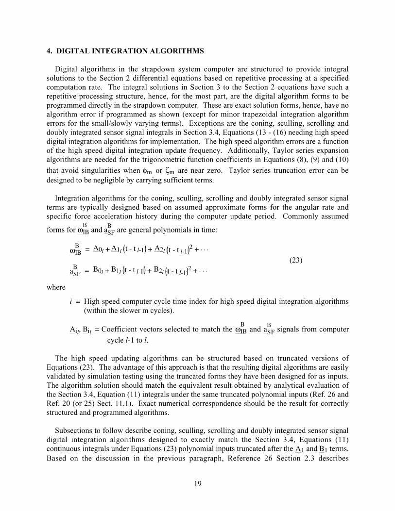
Integration algorithms for the coning, sculling, scrolling and doubly integrated sensor signalterms are typically designed based on assumed approximate forms for the angular rate andspecific force acceleration history during the computer update period. Commonly assumed

forms for ωIBB

and aSFB

are general polynomials in time:

ωIBB = A0l + A1l t - t l-1 + A2l t - t l-1

2 +

aSFB = B0l + B1l t - t l-1 + B2l t - t l-1

2 + (23)

where

l = High speed computer cycle time index for high speed digital integration algorithms(within the slower m cycles).

Ail, Bil = Coefficient vectors selected to match the ωIBB

and aSFB

signals from computer

cycle l-1 to l.

The high speed updating algorithms can be structured based on truncated versions ofEquations (23). The advantage of this approach is that the resulting digital algorithms are easilyvalidated by simulation testing using the truncated forms they have been designed for as inputs.The algorithm solution should match the equivalent result obtained by analytical evaluation ofthe Section 3.4, Equation (11) integrals under the same truncated polynomial inputs (Ref. 26 andRef. 20 (or 25) Sect. 11.1). Exact numerical correspondence should be the result for correctlystructured and programmed algorithms.

Subsections to follow describe coning, sculling, scrolling and doubly integrated sensor signaldigital integration algorithms designed to exactly match the Section 3.4, Equations (11)continuous integrals under Equations (23) polynomial inputs truncated after the A1 and B1 terms.

Based on the discussion in the previous paragraph, Reference 26 Section 2.3 describes

19

specialized simulators for validating algorithms of this structure. Following subsections also

discuss singularity free algorithms for computing the f1 (χ) - f4 (χ) trigonometric functions in

Sections 3.1-3.3 and whether orthogonality/normalization corrections are needed for the attitudealgorithms.

4.1 Coning Digital Integration Algorithm

A coning digital computation algorithm for Equation (13) is given by (Ref. 20 (or 25) Sect.7.1.1.1.1):

ΔφConem = 12

αl-1 + 16

Δαl-1 × Δαl∑l

From tm-1 to tm

αl = Δαl∑l

From tm-1 to tl Δαl = dαt l-1

t l(24)

where

Δαl = Summation of integrated angular rate sensor output increments from cycle l-1 to

l.

Equations (24) have been designed to be exact under Equations (23) angular rate input with

the ωIBB

polynomial truncated after the A1 term.

4.2 Sculling Digital Integration Algorithm

A sculling digital computation algorithm for Equation (14) is given by (Ref. 20 (or 25) Sect.7.2.2.2.2):

ΔηSculm = ΔηScull At tm

ΔηScull = 12

α l-1 + 16

Δαl-1 × Δυ l + υ l-1 + 16

Δυl-1 × Δα l∑l

From tm-1 to tl (25)

υl = Δυl∑l

From tm-1 to tl Δυl = dυt l-1

t l

where

Δυl = Summation of integrated accelerometer output increments from cycle l-1 to l.

20

Equations (25) have been designed to be exact under Equations (23) angular rate and specific

force inputs with the ωIBB

, aSFB

polynomials truncated after the A1, B1 terms.

Note the similarity in form between the Equations (24) coning algorithm and Equations (25)sculling algorithm. Reference 14 provides a general formula for deriving the equivalent scullingalgorithm (e.g., Equations (25)) from a previously derived coning algorithm (e.g., Equations(24)).

4.3 Scrolling And Doubly Integrated Sensor Signal Algorithms

Digital algorithms for scrolling computation and doubly integrated sensor signals forEquations (15) - (16) are given by Reference 25, Equations (19.1.11-1) (based on a similardevelopment in Ref. 20 (or 25) Sect. 7.3.3.2 for an alternative scrolling formula):

ΔκScrlm = δκScrlAl + δκScrlBl∑l

From tm-1 to tm

δκScrlAl = ΔηScull-1 Tl + 12

αl-1 - 112

Δαl - Δαl-1 × ΔSυl - υl-1 Tl

+ 12

υl-1 - 112

Δυl - Δυl-1 × ΔSαl - αl-1 Tl

ΔδζScrlBl = 13

Sυl-1 - 18

Δυl Tl × Δαl

+ 16

αl-1 - 34

Δαl + 14

Δαl-1 × υl-1 + 512

Δυl + 112

Δυl-1 Tl

+ 1

1440 Δαl - Δαl-1 × Δυl - Δυl-1 Tl

(26)

ΔSαl = αl-1Tl + Tl

12 5 Δαl + Δ αl-1 ΔSυl = υl-1Tl +

Tl

12 5 Δυl + Δυl-1

Sυl = ΔSυl∑l

From tm-1 to tl Sυm = Sυl at tm

where

Tl = Time interval between computer high speed l cycles.

Equations (26) have been designed to be exact under Equations (23) angular rate and specific

force inputs with the ωIBB

, aSFB

polynomials truncated after the A1, B1 terms.

21

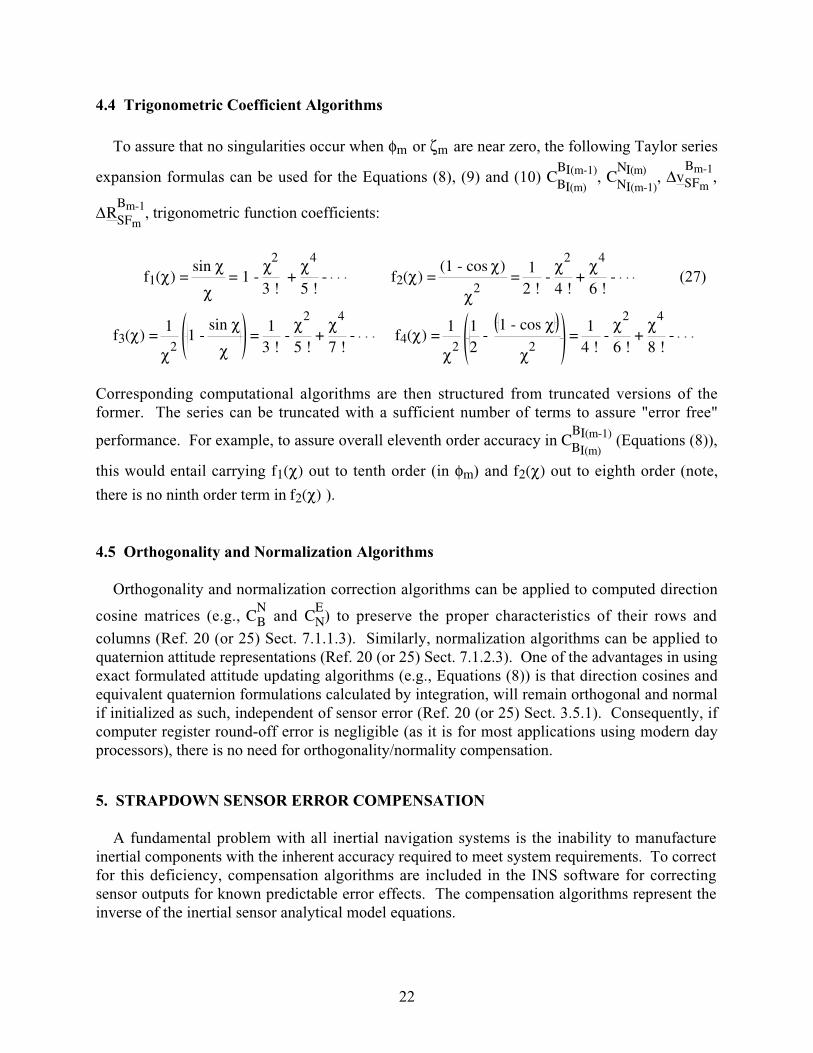
4.4 Trigonometric Coefficient Algorithms

To assure that no singularities occur when φm or ζm are near zero, the following Taylor series

expansion formulas can be used for the Equations (8), (9) and (10) CBI(m)

BI(m-1), CNI(m-1)

NI(m), ΔvSFm

Bm-1,

ΔRSFm

Bm-1, trigonometric function coefficients:

f1 (χ) = sin χ

χ = 1 -

χ2

3 ! +

χ4

5 ! - f2 (χ) =

(1 - cos χ)

χ2 =

12 !

- χ2

4 ! +

χ4

6 ! - (27)

f3 (χ) = 1

χ2 1 -

sin χ

χ =

13 !

- χ2

5 ! +

χ4

7 ! - f4 (χ) =

1

χ2

12

- 1 - cos χ

χ2 =

14 !

- χ2

6 ! +

χ4

8 ! -

Corresponding computational algorithms are then structured from truncated versions of theformer. The series can be truncated with a sufficient number of terms to assure "error free"

performance. For example, to assure overall eleventh order accuracy in CBI(m)

BI(m-1) (Equations (8)),

this would entail carrying f1(χ) out to tenth order (in φm) and f2(χ) out to eighth order (note,

there is no ninth order term in f2(χ) ).

4.5 Orthogonality and Normalization Algorithms

Orthogonality and normalization correction algorithms can be applied to computed direction

cosine matrices (e.g., CBN

and CNE

) to preserve the proper characteristics of their rows and

columns (Ref. 20 (or 25) Sect. 7.1.1.3). Similarly, normalization algorithms can be applied toquaternion attitude representations (Ref. 20 (or 25) Sect. 7.1.2.3). One of the advantages in usingexact formulated attitude updating algorithms (e.g., Equations (8)) is that direction cosines andequivalent quaternion formulations calculated by integration, will remain orthogonal and normalif initialized as such, independent of sensor error (Ref. 20 (or 25) Sect. 3.5.1). Consequently, ifcomputer register round-off error is negligible (as it is for most applications using modern dayprocessors), there is no need for orthogonality/normality compensation.

5. STRAPDOWN SENSOR ERROR COMPENSATION

A fundamental problem with all inertial navigation systems is the inability to manufactureinertial components with the inherent accuracy required to meet system requirements. To correctfor this deficiency, compensation algorithms are included in the INS software for correctingsensor outputs for known predictable error effects. The compensation algorithms represent theinverse of the inertial sensor analytical model equations.

22

This section describes error models and compensation algorithms that can be used to correctfor errors in the strapdown inertial sensors (angular rate sensors and accelerometers), relativedisplacement between accelerometers (“size effect”), misalignment of the strapdown sensorassembly relative to the system mount, and alignment of the system mount in the user vehiclerelative to vehicle reference axes. Included is a discussion of the application of the sensorcompensation algorithms to the Section 4 strapdown inertial navigation integration routines andtheir associated coning, sculling, scrolling and accelerometer size-effect/anisoinertia elements.

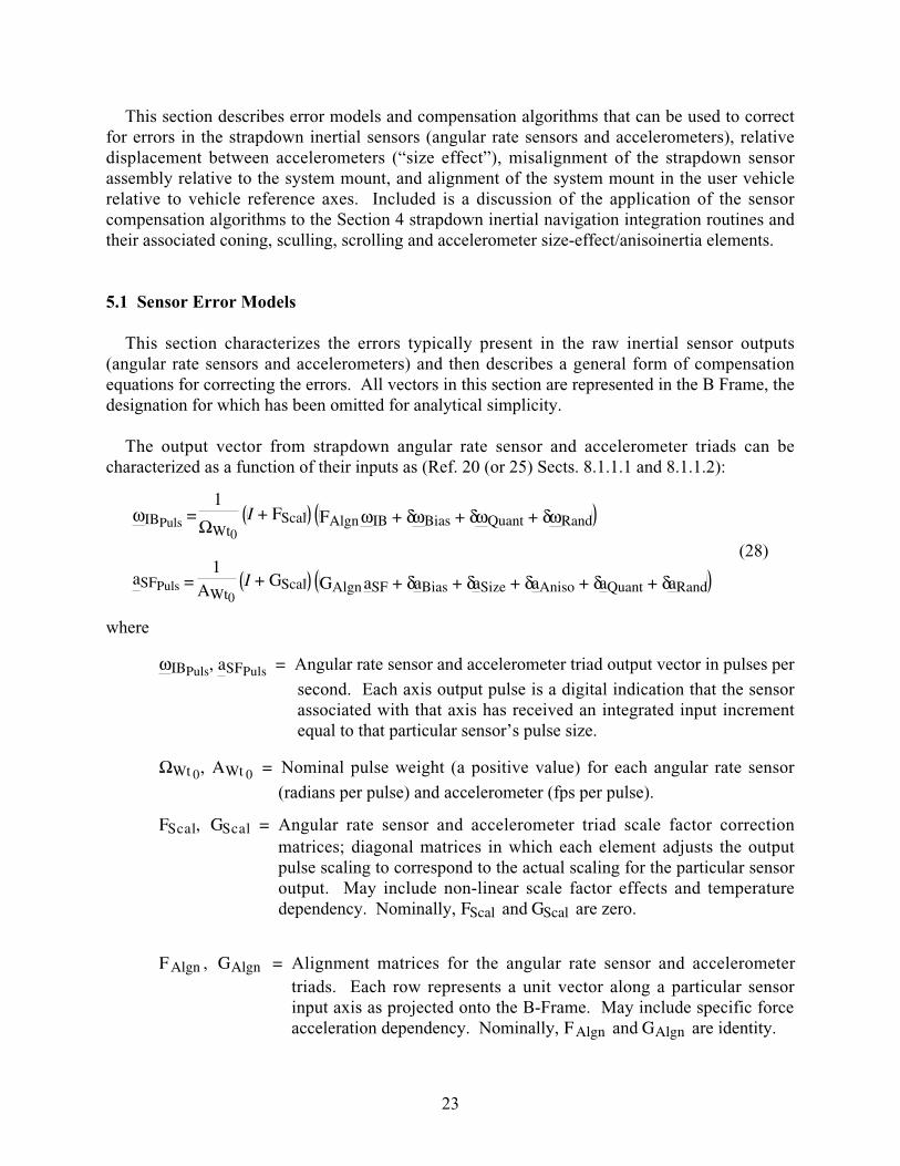
5.1 Sensor Error Models

This section characterizes the errors typically present in the raw inertial sensor outputs(angular rate sensors and accelerometers) and then describes a general form of compensationequations for correcting the errors. All vectors in this section are represented in the B Frame, thedesignation for which has been omitted for analytical simplicity.

The output vector from strapdown angular rate sensor and accelerometer triads can becharacterized as a function of their inputs as (Ref. 20 (or 25) Sects. 8.1.1.1 and 8.1.1.2):

ωIBPuls = 1

ΩWt0 I + FScal FAlgn ωIB + δωBias + δωQuant + δωRand

aSFPuls = 1

AWt0 I + GScal GAlgn aSF + δaBias + δaSize + δaAniso + δaQuant + δaRand

(28)

where

ωIBPuls, aSFPuls = Angular rate sensor and accelerometer triad output vector in pulses per

second. Each axis output pulse is a digital indication that the sensorassociated with that axis has received an integrated input incrementequal to that particular sensor’s pulse size.

ΩWt 0, AWt 0 = Nominal pulse weight (a positive value) for each angular rate sensor

(radians per pulse) and accelerometer (fps per pulse).

FScal, GScal = Angular rate sensor and accelerometer triad scale factor correction

matrices; diagonal matrices in which each element adjusts the outputpulse scaling to correspond to the actual scaling for the particular sensoroutput. May include non-linear scale factor effects and temperaturedependency. Nominally, FScal and GScal are zero.

FAlgn , GAlgn = Alignment matrices for the angular rate sensor and accelerometer

triads. Each row represents a unit vector along a particular sensorinput axis as projected onto the B-Frame. May include specific forceacceleration dependency. Nominally, FAlgn and GAlgn are identity.

23

δωBias, δ aBias = Angular rate sensor and accelerometer triad bias vectors. Each

element equals the systematic output from a sensor under zero inputconditions. May have environmental sensitivities (e.g., temperature,specific force acceleration for angular rate sensors, angular rate foraccelerometers).

δωQuant, δaQuant = Instantaneous angular rate sensor and accelerometer triad pulse

quantization error vectors associated with the output only beingprovided when the cumulative input equals the pulse weight peraxis.

δωRand, δaRand = Angular rate sensor and accelerometer triad random error output

vectors.

δ aSize = Accelerometer triad size effect error created by the fact that due to physical

size, the accelerometers in the triad cannot be collocated, hence, do notmeasure components of identically the same acceleration vector.

δaAniso = Accelerometer triad anisoinertia error effect (present in pendulous

accelerometers) created by mismatch in the moments of inertia around theinput and pendulum axes.

References 21 and 20 (or 25) Section 8.1.3 analytically describe the Equations (28) δωQuant,

δaQuant quantization error effects in strapdown inertial sensors. The δaSize size effect term (Ref.

20 (or 25) Sect. 8.1.4.1) and for pendulous accelerometers, the δaAniso anisoinertia term (Ref. 16

and Ref. 20 (or 25) Sect. 8.1.4.2), are given by :

δ aSize ≡ GAlgnk

T ⋅ ωIB

. B × l k + ωIB × ωIB × l k uk∑k=1,3

δaAniso = KAniso ωIBk ωIBkp uk∑k=1,3

(29)

where

uk = Unit vector parallel to the accelerometer k input axis.

l k = Position vector from INS navigation center to accelerometer k center of seismic

mass.

GAlgnk

T = Vector formed from the kth column of GAlgn

T, the transpose of the GAlgn

accelerometer triad alignment matrix.

KAniso = Accelerometer anisoinertia coefficient (a generic property of the accelerometer

design).

24

ωIBk, ωIBkp = Angular rate ωIB projections on the accelerometer k input and kp

pendulum axes.

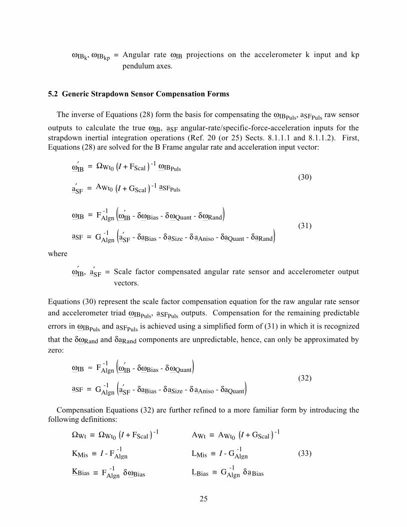
5.2 Generic Strapdown Sensor Compensation Forms

The inverse of Equations (28) form the basis for compensating the ωIBPuls, aSFPuls raw sensor

outputs to calculate the true ωIB, aSF angular-rate/specific-force-acceleration inputs for the

strapdown inertial integration operations (Ref. 20 (or 25) Sects. 8.1.1.1 and 8.1.1.2). First,Equations (28) are solved for the B Frame angular rate and acceleration input vector:

ωIB′ = ΩWt0 I + FScal

-1 ωIBPuls

aSF′ = AWt0 I + GScal

-1 aSFPuls

(30)

ωIB = FAlgn -1 ωIB

′ - δωBias - δωQuant - δωRand

aSF = GAlgn -1 aSF

′ - δaBias - δaSize - δ aAniso - δaQuant - δaRand

(31)

where

ωIB′ , aSF

′ = Scale factor compensated angular rate sensor and accelerometer output

vectors.

Equations (30) represent the scale factor compensation equation for the raw angular rate sensor

and accelerometer triad ωIBPuls, aSFPuls outputs. Compensation for the remaining predictable

errors in ωIBPuls and aSFPuls is achieved using a simplified form of (31) in which it is recognized

that the δωRand and δaRand components are unpredictable, hence, can only be approximated by

zero:

ωIB ≈ FAlgn -1 ωIB

′ - δωBias - δωQuant

aSF = GAlgn -1 aSF

′ - δaBias - δaSize - δ aAniso - δaQuant

(32)

Compensation Equations (32) are further refined to a more familiar form by introducing thefollowing definitions:

ΩWt ≡ ΩWt0 I + FScal -1 AWt ≡ AWt0 I + GScal

-1

KMis ≡ I - FAlgn -1

LMis ≡ I - GAlgn -1

(33)

KBias ≡ FAlgn -1 δ ωBias LBias ≡ GAlgn

-1 δ a Bias

25

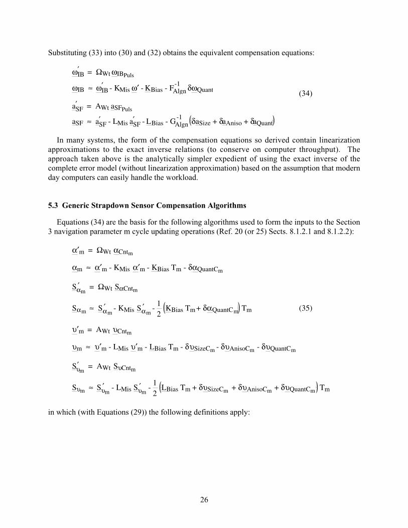
Substituting (33) into (30) and (32) obtains the equivalent compensation equations:

ωIB′ = ΩWt ωIBPuls

ωIB ≈ ωIB′ - KMis ω′ - KBias - FAlgn

-1 δωQuant

(34)

aSF′ = AWt aSFPuls

aSF ≈ aSF′ - LMis aSF

′ - LBias - GAlgn -1

δaSize + δaAniso + δaQuant

In many systems, the form of the compensation equations so derived contain linearizationapproximations to the exact inverse relations (to conserve on computer throughput). Theapproach taken above is the analytically simpler expedient of using the exact inverse of thecomplete error model (without linearization approximation) based on the assumption that modernday computers can easily handle the workload.

5.3 Generic Strapdown Sensor Compensation Algorithms

Equations (34) are the basis for the following algorithms used to form the inputs to the Section3 navigation parameter m cycle updating operations (Ref. 20 (or 25) Sects. 8.1.2.1 and 8.1.2.2):

α′m = ΩWt αCntm

αm ≈ α′m - KMis α′m - KBias Tm - δαQuantCm

Sαm

′ = ΩWt SαCntm

Sαm ≈ Sαm

′ - KMis Sαm

′ - 12

KBias Tm + δαQuantCm Tm (35)

υ′m = AWt υCntm

υm ≈ υ′m - LMis υ′m - LBias Tm - δ υSizeCm - δ υAnisoCm - δ υQuantC m

Sυm

′ = AWt SυCntm

Sυm ≈ Sυm

′ - LMis Sυm

′ - 12

LBias Tm + δυSizeCm + δυAnisoCm + δυQuantCm Tm

in which (with Equations (29)) the following definitions apply:

26

δυSizeCm ≡ GAlgn -1

δ aSize dttm-1

tm

≈ δ aSize dttm-1

tm

= uk ⋅ ωIB.

× l k + ωIB × ωIB × l k uk dt

tm-1

tm

∑k

δυAnisoCm ≡ GAlgn -1

δ aAniso dttm-1

tm

≈ δ aAniso dttm-1

tm

= KAniso uk ωIBk ωIBkp dttm-1

tm

∑k=1,3

(36)

δαQuantCm ≡ FAlgn -1

δωQuant dttm-1

tm

≈ δωQuant dttm-1

tm

δ υQuantC m ≡ GAlgn -1

δaQuant dttm-1

tm

≈ δaQuant dttm-1

tm

αCntm ≡ dαCnttm-1

tm

υCntm ≡ dυCnttm-1

tm Summation of rawsensor output pulses

over computer cycle m

where

dαCnt, dυCnt = Angular rate sensor and accelerometer instantaneous pulse output

vectors.

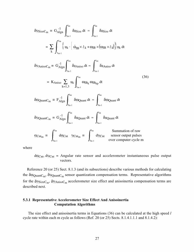
Reference 20 (or 25) Sect. 8.1.3 (and its subsections) describe various methods for calculating

the δαQuantCm, δ υQuantC m sensor quantization compensation terms. Representative algorithms

for the δ υSizeCm, δ υAnisoCm accelerometer size effect and anisoinertia compensation terms are

described next.

5.3.1 Representative Accelerometer Size Effect And AnisoinertiaComputation Algorithms

The size effect and anisoinertia terms in Equations (36) can be calculated at the high speed lcycle rate within each m cycle as follows (Ref. 20 (or 25) Sects. 8.1.4.1.1.1 and 8.1.4.2):

27

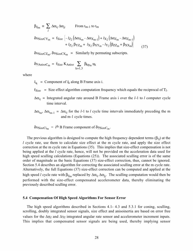
βijm ≡ Δαil Δαjl∑l

From tm-1 to tm

δυSizeCYm = fSize - lZ2 ΔαXm - ΔαXm-1 + lX2 ΔαZm - ΔαZm-1

+ lZ2 βYZm + lX2 βXYm - lY2 βZZm + βXXm

δυSizeCZm, δυSizeCXm = Similarly by permuting subscripts.

(37)

δυAnisoCm = fSize KAniso βkpm uk∑k=1,3

where

lik = Component of lk along B Frame axis i.

fSize = Size effect algorithm computation frequency which equals the reciprocal of Tl.

Δαil = Integrated angular rate around B Frame axis i over the l-1 to l computer cycle

time interval.

Δαim, Δαim-1 = Δαil for the l-1 to l cycle time intervals immediately preceding the m

and m-1 cycle times.

δυSizeCim = ith B Frame component of δυSizeCm .

The previous algorithm is designed to compute the high frequency dependent terms (βij) at the

l cycle rate, use them to calculate size effect at the m cycle rate, and apply the size effectcorrection at the m cycle rate in Equations (35). This implies that size-effect compensation is notbeing applied at the l cycle rate, hence, will not be provided on the acceleration data used forhigh speed sculling calculations (Equations (25)). The associated sculling error is of the sameorder of magnitude as the basic Equations (37) size-effect correction, thus, cannot be ignored.Section 5.4 describes an algorithm for correcting the associated sculling error at the m cycle rate.Alternatively, the full Equations (37) size-effect correction can be computed and applied at the

high speed l cycle rate with βijm replaced by Δαil Δαjj. The sculling computation would then be

performed with the size-effect compensated accelerometer data, thereby eliminating thepreviously described sculling error.

5.4 Compensation Of High Speed Algorithms For Sensor Error

The high speed algorithms described in Sections 4.1- 4.3 and 5.3.1 for coning, sculling,scrolling, doubly integrated sensor signals, size effect and anisoinertia are based on error free

values for the Δαl and Δυl integrated angular rate sensor and accelerometer increment inputs.

This implies that compensated sensor signals are being used, thereby implying sensor

28

compensation to be performed at the l cycle rate in forming Δαl and Δυl. The equivalent result

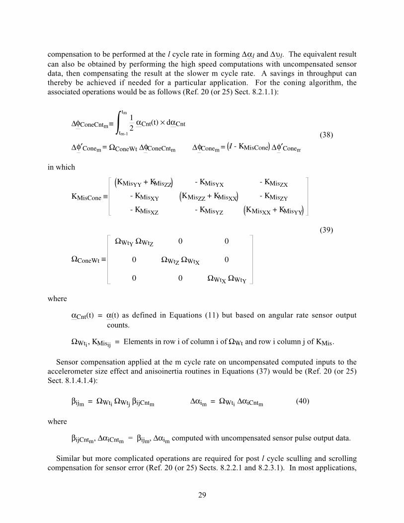
can also be obtained by performing the high speed computations with uncompensated sensordata, then compensating the result at the slower m cycle rate. A savings in throughput canthereby be achieved if needed for a particular application. For the coning algorithm, theassociated operations would be as follows (Ref. 20 (or 25) Sect. 8.2.1.1):

ΔφConeCntm ≡ 12

αCnt(t) × dαCnttm-1

tm

Δφ ′Conem = ΩConeWt ΔφConeCntm ΔφConem = I - KMisCone Δφ ′Conem

(38)

in which

KMisCone ≡

KMisYY + KMisZZ - KMisYX - KMisZX

- KMisXY KMisZZ + KMisXX - KMisZY

- KMisXZ - KMisYZ KMisXX + KMisYY

(39)

ΩConeWt ≡

ΩWtY ΩWtZ 0 0

0 ΩWtZ ΩWtX 0

0 0 ΩWtX ΩWtY

where

αCnt(t) = α(t) as defined in Equations (11) but based on angular rate sensor output

counts.

ΩWti , KMisij = Elements in row i of column i of ΩWt and row i column j of KMis.

Sensor compensation applied at the m cycle rate on uncompensated computed inputs to theaccelerometer size effect and anisoinertia routines in Equations (37) would be (Ref. 20 (or 25)Sect. 8.1.4.1.4):

βijm = ΩWti ΩWtj βijCntm Δαim = ΩWti ΔαiCntm (40)

where

βijCntm, ΔαiCntm = βijm, Δαim computed with uncompensated sensor pulse output data.

Similar but more complicated operations are required for post l cycle sculling and scrollingcompensation for sensor error (Ref. 20 (or 25) Sects. 8.2.2.1 and 8.2.3.1). In most applications,

29

however, ignoring sensor misalignment effects in the sculling, scrolling (and size-effect/anisoinertia) calculations introduces negligible error. Based on this assumption, it then isreasonable to use the direct approach of performing scale factor compensation on the raw angular

rate sensor and accelerometer input data (i.e., applying ΩWt and AWt) at the l cycle rate, and

then applying the scale factor compensated signals as input to the sculling, scrolling (andaccelerometer size effect/anisoinertia) l cycle computation algorithms (Equations (25), (25) and(37)). However, such an approach can still leave significant error in the sculling/scrollingcomputations executed using scale factor compensated sensor data without accelerometer size-effect compensation. Reference 20 (or 25), Section 8.1.4.1 shows that the residual sculling errorcan be accurately approximated and corrected with:

δΔηScul-SizeCm ≈ 12

α(t) × δaSize + δυSizeC(t) × ωIB dttm-1

tm

δυSizeC(t) ≈ δaSize dτtm-1

t(41)

where

δΔηScul-SizeCm = Size effect correction to be applied to a ΔηSculm sculling term

calculated with accelerometer data not containing size effectcompensation.

The δΔηScul-SizeCm correction is applied at the m cycle rate by augmenting the translation

vectors in Equations (12) as follows:

ηm = υm + ΔηSculm - δΔηScul-SizeCm

κm = Sυm + ΔκScrlm - 12

δΔηScul-SizeCm Tm

(42)

Reference 20 (or 25) Section 8.1.4.1.2 shows that δΔηScul-SizeCm in (41) can be accurately

approximated by the following algorithm whose form and magnitude is similar to the basicEquation (37) size-effect compensation algorithm:

δΔηScul-SizeCYm = fSize 12

αZm Δα′Ym + Δα′Ym-1 lZ1 - Δα′Zm + Δα′Zm-1 lY1

- 12

αXm Δα′Xm + Δα′Xm-1 lY3 - Δα′Ym + Δα′Ym-1 lX3

+ βXXm lY3 + βZZm lY1 - βXYm lX3 - βYZm lZ1 (43)

δΔηScul-SizeCZm , δΔηScul-SizeCXm = Similarly by permuting subscripts.

30

where

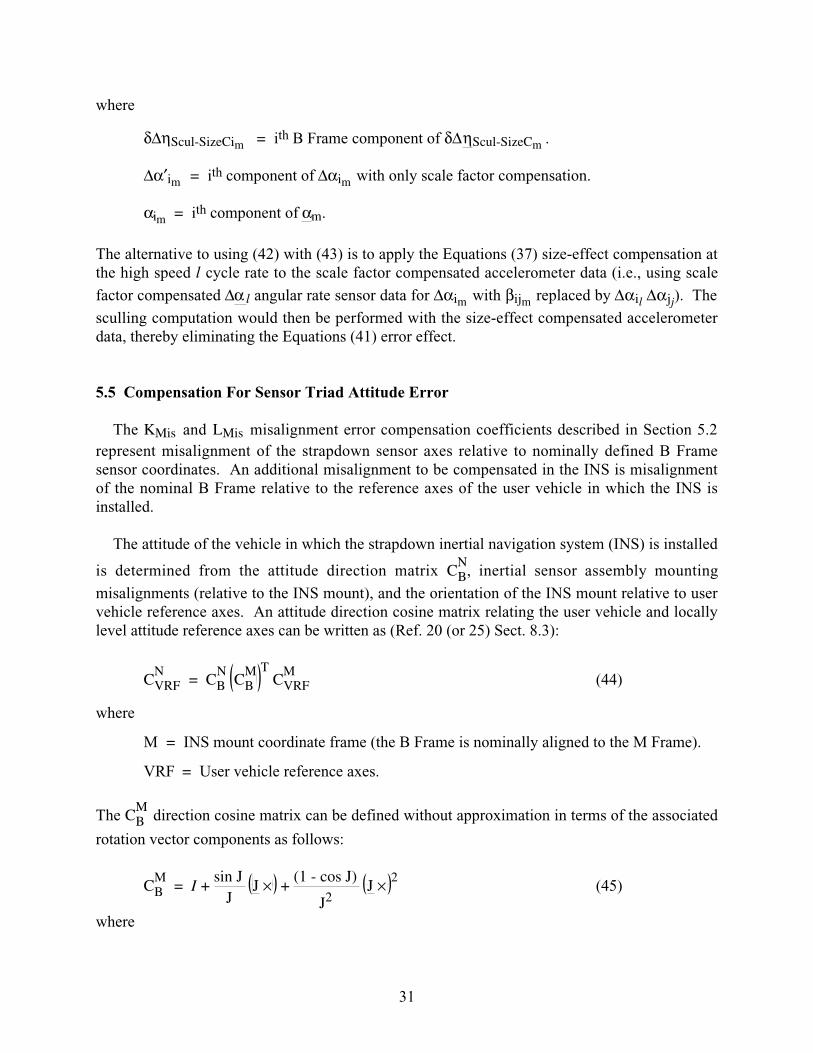
δΔηScul-SizeCim = ith B Frame component of δΔηScul-SizeCm .

Δα′im = ith component of Δαim with only scale factor compensation.

αim = ith component of αm.

The alternative to using (42) with (43) is to apply the Equations (37) size-effect compensation atthe high speed l cycle rate to the scale factor compensated accelerometer data (i.e., using scale

factor compensated Δα l angular rate sensor data for Δαim with βijm replaced by Δαil Δαjj). The

sculling computation would then be performed with the size-effect compensated accelerometerdata, thereby eliminating the Equations (41) error effect.

5.5 Compensation For Sensor Triad Attitude Error

The KMis and LMis misalignment error compensation coefficients described in Section 5.2

represent misalignment of the strapdown sensor axes relative to nominally defined B Framesensor coordinates. An additional misalignment to be compensated in the INS is misalignmentof the nominal B Frame relative to the reference axes of the user vehicle in which the INS isinstalled.

The attitude of the vehicle in which the strapdown inertial navigation system (INS) is installed

is determined from the attitude direction matrix CBN

, inertial sensor assembly mounting

misalignments (relative to the INS mount), and the orientation of the INS mount relative to uservehicle reference axes. An attitude direction cosine matrix relating the user vehicle and locallylevel attitude reference axes can be written as (Ref. 20 (or 25) Sect. 8.3):

CVRFN

= CBN

CBM T

CVRFM

(44)

where

M = INS mount coordinate frame (the B Frame is nominally aligned to the M Frame).

VRF = User vehicle reference axes.

The CBM

direction cosine matrix can be defined without approximation in terms of the associated

rotation vector components as follows:

CBM

= I + sin J

J J × +

(1 - cos J)

J2 J × 2

(45)

where

31

J, J = Sensor triad mount misalignment rotation error vector and its magnitude.

The J components are compensation coefficients measured during system calibration (Ref. 20 (or

25) Sect. 18.4.7.4). The CVRFM

matrix is a function of the particular mount orientation in the user

vehicle.

6. STRAPDOWN INERTIAL NAVIGATION ERRORPROPAGATION EQUATIONS

The overall strapdown INS design process requires supporting analyses to develop and verifyperformance specifications. This generally entails the use of a strapdown INS error model in theform of time rate differential equations that describe the error response of INS computedattitude/velocity/position data. Such error models are also fundamental to the design of Kalmanfilters used, in conjunction with other system inputs, for correcting the INS errors. This sectiondescribes strapdown INS error model equations that represent the INS attitude/velocity/positionnavigation parameter integration routine response to sensor errors (i.e., excluding the effect ofalgorithm and computer finite word-length error, errors that are generally negligible in a welldesigned modern day INS compared to sensor error effects). The term "sensor error" used in thissection refers to the residual error in the sensor signals after applying the Section 5 compensationcorrections. It is only the residual sensor errors that generate INS navigation parameter outputerrors. The residual sensor errors arise from inaccuracy in measuring the sensor compensationcoefficients, sensor random noise outputs that are not accounted for in the compensationalgorithms, short and long term sensor instabilities, and variations in actual sensor performancefrom the analytical models in Section 5.1 that formed the basis for the sensor compensationalgorithms.

6.1 Typical Strapdown Error Parameters

An important part of strapdown INS error model development is the definition (and selection)of attitude/velocity/position error parameters used in the error model and their relationship to theINS integration computed navigation parameters (or to a hypothetical set of INS navigationparameters that are analytically related to the INS computed set). The INS computed navigation

parameters described in Sections 2 - 4 are the CBN

matrix for attitude, the vN vector for velocity,

the CNE

matrix for horizontal earth referenced position, and altitude h for vertical earth referenced

position. These contain 20 individual scalar parameters, each of which develop errors in

response to sensor error. Furthermore, the 18 error parameters associated with the CBN

and CNE

matrices (9 elements each) are not independent due to natural orthogonality/normality constraintsthat govern all direction cosine matrices. To circumvent the problem of dealing with theattendant complexities, navigation error is typically described in terms of three navigation errorvectors (for attitude, velocity, and position), each consisting of three independent error

components. The error in the INS computed navigation parameters (in this case, CBN

, vN, CNE

and

32

h) are analytical functions of the independent error vector parameters. For example, the N Framecomponents of a commonly used set of attitude, velocity, and position error parameters is (Ref.20 or 25 - Sects. 12.2.1-12.2.3 and 12.5) :

ψN× ≡ CEN

I - CBE

CEB

CNE

+ CBN

δαQuantB

×

δVN ≡ CEN

vE

- vE - CBN

δυQuantB

(46)

δRN ≡ CEN

RE

- RE = R CEN

CNE

- I uUpN

+ δh uUpN

where

= Designator for a system computer calculated quantity containing error. The

quantity without the designation is by definition error free (e.g., CBA

is error free

and CBA

contains errors).

ψ = Small angle error rotation vector associated with the computed CBE

attitude matrix.

δV = Error in the computed v velocity vector relative to the earth measured in the E

Frame.

δR = Error in the computed position vector from earth's center R measured in the E

Frame.

δαQuant, δυQuant = Angular rate sensor and accelerometer triad quantization error

residual (remaining after applying quantization compensation -Ref. 20 (or 25) Sect. 8.1.3 and subsections).

The quantization terms in the ψ and δV equations are included to facilitate differential error

equation modeling (See further explanation at conclusion of Section 6.2 to follow).

An equivalent set of attitude, velocity, position error parameters can also be defined that are

more directly related to the CBN

, vN, CNE

, h navigation parameters computed by direct integration

of Equations (1), (6) and (7) (previous references):

γN× ≡ I - CBN

CNB

+ CBN

δαQuantB

×

δvN ≡ vN

- vN - CBN

δυQuantB

(47)

εN× ≡ CEN

CNE

- I

δh ≡ h - h

33

where

γ = Small angle error rotation vector in the computed CBN

attitude matrix.

δv = Error in computed velocity measured in the N Frame.

ε = Small angle error rotation vector in the computed CNE

position matrix.

δh = Error in computed altitude.

The two sets of navigation error parameters are analytically related through (previousreferences):

ψN = γN

- εN

δVN = δvN + εN × vN (48)

δRN = R εN × uUp

N + δh uUp

N

or the equivalent inverse relationships:

εN =

1R

uUpN

× δRN + εZN uUpN

δh = uUpN

⋅ δRN

(49)

δvN = δVN - εN × vN

γN = ψN

+ εN

where

εZN = Local vertical component of ε (projection on the N Frame Z axis along uUp).

R = Distance from earth's center to the current position location (magnitude of R).

6.2 Inertial Sensor Error Parameters

Classical error models for the angular rate sensor and accelerometer triad outputs followingcompensation (in which the error in accelerometer size effect and anisoinertia compensation isignored as negligible) are as follows (Ref. 20 (or 25) Sects. 12.4 - 12.5):

δωIBB

= δKScal/Mis ωIBB

+ δKBias + δ ωRand

δaSFB

= δLScal/Mis aSFB

+ δLBias + δaRand

(50)

34

where

δωIBB

, δaSFB

= Angular rate sensor and accelerometer triad vector error residuals

following sensor compensation but excluding δαQuant, δυQuantquantization compensation error residuals.

δKScal/Mis, δLScal/Mis = Residual angular rate sensor and accelerometer scale-

factor/misalignment error matrices remaining after applying

ΩWt, KMis, AWt, LMis compensation in Equations (34).

δKBias, δLBias = Residual angular rate sensor and accelerometer bias error vectors

remaining after applying KBias, LBias compensation in Equations (34).

Note that the δαQuant, δυQuant quantization compensation error residuals do not appear in the

Equations (50) δωIBB

, δaSFB

error definitions, but instead, show in the Equations (46) - (47)

navigation parameter error vectors. Reference 21 and Reference 20 (or 25) Section 12.5 showthat this form results in the navigation error parameter time rate propagation equations being instandard error state dynamic format (with quantization noise inputs appearing directly, not astheir derivatives) as shown next.

6.3 Error Parameter Propagation Equations

The ψ, δV, δR error parameters defined in Section 6.1 propagate in N Frame coordinates as

(Ref. 20 (or 25) Sects. 12.3.3 and 12.5.1):

ψ. N

= - CBN

δωIB B

- ωINN

× ψ N

+ CBN

ωIB B

× δαQuant

δV.

N = CBN

δaSFB

+ aSFN

× ψN -

gR

δRHN

+ F(h) gR

δR uUpN

- ωIEN

+ ωINN

× δVN + δgMdlN

- aSF N × CB

N δαQuant - CB

N ωIB

B + ωIE

N × CB

N δυQuant

F(h) = 2 For h ≥ 0 F(h) = - 1 For h < 0 (51)

δR.

N = δVN - ωENN

× δRN + CBN

δυQuant

δRHN

= δRN - δR uUpN

δR = uUpN

⋅ δRN

where

35

δRH, δR = Horizontal and upward vertical components of δR.

δgMdl = Modeling error in g produced by variations in true gravity from the model used

in the system computer.

Equations (51) are based on attitude/velocity/position being updated in the strapdown computerat the same algorithm repetition rate. For different repetition rates the quantization terms in theseequations have revised coefficients. Note also that the vertical velocity error equations in (51)are different for positive compared to negative altitudes. This is a manifestation of the differencein gravity model below versus above the earth's surface (Ref. 20 (or 25) Sect. 5.4).

Equations (51) can be integrated to calculate the response of the attitude, velocity, positionerrors in a strapdown INS as impacted by accelerometer, angular rate sensor, and gravity modelapproximation errors. The equations are based on the assumption that the INS navigationparameter integration algorithm error and computer round-off error is negligibly small.

A similar set of N Frame error propagation equations exist for the Equations (47) γ, δv, ε, δh

error parameters (Ref. 20 (or 25) Sects. 12.3.4 and 12.5.2). Equations (51) for ψ, δV, δR and the

equivalent set for γ, δv, ε, δh can be derived from the differential of any set of strapdown inertial

navigation error propagation equations (e.g., the set given in Section 2) with the appropriatedefinitions substituted for the navigation parameter error terms (e.g., Equations (46) or (47)).Alternatively, Reference 20 (or 25) Section 12.3.6 (and subsections) shows that one set of errorparameter propagation equations can be derived from another by applying the equivalencyequations relating the parameters (e.g., Equations (48) or (49)). It is important to recognize thatthe parameters selected to describe the error characteristics of a particular INS can be anyconvenient set and not necessarily those derived from the navigation parameter differentialequations actually implemented in the INS software. Thus, any set of error propagationequations can be used to model the error characteristics of any INS, provided that the errorpropagation equations and INS navigation parameter integration algorithms are analyticallycorrect without singularities over the range of interest, and that the sensor error models areappropriate for the application.

7. CONCLUDING REMARKS

Computational operations in strapdown inertial navigation systems are analytically traceableto basic time rate differential equations of rotational and translational motion as a function ofangular-rate/specific-force-acceleration vectors and local gravitation. Modern day strapdownINS computer capabilities allow the use of navigation parameter integration algorithms based onexact solutions to the differential equations. This considerably simplifies the software validationprocess and can result in a single set of universal algorithms that can be used over a broad rangeof strapdown applications. Exact attitude updating algorithms based on direction cosines or anattitude quaternion are analytically equivalent with identical error characteristics that are afunction of the error in the same computed attitude rotation vector inputs to each. Modern day

36

strapdown computational algorithms and computer capabilities render the computational errornegligible compared to sensor error effects.

The angular-rate/specific-force-acceleration vectors input to the strapdown INS digitalintegration algorithms are measured by angular rate sensors and accelerometers whose errors arecompensated in the strapdown system computer based on classical error models for the inertialsensors. Strapdown INS attitude/velocity/position output errors are produced by errorsremaining in the inertial sensor signals following compensation (due to sensor error modelinaccuracies, sensor error instabilities, sensor calibration errors) and to gravity modeling errors.Resulting INS navigation error characteristics can be defined by various attitude, velocity,position error parameters that are analytically equivalent. Any set of navigation parameter errorpropagation equations can be used to predict the error performance of any strapdown INS. Thenavigation error parameters used in the error propagation equations do not have to be directlyrelated to the navigation parameters used in the strapdown INS computer integration algorithms.

REFERENCES

1. Bortz J. E., “A New Mathematical Formulation for Strapdown Inertial Navigation”, IEEETransactions on Aerospace and Electronic Systems, Volume AES-7, No. 1, January1971, pp. 61-66.

2. Britting, K. R., Inertial Navigation System Analysis, John Wiley and Sons, New York, 1971.

3. “Department Of Defense World Geodetic System 1984”, NIMA TR8350.2, Third Edition, 4July 1997.

4. Goodman, L.E. and Robinson, A.R., "Effects of Finite Rotations on Gyroscope SensingDevices", Journal of Applied Mechanics, Vol. 25, June 1958.

5. Ignagni, M. B., “Optimal Strapdown Attitude Integration Algorithms”, AIAA Journal OfGuidance, Control, And Dynamics, Vol. 13, No. 2, March-April 1990, pp. 363-369.

6. Ignagni, M. B., “Efficient Class Of Optimized Coning Compensation Algorithms”, AIAAJournal Of Guidance, Control, And Dynamics, Vol. 19, No. 2, March-April 1996, pp.424-429.

7. Ignagni, M. B., “Duality of Optimal Strapdown Sculling and Coning CompensationAlgorithms”, Journal of the ION, Vol. 45, No. 2, Summer 1998.

8. Jordan, J. W., “An Accurate Strapdown Direction Cosine Algorithm”, NASA TN-D-5384,September 1969.

9. Kachickas, G. A., “Error Analysis For Cruise Systems”, Inertial Guidance, edited by Pitman,G. R., Jr., John Wiley & Sons, New York, London, 1962.

37

10. Laning, J.H., Jr., "The Vector Analysis of Finite Rotations and Angles", MassachusettsInstitute of Technology, Cambridge, Instrumentation Laboratory Special Report 6398-S-3, 1949.

11. Litmanovich, Y. A., Lesyuchevsky, V. M. & Gusinsky, V. Z., “Two New Classes ofStrapdown Navigation Algorithms”, AIAA Journal Of Guidance, Control, And Dynamics,Vol. 23, No. 1, January- February 2000.

12. Mark, J.G. & Tazartes, D.A., “On Sculling Algorithms”, 3rd St. Petersburg InternationalConference On Integrated Navigation Systems, St. Petersburg, Russia, May 1996.

13. Miller, R., “A New Strapdown Attitude Algorithm”, AIAA Journal Of Guidance, Control,And Dynamics, Vol. 6, No. 4, July-August 1983, pp. 287-291.

14. Roscoe, K. M., “Equivalency Between Strapdown Inertial Navigation Coning and ScullingIntegrals/Algorithms”, AIAA Journal Of Guidance, Control, And Dynamics, Vol. 24, No.2, March-April 2001, pp. 201-205.

15. Savage, P. G., “A New Second-Order Solution for Strapped-Down Attitude Computation”,AIAA/JACC Guidance & Control Conference, Seattle, Washington, August 15-17, 1966.

16. Savage, P. G., “Strapdown Sensors”, Strapdown Inertial Systems - Theory And Applications,NATO AGARD Lecture Series No. 95, June 1978, Section 2.

17. Savage, P. G., “Strapdown System Algorithms”, Advances In Strapdown Inertial Systems,NATO AGARD Lecture Series No. 133, May 1984, Section 3.

18. Savage, P. G., “Strapdown Inertial Navigation System Integration Algorithm Design Part 1 -Attitude Algorithms”, AIAA Journal Of Guidance, Control, And Dynamics, Vol. 21, No.1, January-February 1998, pp. 19-28.

19. Savage, P. G., “Strapdown Inertial Navigation System Integration Algorithm Design Part 2 -Velocity and Position Algorithms”, AIAA Journal Of Guidance, Control, And Dynamics,Vol. 21, No. 2, March-April 1998, pp. 208-221.

20. Savage, P. G., Strapdown Analytics, First Edition, Strapdown Associates, Inc., Maple Plain,Minnesota, 2000.

21. Savage, P. G., "Analytical Modeling of Sensor Quantization in Strapdown Inertial NavigationError Equations", AIAA Journal Of Guidance, Control, And Dynamics, Vol. 25, No. 5,September-October 2002, pp. 833-842.

22. Savage, P. G., "Strapdown System Computational Elements", Advances In NavigationSensors and Integration Technology, NATO RTO Lecture Series No. 232, October 2003,Section 3.

38

23. Savage, P. G., "A Unified Mathematical Framework For Strapdown Algorithm Design",AIAA Journal Of Guidance, Control, And Dynamics, Vol. 29, No. 2, March-April 2006,pp. 237-249.

24. Savage, P. G., "Reply by the Author to Y. Wu", AIAA Journal Of Guidance, Control, AndDynamics, Vol. 29, No. 6, November-December 2006, pp. 1485-1486.

25. Savage, P. G., Strapdown Analytics - Second Edition, Strapdown Associates, Inc., MaplePlain, Minnesota, 2007.

26. Savage, P. G., "Performance Analysis Of Strapdown Systems", Low Cost Navigation Sensorsand Integration Technology, NATO RTO-EN-SET-116(2008), Section 10, published in2009, also reformatted for Web Free Access as SAI-WBN-14011, June 2, 2015 atwwww.strapdownassociates.com.

27. Wu, Y. "Comment on 'A Unified Mathermatical Framework for Strapdown AlgorithmDesign' ", AIAA Journal Of Guidance, Control, And Dynamics, Vol. 29, No. 6,November-December 2006, pp. 1482-1484.

39