NASA/CR-97-206268

ICASE Report No. 97-68

_th,NNIVERSARY

Essential Elements of Computational Algorithms

for Aerodynamic Analysis and Design

Antony Jameson

December 1997

The NASA STI Program Off'we... in Profile

Since its founding, NASA has been dedicated

to the advancement of aeronautics and space

science. The NASA Scientific and Technical

Information (STI) Program Office plays a key

part in helping NASA maintain this

important role.

The NASA STI Program Office is operated by

Langley Research Center, the lead center forNASA's scientific and technical information.

The NASA STI Program Office provides

access to the NASA STI Database, the

largest collection of aeronautical and space

science STI in the world. The Program Officeis also NASA's institutional mechanism for

disseminating the results of its research and

development activities. These results are

published by NASA in the NASA STI Report

Series, which includes the following report

types:

TECHNICAL PUBLICATION. Reports of

completed research or a major significant

phase of research that present the results

of NASA programs and include extensive

data or theoretical analysis. Includes

compilations of significant scientific andtechnical data and information deemed

to be of continuing reference value. NASA

counter-part or peer-reviewed formal

professional papers, but having less

stringent limitations on manuscript

length and extent of graphic

presentations.

TECHNICAL MEMORANDUM.

Scientific and technical findings that are

preliminary or of specialized interest,

e.g., quick release reports, working

papers, and bibliographies that containminimal annotation. Does not contain

extensive analysis.

CONTRACTOR REPORT. Scientific and

technical findings by NASA-sponsored

contractors and grantees.

CONFERENCE PUBLICATIONS.

Collected papers from scientific and

technical conferences, symposia,

seminars, or other meetings sponsored or

co-sponsored by NASA.

SPECIAL PUBLICATION. Scientific,

technical, or historical information from

NASA programs, projects, and missions,

often concerned with subjects having

substantial public interest.

TECHNICAL TRANSLATION. English-

language translations of foreign scientific

and technical material pertinent toNASA's mission.

Specialized services that help round out the

STI Program Office's diverse offerings include

creating custom thesauri, building customized

databases, organizing and publishing

research results.., even providing videos.

For more information about the NASA STI

Program Office, you can:

Access the NASA STI Program Home

Page at http:/Iwww.sti.nasa.govlSTI-

homepage.html

• Email your question via the Internet to

help @ sti.nasa.gov

• Fax your question to the NASA Access

Help Desk at (301) 621-0134

• Phone the NASA Access Help Desk at

(301) 621-0390

Write to:

NASA Access Help Desk

NASA Center for AeroSpace Information

800 Elkridge Landing Road

Linthicum Heights, MD 21090-2934

NASA/CR-97-206268

ICASE Report No. 97-68

Essential Elements of Computational Algorithms

for Aerodynamic Analysis and Design

Antony Jameson

Stanford University

Institute for Computer Applications in Science and Engineering

NASA Langley Research Center

Hampton, VA

Operated by Universities Space Research Association

National Aeronautics and

Space Administration

Langley Research Center

Hampton, Virginia 23681-2199

Prepared for Langley Research Centerunder Contracts NAS 1-97046 & NAS 1-19480

December 1997

Available from the following:

N_A_SA_Center for AeroSpace Information (CASI)

800 Elkridge Landing Road

Linthicum Heights, ME) 21090-2934

(301) 621-0390

.N_ati0nal- Technical Information Se_ (NTIS)

5285 Port Royal Road .....

Springfield, VA 22161-2171

(703) 487-4650

ESSENTIAL ELEMENTS OF COMPUTATIONAL ALGORITHMS FOR AERODYNAMIC

ANALYSIS AND DESIGN*

ANTONY JAMESON t

Abstract. This paper traces the development of computational fluid dynamics as a tool for aircraft

design. It addresses the requirements for effective industrial use, and trade-offs between modeling accuracy

and computational costs. Essential elements of algorithm design are discussed in detail, together with a

unified approach to the design of shock capturing schemes. Finally, the paper discusses the use of techniques

drawn from control theory to determine optimal aerodynamic shapes. In the future multidisciplinary analysis

and optimization should be combined to provide an integrated design environment.

Key words, computational fluid dynamics, aerodynamic design, optimization

Subject classification. Fluid Mechanics

1. Introduction. Computational methods first began to have a significant impact on aerodynamics

analysis and design in the period of 1965-75. This decade saw the introduction of panel methods which

could solve the linear flow models for arbitrarily complex geometry in both subsonic and supersonic flow

[68, 164,200]. It also saw the appearance of the first satisfactory methods for treating the nonlinear equations

of transonic flow [135, 134, 75, 76, 51, 63], and the development of the hodograph method for the design of

shock free supercritical airfoils [19].

Computational Fluid Dynamics (CFD) has now matured to the point at which it is widely accepted as a

key tool for aerodynamic design. Algorithms have been the subject of intensive development for the past two

decades. The principles underlying the design and implementation of robust schemes which can accurately

resolve shock waves and contact discontinuities in compressible flows are now quite well established. It is

also quite well understood how to design high order schemes for viscous flow, including compact schemes

and spectral methods. Adaptive refinement of the mesh interval (h) and the order of approximations (p)

has been successfully exploited both separately and in combination in the h-p method [138]. A continuing

obstacle to the treatment of configurations with complex geometry has been the problem of mesh generation.

Several general techniques have been developed, including algebraic transformations and methods based on

the solution of elliptic and hyperbolic equations. In the last few years methods using unstructured meshes

have also begun to gain more general acceptance. The Dassault-INRIA group led the way in developing a

finite element method for transonic potential flow. They obtained a solution for a complete Falcon 50 as

early as 1982 [29]. Euler methods for unstructured meshes have been the subject of intensive development

by several groups since 1985 [118, 90, 89, 183, 18], and Navier-Stokes methods on unstructured meshes have

also been demonstrated [126, 127, 17].

Despite the advances that have been made, CFD is still not being exploited as effectively as one would

like in the design process. This is partly due to the long set-up and high costs, both human and computational

of complex flow simulations. The essential requirements for industrial use are"

1. assured accuracy

*This paper is the result of the Theodorsen Lecture, which was supported by the Institute for Computer Applications in

Science and Engineering (ICASE) and the National Aeronautics and Space Administration (NASA) under NASA Contract Nos.NAS1-19480 and NAS1-97046.

tDepartment of Aeronautics and Astronautics, Stanford University, Durand Building, Stanford, CA 94305-4035

2. acceptablecomputationalandhumancosts3. fastturnaround.

Improvementsarestill neededin all threeareas.In particular,thefidelityof modellingof highReynoldsnumberviscousflowscontinuesto be limitedby computationalcosts. Consequently accurate and cost

effective simulation of viscous flow at Reynolds numbers associated with full scale flight, such as the prediction

of high lift devices, remains a challenge. Several routes are available toward the reduction of computational

costs, including the reduction of mesh requirements by the use of higher order schemes, improved convergence

to a steady state by sophisticated acceleration methods, fast inversion methods for implicit schemes, and the

exploitation of massively parallel computers.

Another factor limiting the effective use of CFD is the lack of good interfaces to computer aided design

(CAD) systems. The geometry models provided by existing CAD systems often fail to meet the requirements

of continuity and smoothness needed for flow simulation, with the consequence that they must be modified

before they can be used to provide the input for mesh generation. This bottleneck, which impedes the

automation of the mesh generation process, needs to be eliminated, and the CFD software should be fully

integrated in a numerical design environment. In addition to more accurate and cost-effective flow prediction

methods, better optimizations methods are also needed, so that not only can designs be rapidly evaluated,

but directions of improvement can be identified. Possession of techniques which result in a faster design

cycle gives a crucial advantage in a competitive environment.

A critical issue, examined in the next section, is the choice of mathematical models. What level of

complexity is needed to provide sufficient accuracy for aerodynamic design, and what is the impact on cost

and turn-around time? Section 3 addresses the design of numerical algorithms for flow simulation. Sectlon

4 presents the results of some numerical calculations which require moderate computer resources and could

be completed with the fast turn-around required by industrial users. Section 5 discusses automatic design

procedures which can be used to produce optimum aerodynamic designs. Finally, Section 6 offers an outlook

for the future.

2. The Complexity of Fluid Flow and Mathematical Modeling.

2.1. The Hierarchy of Mathematical Models. Many critical phenomena of fluid flow, such as shock

waves and turbulence, are essentially non-linear. They also exhibit extreme disparities of scales. While the

actual thickness of a shock wave is of the order of a mean free path of the gas particles, on a macroscopic

scale its thickness is essentially zero. In turbulent flow energy is transferred from large scale motions to

progressively smaller eddies until the scale becomes so small that the motion is dissipated by viscosity. The

ratio of the length scale of the global flow to that of the smallest persisting eddies is of the order Re¼, where

Re is the Reynolds number, typically in the range of 30 million for an aircraft. In order to resolve such scales

in all three space directions a computational grid with the order of Re_ cells would be required. This is

beyond the range of any current or foreseeable computer. Consequently mathematical models with varying

degrees of simplification have to be introduced in order to make computational simulation of flow feasible

and produce viable and cost-effective methods.

Figure 1 (supplied by Pradeep Raj) indicates a hierarchy of models at different levels of simplification

which have proved useful in practice. Efficient flight is generally achieved by the use of smooth and stream-

lined shapes which avoid flow separation and minimize viscous effects, with the consequence that useful

predictions can be made using inviscid models. Invisc|d Calculations with boundary layer corrections can

provide quite accurate predictions of lift and drag when the flow remains attached, but iteration between the

inviscid outer solution and the inner boundary layer solution becomes increasingly difficult with the onset

ofseparation.Proceduresforsolvingthefull viscousequationsarelikelyto beneededforthesimulationofarbitrarycomplexseparatedflows,whichmayoccurat highanglesofattackor withbluffbodies.In orderto treatflowsat highReynoldsnumbers,oneisgenerallyforcedto estimateturbulenteffectsby Reynoldsaveragingof the fluctuatingcomponents.Thisrequirestheintroductionof a turbulencemodel.As theavailablecomputingpowerincreasesonemayalsoaspireto largeeddysimulation(LES)in whichthelargerscaleeddiesaredirectlycalculated,whiletheinfluenceofturbulenceatscalessmallerthanthemeshintervalisrepresentedbya subgridscalemodel.

Ill. Euler (1980:) I

+ Rotation

Nonlinear Potential (1970s)

/7// / I

FIG. 1. Hierarchy of Fluid Flow Models

2.2. Computational Costs. Computational costs vary drastically with the choice of mathematical

model. Panel methods can be effectively used to solve the linear potential flow equation with higher-end

personal computers (with an Intel Pentium microprocessor, for example). Studies of the dependency of the

result on mesh refinement, performed by this author and others, have demonstrated that inviscid transonic

potential flow or Euler solutions for an airfoil can be accurately calculated on a mesh with 160 cells around

the section, and 32 cells normal to the section. Using multigrid techniques 10 to 25 cycles are enough to

obtain a converged result. Consequently airfoil calculations can be performed in seconds on a Cray YMP, and

can also be performed on Pentium-class personal computers. Correspondingly accurate three-dimensional

inviscid calculations can be performed for a wing on a mesh, say with 192×32×48 -- 294,912 cells, in about

5 minutes on a single processor Cray YMP, or less than a minute with eight processors, or in less than an

hour on a workstation such as a Silicon Graphics Indigo 2.

Viscous simulations at high Reynolds numbers require vastly greater resources. Careful two-dimensional

studies of mesh requirements have been carried out at Princeton by Martinelli [122]. He found that on the

order of 32 mesh intervals were needed to resolve a turbulent boundary layer, in addition to 32 intervals be-

tween the boundary layer and the far field, leading to a total of 64 intervals. In order to prevent degradations

in accuracy and convergence due to excessively large aspect ratios (in excess of 1,000) in the surface mesh

cells, the chordwise resolution must also be increased to 512 intervals. Reasonably accurate solutions can be

obtained in a 512×64 mesh in 100 multigrid cycles. Translated to three dimensions, this would imply the

need for meshes with 5-10 million cells (for example, 512×64x256 -- 8,388,608 cells as shown in Figure 2).

When simulations are performed on less fine meshes with, say, 500,000 to 1 million cells, it is very hard to

avoid mesh dependency in the solutions as well as sensitivity to the turbulence model.

A typical algorithm requires of the order of 5,000 floating point operations per mesh point in one

multigrid iteration. With 10 million mesh points, the operation count is of the order of 0.5x 1011 per cycle.

Given a computer capable of sustaining 1011 operations per second (100 gigaflops), 200 cycles could then be

performed in 100 seconds. Simulations of unsteady viscous flows (flutter, buffet) would be likely to require

\\

S12 oe_ _ the 'w_ 8 to limit

the nlesh aspect ,taliO (to about 1000)

/ i1?

Total: _I2x64x258= 8 389 608 ccAls

FIG. 2. Mesh Requirement_ for a Viscous Simulation

1,000 10,000 time steps. A further progression to large eddy simulation of complex configurations would

require even greater resources. The following estimate is due to W.H. Jou [98]. Suppose that a conservative

estimate of the size of eddies in a boundary layer that ought to be resolved is 1/5 of the boundary layer

thickness. Assuming that 10 points are needed to resolve a single eddy, the mesh interval should then be 1/50

of the boundary layer thickness. Moreover, since the eddies are three-dimensional, the same mesh interval

should be used in all three directions. Now, if the boundary layer thickness is of the order of 0.01 of the

chord length, 5,000 intervals will be needed in the chordwise direction, and for a wing with an aspect ratio

of 10, 50,000 intervals will be needed in the spanwise direction. Thus, of the order of 50 x 5,000 x 50,000

or 12.5 billion mesh points would be needed in the boundary layer. If the time dependent behavior of the

eddies is to be fully resolved using time steps on the order of the time for a wave to pass through a mesh

interval, and one allows for a total time equal to the time required for waves to travel three times the length

of the chord, of the order of 15,000 time steps would be needed. A more refined estimate which allows for

the varying ttaickness of the boundary layer, recently made by Spalart et al. [179], suggests an even more

severe requirement. Performance beyond the teraflop (1012 operations per second) will be needed to attempt

calculations of this nature, which also have an information content far beyond what is needed for enginering

analysis and design. The designer does not need to know the details of the eddies in the boundary layer.

The primary purpose of such calculations is to improve the calculation of averaged quantities such as skin

friction, and the prediction of global behavior such as the onset of separation. The main current use of

Navier-Stokes and large eddy simulations is to try to gain an improved insight into the physics of turbulent

flow, which may in turn lead to the development of more comprehensive and reliable turbulence models.

2.3. Turbulence Modeling. It is doubtful whether a universally valid turbulence model, capable of

describing all complex flows, could be devised [61]. Algebraic models [35, 14] have proved fairly satisfactory

for the calculation of attached and slightly separated wing flows. These models rely on the boundary layer

concept, usually incorporating separate formulas for the inner and outer layers, and they require an estimate

ofa lengthscalewhichdependsonthethicknessof the boundary layer. The estimation of this quantity by

a search for a maximum of the vorticity times a distance to the wall, as in the Baldwin-Lomax model, can

lead to ambiguities in internal flows, and also in complex vortical flows over slender bodies and highly swept

or delta wings [47, 123]. The Johnson-King model [96], which allows for non-equilibrium effects through the

introduction of an ordinary differential equation for the maximum shear stress, has improved the prediction

of flows with shock induced separation [165, 99].

Closure models depending on the solution of transport equations are widely accepted for industrial

applications. These models eliminate the need to estimate a length scale by detecting the edge of the

boundary layer. Eddy viscosity models typically use two equations for the turbulent kinetic energy k and

the dissipation rate e, or a pair of equivalent quantities [97, 199, 180, 1, 131, 40]. Models of this type generally

tend to present difficulties in the region very close to the wall. They also tend to be badly conditioned for

numerical solution. The k - l model [173] is designed to alleviate this problem by taking advantage of the

linear behaviour of the length scale I near the wall. In an alternative approach to the design of models which

are more amenable to numerical solution, new models requiring the solution of one transport equation have

recently been introduced [13, 178]. The performance of the algebraic models remains competitive for wing

flows, but the one- and two-equation models show promise for broader classes of flows. In order to achieve

greater universality, research is also being pursued on more complex Reynolds stress transport models, which

require the solution of a larger number of transport equations.

Another direction of research is the attempt to devise more rational models via renormalization group

(RNG) theory [203, 174]. Both algebraic and two-equation k - e models devised by this approach have shown

promising results [124].

The selection of sufficiently accurate mathematical models and a judgment of their cost effectiveness

ultimately rests with industry. Aircraft and spacecraft designs normally pass through the three phases of

conceptual design, preliminary design, and detailed design. Correspondingly, the appropriate CFD models

will vary in complexity. In the conceptual and preliminary design phases, the emphasis will be on relatively

simple models which can give results with very rapid turn-around and low computer costs, in order to evaluate

alternative configurations and perform quick parametric studies. The detailed design stage requires the most

complete simulation that can be achieved with acceptable cost. In the past, the low level of confidence that

could be placed on numerical predictions has forced the extensive use of wind tunnel testing at an early stage

of the design. This practice was very expensive. The limited number of models that could be fabricated also

limited the range of design variations that could be evaluated. It can be anticipated that in the future, the

role of wind tunnel testing in the design process will be more one of verification. Experimental research to

improve our understanding of the physics of complex flows will continue, however, to play a vital role.

3. CFD Algorithms.

3.1. Difficulties of Flow Simulation. The computational simulation of fluid flow presents a number

of severe challenges for algorithm design. At the level of inviscid modeling, the inherent nonlinearity of the

fluid flow equations leads to the formation of singularities such as shock waves and contact discontinuities.

Moreover, the geometric configurations of interest are extremely complex, and generally contain sharp edges

which lead to the shedding of vortex sheets. Extreme gradients near stagnation points or wing tips may also

lead to numerical errors that can have global influence. Numerically generated entropy may be convected

from the leading edge for example, causing the formation of a numerically induced boundary layer which

can lead to separation. The need to treat exterior domains of infinite extent is also a source of difficulty.

Boundary conditions imposed at artificial outer boundaries may cause reflected waves which significantly

interferewith theflow.Whenviscouseffectsarealsoincludedin thesimulation,theextremedifferenceofthc scalesin theviscousboundarylayerandtheouterflow,whichis essentiallyinviscid,isanothersourceofdifficulty,forcingtheuseofmesheswithextremevariationsin meshinterval.ForthesereasonsCFD, has

been a driving force for the development of numerical algorithms.

3.2. Structured and Unstructured Meshes. The algorithm designer faces a number of critical deci-

sions. The first choice that must be made is the nature of the mesh used to divide the flow field into discrete

subdomains. The discretization procedure must allow for the treatment of complex configurations. The

principal alternatives are Cartesian meshes, body-fitted curvilinear meshes, and unstructured tetrahedral

meshes. Each of these approaches has advantages which have led to their use. The Cartesian mesh mini-

mizes the complexity of the algorithm at interior points and facilitates the use of high order discretization

procedures, at the expense of greater complexity, and possibly a loss of accuracy, in the treatment of bound-

ary conditions at curved surfaces. This difficulty may be alleviated by using mesh refinement procedures

near the surface. With their aid, schemes which use Cartesian meshes have recently been developed to treat

very complex configurations [130, 166, 26, 103].

Body-fitted meshes have been widely used and are particularly well suited to the treatment of viscous

flow because they readily allow the mesh to be compressed near the body surface. With this approach, the

problem of mesh generation itself has proved to be a major pacing item. The most commonly used procedures

are algebraic transformations [11, 52, 55, 175], methods based on the solution of elliptic equations, pioneered

by Thompson [189, 190, 176, 177], and methods based on the solution of hyperbolic equations marching out

from the body [181]. In order to treat very complex configurations it generally proves expedient to use a

multiblock [198, 167] procedure, with separately generated meshes in each block, which may then be patched

at block faces, or allowed to overlap, as in the Chimera scheme [23, 24]. While a number of interactive

software systems for grid generation have been developed, such as EAGLE, GRIDGEN, and ICEM, the

generation of a satisfactory grid for a very complex configuration may require months of effort.

The alternative is to use an unstructured mesh in which the domain is subdivided into tetrahedra.

This in turn requires the development of solution algorithms capable of yielding the required accuracy on

unstructured meshes. This approach has been gaining acceptance, as it is becoming apparent that it can lead

to a speed-up and reduction in the cost of mesh generation that more than offsets the increased complexity

and cost of the flow simulations. Two competing procedures for generating triangulations which have both

proved successful are Delaunay triangulation [48, 17], based on concepts introduced at the beginning of the

century by Voronoi [196], and the moving front method [119].

3.3. Finite Difference, Finite Volume, and Finite Element Schemes. Associated with choice

of mesh type is the formulation of the discretization procedure for the equations of fluid flow, which can be

expressed as differential conservation laws. In the Cartesian tensor notation, let xi be the coordinates, p, p,

TI and E the pressure, density, temperature, and total energy, and ui the velocity components. Using the

convention that summation over j -- 1, 2, 3 is implied by a repeated subscript j, each conservation equation

has the form

Ow Ofj Ofv_

(1) 0-7 + Oxj Oxj = O.

where ]_ are the inviscid (convective) fluxes, and fv3 arc the viscous fluxes. For the mass equation

w = p, f¢ = pu s .

Forthei momentum equation

wi = pui, fij = puiuj + pSij, fv,_ = crij,

where aij is the viscous stress tensor. For the energy equation

k °T 'w= pE, fj ----pHuj, fv_ =ajkuk-- OXj

where k is the coefficient of thermal conductivity. The pressure is related to the density and energy by the

equation of state

in which 7 is the ratio of specific heats and the stagnation enthalpy is given by

H=E+ pP

while

1E = c_T + _uiui

where cv is the specific heat at constant volume. In the Navier-Stokes equations the viscous stresses are

assumed to be linearly proportional to the rate of strain, or

(3) a_¢=_ \ Oxj + Ox, ] + _j \ Ozk ] '

where # and A are the coefficients of viscosity and bulk viscosity, and usually A = -2/_/3. The coefficient of

thermal conductivity and temperature are given by the relations

k_%/_ T= P__Pr ' Rp

where ap is the specific heat at constant pressure, R is the gas constant, and Pr is the Prandtl number.

The finite difference method, which requires the use of a Cartesian or a structured curvilinear mesh,

directly approximates the differential operators appearing in these equations. In the finite volume method

[120], the discretization is accomplished by dividing the domain of the flow into a large number of small

subdomains, and applying the conservation laws in the integral form

Here F is the flux appearing in equation (1) and dS is the directed surface element of the boundary 0fl of

the domain ft. The use of the integral form has the advantage that no assumption of the differentiability

of the solutions is implied, with the result that it remains a valid statement for a subdomain containing a

shock wave. In general the subdomains could be arbitrary, but it is convenient to use either hexahedral cells

in a body conforming curvilinear mesh or tetrahedrons in an unstructured mesh.

Alternative discretization schemes may be obtained by storing flow variables at either the cell centers or

the vertices. These variations are illustrated in Figure 3 for the two-dimensional case. With a cell-centered

scheme the discrete conservation law takes the form

p

Figure 3a: Cell Centered Scheme.

Figure 3b: Vertex Scheme.

Fro. 3. Structured and Un_str_ctured Discretization_.

d(4) wv + F_, f.s = 0,

faces

where V is the cell volume, and f is now a numerical estimate of the flux vector through each face. f may

be evaluated from values of the flow variables in the cells separated by each face, using upwind biasing to

allow for the directions of wave propagation. With hexahedral cells, equation (4) is very similar to a finite

difference scheme in curvilinear coordinates. Under a transformation to curvilinear coordinates _j, equation

(1) becomcs

(5) 0---t _ J =0,

[o__x1where J is the 3acobian determinant of the transformation matrix [a_, !" The transformed flux J_fj

corresponds to the dot product of the flux f with a vector face area J_, while J represents the transfor-

mation of the cell volume. The finite volume form (4) has the advantages that it is valid for both structured

and unstructured meshes, and that it assures that a uniform flow exactly satisfies the equations, because

Y]faces S -- 0 for a closed control volume. Finite difference schemes do not necessarily satisfy this constraint

because of the discretization errors in evaluating _ and the inversion of the transformation matrix. AOx_

cell-vertex finite volume scheme can be derived by taking the union of the cells surrounding a given vertex

as the control volume for that vertex [64, 81, 156]. In equation (4), V is now the sum of the volumes of the

surrounding cells, while the flux balance is evaluated over the outer faces of the polyhedral control volume.

In the absence of upwind biasing the flux vector is evaluated by averaging over the corners of each face. This

has the advantage of remaining accurate on an irregular or unstructured mesh. An alternative route to the

discrete equations is provided by the finite element method. Whereas the finite difference and finite volume

methods approximate the differential and integral operators, the finite element method proceeds by inserting

an approximate-solution into the exact equations. On multiplying by a test function ¢ and integrating by

parts over space, one obtains the weak form

0(6) -_ f f fnewdl2= f /fnf.Vedf_- f _onef.dS

which is also valid in the presence of discontinuities in the flow. In the Galerkin method the approximate

solution is expanded in terms of the same family of functions as those from which the test functions are

drawn. By choosing test functions with local support, separate equations are obtained for each node. For

example, if a tetrahedral mesh is used, and ¢ is piecewise linear, with a nonzero value only at a single node,

the equations at each node have a stencil which contains only the nearest neighbors. In this case the finite

element approximation corresponds closely to a finite volume scheme. If a piecewise linear approximation

to the flux f is used in the evaluation of the integrals on the right hand side of equation (6), these integrals

reduce to formulas which are identical to the flux balance of the finite volume scheme.

Thus the finite difference and finite volume methods lead to essentially similar schemes on structured

meshes, while the finite volume method is essentially equivalent to a finite element method with linear

elements when a tetrahedral mesh is used. Provided that the flow equations are expressed in the conservation

law form (1), all three methods lead to an exact cancellation of the fluxes through interior cell boundaries, so

that the conservative property of the equations is preserved. The important role of this property in ensuring

correct shock jump conditions was pointed out by Lax and Wendroff [105].

3.4. Non-oscillatory Shock Capturing Schemes.

3.4.1. Local Extremum Diminishing (LED) Schemes. The discretization procedures which have

been described in the last section lead to nondissipative approximations to the Euler equations. Dissipative

terms may be needed for two reasons. The first is the possibility of undamped oscillatory modes. The second

reason is the need for the clean capture of shock waves and contact discontinuities without undesirable

oscillations. An extreme overshoot could result in a negative value of an inherently positive quantity such as

the pressure or density. The next sections summarize a unified approach to the construction of nonoscillatory

schemes via the introduction of controlled diffusive and antidiffusive terms. This is the line adhered to in

the author's own work.

The development of non-oscillatory schemes has been a prime focus of algorithm research for compressible

flow. Consider a general semi-discrete scheme of the form

d=(7) -

k#j

A maximum cannot increase and a minimum cannot decrease if the coefficients cjk are non-negative, since

at a maximum Vk -- vj < 0, and at a minimum vk - vj >__0. Thus the condition

(8) cjk >0, k # j

is sufficient to ensure stability in the maximum norm. Moreover, if the scheme has a compact stencil, so that

cjk = 0 when j and k are not nearest neighbors, a local maximum cannot increase and local minimum cannot

decrease. This local extremum diminishing (LED) property prevents the birth and growth of oscillations.

The one-dimensional conservation law

Ou Of u()=0

provides a useful model for analysis. In this case waves are propagated with a speed a(u) = -_, and the

solution is constant along the characteristics -_ = a(u). Thus the LED property is satisfied. In fact the

totalvariation

/?TV(u) = dxO0

of a solution of this equation does not increase, provided that any discontinuity appearing in the solution

satisfies an entropy condition [104]. Harten proposed that difference schemes ought to be designed so that the

discrete total variation cannot increase [65]. If the end values are fixed, the total variation can be expressed

as

=2 (_ maxima -- _ minima ).TV(u)

Thus a LED scheme is also total variation diminishing (TVD). Positivity conditions of the type expressed in

equations (7) and (8) lead to diagonally dominant schemes, and are the key to the elimination of improper

oscillations. The positivity conditions may be realized by the introduction of diffusive terms or by the use of

upwind biasing in the discrete scheme. Unfortunately, they may also lead to severe restrictions on accuracy

unless the coefficients have a complex nonlinear dependence on the solution.

3.4.2. Artificial Diffusion and Upwinding. Following the pioneering work of Godunov [60], a variety

of dissipative and upwind schemes designed to have good shock capturing properties have been developed

during the past two decades [182, 27, 107, 108, 163, 142, 65, 141, 185, 8, 79, 204, 73, 201, 16, 15, 17]. If the

one-dimensional scalar conservation law

(9)

is represented by a three point scheme

Ov O j, v( )=0

dvj _

d-t - c_+½ (vj+l - vj) + cj_½ (vj-1 - vs),

the scheme is LED if

(10) c++½ >__O, cs_½ > O.

A conservative semidiscrete approximation to the one-dimensional conservation law can be derived by sub-

dividing the line into cells. Then the evolution of the value vj in the jth cell is given by

(11) Ax_tJ + hi+½ - hi_½ = O,

where hi+ ½ is an estimate of the flux between cells j and j + 1. The simplest estimate is the arithmetic

average (fj+l + fj)/2, but this leads to a scheme that does not satisfy the positivity conditions. To correct

this, one may add a dissipative term and set

1(12) hi+½ _- _ (fj+i -t- fj) -- O_j+½ (Vj+ 1 -- Vj).

In order to estimate the required value of the coefficient c_j+½, let aj+½ be a numerical estimate of the wave

speed o°-_,

_ if vj+l 7_vsvj+l --vj

(13) aj+½ _ v=_j if Vj+I ---- Vj

10

Then

where

hi+½ -hj_] =- (aj+½ - 1_a3+½) Avs+ ½

1 ½) Avj ½,-[- (a s_ ½ -b _ a j_

and the LED condition (10) is satisfied if

(14)

If one takes

one obtains the first order upwind scheme

Avs+ ½ = vs+l - vs,

1 aJ+½ las+ ½ > _

1 a_+½aS+ ½ = 5

fj if aj+½ > 0hi+½ = fj+l ifaj+½ < 0

This is the least diffusive first order scheme which satisfies the LED condition. In this sense upwinding

is a natural approach to the construction of non-oscillatory schemes. It may be noted that the successful

treatment of transonic potential flow also involved the use of upwind biasing. This was first introduced by

Murman and Cole to treat the transonic small disturbance equation [135].

Another important requirement of discrete schemes is that they should exclude nonphysical solutions

which do not satisfy appropriate entropy conditions [106], which require the convergence of characteristics

towards admissible discontinuities. This places more stringent bounds on the minimum level of numerical

viscosity [121,188, 140, 143]. In the case that the numerical flux function is strictly convex, Aiso has recently

proved [2] that it is sufficient that

aS+ ½ >max{ 1 as+ ½ ,esign(vj+l--vs)}

for e > 0. Thus the numerical viscosity should be rounded out and not allowed to reach zero at a point

where the wave speed a(u) = _ approaches zero. This justifies, for example, Harten's entropy fix [65].

Higher order schemes can be constructed by introducing higher order diffusive terms. Unfortunately

these have larger stencils and coefficients of varying sign which are not compatible with the conditions (8)

for a LED scheme, and it is known that schemes which satisfy these conditions are at best first order accurate

in the neighborhood of an extremum. It proves useful in the following development to introduce the concept

of essentially local extremum diminishing (ELED) schemes. These are defined to be schemes which satisfy

the condition that in the limit as the mesh width Ax --, 0, local maxima are non-increasing, and local

minima are non-decreasing.

3.4.3. High Resolution Switched Schemes: Jameson-Schmidt-Turkel (JST) Scheme. Higher

order non-oscillatory schemes can be derived by introducing anti-diffusive terms in a controlled manner.

An early attempt to produce a high resolution scheme by this approach is the Jameson-Schmidt-Turkel

11

(JST)scheme[93].Supposethat anti-diffusivetermsareintroducedby subtractingneighboringdifferencesto produceathirdorderdiffusiveflux

1(Ave+½+ Ave-½) },(15) d,+½ = %+½ {Avj+½ -

I aAx 3 o% The positivity condition (8) is violated by this scheme. It proveswhich is an approximation to _ g_r.

that it generates substantial oscillations in the vicinity of shock waves, which can be eliminated by switching

locally to the first order scheme. The JST scheme therefore introduces blended diffusion of the form

(16)d_+½ = e!2)_Av +-

3+2 3

-(') (avh÷ - 2avj+ + zxv,_½)- _+½ ½ ,

The idea is to use variable coefficients e(7.2)½_ and e(i42½_which produce a low level of diffusion in regions where

the solution is smooth, but prevent oscillations near discontinuities. If e_223_is constructed so that it is of

order Ax 2 where the solution is smooth, while e(_423_is of order unity, both terms in dj÷½ will be of orderAx a.

The JST scheme has proved very effective in practice in numerous calculations of complex steady flows,

and conditions under which it could be a total variation diminishing (TVD) scheme have been examined

by Swanson and Turkel [184]. An alternative statement of sufficient conditions on the coefficients .(2)_5+½ and

e(a) for the JST scheme to be LED is as follows:5+3

THEOREM 3.1 (Positivity of the JST scheme). Suppose that whenever either vi+l or v 5 is an extrcmum

the coefficients of the JST scheme satisfy

1 at+½ ' _5+½"(4)(17) ej2+½()_> 2 = 0.

Then the JST scheme is local extremum diminishing (LED).

Proof: We need only consider the rate of change of v at extremal points. Suppose that vj is an extremum.

Then

e(4) =e (4) =0,¢+3 5-½

and the semi-discrete scheme (11) reduces to

A dV5 /'e(2) 1 )x-_-= _,5+3--a2 3_.+1 Avj+½

/'e(2) 1 )- \ 5-½ + -a2_-_ Ave_½,

and each coefficient has the required sign. []

In order to Construct e_2_)½and e_4)3 with the desired properties define

_-_ q ifu¢0orv¢0(18) R(u,v)= _ + _ 0 ifu=v=0,

where q is a positive integer. Then R(u, v) = 1 if u and v have opposite signs. Otherwise R(u, v) < 1. Now

set

Q5 = R(Avi+½, Avh-½), Qi+½ = max(Qh' Q5+1).

12

and

(19) ---- = _¢_j+½(l- Qj+½).

3.4.4. Symmetric Limited Positive (SLIP) Scheme. An alternative route to high resolution with-

out oscillation is to introduce flux limiters to guarantee the satisfaction of the positivity condition (8). The

use of limiters dates back to the work of Boris and Book [27]. A particularly simple way to introduce lim-

iters, proposed by the author in 1984 [79], is to use flux limited dissipation. In this scheme the third order

diffusion defined by equation (15) is modified by the insertion of limiters which produce an equivalent three

point scheme with positive coefficients. The original scheme [79] can be improved in the following manner so

that less restrictive flux limiters are required. Let L(u, v) be a limited average of u and v with the following

properties:

P1. L(u,v) = L(v,u)

P2. L(au, av) = aL(u, v)

P3. L(u, u) = u

P4. L(u, v) = 0 if u and v have opposite signs: otherwise L(u, v) has the same sign as u and v.

Properties (P1-P3) are natural properties of an average. Property (P4) is needed for the construction of a

LED or TVD scheme.

It is convenient to introduce the notation

¢(r) --- L(1, r) = L(r, 1),

I i thatwhere according to (P4) ¢(r) > 0. It follows from (P2) on setting a = _ or

Also it follows on setting v = 1 and u = r that

_-r0(!)Thus, if there exists r < 0 for which ¢(r) > 0, then ¢ (_) < 0. The only way to ensure that ¢(r) > 0 is to

require ¢(r) = 0 for all r < 0, corresponding to property (P4).

Now one defines the diffusive flux for a scalar conservation law as

Set

and

r + Avj+] Avj__= Avj_½' r-= Avj+--_2.

Then,

(21)

L (Av_+ _, Ave_ ½) = ¢(r+)Av__ ½

L(Av¢_], Av_+½) = ¢(r-)Av_+½.

A dv_Z-d/-={%+½ 1- _%+½ + %_½¢(r-)} Avj+½

1--{a___+-_aj_½+(_j+½¢(r+)}Avj_½.

13

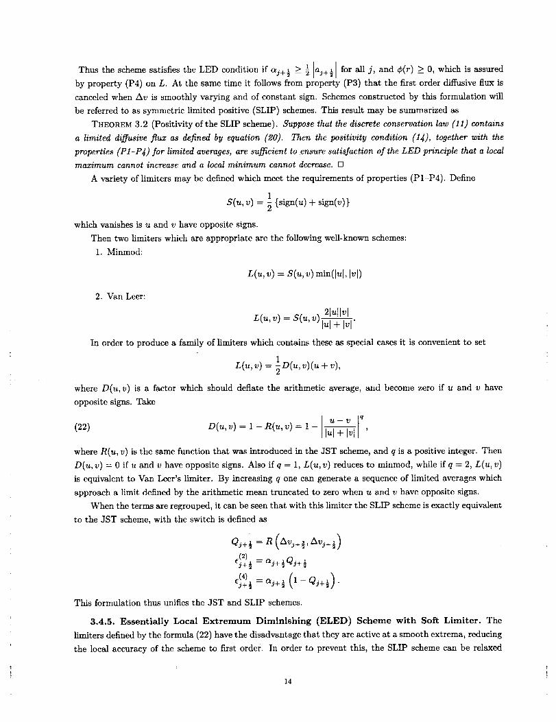
1 a_+½ for all j, and ¢(r) > 0, which is assuredThus the scheme satisfies the LED condition if aj+ ½ _> _

by property (P4) on L. At the same time it follows from property (P3) that the first order diffusive flux is

canceled when Av is smoothly varying and of constant sign. Schemes constructed by this formulation will

be referred to as symmetric limited positive (SLIP) schemes. This result may be summarized as

THEOREM 3.2 (Positivity of the SLIP scheme). Suppose that the discrete conservation law (11) contains

a limited dil)_usive flux as defined by equation (20). Then the positivity condition (14), together with the

properties (P1-P4) for limited averages, are su_cient to ensure satisfaction of the LED principle that a local

maximum cannot increase and a local minimum cannot decrease. []

A variety of limiters may be defined which meet the requirements of properties (P1-P4). Define

1 (sign(u) + sign(v)}s(u, v) =

which vanishes is u and v have opposite signs.

Then two limiters which are appropriate are the following well-known schemes:

1. Minmod:

L(u, v) = S(u, v) min(lu[, I'1)

2. Van Leer:

21ulNL(u, v) = S(u, v)1_1+ I_1"

In order to produce a family of limiters which contains these as special cases it is convenient to set

L(u, v) = 1D(u, v)(u + v),

where D(u, v) is a factor which should deflate the arithmetic average, and become zero if u and v have

opposite signs. Take

U--V q

(22) D(u, v) = l - R(u, v) = l - u + v '

where R(u, v) is the same function that was introduced in the JST scheme, and q is a positive integer. Then

D(u, v) = 0 if u and v have opposite signs. Also if q = 1, L(u, v) reduces to minmod, while if q -- 2, L(u, v)

is equivalent to Van Leer's limiter. By increasing q one can generate a sequence of limited averages which

approach a limit defined by the arithmetic mean truncated to zero when u and v have opposite signs.

When the terms are regrouped, it can be seen that with this limiter the SLIP scheme is exactly equivalent

to the JST scheme, with the switch is defined as

Qj+½ = R (Av_+],Av3+½)

e_.2)½ = ozj+½ QJ+½

e;4+)½=aS+ ½ (1-Qj+½) .

This formulation thus unifies the 3ST and SLIP schemes.

3.4.5. Essentially Local Extremum Diminishing (ELED) Scheme with Soft Limiter. The

limiters defined by the formula (22) have the disadvantage that they are active at a smooth extrema, reducing

the local accuracy of the scheme to first order. In order to prevent this, the SLIP scheme can be relaxed

14

to giveanessentiallylocalextremumdiminishing(ELED)schemewhichissecondorderaccurateat smoothextremabytheintroductionofa thresholdin the limitedaverage.ThereforeredefineD(u, v) as

U--V q(23) D(u,v) = 1- max(lui_T_],_Axr ) ,

where r = 3, q > 2. This reduces to the previous definition if lul + Ivl > eAz r.

In any region where the solution is smooth, Avj+] - Avj_ ½ is of order Ax 2. In fact if there is a smooth

extremum in the neighborhood of vj or vj+l, a Taylor series expansion indicates that Avj+], Avj+½ and

Avj_ ½ are each individually of order Ax 2, since _ = 0 at the extremum. It may be verified that second

order accuracy is preserved at a smooth extremum if q > 2. On the other hand the limiter acts in the usual

if IAvj+_ or Avj_]l > eAx r, and it may also be verified that in the limit Ax ---, 0 local maxima

i i

wayI

are non increasing and local minima are non decreasing [86]. Thus the scheme is essentially local extremum

diminishing (ELED).

The effect of the "soft limiter" is not only to improve the accuracy: the introduction of a threshold

below which extrema of small amplitude are accepted also usually results in a faster rate of convergence to

a steady state, and decreases the likelyhood of limit cycles in which the limiter interacts unfavorably with

the corrections produced by the updating scheme. In a scheme recently proposed by Venkatakrishnan a

threshold is introduced precisely for this purpose [193].

3.4.6. Upstream Limited Positive (USLIP) Schemes. By adding the anti-diffusive correction

purely from the upstream side one may derive a family of upstream limited positive (USLIP) schemes.

Corresponding to the original SLIP scheme defined by equation (20), a USLIP scheme is obtained by setting

dj+½ = aj+½ {Avj+½--L(Avj+½,Avj_½)}

if aj+ ½ > O, or

if aj+ ½ < 0. If aj+ ½ = } aj+ ½1 one recovers a standard high resolution upwind scheme in semi-discrete

form. Consider the case that aj+½ > 0 and aj_½ > O. If one sets

r + = Avj+½ r- -- Avj__

Avj_ ½' Avj_ I'

the scheme reduces to

x_- = -_ _

To assure the correct sign to satisfy the LED criterion the flux limiter must now satisfy the additional

constraint that ¢(r) <_ 2.

The USLIP formulation is essentially equivalent to standard upwind schemes [142, 185]. Both the SLIP

and USLIP constructions can be implemented on unstructured meshes [85, 86]. The anti-diffusive terms are

then calculated by taking the scalar product of the vectors defining an edge with the gradient in the adjacent

upstream and downstream cells.

3.4.7. Systems of Conservation Laws; Flux Splitting and Flux-Difference Splitting. Steger

and Warming [182] first showed how to generalize the concept of upwinding to the system of conservation

laws

(24) Ow O / w0-_+_ ( )=o

15

by the concept of flux splitting. Suppose that the flux is split as f = f+ + f- where _ and _ have

positive and negative eigenvalues. Thcn the first order upwind scheme is produced by taking the numerical

flux to be

This can be expressed in viscosity form as

hj÷ = I? + f;÷l

1 1

1 1

1: _ (fs+l + fs) - ds+½,

where the diffusive flux is

(25) di+ ½ = 1A(f+ - f-)j+½.

Roe derived the alternative formulation of flux difference splitting [163] by distributing the corrections due

to the flux difference in each interval upwind and downwind to obtain

dwjAx--dT- + (fs+1 - Ii)- + (fJ-/s-l) + --o,

where now the flux difference fi+l - fs is split. The corresponding diffusive flux is

1= -

Following Roe's derivation, let AS+ ½ be a mean value Jacobian matrix exactly satisfying the condition

(26) fs+l - fj _-Aj+½(Ws+l - ws)"

Aj+ ½ may be calculated by substituting the weighted averages

pv:Z_j+l + v_J, H = _g,+l + vr_H,(27) _ = _ + V_ _ + v:_

into the standard formulas for the Jacobian matrix A = e°-_-_.A splitting according to characteristic fields is

now obtained by decomposing Ai+ ½ as

(28) AS+ ½ = TAT -1,

where the columns of T are the cigenvectors of Aj+ ½, and A is a diagonal matrix of the eigenvalues. Now

the corresponding diffusive flux is

1AS+ ½ (Wj+l-ws),

where

AS+½1 = TIAIT -1

and IAI is the diagonal matrix containing the absolute values of the eigenvalues.

16

3.4.8. Alternative Splittings. Characteristic splitting has the advantages that it introduces the min-

imum amount of diffusion to exclude the growth of local extrema of the characteristic variables, and that

with the Roe linearization it allows a discrete shock structure with s single interior point. To reduce the

computational complexity one may replace IA] by c_I where if c_ is at least equal to the spectral radius

max [_(A)I, then the positivity conditions will still be satisfied. Then the first order scheme simply has the

scalar diffusive flux

1 A(29) dj+½ = _o_j+½ wj+½.

The JST scheme with scalar diffusive flux captures shock waves with about 3 interior points, and it has been

widely used for transonic flow calculations because it is both robust and computationaliy inexpensive.

An intermediate class of schemes can be formulated by defining the first order diffusive flux as a combi-

nation of differences of the state and flux vectors

1 , 1(30) dj+½ = _a_+½ c(wj+l - W_) + _3+½ (fj+l - fj) ,

where the factor c is included in the first term to make aj+½ and f_j+ ½ dimensionless. Schemes of this class

are fully upwind in supersonic flow if one takes a_+½ = 0 and f_j+½ - sign(M) when the absolute value of

the Mach number M exceeds 1. The flux vector f can be decomposed as

(31)

where

(32)

Then

(33)

f = uw+.fp,

(o)fp= P •

up

where 72and _ are the arithmetic averages

1 1

= _ (uj+l + us), _ = _ (wj+_ + wj).

Thus these schemes are closely related to schemes which introduce separate splittings of the convective and

pressure terms, such as the wave-particle scheme [158, 12], the advection upwind splitting method (AUSM)

[114, 197], and the convective upwind and split pressure (CUSP) schemes [85].

In order to examine the shock capturing properties of these various schemes, consider the general case

of a first order diffusive flux of the form

1(34) dj+½ = _c_j+½Bj+½ (wj+l - wj),

where the matrix Bj+ ½ determines the properties of the scheme and the scaling factor _j+ ½ is included for

convenience. All the previous schemes can be obtained by representing Bj+ ½ as a polynomial in the matrix

Aj+½ defined by equation (26). Schemes of this class were considered by Van Leer [107]. According to the

Cayley-Hamilton theorem, a matrix satisfies its own characteristic equation. Therefore the third and higher

powers of A can be eliminated, and there is no loss of generality in limiting Bj+ ½ to a polynomial of degree

2,

(35) Bj+½ =aoI + alAj+½ + a_A2+½.

17

ThecharacteristicupwindschemeforwhichBj+½ = Aj+½1 is obtained by substituting Aj+½ = TAT -1,t

A 2 = TA2T -1. Then s0, C_l, and c_2 are determined from the three equations_+½

a0+alAk+a2A_=l)_kt, k---- 1,2,3.

The same representation remains valid for three dimensional flow because Aj+½ still has only three distinct

eigenvalues u, u + c, u - c.

wL

A

j-2

!

! - wA

! !',,,X :• ;\ wR I

! !

! j+l Ii

i

j+2 !!!

FIG. 4. Shock structure for single interior point.

3.4.9. Analysis of Stationary Discrete Shocks. The ideal model of a discretc shock is illustrated

in figure (4). Suppose that WL and wR are left and right states which satisfy the jump conditions for a

stationary shock, and that the corresponding fluxes are fL = f(WL) and fR = f(WR). Since the shock is

stationary fL = fR. The ideal discrete shock has constant states WL to the left and wR to the right, and a

single point with an intermediate value WA. The intermediate value is needed to allow the discrete solution

to correspond to a true solution in which the shock wave does not coincide with an interface between two

mesh cells.

Schemes corresponding to one, two or three terms in equation (35) are examined in [87]. The analysis of

these three cases shows that a discrete shock structure with a single interior point is supported by artificial

diffusion that satisfies the two conditions that

........i.: it produces an upwind flux if the flow is determined to be supersonic through the interface

2. it satisfies a generalized eigenvalue problem for the exit from the shock of the form _

(36) (AAR -- O_ARBAR) (WR -- WA) : O,

where AAR is the linearized Jacobian matrix and BAR is the matrix defining the diffusion for the interface

AR. This follows from the equilibrium condition hRA = hRR for thc cell j + 1 in figure 4. These two

conditions are satisfied by both the characteristic scheme and also the CUSP scheme, provided that the

coefficients of convective diffusion and pressure differences are correctly balanced. Scalar diffusion does not

satisfy the first condition. In the case of the CUSP scheme (30) equation (36) reduces to

(ARA q- 1+ _] (WR--WA)=O

Thus wR - WA is an eigenvector of the Roe matrix ARA, and a'c is the corresponding eigenvalue. Since- _-_-_

the eigenvalues are u, u + c, and u - c, the only choice which leads to positive diffusion when u > 0 is u - c,

= 18 i

yieldingtherelationship

c_*c= (1 + t3)(c- u),O < u < c

This leads to a one parameter family of schemes which support the ideal shock structure. The term _(fR--fA)

contributes to the diffusion of the convective terms. Allowing for the split (31), the total effective coefficient

of convective diffusion is ac = t_*c +/T_. A CUSP scheme with low numerical diffusion is then obtained by

taking a -- IMI, leading to the coefficients illustrated in figure 5

Fro. 5. Diffusion Coe]_icients.

3.4.10. CUSP and Characteristic Schemes Admitting Constant Total Enthalpy in Steady

Flow. In steady flow the stagnation enthalpy H is constant, corresponding to the fact that the energy and

mass conservation equations are consistent when the constant factor H is removed from the energy equation.

Discrete and semi-discrete schemes do not necessarily satisfy this property. In the case of a semi-discrete

scheme expressed in viscosity form, equations (11) and (12), a solution with constant H is admitted if the

viscosity for the energy equation reduces to the viscosity for the continuity equation with p replaced by

pH. When the standard characteristic decomposition (28) is used, the viscous fluxes for p and pH which

result from composition of the fluxes for the characteristic variables do not have this property, and H is not

constant in the discrete solution. In practice there is an excursion of H in the discrete shock structure which

represents a local heat source. In very high speed flows the corresponding error in the temperature may lead

to a wrong prediction of associated effects such as chemical reactions.

The source of the error in the stagnation enthalpy is the discrepancy between the convective terms

u _ ,

pH

in the flux vector, which contain pH, and the state vector which contains pE. This may be remedied by

introducing a modified state vector

Wh _ pu .

pH

Then one introduces the linearization

fa - fL = Ah(whn - WhL).

Here Ah may be calculated in the same way as the standard Roe linearization. Introduce the weighted

19

averages defined by equation (27). Then

0 1 0 /Aa= _v+l_ v+l u z:A

"y 2 9' 3' "

-uH H u

The eigenvalues of Ah are u, )_+ and )_- where

(37) A± 3"+1 u /(3,+1 2 c2-u2±V +

Now both CUSP and characteristic schemes which preserve constant stagnation enthalpy in steady flow can

be constructed from the modified Jacobian matrix Ah [87]. These schemes also produce a discrete shock

structure with one interior point in steady flow. Then one arrives at four variations with this property, which

can conveniently be distinguished as the E- and H-CUSP schemes, and the E- and H-characteristic schemes.

3.4.11. High Order Godunov Schemes, and Kinetic Flux Splitting. Some of the most impres-

sive simulations of time dependent flows with strong shock waves have been achieved with higher order

Godunov schemes [201]. In these schemes the average value in each cell is updated by applying the inte-

gral conservation law using interface fluxes predicted from the exact or approximate solution of a Riemann

problem between adjacent cells. A higher order estimate of the solution is then reconstructed from the

cellaverages , ands!ope !im!ters are applied to the reconstruct!on: An examPle is the class of essentially

non-oscillatory (ENO) schemes, which can attain a very high order of accuracy at the cost of a substan-

tial increase in computational complexity [37, 170, 168, 169]. Methods based on reconstruction can also

be implemented on unstructured meshes [16, 15]. Recently there has been an increasing interest in kinetic

flux splitting schemes, which use solutions of the Boltzmann equation or the BGK equation to predict the

interface fluxes [50, 41, 54, 153, 202].

3.5. Multidimensional Schemes. The simplest approach to the treatment of multi-dimensional prob-

lems on structured meshes is to apply the one-dimensional construction separately in each mesh direction. On

triangulated meshes in two or three dimensions the SLIP and USLIP constructions may also be implemented

along the mesh edges [86]. A substantial body of current research is directed toward the implementation

of truly multi-dimensional upwind schemes in which the upwind biasing is determined by properties of the

flow rather than the mesh [69, 152, 109, 46, 171]. A thorough review is given by Pailliere and DeConinck in

reference [144].

Residual distribution schemes are an attractive approach for triangulated meshes. In these the residual

defined by the space derivatives is evaluated for each cell, and then distributed to the vertices with weights

which depend on the direction of convection. For a scalar conservation law the weights can be chosen to

maintain positivity with minimum cross diffusion in the direction normal to the flow. For the Euler equations

the residual can be linearized by assuming that the parameter vector with components v/-fi,_--pui, and v_H

varies linearly over the cell. Then

afj( )G

where the Jacobian matrices Aj = __z are evaluated with Roe averaging of the values of w at the vertices.

Waves in the direction n can then be expressed in terms of the eigenvectors of njAj, and a positive distribution

scheme is used for waves in preferred directions. The best choice of these directions is the subject of ongoing

2O

research, but preliminary results indicate the possibility of achieving high resolution of shocks and contact

discontinuities which are not aligned with mesh lines [144].

Hirsch and Van Ransbeeck adopt an alternative approach in which they directly construct directional

diffusive terms on structured meshes, with anti-diffusion controlled by limiters based on comparisons of

slopes in different directions [70]. They also show promising results in calculations of nozzles with multiply

reflected oblique shocks.

3.6. Discretization of the Viscous Terms. The discretization of the viscous terms of the Navier

Stokes equations requires an approximation to the velocity derivatives _ in order to calculate the tensorcgx_

a,j, equation (3). Then the viscous terms may be included in the flux balance (4). In order to evaluate the

derivatives one may apply the Gauss formula to a control volume V with the boundary S.

Iv cgui-_xj dv = Jfs uinjds

where nj is the outward normal. For a tetrahedral or hexahedral cell this gives

(38) Ou_ 1- wz_, sfaces

where _ is an estimate of the average of u, over the face. If u varies linearly over a tetrahedral cell this is

exact. Alternatively, assuming a local transformation to computational coordinates _i, one may apply the

chain rule

Here the transformation derivatives ox._ can be evaluated by the same finite difference formulas as the velocity

derivatives _ In this ease _ is exact if u is a linearly varying function.

For a cell-centered discretization (figure 6a) _-_ is needed at each face. The simplest procedure is

to evaluate N°_ in each cell, and to average -_ between the two ceils on either side of a face [95]. The

resulting discretization does not have a compact stencil, and supports undamped oscillatory modes. In a

one dimensional calculation, for example, °2u would be diseretized as ,_,.2-2,_,+,_,-2 In order to produce a4Ax 2 •

compact stencil au may be estimated from a control volume centered on each face, Using formulas (38) or

(39) [160]. This is computationally expensive because the number of faces is much larger than the number

of cells. In a hexahedral mesh with a large number of vertices the number of faces approaches three times

the number of cells.

This motivates the introduction of dual meshes for the evaluation of the velocity derivatives and the flux

balance as sketched in figure 6. The figure shows both cell-centered and cell-vertex schemes. The dual mesh

connects cell centers of the primary mesh. If there is a kink in the primary mesh, the dual cells should be

formed by assembling contiguous fractions of the neighboring primary cells. On smooth meshes comparable

results are obtained by either of these formulations [122, 123, 115]. If the mesh has a kink the cell-vertex

scheme has the advantage that the derivatives _ are calculated in the interior of a regular cell, with nocOxi

loss of accuracy.

A desirable property is that a linearly varying velocity distribution, as in a Couette flow, should produce

a constant stress and hence an exact stress balance. This property is not necessarily satisfied in general

by finite difference or finite volume schemes on curvilinear meshes. The characterization k-exact has been

proposed for schemes that are exact for polynomials of degree k. The cell-vertex finite volume scheme is

21

dual cell

i_ ii i

I

Figure 6a: Cell-

centered scheme. _ij

evaluated at vertices of

the primary mesh

Figure 6b: Cell-

vertex scheme. _rij evalu-

ated at cell centers of the

primary mesh

FIG. 6. Viscous discretizations for cell-centered and cell-vertex algorithms.

linearly exact if the derivatives are evaluated by equation (39), since then _ is exactly evaluated as aDxj

constant, leading to constant viscous stresses aij, and an exact viscous stress balance. This remains true

when there is a kink in the mesh, because the summation of constant stresses over the faces of the kinkedDu-

control volume sketched in figure 6 still yields a perfect balance. The use of equation (39) to evaluate _-_j,

however, requires the additional calculation or storage of the nine metric quantities _ in each cell, whereasOsj

equation (38) can be evaluated from the same face areas that are used for the flux balance.

In the case of an unstructured mesh, the weak form (6) leads to a natural discretization with linear

elements, in which the piecewise linear approximation yields a constant stress in each cell. This method

yields a representation which is globally correct when averaged over the cells, as is proved by energy estimates

for elliptic problems [19]. It should be noted, however, that it yields formulas that are not necessarily locally

consistent with the differential equations, if Taylor series expansions are substituted for the solution at the

vertices appearing in the local stencil. Figure 7 illustrates the discretization of the Laplacian u=_ + u_u

which is obtained with linear elements. It shows a particular triangulation such that the approximation is

locally consistent with u== + 3u_v. Thus the use of an irregular triangulation in the boundary layer may

significantly degrade the accuracy.

3

1 a l 1 c

h h

Coefl'u:ients

resulting fromlinear elcments

FIG. 7. Example of discretization u== + uuu on a triangular mesh. The discretization is locally equivalent to the approzi-ua--2_b-[-_tc o 3_d--6ueq-3Ub

mo.tiOf_ _xz -_ " h _ _ O_yy = hT_

22

Anisotropic grids are needed in order to resolve the thin boundary layers which appear in viscous flows

at high Reynolds numbers. Otherwise an excessively large number of grid cells may be required. The use of

flat tetrahedra can have an adverse effect on both the accuracy of the solution and the rate of convergence

to a steady state. This has motivated the use of hybrid prismatic-tetrahedral grids in which prismatic cells

are used in the wall regions [145]. A review of many of the key issues in the design of flow solvers for

unstructured meshes is given by Venkatakrishnan [194].

3.7. Time Stepping Schemes. If the space discretization procedure is implemented separately, it

leads to a set of coupled ordinary differential equations, which can be written in the form

(40) dwd-Y+ a(w) = 0,

where w is the vector of the flow variables at the mesh points, and R(w) is the vector of the residuals,

consisting of the flux balances defined by the space discretization scheme, together with the added dissipative

terms. If the objective is simply to reach the steady state and details of the transient solution are immaterial,

the time-stepping scheme may be designed solely to maximize the rate of convergence. The first decision that

must be made is whether to use an explicit scheme, in which the space derivatives are calculated from known

values of the flow variables at the beginning of the time step, or an implicit scheme, in which the formulas for

the space derivatives include as yet unknown values of the flow variables at the end of the time step, leading

to the need to solve coupled equations for the new values. The permissible time step for an explicit scheme

is limited by the Courant-Friedrichs-Lewy (CFL) condition, which states that a difference scheme cannot be

a convergent and stable approximation unless its domain of dependence contains the domain of dependence

of the corresponding differential equation. One can anticipate that implicit schemes will yield convergence

in a smaller number of time steps, because the time step is no longer constrained by the CFL condition.

Implicit schemes will be efficient, however, only if the decrease in the number of time steps outweighs the

increase in the computational effort per time step consequent upon the need to solve coupled equations. The

prototype implicit scheme can be formulated by estimating -_ at t + #At as a linear combination of R(w n)

and R(w'_+l). The resulting equation

can be lineaxized as

w n+l =w _-At{(1-#)R(w n)+#R(w _+1)}

If one sets # -- 1 and lets At --, _ this reduces to the Newton iteration, which has been successfully used

in two-dimensional calculations [192, 59]. In the three-dimensional case with, say, an N × N × N mesh,

the bandwidth of the matrix that must be inverted is of order N _. Direct inversion requires a number of

operations proportional to the number of unknowns multiplied by the square of the bandwidth of the order

of N 7. This is prohibitive, and forces recourse to either an approximate factorization method or an iterative

solution method.

Alternating direction methods, which introduce factors corresponding to each coordinate, are widely used

for structured meshes [21, 154]. They cannot be implemented on unstructured tetrahedral meshes that do

not contain identifiable mesh directions, although other decompositions are possible [66, 116]. If one chooses

to adopt the iterative solution technique, the principal alternatives are variants of the Gauss-Seidel and

Jacobi methods. A symmetric Gauss-Seidel method with one iteration per time step is essentially equivalent

23

to anapproximatelower-upper(LU) factorizationof the implicitscheme[94,137,36,205].Ontheotherhand,theJacobimethodwith a fixednumberof iterationspertimestepreducesto a multistageexplicitscheme,belongingto thegeneralclassofRunge-Kuttaschemes[38].Schemesofthis typehaveprovedveryeffectivefor widevarietyofproblems,andtheyhavetheadvantagethat theycanbeappliedequallyeasilyonbothstructuredandunstructuredmeshes[93,78,80,161].

If onereducesthelinearmodelproblemcorrespondingto (40)to anordinarydifferentialequationbysubstitutinga Fouriermode_ -- e_vx_, theresultingFouriersymbolhasanimaginarypartproportionaltothewavespeed,andanegativerealpartproportionaltothediffusion.Thusthetimesteppingschemeshouldhavea stabilityregionwhichcontainsasubstantialintervalofthenegativerealaxis,aswellasan intervalalongtheimaginaryaxis.Toachievethis it paysto treattheconvectiveanddissipativetermsin adistinctfashion.Thustheresidualis splitas

R(w) ----Q(w) + D(w),

where Q(w) is the convective part and D(w) the dissipative part. Denote the time level nat by a superscript

n. Then the multistage time stepping scheme is formulated as

W(n+l, 0) _ W n

=

wn+ 1 _ w(n+l,rn),

where the superscript k denotes the k-th stage, c_m = 1, and

Q(0) = Q (w"), D (°) = D (w")

D (k) = 3kD (W (n+l'k)) "J-(1- flk)D (k-l).

The coefficients ak are chosen to maximize the stability interval along the imaginary axis, and the coefficients

flk are chosen to increase the stability interval along the negative real axis•

These schemes do not fall within the standard framework of Runge-Kutta schemes, and they have much

larger stability regions [80]. Two schemes which have been found to be particularly effective are tabulated

below. The first is a four-stage scheme with two evaluations of dissipation. Its coefficients are

(41)

1_1 = _ 31 = 1

5a3 = 6 3'3 = 0

c_4=1 /5',,=0

The second is a five-stage scheme with three evaluations of dissipation. Its coefficients are

(42)

oq=¼ /31----1

/32=0-3 = /33= 0.56 ._4=½ /34=o

(_5=1 135=0.44

24

3.8. Multigrid Methods.

3.8.1. Acceleration of Steady Flow Calculations. Radical improvements in the rate of convergence

to a steady state can be realized by the multigrid time-stepping technique. The concept of acceleration by the

introduction of multiple grids was first proposed by Fedorenko [57]. There is by now a fairly well-developed

theory of multigrid methods for elliptic equations based on the concept that the updating scheme acts as a

smoothing operator on each grid [28, 62]. This theory does not hold for hyperbolic systems. Nevertheless,

it seems that it ought to be possible to accelerate the evolution of a hyperbolic system to a steady state

by using large time steps on coarse grids so that disturbances will be more rapidly expelled through the

outer boundary. Various multigrid time-stepping schemes designed to take advantage of this effect have

been proposed [136, 77, 64, 81, 34, 9, 67]

One can devise a multigrid scheme using a sequence of independently generated coarser meshes by

eliminating alternate points in each coordinate direction. In order to give a precise description of the

multigrid scheme, subscripts may be used to indicate the grid. Several transfer operations need to be

defined. First the solution vector on grid k must be initialized as

W(k O) = Tk,k-lWk-l_

where wk-1 is the current value on grid k - 1, and Tk,k-1 is a transfer operator. Next it is necessary to

transfer a residual forcing function such that the solution grid k is driven by the residuals calculated on grid

k - 1. This can be accomplished by setting

F (o)lPk = Qk,k-lRk-1 (Wk-1) -- Rk [Wk ],

where Qk,k-1 is another transfer operator. Then Rk(Wk) is replaced by Rk(Wk) + Pk in the time- stepping

scheme. Thus, the multistage scheme is reformulated as

The result w(km) then provides the initial data for grid k + 1. Finally, the accumulated correction on grid

k has to be transferred back to grid k - 1 with the aid of an interpolation operator Ik-l,_. With properly

optimized coefficients multistage time-stepping schemes can be very efficient drivers of the multigrid process.

A W-cycle of the type illustrated in Figure 8 proves to be a particularly effective strategy for managing the

work split between the meshes. In a three-dimensional case the number of cells is reduced by a factor of

eight on each coarser grid. On examination of the figure, it can therefore be seen that the work measured in

units corresponding to a step on the fine grid is of the order of

1 + 2/8 -t- 4/64 +... < 4/3,

and consequently the very large effective time step of the complete cycle costs only slightly more than a

single time step in the fine grid.

This procedure has proved extremely successful for the solution of the inviseid Euler equations, but less

effective in calculations of turbulent viscous flows at high Reynolds numbers using the Reynolds averaged

Navier Stokes equations. These require highly anisotropic grids with very fine mesh intervals normal to the

wall to resolve the boundary layers. While simple multigrid methods still yield fast initial convergence, they

25

Figure 8a: 3 Levels.

Figure 8b: 4 Levels.

Figure 8c: 5 Levels.

FIc. 8. Multigrid W-cycle for managing the grid calculation. E, evaluate the change in the flow for one step; T, transfer

the data without updating the solution.

tend to slow down as the calculation proceeds to a low asymptotic rate. This has motivated the introduction

of semi-coarsening and directional coarsening methods [132, 133, 3, 4, 5, 148, 149].

The multigrid method can be applied on unstructured meshes by interpolating between a sequence

of separately generated meshes with progressively increasing cell sizes [91, 126, 127, 146]. It is not easy

to generate very coarse meshes for complex configurations. An alternative approach, which removes this

difficulty, is to automatically generate successively coarser meshes by agglomerating control volumes or by

collapsing edges. This approach yields comparable rates of convergence and has proved to be quite robust

[101,102, 128, 42].

3.8.2. Multigrid Implicit Schemes for Unsteady Flow. Time dependent calculations are needed

for a number of important applications, such as flutter analysis, or the analysis of the flow past a helicopter

rotor, in which the stability limit of an explicit scheme forces the use of much smaller time steps than would

be needed for an accurate simulation. In this situation a multigrid explicit scheme can be used in an inner

iteration to solve the equations of a flflly implicit time stepping scheme [84].

Suppose that (40) is approximated as

Dtw n+l + R(w n+l) = O.

Here Dt is a k th order accurate backward difference operator of the form

Dt = _'_ q=l

where

h-w n+l _ w n+l _ w n.

26

Applied to the linear differential equation

dw-- _OI.Wdt

the schemes with k -- 1, 2 are stable for all aAt in the left half plane (A-stable). Dahlquist has shown that

A-stable linear multi-step schemes axe at best second order accurate [44]. Gear however, has shown that the

schemes with k _< 6 are stiffly stable [58], and one of the higher order schemes may offer a better compromise

between accuracy and stability, depending on the application.

Equation (40) is now treated as a modified steady state problem to be solved by a multigrid scheme

using variable local time steps in a fictitious time t*. For example, in the case k -- 2 one solves

Ow

Ot_ + R* (w) = O,

where

3 2wn 1 n-1R'(w) = h-_w + R(w) - At + 5h_ _ '

and the last two terms are treated as fixed source terms. The first term shifts the Fourier symbol of the

equivalent model problem to the left in the complex plane. While this promotes stability, it may also require

a limit to be imposed on the magnitude of the local time step At* relative to that of the implicit time step

At. This may be relieved by a point-implicit modification of the multi-stage scheme [129]. In the case of

problems with moving boundaries the equations must be modified to allow for movement and deformation

of the mesh.

This method has proved effective for the calculation of unsteady flows that might be associated with

wing flutter [6, 7] and also in the calculation of unsteady incompressible flows [22]. It has the advantage that

it can be added as an option to a computer program which uses an explicit multigrid scheme, allowing it to be

used for the efficient calculation of both steady and unsteady flows. A similar approach has been successfully

adopted for unsteady flow simulations on unstructured grids by Venkatakrishnan and Mavriplis [195].

3.9. Preconditioning. Another way to improve the rate of convergence to a steady state is to mul-

tiply the space derivatives in equation (1) by a preconditioning matrix P which is designed to equalize the

eigenvalues, so that all the waves can be advanced with optimal time steps. A symmetric preconditioner

which equalizes the eigenvalues has been proposed by Van Leer [110]. When the equations are written in

stream-aligned coordinates this has the form

p

_M 2 -_M 0 0 0

-_M _+1 0 0 0

0 0 T 0 0

0 0 0 "r 0

0 0 0 0 1

where

_=T= vfl-M 2, if M< 1

]_=v/1-M2,r=V/1 M2 , if M>I

Turkel has proposed an asymmetric preconditioner which has also proved effective, particularly for flow at

low Mach numbers [191]. The use of these preconditioners can lead to instability at stagnation points where

there is a zero eigenvalue which cannot be equalized with the eigenvalues :kc.

27

The preconditioners of Van Leer and Turkel do not take account of the effect of differences in the

mesh intervals in the different coordinate directions. The need to resolve the boundary layer generally

compels the introduction of mesh cells with very high aspect ratios near the boundary, and these can lead

to a severe reduction in the rate of convergence to a steady state. Allmaras has analyzed explicit and

implicit Jacobi-based preconditioners which include the influence of the mesh intervals [3, 4, 5]. Using

a block-Jacobi preconditioner with coarsening only in the direction normal to the wall, Pierce has recently

obtained impressive results on viscous flows with high aspect ratio grids [148, 149]. Mavriplis has successfully

combined block preconditioners with line solvers to accelerate the convergence of viscous flow solutions on

highly stretched unstructured grids [125].

An alternative approach has recently been proposed by Ta'asan [186], in which the equations are written

in a canonical form which separates the equations describing acoustic waves from those describing convection.

In terms of the velocity components u, v and the vorticity w, temperature T, entropy s and total enthalpy

H, the equations describing steady two-dimensional flow can be written as

D1 02 0 0 0

o o -1 0 0-_ a-_

c2 D 10 0 -q _(_ 3 _D3

0 0 0 TpQ 0

0 0 0 0 pQ

U

V

tO

8

H

=0

where

and

D1 = .c 2 - u 2. - uv

D2 = .c 2 - U2) cly - uv

0 0

D3 = V-_x - u _-_Y0 0

Q = + Y

q2 : tt2 .._ V 2"

Here the first three equations describe an elliptic system if the flow is subsonic, while the remaining equations

are convective. Now separately optimized multigrid procedures are used to solve the two sets of equations,

which are essentially decoupled. An alternative approach to the optimal splitting of the flow equations into

convective and acoustic parts has been developed by Sidilkover [172, 162].

3.10. High Order Schemes and Mesh Refinement. The need both to improve the accuracy of

computational simulations, and to assure known levels of accuracy is the focus of ongoing research. The

main routes to improving the accuracy are to increase the order of the discrete scheme, and reduce the mesh

interval. High order difference methods are most easily implemented on Cartesian, or at least extremely

smooth grids. The expansion of the stencil as the order is increased leads to the need for complex boundary

conditions. Compact schemes keep the stencil as small as possible [157, 112, 33]. On simple domains,

spectral methods are particularly effective, especially in the case of periodic boundary conditions, and can

be used to produce exponentially fast convergence of the error as the mesh interval is decreased [139, 32]. A

28

compromise is to divide the field into subdomains and introduce high order elements. This approach is used

in the spectral element method [100].

High order difference schemes and spectral methods have proven particularly useful in direct Navier-

Stokes simulations of transient and turbulent flows. High order methods are also beneficial in computational

hero-acoustics, where it is desired to track waves over long distances with minimum error. If the flow contains

shock waves or contact discontinuities, the ENO method may be used to construct high order non-oscillatory

schemes.

In multi-dimensional flow simulations, global reduction of the mesh interval can be prohibitively expen-

sive, motivating the use of adaptive mesh refinement procedures which reduce the local mesh width h if there

is an indication that the error is too large [25, 45, 117, 71, 155, 111, 147]. In such h-refinement methods,

simple error indicators such as local solution gradients may be used. Alternatively, the discretization error

may be estimated by comparing quantities calculated with two mesh widths, say on the current mesh and a

coarser mesh with double the mesh interval. Procedures of this kind may also be used to provide a posteriori

estimates of the error once the calculation is completed.

This kind of local adaptive control can also be applied to the local order of a finite element method

to produce a p-refinement method, where p represents the order of the polynomial basis functions. Finally,

both h- and p- refinement can be combined to produce an h-p method in which h and p are locally optimized

to yield a solution with minimum error [138]. Such methods can achieve exponentially fast convergence, and

are well established in computational solid mechanics.

4. Current Status of Numerical Simulation. This section presents some representative numerical

results which confirm the properties of the algorithms which have been reviewed in the last section. These

have been drawn from the work of the author and his associates. They also illustrate the kind of calculation

which can be performed in an industrial environment, where rapid turn around is important to allow the

quick assessment of design changes, and computational costs must be limited.

4.1. One dimensional shock. In order to verify the discrete structure of stationary shocks, calcu-

lations were performed for a one dimensional problem with initial data containing left and right states

compatible with the Rankine Hugoniot conditions. An intermediate state consisting of the arithmetic av-

erage of the left and right states was introduced at a single cell in the center of the domain. With this

intermediate state the system is not in equilibrium, and the time dependent equations were solved to find

an equilibrium solution with a stationary shock wave separating the left and right states. Table 1 shows the

result for a shock wave at Much 20. This calculation used the H-CUSP scheme, which allows a solution with

constant stagnation enthalpy. The SLIP-JST construction was used with the limiter defined by equation

(23), and q - 3. The table shows the values of p, u, H, p, M and the entropy S -- log _ - log (p___L).

A perfect one point shock structure is displayed. The entropy is zero to 4 decimal places upstream of the

shock, exhibits a slight excursion at the interior point, and is constant to 4 decimal places downstream of the

shock. It may be noted that the mass, momentum and energy of the initial data are not compatible with the

final equilibrium state. According to conservation arguements the total mass, momentum and energy must

remain constant if the outflow flux fn remains equal to the inflow flux fL. Therefore fR must bc allowed

to vary according to an appropriate outflow boundary condition to allow the total mass, momentum and

energy to be adjusted to values compatible with equilibrium:

4.2. Euler Calculations for Airfoils and Wings. The results of transonic flow calculations for two

well known airfoils, the RAE 2822 and the NACA 0012, are presented in figures (21-23). The H-CUSP

29

I p H p M

19 1.0000 283.5000 1.0000 20.0000

20 1.0000 283.5000 1.0000 20.0000

21 1.0000 283.5000 1.0000 20.0000

22 4.1924 283.4960 307.4467 0.7229

23 5.9259 283.4960 466.4889 0.3804

24 5.9259 283.4960 466.4889 0.3804

25 5.9259 283.4960 466.4889 0.3804

TABLE 1

Shock Wave at Mach 20

scheme was again used with the SLIP-JST construction. The limiter defined by equation (23) was used with

q -- 3. The 5 stage time stepping scheme (42) was augmented by the multigrid scheme described in section

4.2 to accelerate convergence to a steady state. The equations were discretized on meshes with O-topology

extending out to a radius of about 100 chords. In each case the calculations were performed on a sequence

of successively finer meshes from 40x8 to 320x64 cells, while the multigrid cycles on each of these meshes

descended to a coarsest mesh of 10x2 ceils. Figures 21-23 show the final results on 320x64 meshes for the

RAE 2822 airfoil at Mach .75 and 3° angle of attack, and for the NACA 0012 airfoil at Mach .8 and 1.25 °

angle of attack, and also at Mach .85 and 1° angle of attack. In the pressure distributions the pressure

coefficient Cp = _ is plotted with the negative (suction) pressures upward, so that the upper curve

represents the flow over the upper side of a lifting airfoil. The convergence histories show the mean rate

of change of the density, and also the total number of supersonic points in the flow field, which provides

a useful measure of the global convergence of transonic flow calculations such as these. In each case the

convergence history is shown for 100 cycles, while the pressure distribution is displayed after a sufficient

number of cycles for its convergence. The pressure distribution of the RAE 2822 airfoil converged in only 25

cycles. Convergence was slower for the NACA 0012 airfoil. In the case of flow at Mach .8 and 1.25 ° angle of

attack, additional cycles were needed to damp out a wave downstream of the weak shock wave on the lower

surface. __ :_ : __ : : ::: __:_: : :: : ..... :

As a further check on accuracy the drag coefficient should be zero in subsonic flow, or in shock free

transonic flow. Table 2 shows the computed drag coefficient on a sequence of three meshes for three examples.

The first two are subsonic flows over the RAE 2822 and NACA 0012 airfoils at Mach .5 and 3° angle of

attack. The third is the tiow over the shock free Korn airfoil at its design point of Mach .75 and 0 ° angle of

attack. In all three cases the drag coefficient is calculated to be zero to four digits on a 160x32 mesh.

Mesh

40x8

80x16

160x32

RAE 2822 NACA 0012 Korn Airfoil

Mach .50 Mach .50 Mach .75

a 3° oe3° o_0°

.0062 .0047 .0098

.0013 .0008 .0017

.0000 .0000 .0000

TABLE 2

Dra 9 CoeJ]icient on a sequence of meshes

3O

As a further test of the performance of the H-CUSP scheme, the flow past the ONERA M6 wing was

calculated on a mesh with C-H topology and 192x32x48 -- 294912 cells. Figure 24 shows the result at Mach

.84 and 3.06 ° angle of attack. This again verifies the non-oscillatory character of the solution, and the sharp

resolution of shock waves. In this case 50 cycles were sufficient for convergence of the pressure distributions.

Figure 9 shows a calculation of the Northrop YF23 by R.J. Busch, Jr., who used the author's FLO57

code to solve the Euler equations [30]. Although an inviscid model of the flow was used, it can be seen that

the simulations are in good agreement with wind tunnel measurements both at Mach .90, with angles of

attack of 0, 8 and 16 degrees, and at Mach 1.5 with angles of attack of 0, 4 and 8 degrees. At a high angle of

attack the flow separates from the leading edge, and this example shows that in situations where the point

of separation is fixed, an inviscid model may still produce a useful prediction. Thus valuable information for

the aerodynamic design could be obtained with a relatively inexpensive computational model.

FIc. 9. Comparison of Experimental and Computed Drag Rise Curve for the YF-$3 (Supplied by R. J. Bush Jr.)

The next figures show the results of calculations using the AIRPLANE code developed by T.J. Baker

and the author, to solve the Euler equations on an unstructured mesh. This provides the flexibility to

treat arbitrarily complex configurations without the need to spend months developing an acceptable mesh.

Figures 10 and 11 show calculations for supersonic transport configurations which were performed by Susan

Cliff. The agreement with experimental data is quite good, and it has also been possible to predict the

sonic boom signature [39]. Figure 12 shows an Euler calculation for the McDonnell Douglas MD11 with flow

through the engine nacelles, using 348407 mesh points of 2100466 tetrahedra. This calculation takes 4 hours

on an IBM 590 workstation. A parallel version of the code has been developed in collaboration with W.S.

Chen, and the same calculation can be performed in 16 minutes using 16 processors of an IBM SP2. The

parallel speed-up for the MDll is shown in table 3.

31

LL. ....

Force C_ff_clea_, M_h 2.L

o_

Soaic Boom Pr_ic_ion_ M_b 2 5

FIG. t0. Comparison of Experimental and Calculated Results for a HSCT Configuration

FIG. 11. Pressure Contours and Sonic Boom on a Representative HSCT Configuration

4.3. Viscous Flow Calculations• The next figures show viscous simulations based on the solution of

the Reynolds averaged Navier Stokes equations with turbulence models. Figure 13 shows a two-dimensional

calculation for the RAE 2822 airfoil by L. Martinelli. The vertical axis represents the negative pressure

coefficient, and there is a shock wave half way along the upper surface. This example confirms that in the

absence of significant shock induced separation, simulations performed on a sufficiently fine mesh (512 x 64)

can produce excellent agreement with experimental data. Figure 20 shows a simulation of the McDonnell-

Douglas F18 performed by R.M. Cummings, Y.M. Rizk, L.B. Schiff and N.M. Chaderjian at NASA Ames

[43]. They used a multiblock mesh with about 900000 mesh points. While this is probably not enough for

32

No. of Nodes Seconds/Cycle Speedup

1 36.03 1.00

2 18.11 1.99

4 9.11 3.96

8 4.66 7.73

16 2.39 15.08

TABLE 3

AIRPLANE Parallel Performance on the SP_, MD-11 Model

an accurate quantitative prediction, the agreement with both the experimental data and the visualization

are quite good.

AIRPLA_E MDI 1 CPAculation

FIG. 12. Computed Pressure Field for a McDonnell Douglas MD11

Figure 14 shows an unsteady flow calculation for a pitching airfoil performed by 3. Alonso using the

code UFLO82, which he jointly developed with L. Martinelli and the author [7]. This uses the multigrid

implicit scheme described in Section 3.7.2 which allows the number of time steps to be reduced from several

thousand to 36 per pitching cycle. The agreement with experimental data is quite good.

4.4. Ship Wave Resistance calculations. Figures 51-53 show the results of an application of the

same multigrid finite volume techniques to the calculation of the flow past a naval frigate, using a code which

was developed by J. Farmer, L. Martinelli and the author [56]. The mesh was adjusted during the course

of the calculation to conform to the free surface in order to satisfy the exact non-linear boundary condition,

while artificial compressibility was used to reat the incompressible flow equations.

5. Aerodynamic Shape Optimization.

5.1. Optimization and Design. Traditionally the process of selecting design variations has been

carried out by trial and error, relying on the intuition and experience of the designer. With currently

available equipment the turn around for numerical simulations is becoming so rapid that it is feasible to

examine an extremely large number of variations. It is not at all likely that repeated trials in an interactive

design and analysis procedure can lead to a truly optimum design. In order to take full advantage of the

possibility of examining a large design space the numerical simulations need to be combined with automatic

33

t

__ Compu_io,

RAE2822 6 .225

14ACHO.T29 AJ_HA 2.310

GR_ SI_ NCYC 75 F.F__OOOE._0

F]c. 13. Two-Dimensional Turbulent Viscous Calculation (by Luigi Martinelli)

search and optimization procedures. This can lead to automatic design methods which will fully realize the

potential improvements in aerodynamic efficiency.

The simplest approach to optimization is to define the geometry through a set of design parameters,

which may, for example, be the weights a, applied to a set of shape functions b_(x) so that thc shape is

represented as

y(x) = F_,

Then a cost function I is selected which might, for example, be the drag coefficient at a final lift coefficient,OI

and I is regarded as a function of the parameters ai. The sensitivities _ may now be estimated by making

a small variation 5c_i in each design parameter in turn and recalculating the flow to obtain the change in I.

Then

aI I(a_ + 5a_) - I(a+)

Oai 5ai

DIThe gradient vector ga may now be used to determine a direction of improvement. The simplest procedure

is to make a step in the negative gradient direction by setting

OIO_ n+l = Ot n -- _--_

so that to first order

oIT 5a ,k �)IT OII+SI=I-_ =I- Oa Oa"

34

:St 7 i/7,tit

FIG. 14. Mach Number Contours. Pi_ching Airfoil Case. Re = 1.0 x 106, M_ ---- 0.796, Kc ----0.202.

More sophisticated search procedures may be used such as quasi-Newton methods, which attempt to estimate

the second derivative _°'l of the cost flmction from changes in the gradient _°I in successive optimization

steps. These methods also generally introduce line searches to find the minimum in the search direction

which is defined at each step. The main disadvantage of this approach is the need for a number of flow

calculations proportional to the number of design variables to estimate the gradient. The computational

costs can thus become prohibitive as the number of design variables is increased.

An alternative approach is to cast the design problem as a search for the shape that will generate the

desired pressure distribution. This approach recognizes that the designer usually has an idea of the the

kind of pressure distribution that will lead to the desired performance. Thus, it is useful to consider the

inverse problem of calculating the shape that will lead to a given pressure distribution. The method has the

advantage that only one flow solution is required to obtain the desired design. Unfortunately, a physically

realizable shape may not necessarily exist, unless the pressure distribution satisfies certain constraints. Thus

the problem must be very carefully formulated; otherwise it may be ill posed.

The difficulty that the target pressure may be unattainable may be circumvented by treating the inverse

problem as a special case of the optimization problem, with a cost function which measures the error in the

solution of the inverse problem. For example, if Pd is the desired surface pressure, one may take the cost

function to be an integral over the the body surface of the square of the pressure error,

I = _ (p - pd)2dB,

or possibly a more general Sobolev norm of the pressure error. This has the advantage of converting a

possibly ill posed problem into a well posed one. It has the disadvantage that it incurs the computational

costs associated with optimization procedures.

5.2. Application of Control Theory. In order to reduce the computational costs, it turns out that

there are advantages in formulating both the inverse problem and more general aerodynamic problems

35

t'_ /

FIG. 15. Contours of Surface Wave Elevation for a Combatant Ship

/ ..'5;;-":-', ..5""

FIG. 16. Contours of Surface Wave Elevation Near the Transom Stern

within the framework of the mathematical theory for the control of systems governed by partial differential

equations [ii3]] A wing, for example, is a device to produce lift by controlling the flow, and its design

can be regarded as a problem in the optimal control of the flow equations by variation of the shape of the

boundary. If the boundary shape is regarded as arbitrary within some requirements of smoothness, then

the full generality of shapes cannot be defined with a finite number of parameters, and one must use the

concept of the Frechet derivative of the cost with respect to a function. Clearly, such a derivative cannot be

determined directly by finite differences of the design parameters because there are now an infinite number of

these. Using techniques of control theory, however, the gradient can be determined indirectly by solving an

adjoint equation which has coefficients defined by the solution of the flow equations. The cost of solving the

adjoint equation is comparable to that of solving the flow equations. Thus the gradient can be determined

with roughly the computational costs of two flow solutions, independently of the number of design variables,

which may be infinite if the boundary is regarded as a free surface. The underlying concepts are clarified by

the following abstract description of the adjoint method. For flow about an airfoil or wing, the aerodynamic

36

FIG. 17. Pressure Contours in the Bow Region

properties which define the cost function are functions of the flow-field variables (w) and the physical location

of the boundary, which may be represented by the function Y', say. Then

and a change in _" results in a change

I = I(w,.T'),

ro.,q ro.,- l(43) 6I = Law j, a,_+ Lo.r j _

in the cost function. Here, the subscripts I and // are used to distinguish the contributions due to the

variation 6w in the ftow solution from the change associated directly with the modification _9r in the shape.

This notation assists in grouping the numerous terms that arise during the derivation of the full Navier-

Stokes adjoint operator, outlined in the next section, so that the basic structure of the approach as it is

sketched in the present section can easily be recognized.

Suppose that the governing equation R which expresses the dependence of w and f within the flowfield

domain D can be written as

(44) R (w, _) = O.

Then 8w is determined from the equation

i II

Since the variation _R is zero, it can be multiplied by a Lagrange Multiplier ¢ and subtracted from the

variation _I without changing the result. Thus equation (43) can be replaced by

_I = tglT6w oIT __ _yT OR OR 6_')

Choosing ¢ to satisfy the adjoint equation

(47) _ ¢ = 0-_

37

thefirst termiseliminated,andwefind that

(48)

where

oIT _)T[ OR]g- a7 "

The advantage is that (48) is independent of 5w, with the result that the gradient of I with respect to an

arbitrary number of design variables can be determined withou;the need for additional flow-field evaluations.

In the case that (44) is a partial differential equation, the adjoint equation (47) is also a partial differential

equation and determination of the appropriate boundary conditions requires careful mathematical treatment.

In reference [82] the author derived the adjoint equations for transonic flows modelled by both the

potential flow equation and the Euler equations. The theory was developed in terms of partial differential

equations, leading to an adjoint partial differential equation. In order to obtain numerical solutions both

the flow and the adjoint equations must be discretized. The control theory might be applied directly to the

discrete flow equations which result from the numerical approximation of the flow equations by finite element,

finite volume or finite difference procedures. This leads directly to a set of discrete adjoint equations with a

matrix which is the transpose of the Jacobian matrix of the full set of discrete nonlinear flow equations. On

a three-dimensional mesh with indices i, j, k the individual adjoint equations may be derived by collecting

together all the terms multiplied by the variation (_wij,k of the discrete flow variable w_d,k. The resulting

discrete adjoint equations represent a possible discretization of the adjoint partial differential equation. If

these equations are solved exactly they can provide an exact gradient of the inexact cost function which

results from the discretization of the flow equations. The discrete adjoint equations derived directly from the

discrete flow equations become very complicated when the flow equations are discretized with higher order

upwind biased schemes using flux limiters. On the other hand any consistent discretization of the adjoint

partial differential equation will yield the exact gradient in the limit as the mesh is refined. The trade-off

between the complexity of the adjoint discretization, the accuracy of the resulting estimate of the gradient,

and its impact on the computational cost to approach an optimum solution is a subject of ongoing research.

The true optimum shape belongs to an infinitely dimensional space of design parameters. One motivation

for developing the theory for the partial differential equations of the flow is to provide an indication in

principle of how such a solution could be approached if sufficient computational resources were available.

Another motivation is that it highlights the possibility of generating ill posed formulations of the problem.

For example, if one attempts to calculate the sensitivity of the pressure at a particular location to changes

in the boundary shape, there is the possibility that a shape modification could cause a shock wave to pass

over that location. Then the sensitivity could become unbounded. The movement of the shock, however,

is continuous as the shape changes. Therefore a quantity such as the drag coefficient, which is determined

by integrating the pressure over the surface, also depends continuously on the shape. The adjoint equation

allows the sensitivity of the drag coefficient to be determined without the explicit evaluation of pressure

sensitivities which would be ill posed.

The discrete adjoint equations, whether they are derived directly or by discretization of the adjoint

partial differential equation, are linear. Therefore they could be solved by direct numerical inversion. In

three-dimensional problems on a mesh with, say, n intervals in each coordinate direction, the number of

unknowns is proportional to n 3 and the bandwidth to n2. The complexity of direct inversion is proportional

to the number of unknowns multiplied by the square of the bandwidth, resulting in a complexity proportional

38

to n r. The cost of direct inversion can thus become prohibitive as the mesh is refined, and it becomes more

efficient to use iterative solution methods. Moreover, because of the similarity of the adjoint equations to

the flow equations, the same iterative methods which have been proved to be efficient for the solution of the

flow equations are efficient for the solution of the adjoint equations.

The control theory formulation for optimal aerodynamic design has proved effective in a variety of

applications [83, 74, 159]. Pironneau has studied the use of control theory for optimal shape design of

systems governed by elliptic equations [151], and more recently the Navier-Stokes equations, and also wave

reflection problems [150]. The adjoint equations have also been used by Baysal and Eleshaky [20], and

by Ta'asan, Kuruvila and Salas [187], who have implemented a one shot approach in which the constraint

represented by the flow equations is only required to be satisfied by the final converged solution. In their

work, computational costs are also reduced by applying multigrid techniques to the geometry modifications as

well as the solution of the flow and adjoint equations. Adjoint methods have been applied to incompressible

viscous flow problems by Cabuk and Modi [31, 72] and by Desai and Ito [49]. Recent applications of adjoint

methods on unstructured meshes include the work of Anderson and Venkatakrishnan [10], and Elliot and

Peraire [53].

5.3. Three-Dimenslonal Design using the Compressible Navler-Stokes Equations. In order

to illustrate the application of control theory to aerodynamic design problems, this section treats three-

dimensional wing design using the compressible Navier Stokes equations to model the flow. In comparison

with incompressible viscous flow, the adjoint equations contain numerous extra terms which arise from the

variation of the energy equation. In order to simplify the calculation of the effect of shape changes it is

convenient to introduce a body-fitted coordinate system, so that the flow and adjoint equations are solved

in a fixed computational domain. Suppose that the transformation to computational coordinates (_1, _2, _a)

is defined by the metrics

K1=[o ,1Kij = (K) , ,j Lcgxj j .

The Navier-Stokes equations (1-3) can then be written in the computational domain as

(a9) 0 (aw)o--7-- + R(w) = 0 in V,

where

0 (f, - Fv,)(50) =

where the inviscid and viscous flux contributions are now defined with respect to the computational cell

faces by F_ = S_jfj and F_,_ --- S_jf,,j, and the quantity S_j -.= JK_ 1 is used to represent the projection of the

_i cell face along the xj axis. For convenience, the coordinates _i describing the fixed computational domain

are chosen so that each boundary conforms to a constant value of one of these coordinates. Variations in

the shape then result in corresponding variations in the mapping derivatives defined by Kij.

Suppose that the performance is measured by a cost function

I -- M (w,S) dB, + fv l='(w,S) dD,,

containing both boundary and field contributions where dB_ and dD_ are the surface and volume elements in

the computational domain. In general, .Ad and T_will depend on both the flow variables w and the metrics

39

S defining the computational space. The design problem is now treated as a control problem where the

boundary shape represents the control function, which is chosen to minimize I subject to the constraints

defined by the flow equations (49). A shape change produces a variation in the flow solution _w and the

metrics _S which in turn produce a variation in the cost function

(51)JB J_

Here

(52) _, = [7_]_ _w + _Th_,

where we continue to use the subscripts I and H to distinguish between the contributions associated with

the variation of the flow solution 6w and those associated with the metric variations 6S. Thus [.h_]j and

a]_ and a_, with the metrics fixed, while 6A/IH and _IPu represent the contribution of the[_w] I represent -g-6-

metric variations _S to _A_ and _P.

In the steady state, the constraint equation (53) specifies the variation of the state vector _w by

O

(53) 0_--_5(Fi - F_,,) = O.

Here _Fi and 6Fvi can also be split into contributions associated with _w and 6S using the notation

(54)

The inviscid contributions are easily evaluated as

of_[F,_] I = aqTww, _F._u = _Sofj.

The details of the viscous contributions are complicated by the additional level of derivatives in the stress

and heat flux terms.

Multiplying by a co-state vector ¢, which will play an analogous role to the Lagrange multiplier intro-

duced in equation (46), and integrating over the domain produces

(55) /z_ _T £ _ (Fi - F_i) d_, =0.

Assuming that ¢ is differentiable this may be integrated by parts to give

(56)

This equation results directly from taking the variation of the weak form of the flow equations, where ¢ is

taken to be an arbitrary differentiable test function. Since the left hand expression equals zero, it may be

subtracted from the variation in the cost function (51) to give

_I = ._ [aM - niCT _ (Fi - F,_i)] dB_

4o

Now.since¢ is anarbitrarydifferentiablefunction,it maybechosenin sucha waythat 5I no longer

depends explicitly on the variation of the state vector _w. The gradient of the cost function can then be

evaluated directly from the metric variations without having to recompute the variation gw resulting from

the perturbation of each design variable.

Comparing equations (52) and (54), the variation _w may be eliminated from (57) by equating all field

terms with subscript "/" to produce a differential adjoint system governing ¢

(58) °¢TO¢i [Fi_ - F_i_]I + [P_]z = 0 in D.

The corresponding adjoint boundary condition is produced by equating the subscript "/" boundary terms

in equation (57) to produce

(59) ni¢ T [Fiw - Fv,_]_ = [A4_]z on B.

The remaining terms from equation (57) then yield a simplified expression for the variation of the cost

function which defines the gradient

0¢ T- n } dDe,(6o) +/v { pn +

Since the contributions due to the metric variations need not have been integrated by parts this is equivalent

to

(61) _I = fB 5M,,dB, +/_ (_P,, - _T gR,1) dD ,

where _RII is the variation in the residual defined by equation (5.3) due to variations in the metrics with

the flow solution fixed.

Taking the transpose of equation (58), the inviscid adjoint equation may be written as

(62) cT_--_/ = 0 in l),

where the inviscid Jacobian matrices in the transformed space are given by

The derivation of the viscous adjoint terms is simplified by transforming to the primitive variables

_T = (p, Ul, U2, U3, p)T,

because the viscous stresses depend on the velocity derivatives a__, while the heat fluxes can be expressedas

Here

Oxi

k _ I_

R "y-1Pr

41

where k is the conductivity, R is the gas constant, and Pr is the Prandtl number. The relationship between

the conservative and primitive variations are defined by the expressions

_w = MS(v, 5ff_ = M-l_w,

which make use of the transformation matrices M -- _ and M-1 = _-_'°_The conservative and primitive

adjoint operators L and L corresponding to the variations 5w and 5_ are then related by

/z_wTLCd:D,=/zgffJTL_d:D,,

with

= MTL,

where

1 U 1

0 p

M T : 0 0

0 0

0 0

?22 U3 _i_

0 0 pul

p 0 pu2

0 p pu3

0 0

The details of the derivation of the viscous adjoint operator are provided in [92] with the simplification

that variations in the transport coefficients are ignored. It is convenient to introduce the notation

¢_+1 = ¢i, i = 1,2,3, ¢5 = 0.

in order to allow the use of the summation convention for repeated indices over the range 1 to 3. Then,

collecting together the contributions from the momentum and energy equations, the viscous adjoint operator

in primitive variables can finally be expressed as

(L¢)1 = (_/ fi--1)p _ O(l SOk

°{s_[.(L¢),+1 =

+N__..s . °°

,3 0 0xl

; o(L¢)5 = ('7 1) 0(z

The conservative viscous adjoint operator may

+ / + }

fori = 1,2,3

then be obtained by the transformation

L=M-1TL

The details of the formula for the gradient depend on the way in which the boundary shape is param-

eterized as a function of the design variables, and the way in which the mesh is deformed as the boundary

is modified. Using the relationship between the mesh deformation and the surface modification, the field

42

integral is reduced to a surface integral by integrating along the coordinate lines emanating from the surface.

Thus the expression (26) for 6I is finally reduced to the form of equation (48)

61 = is g6_ dB:

where _" represents the design variables, and # is the gradient, which is a function defined over the boundary

surface.

The boundary conditions satisfied by the flow equations restrict the form of the left hand side of the

adjoint boundary condition (59). Consequently, the boundary contribution to the cost function M cannot

be specified arbitrarily. Instead, it must be chosen from the class of functions which allow cancellation of

all terms containing 6w in the boundary integral of equation (57). On the other hand, there is no such

restriction on the specification of the field contribution to the cost function :P, since these terms may always

be absorbed into the adjoint field equation (58) as source terms.

The costate solution ¢ is a legitimate test function for the weak form of the flow equations only if it

is differentiable. Smoothness should also be preserved in the redesigned shape. It is therefore crucially

important to introduce appropriate smoothing procedures. In order to avoid discontinuities in the adjoint

boundary condition which would be caused by the appearance of shock waves, the cost function for the

target pressure Pd may be modified to the form

Then

a. az,_z - _A2--x-:. = p - pd.

6I = ii (AIZ6Z H- A2_ _---_6Z) d_d_

0 O

= H Z (A1- -_A2-_) 6Zd,d_I

= SS Z6p d_d_l

and the smooth quantity Z replaces p - Pd in the adjoint boundary condition.

Independent movement of the boundary mesh points could produce discontinuities in the designed shape.

In order to prevent this the gradient may be also smoothed. Both explicit and implicit smoothing procedures

are useful. Suppose that the movement of the surface mesh points were defined by local B-splines. In the

case of a uniform one-dimensional mesh, a B-spline with a displacement d centered at the mesh point i would

produce displacements d14 at i + 1 and i - 1 and zero elsewhere, while preserving continuity of the first and

second derivatives. Thus we can suppose that the discrete surface displacement has the form

6S = Bd,

where B is a matrix with coefficients defined by the B-splines, and di is the displacement associated with

the B-spline centered at i. Then, using the discrete formulas, to first order the change in the cost is

6T : _T6s : _TBd.

43

Thus the gradient with respect to the B-spline coefficients is obtained by multiplying G by B T, and a descent

step is defined by setting

d = -ABT_, _S = Bd = -ABBT_

where A issumciently small and positive.The coefficientsof B can be renormalized to produce unit row

sums. With a uniform mesh spacing inthe computational domain thisformula isequivalentto the use ofa

gradientmodified by two passesofthe explicitsmoothing procedure

1 2 1

g_,k = -4g_-1,_+ -SG_,k+ -_g_+l,k

with a similar smoothing procedure in the k discretization.

Implicit smoothing may also be used. The smoothing equation

approximates the differential equation

Ifone sets6S -----A_, then to firstorder the change inthe cost is

f[

_I ----- ]] g6S dddd_?

o

< O,

assuring an improvement if A is sufficiently small and positive, unless the process has already reached a

stationary point at which Q = 0.

5.4. Examples of Viscous Design. Due to the high computational cost of viscous design, a two-stage

design strategy has been adopted in practical design applications. In the first stage, a design calculation is

performed with the Euler equations to minimize the drag at a given lift coefficient by modifying the wing

sections with a fixed planform. In the second stage, the pressure distribution of the Euler solution is used

as the target pressure distribution for inverse design with the Navier-Stokes equations. Comparatively small

modifications are required in the second stage, so that it can be accomplished with a small number of design

cycles.

Figures 25 and 26 illustrate the use of this strategy for the re-design of a wing representative of wide

body transport aircraft. The design point was taken as a lift coefficient of .55 at a Mach number of .83.

Figure 25 illustrates the Euler redesign, which was performed on a mesh with 192 x 32 x 48 cells, displaying

both the geometry and the upper surface pressure distribution, with negative Cp upwards. The initial wing

shows a moderately strong shock wave across most of the top surface, as can be seen in Figure 25a. Sixty

design cycles were needed to produce the shock free wing shown in Figure 25b, with an indicated drag

reduction of 15 counts from .0196 to .0181. Figure 26 shows the viscous redesign at a Reynolds number of

12 million. This was performed on a mesh with 192 x 64 x 48 cells, with 32 intervals normal to the wing

44

concentrated inside the boundary layer region. In Figure 26a it can be seen that the Euler design produces

a weak shock due to the displacement effects of the boundary layer. Ten design cycles were needed to recover

the shock free wing shown in Figure 26b. It is interesting that the wing section modifications between the

initial wing of Figure 25a and the final wing of Figure 26b are remarkably small.

These results were sufficiently promising that it was decided by McDonnell Douglas to evaluate the

method for industrial use, and it was used to support design studies for the MDXX project. Reference [88]

provides a more detailed discussion of the results of this experience. Early in the project it became apparent

that the fuselage effects are too large to be ignored and that optimization at a single design point could lead to

unsatisfactory off-design performance. Therefore we focused on the optimization of wing-body combinations

at three design points. In viscous design it was also found that there were discrepancies between the results

of the design calculations, which were initially performed on a relatively coarse grid with 192 × 64 × 48 cells,

and the results of subsequent analysis calculations performed on finer meshes to verify the design.

In order to allow the use of finer meshes with overnight turnaround, the code was therefore modified for

parallel computation. Using the parallel implementation, viscous design calculations have been performed

on meshes with 1.8 million mesh points. Starting from a preliminary inviscid design, 20 design cycles are

usually sufficient for a viscous re-design in inverse mode, with the smoothed inviscid results providing the

target pressure. Such a calculation can be completed in about 7½ hours using 48 processors of an IBM SP2.

As an illustration of the results that could be obtained, Figure 27 shows a wing-body design with

sweep back of about 38 degrees at the 1/4 chord. Starting from the result of an Euler design, the viscous

optimization produced an essentially shock free wing at a cruise design point of Mach .86, with a lift coefficient

of .6 for the wing body combination at a Reynolds number of 101 million based on the root chord. Figure

27 shows the design point, while the evolution of the design is shown in Figure 28, using software provided

by J. Vassberg of Douglas Aircraft. In this case the pressure contours are for the final design. This wing

is quite thick, with a thickness to chord ratio of more than 14 percent at the root and 9 percent at the tip.

The design offers excellent performance at the nominal cruise point. Figures 29 and 30 show the results of

a Mach number sweep to determine the drag rise. It can be seen that a double shock pattern forms below1

the design point, while there is actually a slight increase in the drag coefficient of about 1 _ counts at Mach

.85. The tendency to produce double shocks below the design point is typica_ of supercritical wings. This

wing has a low drag coefficient, however, over a wide range of conditions.

6. Outlook and Conclusions. Better algorithms and better computer hardware have contributed

about equally to the progress of computational science in the last two decades. In 1970 the Control Data

6600 represented the state of the art in computer hardware with a speed of about 106 operations per second

(one megaflop), while in 1990 the 8 processor Cray YMP offered a performance of about 109 operations per

second (one gigaflop). Correspondingly, steady-state Euler calculations which required 5,000-10,000 steps

prior to 1980 could be performed in 10-50 steps in 1990 using multigrid acceleration. With the advent

of massively parallel computers it appears that the progress of computer hardware may even accelerate.

Teraflop machines offering further improvement by a factor of 1,000 are likely to be available within a few

years. Parallel architectures will force a reappraisal of existing algorithms, and their effective utilization will

require the extensive development of new parallel software.

In parallel with the transition to more sophisticated algorithms, the present challenge is to extend the

effective use of CFD to more complex applications. A key problem is the treatment of multiple space and

time scales. These arise not only in turbulent flows, but also in many other situations such as chemically

reacting flows, combustion, flame fronts and plasma dynamics. Another challenge is presented by problems

45

withmovingboundaries.Examplesincludehelicopterrotors,androtor-statorinteractionin turbomachinery.It canbeanticipatedthat interdisciplinaryapplicationsin whichCFDis coupledwith thecomputationalanalysisofotherpropertiesof thedesignwill playan increasinglyimportantrole.Theseapplicationsmayincludestructural,thermalandelectromagneticanalysis.Aeroelasticproblemsandintegratedcontrolsystemandaerodynamicdesignarelikelytargetareas. Thedevelopmentof improvedalgorithmscontinuesto

f

Fro. 18. Concept for a numerical wind tunnel.

Human Int£nsivt Numerically Intensive

F_G. 1_. Advanced numerical wind tunnel.

be important in providing the basic building blocks for numerical simulation. In particular, better error

estimation procedures must be developed and incorporated in the simulation software to provide error

control. The basic simulation software is only one of the needed ingredients, however. The flow solver

must be embedded in a user-friendly system for geometry modeling, output analysis, and data management

that will provide a complete numerical design environment. These are the ingredients which are needed for

the full realization of the concept of a numerical wind tunnel. Figures 18 and 19 illustrate the way in which

a numerical wind tunnel might evolve from current techniques, which involve massive data handling tasks,

to a fully integrated design environment.

In the long run, computational simulation should become the principal tool of the aerodynamic design

process because of the flexibility it provides for the rapid and comparatively inexpensive evaluation of

alternative designs, and because it can be integrated in a numerical design environment providing for both

46

= =

multi-disciplinary analysis and multi-disciplinary optimization.

Author's Note. This paper was presented as the second Theodorsen Lecture at ICASE. I warmly

appreciate the invitation to give this lecture. Theodorsen's solution of the potential flow past arbitrary

profiles via conformal mapping was probably the first successful application of a numerical method to applied

aerodynamics, and it provided the basis for the development of the NACA five digit series of airfoils. The

second half of the lecture addresses the problem of aerodynamic shape design. One of the many contributions

of Lighthill, who gave the first Theodorsen lecture, was the solution of the inverse problem of airfoil design

for a specified pressure distribution via conformal mapping. The author's first application of design using

control theory [82, 83] extends Lighthill's method to design for transonic potential flow.

The research described in this paper has benefited greatIy from the generous support of the AFOSR

under grant number AFOSR 91-0391, and ARPA under grant number N00014-92-J-1976. I am grateful to

Juan Alonso, Luigi Martenelli, JoAnn Love, and Stephen Guattery for their assistance in assembling the

text with I_4TF_.

REFERENCES

[1] R. ABID, C. SPEZIALE, AND S. THANGAM, Application of a new k-v model to near wall turbulent

flows, AIAA Paper 91-0614, AIAA 29th Aerospace Sciences Meeting, Reno, NV, January 1991.

[2] H. AIso, Admissibility of digerenee approximations for scalar conservation laws, Hiroshima Math.

Journal, 23 (1993), pp. 15-61.

[3] S. ALLMARAS, Analysis of a local matrix preconditioner for the 2-D Navier-Stokes equations, AIAA

paper 93-3330, AIAA 1lth Computational Fluid Dynamics Conference, Orlando, FL, July 1993.

[4] --, Analysis of semi-implicit preconditioners for multigrid solution of the 2-D Navier-Stokes equa-

tions, AIAA paper 95-1651, AIAA 12th Computational Fluid Dynamics Conference, San Diego,

CA, June 1995.

[5] --, Algebraic smoothing analysis of multigrid methods for the 2-D compressible Navier-Stokes equa-

tions, AIAA paper 97-1954, AIAA 13th Computational Fluid Dynamics Conference, Snowmass,

CO, July 1997.

[6] J. J. ALONSO AND A. JAMESON, Fully-implicit time-marching aeroelastic solutions, AIAA paper 94-

0056, AIAA 32nd Aerospace Sciences Meeting, Reno, NV, January 1994.

[7] J. J. ALONSO, L. MARTINELLI, AND A. JAMESON, Multigrid unsteady Navier-Stokes calculations with

aeroelastic applications, AIAA paper 95-0048, AIAA 33rd Aerospace Sciences Meeting, Reno, NV,

January 1995.

ANDERSON, J. THOMAS, AND B. V. LEER, A comparison of flux vector splittings for the Euler

equations, AIAA Paper 85-0122, AIAA 23rd Aerospace Sciences Meeting, Reno, N'V, January 1985.

ANDERSON, J. THOMAS, AND D. WHITFIELD, Multigr_d acceleration of the flux split Euler equa-

tions, AIAA Paper 86-0274, AIAA 24th Aerospace Sciences Meeting, Reno, NV, January 1986.

ANDERSON AND V. VENKATAKRISHNAN, Aerodynamic design and optimization on unstructured

grids with a continuous adjoint formulation , AIAA paper 97-0643, AIAA 35th Aerospace Sciences

Meeting, Reno, NV, January 1997.

BAKER, Mesh generation by a sequence of transformations, Appl. Num. Math., 2 (1986), pp. 515

528.

[8] B.

191W.

[101W.

[11] T.

47

[12]N. BALAKRISHNANANDS. M. DESHPANDE, New upwind schemes with wave-particle splitting ]or

inviscid compressible flows, Report 91 FM 12, Indian Institute of Science, 1991.

[13] B. BALDWIN AND T. BARTH, A one-equation turbulence transport model for high Reynolds number

wall-bounded flows, AIAA Paper 91-0610, AIAA 29th Aerospace Sciences Meeting, Reno, NV,

January 1991.

[14] B. BALDWIN AND H. LOMAX, Thin layer approximation and algebraic model for separated turbulent

flow, AIAA Paper 78-257, 1978.

[15] T. BARTH AND P. FREDERICKSON, Higher order solution of the Euler equations on unstructured grids

using quadratic reconstruction, AIAA paper 90-0013, AIAA 28th Aerospace Sciences Meeting,

January 1990.

[16] T. BARTH AND D. JESPERSEN, The design and application of upwind schemes on unstructured meshes,

AIAA paper 89-0366, AIAA 27th Aerospace Sciences Meeting, Reno, NV, January 1989.

[17] T. J. BARTH, Aspects of unstructured grids and finite volume solvers for the Euler and Navier Stokes

equations, in yon Karman Institute for Fluid Dynamics Lecture Series Notes 1994-05, Brussels,

1994.

[18] J. BATINA, Implicit flux-split Euler schemes for unsteady aerodynamic analysis involving unstructured

dynamic meshes, AIAA paper 90-0936, April 1990.

[19] F. BAUER, P. GARABEDIAN, D. KORN, AND A. JAMESON, Supercritical Wing Sections II, Springer

Veriag, New York, 1975.

[20] 0. BAYSAL AND M. E. ELESHAKY, Aerodynamic design optimization using sensitivity anaysis and

computational fluid dynamics, AIAA paper 91-0471, 29th Aerospace Sciences Meeting, _Rcno, NV,

January 1991.

[21] R. BEAM AND R. WARMING, An implicit finite difference algorithm for hyperbolic systems in conser-

vation form, J. Comp. Phys., 23 (1976), pp. 87 110.

[22] A. BELOV, L. MARTINELLI, AND A. JAMESON, A new implicit algorithm with multigrid for unsteady

incompressible flow calculations, AIA.4 paper 9510049, AiAA 33rd Aerospace Sciences Meeting,

Reno, NV, January 1995.

[23] J. BENEK, P. BUNING, AND J. STEGER, A 3-D Chimera grid embedding technique, AIAA Paper

85-1523, AIAA 7th Computational Fluid Dynamics Conference, Cincinnati, OH, 1985.

[24] J. BENEK, T. DONEGAN, AND N. SUHS, Extended Chimera grid embedding scheme with applications

to viscous flows, AIAA Paper 87-1126, AIAA 8th Computational Fluid Dynamics Conference,

Honolulu, HI, 1987: ......

[25] M. BERGER AND A. JAMESON, Automatic adaptive grid refinement for the Euler equations, AIAA

Journal, 23 (1985), pp. 561 568.

[26] M. BERGER AND R. LEVEQUE, An adaptive Cartesian mesh algorithm for the Euler equations in

arbitrary geometries, AIAA Paper 89-1930, 1989.

[27] J. BORIS AND D. BOOK, Flux corrected transport, 1 SHASTA, a fluid transport algorithm that works,

J. Comp. Phys., 11 (1973), pp. 38-69.

[28] A. BRANDT, Multi-level adaptive solutions to boundary value problems, Math. C0mp., 31 (1977),

pp. 333 39O.

[29] M. BRISTEAU, R. GLOWINSKI, J. PERIAUX, P. PERRIER, O. PIRONNEAU, AND C. POIRIER, On

the numerical solution of nonlinear problems in fluid dynamics by least squares and finite element

methods (II), application to transonic flow simulations, Comp. Meth. Appl. Mech. and Eng., 51

[30]R.

[31]H.

[32] c.

[33] M.

[34]D.

[35]W.[36]S.

[37] s.

[38] R.

[39] s.

[40] T.

[41] J.

[42] P.

[43] R.

[44] G.[451J.

[461H.

[47]D.

[48]B.

(1985), pp. 363-394.

BUSCH, JR., Computational fluid dynamics in the design of the Northrop/McDonnell Douglas YF-

23 ATF prototype, AIAA paper 91-1627, AIAA 21st Fluid Dynamics, Plasmadynamics & Lasers

Conference, Honolulu, Hawaii, 1991.

CABUK, C. SHUNG, AND V. MODI, Adjoint operator approach to shape design for internal in-

compressible flow, in Proceedings of the Third International Conference on Inverse Design and

Optimization in Engineering Sciences, G. S. Dulikravich, ed., 1991, pp. 391-404.

CANUTO, M. HUSSAINI, A. QUARTERONI, AND D. ZANG, Spectral Methods in Fluid Dynamics,

Springer Verlag, 1987.

CARPENTER, D. GOTTLIEB, AND S. ABARBANEL, Time-stable boundary conditions for finite-

difference schemes solving hyperbolic systems: Methodology and application to high-order compact

schemes, ICASE Report 93-9, Hampton, VA, March 1993.

CAUGHEY, A diagonal implicit multigrid algorithm for the Euler equations, AIAA Paper 87-453,

AIAA 25th Aerospace Sciences Meeting, Reno, NV, January 1987.

CEBECI AND A. SMITH, Analysis of Turbulent Boundary Layers, Academic Press, 1974.

CHAKRAVARTHY, Relaxation methods for unfactored implicit upwind schemes, AIAA Paper 84-0165,

AIAA 22nd Aerospace Sciences Meeting, Reno, NV, January 1984.

CHAKRAVARTHY, A. HARTEN, AND S. OSHER, Essentially non-oscillatory shock capturing schemes

of uniformly very high accuracy, AIAA Paper 86-0339, AIAA 24th Aerospace Sciences Meeting,

Reno, NV, January 1986.

CHIPMAN AND A. JAMESON, Fully conservative numerical solutions for unsteady irrotationaI tran-

sonic flow about airfoils, AIAA Paper 79-1555, AIAA 12th Fluid and Plasma Dynamics Conference,

Williamsburg, VA, July 1979.

CLIFF AND S. THOMAS, Euler//experimental correlations of sonic boom pressure signatures, AIAA

Paper 91-3276, AIAA 9th Applied Aerodynamics Conference, Baltimore, September 1991.

COAKLEY, Numerical simulation of viscous transonic airfoil flows, AIAA Paper 87-0416, AIAA

25th Aerospace Sciences Meeting, Reno, NV, January 1987.

CROISILLE AND P. VILLEDIEU, Kinetic flux splitting schemes for hypersonic flows, in Proc 13th

International Congress on Numerical Methods in Fluid Dynamics, M. Napolitano and F. Sobetta,

eds., Rome, July 1992, Springer Verlag, pp. 310-313.

CRUMPTON AND M. GILES, Implicit time accurate solutions on unstructured dynamic grids, AIAA

paper 95-1671, AIAA 12th Computational Fluid Dynamics Conference, San Diego, CA, June 1995.

CUMMINGS, Y. RIZK, L. SCHIFF, AND N. CHADERJIAN, Navier-Stokes predictions for the F-18

wing and fuselage at large incidence, J. of Aircraft, 29 (1992), pp. 565-574.

DAHLQUIST, A special stability problem for linear multistep methods, BIT, 3 (1963), pp. 27-43.

DANNENHOFFER AND J. BARON, Robust grid adaptation for complex transonic flows, AIAA Paper

86-0495, AIAA 24th Aerospace Sciences Meeting, Reno, NV, January 1986.

DECONINCK, H. PAILLERE, R. STRUIJS, AND P. ROE, Multi-dimensional upwind schemes based

on fluctuation-splitting of conservation laws, Comp. Mechanics, 11 (1993), pp. 323-340.

DEGANI AND L. SCHIFF, Computation of turbulent supersonic flows around pointed bodies having

crossflow separation, J. Comp. Phys., 66 (1986), pp. 173-196.

DELAUNAY, Sur la sphere vide, Bull. Acad. Science USSR VII: Class Scil, Mat. Nat., (1934),

pp. 793 800.

49

[49] M. DESAI AND K. ITO, Optimal controls of Navier-Stokes equations, SIAM J. Control Optim., 32

(1994), pp. 1428-1446.

[50] S. DESHPANDE, On the Maxwellian distribution, symmetric form and entropy conservation for the

Euler equations, NASA TP 2583, 1986.

[51] A. EBERLE, A finite volume method for calculating transonic potential flow around wings from the

minimum pressure integral, NASA TM 75324, 1978. Translated from MBB UFE 1407(0).

[52] P. EISEMAN, A multi-surface method of coordinate generation, J. Comp. Phys., 33 (1979), pp. 118-150.

[53] J. ELLIOT AND J. PERAIRE, Practical 3D aerodynamic design and optimization using unstructured

meshes, AIAA paper 96-4710, 6th AIAA/NASA/USAF Multidisciplinary and Optimization Sym-

posium, Seattle, WA, September 1996.

[54] W. EPPARD AND B. GROSSMAN, A multi-dimensional kinetic-based upwind solver ]or the Euler equa-

tions, AIAA Paper 93-3303, AIAA 1lth Computational Fluid Dynamics Conference, Orlando, FL,

July 1993.

[55] L. ERIKSSON, Generation of boundary-conforming grids around wing-body configurations using trans-

finite interpolation, AIAA Journal, 20 (1982), pp. 1313 1320.

[56] J. FARMER, L. MARTINELLI, A. JAMESON, AND G. COWLES, Fully-nonlinear CFD techniques]or ship

per]ormance analysis and design, AIAA paper 95-1690, AIAA 12th Computational Fluid Dynamics

Conference, San Diego, CA, June 1995.

[57] R. FEDORENKO, The speed of convergence of one iterative process, USSR Comp. Math. and Math.

Phys., 4 (1964), pp. 227-235.

[58] C. GEAR, The numerical integration of stiff ordinary differential equations, Report 221, University of

Illinois Department of Computer Science, 1967.

[59] M. GILES, M. DRELA, AND W. THOMPKINS, Newton solution of direct and inverse transonic EuIer

equations, AIAA Paper 85-1530, Cincinnati, 1985.

[60] S. GODUNOV, A difference method for the numerical calculation of discontinuous solutions of hydro-

dynamic equations, Mat. Sbornik, 47 (1959), pp. 271 306. Translated as JPRS 7225 by U.S. Dept.

of Commerce, 1960.

[61] M. HA, The impact of turbulence modelling on the numerical prediction of flows, in Proc. of the 13th

International Conference on Numerical Methods in Fluid Dynamics, M. Napolitano and F. Solbetta,

eds., Rome, Italy, July 1992, Springer Verlag, 1993, pp. 27-46.

[62] W. HACKBUSCH, On the multi-grid method applied to difference equations, Computing, 20 (1978),

pp. 291 306.

[63] M. HAFEZ, J. SOUTH, AND E. MURMAN, Artificial compressibility method for numerical solutions of

the transonic full potential equation, AIAA Journal, 17 (1979), pp. 838 844.

[64] M. HALL, Cell vertex multigrid schemes for solution of the Euler equations, in Proc. IMA Conference

on Numerical Methods for Fluid Dynamics, Reading, April 1985.

[65] A. HARTEN, High resolution schemes for hyperbolic conservation laws, J. Comp. Phys., 49 (1983),

pp. 357-393.

[66] O. HASSAN, K. MORGAN, AND J. PERAIRE, An adaptive implicit/explicit finite-element method for

high speed flows, AIAA paper 89-0363, AIAA 27th Aerospace Sciences Meeting, Reno, NV, January

1989.

[67] P. HEMKER AND S. SPEKREIJSE, Multigrid solution of the steady Euler equations, in Proc. Oberwolfach

Meeting on Multigrid Methods, December 1984.

50

[68] J.

[69] c.

[70] c.

[71] D.

[72] J.

[73] T.

[74] A.

[75]

[76]

[77] --

[78] --

[79] --

[80]--

[81]--

[82]--[83] --

[84] --

[85] --

HESS AND A. SMITH, Calculation of non-lifting potential flow about arbitrary three-dimensional

bodies, Douglas Aircraft Report ES 40622, 1962.

HIRSCH, C. LACOL, AND H. DECONINCK, Convection algorithms based on a diagonalization pro-

cedure for the multi-dimensional Euler equations, AIAA Paper 87-1163, AIAA 8th Computational

Fluid Dynamics Conference, Hawaii, June 1987.

HIRSCH AND P. V. RANSBEECK, Multi-dimensional upwinding and artificial dissipation, tech.

report. Published in Frontiers of Computational Fluid Dynamics 1994, D. A. Caughey and M. M.

Hafez, editors, Wiley, pp. 597-626.

HOLMES AND S. LAMSON, Adaptive triangular meshes for compressible flow solutions, in Pro-

ceedings First International Conference on Numerical Grid Generation in Computational Fluid

Dynamics, Landshut, FRG, July 1986, pp. 413-424.

HUAN AND V. MODI, Optimum design for drag minimizing bodies in incompressible flow, Inverse

Problems in Engineering, 1 (1994), pp. 1-25.

HUGHES, L. FRANCA, AND M. MALLET, A new finite element formulation for computationaI fluid

dynamics, I, Symmetric forms of the compressible Euler and Navier-Stokes equations and the second

law of thermodynamics, Comp. Meth. Appl. Mech. and Eng., 59 (1986), pp. 223-231.

JAMESON, Optimum aerodynamic design via boundary control. AGARD FDP/Von Karman Institute

Lecture Notes on Optimum Design Methods in Aerodynamics. AGARD Report 803, pages 3-1 to

3-33, 1994.

--, Iterative solution of transonic flows over airfoils and wings, including flows at Mach 1, Comm.

on Pure and Appl. Math., 27 (1974), pp. 283--309.

--, Transonic potential flow calculations in conservation form, in Proc. AIAA 2nd Computational

Fluid Dynamics Conference, Hartford, 1975, pp. 148-161.

, Solution of the Euler equations by a multigrid method, Appl. Math. and Comp., 13 (1983),

pp. 327-356.

, Multigrid algorithms for compressible flow calculations, in Second European Conference on

Multigrid Methods, Cologne, October 1985. Princeton University Report MAE 1743.

, Non-oscillatory shock capturing scheme using flux limited dissipation, in Lectures in Applied

Mathematics, Vol. 22, Part 1, Large Scale Computations in Fluid Mechanics, B. Engquist, S. Osher,

and R. Sommerville, eds., AMS, 1985, pp. 345 370.

, Transonic flow calculations for aircraft, in Lecture Notes in Mathematics, Numerical Methods

in Fluid Dynamics, F. Brezzi, ed., Springer Verlag, 1985, pp. 156-242.

, A vertex based multigrid algorithm for three-dimensional compressible flow calculations, in Nu-

merical Methods for Compressible Flow - Finite Difference, Element And Volume Techniques,

T. Tezduar and T. Hughes, eds., 1986. ASME Publication AMD 78.

, Aerodynamic design via control theory, J. Sci. Comp., 3 (1988), pp. 233-260.

, Automatic design of transonic airfoils to reduce the shock induced pressure drag, in Proceedings

of the 31st Israel Annual Conference on Aviation and Aeronautics, Tel Aviv, February 1990, pp. 5

17.

, Time dependent calculations using multigrid, with applications to unsteady flows past airfoils

and wings, AIAA paper 91-1596, AIAA 10th Computational Fluid Dynamics Conference, Honolulu,

Hawaii, June 1991.

, Artificial diffusion, upwind biasing, limiters and their effect on accuracy and multigrid conver-

51

gence in transonic and hypersonic flows, AIAA paper 93-3359, AIAA 11th Computational Fluid

Dynamics Confcrence, Orlando, FL, July 1993.

[86] --, Analysis and design of numerical schemes for gas dynamics 1, artificial diffusion, upwind biasing,

limiters and their effect on multigrid convergence, Int. J. of Comp. Fluid Dyn., 4 (1995), pp. 171

218.

[87] --, Analysis and design of numerical schemes for gas dynamics 2, artificial diffusion and discrete

shock structure, Int. J. of Comp. Fluid Dyn., 5 (1995), pp. 1-38.

[88] --, Reengineering the design process through computation, AIAA paper 97-0641, AIAA 35th

Aerospace Sciences Meeting and Exibit, Reno, NV, January 1997.

[89] A. JAMESON AND T. BAKER, Improvements to the aircraft Euler method, AIAA Paper 87-0452, AIAA

25th Aerospace Sciences Meeting, Reno, NV, January 1987.

[90] A. JAMESON, W. BAKER, AND N. WEATHERILL, Calculation of inviscid transonic flow over a complete

aircraft, AIAA Paper 86-0103, AIAA 24th Aerospace Sciences Meeting, Reno, NV, January 1986.

[91] A. JAMESON AND D. MAVRIPLIS, Multigrid solution of the Euter equations on unstructured and adap-

tive grids, in Multigrid Methods, Theory, Applications and Supercomputing. Lecture Notes in Pure

and Applied Mathematics, S. McCormick, ed., vol. 110, April 1987, pp. 413-430.

JAMESON, N. PIERCE, AND L. MARTINELLI, Optimum aerodynamic design using the Navier-Stokes

equations, AIAA paper 97-0101, January 1997.

JAMESON, W. SCHMIDT, AND E. TURKEL, Numerical solution of the Euler equations by finite

volume methods using Runge-Kutta time stepping schemes, AIAA Paper 81-1259, June 1981.

JAMESON AND E. TURKEL, Implicit schemes and LU decompositions, Math. Comp., 37 (1981),

pp. 385-397.

JAYARAM AND A. JAMESON, Multigrid solution of the Navier-Stokes equations for flow over wings,

AIAA paper 88-0705, AIAA 26th Aerospace Sciences Meeting, Reno, NV, January 1988.

JOHNSON AND L. KING, A mathematically simple turbulence closure model for attached and sepa-

rated turbulent boundary layers, AIAA Journal, 23 (1985), pp. 1684-1692.

[97] W. JONES AND B. LAUNDER, The calculation of low-Reynolds-number phenomena with a two-equation

model of turbulence, Int. J. of Heat Tram, 16 (1973), pp. 1119-1130.

[98] W. Jov, Boeing Memorandum AERO-Bl13B-L92-018, September 1992. To Joseph ShanK.

[99] T. KAO, T. Su, AND N. Yu, Navier-Stokes calculations for transport wing-body configurations with

nacelles and struts, AIAA Paper 93-2945, AIAA 24th Fluid Dynamics Conference, Orlando, July

1993.

KARNIADAKIS AND S. ORSZAG, Nodes, modes and flow codes, Physics Today, (1993), pp. 34-42.

LALLEMAND AND A. DERVIEUX, A multigrid finite-element method for solving the two-dimensional

Euler equations, in Proceedings of the Third Copper Mountain Conference on Multigrid Methods,

Lecture Notes in Pure and Applied Mathematics, S. McCormick, ed., Copper Mountain, April

1987, pp. 337-363.

LALLEMAND, H. STEVE, AND A. DERVIEUX, Unstructured multigridding by volume aggregation:

Current status, Computers and Fluids, 21 (1992), pp. 397 433.

LANDSBERG, J. BoRIs, W. SANDBERG, AND T. YOUNG, Naval ship superstructure design: Com-

plex three-dimensional flows using an efficient, parallel method, High Performance Computing 1993:

Grand Challenges in Computer Simulation, (1993).

LAX, Hyperbolic systems of conservation taws and the mathematical theory of shock waves, SIAM

[92]A.

[93] A.

[94] A.

M.

[96] D.

[100]c.[101] M.

[1021 M.

[103] A.

[104] P.

52

RegionalSeriesonAppl.Math.,11(1973).[105]P. LAXANDB. WENDROFF, Systems of conservation laws, Comm. Pure. Appl. Math., 13 (1960),

pp. 217 237.

[106] P. D. LAX, Hyperbolic systems of conservation laws, SIAM Regional Series on Appl. Math., II (1973).

[107] B. V. LEER, Towards the ultimate conservative difference scheme. II. Monotonieity and conservation

combined in a second order scheme, J. Comp. Phys., 14 (1974), pp. 361-370.

[108] --, Flux vector splitting for the Euler equations, in Proceedings of the 8th International Conference

on Numerical Methods in Fluid Dynamics, E. Krause, ed., Aachen, 1982, pp. 507-512.

[109] --, Progress in multi-dimensional upwind differencing, in Proc. 13th International Conference on

Numerical Methods in Fluid Dynamics, M. Napolitano and F. Solbetta, eds., Rome, July 1992,

Springer Verlag, 1993, pp. 1-26.

[110] B. V. LEER, W. W. LEE, AND P. L. ROE, Characteristic time stepping or local preconditioning of

the Euler equations, AIAA paper 91-1552, AIAA 10th Computational Fluid Dynamics Conference,

Honolulu, Hawaii, June 1991.

[111] D. LEFEBRE, J.PERAIRE, AND K.MORGAN, Finite element least squares solutions of the Euler equa-

tions using linear and quadratic approximations, Int. J. Comp. Fluid Dynamics, 1 (1993), pp. 1-23.

[112] S. LELE, Compact finite difference schemes with spectral-like resolution, CTR Manuscript 107, 1990.

[113] J. LIONS, Optimal Control of Systems Governed by Partial Differential Equations, Springer-Verlag,

New York, 1971. Translated by S.K. Mitter.

[114] M.-S. LIou AND C. STEFFEN, A new flux splitting scheme, J. Comp. Phys., 107 (1993), pp. 23 39.

[115] F. LIU AND A. JAMESON, Multigrid Navier-Stokes calculations for three-dimensional cascades, AIAA

paper 92-0190, AIAA 30th Aerospace Sciences Meeting, Reno, NV, January 1992.

LOHNER AND D. MARTIN, An implicit lineIet-based solver ]or incompressible flows, AIAA paper

92-0668, AIAA 30th Aerospace Sciences Meeting, Reno, NV, January 1992.

LOHNER, g. MORGAN, AND J. PERAIRE, Improved adaptive refinement strategies for the finite

element aerodynamic configurations, AIAA Paper 86-0499, AIAA 24th Aerospace Sciences Meeting,

Reno, NV, January 1986.

LOHNER, K. MORGAN, J. PERAIRE, AND O. ZIENKIEWICZ, Finite element methods ]or high speed

flows, AIAA Paper 85-1531, AIAA 7th Computational Fluid Dynamics Conference, Cincinnati,

OH, 1985.

LOHNER AND P. PARIKH, Generation of three-dimensional unstructured grids by the advancing

front method, AIAA Paper 88-0515, Reno, NV, January 1988.

MACCORMACK AND A. PAULLAY, Computational el_ciency achieved by time splitting of finite

difference operators, AIAA Paper 72-154, 1972.

MAJDA AND S. OSHER, Numerical viscosity and the entropy condition, Comm. on Pure Appl.

Math., 32 (1979), pp. 797-838.

MARTINELLI AND A. JAMESON, Validation of a multigrid method for the Reynolds averaged equa-

tions, AIAA paper 88-0_1_, 1988.

MARTINELLI, A. JAMESON, AND E. MALFA, Numerical simulation of three-dimensional vortex

flows over delta wing configurations, in Proc. 13th International Confrence on Numerical Methods

in Fluid Dynamics, M. Napolitano and F. Solbetta, eds., Rome, Italy, July 1992, Springer Verlag,

1993, pp. 534 538.

MARTINELLI AND V. YAKHOT, RNG-based turbulence transport approximations with applications

[116]a.

[1171R.

[118] R.

[119]R.

[120]R.

[121]A.

[1221L.

[123]L

[1241 L.

53

[1251D.

[1261D.

[1271D.

[128]D.

[129] N.

[130] J.

[131] F.

[132]w.

[133]

[134] E.

[135IE.

[136] R.

[137] S.

[138] J.

[139] s.

[140] s.

[141] s.

[142] s.

to transonic flows, AIAA Paper 89-1950, AIAA 9th Computational Fluid Dynamics Conference,

Buffalo, NY, June 1989.

MAVRIPLIS, Multigrid strategies for viscous flow solvers on anisotropic unstructured meshes, AIAA

paper 97-1952, AIAA 13th Computational Fluid Dynamics Conference, Snowmass, CO, July 1997.

MAVRIPLIS AND A. JAMESON, Muir[grid solution of the Navier-Stokes equations on triangular

meshes, AIAA Journal, 28 (1990), pp. 1415 1425.

MAVRIPLIS AND L. MARTINELLI, Muir[grid solution of compressible turbulent flow on unstructured

meshes using a two-equation model, AIAA Paper 91-0237, AIAA 29th Aerospace Sciences Meeting,

Reno, NV, January 1991.

MAVRIPLIS AND V. VENKATAKRISHNAN, A 319 agglomeration muir[grid solver for the Reynolds-

averaged Navier-Stokes equations on unstructured meshes, Int. J. Numerical Methods in Fluids, 23

(1996), pp. 1-18.

D. MELSON, M. D. SANETRIK, AND H. L. ATKINS, Time-accurate Navier-Stokes calculations

with multigrid acceleration, in Proceedings of the Sixth Copper Mountain Conference on Multigrid

Methods, Copper Mountain, April 1993.

MELTON, S. PANDYA, AND J. STEGER, 31) Euler flow solutions using unstructured Cartesian and

prismatic grids, AIAA Paper 93-0331, Reno, NV, January 1993.

MENTER, Zonal two-equation k-w turbulence models for aerodynamic flows, AIAA Paper 93-2906,

AIAA 24th Fluid Dynamics Meeting, Orlando, July 1993.

MULDER, A new multigrid approach to convection problems, J. Comp. Phys., 83 (1989), pp. 303-

323.

, A high-resolution Euler solver based on muir[grid, semi-coarsening, and defect correction, J.

Comp. Phys., 100 (1992), pp. 91-104.

MURMAN, Analysis of embedded shock waves calculated by relaxation methods, AIAA Journal, 12

(1974), pp. 626-633.

MURMAN AND J. COLE, Calculation of plane steady transonic flows, AIAA Journal, 9 (1971),

pp. 114-121.

NI, A multiple grid scheme for solving the Euler equations, AIAA Journal, 20 (1982), pp. 1565 1571.

OBAYASHI AND g. KUWAKARA, LU factorization of an implicit scheme for the compressible Navier-

Stokes equations, AIAA Paper 84-1670, AIAA 17th Fluid Dynamics and Plasma Dynamics Con-

ference, Snowmass, CO, June 1984.

ODEN, L. DEMKOWICZ, T. LISZKA, AND W. RACHOWICZ, h-p adaptive finite element methods

for compressible and incompressible flows, in Proceedings of the Symposium on Computational

Technology on Flight Vehicles, S. L. V. A. K. Noor, ed., Washington, D.C., November 1990,

Pergamon, pp. 523 534.

ORSZAG AND D. GOTTLIEB, Numerical analysis of spectral methods, SIAM Regional Series on Appl.

Math., 26 (1977).

OSHER, Riemann solvers, the entropy condition, and difference approximations, SIAM J. Num.

Anal., 121 (1984), pp. 217-235.

OSHER AND S. CHAKRAVARTHY, High resolution schemes and the entropy condition, SIAM J. Num

Anal., 21 (1984); pp. 955-984.

OSHER AND F. SOLOMON, Upwind difference schemes for hyperbolic systems of conservation laws,

Math. Comp., 38 (1982), pp. 339 374.

54

[143]S. OSHERAND E. TADMOR, On the convergence of di_erence approximations to scalar conservation

laws, Math. Comp., 50 (1988), pp. 19 51.

[144] H. PAILLERE AND H. DECONINCK, A review of multi-dimensional upwind residual distribution schemes

for the euler equations, in Computational Fluid Dynamics Review 1995, M. Hafez and K. Oshima,

eds., Wiley, 1995, pp. 141-160.

[145] V. PARTHASARATHY, Y. KALLINDERIS, AND K. NAKAJIMA, A hybrid adaptation method and di-

rectional viscous multigrid with prismatic-tetrahedraI meshes, AIAA paper 95-0670, AIAA 33rd

Aerospace Sciences Meeting, Reno, Nevada, January 1995.

[146] J. PERAIRE, J. PEIRO, AND g. MORGAN, A 3D finite-element multigrid solver for the Euler equations,

AIAA paper 92-0_9, AIAA 30th Aerospace Sciences Conference, Reno, NV, January 1992.

[147] --, Adaptive remeshing for three-dimensional compressible flow computations, J. Comp. Phys., 103

(1992),pp. 269 285.[148] N. PIERCE AND M. GILES, Preconditioning compressible flow calculations on stretched meshes, AIAA

Paper 96-0889, AIAA 34th Aerospace Sciences Meeting, Reno, NV, January 1996.

[149] N. PIERCE, M. GILES, A. JAMESON, AND L. MARTINELLI, Accelerating three-dimensional Navier-

Stokes calculations, AIAA Paper 97-1953, AIAA 13th Computational Fluid Dynamics Conference,

Snowmass, CO, July 1997.

[150] O. PIRONNEAU, Optimal shape design for aerodynamics. AGARD FDP/Von Karman Institute Lecture

Notes on Optimum Design Methods in Aerodynamics. AGARD Report 803, pages 6-1 to 6-40, 1994.

[151] --, Optimal Shape Design for Elliptic Systems, Springer-Verlag, New York, 1984.

[152] K. POWELL AND B. VAN LEER, A genuinely multidimensional upwind cell-vertex scheme for the Euler

equations, AIAA Paper 89-0095, AIAA 27th Aerospace Sciences Meeting, Rcno, NV, January 1989.

[153] K. PRENDERGAST AND K. Xu, Numerical hydrodynamics from gas kinetic theory, J. Comp. Phys.,

109 (1993), pp. 53-66.

[154] T. PULLIAM AND J. STEGER, Implicit finite di_erence simulations of three-dimensional compressible

flow, AIAA Journal, 18 (1980), pp. 159 167.

[155] J. QUIRK, An alternative to unstructured grids ]or computing gas dynamics flows about arbitrarily

complex two-dimensional bodies, ICASE Report 92-7, Hampton, VA, February 1992.

[156] R. RADESPIEL, C. ROSSOW, AND R. SWANSON, An e_cient cell-vertex multigrid scheme for the

three-dimensional Navier-Stokes equations, in Proc. AIAA 9th Computational Fluid Dynamics

Conference, Buffalo, NY, June 1989, pp. 249-260. AIAA Paper 89-1953-CP.

[157] M. RAI AND P. MOIN, Direct numerical simulation of transition and turbulence in a spatially evolving

boundary layer, AIAA Paper 91-1607 CP, AIAA 10th Computational Fluid Dynamics Conference,

Honolulu, HI, June 1991.

[158] S. V. RAO AND S. M. DESHPANDE, A class of e_cient kinetic upwind methods for compressible flows,

Report 91 FM 11, Indian Institute of Science, 1991.

[159] J. REUTHER AND A. JAMESON, Aerodynamic shape optimization of wing and wing-body configurations

using control theory, AIAA paper 95-0213, AIAA 33rd Aerospace Sciences Meeting and Exibit,

Reno, NV, January 1995.

[160] H. RIEGER AND A. JAMESON, Solution of steady three-dimensional compressible Euler and Navier-

Stokes equations by and implicit L U scheme, AIAA paper 88-0619, AIAA 26th Aerospace Sciences

Meeting, Reno, NV, January 1988.

[161] A. RIZZI AND L. ERIKSSON, Computation of flow around wings based on the EuIer equations, J. Fluid

55

[162]T.

[163]P.

[164]P

[165] C.

[166] S.

[167] K.

[168] C.

[169] --

[170] C.

[171] D.

[172] --

[173] B.

[174]L.

[175] R.

[176] a.

[177]--

[178] P.

[179] P.

Mech., 148 (1984), pp. 45 71.

ROBERTS AND D. S. R. SWANSON, Textbook multigrid e_ciency for the steady euler equations,

AIAA paper 9%1949, AIAA 13th Computational Fluid Dynamics Conference, Snowmass, CO, July

1997.

ROE, Approximate Riemann solvers, parameter vectors, and difference schemes, J. Comp. Phys.,

43 (1981), pp. 357-372.

RUBBERT AND G. SAARIS, A general three-dimensional potential flow method applied to V/STOL

aerodynamics, SAE Paper 680304, 1968.

RUMSEY AND V. VATSA, A comparison of the predictive capabilities of several turbulence models

using upwind and centered - difference computer codes, AIAA Paper 93-0192, AIAA 31st Aerospace

Sciences Meeting, Reno, NV, January 1993.

SAMANT, J. BUSSOLETTI, F. JOHNSON, R. BURKHART, B. EVERSON, a. MELVIN, D. YOUNG,

L. ERICKSON, AND M. MADSON, TRANAIR: A computer code for transonic analyses of arbitrary

configurations, AIAA Paper 87-0034, 1987.

SAWADA AND S. TAKANASHI, A numerical investigation on wing/nacelle interferences of USB

configuration, AIAA paper 87-0455, AIAA 25th Aerospace Sciences Meeting, Reno, NV, January

1987.

SHU AND S. OSHER, E_cient implementation of essentially non-osciUatory shock-capturing

schemes, J. Comp. Phys., 77 (1988), pp. 439-471.

, E_cient implementation of essentially non-oscillatory shock-capturing schemes II, J. Comp.

Phys., 83 (1989), pp. 32 78.

SHU, T. ZANG, G. ERLEBACHER, D. WHITAKER, AND S. OSHER, High-order ENO schemes

applied to two- and three-dimensional compressible flow, Appl. Num. Math., 9 (1992), pp. 45-71.

SIDILKOVER, Multi-dimensional upwinding and multigrid, AIAA paper 95-1759, AIAA 12th Com-

putational Fluid Dynamics Conference, San Diego, CA, June 1995.

, Some approaches towards constructing optimally e_cient multigrid solvers for the inviscid flow

equations, ICASE Report 97-39, ICASE, August 1997.

R. SMITH, A near wall model ]or the k - l two equation turbulence model, AIAA paper 94-2386,

AIAA 25th Fluid Dynamics Conference, Colorado Springs, CO, June 1994.

SMITH AND W. REYNOLDS, On the Yakhot-Orszag renormalization group for deriving turbulence

statistics and models, Phys. Fluids A, 4 (1992), pp. 364 390.

SMITH, Three-dimensional algebraic mesh generation, in Proc. AIAA 6th Computational Fluid

Dynamics Conference, Danvers, MA, 1983. AIAA Paper 83-1904.

SORENSON, Elliptic generation of compressible three-dimensional grids about realistic aircraft, in In-

ternational Conference on Numerical Grid Generation in Computational Fluid Dynamics, J. Hauser

and C. Taylor, eds., Landshut, F. R. G., 1986.

, Three-dimensional elliptic grid generation for an F-16, in Three-Dimensional Grid Generation

for Complex Configurations: Recent Progress, J. Steger and J. Thompson, eds., 1988. AGARDo-

graph.

SPALART AND S. ALLMARAS, A one-equation turbulent model for aerodynamic flows, AIAA Paper

92-0439, AIAA 30th Aerospace Sciences Meeting, Reno, NV, January 1992.

SPALART, W. Jov, M. STRELETS, AND S. ALLMARAS, Comments on the feasibility of LES for

wings, and on a hybrid RANS/LES approach, in Advances in DNS and LES, C. Liu, Z. Liu, and

56

[180] c.

[181] J.

[182]J.

[183]B.

[184]R.

[185]P.

[186]S.

[187] S.

[188]E.

[189]J.

[190]J.

[191]E.

[192]V.

[193]--

[194]--[195]V.

[196]G.

[197]Y.

[198]N.

[199]D.

L. Sakell, eds., Greydon Press, 1997.

SPEZIALE, E. ANDERSON, AND R. ABID, A critical evaluation of two-equation models for near

wall turbulence, AIAA Paper 90-1481, June 1990.

STEGER AND D. CHAUSSEE, Generation of body-fitted coordinates using hyperbolic partial differential

equations, SIAM J. Sci. and Stat. Comp., 1 (1980), pp. 431-437.

STEGER AND R. WARMING, Flux vector splitting of the inviscid gas dynamic equations with appli-

cations to finite difference methods, J. Comp. Phys., 40 (1981), pp. 263-293.

STOUFFLET, J. PERIAUX, F. FEZOUI, AND A. DERVIEUX, Numerical simulation of3-D hypersonic

Euler flows around space vehicles using adapted finite elements, AIAA paper 87-0560, AIAA 25th

Aerospace Sciences Meeting, Reno, NV, January 1987.

SWANSON AND E. TURKEL, On central-difference and upwind schemes, J. Comp. Phys., 101 (1992),

pp. 297 306.

SWEBY, High resolution schemes using flux limiters for hyperbolic conservation laws, SIAM J. Num.

Anal., 21 (1984), pp. 995-1011.

TA'ASAN, Canonical forms o/ multidimensional, steady inviscid flows, ICASE Report 93-34, Institute

for Computer Applications in Science and Engineering, Hampton, VA, 1993.

TA'ASAN, C. KURUVILA, AND M. D. SALAS, Aerodynamic design and optimization in one shot,

AIAA paper 92-005, 30th Aerospace Sciences Meeting and Exibit, Reno, NV, January 1992.

TADMOR, Numerical viscosity and the entropy condition for conservative difference schemes, Math.

Comp., 32 (1984), pp. 369-382.

THOMPSON, F. THAMES, AND C. MASTIN, Automatic numerical generation of body-fitted curvi-

linear coordinate system for field containing any number of arbitrary two-dimensional bodies, J.

Comp. Phys., 15 (1974), pp. 299 319.

THOMPSON, Z. WARSI, AND C. MASTIN, Boundary-fitted coordinate systems for numerical solution

of partial differential equations: A review, J. Comp. Phys., 47 (1982), pp. 1 108.

TURKEL, Preconditioned methods for solving the incompressible and low speed equations, J. Comp.

Phys., 72 (1987), pp. 277 298.

VENKATAKRISHNAN, Newton solution of inviscid and viscous problems, AIAA paper 88-0413, AIAA

26th Aerospace Sciences Meeting, Reno, NV, January 1988.

•, Convergence to steady state solutions of the Euler equations on unstructured grids with limiters,

AIAA paper 93-0880, AIAA 31st Aerospace Sciences Meeting, Reno, NV, January 1993.

, A perspective on unstructured grid flow solvers, AIAA Journal, 34 (1996), pp. 533-547.

VENKATAKRISHNAN AND D. MAVRIPLIS, Implicit method for the computation of unsteady flows on

unstructured grids, J. Comp. Phys., 127 (1996), pp. 380-397.

VORONOI, NouveUes applications des parametres continus a la theorie des formes quadratiques.

Deuxieme memoire: Recherches sur les parallelloedres primitifs, J. Reine Angew. Math., 134 (1908),

pp. 198-287.

WADA AND M.-S. LIOU, A flux splitting scheme with high-resolution and robustness for disconti-

nuities, AIAA paper 9_-0083, AIAA 32nd Aerospace Sciences Meeting, Reno, NV, January 1994.

WEATHERILL AND C. FORSEY, Grid generation and flow calculations for aircraft geometries, J.

Aircraft, 22 (1985), pp. 855 860.

WILCOX, A half a century historical review of the k-w model, AIAA Paper 91-0615, AIAA 29th

Aerospace Sciences Meeting, Reno, NV, January 1991.

57

[200]V.

[201]P.

[202]K

[203]V.

[204]H.

[205]S.

WOODWARD, An improved method for the aerodynamic analysis of wing-body-tail configurations in

subsonic and supersonic flow, Part 1 -- theory and application, NASA CR 2228 Pt. 1, May 1973.

WOODWARD AND P. COLELLA, The numerical simulation of two-dimensional fluid flow with strong

shocks, J. Comp. Phys., 54 (1984), pp. 115-173.

Xu, L. MARTINELLI, AND A. JAMESON, Gas-kinetic finite volume methods, flux-vector splitting

and artificial diffusion, J. Comp. Phys., 120 (1995), pp. 48 65.

YAKHOT AND S. ORSZAG, Renormalization group analysis of turbulence. I. Basic theory, J. Sci.

Comp., 1 (1986), pp. 3 51.

YEE, On symmetric and upwind TVD schemes, in Proc. 6th GAMM Conference on Numerical

Methods in Fluid Mechanics, Gottingen, September 1985.

YOON AND A. JAMESON, Lower-upper Symmetric-Gauss-Seidel method for the Euler and Navier-

Stokes equations, AIAA Paper 87-0600, AIAA 25th Aerospace Sciences Meeting, Reno, NV, January

1987.

58

/- :. : OFF:_;URFACEINSYANTANEOUS_TAF__t_lt:_t_ .....................

FLOW WITH TANGENTIAL SLOT BLOWING ....

FIC. 20. Navier-Stokes Predictions for the F-18 Wing-bhselage at Large Incidence

59

1-

|-

t-

J|

| -

| -

Work

21a: Cp after 25 Cycles.

Cl = 1.1312, Cd = 0.0469. Figure 21b: Convergence.

FIG. 21. RAE-g8_ Airfoil at Math 0.750 and c_ = 3.0°H-CUSP Scheme.

6O

'i

|*

5_

i.,_ |

22a: Cp after 35 Cycles.

Ct = 0.3654, Cd = 0.0232.

i

!

Work

!

g

.1i

i

Figure 22b: Convergence.

FIG. 22. NACA-O01$ Airfoil at Mach 0.800 and a = 1.25°H-CUSP

23a: Cp after 35 Cycles.

C'_ = 0.3861, Cd -----0.0582.

ii

' ow _oo :m.ao

Figure 23b:

Scheme.

r __

i

I

I

!,i

r_

w_

Convergence.

_5

FIG. 23. NACA-OOI$ Airfoil at Maeh 0.850 and a = 1.O°H-CUSP Scheme. "

6I

÷÷I

i + ÷÷.÷++÷÷+

i ÷ ÷.+÷÷÷ +

÷

I ,i

24a: 12.50% Span.

CI = 0.2933, Cd ----0.0274.

I,

S

!

÷÷+

+ ÷

÷ ÷++++++

+ +.l,_.<.**_4.**,.,v*+ +÷+++

| _ +j "2:_+,,

g_

+ ;

24b: 31.25% Span.

C• = 0.3139, Ca = 0.0159.

+ !÷

÷ ÷ ÷÷÷÷+ I -_

+ y+÷+÷÷÷ +

+/_,••=x_.x..•.

w+ol

1:

t

| |

+++

+

÷ ÷ .++÷÷÷÷*+÷

÷

++'w

J

s

24c: 50.00% Span. 24d: 68.75% Span.

(21 = 0.3262, Ca = 0.0089. Cl = 0.3195, Cd = 0.0026.

FIG. 24. Onera M6 Wing. Mach 0.8,_0, Angle of Attack 3.06 °, 192x32x48 Mesh. C L : 0.3041, CD ---- 0.0131. H-CUSP

scheme.

62

Z¢ii'

Initial Wing. Cp on Upper Surface.

Figure 25a: M = .83, Ct = .5498, Cd = .0196, a = 2.410 °.

Redesigned wing. Cp on Upper Surface.

Figure 25b: M = .83, Cl = .5500, Cd = .0181, a = 1.959 °.

FIG. 25. Redesign of the wing of a wide transport aircraft. Stage 1 Inviscid design : 60 design cycles in drag reduction

mode with forced lift.

63

.=:=:====,-

I

Initial Wing. Cp on Upper Surface.

Figure 25a: M = 0.83, C_ -- .5506, Ca = .0199, a --- 2.317 °

Redesigned wing. Cp on Upper Surface.

Figure 26b: M -- 0.83, C_ = .5508, Ca ----.0194, a = 2.355 °

FIG. 26. Redesign of the wing of a wide transport aircraft. Stage 2: Viscous re-design. 10 design cycles in inverse mode.

64

cOMPARISON OF CHORD'WISE pRESSURE DISTRIBUTIONSMPX_X WING-BODY

PEN = 101.00, _,tAtm = 0._S0 -t.o [ i _ i

.0._ _ Sy_mOL SOUItCE _ CL {a) ,O.5-O.5 s.V_l_Om!_4o 2ol4 _6zo o.ollzs _2

S_ 1 0 1.0

°°° i ii iXlC O_

O.S

FIG. 27. Pressure distribution of the MPX5X at i_s design point.

coMPARISON OF CHORDWISE PRESSURE DISTRIBUTIONSMPX_X WING-BODY

_ _ : _=lc_.oo,_-_=o.e'_O,CL=0'610 -Lo_ : i ! _ -_

_" 0-o _ _ _ ........ o_ _o'_ o _,s ,j 0.2A A S'_ _o-_......... 7 I _ _....._o_ ; iX/C . o,s

_" 0,o

7, °:;o{

ioJ

Fro. 28. Optimization Sequence ill the design of the MPXSX.

65

COMPARISON OF CHORDWISE PRESSURE DISTRIBUTIONSMPXSX WING-BODY

-L0 REN= 101.00 . CL=0.610 1.0 ; i !

0.2 ........ _a,xsxl_s_r_o o_s aaIO oou 0.2 _- 0_. __ oP:_?_=..............:,fl°. _.,.0.5 . -"""'_o.s o.s -.----i----...--_-------i......,j ...............l\ / ,oi,, ..............

\

_'_ :aI_ I I_ _ _ _ _0.3 • .3

:: I-" " I'I "_ ........ ] \ _ \ Yol "_: f I " _ I _ " _ I

o°oF...._ -[___on_ _,_ a,4 _,6 IXa o.z _z r_ _ t'X/C: _XIC

o-." ..........T_I_- o._ ........o.II ....._ - O.s -i- - i-'--- LL'-'--_.......,oI _ I ,oi _ ..................I

FIo. 29. Off design performance of the MPX5X below the design point.

COMPARISON OF CHORDWISE PRESSURE DISTRIBUTIONSMPXSX WING-BODY

-lO _ = 101.00 , EL = 0.610 -1.o ....

_ _ _ SYM_(X. SOt_CE MAC_HALPHA C_ I _._ i..............Sehnioa 1 10

-o._ , i'_ _ _'! " " -_%,,_ I

°-'I-_,_ .....I \ \ _ 0-'I-__"_'- ; Io.z - i ! • --, O.I

-o., i............ _., @,,.....-0,_ -'_ -03 "" ;: ....

o,o # o.o

o.s o.s -_-- -! -f------! ......

FIG. 30. Off design performance of the MPXSX above the design point.

66

Form Approved

REPORT DOCUMENTATION PAGE OMB No. 0704-0188

Public reporting burden for this collection of information is estimated to average 1 hour per response, including the time for reviewing instructions, searching existing data sources,gathering and maintaining the data needed, and completing and reviewing the collection of information. Send comments regarding this burden estimate or any other aspect of thiscollection oF information, including suggestions for reducing this burden, to Washington Headquarters Services, Directorate for InFormation Operations and Reports, 1215 JeffersonDavis Highway, Suite 1204, Arlington, VA 22202-4302, and to the Or'lice of Management and Budget, Paperwork Reduction Project (0704-0188). Washington, DC 20503.

1. AGENCY USE ONLY(Leave blank) 2. REPORT DATE 3. REPORT TYPE AND DATES COVERED

December 1997 Contractor Report

4. TITLE AND SUBTITLE 5. FUNDING NUMBERS

Essential Elements of Computational Algorithms for Aerodynamic

Analysis and Design

6. AUTHOR(S)

Antony Jameson

7. PERFORMING ORGANIZATION NAME(S) AND ADDRESS(ES)

Institute for Computer Applications in Science and Engineering

Mail Stop 403, NASA Langley Research Center

Hampton, VA 23681-0001

9. SPONSORING/MONITORING AGENCY NAME(S) AND ADDRESS(ES)

National Aeronautics and Space Administration

Langley Research Center

Hampton, VA 23681-2199

C NAS1-19480

C NAS1-97046

WU 505-90-52-01

18. PERFORMING ORGANIZATION

REPORT NUMBER

ICASE Report No. 97-68

10. SPONSORING/MONITORINGAGENCY REPORT NUMBER

NASA/CR-97-206268

ICASE Report No. 97-68

ll. SUPPLEMENTARY NOTES

Langley Technical Monitor: Dennis M. Bushnell

Final Report

12a. DISTRIBUTION/AVAILABILITY STATEMENT

Unclassified-Unlimited

Subject Category 34Distribution: Nonstandard

Availability: NASA-CASI (301)621-0390

12b. DISTRIBUTION CODE

13. ABSTRACT (Maximum 200 words)

This paper traces the development of computational fluid dynamics as a tool for aircraft design. It addresses

the requirements for effective industrial use, and trade-offs between modeling accuracy and computational costs.

Essential elements of algorithm design are discussed in detail, together with a unified approach to the design ofshock capturing schemes. Finally, the paper discusses the use of techniques drawn from control theory to determine

optimal aerodynamic shapes. In the future multldisciplinary analysis and optimization should be combined to

provide an integrated design environment.

14. SUBJECT TERMS

computational fluid dynamics, aerodynamic design, optimization

17. SECURITY CLASSIFICATION

OF REPORT

Unclassified

45N 7540-01-280-5500

18. SECURITY CLASSIFICATIOI_

OF THIS PAGE

Unclassified

19. SECURITY CLASSIFICATION

OF AB5TRACT

15. NUMBER OF PAGES

71

16. PRICE CODE

A0420. LIMITATION

OF ABSTRACT

Standard Form 298(Rev. 2-89)Prescribed by ANSI Std Z39-18298-102