Genetics and population analysis

Component-wise gradient boosting and false

discovery control in survival analysis with

high-dimensional covariates

Kevin He1, Yanming Li1, Ji Zhu2, Hongliang Liu3, Jeffrey E. Lee4,

Christopher I. Amos5, Terry Hyslop6, Jiashun Jin7, Huazhen Lin8,

Qinyi Wei3 and Yi Li1,*

1Department of Biostatistics and 2Department of Statistics, University of Michigan, Ann Arbor, Michigan 48109,

USA, 3Department of Medicine, Duke University School of Medicine and Duke Cancer Institute, Duke University

Medical Center, Durham, NC 27710, USA, 4Department of Surgical Oncology, The University of Texas M.D.

Anderson Cancer Center, Houston, TX 77030, USA, 5Department of Community and Family Medicine, Geisel School

of Medicine, Dartmouth College, Hanover, NH 03750, USA, 6Department of Biostatistics and Bioinformatics, Duke

University and Duke Clinical Research Institute, Durham, NC 27710, USA, 7Department of Statistics, Carnegie

Mellon University, Pittsburgh, PA 15213, USA and 8Center of Statistical Research, School of Statistics,

Southwestern University of Finance and Economics, Chengdu, Sichuan 611130, China

*To whom correspondence should be addressed.

Associate Editor: Alfonso Valencia

Received on April 1, 2015; revised on August 7, 2015; accepted on August 25, 2015

Abstract

Motivation: Technological advances that allow routine identification of high-dimensional risk

factors have led to high demand for statistical techniques that enable full utilization of these rich

sources of information for genetics studies. Variable selection for censored outcome data as

well as control of false discoveries (i.e. inclusion of irrelevant variables) in the presence of high-

dimensional predictors present serious challenges. This article develops a computationally feasible

method based on boosting and stability selection. Specifically, we modified the component-wise

gradient boosting to improve the computational feasibility and introduced random permutation in

stability selection for controlling false discoveries.

Results: We have proposed a high-dimensional variable selection method by incorporating stabil-

ity selection to control false discovery. Comparisons between the proposed method and the com-

monly used univariate and Lasso approaches for variable selection reveal that the proposed

method yields fewer false discoveries. The proposed method is applied to study the associations

of 2339 common single-nucleotide polymorphisms (SNPs) with overall survival among cutaneous

melanoma (CM) patients. The results have confirmed that BRCA2 pathway SNPs are likely to be

associated with overall survival, as reported by previous literature. Moreover, we have identified

several new Fanconi anemia (FA) pathway SNPs that are likely to modulate survival of CM patients.

Availability and implementation: The related source code and documents are freely available at

https://sites.google.com/site/bestumich/issues.

Contact: yili@umich.edu

VC The Author 2015. Published by Oxford University Press. All rights reserved. For Permissions, please e-mail: journals.permissions@oup.com 50

Bioinformatics, 32(1), 2016, 50–57

doi: 10.1093/bioinformatics/btv517

Advance Access Publication Date: 17 September 2015

Original Paper

1 Introduction

Rapid advances in technology that have generated vast amounts of

data from genetic or genome studies have led to a high demand for

developing powerful statistical learning methods for extracting in-

formation effectively. For instance, understanding clinical and path-

ophysiologic heterogeneities among subjects at risk and designing

effective treatment for appropriate subgroups is one of the most ac-

tive areas in genetic studies. Wide heterogeneities present in patients’

response to treatments or therapies. Understanding such heterogene-

ities is crucial in personalized medicine, and discovery of genetic

variants offers a feasible approach. However, serious statistical chal-

lenges arise when identifying real predictors among hundreds of

thousands of candidates, and an urgent need has emerged for the de-

velopment of effective algorithms for model building and variable

selection.

The last three decades have given rise to many new statistical

learning methods, including CART (Breiman et al., 1984), random

forest (Breiman, 2001), neural networks (Bishop, 1995), SVMs

(Boser et al., 1992) and high dimensional regression (Fan and Li,

2001, 2002; Gui and Li, 2005; Tibshirani, 1996, 1997). Boosting

has emerged as a powerful framework for statistical learning. It was

originally introduced in the field of machine learning for classifying

binary outcomes (Freund and Schapire, 1996), and later its connec-

tion with statistical estimation was established by Friedman et al.

(2000). Friedman (2001) proposed a gradient boosting framework

for regression settings. Buhlmann and Yu (2003) proposed a compo-

nent-wise boosting procedure based on cubic smoothing splines for

L2 loss functions. Buhlmann (2006) demonstrated that the boosting

procedure works well in high-dimensional settings. For censored

outcome data, Ridgeway (1999) applied boosting to fit proportional

hazards models, and Li and Luan (2005) developed a boosting pro-

cedure for modeling potentially non-linear functional forms in pro-

portional hazards models.

Despite the popularity of aforementioned methods, issues such

as false discovery (e.g. seletion of irrelevant SNPs) and difficulty in

identifying weak signals present further barriers. Simultaneous infer-

ence procedure, including the Bonferroni correction, has been

widely used in large-scale testing literature. However, in many high-

dimensional settings, such as in genetic studies, variable selection is

serving as a screening tool to identify a set of genetic variants for fur-

ther investigation. Hence, a small number of false discoveries would

be tolerable and simultaneous inference would be too conservative.

In contrast, the false discovery rate (FDR), defined as the expected

proportion of false positives among significant tests (Benjamini and

Hochberg, 1995), is a more relevant metric for false discovery con-

trol under the framework of variable selection. However, few exist-

ing variable selection algorithms control false discoveries. This has

brought an urgent need of developing computationally feasible

methods that tackle both variable selection and false discovery

control.

We propose a novel high-dimensional variable selection method

for survival analysis by improving the existing variable selection

methods in several aspects. First, we have developed a computation-

ally feasible variable selection approach for high-dimensional sur-

vival analysis. Second, we have designed a random sampling scheme

to improve the control of the false discovery rate. Finally, the pro-

posed framework is flexible to accommodate complex data

structures.

The rest of the article is organized as follows. In Section 2 we

introduce notation and briefly review the L1 penalized estimation

and gradient boosting method that are of direct relevance to our

proposal. In Section 3 we develop the proposed approach, and

in Section 4 we evaluate the practical utility of the proposal via

intensive simulation studies. In Section 5 we apply the proposal

to analyze a genome-wide association study of cutaneous

melanoma. We conclude the article with a brief discussion in

Section 6.

2 Model

2.1 NotationLet Di denote the time from onset of cutaneous melanoma to death

and Ci be the potential censoring time for patient i, i ¼ 1; . . . ; n.

The observed survival time is Ti ¼ minfDi;Cig, and the death

indicator is given by di ¼ IðDi�CiÞ. Let Xi ¼ ðXi1; � � � ;XipÞT be a

p-dimensional covariate vector (contains all the SNP information)

for the ith patient. We assume that, conditional on Xi, Di is

independently censored by Ci. To model the death hazard,

consider

kiðtjXiÞ ¼ limdt!0

1

dtPrðt�Di < t þ dtjDi� t;XiÞ ¼ k0ðtÞexpðXT

i bÞ;

where k0ðtÞ is the baseline hazard function and b ¼ ðb1; � � � ;bpÞ is a

vector of parameters. The corresponding log-partial likelihood is

given by

lnðbÞ ¼Xn

i¼1

di XTi b� log

X‘2Ri

expðXT‘ bÞ

( )" #;

where Ri ¼ f‘ : T‘ �Tig is the at-risk set. The goal of variable selec-

tion is to identify S0 ¼ fj : bj 6¼ 0g, which contains all the variables

that are associated with the risk of death.

2.2 L1 penalized estimationTibshirani (1997) proposed a Lasso procedure in the Cox model,

e.g. estimate b via the penalized partial likelihood optimization

b ¼ argmaxb

flnðbÞ � kjjbjj1g; (1)

where k�k1 is the L1 norm. To solve (1), Tibshirani (1997)

considered a penalized reweighted least squares approach. Let

X ¼ ðX1; . . . ;XnÞ be the p�n covariate matrix and define g ¼ XTb.

Let l0nðgÞ and l00nðgÞ be the gradient and Hessian of the log-partial

likelihood with respect to g respectively. Given the current estimator

g ¼ XT b, a two-term Taylor expansion of the log-partial likelihood

leads to

lnðbÞ �1

2ðzðgÞ �XTbÞTl00nðgÞðzðgÞ �XTbÞ;

where zðgÞ ¼ g � l00nðgÞ�1l

0

nðgÞ. Similar to the problem of condi-

tional likelihood (Hastie and Tibshirani, 1990), the matrix l00nðgÞis non-diagonal, and solving (1) may require Oðn3Þcomputations. To avoid this difficulty, Tibshirani (1997) used

some heuristic arguments to approximate the Hessian matrix with

a diagonal one, e.g. treated off-diagonal elements as zero. An itera-

tively procedure is then conducted based on the penalized re-

weighed least squares

1

n

Xn

i¼1

wðgÞiðzðgÞi �XTi bÞ2 þ kjjbjj1; (2)

where the weight wðgÞi for subject i is the ith diagonal entry of

l00nðgÞ.

Component-wise gradient boosting and false discovery control 51

To obtain a more accurate estimation, Gui and Li (2005) used a

Cholesky decomposition to obtain A ¼ ðl00nðgÞÞ1=2 such that

ATA ¼ l00nðgÞ. The iterative procedure in (2) is then revised as

1

n

XNi¼1

ðz�ðgÞi �X�iTbÞ2 þ kjjbjj1;

where z�ðgÞ ¼ AzðgÞ and X� ¼ AX. Alternatively, Geoman (2010)

combined gradient descent with Newton’s method and implemented

his algorithm in an R package penalized.

2.3 Gradient boostingGradient boosting has emerged as a powerful tool for building pre-

dictive models; its application in the Cox proportional hazards mod-

els can be found in Ridgeway (1999) and Li and Luan (2005). The

idea is to pursue iterative steepest ascent of the log likelihood func-

tion. At each step, given the current estimate of b, say b, let

g ¼ XT b. The algorithm computes the gradient of the log-partial

likelihood with respect to gi, the ith component of g,

Ui ¼@

@gi

lnðgÞjg¼g ¼ di �Xn

‘¼1

d‘IðTi�T‘Þexpðg iÞXn

k¼1

IðTk�T‘ÞexpðgkÞ;

for i ¼ 1; � � � ; n, and then fits this gradient (also called working re-

sponse or pseudo response) to X by a so-called base procedure (e.g.

least squares estimation). Specifically, to facilitate variable selection,

a component-wise algorithm can be implemented by restricting the

search direction to be component-wise (Buhlmann and Yu, 2003; Li

and Luan, 2005). For instance, fit component-wise model

~bj ¼ argminbj

1

n

Xn

i¼1

ðUi �XijbjÞ2;

for j ¼ 1; . . . ; p. Compute

j? ¼ argmin1� j�p

1

n

Xn

i¼1

ðUi �Xij~bjÞ2:

and update b j? ¼ b j? þ v ~bj? , where v is a positive small constant

(say 0.01) controlling the learning rate (Friedman, 2001). For least

squares estimation, the gradient boosting is is exactly the usual for-

ward stagewise procedure (termed as linear-regression version of the

forward-stagewise boosting in Algorithm 16.1 of Hastie et al.,

2009). Buhlmann and Hothorn (2007) refer to the same procedure

as “L2boost”.

This approach is to detect a component-wise direction along

which the partial likelihood would ascend most rapidly. At each

boosting iteration only one component of b is selected and updated.

The variable selection can be achieved if boosting stops at an opti-

mal number of iterations. This optimal number works as the regu-

larization parameter and it can be determined by cross-validation

(Simon et al., 2011). However, as we will show in simulation, the

cross-validated choice still includes certain amount of false positive

selections. A computationally feasible method is needed to control

false discoveries.

2.4 Control of the false discovery rate (FDR)Benjamini and Hochberg’s FDR-controlling procedure (Benjamini

and Hochberg, 1995), or BH’s procedure for short, is a recent innov-

ation for controlling the FDR. Consider a setting where we test a

large number of tests simultaneously. Let R be the number of total

discoveries (selection of SNPs) and let V be the number of false

discoveries (selection of irrelevant SNPs). If we denote the False

Discovery Proportion by

FDP ¼ V=R;

then FDR is simply the expectation of false discovery

proportion (FDP). In the simplest setting (i.e. P-values associated all

component tests are independent), BH’s procedure is able to control

the FDR at any preselect level 0 < q < 1 (called the FDR-control

parameter).

In the past 20 years, BH’s procedure has inspired a great deal of

research: many variants of the procedure have been proposed, and

many insights and connections have been discovered. For instance,

Efron (2008, 2012) and Storey (2003) have pointed out an interest-

ing connection between the BH’s procedure and the popular

Empirical Bayes method. In particular, they proposed a Bayesian

version of the FDR which they call the Local FDR (Lfdr) and

showed that two versions of FDR are intimately connected to each

other. Another useful variant of BH’s procedure is the Significance

Analysis of Microarrays (SAM; Tusher et al., 2001), a method that

was originally designed to identify genes in microarray experiments.

While the success of the BH’s procedure hinges on an accurate ap-

proximation of the P-values associated with individual tests, SAM is

comparably more flexible for it is able to handle more general ex-

perimental layouts and summary statistics, where the P-values may

be hard to obtain or to approximate. See Efron (2012) for a nice re-

view on FDR-controlling methods, Lfdr and SAM.

3 Proposed methods

3.1 Component-wise gradient boosting procedureTo introduce the proposed method, we first consider a variant of

component-wise gradient boosting method that is computationally

efficient in high-dimensional settings.

Algorithm 1 (Componentwise Gradient Boosting)

Initialize bð0Þ ¼ 0. For m ¼ 1; � � � ;Mstop, iterate the following

steps:

(a) For j ¼ 1; . . . ;p, compute the componentwise gradient

Gj ¼@

@bj

lnðbÞjb¼ bðm�1Þ : (3)

(b) Compute j? ¼ argmax1� j�pjGjj:(c) Update b

ðmÞj? ¼ b

ðm�1Þj? þ v ~bj? , where ~bj? can be estimated by

one-step Newton’s update

~bj? ¼@2

@b2j?

lnðbÞjb¼ bðm�1Þ g�1 @

@bj?lnðbÞjb¼bðm�1Þ :

(

(d) Iterate until m ¼Mstop for some stopping iteration Mstop.

Algorithm 1 is closely connected to the traditional boosting pro-

cedure we described in Section 2.3, which first computes the working

response, Ui, and then fits the working response to each covariate by

least squares. For instance, under the chain rule of differentiation,

argmin1� j� p

1

n

Xn

i¼1

ðUi �Xij~bjÞ2 ¼ argmax

1� j�pjXn

i¼1

UiXijj ¼ argmax1� j� p

jGjj;

where Gj was defined in (3).

52 K.He et al.

In contrast, Algorithm 1 is based on gradient with respect to b

and it avoids the calculation of working response. Such a compo-

nent-wise update is connected with a minimization-maximization

(MM) algorithm (Hunter and Lange, 2004; Lange, 2013). For in-

stance, in a minorization step, given the mth step estimate bðm�1Þ, an

application of Jensen’s inequality leads to the following minority

surrogate function

lnðbÞ�Xp

j¼1

Xn

i¼1

ajdi

"Xij

ajðbj � b

ðm�1Þj Þ þXT

i bðm�1Þ

�logX‘2Ri

expX‘j

ajðbj � b

ðm�1Þj Þ þXT

‘ bðm�1Þ� �( )#

¼ gðbjbðm�1ÞÞ ¼Xp

j¼1

gðbjjbðm�1ÞÞ;

where gðbjjbðm�1ÞÞ is defined implicitly, all aj�0;P

jaj ¼ 1 and

aj > 0 whenever Xij 6¼ 0. In the maximization step, we maximize (or

monotonically increase) the selected component of the surrogate

function to produce the next iteration estimators, e.g. consider

gðbj? jbðm�1ÞÞ and update bj? . Then the boosting algorithm monoton-

ically increase the original log-partial likelihood by increasing the

surrogate functions. Note that as long as the ascent property is

achieved, the choice of aj is not crucial, e.g. it can be considered as

part of a control for step size. Moreover, as one only needs to in-

crease the surrogate function instead of maximizing it, one-step

Newton iterations (with step-size control) shall provide sufficient

and rapid updates at each boosting step. The parameter v can be re-

garded as controlling the step size of the one-step Newton proced-

ure. This may explain the reason that in practice the best strategy

for learning rate of a boosting procedure is to set v to be very small

(v<0.1).

Instead of using ~bj? , an alternative approach is to use the

normalized updates with norm normalized to be 1, e.g.

bðmÞj? ¼ b

ðm�1Þj? þ v� signðGjÞ. Its main disadvantage is that its per-

formance is sensitive to the choice of learning rate. Although

signðGjÞ provides an ascent direction, a sufficiently small step length

may be needed. Empirically we found that the procedure with fitted~bj? provides better performance.

3.2 Boosting with stability selection for false discovery

controlStability Selection was recently introduced by Meinshausen and

Buhlmann (2010) as a general technique designed to improve the

performance of a variable selection algorithm. The idea is to iden-

tify variables that are included in the model with high

probabilities when a variable selection procedure is performed on

randomly sampled of the observations. For completeness of expos-

ure, we summarize the procedure of stability selection as follows.

Let I be a random subsample of f1; � � � ; ng of size bn=2c, draw

without replacement. Here bn=2c is defined as the largest integer

not greater than n=2. For variable j 2 f1; � � � ;pg, the random sam-

pling probability that the jth variable is selected by the stability se-

lection is

Pj ¼ Pr�½j 2 SðIÞ;

where SðIÞ ¼ fj : bðIÞj 6¼ 0g denotes the variable selected by the

variable selection procedure based on the subsample I, and the em-

pirical probability Pr� is with respect to the random sampling.

For a threshold Pthres 2 ð0; 1Þ, the set of variables selected by stabil-

ity selection is then defined as

Sstable ¼ fj : Pj�Pthresg:

A particularly attractive feature of stability selection is that its rela-

tively insensitive to the tuning parameter (e.g. Mstop for boosting)

and hence cross-validation can be avoided. However, a new regular-

ization parameter needs to be determined is the threshold Pthres. To

address this question, an error control was provided by an upper

bound on the expected number of falsely selected variables

(Meinshausen and Buhlmann, 2010; Theorem 1). More formally, let

EjSðIÞj be the expected number of selected variables and define V to

be the number of falsely selected variables. Assume an exchangeable

condition, then the expected number V of falsely selected variables

is bounded for Pthres 2 ð0:5; 1Þ by

E½V � 1

2Pthres � 1

ðEjSðIÞjÞ2

p:

Based on such a bound, the tuning parameter Pthres can be chosen

such that E½V is controlled at the desired level, e.g. for E½V < 1, if

EjSðIÞj < p12,

Pthres ¼ 1þ ðEjSðIÞjÞ2

p

!=2: (4)

The property of the above procedure relies on restricted assumptions

such as exchangeability condition (e.g. the joint distribution of out-

comes and covariates is invariant under permutations of non-inform-

ative variables), which, as noted by Meinshausen and van de Geer

(2011), are not likely to hold for real data. In genetic studies with ex-

tensive correlation structure among SNP markers, the exchangeability

condition fails and using threshold in (4) has been shown to suffer a

loss of power (Alexander and Lange, 2011). Moreover, in computing

the threshold in (4), we face a tradeoff. Commonly used variable selec-

tion procedures will select certain amount of false positives. On one

hand, we want EjSðIÞj to be large to select the true informative pre-

dictors, but on the other hand, a large EjSðIÞj also can render Pthres

large (which leads to too conservative threshold). If EjSðIÞj > p12, we

cannot control the error E½V with the formula in (4).

To improve the performance of stability selection and determine

a data-driven threshold for the selection frequency, we adopt the

idea of SAM (Tusher et al., 2001) and propose a random permuta-

tion based stability selection boosting procedure.

Algorithm 2 (Boosting with Stability Selection and Permutation)

(a) For s ¼ 1; � � � ;100, we draw random subsample of the data

of size bn=2c. On the sth subsample, implement the pro-

posed boosting approach (e.g. Algorithm 1). Record the set

of selected predictors at the sth subsampling,

SðsÞ ¼ fj : b

ðsÞj 6¼ 0g, and compute Pj ¼ 1

S

PSs¼1 Iðj 2 S

ðsÞÞ,where I(A) is an indicator function taking the value 1 when

condition A holds and 0 otherwise.

(b) For b ¼ 1; � � � ;B, randomly permute the outcomes so that

the relation between covariates and outcomes is decoupled.

Repeat the stability-based boosting described in step (a) on

the permuted sample and record the set of selected pre-

dictors ~SðbÞ

, and compute ~Pb

j ¼ 1S

PSs¼1 Iðj 2 ~S

ðbÞÞ.(c) Order the values of Pj for 1; � � � ; p, and let PðjÞ be the jth

largest value. Likewise let ~PðbÞðjÞ be the jth largest value of

~PðbÞ ¼ ð ~PðbÞ1 ; � � � ; ~P

ðbÞp Þ.

Component-wise gradient boosting and false discovery control 53

(d) Define the estimated empirical Bayes false discovery rate

(Efron, 2012) corresponding to the jth largest PðjÞ as

FdrðjÞ ¼ min1

B

XB

b¼1

Xp

j0¼1

Ið ~PðbÞj0 � PðjÞÞ

Xp

j0¼1

IðP j0 � PðjÞÞ; 1

8>>>>><>>>>>:

9>>>>>=>>>>>;:

(e) For a pre-specified value q 2 ð0;1Þ, calculate a data-driven

threshold

PthresðqÞ ¼ minfPðjÞ : FdrðjÞ �qg:

Then this PthresðqÞ can be used to determine the selected vari-

ables. If q¼0.2 and 5 variables are selected with selection fre-

quency greater than Pthresð0:2Þ, then 1 of these 5 variables

would be expected to be false positive.

4 Simulations

Finite-sample properties of the proposed method were evaluated

through a series of simulation studies. Death times were generated

from the exponential model, kðtjXiÞ ¼ 0:5expðXTi bÞ for i ¼ 1; . . . ; n,

where n¼1000 and Xi ¼ ðXi1; � � � ;Xi2000ÞT came from multivariate

normal distributions. These 2000 predictors were in 10 blocks with

equal numbers of predictors within each block. We considered

three simulation schemes with within-block correlation coefficients

varying between 0.2, 0.5 and 0.8. For all three schemes, the

between-block correlation coefficients were 0 (i.e. independent be-

tween blocks). We chose 10 true signals; one from each block, with

true b in 60:5;61;61:5;62;62:5. All other covariate effects

are zero. Censoring times were generated from uniform distribu-

tions, with the percentage of censored subjects then being

approximately 20–30%. Each data configuration was replicated

100 times.

We first assess the speed of our algorithm. Table 1 compares the

computation time for the proposed approach with Lasso for propor-

tional hazard models (implemented with R package penalized).

These timings were taken on an Dell laptop (model XPS 15) with

quad-core 2.1-GHz Intel Core i7-3612QM processor and 8 GB

RAM. Numerically, we find the proposed approach is faster than R

package penalized. As a gradient based method, at each iteration the

computational speed of the proposed approach is faster than those

approaches that require inverting the Hessian matrix. It is known

that finding the proper regularization parameter is difficult for the

Lasso procedure, especially for survival settings for which piece-wise

linear solution path (LARS; Efron et al., 2004) is not available and a

grid search (Simon et al., 2011) or bisection method (Geoman,

2010) is required (e.g. multiple Lasso procedures are needed for a

series of tuning parameters). In contrast, in boosting procedure, the

number of iteration works as tuning parameter and the selection of

optimal tuning parameter can be implemented in a single boosting

procedure. Moreover, the optimal choice is less critical as boosting

is more robust to overfitting (Hastie et al., 2009).

We compared the proposed methods, Lasso for proportional

hazard models, univariate approaches with either Bonferroni correc-

tion (termed Univariate Bonferroni in Table 2) or Benjamini and

Hochberg’s (1995) procedure for FDR control (below a threshold

0.2; termed Univariate FDR in Table 2). For Lasso and the boosting

approach without stability control (Algorithm 1), 10-fold cross-

validation was implemented to determine the optimal tuning param-

eters (e.g. Simon et al., 2011). For the boosting approach with

stability selection, we repeatedly drew 100 random subsamples of

the data of size bn=2c. Both the thresholds defined in formula (4)

and Algorithm 2 with q¼0.2 (termed S-Boosting-1 and S-Boosting-

2 respectively) were used for variable selection. Table 2 shows that

the boosting without stability selection (termed Boosting in Table 2)

outperform the univariate approaches in the average number of false

positives (FP), average FDP, average number of false negative (FN)

and the empirical probabilities to identify the true signal (Power).

Though the Lasso has comparable performances in terms of FN and

Power, the FPs of the boosting methods are substantially fewer than

the Lasso. Finally, the proposed boosting method with stability se-

lection and permutation (S-Boosting-2) further reduces the FPs and

it outperforms S-Boosting-1.

5 Application of cutaneous melanoma data

Cutaneous melanoma (CM) is one of the most aggressive skin can-

cers, causing the greatest number of skin cancer related deaths

worldwide. Among the CM patients, wide heterogeneities are pre-

sent. The commonly used clinicopathological variables, such as

tumor stage and Breslow thickness (Balch et al., 2009), may have in-

sufficient discriminative ability (Schramm and Mann, 2011).

Discovery of genetic variants would offer a feasible approach to

understanding mechanisms that may affect clinical outcomes and

Table 1. Comparisons of computation time: 1 simulation loops;

n¼ 1000 and p¼ 2000

Lasso Boosting

7.49 min 4.16 min

The boosting procedure is described in Sections 3.1; The Lasso is imple-

mented using R package penalized; 10-fold cross-validation was implemented

to determine the optimal tuning parameters.

Table 2. Summary of simulation results

Correlation Methods FP FDP FN Power

0 Univariate Bonferroni 0.01 0 2.28 0.77

Univariate FDR 1.94 0.18 1.49 0.85

Lasso 185.22 0.95 0 1

Boosting 15.76 0.61 0 1

S-Boosting-1 0.01 0 0 1

S-Boosting-2 0 0 0 1

0.5 Univariate Bonferroni 85.29 0.92 2.32 0.77

Univariate FDR 172.32 0.95 0.81 0.92

Lasso 186.17 0.95 0 1

Boosting 22.31 0.69 0 1

S-Boosting-1 0.08 0.01 0 1

S-Boosting-2 0.01 0 0 1

0.8 Univariate Bonferroni 131.42 0.94 2.17 0.78

Univariate FDR 207.52 0.96 0.68 0.93

Lasso 185.14 0.95 0 1

Boosting 29.25 0.75 0 1

S-Boosting-1 0.36 0.03 0.1 0.99

S-Boosting-2 0.03 0.01 0 1

FP: the average number of false positives; FDP: false discovery proportion;

FN: average number of false negative; Power: the empirical probabilities to

identify the true signal

54 K.He et al.

the sensitivity of individual cancer to therapy (Liu et al., 2012,

2013; Rendleman et al., 2013). We applied our proposed procedures

to a genome-wide association study reported by Yin et al. (2015) to

analyze the association of 2339 common single-nucleotide poly-

morphisms (SNPs) with overall survival in CM patients. Our goal

was to identify SNPS that are relevant to overall survival among the

patients.

The dataset contains a total of 858 CM patients, with 133 deaths

observed during the follow-up, where the median follow-up time

was 81.1 months. The overall survival time was calculated from the

date of diagnosis to the date of death or the date of the last follow-

up. Genotyped or imputed common SNPs (minor allele frequency

�0:05, genotyping rate �95%, Hardy-Weinberg equilibrium

P-value �0:00001 and imputation r2�0:8) within 14 autosomal

FA genes or their 620-kb flanking regions were selected for associ-

ation analysis (Yin et al., 2015). As a result, 321 genotyped SNPs

and 2018 imputed SNPs in the FA pathway were selected for further

analysis. Other covariates to adjust for included age at diagnosis,

Clark level, tumor stage, Breslow thickness, sentinel lymph node bi-

opsy and the mitotic rate.

The proposed boosting procedure with stability selection was

implemented to select informative SNPs (coded as 0, 1; without or

with minor alleles). The importance of predictors is evaluated by the

proportion of times that the predictor is selected in the model among

the 100 subsamples. We also compared the proposed methods with

the Lasso, the boosting procedure without stability selection and

univariate approaches. The results are summarized in Table 3. The

Lasso procedure selected 25 SNPs. Among them, 12 SNPs with ab-

solute coefficients larger than 0.01 are listed in Table 3. None of

these predictors pass the univariate approaches with Bonferroni cor-

rection or Benjamini and Hochberg’s (1995) procedure for FDR

control (with a threshold 0.2). As we found in Section 4, these re-

sults argue that the univariate approaches may have more false nega-

tives than other methods. In contrast, the boosting procedure

selected 7 predictors, which were a subset of top 12 SNPs selected

by the Lasso. To further control the false selections, the estimated

false discovery rate, Fdr, were also calculated to determine a data-

driven threshold for the selection frequency such that Fdr�0:2.

Three of the SNPs selected by both Lasso and boosting pass the

threshold Pthresð0:2Þ ¼ 72%. The remaining variables find insignifi-

cant support from stability selection. Table 4 summarizes the num-

bers of selected variables from the Lasso and the boosting without

or with stability selection. These results are consistent with those

from simulation section. The Lasso tends to select too many vari-

ables. The boosting selects substantially fewer variables than the

Lasso. The boosting procedure with stability selection provides a

control for false positives.

Figure 1 shows the stability path (selection frequencies across

boosting iterations). The variables with selection frequencies larger

than the threshold (estimated empirical Bayes false discovery rate

Fdr�0:2; based 500 permuted samples) are plotted as solid lines,

while the path of the remaining variables are shown as broken lines.

The top 3 variables stand out clearly and the number of boosting it-

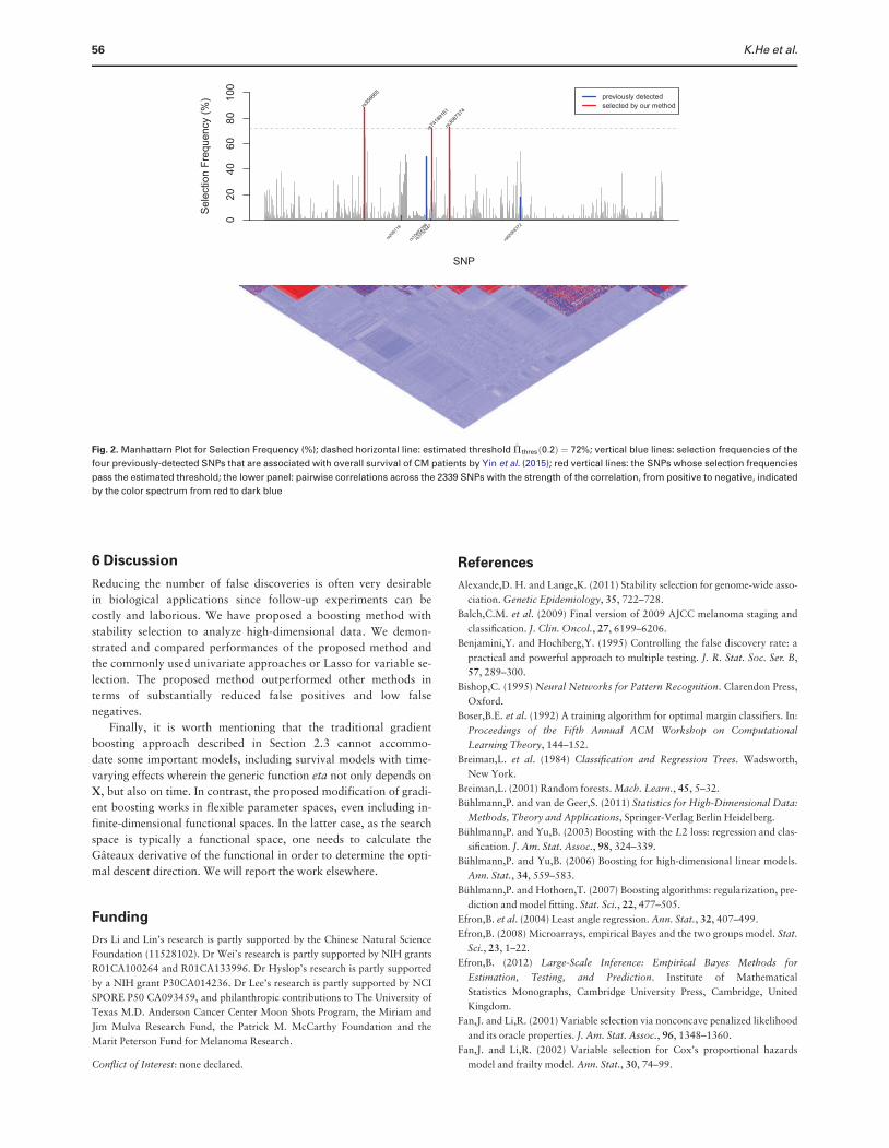
eration is less critical. A Manhattan plot was given in Figure 2 with

the dashed horizontal line corresponding to the estimated threshold

Pthresð0:2Þ ¼ 72%. Three variables have selection frequencies larger

than this dashed horizontal line. The vertical blue lines highlight the

selection frequencies of the four previously-detected SNPs that are

associated with overall survival of CM patients by Yin et al. (2015).

The red vertical lines highlight the SNPs whose selection frequencies

pass the estimated threshold. The lower panel of Figure 2 illustrates

pairwise correlations across the 2339 SNPs with the strength of the

correlation, from positive to negative, indicated by the color spec-

trum from red to dark blue. One of the top SNPs in our finding,

rs74189161 (with selection frequency¼72% and Fdr ¼ 0:16) is

strongly correlated with rs3752447 identified by Yin et al. (2015),

with correlation coefficients r2 ¼ 1 (calculated with plink v1.07;

Purcell et al., 2007). Besides confirming the previously reported

SNP, we also found some novel signals. For example, we identified a

cluster of signals around SNP rs356665 in gene FANCC and a SNP

rs3087374 in gene FANC1. Both two genes have previously been re-

ported having regulation effects with the FA pathway (Thompson

et al., 2012; Jenkins et al., 2012; Kao et al., 2011). Mutations in the

FA pathway are identified in diverse cancer types (Hucl and

Gallmeier, 2011) and therefore are likely to modulate the survival of

CM patients.

Table 3. Summary of selected SNPs by Lasso (sorted by the magni-

tude of coefficients; only predictors with absolute coefficients

larger than 0.01 are included), their estimated coefficients by

boosting without stability selection, P-values based on univariate

approach, selection frequencies based on stability selection

SNPs Chromosome Gene bLasso bBoosting P-value Frequency

(%)

rs74189161 13 BRCA2 �0.11 �0.10 0.002 72*

rs356665 9 FANCC �0.09 �0.04 0.03 88*

rs11649642 16 FANCA �0.08 �0.05 0.01 27

rs9567670 13 BRCA2 �0.07 �0.03 0.01 51

rs8081200 17 BRIP1 �0.06 �0.02 0.05 38

rs3087374 15 FANC1 �0.06 �0.01 0.02 73*

rs35322368 9 FANCC 0.06 0 0.03 65

rs57119673 16 FANCA �0.04 �0.01 0.03 54

rs8061528 16 BTBD12 �0.03 0 0.12 36

rs2247233 15 FANC1 0.02 0 0.15 39

rs848286 2 FANCL 0.02 0 0.02 23

rs62032982 16 PALB2 0.01 0 0.04 34

bLasso: coefficients from Lasso; bBoosting: coefficients from boosting; P-value:

calculated from univariate approach; Frequency ð%Þ: selection frequencies

across 100 subsampling; Fdr: estimated empirical Bayes false discovery rate

(based 500 permuted samples); the false discovery control of the predictors

under stability selection are coded by (*) to indicate that the selection frequen-

cies pass the Fdr threshold.

Table 4. Numbers of selected variables

Lasso Boosting Stability selection

25 7 3

0 100 200 300 400 500

0.0

0.2

0.4

0.6

0.8

1.0

Iteration

Sel

ectio

n F

requ

ency

(%

) Above ThresholdUnder Threshold

Fig. 1. Selection Path: selection frequencies across 500 boosting iterations;

Threshold: estimated empirical Bayes false discovery rate Fdr �0:2 (based

500 permuted samples)

Component-wise gradient boosting and false discovery control 55

6 Discussion

Reducing the number of false discoveries is often very desirable

in biological applications since follow-up experiments can be

costly and laborious. We have proposed a boosting method with

stability selection to analyze high-dimensional data. We demon-

strated and compared performances of the proposed method and

the commonly used univariate approaches or Lasso for variable se-

lection. The proposed method outperformed other methods in

terms of substantially reduced false positives and low false

negatives.

Finally, it is worth mentioning that the traditional gradient

boosting approach described in Section 2.3 cannot accommo-

date some important models, including survival models with time-

varying effects wherein the generic function eta not only depends on

X, but also on time. In contrast, the proposed modification of gradi-

ent boosting works in flexible parameter spaces, even including in-

finite-dimensional functional spaces. In the latter case, as the search

space is typically a functional space, one needs to calculate the

Gateaux derivative of the functional in order to determine the opti-

mal descent direction. We will report the work elsewhere.

Funding

Drs Li and Lin’s research is partly supported by the Chinese Natural Science

Foundation (11528102). Dr Wei’s research is partly supported by NIH grants

R01CA100264 and R01CA133996. Dr Hyslop’s research is partly supported

by a NIH grant P30CA014236. Dr Lee’s research is partly supported by NCI

SPORE P50 CA093459, and philanthropic contributions to The University of

Texas M.D. Anderson Cancer Center Moon Shots Program, the Miriam and

Jim Mulva Research Fund, the Patrick M. McCarthy Foundation and the

Marit Peterson Fund for Melanoma Research.

Conflict of Interest: none declared.

References

Alexande,D. H. and Lange,K. (2011) Stability selection for genome-wide asso-

ciation. Genetic Epidemiology, 35, 722–728.

Balch,C.M. et al. (2009) Final version of 2009 AJCC melanoma staging and

classification. J. Clin. Oncol., 27, 6199–6206.

Benjamini,Y. and Hochberg,Y. (1995) Controlling the false discovery rate: a

practical and powerful approach to multiple testing. J. R. Stat. Soc. Ser. B,

57, 289–300.

Bishop,C. (1995) Neural Networks for Pattern Recognition. Clarendon Press,

Oxford.

Boser,B.E. et al. (1992) A training algorithm for optimal margin classifiers. In:

Proceedings of the Fifth Annual ACM Workshop on Computational

Learning Theory, 144–152.

Breiman,L. et al. (1984) Classification and Regression Trees. Wadsworth,

New York.

Breiman,L. (2001) Random forests. Mach. Learn., 45, 5–32.

Buhlmann,P. and van de Geer,S. (2011) Statistics for High-Dimensional Data:

Methods, Theory and Applications, Springer-Verlag Berlin Heidelberg.

Buhlmann,P. and Yu,B. (2003) Boosting with the L2 loss: regression and clas-

sification. J. Am. Stat. Assoc., 98, 324–339.

Buhlmann,P. and Yu,B. (2006) Boosting for high-dimensional linear models.

Ann. Stat., 34, 559–583.

Buhlmann,P. and Hothorn,T. (2007) Boosting algorithms: regularization, pre-

diction and model fitting. Stat. Sci., 22, 477–505.

Efron,B. et al. (2004) Least angle regression. Ann. Stat., 32, 407–499.

Efron,B. (2008) Microarrays, empirical Bayes and the two groups model. Stat.

Sci., 23, 1–22.

Efron,B. (2012) Large-Scale Inference: Empirical Bayes Methods for

Estimation, Testing, and Prediction. Institute of Mathematical

Statistics Monographs, Cambridge University Press, Cambridge, United

Kingdom.

Fan,J. and Li,R. (2001) Variable selection via nonconcave penalized likelihood

and its oracle properties. J. Am. Stat. Assoc., 96, 1348–1360.

Fan,J. and Li,R. (2002) Variable selection for Cox’s proportional hazards

model and frailty model. Ann. Stat., 30, 74–99.

Fig. 2. Manhattarn Plot for Selection Frequency (%); dashed horizontal line: estimated threshold P thresð0:2Þ ¼ 72%; vertical blue lines: selection frequencies of the

four previously-detected SNPs that are associated with overall survival of CM patients by Yin et al. (2015); red vertical lines: the SNPs whose selection frequencies

pass the estimated threshold; the lower panel: pairwise correlations across the 2339 SNPs with the strength of the correlation, from positive to negative, indicated

by the color spectrum from red to dark blue

56 K.He et al.

Freund,Y. and Schapire,R. (1996) Experiments with a new boosting algo-

rithm. Machine Learning: Proceedings of the Thirteenth International

Conference, Morgan Kauffman, San Francisco, pp. 148–156.

Friedman,J.H. et al. (2000) Additive logistic regression: a statistical view of

boosting (with discussion). Ann. Stat., 28, 337–407.

Friedman,J.H. (2001) Greedy function approximation: a gradient boosting

machine. Ann. Stat., 29, 1189–1232.

Geoman,J.J. (2010) L1 penalized estimation in the Cox proportional hazards

model. Biometrical Journal, 52, 70–84.

Gui,J. and Li,H. (2005) Penalized cox regression analysis in the high-

dimensional and low-sample size settings with application to microarray

gene expression data. Bioinformatics, 21, 3001–3008.

Hastie,T.J. and Tibshirani,R.J. (1990) Generalized Additive Models.

Chapman and Hall/CRC.

Hastie,T. et al. (2009) The Elements of Statistical Learning: Data Mining,

Inference, and Prediction, Springer, New York.

Hucl,T. and Callmeier,E. (2010) DNA repair: exploiting the Fanconi Anemia

Pathway as a potential therapeutic target. Physiol. Res., 60, 453–465.

Hunter,D.R. and Lange,K. (2004) A tutorial on MM algorithms. Am. Stat.,

58, 30–37.

Jenkins,C. et al. (2012) Targeting the Fanconi Anemia Pathway to identify tail-

ored anticancer therapeutics. Anemia, Article ID 481583.

Kao,W.H. et al. (2011) Upregulation of Fanconi anemia DNA repair genes in

melanoma compared with non-melanoma skin cancer. J. Investig.

Dermatol., 131, 2139–2142.

Lange,K. (2013) Optimization. 2nd edn. Springer Texts in Statistics In:

Casella,G. et al (eds), Springer, New York.

Li,H. and Luan,Y. (2005) Boosting proportional hazards models using

smoothing splines, with applications to high-dimensional microarray data.

Bioinformatics, 21, 2403–2409.

Liu,H. et al. (2012) Influence of single nucleotide polymorphisms in the

MMP1 promoter region on cutaneous melanoma progression. Melanoma

Res., 22, 169–75.

Meinshausen,N. and Buhlmann,P. (2010) Stability selection (with discussion).

J. R. Stat. Soc. Ser. B, 72, 417–473.

Purcell,S. et al. (2007) PLINK: a toolset for whole-genome association and

population-based linkage analysis. Am. J. Hum. Genet., 81, 559–575.

Rendleman,J. et al. (2013) Melanoma risk loci as determinants of melanoma recur-

rence and survival. J. Transl. Med., 11, 1–14. doi: 10.1186/1479-5876-11-279.

Ridgeway,G. (1999) The state of boosting. Comput. Sci. Stat., 31, 172–181.

Schramm,S.J. and Mann,G.J. (2011) Melanoma prognosis: a REMARK-

based systematic review and bioinformatic analysis of immunohistochemi-

cal and gene microarray studies. Mol. Cancer Therap., 10, 1520–1528.

Simon,N. et al. (2011) Regularization paths for Cox’s proportional hazards

model via coordinate descent. J. Stat. Softw., 39, 1–13.

Storey,J.D. (2003) The positive false discovery rate: a Bayesian interpretation

and the q-value. Ann. Stat., 31, 2013–2035.

Thompson,E.R. et al. (2012) Exome sequencing identifies rare deleterious

mutations in DNA repair genes FANCC and BLM as potential breast cancer

susceptibility alleles. PLOS Genet., 8, e1002894.

Tibshirani,R. (1996) Regression shrinkage and selection via the lasso. J. R.

Stat. Soc. Ser. B (Methodological), 58, 267–288.

Tibshirani,R. (1997) The lasso method for variable selection in the Cox model.

Stat. Med., 16, 385–395.

Tusher,V.G. et al. (2001) Significance analysis of microarrays applied to the

ionizing radiation response. Proc. Natl. Acad. Sci. USA, 98, 5116–5121.

Yin,J. et al. (2015) Genetic variants in Fanconi Anemia pathway genes BRCA2 and

FANCA predict Melanoma survival. J. Investig. Dermatol. 135, 542–550.

Zhao,D.S. and Li,Y. (2010) Principled sure independence screening for Cox mod-

els with ultra-high-dimensional covariates. manuscript, Harvard University.

Component-wise gradient boosting and false discovery control 57