Complexified Hamiltonian Symplectomorphismsand Solutions of the Homogeneous Complex

Monge–Ampere Equation

Jose Mourao

CAMGSD, Mathematics Department, IST

Hong Kong Geometry Colloquium

December 3, 2016

On work in collaboration with Joao P. Nunes

Index

1. HCMA and imaginary time Hamiltonian flows . . . . . . . . . . . . . . . . . . . . . . 3

2. HCMA and the geometry of the space of Kahler metrics on M . . . . . . 8

3. Explicit “rotation” of hamiltonian flows to imaginary time . . . . . . . . . 15

4. Infinite dimensional spaces of new solutions of the HCMA . . . . . . . . . . 18

4.1. Solutions with Rn-invariant initial data, HRMA and Legendre trans-forms 18

4.2. New solutions of the HCMA on an elliptic curve 22

4.3. New solutions of the HCMA on CP1 24

2

1. HCMA and imaginary time Hamiltonian flows

The Homogeneuous Complex Monge–Ampere (HCMA) equa-

tion is the following nonlinear equation on a complex (n + 1)–

dimensional manifold N

MA(Φ) := det

(∂2Φ

∂zj∂zk

)= 0,

or, equivalently, (∂∂Φ

)n+1= 0. (1)

It is a very difficult equation with very few (genuinly complex)

solutions known.

3

Even for n = 1 it is very nontrivial.For functions Φ on (open subsets of) N = [0, T ]× S1 ×M , which are

(a) S1–invariant and(b) such that g11 = ∂2Φ

∂z∂z(t, z, z) > 0

(i.e. φt = Φ(t, ·) is a path of Kahler potentials on M), we have(∂N ∂N Φ

)2= 0 ⇔

∂2Φ

∂t2∂2Φ

∂z∂z− |

∂2Φ

∂t∂z|2 = 0⇔

∂2Φ

∂t2= g11|

∂2Φ

∂t∂z|2 ⇔

φt = ||∇φt||2φt (2)

4

Ellaborating on an idea of Semmes and Donaldson we will show

how to reduce the Cauchy problem for (2)φt = ||∇φt||2φtφ0 = k,φ0 = H,

k ∈ C∞(U), H ∈ C∞(M). (3)

to the problem of finding the integral curves of the Hamiltonian

vector field XωH, where ω = i∂∂k, followed by “rotating” t to the

imaginary axis (in the complex t–plane)

exp(sXωH) exp(

√−1tXω

H) ∈ HamC(M,ω)??⊂ Diff(M), (4)

in a certain way.

5

To make sense of (4) we must be working on the symplecticpicture (see section 3 below) in which ω is fixed and the complexstructure Jt changes.

Then the imaginary time integral curves in (4) are solutions ofthe following coupled system{

xt = JtXωH = ∇γtH

Jt =(exp(

√−1tXω

H))∗

(J).(5)

Then Donaldson shows that a solution of (3) is given by theKahler potential φt of ωt in

ωt =((

exp(√−1tXω

H))−1

)∗(ω) . (6)

This is the so called Donaldson formal solution of the CHMA.6

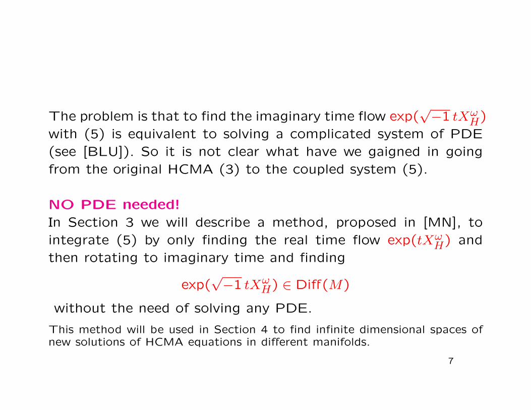
The problem is that to find the imaginary time flow exp(√−1 tXω

H)with (5) is equivalent to solving a complicated system of PDE(see [BLU]). So it is not clear what have we gaigned in goingfrom the original HCMA (3) to the coupled system (5).

NO PDE needed!

In Section 3 we will describe a method, proposed in [MN], tointegrate (5) by only finding the real time flow exp(tXω

H) andthen rotating to imaginary time and finding

exp(√−1 tXω

H) ∈ Diff(M)

without the need of solving any PDE.

This method will be used in Section 4 to find infinite dimensional spaces ofnew solutions of HCMA equations in different manifolds.

7

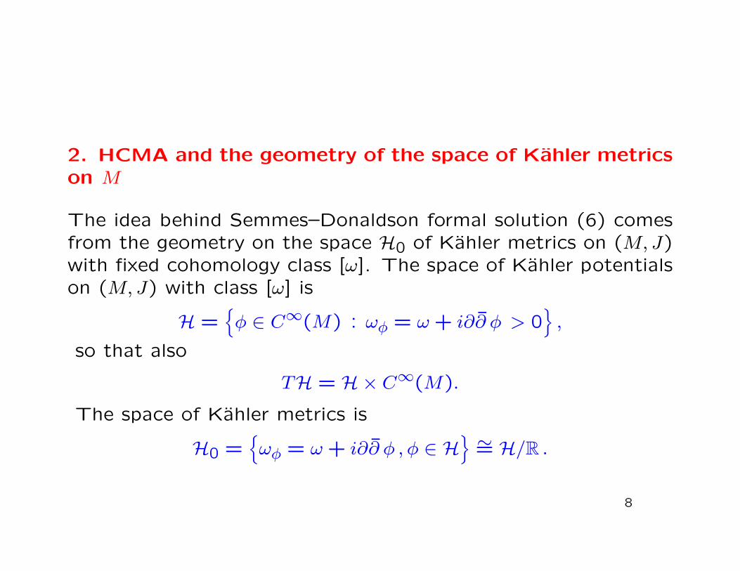
2. HCMA and the geometry of the space of Kahler metricson M

The idea behind Semmes–Donaldson formal solution (6) comesfrom the geometry on the space H0 of Kahler metrics on (M,J)with fixed cohomology class [ω]. The space of Kahler potentialson (M,J) with class [ω] is

H ={φ ∈ C∞(M) : ωφ = ω + i∂∂ φ > 0

},

so that also

TH = H× C∞(M).

The space of Kahler metrics is

H0 ={ωφ = ω + i∂∂ φ , φ ∈ H

} ∼= H/R .8

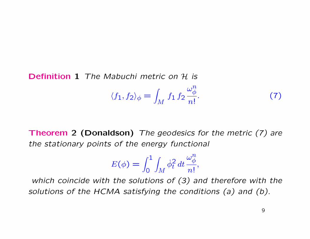
Definition 1 The Mabuchi metric on H is

〈f1, f2〉φ =∫Mf1 f2

ωnφ

n!. (7)

Theorem 2 (Donaldson) The geodesics for the metric (7) are

the stationary points of the energy functional

E(φ) =∫ 1

0

∫Mφ2t dt

ωnφ

n!,

which coincide with the solutions of (3) and therefore with the

solutions of the HCMA satisfying the conditions (a) and (b).

9

Donaldson further shows in [Do1] that H0 with the Mabuchi me-

tric is an infinite dimensional analogue of the symmetric spaces

of non–compact type of the form

PSL(N,C)/PSU(N) ,

with PSL(N,C)–invariant metric.

10

1. H0 as a quotient

Let

HamC(M,ω) :={ϕ ∈ Diff(M) :

(ϕ−1

)∗(ω) ∈ H0

} no subgroup⊂ Diff(M),

(8)

we obtain, from Moser theorem,

HamC(M,ω)/Ham(M,ω) ∼= H0

ϕ 7→(ϕ−1

)∗(ω) .

2. TωH0∼= C∞(M)/R

We have

LJX

ωφH

(ωφ)

= i∂∂H,

11

3. Curvature formulas

Theorem 3 (Donaldson) The curvature of the Mabuchi metric

(7) and the sectional curvature read

Rφ(f1, f2)f3 = −1

4{{f1, f2}φ, f3}φ, Kφ(f1, f2) = −

1

4||{f1, f2}φ||2φ .

for all f1, f2, f3 ∈ TφH0, where

TφH0 ={f ∈ C∞(M) :

∫Mfωφ

n!= 0

}∼= Lie(Ham(M,ωφ)) .

12

The above expressions are in full agreement with the formulas for

the curvature of the finite dimensional symmetric spaces KC/K,

R(X,Y )Z = −1

4[[X,Y ], Z]

and

K(X,Y ) = −1

4||[X,Y ]||2 .

for all X,Y, Z ∈ T0KC/K∼= iLie(K) ∼= Lie(K) and the Lie brac-

kets are calculated in Lie(K).

13

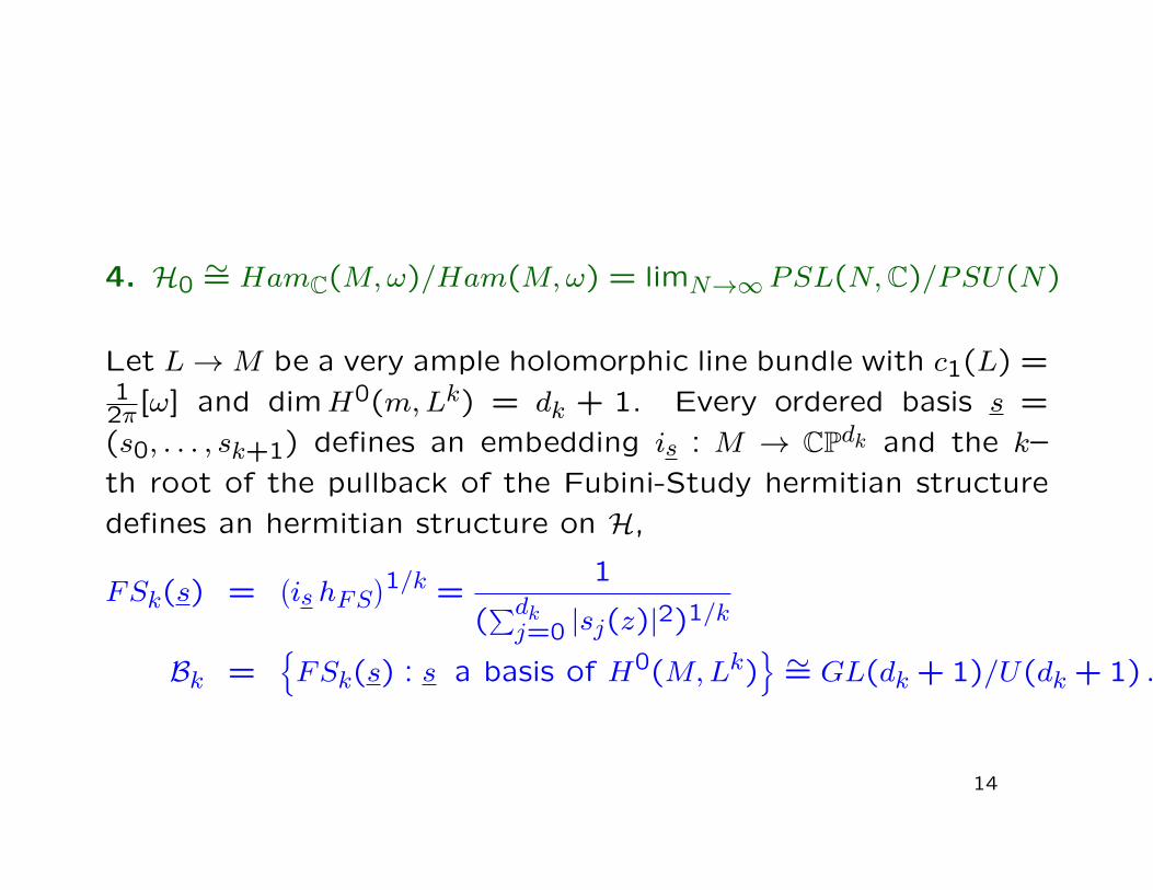
4. H0∼= HamC(M,ω)/Ham(M,ω) = limN→∞ PSL(N,C)/PSU(N)

Let L→M be a very ample holomorphic line bundle with c1(L) =1

2π[ω] and dimH0(m,Lk) = dk + 1. Every ordered basis s =

(s0, . . . , sk+1) defines an embedding is : M → CPdk and the k–

th root of the pullback of the Fubini-Study hermitian structure

defines an hermitian structure on H,

FSk(s) =(is hFS

)1/k =1

(∑dkj=0 |sj(z)|2)1/k

Bk ={FSk(s) : s a basis of H0(M,Lk)

} ∼= GL(dk + 1)/U(dk + 1) .

14

Every h ∈ H defines an inner product on H0(M,Lk)

〈s, s〉k =∫M

(s, s)hkωmhm!

Let s(k) be an orthonormal basis for 〈·, ·〉k and let

h(k) = FSk(s(k)) ∈ Bk

Theorem 4 (Tian, 1990)

h = limk→∞

h(k) .

15

3. Explicit “rotation”of hamiltonian flows to imaginary

time

The missing step to transform Donaldson formal solution of the

Cauchy problem (3) for the HCMA given by (6) into an actual

solution is the rotation (4)

exp(sXωH) exp(

√−1tXω

H).

In the present section we will describe our solution to this pro-

blem obtained in [M-Nunes, IMNR2015]. One key technical tool

to rotate the flow is the Grobner theory of Lie series of vec-

tor fields (which is still very popular in numerical methods in

astronomy – satelite motion, exoplanets, etc).

16

Theorem 5 Let (M,J) be a compact complex manifold and X ∈X (M) an analytic vector field. There exist local charts ((zj), U)in neighourhoods of every point and T > 0 such that for allτ ∈ DT the functions

zτj = eτX zj = uτj (x, y) +√−1vτj (x, y), (9)

where xj = <(zj), yj = =(zj), uτj (x, y) = <(zτj ), vτj (x, y) = =(zτj ),

define on V ⊂ U local Jτ–holomorphic charts for a unique com-plex structure Jτ and there exists a unique diffeomorphism ϕ

X,Jτ

such that (ϕX,Jτ

)∗J = Jτ .

The complex time flow is then given explicitly locally by

ϕX,Jτ (x, y) = (uτ(x, y), vτ(x, y)), (10)

17

We see that, as expected, if τ = t ∈ R the complex time flow is

J–independent and coincides with the real time flow

ϕX,Jt = ϕXt .

Theorem 6 (M-Nunes) Consider the Cauchy problem for the

HCMA (3) on I×M (where we are already supressing the angular

coordinate of the first factor in A × M). Then by replacing

exp(√−1tXω

H), in the formal solution (6), by ϕXH ,Jit obtained as

in (10) one obtains a solution of (3).

18

4. Infinite dimensional spaces of new solutions of the

HCMA

4.1 Solutions with Rn-invariant initial data, HRMA and Le-

gendre transforms

Suppose that one can choose holomorphic charts with coordina-

tes zj = xj + iyj such that the initial data in (3) do not depend

on y

φ0(x, y) = k(x, y) = k(x)

φ0(x, y) = H(x, y) = H(x).

19

Particular cases of this situation are toric Kahler metrics on to-

ric manifolds with also torus–invariant initial velocities φ0 = H.

Then the HCMA becomes the HRMA equation

detn+1Hessx(Φ) = 0,

where x = (t, x).

20

It is well known that the geodesic equation (3) in this case is linearized bythe Legendre transform associated with φ

φ 7→ g = L(φ)

uj =∂φ

∂xj

g(u) =∑j

xj(u)uj − φ(x(u))

because in the space of the symplectic potentials g the geodesic equationbecomes

gt = 0,

and therefore the solutions are straight lines

gt = L(k) + tH,

where H(u) = H(x(u)).

21

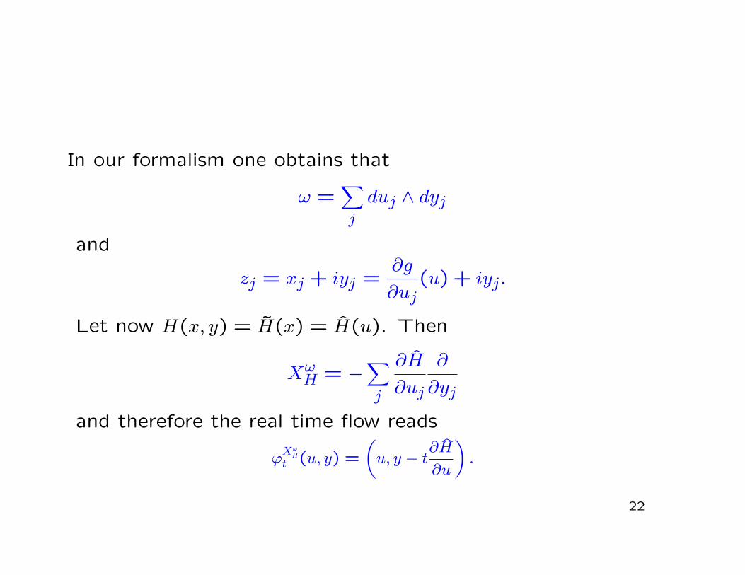
In our formalism one obtains that

ω =∑j

duj ∧ dyj

and

zj = xj + iyj =∂g

∂uj(u) + iyj.

Let now H(x, y) = H(x) = H(u). Then

XωH = −

∑j

∂H

∂uj

∂

∂yj

and therefore the real time flow reads

ϕXω

H

t (u, y) =

(u, y − t

∂H

∂u

).

22

Then, as in (9), to find the rotation of the flow to the imaginary

axis we have to act with the real time flow on J–holomorphic

coordinates and analytically continue t only for those functions.

We have

zitj = exp(itXωH)(zj) =

∂g

∂u+ i

(y − it

∂H

∂u

)=

∂

∂u

(g + tH

)+ iy.

Comparing with (10) we see that indeed gt varies (affine) linearly

with t and the rotation of the real time flow to the imaginary

axis is the composition of two Legendre transforms

ϕXωH

it (x, y) = (Lg+tH ◦ Lk(x), y).

23

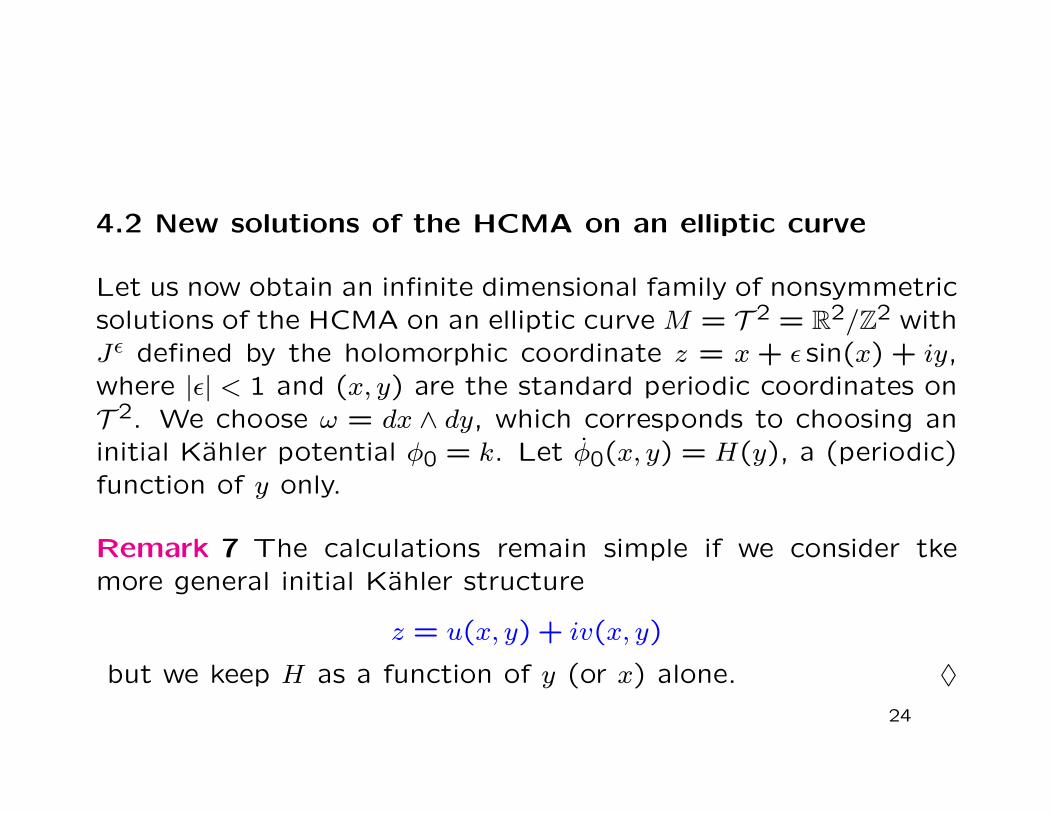
4.2 New solutions of the HCMA on an elliptic curve

Let us now obtain an infinite dimensional family of nonsymmetricsolutions of the HCMA on an elliptic curve M = T 2 = R2/Z2 withJε defined by the holomorphic coordinate z = x + ε sin(x) + iy,where |ε| < 1 and (x, y) are the standard periodic coordinates onT 2. We choose ω = dx ∧ dy, which corresponds to choosing aninitial Kahler potential φ0 = k. Let φ0(x, y) = H(y), a (periodic)function of y only.

Remark 7 The calculations remain simple if we consider tkemore general initial Kahler structure

z = u(x, y) + iv(x, y)

but we keep H as a function of y (or x) alone. ♦

24

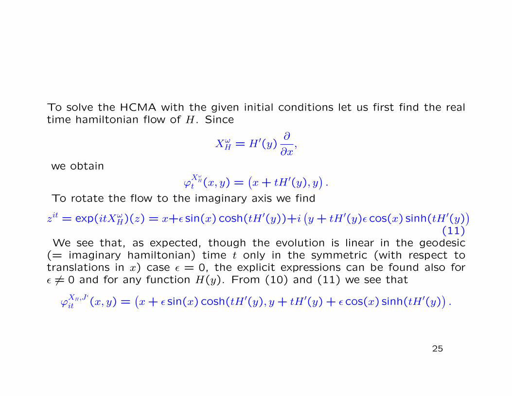
To solve the HCMA with the given initial conditions let us first find the realtime hamiltonian flow of H. Since

XωH = H ′(y)

∂

∂x,

we obtain

ϕXω

H

t (x, y) =(x+ tH ′(y), y

).

To rotate the flow to the imaginary axis we find

zit = exp(itXωH)(z) = x+ε sin(x) cosh(tH ′(y))+i

(y + tH ′(y)ε cos(x) sinh(tH ′(y)

)(11)

We see that, as expected, though the evolution is linear in the geodesic(= imaginary hamiltonian) time t only in the symmetric (with respect totranslations in x) case ε = 0, the explicit expressions can be found also forε 6= 0 and for any function H(y). From (10) and (11) we see that

ϕXH,J ε

it (x, y) =(x+ ε sin(x) cosh(tH ′(y), y + tH ′(y) + ε cos(x) sinh(tH ′(y)

).

25

4.3 New solutions of the HCMA on CP1

26

Thank you!

27