CANNAS DA SILVA, A., Introduction to Symplectic and Hamiltonian Geometry, 2002.pdf
Chapter VI.Symplectic Integration of HamiltonianSystems
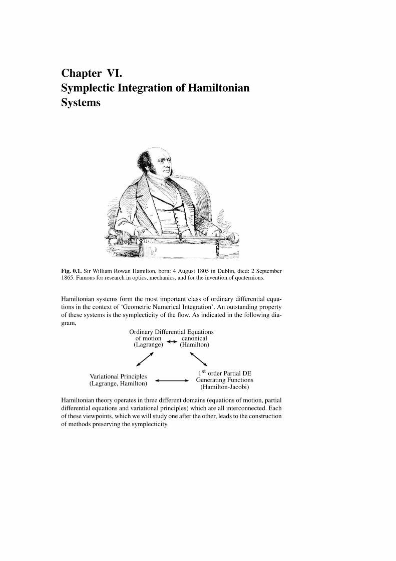
Fig. 0.1. Sir William Rowan Hamilton, born: 4 August 1805 in Dublin, died: 2 September1865. Famous for research in optics, mechanics, and for the invention of quaternions.
Hamiltonian systems form the most important class of ordinary differential equa-tions in the context of ‘Geometric Numerical Integration’. An outstanding propertyof these systems is the symplecticity of the flow. As indicated in the following dia-gram,
Ordinary Differential Equationsof motion canonical
(Lagrange) (Hamilton)
1st order Partial DEGenerating Functions
(Hamilton-Jacobi)
Variational Principles(Lagrange, Hamilton)
Hamiltonian theory operates in three different domains (equations of motion, partialdifferential equations and variational principles) which are all interconnected. Eachof these viewpoints, which we will study one after the other, leads to the constructionof methods preserving the symplecticity.
180 VI. Symplectic Integration of Hamiltonian Systems
VI.1 Hamiltonian SystemsHamilton’s equations appeared first, among thousands of other formulas, and in-spired by previous research in optics, in Hamilton (1834). Their importance was im-mediately recognized by Jacobi, who stressed and extended the fundamental ideas,so that, a couple of years later, all the long history of research of Galilei, Newton,Euler and Lagrange, was, in the words of Jacobi (1842), “to be considered as anintroduction”. The next mile-stones in the exposition of the theory were the monu-mental three volumes of Poincare (1892,1893,1899) on celestial mechanics, Siegel’s“Lectures on Celestial Mechanics” (1956), English enlarged edition by Siegel &Moser (1971), and the influential book of V.I. Arnold (1989; first Russian edition1974). Beyond that, Hamiltonian systems became fundamental in many branches ofphysics. One such area, the dynamics of particle accelerators, actually motivated theconstruction of the first symplectic integrators (Ruth 1983).
VI.1.1 Lagrange’s Equations
Equations differentielles pour la solution de tous les problemes de Dy-namique. (J.-L. Lagrange 1788)
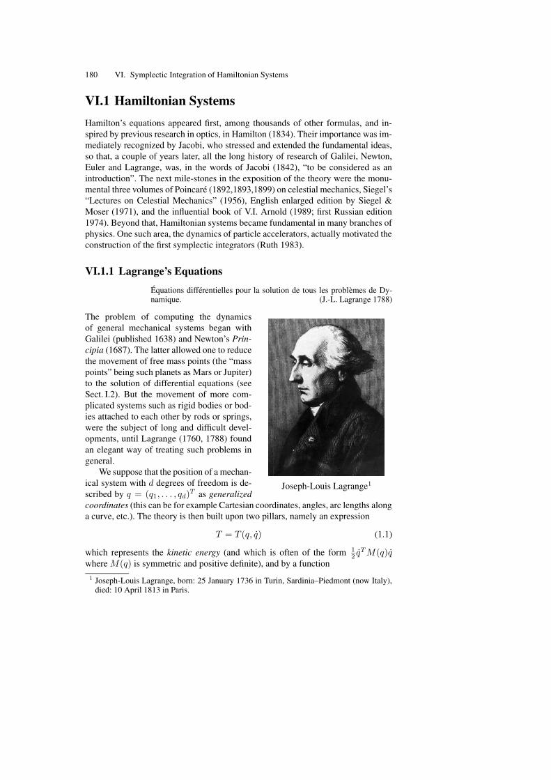
Joseph-Louis Lagrange1
The problem of computing the dynamicsof general mechanical systems began withGalilei (published 1638) and Newton’s Prin-cipia (1687). The latter allowed one to reducethe movement of free mass points (the “masspoints” being such planets as Mars or Jupiter)to the solution of differential equations (seeSect. I.2). But the movement of more com-plicated systems such as rigid bodies or bod-ies attached to each other by rods or springs,were the subject of long and difficult devel-opments, until Lagrange (1760, 1788) foundan elegant way of treating such problems ingeneral.
We suppose that the position of a mechan-ical system with d degrees of freedom is de-scribed by q = (q1, . . . , qd)
T as generalizedcoordinates (this can be for example Cartesian coordinates, angles, arc lengths alonga curve, etc.). The theory is then built upon two pillars, namely an expression
T = T (q, q) (1.1)
which represents the kinetic energy (and which is often of the form 12 q
TM(q)qwhere M(q) is symmetric and positive definite), and by a function1 Joseph-Louis Lagrange, born: 25 January 1736 in Turin, Sardinia–Piedmont (now Italy),
died: 10 April 1813 in Paris.
VI.1 Hamiltonian Systems 181
U = U(q) (1.2)
representing the potential energy. Then, after denoting by
L = T − U (1.3)
the corresponding Lagrangian, the coordinates q1(t), . . . , qd(t) obey the differentialequations
d
dt
(∂L
∂q
)=∂L
∂q, (1.4)
which constitute the Lagrange equations of the system. A numerical (or analytical)integration of these equations allows one to predict the motion of any such systemfrom given initial values (“Ce sont ces equations qui serviront a determiner la courbedecrite par le corps M et sa vitesse a chaque instant”; Lagrange 1760, p. 369).
Example 1.1. For a mass point of mass m in R3 with Cartesian coordinates x =
(x1, x2, x3)T we have T (x) = m(x2
1 + x22 + x2
3)/2. We suppose the point to movein a conservative force field F (x) = −∇U(x). Then, the Lagrange equations (1.4)become mx = F (x), which is Newton’s second law. The equations (I.2.2) for theplanetary motion are precisely of this form.
Example 1.2 (Pendulum). For the mathematical pendulum of Sect. I.1 we take theangle α as coordinate. The kinetic and potential energies are given by T = m(x2 +y2)/2 = m`2α2/2 and U = mgy = −mg` cosα, respectively, so that the Lagrangeequations become −mg` sinα−m`2α = 0 or equivalently α+ g
` sinα = 0.
VI.1.2 Hamilton’s Canonical EquationsAn diese Hamiltonsche Form der Differentialgleichungen werden dieferneren Untersuchungen, welche den Kern dieser Vorlesung bilden,anknupfen; das Bisherige ist als Einleitung dazu anzusehen.
(C.G.J. Jacobi 1842, p. 143)
Hamilton (1834) simplified the structure of Lagrange’s equations and turned theminto a form that has remarkable symmetry, by
• introducing Poisson’s variables, the conjugate momenta
pk =∂L
∂qk(q, q) for k = 1, . . . , d, (1.5)
• considering the Hamiltonian
H := pT q − L(q, q) (1.6)
as a function of p and q, i.e., taking H = H(p, q) obtained by expressing q as afunction of p and q via (1.5).
Here it is, of course, required that (1.5) defines, for every q, a continuously differ-entiable bijection q ↔ p. This map is called the Legendre transform.
182 VI. Symplectic Integration of Hamiltonian Systems
Theorem 1.3. Lagrange’s equations (1.4) are equivalent to Hamilton’s equations
pk = −∂H∂qk
(p, q), qk =∂H
∂pk(p, q), k = 1, . . . , d. (1.7)
Proof. The definitions (1.5) and (1.6) for the momenta p and for the Hamiltonian Himply that
∂H
∂p= qT + pT ∂q
∂p− ∂L
∂q
∂q
∂p= qT ,
∂H
∂q= pT ∂q
∂q− ∂L
∂q− ∂L
∂q
∂q
∂q= −∂L
∂q.
The Lagrange equations (1.4) are therefore equivalent to (1.7). ut
Case of Quadratic T . In the case that T = 12 q
TM(q)q is quadratic, where M(q)is a symmetric and positive definite matrix, we have, for a fixed q, p = M(q)q, sothat the existence of the Legendre transform is established. Further, by replacing thevariable q by M(q)−1p in the definition (1.6) of H(p, q), we obtain
H(p, q) = pTM(q)−1p− L(q,M(q)−1p
)
= pTM(q)−1p− 1
2pTM(q)−1p+ U(q) =
1
2pTM(q)−1p+ U(q)
and the Hamiltonian is H = T + U , which is the total energy of the mechanicalsystem.
In Chap. I we have seen several examples of Hamiltonian systems, e.g., the pen-dulum (I.1.13), the Kepler problem (I.2.2), the outer solar system (I.2.12), etc. In thefollowing we consider Hamiltonian systems (1.7) where the Hamiltonian H(p, q) isarbitrary, and so not necessarily related to a mechanical problem.
VI.2 Symplectic TransformationsThe name “complex group” formerly advocated by me in allusion to linecomplexes, . . . has become more and more embarrassing through colli-sion with the word “complex” in the connotation of complex number. Itherefore propose to replace it by the Greek adjective “symplectic.”
(H. Weyl (1939), p. 165)
A first property of Hamiltonian systems, already seen in Example 1.2 of Sect. IV.1,is that the Hamiltonian H(p, q) is a first integral of the system (1.7). In this sectionwe shall study another important property – the symplecticity of its flow. The basicobjects to be studied are two-dimensional parallelograms lying in R
2d. We supposethe parallelogram to be spanned by two vectors
ξ =
(ξp
ξq
), η =
(ηp
ηq
)
in the (p, q) space (ξp, ξq, ηp, ηq are in Rd) as
VI.2 Symplectic Transformations 183
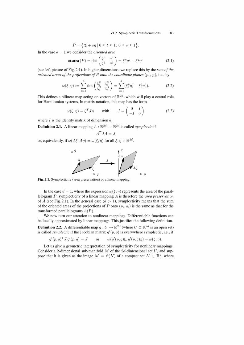
P =tξ + sη | 0 ≤ t ≤ 1, 0 ≤ s ≤ 1
.
In the case d = 1 we consider the oriented area
or.area (P ) = det
(ξp ηp
ξq ηq
)= ξpηq − ξqηp (2.1)
(see left picture of Fig. 2.1). In higher dimensions, we replace this by the sum of theoriented areas of the projections of P onto the coordinate planes (pi, qi), i.e., by
ω(ξ, η) :=d∑
i=1
det
(ξpi ηp
i
ξqi ηq
i
)=
d∑
i=1
(ξpi η
qi − ξq
i ηpi ). (2.2)
This defines a bilinear map acting on vectors of R2d, which will play a central role
for Hamiltonian systems. In matrix notation, this map has the form
ω(ξ, η) = ξTJη with J =
(0 I−I 0
)(2.3)
where I is the identity matrix of dimension d.
Definition 2.1. A linear mapping A : R2d → R
2d is called symplectic if
ATJA = J
or, equivalently, if ω(Aξ,Aη) = ω(ξ, η) for all ξ, η ∈ R2d.
p
q
ξ
η
p
q
Aξ
Aη
A
Fig. 2.1. Symplecticity (area preservation) of a linear mapping.
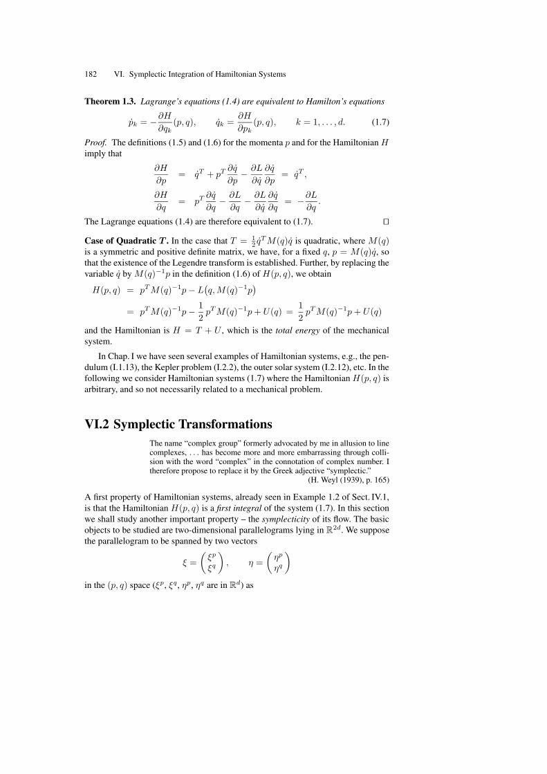
In the case d = 1, where the expression ω(ξ, η) represents the area of the paral-lelogram P , symplecticity of a linear mapping A is therefore the area preservationof A (see Fig. 2.1). In the general case (d > 1), symplecticity means that the sumof the oriented areas of the projections of P onto (pi, qi) is the same as that for thetransformed parallelograms A(P ).
We now turn our attention to nonlinear mappings. Differentiable functions canbe locally approximated by linear mappings. This justifies the following definition.
Definition 2.2. A differentiable map g : U → R2d (where U ⊂ R
2d is an open set)is called symplectic if the Jacobian matrix g′(p, q) is everywhere symplectic, i.e., if
g′(p, q)TJ g′(p, q) = J or ω(g′(p, q)ξ, g′(p, q)η) = ω(ξ, η).
Let us give a geometric interpretation of symplecticity for nonlinear mappings.Consider a 2-dimensional sub-manifold M of the 2d-dimensional set U , and sup-pose that it is given as the image M = ψ(K) of a compact set K ⊂ R
2, where
184 VI. Symplectic Integration of Hamiltonian Systems
ψ(s, t) is a continuously differentiable function. The manifold M can then be con-sidered as the limit of a union of small parallelograms spanned by the vectors
∂ψ
∂s(s, t) ds and
∂ψ
∂t(s, t) dt.
For one such parallelogram we consider (as above) the sum over the oriented areasof its projections onto the (pi, qi) plane. We then sum over all parallelograms of themanifold. In the limit this gives the expression
Ω(M) =
∫∫
K
ω
(∂ψ
∂s(s, t),
∂ψ
∂t(s, t)
)ds dt. (2.4)
The transformation formula for double integrals implies that Ω(M) is independentof the parametrization ψ of M .
Lemma 2.3. If the mapping g : U → R2d is symplectic on U , then it preserves the
expression Ω(M), i.e.,Ω(g(M)
)= Ω(M)
holds for all 2-dimensional manifolds M that can be represented as the image of acontinuously differentiable function ψ.
Proof. The manifold g(M) can be parametrized by g ψ. We have
Ω(g(M)
)=
∫∫
K
ω
(∂(g ψ)
∂s(s, t),
∂(g ψ)
∂t(s, t)
)ds dt = Ω(M),
because (g ψ)′(s, t) = g′(ψ(s, t)
)ψ′(s, t) and g is a symplectic transformation. ut
For d = 1, M is already a subset of R2 and we choose K = M with ψ the
identity map. In this case, Ω(M) =∫∫
Mds dt represents the area of M . Hence,
Lemma 2.3 states that all symplectic mappings (also nonlinear ones) are area pre-serving.
We are now able to prove the main result of this section. We use the notationy = (p, q), and we write the Hamiltonian system (1.7) in the form
y = J−1∇H(y), (2.5)
where J is the matrix of (2.3) and ∇H(y) = H ′(y)T .Recall that the flow ϕt : U → R
2d of a Hamiltonian system is the mapping thatadvances the solution by time t, i.e., ϕt(p0, q0) = (p(t, p0, q0), q(t, p0, q0)), wherep(t, p0, q0), q(t, p0, q0) is the solution of the system corresponding to initial valuesp(0) = p0, q(0) = q0.
Theorem 2.4 (Poincare 1899). Let H(p, q) be a twice continuously differentiablefunction on U ⊂ R
2d. Then, for each fixed t, the flow ϕt is a symplectic transforma-tion wherever it is defined.
Proof. The derivative ∂ϕt/∂y0 (with y0 = (p0, q0)) is a solution of the vari-ational equation which, for the Hamiltonian system (2.5), is of the form Ψ =J−1∇2H
(ϕt(y0)
)Ψ , where∇2H(p, q) is the Hessian matrix ofH(p, q) (∇2H(p, q)
VI.2 Symplectic Transformations 185
−1 0 1 2 3 4 5 6 7 8 9
−2
−1
1
2
A
ϕπ/2(A)
ϕπ(A)
B
ϕπ/2(B)
ϕπ(B)
ϕ3π/2(B)
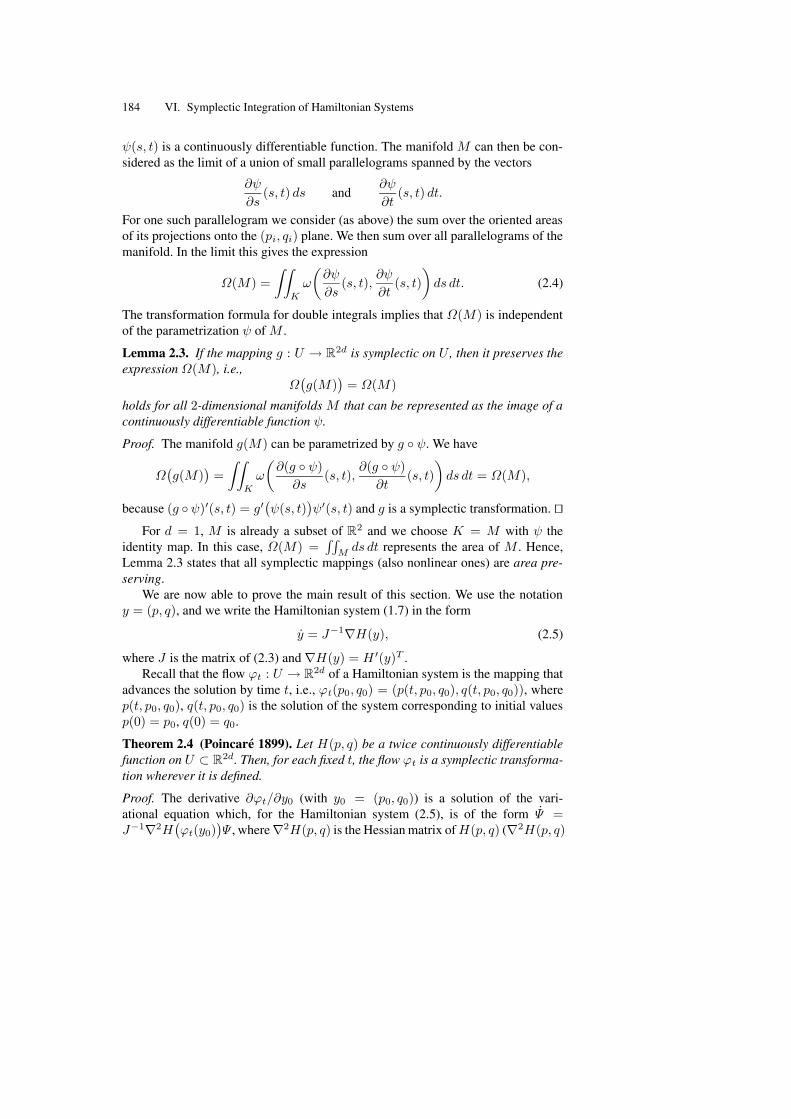
Fig. 2.2. Area preservation of the flow of Hamiltonian systems
is symmetric). We therefore obtain
d
dt
((∂ϕt
∂y0
)T
J(∂ϕt
∂y0
))=( ddt
∂ϕt
∂y0
)T
J(∂ϕt
∂y0
)+(∂ϕt
∂y0
)T
J( ddt
∂ϕt
∂y0
)
=(∂ϕt
∂y0
)T
∇2H(ϕt(y0)
)J−TJ
(∂ϕt
∂y0
)+(∂ϕt
∂y0
)T
∇2H(ϕt(y0)
)(∂ϕt
∂y0
)= 0,
because JT = −J and J−TJ = −I . Since the relation(∂ϕt
∂y0
)T
J(∂ϕt
∂y0
)= J (2.6)
is satisfied for t = 0 (ϕ0 is the identity map), it is satisfied for all t and all (p0, q0),as long as the solution remains in the domain of definition of H . utExample 2.5. We illustrate this theorem with the pendulum problem (Example 1.2)using the normalization m = ` = g = 1. We have q = α, p = α, and the Hamilto-nian is given by
H(p, q) = p2/2 − cos q.
Fig. 2.2 shows level curves of this function, and it also illustrates the area preser-vation of the flow ϕt. Indeed, by Theorem 2.4 and Lemma 2.3, the areas of A andϕt(A) as well as those of B and ϕt(B) are the same, although their appearance iscompletely different.
We next show that symplecticity of the flow is a characteristic property forHamiltonian systems. We call a differential equation y = f(y) locally Hamilto-nian, if for every y0 ∈ U there exists a neighbourhood where f(y) = J−1∇H(y)for some function H .
Theorem 2.6. Let f : U → R2d be continuously differentiable. Then, y = f(y) is
locally Hamiltonian if and only if its flow ϕt(y) is symplectic for all y ∈ U and forall sufficiently small t.
186 VI. Symplectic Integration of Hamiltonian Systems
Proof. The necessity follows from Theorem 2.4. We therefore assume that the flowϕt is symplectic, and we have to prove the local existence of a function H(y) suchthat f(y) = J−1∇H(y). Differentiating (2.6) and using the fact that ∂ϕt/∂y0 is asolution of the variational equation Ψ = f ′
(ϕt(y0)
)Ψ , we obtain
d
dt
((∂ϕt
∂y0
)T
J(∂ϕt
∂y0
))=(∂ϕt
∂y0
)(f ′(ϕt(y0)
)TJ+Jf ′
(ϕt(y0)
))(∂ϕt
∂y0
)= 0.
Putting t = 0, it follows from J = −JT that Jf ′(y0) is a symmetric matrix forall y0. The Integrability Lemma 2.7 below shows that Jf(y) can be written as thegradient of a function H(y). ut
The following integrability condition for the existence of a potential was alreadyknown to Euler and Lagrange (see e.g., Euler’s Opera Omnia, vol. 19. p. 2-3, orLagrange (1760), p. 375).
Lemma 2.7 (Integrability Lemma). Let D ⊂ Rn be open and f : D → R
n becontinuously differentiable, and assume that the Jacobian f ′(y) is symmetric for ally ∈ D. Then, for every y0 ∈ D there exists a neighbourhood and a function H(y)such that
f(y) = ∇H(y) (2.7)
on this neighbourhood. In other words, the differential form f1(y) dy1 + . . . +fn(y) dyn = dH is a total differential.
Proof. Assume y0 = 0, and consider a ball around y0 which is contained in D. Onthis ball we define
H(y) =
∫ 1
0
yT f(ty) dt+ Const .
Differentiation with respect to yk, and using the symmetry assumption ∂fi/∂yk =∂fk/∂yi yields
∂H
∂yk(y) =
∫ 1
0
(fk(ty) + yT ∂f
∂yk(ty)t
)dt =
∫ 1
0
d
dt
(tfk(ty)
)dt = fk(y),
which proves the statement. ut
For D = R2d or for star-shaped regions D, the above proof shows that the func-
tion H of Lemma 2.7 is globally defined. Hence the Hamiltonian of Theorem 2.6is also globally defined in this case. This remains valid for simply connected setsD. A counter-example, which shows that the existence of a global Hamiltonian inTheorem 2.6 is not true for general D, is given in Exercise 6.
An important property of symplectic transformations, which goes back to Jacobi(1836, “Theorem X”), is that they preserve the Hamiltonian character of the differ-ential equation. Such transformations have been termed canonical since the 19thcentury. The next theorem shows that canonical and symplectic transformations arethe same.
VI.3 First Examples of Symplectic Integrators 187
Theorem 2.8. Let ψ : U → V be a change of coordinates such that ψ and ψ−1
are continuously differentiable functions. If ψ is symplectic, the Hamiltonian systemy = J−1∇H(y) becomes in the new variables z = ψ(y)
z = J−1∇K(z) with K(z) = H(y). (2.8)
Conversely, if ψ transforms every Hamiltonian system to another Hamiltonian sys-tem via (2.8), then ψ is symplectic.
Proof. Since z = ψ′(y)y and ψ′(y)T∇K(z) = ∇H(y), the Hamiltonian systemy = J−1∇H(y) becomes
z = ψ′(y)J−1ψ′(y)T∇K(z) (2.9)
in the new variables. It is equivalent to (2.8) if
ψ′(y)J−1ψ′(y)T = J−1. (2.10)
Multiplying this relation from the right by ψ′(y)−T and from the left by ψ′(y)−1
and then taking its inverse yields J = ψ′(y)TJψ′(y), which shows that (2.10) isequivalent to the symplecticity of ψ.
For the inverse relation we note that (2.9) is Hamiltonian for all K(z) if andonly if (2.10) holds. ut
VI.3 First Examples of Symplectic Integrators
Feng Kang2
Since symplecticity is a characteristic prop-erty of Hamiltonian systems (Theorem 2.6),it is natural to search for numerical methodsthat share this property. Pioneering work onsymplectic integration is due to de Vogelaere(1956), Ruth (1983), and Feng Kang (1985).Books on the now well-developed subject areSanz-Serna & Calvo (1994) and Leimkuhler& Reich (2004).
Definition 3.1. A numerical one-step methodis called symplectic if the one-step map
y1 = Φh(y0)
is symplectic whenever the method is appliedto a smooth Hamiltonian system.2 Feng Kang, born: 9 September 1920 in Nanjing (China), died: 17 August 1993 in Beijing;
picture obtained from Yuming Shi with the help of Yifa Tang.
188 VI. Symplectic Integration of Hamiltonian Systems
0 2 4 6 8
−2
2
0 2 4 6 8
−2
2
0 2 4 6 8
−2
2
0 2 4 6 8
−2
2
0 2 4 6 8
−2
2
0 2 4 6 8
−2
2
0 2 4 6 8
−2
2
0 2 4 6 8
−2
2
0 2 4 6 8
−2
2
0 2 4 6 8
−2
2
0 2 4 6 8
−2
2
0 2 4 6 8
−2
2
explicit Euler Runge, order 2
symplectic Euler Verlet
implicit Euler midpoint rule
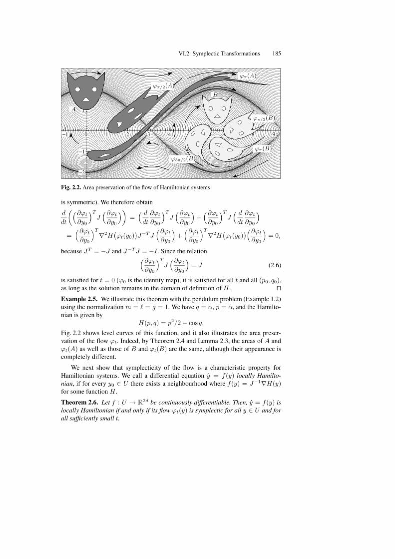
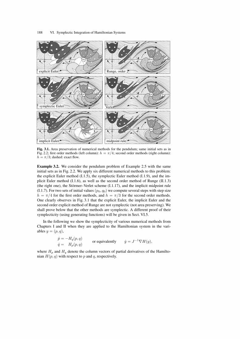
Fig. 3.1. Area preservation of numerical methods for the pendulum; same initial sets as inFig. 2.2; first order methods (left column): h = π/4; second order methods (right column):h = π/3; dashed: exact flow.
Example 3.2. We consider the pendulum problem of Example 2.5 with the sameinitial sets as in Fig. 2.2. We apply six different numerical methods to this problem:the explicit Euler method (I.1.5), the symplectic Euler method (I.1.9), and the im-plicit Euler method (I.1.6), as well as the second order method of Runge (II.1.3)(the right one), the Stormer–Verlet scheme (I.1.17), and the implicit midpoint rule(I.1.7). For two sets of initial values (p0, q0) we compute several steps with step sizeh = π/4 for the first order methods, and h = π/3 for the second order methods.One clearly observes in Fig. 3.1 that the explicit Euler, the implicit Euler and thesecond order explicit method of Runge are not symplectic (not area preserving). Weshall prove below that the other methods are symplectic. A different proof of theirsymplecticity (using generating functions) will be given in Sect. VI.5.
In the following we show the symplecticity of various numerical methods fromChapters I and II when they are applied to the Hamiltonian system in the vari-ables y = (p, q),
p = −Hq(p, q)
q = Hp(p, q)or equivalently y = J−1∇H(y),
where Hp and Hq denote the column vectors of partial derivatives of the Hamilto-nian H(p, q) with respect to p and q, respectively.
VI.3 First Examples of Symplectic Integrators 189
Theorem 3.3 (de Vogelaere 1956). The so-called symplectic Euler methods (I.1.9)
pn+1 = pn − hHq(pn+1, qn)
qn+1 = qn + hHp(pn+1, qn)or
pn+1 = pn − hHq(pn, qn+1)
qn+1 = qn + hHp(pn, qn+1)(3.1)
are symplectic methods of order 1.
Proof. We consider only the method to the left of (3.1). Differentiation with respectto (pn, qn) yields
(I + hHT
qp 0−hHpp I
)(∂(pn+1, qn+1)
∂(pn, qn)
)=
(I −hHqq
0 I + hHqp
),
where the matricesHqp, Hpp, . . . of partial derivatives are all evaluated at (pn+1, qn).This relation allows us to compute ∂(pn+1,qn+1)
∂(pn,qn) and to check in a straightforward
way the symplecticity condition(∂(pn+1,qn+1)
∂(pn,qn)
)TJ(∂(pn+1,qn+1)
∂(pn,qn)
)= J . ut
The methods (3.1) are implicit for general Hamiltonian systems. For separableH(p, q) = T (p) + U(q), however, both variants turn out to be explicit. It is inter-esting to mention that there are more general situations where the symplectic Eulermethods are explicit. If, for a suitable ordering of the components,
∂H
∂qi(p, q) does not depend on pj for j ≥ i, (3.2)
then the left method of (3.1) is explicit, and the components of pn+1 can be com-puted one after the other. If, for a possibly different ordering of the components,
∂H
∂pi(p, q) does not depend on qj for j ≥ i, (3.3)
then the right method of (3.1) is explicit. As an example consider the Hamiltonian
H(pr, pϕ, r, ϕ) =1
2
(p2
r + r−2p2ϕ
)− r cosϕ+ (r − 1)2,
which models a spring pendulum in polar coordinates. For the ordering ϕ < r,condition (3.2) is fulfilled, and for the inverse ordering r < ϕ condition (3.3). Con-sequently, both symplectic Euler methods are explicit for this problem. The methodsremain explicit if the conditions (3.2) and (3.3) hold for blocks of components in-stead of single components.
We consider next the extension of the Stormer–Verlet scheme (I.1.17), consid-ered in Table II.2.1.
Theorem 3.4. The Stormer–Verlet schemes (I.1.17)
pn+1/2 = pn − h
2Hq(pn+1/2, qn)
qn+1 = qn +h
2
(Hp(pn+1/2, qn) +Hp(pn+1/2, qn+1)
)
pn+1 = pn+1/2 − h
2Hq(pn+1/2, qn+1)
(3.4)
190 VI. Symplectic Integration of Hamiltonian Systems
andqn+1/2 = qn +
h
2Hq(pn, qn+1/2)
pn+1 = pn − h
2
(Hp(pn, qn+1/2) +Hp(pn+1, qn+1/2)
)
qn+1 = qn+1/2 +h
2Hq(pn+1, qn+1/2)
(3.5)
are symplectic methods of order 2.
Proof. This is an immediate consequence of the fact that the Stormer–Verlet schemeis the composition of the two symplectic Euler methods (3.1). Order 2 follows fromits symmetry. ut
We note that the Stormer–Verlet methods (3.4) and (3.5) are explicit for separa-ble problems and for Hamiltonians that satisfy both conditions (3.2) and (3.3).
Theorem 3.5. The implicit midpoint rule
yn+1 = yn + hJ−1∇H((yn+1 + yn)/2
)(3.6)
is a symplectic method of order 2.
Proof. Differentiation of (3.6) yields
(I − h
2J−1∇2H
)(∂yn+1
∂yn
)=(I +
h
2J−1∇2H
).
Again it is straightforward to verify that(∂yn+1
∂yn
)TJ(∂yn+1
∂yn
)= J . Due to its sym-
metry, the midpoint rule is known to be of order 2 (see Theorem II.3.2). ut
The next two theorems are a consequence of the fact that the composition ofsymplectic transformations is again symplectic. They are also used to prove theexistence of symplectic methods of arbitrarily high order, and to explain why thetheory of composition methods of Chapters II and III is so important for geometricintegration.
Theorem 3.6. Let Φh denote the symplectic Euler method (3.1). Then, the compo-sition method (II.4.6) is symplectic for every choice of the parameters αi, βi.
If Φh is symplectic and symmetric (e.g., the implicit midpoint rule or theStormer–Verlet scheme), then the composition method (V.3.8) is symplectic too. ut
Theorem 3.7. Assume that the Hamiltonian is given by H(y) = H1(y) + H2(y),and consider the splitting
y = J−1∇H(y) = J−1∇H1(y) + J−1∇H2(y).
The splitting method (II.5.6) is then symplectic. ut
VI.4 Symplectic Runge–Kutta Methods 191
VI.4 Symplectic Runge–Kutta Methods
The systematic study of symplectic Runge–Kutta methods started around 1988, anda complete characterization has been found independently by Lasagni (1988) (usingthe approach of generating functions), and by Sanz-Serna (1988) and Suris (1988)(using the ideas of the classical papers of Burrage & Butcher (1979) and Crouzeix(1979) on algebraic stability).
VI.4.1 Criterion of Symplecticity
We follow the approach of Bochev & Scovel (1994), which is based on the followingimportant lemma.
Lemma 4.1. For Runge–Kutta methods and for partitioned Runge–Kutta methodsthe following diagram commutes:
y = f(y), y(0) = y0 −→y = f(y), y(0) = y0
Ψ = f ′(y)Ψ, Ψ(0) = Iymethod
ymethod
yn −→ yn, Ψn
(horizontal arrows mean a differentiation with respect to y0). Therefore, the numer-ical result yn, Ψn, obtained from applying the method to the problem augmented byits variational equation, is equal to the numerical solution for y = f(y) augmentedby its derivative Ψn = ∂yn/∂y0.
Proof. The result is proved by implicit differentiation. Let us illustrate this for theexplicit Euler method
yn+1 = yn + hf(yn).
We consider yn and yn+1 as functions of y0, and we differentiate with respect to y0
the equation defining the numerical method. For the Euler method this gives
∂yn+1
∂y0=∂yn
∂y0+ hf ′(yn)
∂yn
∂y0,
which is exactly the relation that we get from applying the method to the variationalequation. Since ∂y0/∂y0 = I , we have ∂yn/∂y0 = Ψn for all n. ut
The main observation now is that the symplecticity condition (2.6) is a quadraticfirst integral of the variational equation: we write the Hamiltonian system togetherwith its variational equation as
y = J−1∇H(y), Ψ = J−1∇2H(y)Ψ. (4.1)
It follows from
192 VI. Symplectic Integration of Hamiltonian Systems
(J−1∇2H(y)Ψ)TJΨ + ΨTJ(J−1∇2H(y)Ψ) = 0
(see also the proof of Theorem 2.4) that ΨTJΨ is a quadratic first integral of theaugmented system (4.1).
Therefore, every Runge–Kutta method that preserves quadratic first integrals, isa symplectic method. From Theorem IV.2.1 and Theorem IV.2.2 we thus obtain thefollowing results.
Theorem 4.2. The Gauss collocation methods of Sect. II.1.3 are symplectic. ut
Theorem 4.3. If the coefficients of a Runge–Kutta method satisfy
biaij + bjaji = bibj for all i, j = 1, . . . , s, (4.2)
then it is symplectic. ut
Similar to the situation in Theorem V.2.4, diagonally implicit, symplectic Runge–Kutta methods are composition methods.
Theorem 4.4. A diagonally implicit Runge–Kutta method satisfying the symplec-ticity condition (4.2) and bi 6= 0 is equivalent to the composition
ΦMbsh . . . ΦM
b2h ΦMb1h,
where ΦMh stands for the implicit midpoint rule.
Proof. For i = j condition (4.2) gives aii = bi/2 and, together with aji = 0 (fori > j), implies aij = bj . This proves the statement. ut
The assumption “bi 6= 0” is not restrictive in the sense that for diagonally im-plicit Runge–Kutta methods satisfying (4.2) the internal stages corresponding to“bi = 0” do not influence the numerical result and can be removed.
To understand the symplecticity of partitioned Runge–Kutta methods, we writethe solution Ψ of the variational equation as
Ψ =
(Ψp
Ψq
).
Then, the Hamiltonian system together with its variational equation (4.1) is a parti-tioned system with variables (p, Ψ p) and (q, Ψ q). Every component of
ΨTJΨ = (Ψp)TΨq − (Ψ q)TΨp
is of the form (IV.2.5), so that Theorem IV.2.3 and Theorem IV.2.4 yield the fol-lowing results.
Theorem 4.5. The Lobatto IIIA - IIIB pair is a symplectic method. ut
VI.4 Symplectic Runge–Kutta Methods 193
Theorem 4.6. If the coefficients of a partitioned Runge–Kutta method (II.2.2) sat-isfy
biaij + bjaji = bibj for i, j = 1, . . . , s, (4.3)
bi = bi for i = 1, . . . , s, (4.4)
then it is symplectic.If the Hamiltonian is of the form H(p, q) = T (p) + U(q), i.e., it is separable,
then the condition (4.3) alone implies the symplecticity of the numerical flow. ut
We have seen in Sect. V.2.2 that within the class of partitioned Runge–Kuttamethods it is possible to get explicit, symmetric methods for separable systems y =f(z), z = g(y). A similar result holds for symplectic methods. However, as inTheorem V.2.6, such methods are not more general than composition or splittingmethods as considered in Sect. II.5. This has first been observed by Okunbor &Skeel (1992).
Theorem 4.7. Consider a partitioned Runge–Kutta method based on two diago-nally implicit methods (i.e., aji = aji = 0 for i > j), assume aii · aii = 0 for alli, and apply it to a separable Hamiltonian system with H(p, q) = T (p) + U(q). If(4.3) holds, then the numerical result is the same as that obtained from the splittingmethod (II.5.6).
By (II.5.8), such a method is equivalent to a composition of symplectic Eulersteps.
Proof. We first notice that the stage values ki = f(Zi) (for i with bi = 0) and`i = g(Yi) (for i with bi = 0) do not influence the numerical solution and can beremoved. This yields a scheme with non-zero bi and bi, but with possibly non-squarematrices (aij) and (aij).
Since the method is explicit for separable problems, one of the reduced matrices(aij) or (aij) has a row consisting only of zeros. Assume that it is the first row of(aij), so that a1j = 0 for all j. The symplecticity condition thus implies ai1 = b1 6=0 for all i ≥ 1, and ai1 = b1 6= 0 for i ≥ 2. This then yields a22 6= 0, becauseotherwise the first two stages of (aij) would be identical and one could be removed.By our assumption we get a22 = 0, ai2 = b2 6= 0 for i ≥ 2, and ai2 = b2 for i ≥ 3.Continuing this procedure we see that the method becomes
. . . ϕ[2]bb2h
ϕ[1]b2h ϕ[2]
bb1h ϕ[1]
b1h,
where ϕ[1]t and ϕ[2]
t are the exact flows corresponding to the Hamiltonians T (p) andU(q), respectively. ut
The necessity of the conditions of Theorem 4.3 and Theorem 4.6 for symplectic(partitioned) Runge–Kutta methods will be discussed at the end of this chapter inSect. VI.7.4.
194 VI. Symplectic Integration of Hamiltonian Systems
A second order differential equation y = g(y), augmented by its variationalequation, is again of this special form. Furthermore, the diagram of Lemma 4.1commutes for Nystrom methods, so that Theorem IV.2.5 yields the following resultoriginally obtained by Suris (1988, 1989).
Theorem 4.8. If the coefficients of a Nystrom method (IV.2.11) satisfy
βi = bi(1 − ci) for i = 1, . . . , s,
bi(βj − aij) = bj(βi − aji) for i, j = 1, . . . , s,(4.5)
then it is symplectic. ut
VI.4.2 Connection Between Symplectic and Symmetric Methods
There exist symmetric methods that are not symplectic, and there exist symplecticmethods that are not symmetric. For example, the trapezoidal rule
y1 = y0 +h
2
(f(y0) + f(y1)
)(4.6)
is symmetric, but it does not satisfy the condition (4.2) for symplecticity. In fact,this is true of all Lobatto IIIA methods (see Example II.2.2). On the other hand, anycomposition Φγ1h Φγ2h (γ1 + γ2 = 1) of symplectic methods is symplectic butsymmetric only if γ1 = γ2.
However, for (non-partitioned) Runge–Kutta methods and for quadratic Hamil-tonians H(y) = 1
2yTCy (C is a symmetric real matrix), where the corresponding
system (2.5) is linear,y = J−1Cy, (4.7)
we shall see that both concepts are equivalent.A Runge–Kutta method, applied with step size h to a linear system y = Ly, is
equivalent toy1 = R(hL)y0, (4.8)
where the rational function R(z) is given by
R(z) = 1 + zbT (I − zA)−11l, (4.9)
A = (aij), bT = (b1, . . . , bs), and 1lT = (1, . . . , 1). The function R(z) is calledthe stability function of the method, and it is familiar to us from the study of stiffdifferential equations (see e.g., Hairer & Wanner (1996), Chap. IV.3).
For the explicit Euler method, the implicit Euler method and the implicit mid-point rule, the stability function R(z) is given by
1 + z,1
1 − z,
1 + z/2
1 − z/2.
VI.5 Generating Functions 195
Theorem 4.9. For Runge–Kutta methods the following statements are equivalent:• the method is symmetric for linear problems y = Ly;• the method is symplectic for problems (4.7) with symmetric C;• the stability function satisfies R(−z)R(z) = 1 for all complex z.
Proof. The method y1 = R(hL)y0 is symmetric, if and only if y0 = R(−hL)y1holds for all initial values y0. But this is equivalent to R(−hL)R(hL) = I .
Since Φ′h(y0) = R(hL), symplecticity of the method for the problem (4.7) is de-
fined by R(hJ−1C)TJR(hJ−1C) = J . For R(z) = P (z)/Q(z) this is equivalentto
P (hJ−1C)TJP (hJ−1C) = Q(hJ−1C)TJQ(hJ−1C). (4.10)
By the symmetry of C, the matrix L := J−1C satisfies LTJ = −JL and hencealso (Lk)TJ = J(−L)k for k = 0, 1, 2, . . . . Consequently, (4.10) is equivalent to
P (−hJ−1C)P (hJ−1C) = Q(−hJ−1C)Q(hJ−1C),
which is nothing other than R(−hJ−1C)R(hJ−1C) = I . ut
VI.5 Generating Functions. . . by which the study of the motions of all free systems of attracting orrepelling points is reduced to the search and differentiation of one centralrelation, or characteristic function. (W.R. Hamilton 1834)
Professor Hamilton hat . . . das merkwurdige Resultat gefunden, dass . . .sich die Integralgleichungen der Bewegung . . . sammtlich durch die par-tiellen Differentialquotienten einer einzigen Function darstellen lassen.
(C.G.J. Jacobi 1837)
We enter here the second heaven of Hamiltonian theory, the realm of partial dif-ferential equations and generating functions. The starting point of this theory wasthe discovery of Hamilton that the motion of the system is completely describedby a “characteristic” function S, and that S is the solution of a partial differentialequation, now called the Hamilton–Jacobi differential equation.
It was noticed later, especially by Siegel (see Siegel & Moser 1971, §3), thatsuch a function S is directly connected to any symplectic map. It received the namegenerating function.
VI.5.1 Existence of Generating FunctionsWe now consider a fixed Hamiltonian system and a fixed time interval and denoteby the column vectors p and q the initial values p1, . . . , pd and q1, . . . , qd at t0 of atrajectory. The final values at t1 are written as P and Q. We thus have a mapping(p, q) 7→ (P,Q) which, as we know, is symplectic on an open set U .
The following results are conveniently formulated in the notation of differentialforms. For a function F we denote by dF = F ′ its (Frechet) derivative. We denoteby dq = (dq1, . . . , dqd)
T the derivative of the coordinate projection (p, q) 7→ q.
196 VI. Symplectic Integration of Hamiltonian Systems
Theorem 5.1. A mapping ϕ : (p, q) 7→ (P,Q) is symplectic if and only if thereexists locally a function S(p, q) such that
PT dQ− pT dq = dS. (5.1)
This means that P T dQ− pT dq is a total differential.
Proof. We split the Jacobian of ϕ into the natural 2 × 2 block matrix
∂(P,Q)
∂(p, q)=
(Pp Pq
Qp Qq
).
Inserting this into (2.6) and multiplying out shows that the three conditions
PTp Qp = QT
p Pp, PTp Qq − I = QT
p Pq, QTq Pq = PT
q Qq (5.2)
are equivalent to symplecticity. We now insert dQ = Qp dp + Qq dq into the left-hand side of (5.1) and obtain
(PTQp, P
TQq − pT)(
dpdq
)=
(QT
p P
QTq P − p
)T (dpdq
).
To apply the Integrability Lemma 2.7, we just have to verify the symmetry of theJacobian of the coefficient vector,
(QT
p Pp QTp Pq
QTq Pp − I QT
q Pq
)+∑
i
Pi∂2Qi
∂(p, q)2. (5.3)
Since the Hessians of Qi are symmetric anyway, it is immediately clear that thesymmetry of the matrix (5.3) is equivalent to the symplecticity conditions (5.2). ut
Reconstruction of the Symplectic Map from S. Up to now we have consideredall functions as depending on p and q. The essential idea now is to introduce newcoordinates; namely (5.1) suggests using z = (q,Q) instead of y = (p, q). This is awell-defined local change of coordinates y = ψ(z) if p can be expressed in terms ofthe coordinates (q,Q), which is possible by the implicit function theorem if ∂Q
∂p isinvertible. Abusing our notation we again write S(q,Q) for the transformed functionS(ψ(z)). Then, by comparing the coefficients of dS = ∂S(q,Q)
∂q dq + ∂S(q,Q)∂Q dQ
with (5.1), we arrive at3
P =∂S
∂Q(q,Q), p = −∂S
∂q(q,Q). (5.4)
If the transformation (p, q) 7→ (P,Q) is symplectic, then it can be reconstructedfrom the scalar function S(q,Q) by the relations (5.4). By Theorem 5.1 the converse
3 On the right-hand side we should have put the gradient ∇QS = (∂S/∂Q)T . We shallnot make this distinction between row and column vectors when there is no danger ofconfusion.
VI.5 Generating Functions 197
is also true: any sufficiently smooth and nondegenerate function S(q,Q) “gener-ates” via (5.4) a symplectic mapping (p, q) 7→ (P,Q). This gives us a powerful toolfor creating symplectic methods.
Mixed-Variable Generating Functions. Another often useful choice of coordi-nates for generating symplectic maps are the mixed variables (P, q). For any con-tinuously differentiable function S(P, q) we clearly have dS = ∂ bS
∂P dP + ∂ bS∂q dq. On
the other hand, since d(P TQ) = P T dQ+QT dP , the symplecticity condition (5.1)can be rewritten as QT dP +pT dq = d(QTP −S) for some function S. It thereforefollows from Theorem 5.1 that the equations
Q =∂S
∂P(P, q), p =
∂S
∂q(P, q) (5.5)
define (locally) a symplectic map (p, q) 7→ (P,Q) if ∂2S/∂P∂q is invertible.
Example 5.2. Let Q = χ(q) be a change of position coordinates. With the gener-ating function S(P, q) = P Tχ(q) we obtain via (5.5) an extension to a symplecticmapping (p, q) 7→ (P,Q). The conjugate variables are thus related by p = χ′(q)TP .
Mappings Close to the Identity. We are mainly interested in the situation wherethe mapping (p, q) 7→ (P,Q) is close to the identity. In this case, the choices (p,Q)or (P, q) or
((P + p)/2, (Q + q)/2
)of independent variables are convenient and
lead to the following characterizations.
Lemma 5.3. Let (p, q) 7→ (P,Q) be a smooth transformation, close to the identity.It is symplectic if and only if one of the following conditions holds locally:
• QT dP + pT dq = d(P T q + S1) for some function S1(P, q);
• PT dQ+ qT dp = d(pTQ− S2) for some function S2(p,Q);
• (Q− q)T d(P + p) − (P − p)T d(Q+ q) = 2 dS3
for some function S3((P + p)/2, (Q+ q)/2
).
Proof. The first characterization follows from the discussion before formula (5.5) ifwe put S1 such that P T q+S1 = S = QTP−S. For the second characterization weuse d(pT q) = pT dq+ qT dp and the same arguments as before. The last one followsfrom the fact that (5.1) is equivalent to (Q− q)T d(P + p) − (P − p)T d(Q+ q) =d((P + p)T (Q− q) − 2S
). ut
The generating functions S1, S2, and S3 have been chosen such that we obtainthe identity mapping when they are replaced with zero. Comparing the coefficientfunctions of dq and dP in the first characterization of Lemma 5.3, we obtain
p = P +∂S1
∂q(P, q), Q = q +
∂S1
∂P(P, q). (5.6)
198 VI. Symplectic Integration of Hamiltonian Systems
Whatever the scalar function S1(P, q) is, the relation (5.6) defines a symplectictransformation (p, q) 7→ (P,Q). For S1(P, q) := hH(P, q) we recognize the sym-plectic Euler method (I.1.9). This is an elegant proof of the symplecticity of thismethod. The second characterization leads to the adjoint of the symplectic Eulermethod.
The third characterization of Lemma 5.3 can be written as
P = p− ∂2S3((P + p)/2, (Q+ q)/2
),
Q = q + ∂1S3((P + p)/2, (Q+ q)/2
),
(5.7)
which, for S3 = hH , is nothing other than the implicit midpoint rule (I.1.7) appliedto a Hamiltonian system. We have used the notation ∂1 and ∂2 for the derivative withrespect to the first and second argument, respectively. The system (5.7) can also bewritten in compact form as
Y = y + J−1∇S3((Y + y)/2
), (5.8)
where Y = (P,Q), y = (p, q), S3(w) = S3(u, v) with w = (u, v), and J is thematrix of (2.3).
VI.5.2 Generating Function for Symplectic Runge–KuttaMethods
We have just seen that all symplectic transformations can be written in terms of gen-erating functions. What are these generating functions for symplectic Runge–Kuttamethods? The following result, proved by Lasagni in an unpublished manuscript(with the same title as the note Lasagni (1988)), gives an alternative proof for The-orem 4.3.
Theorem 5.4. Suppose that
biaij + bjaji = bibj for all i, j (5.9)
(see Theorem 4.3). Then, the Runge–Kutta method
P = p− h
s∑
i=1
biHq(Pi, Qi), Pi = p− h
s∑
j=1
aijHq(Pj , Qj),
Q = q + h
s∑
i=1
biHp(Pi, Qi), Qi = q + h
s∑
j=1
aijHp(Pj , Qj)
(5.10)
can be written as (5.6) with
S1(P, q, h) = h
s∑
i=1
biH(Pi, Qi)− h2s∑
i,j=1
biaijHq(Pi, Qi)THp(Pj , Qj). (5.11)
VI.5 Generating Functions 199
Proof. We first differentiate S1(P, q, h) with respect to q. Using the abbreviationsH[i] = H(Pi, Qi), Hp[i] = Hp(Pi, Qi), . . . , we obtain
∂
∂q
(∑
i
biH[i])
=∑
i
biHp[i]T(∂p∂q
− h∑
j
aij∂
∂qHq[j]
)
+∑
i
biHq[i]T(I + h
∑
j
aij∂
∂qHp[j]
).
With0 =
∂p
∂q− h
∑
j
bj∂
∂qHq[j]
(this is obtained by differentiating the first relation of (5.10)), Leibniz’ rule
∂
∂q
(Hq[i]
THp[j])
= Hq[i]T ∂
∂qHp[j] +Hp[j]
T ∂
∂qHq[i]
and the condition (5.9) therefore yield the first relation of
∂S1(P, q, h)
∂q= h
∑
i
biHq[i],∂S1(P, q, h)
∂P= h
∑
i
biHp[i].
The second relation is proved in the same way. This shows that the Runge–Kuttaformulas (5.10) are equivalent to (5.6). ut
It is interesting to note that, whereas Lemma 5.3 guarantees the local existenceof a generating function S1, the explicit formula (5.11) shows that for Runge–Kuttamethods this generating function is globally defined. This means that it is well-defined in the same region where the Hamiltonian H(p, q) is defined.
Theorem 5.5. A partitioned Runge–Kutta method (II.2.2), satisfying the symplec-ticity conditions (4.3) and (4.4), is equivalent to (5.6) with
S1(P, q, h) = h
s∑
i=1
biH(Pi, Qi) − h2s∑
i,j=1
biaijHq(Pi, Qi)THp(Pj , Qj).
If the Hamiltonian is of the form H(p, q) = T (p) + U(q), i.e., it is separable,then the condition (4.3) alone implies that the method is of the form (5.6) with
S1(P, q, h) = h
s∑
i=1
(biU(Qi) + biT (Pi)
)− h2
s∑
i,j=1
biaijUq(Qi)TTp(Pj , ).
Proof. This is a straightforward extension of the proof of the previous theorem. ut
200 VI. Symplectic Integration of Hamiltonian Systems
VI.5.3 The Hamilton–Jacobi Partial Differential Equation
C.G.J. Jacobi4
We now return to the above construction ofS for a symplectic transformation (p, q) 7→(P,Q) (see Theorem 5.1). This time, how-ever, we imagine the point P (t), Q(t) tomove in the flow of the Hamiltonian system(1.7). We wish to determine a smooth gener-ating function S(q,Q, t), now also dependingon t, which generates via (5.4) the symplecticmap (p, q) 7→
(P (t), Q(t)
)of the exact flow
of the Hamiltonian system.In accordance with equation (5.4) we
have to satisfy
Pi(t) =∂S
∂Qi
(q,Q(t), t
),
pi = − ∂S
∂qi
(q,Q(t), t
).
(5.12)
Differentiating the second relation with respect to t yields
0 =∂2S
∂qi∂t
(q,Q(t), t
)+
d∑
j=1
∂2S
∂qi∂Qj
(q,Q(t), t
)· Qj(t) (5.13)
=∂2S
∂qi∂t
(q,Q(t), t
)+
d∑
j=1
∂2S
∂qi∂Qj
(q,Q(t), t
)· ∂H∂Pj
(P (t), Q(t)
)(5.14)
where we have inserted the second equation of (1.7) for Qj . Then, using the chainrule, this equation simplifies to
∂
∂qi
(∂S
∂t+H
( ∂S∂Q1
, . . . ,∂S
∂Qd, Q1, . . . , Qd
))= 0. (5.15)
This motivates the following surprisingly simple relation.
Theorem 5.6. If S(q,Q, t) is a smooth solution of the partial differential equation
∂S
∂t+H
( ∂S∂Q1
, . . . ,∂S
∂Qd, Q1, . . . , Qd
)= 0 (5.16)
with initial values satisfying ∂S∂qi
(q, q, 0) + ∂S∂Qi
(q, q, 0) = 0, and if the matrix(
∂2S∂qi∂Qj
)is invertible, then the map (p, q) 7→
(P (t), Q(t)
)defined by (5.12) is
the flow ϕt(p, q) of the Hamiltonian system (1.7).Equation (5.16) is called the ‘Hamilton–Jacobi partial differential equation’.
4 Carl Gustav Jacob Jacobi, born: 10 December 1804 in Potsdam (near Berlin), died: 18February 1851 in Berlin.
VI.5 Generating Functions 201
Proof. The invertibility of the matrix(
∂2S∂qi∂Qj
)and the implicit function theorem
imply that the mapping (p, q) 7→(P (t), Q(t)
)is well-defined by (5.12), and, by
differentiation, that (5.13) is true as well.Since, by hypothesis, S(q,Q, t) is a solution of (5.16), the equations (5.15)
and hence also (5.14) are satisfied. Subtracting (5.13) and (5.14), and once againusing the invertibility of the matrix
(∂2S
∂qi∂Qj
), we see that necessarily Q(t) =
Hp
(P (t), Q(t)
). This proves the validity of the second equation of the Hamilto-
nian system (1.7).The first equation of (1.7) is obtained as follows: differentiate the first relation
of (5.12) with respect to t and the Hamilton–Jacobi equation (5.16) with respectto Qi, then eliminate the term ∂2S
∂Qi∂t . Using Q(t) = Hp
(P (t), Q(t)
), this leads in
a straightforward way to P (t) = −Hq
(P (t), Q(t)
). The condition on the initial
values of S ensures that (P (0), Q(0)) = (p, q). utIn the hands of Jacobi (1842), this equation turned into a powerful tool for the
analytic integration of many difficult problems. One has, in fact, to find a solutionof (5.16) which contains sufficiently many parameters. This is often possible withthe method of separation of variables. An example is presented in Exercise 11.
Hamilton–Jacobi Equation for S1, S
2, and S3. We now express the Hamilton–
Jacobi differential equation in the coordinates used in Lemma 5.3. In these coordi-nates it is also possible to prescribe initial values for S at t = 0.
From the proof of Lemma 5.3 we know that the generating functions in thevariables (q,Q) and (P, q) are related by
S1(P, q, t) = P T (Q− q) − S(q,Q, t). (5.17)
We consider P, q, t as independent variables, and we differentiate this relation withrespect to t. Using the first relation of (5.12) this gives
∂S1
∂t(P, q, t) = P T ∂Q
∂t− ∂S
∂Q(q,Q, t)
∂Q
∂t− ∂S
∂t(q,Q, t) = −∂S
∂t(q,Q, t).
Differentiating (5.17) with respect to P yields
∂S1
∂P(P, q, t) = Q− q + P T ∂Q
∂P− ∂S
∂Q(q,Q, t)
∂Q
∂P= Q− q.
Inserting ∂S∂Q = P and Q = q + ∂S1
∂P into the Hamilton–Jacobi equation (5.16) weare led to the equation of the following theorem.
Theorem 5.7. If S1(P, q, t) is a solution of the partial differential equation
∂S1
∂t(P, q, t) = H
(P, q +
∂S1
∂P(P, q, t)
), S1(P, q, 0) = 0, (5.18)
then the mapping (p, q) 7→(P (t), Q(t)
), defined by (5.6), is the exact flow of the
Hamiltonian system (1.7).
202 VI. Symplectic Integration of Hamiltonian Systems
Proof. Whenever the mapping (p, q) 7→(P (t), Q(t)
)can be written as (5.12) with
a function S(q,Q, t), and when the invertibility assumption of Theorem 5.6 holds,the proof is done by the above calculations. Since our mapping, for t = 0, reducesto the identity and cannot be written as (5.12), we give a direct proof.
Let S1(P, q, t) be given by the Hamilton–Jacobi equation (5.18), and assumethat (p, q) 7→ (P,Q) =
(P (t), Q(t)
)is the transformation given by (5.6). Differen-
tiation of the first relation of (5.6) with respect to time t and using (5.18) yields5
(I +
∂2S1
∂P∂q(P, q, t)
)P = −∂
2S1
∂t∂q(P, q, t) = −
(I +
∂2S1
∂P∂q(P, q, t)
)∂H∂Q
(P,Q).
Differentiation of the second relation of (5.6) gives
Q =∂2S1
∂t∂P(P, q, t) +
∂2S1
∂P 2(P, q, t)P
=∂H
∂P(P,Q) +
∂2S1
∂P 2(P, q, t)
(∂H∂Q
(P,Q) + P).
Consequently, P = −∂H∂Q (P,Q) and Q = ∂H
∂P (P,Q), so that(P (t), Q(t)
)=
ϕt(p, q) is the exact flow of the Hamiltonian system. ut
Writing the Hamilton–Jacobi differential equation in the variables (P + p)/2,(Q+ q)/2 gives the following formula.
Theorem 5.8. Assume that S3(u, v, t) is a solution of
∂S3
∂t(u, v, t) = H
(u− 1
2
∂S3
∂v(u, v, t), v +
1
2
∂S3
∂u(u, v, t)
)(5.19)
with initial condition S3(u, v, 0) = 0. Then, the exact flow ϕt(p, q) of the Hamilto-nian system (1.7) satisfies the system (5.7).
Proof. As in the proof of Theorem 5.7, one considers the transformation (p, q) 7→(P (t), Q(t)
)defined by (5.7), and then checks by differentiation that
(P (t), Q(t)
)
is a solution of the Hamiltonian system (1.7). ut
Writing w = (u, v) and using the matrix J of (2.3), the Hamilton–Jacobi equa-tion (5.19) can also be written as
∂S3
∂t(w, t) = H
(w +
1
2J−1∇S3(w, t)
), S3(w, 0) = 0. (5.20)
The solution of (5.20) is anti-symmetric in t, i.e.,
S3(w,−t) = −S3(w, t). (5.21)
5 Due to an inconsistent notation of the partial derivatives ∂H∂Q
, ∂S1
∂qas column or row vec-
tors, this formula may be difficult to read. Use indices instead of matrices in order to checkits correctness.
VI.5 Generating Functions 203
This can be seen as follows: let ϕt(w) be the exact flow of the Hamiltonian systemy = J−1∇H(y). Because of (5.8), S3(w, t) is defined by
ϕt(w) − w = J−1∇S3((ϕt(w) + w)/2, t
).
Replacing t with −t and then w with ϕt(w) we get from ϕ−t
(ϕt(t)
)= w that
w − ϕt(w) = J−1∇S3((w + ϕt(w))/2,−t
).
Hence S3(w, t) and −S3(w,−t) are generating functions of the same symplectictransformation. Since generating functions are unique up to an additive constant(because dS = 0 implies S = Const), the anti-symmetry (5.21) follows from theinitial condition S3(w, 0) = 0.
VI.5.4 Methods Based on Generating Functions
To construct symplectic numerical methods of high order, Feng Kang (1986), FengKang, Wu, Qin & Wang (1989) and Channell & Scovel (1990) proposed computingan approximate solution of the Hamilton–Jacobi equation. For this one inserts theansatz
S1(P, q, t) = tG1(P, q) + t2G2(P, q) + t3G3(P, q) + . . .
into (5.18), and compares like powers of t. This yields
G1(P, q) = H(P, q),
G2(P, q) =1
2
(∂H∂P
∂H
∂q
)(P, q),
G3(P, q) =1
6
(∂2H
∂P 2
(∂H∂q
)2
+∂2H
∂P∂q
∂H
∂P
∂H
∂q+∂2H
∂q2
(∂H∂P
)2)
(P, q).
If we use the truncated series
S1(P, q) = hG1(P, q) + h2G2(P, q) + . . .+ hrGr(P, q) (5.22)
and insert it into (5.6), the transformation (p, q) 7→ (P,Q) defines a symplectic one-step method of order r. Symplecticity follows at once from Lemma 5.3 and order ris a consequence of the fact that the truncation of S1(P, q) introduces a perturbationof size O(hr+1) in (5.18). We remark that for r ≥ 2 the methods obtained requirethe computation of higher derivatives of H(p, q), and for separable HamiltoniansH(p, q) = T (p) + U(q) they are no longer explicit (compared to the symplecticEuler method (3.1)).
The same approach applied to the third characterization of Lemma 5.3 yields
S3(w, h) = hG1(w) + h3G3(w) + . . .+ h2r−1G2r−1(w),
where G1(w) = H(w),
204 VI. Symplectic Integration of Hamiltonian Systems
G3(w) =1
24∇2H(w)
(J−1∇H(w), J−1∇H(w)
),
and further Gj(w) can be obtained by comparing like powers of h in (5.20). In thisway we get symplectic methods of order 2r. Since S3(w, h) has an expansion inodd powers of h, the resulting method is symmetric.
The Approach of Miesbach & Pesch. With the aim of avoiding higher derivativesof the Hamiltonian in the numerical method, Miesbach & Pesch (1992) proposeconsidering generating functions of the form
S3(w, h) = hs∑
i=1
biH(w + hciJ
−1∇H(w)), (5.23)
and to determine the free parameters bi, ci in such a way that the function of (5.23)agrees with the solution of the Hamilton–Jacobi equation (5.20) up to a certain order.For bs+1−i = bi and cs+1−i = −ci this function satisfies S3(w,−h) = −S3(w, h),so that the resulting method is symmetric. A straightforward computation shows thatit yields a method of order 4 if
s∑
i=1
bi = 1,
s∑
i=1
bic2i =
1
12.
For s = 3, these equations are fulfilled for b1 = b3 = 5/18, b2 = 4/9, c1 = −c3 =√15/10, and c2 = 0. Since the function S3 of (5.23) has to be inserted into (5.20),
these methods still need second derivatives of the Hamiltonian.
VI.6 Variational Integrators
A third approach to symplectic integrators comes from using discretized versionsof Hamilton’s principle, which determines the equations of motion from a varia-tional problem. This route has been taken by Suris (1990), MacKay (1992) andin a series of papers by Marsden and coauthors, see the review by Marsden &West (2001) and references therein. Basic theoretical properties were formulatedby Maeda (1980,1982) and Veselov (1988,1991) in a non-numerical context.
VI.6.1 Hamilton’s Principle
Ours, according to Leibniz, is the best of all possible worlds, and the lawsof nature can therefore be described in terms of extremal principles.
(C.L. Siegel & J.K. Moser 1971, p. 1)
Man scheint dies Princip fruher ... unbemerkt gelassen zu haben.Hamilton ist der erste, der von diesem Princip ausgegangen ist.
(C.G.J. Jacobi 1842, p. 58)
VI.6 Variational Integrators 205
Hamilton gave an improved mathematical formulation of a principlewhich was well established by the fundamental investigations of Eulerand Lagrange; the integration process employed by him was likewiseknown to Lagrange. The name “Hamilton’s principle”, coined by Jacobi,was not adopted by the scientists of the last century. It came into use,however, through the textbooks of more recent date.
(C. Lanczos 1949, p. 114)
Lagrange’s equations of motion (1.4) can be viewed as the Euler–Lagrange equa-tions for the variational problem of extremizing the action integral
S(q) =
∫ t1
t0
L(q(t), q(t)) dt (6.1)
among all curves q(t) that connect two given points q0 and q1:
q(t0) = q0 , q(t1) = q1 . (6.2)
In fact, assuming q(t) to be extremal and considering a variation q(t) + ε δq(t)with the same end-points, i.e., with δq(t0) = δq(t1) = 0, gives, using a partialintegration,
0 =d
dε
∣∣∣ε=0
S(q+ ε δq) =
∫ t1
t0
(∂L∂q
δq+∂L
∂qδq)dt =
∫ t1
t0
(∂L∂q
− d
dt
∂L
∂q
)δq dt ,
which leads to (1.4). The principle that the motion extremizes the action integral isknown as Hamilton’s principle.
We now consider the action integral as a function of (q0, q1), for the solutionq(t) of the Euler–Lagrange equations (1.4) with these boundary values (this existsuniquely locally at least if q0, q1 are sufficiently close),
S(q0, q1) =
∫ t1
t0
L(q(t), q(t)) dt . (6.3)
The partial derivative of S with respect to q0 is, again using partial integration,
∂S
∂q0=
∫ t1
t0
(∂L∂q
∂q
∂q0+∂L
∂q
∂q
∂q0
)dt
=∂L
∂q
∂q
∂q0
∣∣∣t1
t0+
∫ t1
t0
(∂L∂q
− d
dt
∂L
∂q
) ∂q∂q0
dt = −∂L∂q
(q0, q0)
with q0 = q(t0), where the last equality follows from (1.4) and (6.2). In view of thedefinition (1.5) of the conjugate momenta, p = ∂L/∂q, the last term is simply −p0.Computing ∂S/∂q1 = p1 in the same way, we thus obtain for the differential of S
dS =∂S
∂q1dq1 +
∂S
∂q0dq0 = p1 dq1 − p0 dq0 (6.4)
which is the basic formula for symplecticity generating functions (see (5.1) above),obtained here by working with the Lagrangian formalism.
206 VI. Symplectic Integration of Hamiltonian Systems
VI.6.2 Discretization of Hamilton’s Principle
Discrete-time versions of Hamilton’s principle are of mathematical interest in theirown right, see Maeda (1980,1982), Veselov (1991) and references therein. Here theyare considered with the aim of deriving or understanding numerical approximationschemes. The discretized Hamilton principle consists of extremizing, for given q0and qN , the sum
Sh(qnN0 ) =
N−1∑
n=0
Lh(qn, qn+1) . (6.5)
We think of the discrete Lagrangian Lh as an approximation
Lh(qn, qn+1) ≈∫ tn+1
tn
L(q(t), q(t)) dt , (6.6)
where q(t) is the solution of the Euler–Lagrange equations (1.4) with boundaryvalues q(tn) = qn, q(tn+1) = qn+1. If equality holds in (6.6), then it is clearfrom the continuous Hamilton principle that the exact solution values q(tn) ofthe Euler–Lagrange equations (1.4) extremize the action sum Sh. Before we turnto concrete examples of approximations Lh, we continue with the general theorywhich is analogous to the continuous case.
The requirement ∂Sh/∂qn = 0 for an extremum yields the discrete Euler–Lagrange equations
∂Lh
∂y(qn−1, qn) +
∂Lh
∂x(qn, qn+1) = 0 (6.7)
for n = 1, . . . , N − 1, where the partial derivatives refer to Lh = Lh(x, y). Thisgives a three-term difference scheme for determining q1, . . . , qN−1.
We now set
Sh(q0, qN ) =N−1∑
n=0
Lh(qn, qn+1)
where qn is a solution of the discrete Euler–Lagrange equations (6.7) with theboundary values q0 and qN . With (6.7) the partial derivatives reduce to
∂Sh
∂q0=∂Lh
∂x(q0, q1),
∂Sh
∂qN=∂Lh
∂y(qN−1, qN ) .
We introduce the discrete momenta via a discrete Legendre transformation,
pn = −∂Lh
∂x(qn, qn+1) . (6.8)
The above formula and (6.7) for n = N then yield
dSh = pN dqN − p0 dq0. (6.9)
VI.6 Variational Integrators 207
If (6.8) defines a bijection between pn and qn+1 for given qn, then we obtain aone-step method Φh : (pn, qn) 7→ (pn+1, qn+1) by composing the inverse dis-crete Legendre transform, a step with the discrete Euler–Lagrange equations, andthe discrete Legendre transformation as shown in the diagram:
(qn, qn+1)(6.7)−→ (qn+1, qn+2)
(6.8)x
y (6.8)
(pn, qn) (pn+1, qn+1)
The method is symplectic by (6.9) and Theorem 5.1. A short-cut in the computationis obtained by noting that (6.7) and (6.8) (for n+ 1 instead of n) imply
pn+1 =∂Lh
∂y(qn, qn+1) , (6.10)
which yields the scheme
(pn, qn)(6.8)−→ (qn, qn+1)
(6.10)−→ (pn+1, qn+1) .
Let us summarize these considerations, which can be found in Maeda (1980), Suris(1990), Veselov (1991) and MacKay (1992).
Theorem 6.1. The discrete Hamilton principle for (6.5) gives the discrete Euler–Lagrange equations (6.7) and the symplectic method
pn = −∂Lh
∂x(qn, qn+1) , pn+1 =
∂Lh
∂y(qn, qn+1) . (6.11)
These formulas also show that Lh is a generating function (5.4) for the sym-plectic map (pn, qn) 7→ (pn+1, qn+1). Conversely, since every symplectic methodhas a generating function (5.4), it can be interpreted as resulting from Hamilton’sprinciple with the generating function (5.4) as the discrete Lagrangian. The classesof symplectic integrators and variational integrators are therefore identical.
We now turn to simple examples of variational integrators obtained by choosinga discrete Lagrangian Lh with (6.6).
Example 6.2 (MacKay 1992). Choose Lh(qn, qn+1) by approximating q(t) of(6.6) as the linear interpolant of qn and qn+1 and approximating the integral bythe trapezoidal rule. This gives
Lh(qn, qn+1) =h
2L(qn,
qn+1 − qnh
)+h
2L(qn+1,
qn+1 − qnh
)(6.12)
and hence the symplectic scheme, with vn+1/2 = (qn+1 − qn)/h for brevity,
208 VI. Symplectic Integration of Hamiltonian Systems
pn =1
2
∂L
∂q(qn, vn+1/2) +
1
2
∂L
∂q(qn+1, vn+1/2) −
h
2
∂L
∂q(qn, vn+1/2)
pn+1 =1
2
∂L
∂q(qn, vn+1/2) +
1
2
∂L
∂q(qn+1, vn+1/2) +
h
2
∂L
∂q(qn+1, vn+1/2) .
For a mechanical LagrangianL(q, q) = 12 q
TMq−U(q) this reduces to the Stormer–Verlet method
Mvn+1/2 = pn +1
2hFn
qn+1 = qn + hvn+1/2
pn+1 = Mvn+1/2 +1
2hFn+1
where Fn = −∇U(qn). In this case, the discrete Euler–Lagrange equations (6.7)become the familiar second-difference formula M(qn+1 − 2qn + qn−1) = h2Fn.
Example 6.3 (Wendlandt & Marsden 1997). Approximating the integral in (6.6)instead by the midpoint rule gives
Lh(qn, qn+1) = hL(qn+1 + qn
2,qn+1 − qn
h
). (6.13)
This yields the symplectic scheme, with the abbreviations qn+1/2 = (qn+1 + qn)/2and vn+1/2 = (qn+1 − qn)/h,
pn =∂L
∂q(qn+1/2, vn+1/2) −
h
2
∂L
∂q(qn+1/2, vn+1/2)
pn+1 =∂L
∂q(qn+1/2, vn+1/2) +
h
2
∂L
∂q(qn+1/2, vn+1/2) .
For L(q, q) = 12 q
TMq − U(q) this becomes the implicit midpoint rule
Mvn+1/2 = pn +1
2hFn+1/2
qn+1 = qn + hvn+1/2
pn+1 = Mvn+1/2 +1
2hFn+1/2
with Fn+1/2 = −∇U( 12 (qn+1 + qn)).
VI.6.3 Symplectic Partitioned Runge–Kutta Methods Revisited
To obtain higher-order variational integrators, Marsden & West (2001) consider thediscrete Lagrangian
Lh(q0, q1) = h
s∑
i=1
biL(u(cih), u(cih)
)(6.14)
VI.6 Variational Integrators 209
where u(t) is the polynomial of degree s with u(0) = q0, u(h) = q1 which ex-tremizes the right-hand side. They then show that the corresponding variational in-tegrator can be realized as a partitioned Runge–Kutta method. We here consider theslightly more general case
Lh(q0, q1) = h
s∑
i=1
biL(Qi, Qi) (6.15)
whereQi = q0 + h
s∑
j=1
aijQj
and the Qi are chosen to extremize the above sum under the constraint
q1 = q0 + h
s∑
i=1
biQi .
We assume that all the bi are non-zero and that their sum equals 1. Note that (6.14)is the special case of (6.15) where the aij and bi are integrals (II.1.10) of Lagrangepolynomials as for collocation methods.
With a Lagrange multiplier λ = (λ1, . . . , λd) for the constraint, the extremalityconditions obtained by differentiating (6.15) with respect to Qj for j = 1, . . . , s,read
s∑
i=1
bi∂L
∂q(Qi, Qi)haij + bj
∂L
∂q(Qj , Qj) = bjλ .
With the notation
Pi =∂L
∂q(Qi, Qi) , Pi =
∂L
∂q(Qi, Qi) (6.16)
this simplifies to
bjPj = bjλ− h
s∑
i=1
biaijPi . (6.17)
The symplectic method of Theorem 6.1 now becomes
p0 = −∂Lh
∂x(q0, q1)
= −hs∑
i=1
biPi
(I + h
s∑
j=1
aij∂Qj
∂q0
)− h
s∑
j=1
bjPj∂Qj
∂q0
= −hs∑
i=1
biPi + λ .
In the last equality we use (6.17) and h∑
j bj∂Qj/∂q0 = −I , which follows fromdifferentiating the constraint. In the same way we obtain
210 VI. Symplectic Integration of Hamiltonian Systems
p1 =∂Lh
∂y(q0, q1) = λ .
Putting these formulas together, we see that (p1, q1) result from applying a parti-tioned Runge–Kutta method to the Lagrange equations (1.4) written as a differential-algebraic system
p =∂L
∂q(q, q) , p =
∂L
∂q(q, q) . (6.18)
That is
p1 = p0 + h
s∑
i=1
biPi , q1 = q0 + h∑s
i=1 biQi ,
Pi = p0 + hs∑
j=1
aijPj , Qi = q0 + h∑s
j=1 aijQj ,
(6.19)
with aij = bj − bjaji/bi so that the symplecticity condition (4.3) is fulfilled, andwith Pi, Qi, Pi, Qi related by (6.16). Since equations (6.16) are of the same form as(6.18), the proof of Theorem 1.3 shows that they are equivalent to
Pi = −∂H∂q
(Pi, Qi) , Qi =∂H
∂p(Pi, Qi) (6.20)
with the Hamiltonian H = pT q −L(q, q) of (1.6). We have thus proved the follow-ing, which is similar in spirit to a result of Suris (1990).
Theorem 6.4. The variational integrator with the discrete Lagrangian (6.15) isequivalent to the symplectic partitioned Runge–Kutta method (6.19), (6.20) appliedto the Hamiltonian system with the Hamiltonian (1.6). ut
In particular, as noted by Marsden & West (2001), choosing Gaussian quadraturein (6.14) gives the Gauss collocation method applied to the Hamiltonian system,while Lobatto quadrature gives the Lobatto IIIA - IIIB pair.
VI.6.4 Noether’s Theorem. . . enthalt Satz I alle in Mechanik u.s.w. bekannten Satze uber erste In-tegrale. (E. Noether 1918)
We now return to the subject of Chap. IV, i.e., the existence of first integrals, buthere in the context of Hamiltonian systems. E. Noether found the surprising resultthat continuous symmetries in the Lagrangian lead to such first integrals. We give inthe following a version of her “Satz I”, specialized to our needs, with a particularlyshort proof.
Theorem 6.5 (Noether 1918). Consider a system with Hamiltonian H(p, q) andLagrangian L(q, q). Suppose gs : s ∈ R is a one-parameter group of transfor-mations (gs gr = gs+r) which leaves the Lagrangian invariant:
VI.6 Variational Integrators 211
L(gs(q), g′s(q)q) = L(q, q) for all s and all (q, q). (6.21)
Let a(q) = (d/ds)|s=0 gs(q) be defined as the vector field with flow gs(q). Then
I(p, q) = pTa(q) (6.22)
is a first integral of the Hamiltonian system.
Example 6.6. LetG be a matrix Lie group with Lie algebra g (see Sect. IV.6). Sup-pose L(Qq,Qq) = L(q, q) for all Q ∈ G. Then pTAq is a first integral for everyA ∈ g. (Take gs(q) = exp(sA)q.) For example,G = SO(n) yields conservation ofangular momentum.
We prove Theorem 6.5 by using the discrete analogue, which reads as follows.
Theorem 6.7. Suppose the one-parameter group of transformations gs : s ∈ Rleaves the discrete Lagrangian Lh(q0, q1) invariant:
Lh(gs(q0), gs(q1)) = Lh(q0, q1) for all s and all (q0, q1). (6.23)
Then (6.22) is a first integral of the method (6.11), i.e., pTn+1a(qn+1) = pT
na(qn).
Proof. Differentiating (6.23) with respect to s gives
0 =d
ds
∣∣∣s=0
Lh(gs(q0), gs(q1)) =∂Lh
∂x(q0, q1)a(q0) +
∂Lh
∂y(q0, q1)a(q1).
By (6.11) this becomes 0 = −pT0 a(q0) + pT
1 a(q1). ut
Theorem 6.5 now follows by choosing Lh = S of (6.3) and noting (6.4) and
S(q(t0), q(t1)) =
∫ t1
t0
L(q(t), q(t)
)dt
=
∫ t1
t0
L(gs(q(t)),
d
dtgs(q(t))
)dt = S
(gs(q(t0)), gs(q(t1))
).
Theorem 6.7 has the appearance of giving a rich source of first integrals for sym-plectic methods. However, it must be noted that, unlike the case of the exact flowmap in the above formula, the invariance (6.21) of the Lagrangian L does not ingeneral imply the invariance (6.23) of the discrete Lagrangian Lh of the numericalmethod. A noteworthy exception arises for linear transformations gs as in Exam-ple 6.6, for which Theorem 6.7 yields the conservation of quadratic first integralspTAq, such as angular momentum, by symplectic partitioned Runge–Kutta methods— a property we already know from Theorem IV.2.4. For Hamiltonian systems withan associated Lagrangian L(q, q) = 1
2 qTMq − U(q), all first integrals originating
from Noether’s Theorem are quadratic (see Exercise 13).
212 VI. Symplectic Integration of Hamiltonian Systems
VI.7 Characterization of Symplectic Methods
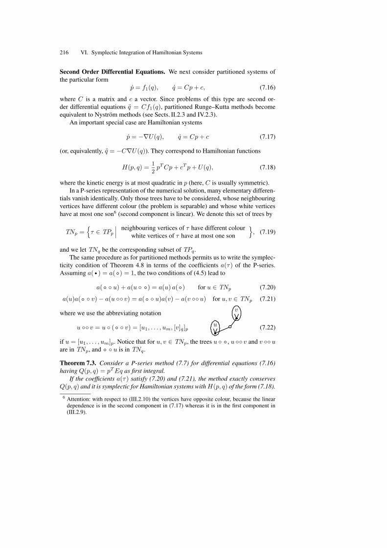
Up to now in this chapter, we have presented sufficient conditions for the symplec-ticity of numerical integrators (usually in terms of certain coefficients). Here, wewill prove necessary conditions for symplecticity, i.e., answer the question as towhich methods are not symplectic. It will turn out that the sufficient conditions ofSect. VI.4, under an irreducibility condition on the method, are also necessary. Themain tool is the Taylor series expansion of the numerical flow y0 7→ Φh(y0), whichwe assume to be a B-series (or a P-series).
VI.7.1 B-Series Methods Conserving Quadratic First Integrals
The numerical solution of a Runge–Kutta method (II.1.4) can be written as aB-series
y1 = B(a, y0) = y0 +∑
τ∈T
h|τ |
σ(τ)a(τ)F (τ)(y0) (7.1)
with coefficients a(τ) given by
a(τ) =s∑
i=1
bigi(τ) for τ ∈ T (7.2)
(see (III.1.16) and Sect. III.1.2). Our aim is to express the sufficient condition forthe exact conservation of quadratic first integrals (which is the same as for symplec-ticity) in terms of the coefficients a(τ). For this we multiply (4.2) by gi(u) · gj(v)(where u = [u1, . . . , um] and v = [v1, . . . , vl] are trees in T ) and we sum over all iand j. Using (III.1.13) and the recursion (III.1.15) this yields
s∑
i=1
bigi(u v) +s∑
j=1
bjgj(v u) =( s∑
i=1
bigi(u))( s∑
j=1
bjgj(v)),
where we have used the Butcher product (see, e.g., Butcher (1987), Sect. 143)
u v = [u1, . . . , um, v], v u = [v1, . . . , vl, u] (7.3)
(compare also Definition III.3.7 and Fig. 7.1 below). Because of (7.2), this implies
a(u v) + a(v u) = a(u) · a(v) for u, v ∈ T. (7.4)
We now forget that the B-series (7.1) has been obtained from a Runge–Kuttamethod, and we ask the following question: is the condition (7.4) sufficient for aB-series method defined by (7.1) to conserve exactly quadratic first integrals (andto be symplectic)? The next theorem shows that this is indeed true, and we shall seelater that condition (7.4) is also necessary (cf. Chartier, Faou & Murua 2005).
VI.7 Characterization of Symplectic Methods 213
Theorem 7.1. Consider a B-series method Φh(y) = B(a, y) and problemsy = f(y) having Q(y) = yTCy (with symmetric matrix C) as first integral.
If the coefficients a(τ) satisfy (7.4), then the method exactly conservesQ(y) andit is symplectic.
Proof. a) Under the assumptions of the theorem we shall prove in part (c) that
B(a, y)TCB(a, y) = yTCy+∑
u,v∈T
h|u|+|v|
σ(u)σ(v)m(u, v)F (u)(y)TCF (v)(y) (7.5)
with m(u, v) = a(u) · a(v) − a(u v) − a(v u). Condition (7.4) is equivalent tom(u, v) = 0 and thus implies the exact conservation of Q(y) = yTCy.
To prove symplecticity of the method it is sufficient to show that the diagram ofLemma 4.1 commutes for general B-series methods. This is seen by differentiatingthe elementary differentials and by comparing them with those for the augmentedsystem (Exercise 8). Symplecticity of the method thus follows as in Sect. VI.4.1form the fact that the symplecticity relation is a quadratic first integral of the aug-mented system.
b) Since Q(y) = yTCy is a first integral of y = f(y), we have yTCf(y) = 0for all y. Differentiating m times this relation with respect to y yields
m∑
j=1
kTj Cf
(m−1)(y)(k1, . . . , kj−1, kj+1 . . . , km
)+yTCf (m)(y)
(k1, . . . , km) = 0.
Putting kj = F (τj)(y) we obtain the formula
yTCF ([τ1, . . . , τm])(y) = −m∑
j=1
F (τj)(y)TCF ([τ1, . . . , τj−1, τj+1, . . . , τm])(y),
which can also be written in the form
yTCF (τ)(y)
σ(τ)= −
∑
u,v∈T,vu=τ
F (u)(y)T
σ(u)CF (v)(y)
σ(v). (7.6)
c) With (7.1) the expression yT1 Cy1 becomes
B(a, y)TCB(a, y) = yTCy + 2yTC∑
τ∈T
h|τ |
σ(τ)a(τ)F (τ)(y)
+∑
u,v∈T
h|u|+|v|
σ(u)σ(v)a(u) a(v)F (u)(y)TCF (v)(y).
Since C is symmetric, formula (7.6) remains true if we sum over trees u, v such thatu v = τ . Inserting both formulas into the sum over τ leads directly to (7.5). ut
214 VI. Symplectic Integration of Hamiltonian Systems
Extension to P-Series. All the previous results can be extended to partitioned meth-ods. To find the correct conditions on the coefficients of the P-series, we use the factthat the numerical solution of a partitioned Runge–Kutta method (II.2.2) is a P-series
(p1
q1
)=
(Pp(a, (p0, q0))
Pq(a, (p0, q0))
)=
(p0
q0
)+
(∑u∈TPp
h|u|
σ(u) a(u)F (u)(p0, q0)∑
v∈TPq
h|v|
σ(v) a(v)F (v)(p0, q0)
)
(7.7)with coefficients a(τ) given by
a(τ) =
∑si=1 biφi(τ) for τ ∈ TPp∑si=1 biφi(τ) for τ ∈ TPq
(7.8)
(see Theorem III.2.4). We assume here that the elementary differentials F (τ)(p, q)originate from a partitioned sytem
p = f1(p, q), q = f2(p, q), (7.9)
such as the Hamiltonian system (1.7). This time we multiply (4.3) by φi(u) · φj(v)(where u = [u1, . . . , um]p ∈ TPp and v = [v1, . . . , vl]q ∈ TPq) and we sum overall i and j. Using the recursion (III.2.7) this yields
s∑
i=1
biφi(u v) +
s∑
j=1
bjφj(v u) =( s∑
i=1
biφi(u))( s∑
j=1
bjφj(v)), (7.10)
where u v = [u1, . . . , um, v]p and v u = [v1, . . . , vl, u]q . Because of (7.8), thisimplies the relation
a(u v) + a(v u) = a(u) · a(v) for u ∈ TPp, v ∈ TPq. (7.11)
Since φi(τ) is independent of the colour of the root of τ , condition (4.4) implies
a(τ) is independent of the colour of the root of τ . (7.12)
Theorem 7.2. Consider a P-series method (p1, q1) = Φh(p0, q0) given by (7.7),and a problem (7.9) having Q(p, q) = pTE q as first integral.
i) If the coefficients a(τ) satisfy (7.11) and (7.12), the method exactly conservesQ(p, q) and it is symplectic for general Hamiltonian systems (1.7).
ii) If the coefficients a(τ) satisfy only (7.11), the method exactly conservesQ(p, q) for problems of the form p = f1(q), q = f2(p), and it is symplectic forseparable Hamiltonian systems where H(p, q) = T (p) + U(q).
Proof. This is very similar to that of Theorem 7.1. If Q(p, q) = pTE q is a firstintegral of (7.9), we have f1(p, q)
TE q + pTE f2(p, q) = 0 for all p and q. Differ-entiating m times with respect to p and n times with respect to q yields
VI.7 Characterization of Symplectic Methods 215
0 = Dmp D
nq f1(p, q)
(k1, . . . , km, `1, . . . , `n
)TE q
+ pTEDmp D
nq f2(p, q)
(k1, . . . , km, `1, . . . , `n
)(7.13)
+
n∑
j=1
Dmp D
n−1q f1(p, q)
(k1, . . . , km, `1, . . . , `j−1, `j+1, . . . , `n
)TE `j
+m∑
i=1
kTi ED
m−1p Dn
q f2(p, q)(k1, . . . , ki−1, ki+1, . . . , km, `1, . . . , `n
).
Putting ki = F (ui)(p, q) with ui ∈ TPp, `j = F (vj)(p, q) with vj ∈ TPq, τp =[u1, . . . , um, v1, . . . , vn]p and τq = [u1, . . . , um, v1, . . . , vn]q, we obtain as in part(b) of the proof of Theorem 7.1 that
F (τp)(p, q)T
σ(τp)E q + pTE
F (τq)(p, q)
σ(τq)(7.14)
=∑
uv=τp
F (u)(p, q)T
σ(u)EF (v)(p, q)
σ(v)+
∑
vu=τq
F (u)(p, q)T
σ(u)EF (v)(p, q)
σ(v),
where the sums are over u ∈ TPp and v ∈ TPq.With (7.7) the expression pT
1 E q1 becomes
Pp(a, (p, q))TE Pq(a, (p, q)) = pTE q (7.15)
+∑
u∈TPp
h|u|
σ(u)a(u)F (u)(p, q)TE q + pTE
∑
v∈TPq
h|v|
σ(v)a(v)F (v)(p, q)
+∑
u∈TPp,v∈TPq
h|u|+|v|
σ(u)σ(v)a(u)a(v)F (u)(p, q)TE F (v)(p, q).
Condition (7.12) implies that a(τp) = a(τq) for the trees in (7.14). Since also |τp| =|τq| and σ(τp) = σ(τq), two corresponding terms in the sums of the second linein (7.15) can be jointly replaced by the use of (7.14). As in part (c) of the proof ofTheorem 7.1 this together with (7.11) then yields
Pp(a, (p, q))TE Pq(a, (p, q)) = pTE q,
which proves the conservation of quadratic first integrals pTE q. Symplecticity fol-lows as before, because the diagram of Lemma 4.1 also commutes for general P-series methods.
For the proof of statement (ii) we notice that f1(q)TE q + pTE f2(p) = 0 im-
plies that f1(q)TE q = 0 and pTE f2(p) = 0 vanish separately. Instead of (7.14)we thus have two identities: the term F (τp)(p, q)
TE q/σ(τp) becomes equal to thefirst sum in (7.14), and pTE F (τq)(p, q)/σ(τq) to the second sum. Consequently,the previous argumentation can be applied without the condition a(τp) = a(τq). ut
216 VI. Symplectic Integration of Hamiltonian Systems
Second Order Differential Equations. We next consider partitioned systems ofthe particular form
p = f1(q), q = Cp+ c, (7.16)
where C is a matrix and c a vector. Since problems of this type are second or-der differential equations q = Cf1(q), partitioned Runge–Kutta methods becomeequivalent to Nystrom methods (see Sects. II.2.3 and IV.2.3).
An important special case are Hamiltonian systems
p = −∇U(q), q = Cp+ c (7.17)
(or, equivalently, q = −C∇U(q)). They correspond to Hamiltonian functions
H(p, q) =1
2pTCp+ cT p+ U(q), (7.18)
where the kinetic energy is at most quadratic in p (here, C is usually symmetric).In a P-series representation of the numerical solution, many elementary differen-
tials vanish identically. Only those trees have to be considered, whose neighbouringvertices have different colour (the problem is separable) and whose white verticeshave at most one son6 (second component is linear). We denote this set of trees by
TNp =τ ∈ TPp
∣∣∣ neighbouring vertices of τ have different colourwhite vertices of τ have at most one son
, (7.19)
and we let TNq be the corresponding subset of TPq.The same procedure as for partitioned methods permits us to write the symplec-
ticity condition of Theorem 4.8 in terms of the coefficients a(τ) of the P-series.Assuming a( ) = a( ) = 1, the two conditions of (4.5) lead to
a( u) + a(u ) = a(u) a( ) for u ∈ TNp (7.20)
a(u)a( v) − a(u v) = a( u)a(v) − a(v u) for u, v ∈ TNp (7.21)
where we use the abbreviating notation
u v = u ( v) = [u1, . . . , um, [v]q]pu
v
(7.22)
if u = [u1, . . . , um]p. Notice that for u, v ∈ TNp, the trees u , u v and v uare in TNp, and u is in TNq .
Theorem 7.3. Consider a P-series method (7.7) for differential equations (7.16)having Q(p, q) = pTEq as first integral.
If the coefficients a(τ) satisfy (7.20) and (7.21), the method exactly conservesQ(p, q) and it is symplectic for Hamiltonian systems withH(p, q) of the form (7.18).
6 Attention: with respect to (III.2.10) the vertices have opposite colour, because the lineardependence is in the second component in (7.17) whereas it is in the first component in(III.2.9).
VI.7 Characterization of Symplectic Methods 217
Proof. Since the elementary differentials F (τ)(p, q) vanish identically for τ 6∈TNp ∪ TNq , we can arbitrarily define a(τ) for trees outside TNp ∪ TNq with-out changing the method (throughout this proof we implicitly assume that for theconsidered trees neighbouring vertices have different colour). We shall do this insuch a way that (7.11) holds.
Consider first the tree u v. There is exactly one vertex between the roots of uand v. Making this vertex to the root gives the tree [u, v]q which is not in TNq . Wedefine for u, v ∈ TNp
a([u, v]q) := a(u)a( v) − a(u v).
Condition (7.21) shows that a([u, v]q) is independent of permuting u and v and isthus well-defined. For trees that are neither in TNp ∪ TNq nor of the form [u, v]qwith u, v ∈ TNp we let a(τ) = 0. This extension of a(τ) implies that condition(7.11) holds for all trees, and part (ii) of Theorem 7.2 yields the statement. Noticethat for problems p = f1(q), q = f2(p) only trees, for which neighbouring verticeshave different colour, are relevant. ut
VI.7.2 Characterization of Symplectic P-Series (and B-Series)
A characterization of symplectic B-series was first obtained by Calvo & Sanz-Serna(1994). We also consider P-series with various important special situations.
Theorem 7.4. Consider a P-series method (7.7) applied to a general partitioneddifferential equation (7.9). Equivalent are:
1) the coefficients a(τ) satisfy (7.11) and (7.12),2) quadratic first integrals of the form Q(p, q) = pTE q are exactly conserved,3) the method is symplectic for general Hamiltonian systems (1.7).
Proof. The implication (1)⇒(2) follows from part (i) of Theorem 7.2, (2)⇒(3) is aconsequence of the fact that the symplecticity condition is a quadratic first integral ofthe variational equation (see the proof of Theorem 7.2). The remaining implication(3)⇒(1) will be proved in the following two steps.
a) We fix two trees u ∈ TPp and v ∈ TPq, and we construct a (polynomial)Hamiltonian such that the transformation (7.7) satisfies
(∂(p1, q1)
∂p10
)T
J(∂(p1, q1)
∂q20
)= C
(a(u v) + a(v u) − a(u) · a(v)
)(7.23)
with C 6= 0 (here, p10 denotes the first component of p0, and q20 the second compo-
nent of q0). The symplecticity of (7.7) implies that the expression in (7.23) vanishes,so that condition (7.11) has to be satisfied.
For given u ∈ TPp and v ∈ TPq we define the Hamiltonian as follows: to thebranches of u v we attach the numbers 3, . . . , |u| + |v| + 1 such that the branchbetween the roots of u and v is labelled by 3. Then, the Hamiltonian is a sum ofas many terms as vertices in the tree. The summand corresponding to a vertex is a
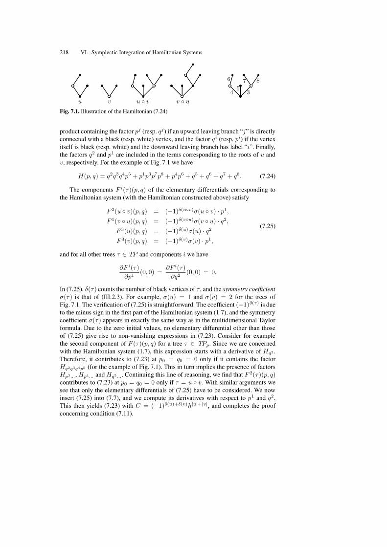
218 VI. Symplectic Integration of Hamiltonian Systems
u v u v v u34
5
6 7 8
Fig. 7.1. Illustration of the Hamiltonian (7.24)
product containing the factor pj (resp. qj) if an upward leaving branch “j” is directlyconnected with a black (resp. white) vertex, and the factor qi (resp. pi) if the vertexitself is black (resp. white) and the downward leaving branch has label “i”. Finally,the factors q2 and p1 are included in the terms corresponding to the roots of u andv, respectively. For the example of Fig. 7.1 we have
H(p, q) = q2q3q4p5 + p1p3p7p8 + p4p6 + q5 + q6 + q7 + q8. (7.24)
The components F i(τ)(p, q) of the elementary differentials corresponding tothe Hamiltonian system (with the Hamiltonian constructed above) satisfy
F 2(u v)(p, q) = (−1)δ(uv)σ(u v) · p1,
F 1(v u)(p, q) = (−1)δ(vu)σ(v u) · q2,F 3(u)(p, q) = (−1)δ(u)σ(u) · q2F 3(v)(p, q) = (−1)δ(v)σ(v) · p1,
(7.25)
and for all other trees τ ∈ TP and components i we have
∂F i(τ)
∂p1(0, 0) =
∂F i(τ)
∂q2(0, 0) = 0.
In (7.25), δ(τ) counts the number of black vertices of τ , and the symmetry coefficientσ(τ) is that of (III.2.3). For example, σ(u) = 1 and σ(v) = 2 for the trees ofFig. 7.1. The verification of (7.25) is straightforward. The coefficient (−1)δ(τ) is dueto the minus sign in the first part of the Hamiltonian system (1.7), and the symmetrycoefficient σ(τ) appears in exactly the same way as in the multidimensional Taylorformula. Due to the zero initial values, no elementary differential other than thoseof (7.25) give rise to non-vanishing expressions in (7.23). Consider for examplethe second component of F (τ)(p, q) for a tree τ ∈ TPp. Since we are concernedwith the Hamiltonian system (1.7), this expression starts with a derivative of Hq2 .Therefore, it contributes to (7.23) at p0 = q0 = 0 only if it contains the factorHq2q3q4p5 (for the example of Fig. 7.1). This in turn implies the presence of factorsHp3...,Hp4... and Hq5.... Continuing this line of reasoning, we find that F 2(τ)(p, q)contributes to (7.23) at p0 = q0 = 0 only if τ = u v. With similar arguments wesee that only the elementary differentials of (7.25) have to be considered. We nowinsert (7.25) into (7.7), and we compute its derivatives with respect to p1 and q2.This then yields (7.23) with C = (−1)δ(u)+δ(v)h|u|+|v|, and completes the proofconcerning condition (7.11).
VI.7 Characterization of Symplectic Methods 219
b) The necessity of condition (7.12) is seen similarly. We fix a tree τ ∈ TPp
and we let τ ∈ TPq be the tree obtained from τ by changing the colour of the root.We then attach the numbers 3, . . . , |τ | + 1 to the branches of τ , and we define aHamiltonian as above but, different from adding the factors q2 and p1, we includethe factor p1q2 to the term corresponding to the root. For the tree τ = u of Fig. 7.1this yields
H(p, q) = p1q2q3p4 + p3p5 + q4 + q5.
With this Hamiltonian we get
F 2(τ)(p, q) = (−1)δ(τ)σ(τ) · p1,
F 1(τ)(p, q) = (−1)δ(τ)σ(τ) · q2,and these are the only elementary differentials contributing to the left-hand expres-sion of (7.23). We thus get
(∂(p1, q1)
∂p10
)T
J(∂(p1, q1)
∂q20
)= (−1)δ(τ)h|τ |
(a(τ) − a(τ)
),
which completes the proof of Theorem 7.4. ut
Theorem 7.5. Consider a P-series method (7.7) applied to a separable partitioneddifferential equation p = f1(q), q = f2(p). Equivalent are:
1) the coefficients a(τ) satisfy (7.11),2) quadratic first integrals of the form Q(p, q) = pTE q are exactly conserved,3) the method is symplectic for separable HamiltoniansH(p, q) = T (p)+U(q).
Proof. The implications (1)⇒(2)⇒(3) follow as before from part (ii) of Theo-rem 7.2. The remaining implication (3)⇒(1) is a consequence of the fact that theHamiltonian constructed in part (a) of the proof of Theorem 7.4 is separable, whenu and v have no neighbouring vertices of the same colour. ut
Theorem 7.6. Consider a B-series method (7.1) for y = f(y). Equivalent are:1) the coefficients a(τ) satisfy (7.4),2) quadratic first integrals of the form Q(y) = yTCy are exactly conserved,3) the method is symplectic for general Hamiltonian systems y = J−1∇H(y).
Proof. The implications (1)⇒(2)⇒(3) follow from Theorem 7.1. The remainingimplication (3)⇒(1) follows from Theorem 7.4, because a B-series with coefficientsa(τ), τ ∈ T , applied to a partitioned differential equation, can always be interpretedas a P-series (Definition III.2.1), where a(τ) := a(ϕ(τ)) for τ ∈ TP and ϕ : TP →T is the mapping that forgets the colouring of the vertices. This follows from thefact that
α(τ)F (τ)(y) =
(∑u∈TPp,ϕ(u)=τ α(u)F (u)(p, q)∑v∈TPq ,ϕ(v)=τ α(v)F (v)(p, q)
)
for τ ∈ T , because α(u) · σ(u) = α(v) · σ(v) = e(τ) · |τ |! . Here, y = (p, q), theelementary differentials F (τ)(y) are those of Definition III.1.2, whereas F (u)(p, q)and F (v)(p, q) are those of Table III.2.1. ut
220 VI. Symplectic Integration of Hamiltonian Systems
Theorem 7.7. Consider a P-series method (7.7) applied to the special partitionedsystem (7.16). Equivalent are:
1) the coefficients a(τ) satisfy (7.20) and (7.21),2) quadratic first integrals of the form Q(p, q) = pTE q are exactly conserved,3) the method is symplectic for Hamiltonian systems of the form (7.17).
Proof. The implications (1)⇒(2)⇒(3) follow from Theorem 7.3. The remainingimplication (3)⇒(1) can be seen as follows.
Condition (7.20) is a consequence of the the proof of Theorem 7.4, because foru ∈ TNp and v = the Hamiltonian constructed there is of the form (7.18).
To prove condition (7.21) we have to modify slightly the definition of H(p, q).We take u, v ∈ TNp and define the polynomial Hamiltonian as follows: to thebranches of u v we attach the numbers 3, . . . , |u| + |v| + 2. The Hamiltonian isthen a sum of as many terms as vertices in the tree. The summands are defined as inthe proof of Theorem 7.4 with the only exception that to the terms corresponding tothe roots of u and v we include the factors q2 and q1, respectively, instead of q2 andp1. This gives a Hamiltonian of the form (7.18), for which the expression
(∂(p1, q1)
∂q10
)T
J(∂(p1, q1)
∂q20
)(7.26)
becomes equal to
a(u)a( v) − a(u v) − a( u)a(v) + a(v u) (7.27)
up to a nonzero constant. By symplecticity, (7.26) is zero so that also (7.27) has tovanish. This proves the validity of condition (7.21). ut
VI.7.3 Irreducible Runge–Kutta Methods
We are now able to study to what extent the conditions of Theorem 4.3 and Theo-rem 4.6 are also necessary for symplecticity. Consider first the 2-stage method
1/2 α 1/2 − α
1/2 β 1/2 − β
1/2 1/2
.
The solution of the corresponding Runge–Kutta system (II.1.4) is given by k1 =k2 = k, where k = f(y0 +k/2), and hence y1 = y0 +hk. Whatever the values of αand β are, the numerical solution of the Runge–Kutta method is identical to that ofthe implicit midpoint rule, so that it defines a symplectic transformation. However,the condition (4.2) is only satisfied for α = β = 1/4.
Definition 7.8. Two stages i and j of a Runge–Kutta method (II.1.4) are said to beequivalent for a class (P) of initial value problems, if for every problem in (P) andfor every sufficiently small step size we have ki = kj (ki = kj and `i = `j forpartitioned Runge–Kutta methods (II.2.2)).
VI.7 Characterization of Symplectic Methods 221
The method is called irreducible for (P) if it does not have equivalent stages.It is called irreducible if it is irreducible for all sufficiently smooth initial valueproblems.
For a more amenable characterization of irreducible Runge–Kutta methods, weintroduce an ordering on T (and on TP ), and we consider the following s × ∞matrices
ΦRK =(φ(τ); τ ∈ T
)with entries φi(τ) = gi(τ) given by (III.1.13),7
ΦPRK =(φ(τ); τ ∈ TPp
)=(φ(τ); τ ∈ TPq
)with entries φi(τ) given by (III.2.7);
observe that φi(τ) does not depend on the colour of the root,Φ∗
PRK =(φ(τ); τ ∈ TP ∗
p
)=(φ(τ); τ ∈ TP ∗
q
)where TP ∗
p (resp. TP ∗q ) is the set
of trees in TPp (resp. TPq) whose neighbouring vertices have different colours.
Lemma 7.9 (Hairer 1994). A Runge–Kutta method is irreducible if and only if thematrix ΦRK has full rank s.
A partitioned Runge–Kutta method is irreducible if and only if the matrix ΦPRKhas full rank s.
A partitioned Runge–Kutta method is irreducible for separable problems p =f1(q), q = f2(p) if and only if the matrix Φ∗
PRK has full rank s.
Proof. If the stages i and j are equivalent, it follows from the expansion
ki =∑
τ∈T
h|τ |
σ(τ)φi(τ)F (τ)(y0)
(see the proof of Theorem III.1.4) and from the independency of the elementarydifferentials (Exercise III.3) that φi(τ) = φj(τ) for all τ ∈ T . Hence, the rowsi and j of the matrix ΦRK are identical. The analogous statement for partitionedRunge–Kutta methods follows from Theorem III.2.4 and Exercise III.6. This provesthe sufficiency of the ‘full rank’ condition.
We prove its necessity only for partitioned Runge–Kutta methods applied to sep-arable problems (the other situations can be treated similarly). For separable prob-lems, only trees in TP ∗
p ∪ TP ∗q give rise to non-vanishing elementary differentials.
Irreducibility therefore implies that for every pair (i, j) with i 6= j there exists a treeτ ∈ TP ∗
p such that φi(τ) 6= φj(τ). Consequently, a certain finite linear combina-tion of the columns of Φ∗
PRK has distinct elements, i.e., there exist vectors ξ ∈ R∞
(only finitely many non zero elements) and η ∈ Rs with Φ∗
PRKξ = η and ηi 6= ηj
for i 6= j. Due to the fact that φi([τ1, . . . , τm]) = φi([τ1]) · . . . · φi([τm]), the com-ponentwise product of two columns of Φ∗
PRK is again a column of Φ∗PRK. Continuing
this argumentation and observing that (1, . . . , 1)T is a column of Φ∗PRK, we obtain
a matrix X such that Φ∗PRKX = (ηj−1
i )si,j=1 is a Vandermonde matrix. Since the ηi
are distinct, the matrix Φ∗PRK has to be of full rank s. ut
7 In this section we let φ(τ) ∈ Rs denote the vector whose elements are φi(τ), i = 1, . . . , s.
This should not be mixed up with the value φ(τ) of (III.1.16).
222 VI. Symplectic Integration of Hamiltonian Systems
VI.7.4 Characterization of Irreducible Symplectic MethodsThe necessity of the condition (4.2) for symplectic Runge–Kutta methods was firststated by Lasagni (1988). Abia & Sanz-Serna (1993) extended his proof to parti-tioned methods. We follow here the ideas of Hairer (1994).
Theorem 7.10. An irreducible Runge–Kutta method (II.1.4) is symplectic if andonly if the condition (4.2) holds.
An irreducible partitioned Runge–Kutta method (II.2.2) is symplectic if and onlyif the conditions (4.3) and (4.4) hold.
A partitioned Runge–Kutta method, irreducible for separable problems, is sym-plectic for separable Hamiltonians H(p, q) = T (p)+U(q) if and only if the condi-tion (4.3) holds.
Proof. The “if” part of all three statements has been proved in Theorem 4.3 andTheorem 4.6. We prove the “only if” part for partitioned Runge–Kutta methodsapplied to general Hamiltonian systems (the other two statements can be obtainedin the same way).
We consider the s × s matrix M with entries mij = biaij + bjaji − bibj . Thecomputation leading to formula (7.11) shows that for u ∈ TPp and v ∈ TPq
φ(u)TM φ(v) = a(u v) + a(v u) − a(u) · a(v)holds. Due to the symplecticity of the method, this expression vanishes and weobtain
ΦTPRKM ΦPRK = 0,
where ΦPRK is the matrix of Lemma 7.9. An application of this lemma then yieldsM = 0, which proves the necessity of (4.3).
For the vector d with components di = bi − bi we get dTΦPRK = 0, and wededuce from Lemma 7.9 that d = 0, so that (4.4) is also seen to be necessary. ut
VI.8 Conjugate SymplecticityThe symplecticity requirement may be too strong if we are interested in a correctlong-time behaviour of a numerical integrator. Stoffer (1988) suggests consideringmethods that are not necessarily symplectic but conjugate to a symplectic method.
Definition 8.1. Two numerical methods Φh and Ψh are mutually conjugate, if thereexists a global change of coordinates χh, such that
Φh = χ−1h Ψh χh. (8.1)
We assume that χh(y) = y + O(h) uniformly for y varying in a compact set.
For a numerical solution yn+1 = Φh(yn), lying in a compact subset of thephase space, the transformed values zn = χh(yn) constitute a numerical solutionzn+1 = Ψh(zn) of the second method. Since yn − zn = O(h), both numericalsolutions have the same long-time behaviour, independently of whether one methodshares certain properties (e.g., symplecticity) with the other.
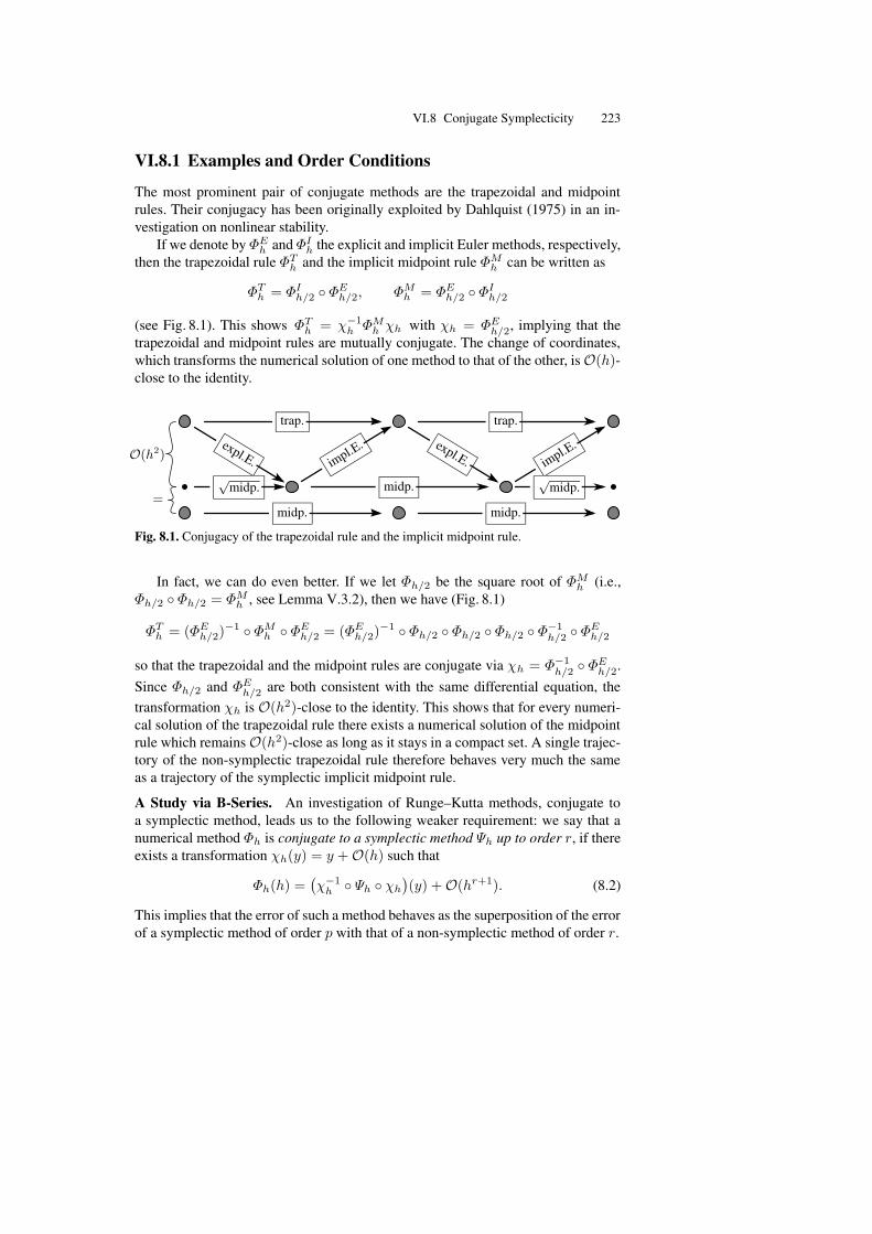
VI.8 Conjugate Symplecticity 223
VI.8.1 Examples and Order Conditions
The most prominent pair of conjugate methods are the trapezoidal and midpointrules. Their conjugacy has been originally exploited by Dahlquist (1975) in an in-vestigation on nonlinear stability.
If we denote by ΦEh and ΦI
h the explicit and implicit Euler methods, respectively,then the trapezoidal rule ΦT
h and the implicit midpoint rule ΦMh can be written as
ΦTh = ΦI
h/2 ΦEh/2, ΦM
h = ΦEh/2 ΦI
h/2
(see Fig. 8.1). This shows ΦTh = χ−1
h ΦMh χh with χh = ΦE
h/2, implying that thetrapezoidal and midpoint rules are mutually conjugate. The change of coordinates,which transforms the numerical solution of one method to that of the other, is O(h)-close to the identity.
trap. trap.
expl.E.expl.E.impl.E.
impl.E.
√midp. midp.
√midp.
midp. midp.
O(h2)
=
Fig. 8.1. Conjugacy of the trapezoidal rule and the implicit midpoint rule.
In fact, we can do even better. If we let Φh/2 be the square root of ΦMh (i.e.,
Φh/2 Φh/2 = ΦMh , see Lemma V.3.2), then we have (Fig. 8.1)
ΦTh = (ΦE
h/2)−1 ΦM
h ΦEh/2 = (ΦE
h/2)−1 Φh/2 Φh/2 Φh/2 Φ−1
h/2 ΦEh/2
so that the trapezoidal and the midpoint rules are conjugate via χh = Φ−1h/2 ΦE
h/2.Since Φh/2 and ΦE
h/2 are both consistent with the same differential equation, thetransformation χh is O(h2)-close to the identity. This shows that for every numeri-cal solution of the trapezoidal rule there exists a numerical solution of the midpointrule which remains O(h2)-close as long as it stays in a compact set. A single trajec-tory of the non-symplectic trapezoidal rule therefore behaves very much the sameas a trajectory of the symplectic implicit midpoint rule.
A Study via B-Series. An investigation of Runge–Kutta methods, conjugate toa symplectic method, leads us to the following weaker requirement: we say that anumerical method Φh is conjugate to a symplectic method Ψh up to order r, if thereexists a transformation χh(y) = y + O(h) such that
Φh(h) =(χ−1
h Ψh χh
)(y) + O(hr+1). (8.2)
This implies that the error of such a method behaves as the superposition of the errorof a symplectic method of order p with that of a non-symplectic method of order r.
224 VI. Symplectic Integration of Hamiltonian Systems
In the following we assume that all methods considered as well as the conjugacymapping χh can be represented as B-series
Φh(y) = B(a, y), Ψh(y) = B(b, y), χh(y) = B(c, y). (8.3)
Using the composition formula (III.1.38) of B-series, condition (8.2) becomes
(ac)(τ) = (cb)(τ) for |τ | ≤ r. (8.4)
The following results are taken from the thesis of P. Leone (2000).
Theorem 8.2. Let Φh(y) = B(a, y) represent a numerical method of order 2.a) It is always conjugate to a symplectic method up to order 3.b) It is conjugate to a symplectic method up to order 4, if and only if
a( , ) − 2a( , ) = 0, a( , ) − 2a( , ) = 0. (8.5)
Here, we use the abbreviation a(u, v) = a(u) · a(v) − a(u v) − a(v u).Proof. The condition (8.4) allows us to express b(τ) as a function of a(u) for |u| ≤|τ | and of c(v) for |v| ≤ |τ |−1 (use the formulas of Example III.1.11). All we haveto do is to check the symplecticity conditions b(u, v) = 0 for |u| + |v| ≤ r (seeTheorem 7.6).
Since the method Φh is of order 2, we obtain b( ) = 1 and b( ) = 1/2. Wearbitrarily fix c( ) = 0, so that the symplecticity condition b( , ) = 0 becomes2c( ) = a( , ). Defining c( ) by this relation proves statement (a).
For order 4, the three symplecticity conditions b( , ) = b( , [[ ]]) =b( , ) = 0 have to be fulfilled. One of them can be satisfied by defining suit-ably c( ) + c([[ ]]); the other two conditions are then equivalent to (8.5). utTheorem 8.3. Let Φh(y) = B(a, y) represent a numerical method of order 4. It isconjugate to a symplectic method up to order 5, if and only if
a( , ) − 2a( , ) = 0, a( , ) − 3a( , ) + 3a( , ) = 0,
a( , ) − a( , ) − 2a( , ) + 3a( , ) = 0.
Proof. The idea of the proof is the same as in the preceding theorem. The verifica-tion is left as an exercise for the reader. utExample 8.4. A direct computation shows that for the Lobatto IIIB method withs = 3 we have a( , ) = 1/144, and a(u, v) = 0 for all other pairs with|u| + |v| = 5. Theorem 8.3 therefore proves that this method is not conjugate toa symplectic method up to order 5.
For the Lobatto IIIA method with s = 3 we obtain a( , ) = −1/144,a( , [[ ]]) = −1/288, and a(u, v) = 0 for the remaining pairs with |u| + |v| = 5.This time the conditions of Theorem 8.3 are fulfilled, so that the Lobatto IIIAmethod with s = 3 is conjugate to a symplectic method up to order 5 at least.
VI.8 Conjugate Symplecticity 225
VI.8.2 Near Conservation of Quadratic First IntegralsWe have already met in Sect. VI.4.1 a close relationship between symplecticity andthe conservation of quadratic first integrals. The aim of this section is to show asimilar connection between conjugate symplecticity and the near conservation ofquadratic first integrals. This has first been observed and proved by Chartier, Faou& Murua (2005) using the algebra of rooted trees.
Let Q(y) = yTCy (with symmetric matrix C) be a quadratic first integral ofy = f(y), and assume that Φh(y) is conjugate to a method Ψh(y) that exactly con-serves quadratic first integrals (e.g., symplectic Runge–Kutta methods). This meansthat yn+1 = Φh(yn) satisfies
χh(yn+1)TCχh(yn+1) = χh(yn)TCχh(yn),
and the expression Q(y) = χh(y)TCχh(y) is exactly conserved by the numericalsolution of Φh(y). If χh(y) = B(c, y) is a B-series, this is of the form
Q(y) =∑
τ,ϑ∈T∪∅
h|τ |+|ϑ|β(τ, ϑ)F (τ)(y)TC F (ϑ)(y), (8.6)
where F (∅)(y) = y and |∅| = 0 for the empty tree, and β(∅, ∅) = 1. We havethe following criterion for conjugate symplecticity, where all formulas have to beinterpreted in the sense of formal series.
Theorem 8.5. Assume that a one-step method Φh(y) = B(a, y) leaves (8.6) invari-ant for all problems y = f(y) having Q(y) = yTCy as first integral.
Then, it is conjugate to a symplectic integrator Ψh(z), i.e., there exists a transfor-mation z = χh(y) = B(c, y) such that Ψh(z) = χh Φh χ−1
h (z), or equivalently,Ψh(z) = B(c−1ac, z) is symplectic.
Proof. The idea is to search for a B-series B(c, y) such that the expression (8.6)becomes
Q(y) = B(c, y)TC B(c, y).
The mapping z = χh(y) = B(c, y) then provides a change of variables such thatthe original first integral Q(z) = zTCz is invariant in the new variables. By Theo-rem 7.6 this then implies that Ψh is symplectic.
By Lemma 8.6 below, the expression (8.6) can be written as
Q(y) = yTC(y +
∑
θ∈T
h|θ|η(θ)F (θ)(y)), (8.7)
where η(θ) = 0 for |θ| < r, if the perturbation in (8.6) is of size O(hr). Using thesame lemma once more, we obtain
B(c, y)TC B(c, y) = yTC(y + 2
∑
θ∈T
h|θ|
σ(θ)c(θ)F (θ)(y)
)
+ yTC(∑
θ∈T
( h|θ|σ(θ)
∑
τ,ϑ∈T
σ(θ)κτ,ϑ(θ)
σ(τ)σ(ϑ)c(τ)c(ϑ)F (θ)(y)
).
(8.8)
226 VI. Symplectic Integration of Hamiltonian Systems
A comparison of the coefficients in (8.7) and (8.8) uniquely defines c(θ) in a recur-sive manner. We have c(θ) = 0 for |θ| < r, so that the transformation z = B(c, y)is O(hr) close to the identity. ut
The previous proof is based on the following result.
Lemma 8.6. Let Q(y) = yTCy (with symmetric matrix C) be a first integral ofy = f(y). Then, for every pair of trees τ, ϑ ∈ T , we have
F (τ)(y)TC F (ϑ)(y) = yTC(∑
θ∈T
κτ,ϑ(θ)F (θ)(y)).
This sum is finite and only over trees satisfying |θ| = |τ | + |ϑ|.Proof. By definition of a first integral we have yTC f(y) = 0 for all y. Differentia-tion with respect to y gives
f(y)TC k + yTC f ′(y)k = 0 for all k. (8.9)
Putting k = F (ϑ)(y), this proves the statement for τ = .Differentiating once more yields
(f ′(y)`)TC k + `TC f ′(y)k + yTC f ′′(y)(k, `) = 0.
Putting ` = f(y) and using (8.9), we get the statement for τ = . With ` =F (τ1)(y) we obtain the statement for τ = [τ1] provided that it is already proved forτ1. We need a further differentiation to get a similar statement for τ = [τ1, τ2], etc.The proof concludes by induction on the order of τ . utPartitioned Methods. This criterion for conjugate symplecticity can be extendedto partitioned P-series methods. For partitioned problems
p = f1(p, q), q = f2(p, q) (8.10)
we consider first integrals of the form L(p, q) = pTE q, where E is an arbitraryconstant matrix. If Φh(p, q) is conjugate to a method that exactly conserves L(p, q),then it will conserve a modified first integral of the form
L(p, q) =∑
τ∈TPp∪∅p,ϑ∈TPq∪∅q
h|τ |+|ϑ|β(τ, ϑ)F (τ)(p, q)TE F (ϑ)(p, q), (8.11)
where β(∅p, ∅q) = 1, F (∅p)(p, q) = p, F (∅q)(p, q) = q. We first extend Lemma 8.6to the new situation.
Lemma 8.7. Let L(p, q) = pTE q be a first integral of (8.10). Then, for every pairof trees τ ∈ TPp, ϑ ∈ TPq , we have
F (τ)(p, q)TE F (ϑ)(p, q) = pTE( ∑
θ∈TPq
κτ,ϑ(θ)F (θ)(p, q))
+( ∑
θ∈TPp
κτ,ϑ(θ)F (θ)(p, q))T
E q.(8.12)
These sums are finite and only over trees satisfying |θ| = |τ | + |ϑ|.
VI.9 Volume Preservation 227
Proof. Since L(p, q) = pTE q is a first integral of the differential equation, wehave f1(p, q)TE q+pTE f2(p, q) = 0 for all p and q. As in the proof of Lemma 8.6the statement follows from differentiation of this relation. utTheorem 8.8. Assume that a partitioned one-step method Φh(p, q) = P (a, (p, q))leaves (8.11) invariant for all problems (8.10) having L(p, q) = pTE q as firstintegral.
Then it is conjugate to a symplectic integrator Ψh(u, v), i.e., there is a transfor-mation (u, v) = χh(p, q) = P (c, (p, q)) such that Ψh(u, v) = χh Φh χ−1
h (u, v),or equivalently, Ψh(u, v) = P (c−1ac, (u, v)) is symplectic.
Proof. We search for a P-series P (c, (p, q)) =(Pp(c, (p, q)), Pq(c, (p, q))
)T suchthat the expression (8.11) can be written as
L(p, q) = Pp(c, (p, q))TE Pq(c, (p, q)).
As in the proof of Theorem 8.5 the mapping (u, v) = χh(p, q) = P (c, (p, q)) thenprovides the searched change of variables.
Using Lemma 8.7 the expression (8.11) becomes
L(p, q) = pTE(q +
∑
θ∈TPq
h|θ|η(θ)F (θ)(p, q))
+( ∑
θ∈TPp
h|θ|η(θ)F (θ)(p, q))T
E q.
Also Pp(c, (p, q))TE Pq(c, (p, q)) can be written in such a form, and a comparison
of the coefficients yields the coefficients c(τ) of the P-series P (c, (p, q)) in a recur-sive manner. We again have that P (c, (p, q)) is O(hr) close to the identity, if theperturbation in (8.11) is of size O(hr). ut
The statement of Theorem 8.8 remains true in the class of second order differ-ential equations q = f1(q), i.e., p = f1(p), q = p.
VI.9 Volume PreservationThe flow ϕt of a Hamiltonian system preserves volume in phase space: for everybounded open set Ω ⊂ R
2d and for every t for which ϕt(y) exists for all y ∈ Ω,
vol(ϕt(Ω)) = vol(Ω) ,
where vol(Ω) =∫
Ωdy. This identity is often referred to as Liouville’s theorem. It
is a consequence of the transformation formula for integrals and the fact that
det∂ϕt(y)
∂y= 1 for all t and y, (9.1)
which follows directly from the symplecticity and ϕ0 = id. The same argumentshows that every symplectic transformation, and in particular every symplectic in-tegrator applied to a Hamiltonian system, preserves volume in phase space.
More generally than for Hamiltonian systems, volume is preserved by the flowof differential equations with a divergence-free vector field:
228 VI. Symplectic Integration of Hamiltonian Systems
Lemma 9.1. The flow of a differential equation y=f(y) in Rn is volume-preserving
if and only if divf(y) = 0 for all y.
Proof. The derivative Y (t) = ∂ϕt
∂y (y0) is the solution of the variational equation
Y = A(t)Y , Y (0) = I ,
with the Jacobian matrix A(t) = f ′(y(t)) at y(t) = ϕt(y0). From the proof ofLemma IV.3.1 we obtain the Abel–Liouville–Jacobi–Ostrogradskii identity
d
dtdetY = traceA(t) · detY. (9.2)
Note that here traceA(t) = divf(y(t)). Hence, detY (t) = 1 for all t if and only ifdivf(y(t)) = 0 for all t. Since this is valid for all choices of initial values y0, theresult follows. ut
Example 9.2 (ABC Flow). This flow, named after the three independent authorsArnold, Beltrami and Childress, is given by the equations
x = A sin z + C cos y
y = B sinx+A cos z
z = C sin y +B cosx
(9.3)
and has all diagonal elements of f ′ identically zero. It is therefore volume preserv-ing. In Arnold (1966, p. 347) it appeared in a footnote as an example of a flow withrotf parallel to f , thus violating Arnold’s condition for the existence of invarianttori (Arnold 1966, p. 346). It was therefore expected to possess interesting chaoticproperties and has since then been the object of many investigations showing theirnon-integrability (see e.g., Ziglin (1996)). We illustrate in Fig. 9.1 the action of thisflow by transforming, in a volume preserving manner, a ball in R
3. We see that,very soon, the set is strongly squeezed in one direction and dilated in two others.The solutions thus depend in a very sensitive way on the initial values.
Volume-Preserving Numerical Integrators. The question arises as to whethervolume-preserving integrators can be constructed for every differential equationwith volume-preserving flow. Already for linear problems, Lemma IV.3.2 showsthat no standard method can be volume-preserving for dimension n ≥ 3. Never-theless, positive answers were found by Qin & Zhu (1993), Shang (1994a,1994b),Feng & Shang (1995) and Quispel (1995). In the following we present the approachof Feng & Shang (1995). The key is the following result which generalizes andreinterprets a construction of H. Weyl (1940) for n = 3.
Theorem 9.3 (Feng & Shang 1995). Every divergence-free vector field f : Rn →
Rn can be written as the sum of n− 1 vector fields
f = f1,2 + f2,3 + . . .+ fn−1,n
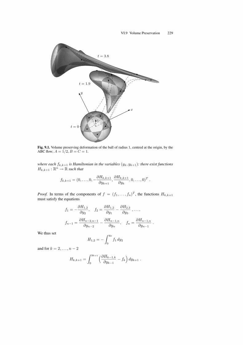
VI.9 Volume Preservation 229
x
y
z
t = 0
t = 1.9
t = 3.8
Fig. 9.1. Volume preserving deformation of the ball of radius 1, centred at the origin, by theABC flow; A = 1/2, B = C = 1.
where each fk,k+1 is Hamiltonian in the variables (yk, yk+1): there exist functionsHk,k+1 : R
n → R such that
fk,k+1 = (0, . . . , 0,−∂Hk,k+1
∂yk+1,∂Hk,k+1
∂yk, 0, . . . , 0)T .
Proof. In terms of the components of f = (f1, . . . , fn)T , the functions Hk,k+1
must satisfy the equations
f1 = −∂H1,2
∂y2, f2 =
∂H1,2
∂y1− ∂H2,3
∂y3, . . . ,
fn−1 =∂Hn−2,n−1
∂yn−2− ∂Hn−1,n
∂yn, fn =
∂Hn−1,n
∂yn−1.
We thus set
H1,2 = −∫ y2
0
f1 dy2
and for k = 2, . . . , n− 2
Hk,k+1 =
∫ yk+1
0
(∂Hk−1,k
∂yk−1− fk
)dyk+1 .
230 VI. Symplectic Integration of Hamiltonian Systems
It remains to construct Hn−1,n from the last two equations. We see by inductionthat for k ≤ n− 2,
∂2Hk,k+1
∂yk∂yk+1= −
(∂f1∂y1
+ . . .+∂fk
∂yk
),
and hence the integrability condition for Hn−1,n,
∂
∂yn−1
(∂Hn−2,n−1
∂yn−2− fn−1
)=∂fn
∂yn,
reduces to the condition divf = 0, which is satisfied by assumption. Hn−1,n canthus be constructed as
Hn−1,n =
∫ yn
0
(∂Hn−2,n−1
∂yn−2− fn−1
)dyn +
∫ yn−1
0
fn|yn=0 dyn−1 ,
which completes the proof. ut
The above construction also shows that
fk,k+1 = (0, . . . , 0, fk + gk,−gk+1, 0, . . . , 0)
with
gk+1 =
∫ yk+1
0
(∂f1∂y1
+ . . .+∂fk
∂yk
)dyk+1
for 1 ≤ k ≤ n− 2, and g1 = 0 and gn = −fn.With the decomposition of Lemma 9.3 at hand, a volume-preserving algorithm
is obtained by applying a splitting method with symplectic substeps. For example,as proposed by Feng & Shang (1995), a second-order volume-preserving method isobtained by Strang splitting with symplectic Euler substeps:
ϕh ≈ Φh = Φ[1,2]∗h/2 . . . Φ[n−1,n]∗
h/2 Φ[n−1,n]h/2 . . . Φ[1,2]
h/2
where Φ[k,k+1]h/2 is a symplectic Euler step of length h/2 applied to the system with
right-hand side fk,k+1, and ∗ denotes the adjoint method. In this method, one stepy = Φh(y) is computed component-wise, in a Gauss-Seidel-like manner, as
y1 = y1 +h
2f1(y1, y2, . . . , yn)
yk = yk +h
2fk(y1, . . . , yk, yk+1, . . . , yn) +
h
2gk|yk
ykfor k = 2, . . . , n− 1
yn = yn +h
2fn(y1, . . . , yn−1, yn) (9.4)
with gk|ykyk = gk(y1, . . . , yk, yk+1, . . . , yn) − gk(y1, . . . , yk−1, yk, . . . , yn), and
VI.9 Volume Preservation 231
yn = yn +h
2fn(y1, . . . , yn)
yk = yk +h
2fk(y1, . . . , yk, yk+1 . . . , yn) − h
2gk|byk
ykfor k = n− 1, . . . , 2
y1 = y1 +h
2f1(y1, y2, . . . , yn) (9.5)
with gk|byk
yk= gk(y1, . . . , yk−1, yk, . . . , yn) − gk(y1, . . . , yk, yk+1, . . . , yn). The
method is one-dimensionally implicit in general, but becomes explicit in the par-ticular case where ∂fk/∂yk = 0 for all k.
Separable Partitioned Systems. For problems of the form
y = f(z), z = g(y) (9.6)
with y ∈ Rm, z ∈ R
n, the scheme (9.4) becomes the symplectic Euler method, (9.5)its adjoint, and its composition the Lobatto IIIA - IIIB extension of the Stormer–Verlet method. Since symplectic explicit partitioned Runge–Kutta methods are com-positions of symplectic Euler steps (Theorem VI.4.7), this observation proves thatsuch methods are volume-preserving for systems (9.6). This fact was obtained bySuris (1996) by a direct calculation, without interpreting the methods as composi-tion methods. The question arises as to whether more symplectic partitioned Runge–Kutta methods are volume-preserving for systems (9.6).
Theorem 9.4. Every symplectic Runge–Kutta method with at most two stages isvolume-preserving for systems (9.6) of arbitrary dimension.
Proof. (a) The idea is to consider the Hamiltonian system with
H(u, v, y, z) = uT f(z) + vT g(y),
where (u, v) are the conjugate variables to (y, z). This system is of the form
y = f(z)
z = g(y)
u = −g′(y)T v
v = −f ′(z)Tu.(9.7)
Applying the Runge–Kutta method to this augmented system does not change thenumerical solution for (y, z). For symplectic methods the matrix
(∂(y1, z1, u1, v1)
∂(y0, z0, u0, v0)
)= M =
(R 0S T
)(9.8)
satisfies MTJM = J which implies RT T = I . Below we shall show that detT =detR. This yields detR = 1 which implies that the method is volume preserving.
(b) One-stage methods. The only symplectic one-stage method is the implicitmidpoint rule for which R and T are computed as
232 VI. Symplectic Integration of Hamiltonian Systems
(I − h
2E1
)R = I +
h
2E1 (9.9)
(I +
h
2ET
1
)T = I − h
2ET
1 , (9.10)
where E1 is the Jacobian of the system (9.6) evaluated at the internal stage value.Since
E1 =
(0 f ′(z1/2)
g′(y1/2) 0
),
a similarity transformation with the matrix D = diag(I,−I) takes E1 to −E1.Hence, the transformed matrix satisfies
(I − h
2ET
1
)(D−1TD) = I +
h
2ET
1 .
A comparison with (9.9) and the use of detXT = detX proves detR = detT forthe midpoint rule.
(c) Two-stage methods. Applying a two-stage implicit Runge–Kutta method to(9.7) yields (
I − ha11E1 −ha12E2
−ha21E1 I − ha22E2
)(R1
R2
)=
(II
),
where Ri is the derivative of the (y, z) components of the ith stage with respect to(y0, z0), and Ei is the Jacobian of the system (9.6) evaluated at the ith internal stagevalue. From the solution of this system the derivative R of (9.8) is obtained as
R = I + (b1E1, b2E2)
(I − ha11E1 −ha12E2
−ha21E1 I − ha22E2
)−1(II
).
With the determinant identity
det(U) det(X −WU−1V ) = det
(U VW X
)= det(X) det(U − V X−1W ),
which is seen by Gaussian elimination, this yields
detR =det(I ⊗ I − h((A− 1lbT ) ⊗ I)E
)
det(I ⊗ I − h(A⊗ I)E
) ,
where A and b collect the Runge–Kutta coefficients, and E = blockdiag (E1, E2).For D−1TD we get the same formula with E replaced by ET . If A is an arbitrary2 × 2 matrix, it follows from block Gaussian elimination that
det(I ⊗ I − h(A⊗ I)E
)= det
(I ⊗ I − h(A⊗ I)ET
), (9.11)
which then proves detR = detT . Notice that the identity (9.11) is no longer truein general if A is of dimension larger than two. ut
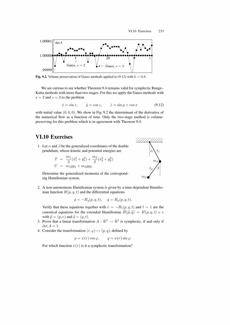
VI.10 Exercises 233
20
.99999
1.00000
1.00001
t
detA
Gauss, s = 2 Gauss, s = 3
Fig. 9.2. Volume preservation of Gauss methods applied to (9.12) with h = 0.8.
We are curious to see whether Theorem 9.4 remains valid for symplectic Runge–Kutta methods with more than two stages. For this we apply the Gauss methods withs = 2 and s = 3 to the problem
x = sin z, y = cos z, z = sin y + cosx (9.12)
with initial value (0, 0, 0). We show in Fig. 9.2 the determinant of the derivative ofthe numerical flow as a function of time. Only the two-stage method is volume-preserving for this problem which is in agreement with Theorem 9.4.
VI.10 Exercises1. Let α and β be the generalized coordinates of the double
pendulum, whose kinetic and potential energies are
T =m1
2(x2
1 + y21) +
m2
2(x2
2 + y22)
U = m1gy1 +m2gy2.
Determine the generalized momenta of the correspond-ing Hamiltonian system.
m1
`1α
m2
`2 β
2. A non-autonomous Hamiltonian system is given by a time-dependent Hamilto-nian function H(p, q, t) and the differential equations
p = −Hq(p, q, t), q = Hp(p, q, t).
Verify that these equations together with e = −Ht(p, q, t) and t = 1 are thecanonical equations for the extended Hamiltonian H(p, q) = H(p, q, t) + ewith p = (p, e) and q = (q, t).
3. Prove that a linear transformation A : R2 → R
2 is symplectic, if and only ifdetA = 1.
4. Consider the transformation (r, ϕ) 7→ (p, q), defined by
p = ψ(r) cosϕ, q = ψ(r) sinϕ.
For which function ψ(r) is it a symplectic transformation?
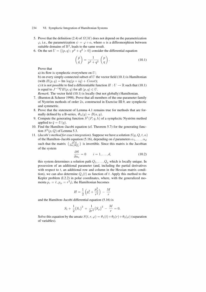
234 VI. Symplectic Integration of Hamiltonian Systems
5. Prove that the definition (2.4) of Ω(M) does not depend on the parametrizationϕ, i.e., the parametrization ψ = ϕ α, where α is a diffeomorphism betweensuitable domains of R
2, leads to the same result.6. On the set U = (p, q) ; p2 + q2 > 0 consider the differential equation
(pq
)=
1
p2 + q2
(pq
). (10.1)
Prove thata) its flow is symplectic everywhere on U ;b) on every simply-connected subset of U the vector field (10.1) is Hamiltonian(with H(p, q) = Im log(p+ iq) + Const);c) it is not possible to find a differentiable functionH : U → R such that (10.1)is equal to J−1∇H(p, q) for all (p, q) ∈ U .Remark. The vector field (10.1) is locally (but not globally) Hamiltonian.
7. (Burnton & Scherer 1998). Prove that all members of the one-parameter familyof Nystrom methods of order 2s, constructed in Exercise III.9, are symplecticand symmetric.
8. Prove that the statement of Lemma 4.1 remains true for methods that are for-mally defined by a B-series, Φh(y) = B(a, y).
9. Compute the generating function S1(P, q, h) of a symplectic Nystrom methodapplied to q = U(q).
10. Find the Hamilton–Jacobi equation (cf. Theorem 5.7) for the generating func-tion S2(p,Q) of Lemma 5.3.
11. (Jacobi’s method for exact integration). Suppose we have a solution S(q,Q, t, α)of the Hamilton–Jacobi equation (5.16), depending on d parameters α1, . . . , αd
such that the matrix(
∂2S∂αi∂Qj
)is invertible. Since this matrix is the Jacobian
of the system∂S
∂αi= 0 i = 1, . . . , d, (10.2)
this system determines a solution path Q1, . . . , Qq which is locally unique. Inpossession of an additional parameter (and, including the partial derivativeswith respect to t, an additional row and column in the Hessian matrix condi-tion), we can also determine Qj(t) as function of t. Apply this method to theKepler problem (I.2.2) in polar coordinates, where, with the generalized mo-menta pr = r, pϕ = r2ϕ, the Hamiltonian becomes
H =1
2
(p2
r +p2
ϕ
r2
)− M
r
and the Hamilton–Jacobi differential equation (5.16) is
St +1
2
(Sr
)2+
1
2r2(Sϕ
)2 − M
r= 0.
Solve this equation by the ansatz S(t, r, ϕ) = θ1(t)+θ2(r)+θ3(ϕ) (separationof variables).
VI.10 Exercises 235
Result. One obtains
S =
∫ √2α1r2 + 2Mr − α2
2
dr
r+ α2ϕ− α1t.
Putting, e.g., ∂S/∂α2 = 0, we obtain ϕ = arcsinMr−α2
2√M2+2α1α2
2r
by evaluating
an elementary integral. This, when resolved for r, leads to the elliptic movementof Kepler (Sect. I.2.2). This method turned out to be most effective for the exactintegration of difficult problems. With the same ideas, just more complicatedin the computations, Jacobi solves in “lectures” 24 through 30 of (Jacobi 1842)the Kepler motion in R
3, the geodesics of ellipsoids (his greatest triumph), themotion with two centres of gravity, and proves a theorem of Abel.
12. (Chan’s Lobatto IIIS methods.) Show that there exists a one-parameter familyof symplectic, symmetric (and A-stable) Runge–Kutta methods of order 2s− 2based on Lobatto quadrature (Chan 1990). A special case of these methods canbe obtained by taking the arithmetic mean of the Lobatto IIIA and Lobatto IIIBmethod coefficients (Sun 2000).Hint. Use theW -transformation (see Hairer & Wanner (1996), p. 77) by puttingXs,s−1 = −Xs−1,s an arbitrary constant.
13. For a Hamiltonian system with associated Lagrangian L(q, q) = 12 q
TMq −U(q), show that every first integral I(p, q) = pTa(q) resulting from Noether’sTheorem has a linear a(q) = Aq + c with skew-symmetric MA.Hint. (a) It is sufficient to consider the case M = I .(b) Show that a′(q) is skew-symmetric.(c) Let aij(q) = ∂ai
∂qj(q). Using the symmetry of the Hessian of each compo-
nent ai(q), show that aij(q) does not depend on qi, qj , and is at most linear inthe remaining components qk. With the skew-symmetry of a′(q), conclude thata′(q) = Const .
14. Consider the unconstrained optimal control problem
C(q(T )
)→ min
q(t) = f(q(t), u(t)
), q(0) = q0
(10.3)
on the interval [0, T ], where the control function is assumed to be continuous.Prove that first-order necessary optimality conditions can be written as
q(t) = ∇pH(p(t), q(t), u(t)
), q(0) = q0
p(t) = −∇qH(p(t), q(t), u(t)
), p(T ) = ∇qC
(q(T )
)
0 = ∇uH(p(t), q(t), u(t)
),
(10.4)
where the Hamiltonian is given by
H(p, q, u) = pT f(q, u)
(we assume that the Hessian ∇2uH(p, q, u) is invertible, so that the third relation
of (10.4) defines u as a function of (p, q)).
236 VI. Symplectic Integration of Hamiltonian Systems
Hint. Consider a slightly perturbed control function u(t) + εδu(t), and letq(t)+εδq(t)+O(ε2) be the corresponding solution of the differential equationin (10.3). With the function p(t) of (10.4) we then have
C ′(q(T )
)δq(T ) =
∫ T
0
d
dt
(p(t)T δq(t)
)dt =
∫ T
0
p(t)T fu
(. . .)δu(t)dt.
The algebraic relation of (10.4) then follows from the fundamental lemma ofvariational calculus.
15. A Runge–Kutta discretization of the problem (10.3) is
C(qN ) → min
qn+1 = qn + h∑s
i=1 bif(Qni, Uni)
Qni = qn + h∑s
j=1 aijf(Qnj , Unj)
(10.5)
with n = 0, . . . , N − 1 and h = T/N . We assume bi 6= 0 for all i. Introducingsuitable Lagrange multipliers for the constrained minimization problem (10.5),prove that there exist pn, Pni such that the optimal solution of (10.5) satisfies(Hager 2000)
qn+1 = qn + h∑s
i=1 bi∇pH(Pni, Qni, Uni)
Qni = qn + h∑s
j=1 aij∇pH(Pnj , Qnj , Unj)
pn+1 = pn − h∑s
i=1 bi∇qH(Pni, Qni, Uni)
Pni = pn − h∑s
j=1 aij∇qH(Pnj , Qnj , Unj)
0 = ∇uH(Pni, Qni, Uni)
(10.6)
with pN = ∇qC(qN ) and given initial value q0, where the coefficients bi andaij are determined by
bi = bi, biaij + bjaji = bibj . (10.7)
Consequently, (10.6) can be considered as a symplectic discretization of (10.4);see Bonnans & Laurent-Varin (2006).
16. (Hager 2000). For an explicit s-stage Runge–Kutta method of order p = s andbi 6= 0, consider the partitioned Runge–Kutta method with additional coeffi-cients bi and aij defined by (10.7). Prove the following:a) For p = s = 3, the partitioned method is of order 3 if and only if c3 = 1.b) For p = s = 4, the partitioned method is of order 4 without any restriction.