Explicit Multi-Symplectic Extended Leap-frog Methods …xiaj/work/MSERKN.pdf · Explicit...

Explicit Multi-Symplectic Extended Leap-frog Methods for HamiltonianWave Equations

Wei Shia, Xinyuan Wua, Jianlin Xiab,∗

aDepartment of Mathematics, Nanjing University; State Key Laboratory for Novel Software Technology at Nanjing University, Nanjing210093, P.R.China

bDepartment of Mathematics, Purdue University, West Lafayette, IN 47907, USA

Abstract

In this paper, we study the integration of Hamiltonian wave equations whose solutions have oscillatory be-haviors in time and/or space. We are mainly concerned with the research for multi-symplectic extendedRunge-Kutta-Nystrom (ERKN) discretizations and the corresponding discrete conservation laws. We firstshow that the discretizations to the Hamiltonian wave equations using two symplectic ERKN methods inspace and time respectively lead to an explicit multi-symplectic integrator (Eleap-frogI). Then we derive an-other multi-symplectic discretization using a symplectic ERKN method in time and a symplectic PartitionedRunge-Kutta method, which is equivalent to the well-known Stormer-Verlet method in space (Eleap-frogII).These two new multi-symplectic schemes are extensions of the leap-frog method. The numerical stabilityand dispersive properties of the new schemes are analyzed. Numerical experiments with comparisons arepresented, where the two new explicit multi-symplectic methods and the leap-frog method are applied to thelinear wave equation and the sine-Gordon equation. The numerical results confirm the superior performanceand some significant advantages of our new integrators in the sense of structure preservation.

Keywords: Multi-symplectic integrators, Hamiltonian wave equations, extended leap-frog methods,conservation laws, dispersive properties

Mathematics Subject Classification (2000): 35L05, 37M15, 65L06, 65M12, 65P10, 70S10

1. Introduction

It is well-known that symplectic integrators are robust, efficient, and accurate in preserving the long-time behavior of the solutions of Hamiltonian ordinary differential equations (ODEs) [1]. The basic ideaof a symplectic integrator is that the numerical scheme is designed to preserve the symplectic form at eachtime step. Recently, it is shown that many conservative partial differential equations (PDEs), such as waveequations, generalized KdV and nonlinear Schrodinger equations, etc., allow for a structure similar to thesymplectic structure of Hamiltonian ODEs, called the multi-symplectic formulation (see, e.g., [2, 3, 4]). Forexample, in [4], Marsden and Shkoller develop the multi-symplectic structure of Hamiltonian PDEs from aLagrangian formulation using a variational principle.

It is natural to design integrators for Hamiltonian PDEs which preserve a semi-discretization of the sym-plectic form associated with the infinite-dimensional evolution equation. In the past decade, rapid progress

IThe research of Wei Shi and Xinyuan Wu was supported in part by the Natural Science Foundation of China under Grant 10771099and by the Specialized Research Foundation for the Doctoral Program of Higher Education under Grant 20100091110033, by the 985Project at Nanjing University under Grant 9112020301, by A Project Founded by the Priority Academic Program Development ofJiangsu Higher Education Institutions, and by the University Postgraduate Research and Innovation Project of Jiangsu Province 2012under Grant CXLX12−0033.

IIThe research of Jianlin Xia was supported in part by NSF grants DMS-1115572 and CHE-0957024.∗Corresponding author.Email address: [email protected], [email protected], [email protected] (Jianlin Xia)

1

W. Shi, X. Wu, and J. Xia 2

has been made on the development of multi-symplectic integrators of Runge-Kutta type for various Hamil-tonian PDEs (see, e.g., [5, 6, 7, 8, 9, 10, 11, 12]). Unfortunately, most of the existing multi-symplecticintegrators fail to take into account the oscillatory behavior of the problems of interest, which is importantfor the solution that has the intrinsic oscillatory behavior.

It is known that most of integrators adapted to the oscillatory problems are frequency-dependent, such asARKN methods [13, 14, 15, 16, 17], ERKN methods [18, 19, 20, 21], and trigonometrically/exponentially-fitted methods [22, 23, 24, 25]. For nonlinear Schrodinger equations, taking the frequency of the probleminto account, several useful trigonometrically/exponentially-fitted methods are proposed (see, e.g., [26, 27,28, 29, 30, 31, 32]). Some authors, such as Gonzalez, et al. [33] and Franco [13], are interested in numericalintegrators of Runge-Kutta-Nystrom type adapted to initial value problems of the form

y′′(t) + ω2y(t) = f

(y(t)

), t ∈ [t0,T ],

y(t0) = y0, y′(t0) = y′0,(1)

where ω is the main frequency and ω > 0. More recently, a new family of extended Runge-Kutta-Nystrom(ERKN) methods are proposed by Yang, et al. [18] for one-dimensional perturbed oscillators and systemsof these oscillators with ω2 being a diagonal matrix. Furthermore, with the methodology in [18], a standardform of multidimensional ERKN integrators for the general system (1) is formulated by Wu, et al. [19], whereω2 is a symmetric positive semi-definite matrix and implicitly contains the frequencies of the problem. Thecorresponding order conditions are also derived by the authors based on the B-series theory associated withthe extended Nystrom trees (EN-trees) [19]. These methods preserve the oscillatory feature of the unperturbedoscillators, not only for the updates but also for the internal stages. Numerical results have shown that ERKNmethods are superior to other methods for oscillatory systems.

In this paper, we investigate the multi-symplectic ERKN (MSERKN) methods for wave equations asHamiltonian PDEs. In Section 2, we discuss the conservation laws for Hamiltonian wave equations. In Sec-tion 3, we show that the discretization in time and space for Hamiltonian wave equations with two symplecticERKN (SERKN) methods leads to a multi-symplectic integrator. In Section 4, explicit multi-symplecticschemes are constructed based on the SERKN methods and a symplectic Partitioned Runge-Kutta (SPRK)method. Section 5 is devoted to the numerical experiments, including the dispersive properties of the schemesproposed in this paper. Some conclusions are given in the last section.

2. Conservation laws and multi-symplectic structures of wave equations

2.1. Multi-symplectic conservation laws and multi-symplectic integrators

A multi-Hamiltonian PDE in one time dimension and one space dimension is a PDE that can be formu-lated in the following way (see [34]). Let M and K be any skew-symmetric real n × n matrices (n ≥ 3) andlet S : Rn → R be any smooth function of the state variable z. Then a system of the following form is calleda Hamiltonian system on a multi-symplectic structure:

Mzt + Kzx = ∇zS (z), z ∈ Rn, (x, t) ∈ R2, (2)

where ∇z is the gradient operator corresponding to the standard inner product on Rn denoted by 〈·, ·〉.The Hamiltonian system (2) is multi-symplectic in the sense that it is associated with two-forms:

ζ =12

dz ∧ Mdz, κ =12

dz ∧ Kdz,

which define a space-time symplectic structure governed by the multi-symplectic conservation law

∂tζ + ∂xκ = 0. (3)

Let L be the length of the spatial domain. Then integrating (3) over the spatial domain leads to

ddt

∫ L/2

−L/2ζdx + κ|x=L/2 − κ|x=−L/2 = 0.


This equation, under appropriate boundary conditions such as z(L/2, t) = z(−L/2, t), results in the conserva-

tion of global symplecticity:ddtζ(z) = 0, where

ζ(z) =

∫ L/2

−L/2ζ(z)dx. (4)

ζ(z) is a reminder indicating that the two-form ζ is integrated over all space. A properly chosen semi-discretization of this system may lead to a system of Hamiltonian ODEs with a symplectic form given bya discrete version of (4). An overview of this viewpoint in terms of symplectic time-integration methods isgiven by McLachlan [35].

Two other conservation laws for the energy and the momentum respectively follow from (3). The localenergy conservation law is

∂tE(z) + ∂xF(z) = 0, (5)

where E(z) = S (z)− 12

zT Kzx is the energy density and F(z) =12

zT Kzt is the energy flux. The local momentumconservation law is

∂tI(z) + ∂xG(z) = 0, (6)

where I(z) =12

zT Mzx and G(z) = S (z) − 12

zT Mzt are the momentum density and the momentum flux,respectively. Similar to the conservation of multi-symplecticity, integrating the local conservation laws (5)and (6) over the spatial domain in Rn with periodic boundary conditions leads to global conservation laws

ddtε(z) = 0 and

ddtI(z) = 0, (7)

where ε(z) =∫ L/2−L/2 E(z)dx and I(z) =

∫ L/2−L/2 I(z)dx. We note that the global conservation of energy or

momentum (7) is necessary but not sufficient for the local conservation of energy or momentum.When it comes to the numerical integration, the symplecticity of numerical integrators should be deter-

mined.

Definition 2.1. [34] A numerical scheme is called multi-symplectic if it preserves a discrete conservationlaw of (3).

An alternative definition of multi-symplectic integrators based on a discrete form of the symplectic con-servation law is suggested by Bridges and Reich [3]. It has been shown that popular methods such as thecentered Preissman scheme and the leap-frog method are multi-symplectic and that such schemes have re-markable properties of conserving local energy and momentum.

2.2. Conservation laws for wave equations

Consider the following nonlinear wave equation (see [36]):

utt − uxx + V ′(u) = 0, (8)

where V(u) is certain smooth function and u is a scalar function. Introducing two new variables v = ut andw = ux, we can write (8) as

vt − wx + V ′(u) = 0,v = ut,w = ux.

By taking z = (u, v,w)T ∈ R3, we can obtain a first order PDE system of the abstract form (2) correspondingto (8) (see, e.g., [11]), with

M =

0 −1 01 0 00 0 0

, K =

0 0 10 0 0−1 0 0

,


and the Hamiltonian is S (z) =12

(v2 − w2) + V(u). As mentioned in Subsection 2.1, this system has themulti-symplectic conservation law (3), where ζ and κ are the pre-symplectic forms

ζ =12

dz ∧ Mdz = dv ∧ du, (9)

κ =12

dz ∧ Kdz = du ∧ dw. (10)

By applying the general approach of deriving the local energy and momentum conservation law to thenonlinear wave equation (8), as discussed in the previous subsection, it follows that the local energy conserva-

tion law is (5) with E(z) =12

(v2 + w2) + V(u) and F(z) = −vw. Meanwhile, the local momentum conservation

law is (6) with I(z) = vw and G(z) = −12

(v2 + w2) + V(u) (see [11]).

3. Extended RKN discretization of wave equations

3.1. Extended RKN methods for ODEs

In [18], Yang, et al. investigate ERKN methods for the IVP (1) of the following form :

Yi = φ0(ciν)yn + ciφ1(ciν)hy′n + h2s∑

j=1ai j(ν) f (tn + c jh,Y j), i = 1, . . . , s,

yn+1 = φ0(ν)yn + φ1(ν)hy′n + h2s∑

i=1bi(ν) f (tn + cih,Yi),

y′n+1 = −νwφ1(ν)yn + φ0(ν)y′n + hs∑

i=1bi(ν) f (tn + cih,Yi),

(11)

where ai j(ν), bi(ν) and bi(ν), i, j = 1, . . . , s, are assumed to be even functions of ν = hω, φ0(ν) = cos(ν), and

φ1(ν) =sin(ν)ν

. We denote (11) by ci, bi, bi, ai j, ω in this paper.Very recently, ERKN methods are considered for Hamiltonian ODEs, whose solutions exhibit a periodic

or oscillatory character. The coefficients of these methods depend on the product of the step size h and thefitted frequency ω, and the methods can be expressed in Butcher tableau as :

c A(ν)

bT (ν)

bT (ν)

=

c1 a11(ν) . . . a1s(ν)...

.... . .

...cs as1(ν) · · · ass(ν)

b1(ν) · · · bs(ν)

b1(ν) · · · bs(ν)

The symplecticity conditions for ERKN methods are given by the next theorem.

Theorem 3.1. (Wu, et al. [37, 20]) If the coefficients of an s-stage ERKN method satisfy the followingconditions

bi(ν)(φ0(ν) +

ciν2φ1(ν)φ1(ciν)φ0(ciν)

)= bi(ν)

(φ1(ν) − ciφ0(ν)φ1(ciν)

φ0(ciν)

),

i = 1, . . . , s,

bi(ν)(

b j(ν) − ai j(ν)φ0(ν)φ0(ciν)

)− bi(ν)ai j(ν)

ν2φ1(ν)φ0(ciν)

= b j(ν)(

bi(ν) − a ji(ν)φ0(ν)φ0(c jν)

)− b j(ν)a ji(ν)

ν2φ1(ν)φ0(c jν)

, i, j = 1, . . . , s,

(12)

then the method is symplectic.


R 3.1. When ω→ 0, the scheme (11) reduces to a classical RKN method in Hairer, et al. [38]. Inthis case, the symplecticity conditions of (12) become

bi = (1 − ci)bi, i = 1, . . . , s,bi(b j − ai j) = b j(bi − a ji), i ≤ j = 1, . . . , s,

which are obtained by Suris [39] for the symplecticity of an s-stage RKN method.

3.2. Multi-symplectic extended RKN discretization

In order to derive the new MSERKN methods, we first consider the discretization of the equation (8) byemploying the following two different SERKN methods in temporal and spatial directions, respectively:

c1 a11(νt) . . . a1r(νt)...

.... . .

...cr ar1(νt) · · · arr(νt)

b1(νt) · · · br(νt)

b1(νt) · · · br(νt)

c1 a11(νx) . . . a1s(νx)...

.... . .

...cs as1(νx) · · · ass(νx)

b1(νx) · · · bs(νx)

b1(νx) · · · bs(νx)

Theorem 3.2. Assume that a method results from the temporal discretization of the wave equation (8) with anr-stage SERKN scheme ci, bi, bi, ai j, ωt and spatial discretization with an s-stage SERKN scheme ci, bi, bi,ai j, ωx, where the coefficients satisfy the symplectic conditions

bi(νt)(φ0(νt) +

ciνt2φ1(νt)φ1(ciνt)φ0(ciνt)

)= bi(νt)

(φ1(νt) − ciφ0(νt)φ1(ciνt)

φ0(ciνt)

),

i = 1, . . . , r,

bi(νt)(

b j(νt) − ai j(νt)φ0(νt)φ0(ciνt)

)− bi(νt)ai j(νt)

νt2φ1(νt)φ0(ciνt)

= b j(νt)(

bi(νt) − a ji(νt)φ0(νt)φ0(c jνt)

)− b j(νt)a ji(νt)

νt2φ1(νt)φ0(c jνt)

,

i, j = 1, . . . , r,

(13)

and

bi(νx)(φ0(νx) +

ciνx2φ1(νx)φ1(ciνx)φ0(ciνx)

)= bi(νx)

(φ1(νx) − ciφ0(νx)φ1(ciνx)

φ0(ciνx)

),

i = 1, . . . , s,

bi(νx)(

b j(νx) − ai j(νx)φ0(νx)φ0(ciνx)

)− bi(νx)ai j(νx)

νx2φ1(νx)φ0(ciνx)

= b j(νx)(

bi(νx) − a ji(νx)φ0(νx)φ0(c jνx)

)− b j(νx)a ji(νx)

νx2φ1(νx)

φ0(c jνx),

i, j = 1, . . . , s,

(14)

respectively. The method is said to be multi-symplectic in the sense that it satisfies the discrete multi-symplectic conservation law

s∑i=1

(1

φ0(ciνx)(biφ0(νx) + biν

2xφ1(νx)

))(dvn+1

m,i ∧ dun+1m,i − dvn

m,i ∧ dunm,i)h

+r∑

k=1

(1

φ0(ckνt)(bkφ0(νt) + bkν

2t φ1(νt)

))(dun,k

m+1 ∧ dwn,km+1 − dun,k

m ∧ dwn,km )τ = 0,

(15)

where τ and h are the step-size of time and space, respectively.


Proof. We first apply an s-stage SERKN method with the spatial discretization and rewrite equation(8) as

Ui = φ0(ciνx)um + ciφ1(ciνx)hwm + h2s∑

j=1ai j(νx) f j, i = 1, . . . , s,

um+1 = φ0(νx)um + φ1(νx)hwm + h2s∑

i=1bi(νx) fi,

wm+1 = −νxωxφ1(νx)um + φ0(νx)wm + hs∑

i=1bi(νx) fi,

where fi = f (Ui) = ω2xUi + ∂xxUi. Having φ0(ν) = cos(ν) and φ1(ν) =

sin(ν)ν

in mind, we proceed with

dum+1 ∧ dwm+1 = dum ∧ dwm + hs∑

i=1

(bi(νx)φ0(νx) + bi(νx)ν2

xφ1(νx))dum ∧ d fi

+h2s∑

i=1

(bi(νx)φ1(νx) − bi(νx)φ0(νx)

)dwm ∧ d fi + h3

s∑i, j=1

bi(νx)b j(νx)d fi ∧ d f j

= dum ∧ dwm + hs∑

i=1

(1

φ0(ciνx)(bi(νx)φ0(νx) + bi(νx)ν2

xφ1(νx)))

dUi ∧ d fi

−h2s∑

i=1

((bi(νx)φ0(νx)+bi(νx)ν2

xφ1(νx)) ciφ1(ciνx)φ0(ciνx)

−bi(νx)φ1(νx)+bi(νx)φ0(νx))

dwm∧d fi

+h3s∑

i, j=1

(bi(νx)φ0(νx) + bi(νx)ν2

xφ1(νx)φ0(ciνx)

ai j + bi(νx)b j(νx))

d fi ∧ d f j.

Together with (14), this is further transformed to


i=1

(1


xφ1(νx)))

dUi ∧ d fi

= dum ∧ dwm + hs∑

i=1

(1


xφ1(νx)))

dUi ∧ (ω2xdUi + ∂xxdUi).

Then, we obtain the following semi-symplectic conservation law in space:


i=1

(1


xφ1(νx)))

dUi ∧ ∂xdWi. (16)

The next step is the discretization in time over a time interval [0, τ]. For simplicity, we set m = 0 andassume that xm = 0. We use the r-stage SERKN method and obtain

Uki = φ0(ckνt)u0

i + ckφ1(ckνt)τv0i + τ2

r∑l=1

akl(νt)gli, k = 1, . . . , r,

u1i = φ0(νt)u0

i + φ1(vt)τv0i + τ2

r∑k=1

bk(νt)gki ,

v1i = −νtωtφ1(νt)u0

i + φ0(νt)v0i + τ

r∑k=1

bk(νt)gki .

Here, we introduce the notation

Uki ≈ u(cih, ckτ), Vk

i ≈ v(cih, ckτ), u1i ≈ u(cih, τ), v1

i ≈ v(cih, τ),

gki = g(Uk

i ) = ω2t Uk

i + ∂ttUki .

Likewise, we can obtain the identity

du1i ∧ dv1

i = du0i ∧ v0

i + τr∑

k=1

(1

φ0(ckνt)(bk(νt)φ0(νt) + bk(νt)ν2

t φ1(νt)))

dUki ∧ ∂tdVk

i .


This is the symplectic conservation law in time direction. For any x = xm,i = xm + cih, t = tn,k = tn + ckτ, theabove identity can be transformed to

dun+1m,i ∧ dvn+1

m,i − dunm,i ∧ dvn

m,i = τ

r∑

k=1

(1


t φ1(νt)))

(dUn,km,i ∧ ∂tdVn,k

m,i). (17)

Next, we rewrite (16) for t = tn,k as

dun,km+1 ∧ dwn,k

m+1 − dun,km ∧ wn,k

m = hs∑

i=1

(1


xφ1(νx)))

(dUn,km,i ∧ ∂xdWn,k

m,i). (18)

It finally follows from (17) and (18) that the discrete multi-symplectic conservation law (15) holds. ¤Meanwhile, the fully-discrete scheme for (8) is given by

Un,km,i = φ0(ciνx)un,k

m + ciφ1(ciνx)hwn,km + h2

s∑j=1

ai j(νx) f n,km, j, i = 1, . . . , s,

un,km+1 = φ0(νx)un,k

m + φ1(νx)hwn,km + h2

s∑i=1

bi(νx) f n,km,i ,

wn,km+1 = −νxωxφ1(νx)un,k

m + φ0(νx)wn,km + h

s∑i=1

bi(νx) f n,km,i ,

Un,km,i = φ0(ckνt)un

m,i + ckφ1(ckνt)τvnm,i + τ2

r∑l=1

akl(νt)gn,lm,i, k = 1, . . . , r,

un+1m,i = φ0(νt)un

m,i + φ1(νt)τvnm,i + τ2

r∑k=1

bk(νt)gn,km,i,

vn+1m,i = −νtωtφ1(νt)un

m,i + φ0(νt)vnm,i + τ

r∑k=1

bk(νt)gn,km,i,

(19)

where we have used the following notation:

Un,km,i ≈ u(xm + cih, tn + ckτ),

un+1m,i ≈ u(xm + cih, tn + τ), vn+1

m,i ≈ v(xm + cih, tn + τ),

un,km+1 ≈ u(xm + h, tn + ckτ), wn,k

m+1 ≈ w(xm + h, tn + ckτ),

gn,km,i = g(Un,k

m,i) = ω2t Un,k

m,i + ∂ttUn,km,i = ω2

t Un,km,i + ∂xxUn,k

m,i − V ′(Un,km,i),

f n,km,i = f (Un,k

m,i) = ω2xUn,k

m,i + ∂xxUn,km,i.

The formula (15) can be understood as the approximation of the integral of (3) over the domain [xm, xm+1]×[tn, tn+1]. That is, (15) approximates

∫ xm+1

xm

(dv(x, tn+1) ∧ du(x, tn+1) − dv(x, tn) ∧ du(x, tn)

)dx

+

∫ tn+1

tn

(du(xm+1, t) ∧ dw(xm+1, t) − du(xm, t) ∧ dw(xm, t)

)dt = 0, (20)

with SERKN methods for the evaluation of the two integrals.When the problems with periodic boundary conditions are considered, (15) has another interesting con-

sequence. Let us take the sum of the identity (15) over all spatial grid points m = 1, . . . , M as:

M∑

m=1

s∑

i=1

(1


xφ1(νx)))

(dvn+1m,i ∧ dun+1

m,i − dvnm,i ∧ dun

m,i)h

+

r∑

k=1

(1


t φ1(νt)))

(dun,km+1 ∧ dwn,k

m+1 − dun,km ∧ dwn,k

m )τ

= 0. (21)


Periodic boundary conditions in space imply

M∑

m=1

r∑

k=1

(1


t φ1(νt)))

(dun,km+1 ∧ dwn,k


m )τ

=

r∑

k=1

(1


t φ1(νt)))

(dun,kM+1 ∧ dwn,k

M+1 − dun,k1 ∧ dwn,k

1 )τ = 0,

which in turn transforms (21) to

M∑

m=1

s∑

i=1

(1


xφ1(νx)))

dvn+1m,i ∧ dun+1

m,i

=

M∑

m=1

s∑

i=1

(1


xφ1(νx)))

dvnm,i ∧ dun

m,i.

This is precisely the conservation of symplecticity in time. It is also the discretization of the total symplecticconservation (4) with (9).

R 3.2. By abuse of notation, we denote the fitted temporal frequency and spatial frequency in thetwo SERKN methods ci, bi, bi, ai j, ωt and ci, bi, bi, ai j, ωx by ωt and ωx, respectively. Obviously, whenωt → 0 and ωx → 0, the MSERKN methods become multi-symplectic RKN (MSRKN) methods.

R 3.3. Theorem 3.2 shows that concatenation of SERKN methods can produce a multi-symplecticintegrator for Hamiltonian wave equations. It is remarked that the above idea may apply equally to someother Hamiltonian PDEs.

For Hamiltonian PDEs with oscillations in both space and time directions, two SERKN methods are usedin space and time respectively. For the case that oscillation exists only in time direction, we propose thefollowing multi-symplectic discretizations.

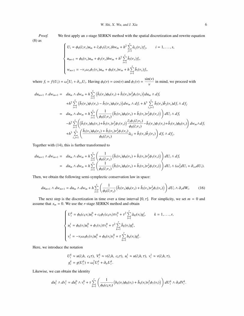
Theorem 3.3. The wave equation (8) discretized by an SPRK method in space and an SERKN method intime has a discrete multi-symplectic conservation law.

The proof is similar to that of Theorem 3.2. As an example, we use SERKN discretization in time andthe following SPRK discretization in space (which can be regarded as the Stormer-Verlet formula):

0 0 0

1 12

12

12

12︸︷︷︸

u

12

12 0

12

12 012

12︸︷︷︸

w

(22)

Proof. We first apply the SPRK method (22) to the spatial discretization for u and w respectively andobtain

Um,1 = um,Um,2 = um+1,

Wm,1 = wm +h2∂xxum,

Wm,2 = wm +h2∂xxum,

um+1 = um +h2

(Wm,1 + Wm,2),

wm+1 = wm +h2

(∂xxUm,1 + ∂xxUm,2).

(23)


Then proceed with

dum+1 ∧ dwm+1 = d(um + hwm +h2

2∂xxum) ∧ d(wm +

h2∂xxum +

h2∂xxum+1)

= dum ∧ dwm +h2

dum ∧ ∂xxdum +h2

dum+1 ∧ ∂xxdum+1

= dum ∧ dwm +h2

dUm,1 ∧ ∂xxdUm,1 +h2

dUm,2 ∧ ∂xxdUm,2

= dum ∧ dwm +h2

dUm,1 ∧ ∂xdWm,1 +h2

dUm,2 ∧ ∂xdWm,2

= dum ∧ dwm +h2

2∑i=1

(dUm,i ∧ ∂xdWm,i).

That is,

dum+1 ∧ dwm+1 − dum ∧ dwm =h2

2∑i=1

(dUm,i ∧ ∂xdWm,i). (24)

For t = tn,k, we rewrite (24) as

dun,km+1 ∧ dwn,k


m =h2

2∑i=1

(dUn,km,i ∧ ∂xdWn,k

m,i). (25)

It follows from (17) and (25) that the multi-symplectic conservation law is2∑

i=1

12

(dvn+1m,i ∧ dun+1

m,i − dvnm,i ∧ dun

m,i)h

+r∑

k=1

(1


t φ1(νt)))

(dun,km+1 ∧ dwn,k


m )τ = 0.(26)

¤Similarly, we can also obtain the following fully-discrete scheme for (8)

un,km+1 = un,k

m + hwn,km +

h2

2∂xxun,k

m ,

wn,km+1 = wn,k

m +h2

(∂xxun,km + ∂xxun,k

m+1),

Un,km = φ0(ckνt)un

m + ckφ1(ckνt)τvnm + τ2

r∑l=1

akl(νt)gn,lm , k = 1, . . . , r,

un+1m = φ0(νt)un

m + φ1(νt)τvnm + τ2

r∑k=1

bk(νt)gn,km ,

vn+1m = −νtωtφ1(νt)un

m + φ0(νt)vnm + τ

r∑k=1

bk(νt)gn,km .

(27)

4. Construction of explicit multi-symplectic schemes

Based on the general framework presented in Section 3, a large number of novel multi-symplectic schemescan be constructed. Here, an undoubted fact is that, symplectic Runge-Kutta schemes for the integrationof general Hamiltonian systems are usually implicit, and multi-symplectic integrators constructed by con-catenating symplectic Runge-Kutta methods and/or symplectic partitioned Runge-Kutta methods are usuallyimplicit. Thus, in practice, one has to solve implicit algebraic equations, often by using some iterative approx-imation methods. In this case, the resulting integration scheme may no longer be symplectic. The advantageof explicit symplectic integrators, when compared with fully implicit or partly implicit methods, is that theydo not require the solution of large and complicated systems of nonlinear algebraic or transcendental equa-tions. Therefore, it is clear that the computational cost of an implicit multi-symplectic method is usuallyhigher than that of an explicit one. Consequently, in this section, we construct two explicit multi-symplecticschemes, which are actually two multi-symplectic extended leap-frog methods. It can be observed that whenωx → 0, ωt → 0, these two new schemes Eleap-frogI and Eleap-frogII reduce to classical leap-frog schemes.


4.1. Extended leap-frog scheme I: An explicit multi-symplectic ERKN schemeIn this subsection, we pay attention to constructing an explicit 2-stage MSERKN scheme of order 2.

First of all, since ∂xxUn,km,i appear in (19), we observe that we cannot obtain un+1

m,i and vn+1m,i explicitly provided

that ∂xxUn,km,i could not be expressed explicitly. This means that, even if we use explicit SERKN methods

for both spatial and temporal discretizations, the resulting multi-symplectic scheme may not be necessarilyexplicit. We take the spatial discretization as an example. If we chose c = [0, 1]T , b1(νx) = a21(νx), andb2(νx) = a22(νx) = 0, then Un,k

m,1 = un,km , Un,k

m,2 = un,km+1, and the second and third equations in (19) become

un,km+1 =φ0(νx)un,k

m + φ1(νx)hwn,km + h2b1(νx)(ω2

xun,km + ∂xxun,k

m ),

wn,km+1 = − νxωxφ1(νx)un,k

m + φ0(νx)wn,km + hb1(νx)(ω2

xun,km + ∂xxun,k

m )

+ hb2(νx)(ω2xun,k

m+1 + ∂xxun,km+1).

From this we derive that

∂xxun,km =

un,km+1 − φ0(νx)un,k

m − φ1(νx)hwn,km

h2b1(νx)− ω2

xun,km ,

and then

∂xxun,km+1 =

un,km+2 − φ0(νx)un,k

m+1 − φ1(νx)hwn,km+1

h2b1(νx)− ω2

xun,km+1.

Then it follows that

wn,km+1 = − νxωxφ1(νx)un,k

m + φ0(νx)wn,km + hb1(νx)(ω2

xun,km + ∂xxun,k

m )

+ hb2(νx)(ω2xun,k

m+1 + ∂xxun,km+1)

= − νxωxφ1(νx)un,km + φ0(νx)wn,k

m +b1(νx)

hb1(νx)un,k

m+1 −b1(νx)hb1(νx)

φ0(νx)un,km −

b1(νx)b1(νx)

φ1(νx)wn,km

+b2(νx)hb1(νx)

un,km+2 −

b2(νx)hb1(νx)

φ0(νx)un,km+1 −

b2(νx)b1(νx)

φ1(νx)wn,km+1.

Assuming

b1(νx) =b1φ0(νx)φ1(νx)

, (28)

then we have wn,km+1 =

b2(νx)un,km+2 −

(b1(νx)ν2

xφ1(νx) + b1(νx)φ0(νx))un,k

m +(b1(νx) − b2(νx)φ0(νx)

)un,k

m+1

hb1(νx) + hb2(νx)φ1(νx).

Therefore, from (28), together with the symplectic conditions (13), (14) and order conditions of ERKNmethods proposed in [18], we can construct several 2-stage SERKN methods of order 2. In this paper, weconsider the following 2-stage SERKN methods of order 2 for the two directional discretizations, which canbe expressed in Butcher tableaus:

0 0 01 φ2(νt) 0

b(νt) φ2(νt) 0

b(νt)φ0(νt)φ2(νt)φ1(νt)

φ1(νt) − φ0(νt)φ2(νt)φ1(νt)

(29)

0 0 01 φ2(νx) 0

b(νx) φ2(νx) 0

b(νx)φ0(νx)φ2(νx)

φ1(νx)φ1(νx) − φ0(νx)φ2(νx)

φ1(νx)

(30)


where φ2(ν) =1 − φ0(ν)

ν2 .Note that as ωt → 0, ωx → 0, the above two SERKN methods (29) and (30) for time and space dis-

cretizations, respectively, reduce to the same classical 2-stage symplectic RKN (SRKN) method of order2:

0 0 0

1 12 012 012

12

This coincides with the leap-frog method

qn+1 − 2qn + qn−1

h2 = f (qn)

for problem p = f (q), q = p. The leap-frog method can be translated from the following 1-stage SRKNmethod of order 2 by exchanging the roles of p and q:

12 0

12

1

(31)

With the discretizations of the SERKN methods (29) and (30), (19) becomes the following scheme

Un,1m = un

m,

(∂xxU)n,1m =

Un,1m+1 − 2Un,1

m + Un,1m−1

2h2φ2(νx),

Un,2m = φ0(νt)un

m + φ1(νt)τvnm + τ2φ2(νt)

(ω2

t Un,1m + ∂xxUn,1

m − V′(Un,1

m )),

(∂xxU)n,2m =

Un,2m+1 − 2Un,2

m + Un,2m−1

2h2φ2(νx),

un+1m = φ0(νt)un


(ω2

t Un,1m + ∂xxUn,1

m − V′(Un,1

m )),

vn+1m = − νtωtφ1(νt)un

m + φ0(νt)vnm

+ τ(b1(νt)

(ω2

t Un,1m + ∂xxUn,1

m − V′(Un,1

m ))

+ b2(νt)(ω2

t Un,2m + ∂xxUn,2

m − V′(Un,2

m ))).

(32)

In fact, the scheme (32) gives the discretizations for (∂xxu)nm and (∂ttu)n

m by (∂xxu)nm =

unm+1 − 2un

m + unm−1

2h2φ2(νx)

and (∂ttu)nm =

un+1m − 2un

m + un−1m

2τ2φ2(νt), respectively. This also deduces an extended leap-frog scheme:

un+1m − 2un

m + un−1m

2τ2φ2(νt)=

unm+1 − 2un

m + unm−1

2h2φ2(νx)− V

′(un

m). (33)

We refer to the scheme (33) as Eleap-frogI and use this scheme to solve a linear wave equation (Problem1) in the next section. Meanwhile, the discretizations of w and v are given by

wnm+1 =

unm+2 − un

m

2hφ1(νx), vn+1

m =un+2

m − unm

2τφ1(νt).

Furthermore, we have the following theorem.


Theorem 4.1. By simply exchanging the roles of u and w in space and u and v in time, the MSERKN schemegiven by the following 1-stage SERKN methods of order 2 for the two directional discretizations can betransformed into the MSERKN scheme (33):

12 0

b(νt) φ21( νt

2 )/

2φ0( νt2 )

b(νt) φ1( νt2 )

(34)

12 0

b(νx) φ21( νx

2 )/

2φ0( νx2 )

b(νx) φ1( νx2 )

(35)

Proof. Firstly, the symplecticity of the schemes (34) and (35) can be directly obtained from Theorem3.1.

Then, we only show the details for the space discretization, and those for the time discretization aresimilar. Applying the 1-stage SERKN method (35) with the spatial discretization yields

U1 = φ0(νx

2)um +

12φ1(

νx

2)hwm,

um+1 = φ0(νx)um + φ1(νx)hwm + h2b(νx) f1,

wm+1 = −νxωxφ1(νx)um + φ0(νx)wm + hb(νx) f1,

(36)

where f1 = f (U1) = ω2xU1 + ∂xxU1. From the last two equations in (36), we get

um+1 =φ0(νx)um + φ1(νx)hwm + h2b(νx) f1

=φ0(νx)um + φ1(νx)hwm + h2b(νx)wm+1 + νxωxφ1(νx)um − φ0(νx)wm

hb(νx)

=φ0(νx)um + φ1(νx)hwm + hb(νx)b(νx)

wm+1 + ν2xb(νx)b(νx)

φ1(νx)um − hb(νx)b(νx)

φ0(νx)wm

=um + hφ1(νx)

1 + φ0(νx)(wm + wm+1).

This showsum+1 − um = h

φ1(νx)1 + φ0(νx)

(wm + wm+1). (37)

The first and last equations of (36) imply

wm+1 = − νxωxφ1(νx)um + φ0(νx)wm + hb(νx) f (U1)

= − νxωxφ1(νx)um + φ0(νx)wm + hb(νx)(ω2xU1 + ∂xxU1)

= − νxωxφ1(νx)um + φ0(νx)wm + hb(νx)(ω2

xφ0(νx

2)um + ω2

x12φ1(

νx

2)hwm + ∂xxU1

)

=wm + hφ1(νx

2)∂xxU1.

(38)

Following the approach to obtaining the leap-frog method by exchanging the roles of p and q in the SRKNmethod (31), we also exchange the roles of u and w. Then it can be deduced from the first equation of (36),(37) and (38) that

W1 = φ0(νx

2)wm +

12φ1(

νx

2)h∂xxum,

wm+1 = wm + hφ1(νx)

1 + φ0(νx)(∂xxum + ∂xxum+1),

um+1 = um + hφ1(νx

2)W1.

(39)


The first equation of (39) implies

wm+1/2 = φ0(νx

2)wm +

12φ1(

νx

2)h∂xxum = φ0(

νx

2)(

wm + hφ1(νx)

1 + φ0(νx)∂xxum

), (40)

and thenwm =

1φ0( νx

2 )wm+1/2 − h

φ1(νx)1 + φ0(νx)

∂xxum. (41)

Inserting (41) into the second equation of (39) gives

wm+1 =1

φ0( νx2 )

wm+1/2 + hφ1(νx)

1 + φ0(νx)∂xxum+1,

and furthermore,

wm =1

φ0( νx2 )

wm−1/2 + hφ1(νx)

1 + φ0(νx)∂xxum.

That is,

wm−1/2 = φ0(νx

2)(

wm − hφ1(νx)

1 + φ0(νx)∂xxum

)= φ0(

νx

2)wm − 1

2φ1(

νx

2)h∂xxum. (42)

Therefore, it follows from (40) and (42) that

wm+1/2 + wm−1/2 = 2φ0(νx

2)wm,

wm+1/2 − wm−1/2 = φ1(νx

2)h∂xxum.

(43)

On the other hand, the last equation of (39) means wm+1/2 =um+1 − um

hφ1( νx2 )

, which leads to

wm+1/2 + wm−1/2 =um+1 − um + (um − um−1)

hφ1( νx2 )

= 2φ0(νx

2)wm,

wm+1/2 − wm−1/2 =um+1 − um − (um − um−1)

hφ1( νx2 )

= φ1(νx

2)h∂xxum.

(44)

It follows from (44) that

wm =um+1 − um−1

2hφ1(νx)

(∂xxu)m =um+1 − 2um + um−1

2h2φ2(νx).

For the time discretization, it also can be proved that (∂ttu)n =un+1 − 2un + un−1

2τ2φ2(νt)and vn+1

m =un+2

m − unm

2τφ1(νt)holds. ¤

4.2. Extended leap-frog scheme II: An explicit multi-symplectic ERKN-PRK scheme

In this subsection, we construct another explicit multi-symplectic scheme based on Theorem 3.3. Weapply the SPRK method (22) to the space discretization, which is equivalent to the Stormer-Verlet that givesthe second order central difference of ∂xxUn,k

m , and apply the explicit 2-stage SERKN method (29) to the time


discretization. Then the multi-symplectic scheme (27) becomes

Un,1m = un

m,

(∂xxU)n,1m =

Un,1m+1 − 2Un,1

m + Un,1m−1

h2 ,

Un,2m = φ0(νt)un


(ω2

t Un,1m + ∂xxUn,1

m − V′(Un,1

m )),

(∂xxU)n,2m =

Un,2m+1 − 2Un,2

m + Un,2m−1

h2 ,

un+1m = φ0(νt)un


(ω2

t Un,1m + ∂xxUn,1

m − V′(Un,1

m )),

vn+1m = − νtωtφ1(νt)un

m + φ0(νt)vnm

+ τ(b1(νt)

(ω2

t Un,1m + ∂xxUn,1

m − V′(Un,1

m ))

+ b2(νt)(ω2

t Un,2m + ∂xxUn,2

m − V′(Un,2

m ))).

(45)

Just like the situation of the scheme Eleap-frogI, it can be observed that this scheme is equivalent to thefollowing form

un+1m − 2un

m + un−1m

2τ2φ2(νt)=

unm+1 − 2un

m + unm−1

h2 − V′(un

m), (46)

and the discretizations of w and v are

wnm+1 =

unm+2 − un

m

2h, vn+1

m =un+2

m − unm

2τφ1(νt).

It is also equivalent to the concatenation of the 1-stage SERKN method (34) of order 2 and SPRK method(22) applied to the temporal and spatial discretizations, respectively.

We refer to the above scheme (46) as Eleap-frogII, and in the next section, we use this scheme to solve anonlinear wave equation (Problem 2).

4.3. Analysis of linear stabilityIn this subsection, we pay attention to another significant aspect for those schemes proposed in this paper,

namely, the stability. It is known that the attractiveness of explicit schemes relies on the computationalefficiency, but such efficiency is always at the cost of stability. Although an application of the linear stabilityanalysis to nonlinear equations cannot be justified, it is found to be effective in numerical experiments. Usingthe well-known Fourier method [40], we give some linear stability analysis for the explicit multi-symplecticEleap-frogI scheme, and the stability for scheme Eleap-frogII can be analyzed in the similar way.

Set

unm = un expiξmh, vn

m = vn expiξmh,Un,1

m = Un,1 expiξmh, Un,2m = Un,2 expiξmh, etc.,

where ξ ∈ R and i =√−1. Then, substituting the above expressions into scheme (32) with V

′(Un,i

m ) = Un,im ,

we get

Un,1 = un,

Un,2 = φ0(νt)un + φ1(νt)τvn + τ2φ2(νt)(ω2

t +(eiξh − 2 + e−iξh)

2h2φ2(νx)− 1

)Un,1,

un+1 = Un,2,

vn+1 = −νtωtφ1(νt)un + φ0(νt)vn

+τ

(b1(νt)

(ω2


2h2φ2(νx)− 1

)Un,1 + b2(νt)

(ω2


2h2φ2(νx)− 1

)Un,2

).

Eliminating Un,1, Un,2, we obtain (un+1

vn+1

)= G

(un

vn

),


where

G =

1 − τ2φ2(νt) +τ2φ2(νt)θh2φ2(νx)

φ1(νt)τ

G21 1 − τ2φ2(νt) +τ2φ2(νt)θh2φ2(νx)

,

with θ = (cos ξh − 1), and

G21 =τφ1(νt)θ + τ3b2(νt)ν2

t φ2(νt)θ(ω2t − 2)

h2φ2(νx)+τ3b2φ2(νt)θ2

h4φ22(νx)

− φ1(νt)τ + b2(νt)φ2(νt)τ3(1 − ω2t ).

We can easily verify that G11G22 −G12G21 = 1. Hence, the eigenvalues of G = G(ξ, θ, νx, νt) satisfy

λ2 − (G11 + G22)λ + (G11G22 −G12G21) = 0.

That is,λ2 − (G11 + G22)λ + 1 = 0. (47)

Obviously, the roots λi (i = 1, 2) of equation (47) satisfy |λi| ≤ 1 if and only if |G11 + G22| ≤ 2. Then themethod satisfies the von Neumann condition, which is necessary for the stability [40].

Assuming |G11 + G22| ≤ 2 that∣∣∣∣1 − τ2φ2(νt) +

τ2φ2(νt)θh2φ2(νx)

∣∣∣∣ ≤ 1,

which is equivalent to

−1 ≤ 1 − τ2φ2(νt) +τ2φ2(νt)θh2φ2(νx)

≤ 1. (48)

Denote r =τ

h, and suppose 0 < r ≤ α and 0 < νt ≤ νx ≤ π

2. Since φ2(ν) is a monotonically decreasing

function on the interval [0,π

2] with φ2(0) =

12

and −2 ≤ θ ≤ 0, we obtain

12− 2α2 1/2

φ2(π/2)< 1 − τ2φ2(νt) +


< 1.

Obviously, if 0 < α ≤√

6π, then

12− 2α2 1/2

φ2(π/2)≥ −1, and the inequality (48) is satisfied.

Furthermore, it also gives a sufficient condition for the stability of Eleap-frogI. In fact, conditions 0 <

α ≤√

6π

and νt ≤ νx ≤ π

2make −1 < 1 − τ2φ2(νt) +


< 1, which implies that the equation (47) has

two distinct conjugate roots λi with |λi| = 1, i = 1, 2. Therefore, the method is linearly stable if

0 < α ≤√

6π

(or equivalently, 0 < r ≤√

6π

) and 0 < νt ≤ νx ≤ π

2.

5. Numerical experiments

5.1. The conservation laws and the solution

To investigate the performance of our explicit multi-symplectic schemes, we simulate the evolution of twowave equations as numerical experiments. All computations are done over space region [−L/2, L/2] and wealways assume the periodic boundary condition u(−L/2, t) = u(L/2, t) to exclude the boundary effects. Thelong-time conservation properties of the present schemes are examined by calculating the discrete local/totalenergy conservation laws.


The local energy conservation law of the Hamiltonian PDE (2) is (5), and for the wave equation (8), wehave

E(z) =12

(v2 + w2) + V(u), F(z) = −vw.

Integrating (5) over the (m, n)-cell gives∫ xm+1

xm

∫ tn+1

tn(∂E∂t

+∂F∂x

)dtdx = 0,

which implies∫ xm+1

xm

(E(z(x, tn+1)

) − E(z(x, tn)

))dx +

∫ tn+1

tn

(F

(z(xm+1, t)) − F(z(xm, t)

))dt = 0. (49)

For the MSERKN methods, we approximate the above integral (49) by

(Ele)mn = hs∑

i=1

(1


xφ1(νx)))

(En+1m,i − En

m,i)

+ τ

r∑

k=1

(1


t φ1(νt)))

(Fn,km+1 − Fn,k

m ),

whereEn

m,i =12((vn

m,i)2 + (wn

m,i)2) + V(un

m,i), Fn,km = −vn,k

m wn,km .

We use (E∗le)mn =(Ele)mn

τhto denote the discretization error of the local energy conservation law (5), and

(Ele)n = maxm|(E∗le)mn| to denote the error of the local energy conservation law depending on the time-step.

Then, it can be deduced from (49) that

ddtε(t) =

ddt

∫ L/2

−L/2E(x, t)dx = 0,

which means that the global energy ε(t) is a constant. Let the discrete global energy at some fixed time-steptn be

εnL = h

∑m

s∑

i=1

(1


xφ1(νx)))

Enm,i,

which is an approximation to the integral

ε(tn) =

∫ L/2

−L/2E(x, tn)dx.

The error of total energy at time tn is denoted by (Ege)n = εnL − ε0

L, where ε0L is the initial energy.

An example of multi-Hamiltonian PDE is provided by the equation

utt = uxx − χ sin u, (50)

To show the efficiency and robustness of our new schemes, in our numerical experiments, we use thefollowing schemes:

• leap-frog: the multi-symplectic leap-frog scheme (see [3])

un+1m − 2un

m + un−1m

τ2 =un

m+1 − 2unm + un

m−1

h2 − V′(un

m).

• Eleap-frogI: the multi-symplectic scheme Eleap-frogI constructed in Section 4.


• Eleap-frogII: the multi-symplectic scheme Eleap-frogII constructed in Section 4.

We note that these three schemes are explicit, conditionally stable, and of order two in both space andtime. We also note that all the three multi-symplectic schemes have the same computational cost with thesame step-sizes in time and space.

Since the second order methods Eleap-frogI and Eleap-frogII are the concatenation of two one-stage (ortwo-stage with FSAL property) symplectic methods, the computational cost of other second order explicitmulti-symplectic methods is no less than that of method Eleap-frogI or Eleap-frogII.

Problem 1. We first consider the linear wave equation

utt = uxx, (51)

for χ = 0 in (50). The initial conditions employed are

u(x, 0) = sin(πx), v(x, 0) = −19

sin(πx).

We know that the analytic solution of this problem is

u = sin(πx) cos(πt) − 19π

sin(πx) sin(πt).

Since this problem has oscillations in both space and time, method Eleap-frogI is used to compare withmethod leap-frog. In the experiment, we chose τ = 0.01, h = 0.02, L = 2, time interval [0, 20], and ωt = ωx =

π.

Numerical Results:From Figure 1, it can be seen that Eleap-frogI scheme displays a remarkable superiority over the leap-

frog scheme. Both schemes show accumulations of global errors and reasonable oscillation. The accuracy ofleap-frog scheme only reaches the magnitude of 10−3, whereas for our scheme Eleap-frogI, the error is about10−14.

Figure 2 shows the numerical error of local energy conservation law as a function of the time-step calcu-lated by (Ele)n. As can be seen, the error does not grow with time. The error obtained by leap-frog schemereaches the magnitude of 10−2 and that by Eleap-frogI scheme is about 10−3.

The numerical results related to the variation of the error of the global energy conservation law, i.e.,(Ege)n, are listed in Figure 3. For both methods, the errors do not show numerical amplifications. Eleap-frogIscheme conserves the global energy perfectly (the scale of 10−14), whereas the leap-frog scheme can onlypreserve the global energy in the scale of 10−3.

0 5 10 15 20

−18

−16

−14

−12

−10

−8

−6

−4

−2

t

log 10

(err

or)

leap−frogEleap−frogI

Figure 1: (Problem 1) The logarithm of maximum errors of solution as a function of the time-step.

Problem 2. Let the potential function V(u) in (8) be V(u) = − cos(u), which gives the well-known sine-Gordon equation with χ = 1 in (50):

utt = uxx − sin(u).


0 5 10 15 20−4

−3.5

−3

−2.5

−2

−1.5

tlo

g 10(E

le) n


Figure 2: (Problem 1) The logarithm of numerical errors of local energy conservation law as a function of the time-step.

0 5 10 15 20

−18

−16

−14

−12

−10

−8

−6

−4

−2

t

log 10

|(E

ge) n|


Figure 3: (Problem 1) The logarithm of absolute numerical errors of global energy conservation law as a function of the time-step.

We only consider the so-called breather-solution [11]

u(x, t) = 4 tan−1

( √1 − ω2

ω

cosωt

cosh(x√

1 − ω2)

).

The initial conditions are given by

u(x, 0) = 4 tan−1

( √1 − ω2

ω

1

cosh(x√

1 − ω2)

), v(x, 0) =

∂

∂t

4 tan−1

( √1 − ω2

ω

cosωt

cosh(x√

1 − ω2)

)

t=0

,

where ω = 0.95. On an infinite domain, this is a bump shaped solution which oscillates up and down withperiod 2π/ω. In the experiment, we use τ = 0.01, h = 0.02, and time interval [0, 30]. To exclude boundaryeffects, we use period boundary conditions with L = 80.

Noticing the exact solution (Figure 7) of the problem, it can be observed that there is only one wave inspatial direction. If we use the Eleap-frogI method, we have to choose νx = 0, and then the Eleap-frogImethod reduces to the Eleap-frogII method. Thus, we only need to use the Eleap-frogII discretization withfitted frequency ωt = ω = 0.95.

Numerical results:Figure 4 shows the global errors of the two methods. Both schemes display accumulations of global errors

and reasonable oscillations. The accuracy of leap-frog scheme reaches the magnitude of 10−4 and that of ourscheme Eleap-frogII is of 10−5. This is better than classical leap-frog methods.

From Figures 5 and 6, it can be concluded that the scheme Eleap-frogII has a better behavior than theleap-frog scheme in both the error of the local energy conservation law and the global energy conservationlaw. Here, the difference images between the exact solution and the numerical solutions of the leap-frog andEleap-frogII schemes are plotted in Figure 8.


0 10 20 30−8

−7

−6

−5

−4

−3

tlo

g 10(e

rror

)

leap−frogEleap−frogII

Figure 4: (Problem 2) The logarithm of maximum errors of solution as a function of the time-step.

0 10 20 30−9

−8

−7

−6

−5

−4

t

log 10

(Ele

) n


Figure 5: (Problem 2) The logarithm of numerical errors of local energy conservation law as a function of the time-step.

0 10 20 30−12

−10

−8

−6

−4

t

log 10

|(E

ge) n|


Figure 6: (Problem 2) The logarithm of absolute numerical errors of global energy conservation law as a function of the time-step.

Figure 7: (Problem 2) The exact solution of sine-Gordon equation


Figure 8: (Problem 2) The difference images between the exact solution and numerical solutions.

It is noted that Hairer and Lubich propose a long-time energy conservation scheme [41]:

yn+1 = cos(hω)yn + ω−1 sin(hω)y′n +12

h2Ψ fn,

y′n+1 = −ω sin(hω)yn + cos(hω)y′n +12

h(Ψ0 fn + Ψ1 fn+1),

where Ψ = ψ(hω), Φ = φ(hω), ψ(ξ) = sinc2(ξ), φ(ξ) = 1, fn = f (Φyn), Ψ0 = ψ0(hω), and Ψ1 = ψ1(hω).Actually, together with the symmetric conditions ψ(ξ) = sinc(ξ)ψ1(ξ) and ψ0(ξ) = cos(ξ)ψ1(ξ), this

scheme can be regarded as an ERKN method, which can be written in Butcher tableau as follows:

0 0 01 1

2φ21 0

b 12φ

21 0

b 12φ0φ1

12φ1

This scheme is not symplectic in general. However, it is symplectic in the one-dimensional cases, and theconcatenation in two directions also deduces a multi-symplectic method. For our experiments, if we usethe above scheme instead of the SERKN method (we denote the two schemes as MSHLI and MSHLII,respectively), similar results can be obtained and the numerical effects are very close to those by our newmethods constructed in this paper. The results are shown in Tables 1 and 2, where (Eu)n = max

m|un

m − unm|

represents the maximum error of the schemes at each time-step tn, and unm denotes the exact solution at (xm, tn).

τ, h scheme maxn

(Eu)n maxn

(Ele)n maxn

(Ege)n

τ = 0.01, h = 0.02 Eleap-frogI 4.974e − 14 5.741e − 3 4.530e − 14MSHLI 1.587e − 13 2.290e − 2 5.156e − 13

Table 1: Numerical results for Problem 1 of schemes Eleap-frogI and MSHLI

τ, h scheme maxn

(Eu)n maxn

(Ele)n maxn

(Ege)n

τ = 0.01, h = 0.02 Eleap-frogII 1.442e − 5 6.553e − 6 1.088e − 5MSHLII 1.382e − 5 6.720e − 6 1.101e − 5

Table 2: Numerical results for Problem 2 of schemes Eleap-frogII and MSHLII

Moreover, the two schemes MSHLI and MSHLII are also extended leap-frog schemes. Such schemescan be written as:

un+1m − (

2φ0(νt) + ν2t φ

21(νt)

)un

m + un−1m

τ2φ21(νt)

=un

m+1 −(2φ0(νx) + ν2

xφ21(νx)

)un

m + unm−1

h2φ21(νx)

− V′(un

m), (52)


with discretizations wnm+1 =

unm+2 − un

m

2hφ1(νx), vn+1

m =un+2

m − unm

2τφ1(νt), and

un+1m − (

2φ0(νt) + ν2t φ

21(νt)

)un

m + un−1m

τ2φ21(νt)

=un

m+1 − 2unm + un

m−1

h2 − V′(un

m), (53)

with discretizations wnm+1 =

unm+2 − un

m

2h, vn+1

m =un+2

m − unm

2τφ1(νt), respectively.

5.2. Dispersion analysisIn the study of wave motions, the dispersion relation and group velocity are fundamental concepts (see

[42]). A superposition of modes with different wave numbers is wave packet and the dispersion relation givesthe relationship between the wave number and the frequency of the modes. Errors in the phase and groupvelocities lead to the modes traveling with an incorrect speed, which can destroy the qualitative features ofthe solution [43]. Recent research shows that the multi-symplectic Preissman box scheme, a member of theGauss-Legendre Runge-Kutta (GLRK) family, qualitatively preserves the dispersion relation of any hyper-bolic system (see [44]). Furthermore, for linear PDEs, Frank, et al. [45] shows that the discrete dispersionrelation for general s-stage GLRK methods is monotonic and the sign of the analytic group velocity can bepreserved. In this subsection, we study the numerical dispersion relation of the schemes Eleap-frogI andEleap-frogII for linear systems.

From the perspective of integrable nonlinear PDEs, e.g., the sine-Gordon or the KdV equations, thedispersion relation of the associated linearized equation is of importance.

The general oscillatory solution to a linear PDE can be expressed in the form of

u(x, t) =

∫ ∞

−∞A(k)ei

(kx−ω(k)t

)dk, (54)

where k, ω(k), and A(k) are the wave number, wave frequency, and amplitude, respectively, and Aei(kx−ωt)

itself is a solution of the linear PDE. The wave number k and frequency ω(k) are related by the followingdispersion relation [45]:

D(ω, k) = 0⇔ ω = ω(k),

which is uniquely determined by the specified PDE and is used to characterize the system. For example, thelinearization

utt − uxx + χu = 0 (55)

of the sine-Gordon equation (50) at u = 0 has a dispersion relation

D(ω, k) = ω2 − k2 − χ = 0. (56)

The phase velocity is defined by vp(k) = ω/k. In a non-dispersive system, such as the wave equation(51), every wave has the same phase velocity (vp = c0) and the solution for t > 0 is just the initial conditiontranslated through space: u(x, t) = u(x − c0t, 0).

An important quantity of dispersive systems is the group velocity defined by, vg(k) = ω′(k) = −∂D

∂k

/∂D∂ω

.The group velocity is usually a function of the wave number k and characterizes the speed of energy transportin wave packets. In this case, ω

′′(k) , 0, and waves with different wave numbers travel with different phase

velocities vp, which brings the group velocity dispersion (GVD) and ultimately causes the spatial spreadingof the wave packet.

The dispersive properties of the discretizations can be studied by calculating their numerical dispersionrelations. To do so, we start with the discretizations of the linearized sine-Gordon equation (55) associatedwith the Eleap-frogI and Eleap-frogII schemes in their single equation format

Eleap − frogI :D2

t un−1m

2φ2(νt)− D2

xunm−1

2φ2(νx)+ χun

m = 0,

Eleap − frogII :D2

t un−1m

2φ2(νt)− D2

xunm−1 + χun

m = 0,(57)


where Dtunm =

un+1m − un

m

τand Dxun

m =un

m+1 − unm

hare the finite difference operators.

Assume a discrete general solution to a linear PDE of the form∑K

Aei(Km−Ωn), K = kh, Ω = ωτ, where

each mode is a solution provided K and Ω satisfy a numerical dispersion relation

DN(Ω,K) = 0.

For the equation (57), the corresponding numerical dispersion relations are given by

Eleap − frogI :( √

2φ2(νt)φ2(νt)τ

sinΩ

2

)2

−( √

2φ2(νx)φ2(νx)h

sinK2

)2

− χ = 0,

Eleap − frogII :( √

2φ2(νt)φ2(νt)τ

sinΩ

2

)2

−(

2h

sinK2

)2

− χ = 0.(58)

Both these two schemes preserve the form of the analytical dispersion relation (56). The exact relationship isgiven by the following theorem.

Theorem 5.1. The multi-symplectic schemes (58) qualitatively preserves the dispersion relation of the linearPDE. Specifically, there exist diffeomorphisms ψ1 and ψ2 satisfying the exact dispersion relationship

DN(Ω,K) = D(ψ1(Ω), ψ2(K)

)= ψ2

1 − ψ22 − χ = 0, (59)

where

Eleap − frogI :(ψ1(Ω), ψ2(K)

)=

( √2φ2(νt)φ2(νt)τ

sinΩ

2,

√2φ2(νx)φ2(νx)h

sinK2

),

Eleap − frogII :(ψ1(Ω), ψ2(K)

)=

( √2φ2(νt)φ2(νt)τ

sinΩ

2,

2h

sinK2

),

(60)

for −π < K,Ω < π.

Solving the numerical dispersion relations (58) gives

Eleap − frogI : Ω(K) = ±2 arcsin

√φ2(νt)r2

φ2(νx)sin2 K

2+φ2(νt)hr

2χ,

Eleap − frogII : Ω(K) = ±2 arcsin

√2φ2(νt)r2 sin2 K

2+φ2(νt)hr

2χ.

The significance of Theorem 5.1 for the non-dispersive equation (55) (with χ = 0) can be seen in Figures9–11, which show the dispersion curves Ω(K), the group velocity Ω

′(K), the group velocity dispersion Ω

′′(K)

for the exact (56), and numerical (58). In the experiment, two different values of the ratio r = τ/h, withh = 0.01 are used. The exact relation is given by Ω(K) = ±rK.

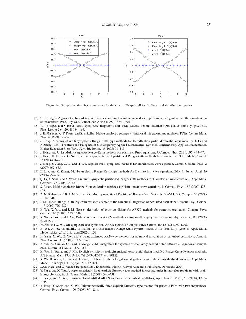
The significance of Theorem 5.1 for the linearized sine-Gordon equation (55) (with χ = 1) can be seen inFigures 12–14. The exact relation is given by Ω(K) = ±r

√K2 + h2.

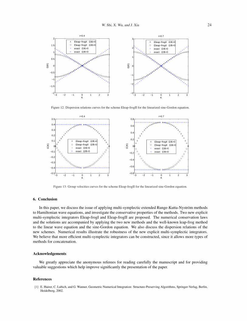
From Figures 9–14, we can see that the existence of diffeomorphisms (60) is not enough to preserve thequalitative features of the analytical solution. All of the schemes introduce numerical dispersions. From Fig-ures 10 and 13, because Ω(K) and K both have direction, we can see that the dispersion relation curves areall monotonically increasing at rates given by their numerical group velocities. Similarly, Figures 11 and 14display that the group velocity curves (see Figures 10 and 13 ) are monotonically decreasing. Therefore, con-sidering the numerical solutions of the linear wave equations given by Eleap-frogI and Eleap-frogII schemes,we further obtain the following corollaries.

Corollary 5.1. The numerical group velocities Vg(k) = Ω′(K) = −∂DN

∂K

/∂DN

∂Ωat (K,Ω) of the two schemes

Eleap-frogI and Eleap-frogII have the same sign as the group velocity vg(k) = ω′(k) = −∂D

∂k

/∂D∂ω

for theassociated pair (k, ω).

Corollary 5.2. Both Eleap-frogI and Eleap-frogII schemes introduce negative dispersion, and when the wavenumber is increasing, the numerical group velocities are monotonically decreasing.


−3 −2 −1 0 1 2 3−1.5

−1

−0.5

0

0.5

1

1.5

K

Ω(K

)

r=0.4

Eleap−frogI Ω⋅K>0Eleap−frogI Ω⋅K<0exact Ω⋅K>0exact Ω⋅K<0

−3 −2 −1 0 1 2 3

−3

−2

−1

0

1

2

3

K

Ω(K

)

r=0.7


Figure 9: Dispersion relations curves for the scheme Eleap-frogI for the linear wave equation utt = uxx.

−3 −2 −1 0 1 2 3−0.5

−0.4

−0.3

−0.2

−0.1

0

0.1

0.2

0.3

0.4

0.5

K

Ω’ (K

)

r=0.4


−3 −2 −1 0 1 2 3−0.8

−0.6

−0.4

−0.2

0

0.2

0.4

0.6

0.8

K

Ω’ (K

)r=0.7


Figure 10: Group velocities curves for the scheme Eleap-frogI for the linear wave equation utt = uxx.

−3 −2 −1 0 1 2 3

−0.3

−0.2

−0.1

0

0.1

0.2

0.3

K

Ω" (K

)

r=0.4

Eleap−frogI Ω’(K)⋅K>0

Eleap−frogI Ω’(K)⋅K<0exact

−3 −2 −1 0 1 2 3−0.5

−0.4

−0.3

−0.2

−0.1

0

0.1

0.2

0.3

0.4

0.5

K

Ω" (K

)

r=0.7

Eleap−frogI Ω’(K)⋅K>0

Eleap−frogI Ω’(K)⋅K<0exact

Figure 11: Group velocities dispersion curves for the scheme Eleap-frogI for the linear wave equation utt = uxx.


−3 −2 −1 0 1 2 3−2

−1.5

−1

−0.5

0

0.5

1

1.5

2

K

Ω(K

)

r=0.4

Eleap−frogII Ω⋅K>0Eleap−frogII Ω⋅K<0exact Ω⋅K>0exact Ω⋅K<0

−3 −2 −1 0 1 2 3−3

−2

−1

0

1

2

3

K

Ω(K

)

r=0.7


Figure 12: Dispersion relations curves for the scheme Eleap-frogII for the linearized sine-Gordon equation.

−3 −2 −1 0 1 2 3−0.5

−0.4

−0.3

−0.2

−0.1

0

0.1

0.2

0.3

0.4

0.5

K

Ω’ (K

)

r=0.4


−3 −2 −1 0 1 2 3−0.8

−0.6

−0.4

−0.2

0

0.2

0.4

0.6

0.8

K

Ω’ (K

)

r=0.7


Figure 13: Group velocities curves for the scheme Eleap-frogII for the linearized sine-Gordon equation.

6. Conclusion

In this paper, we discuss the issue of applying multi-symplectic extended Runge-Kutta-Nystrom methodsto Hamiltonian wave equations, and investigate the conservative properties of the methods. Two new explicitmulti-symplectic integrators Eleap-frogI and Eleap-frogII are proposed. The numerical conservation lawsand the solutions are accompanied by applying the two new methods and the well-known leap-frog methodto the linear wave equation and the sine-Gordon equation. We also discuss the dispersion relations of thenew schemes. Numerical results illustrate the robustness of the new explicit multi-symplectic integrators.We believe that more efficient multi-symplectic integrators can be constructed, since it allows more types ofmethods for concatenation.

Acknowledgements

We greatly appreciate the anonymous referees for reading carefully the manuscript and for providingvaluable suggestions which help improve significantly the presentation of the paper.

References

[1] E. Hairer, C. Lubich, and G. Wanner, Geometric Numerical Integration: Structure-Preserving Algorithms, Springer-Verlag, Berlin,Heidelberg, 2002.


−3 −2 −1 0 1 2 3−0.5

−0.4

−0.3

−0.2

−0.1

0

0.1

0.2

0.3

0.4

0.5

K

Ω" (K

)

r=0.4

Eleap−frogII Ω’(K)⋅K>0

Eleap−frogII Ω’(K)⋅K<0

exact Ω’(K)⋅K>0

exact Ω’(K)⋅K<0

−3 −2 −1 0 1 2 3−0.8

−0.6

−0.4

−0.2

0

0.2

0.4

0.6

0.8

K

Ω" (K

)

r=0.7

Eleap−frogII Ω’(K)⋅K>0

Eleap−frogII Ω’(K)⋅K<0

exact Ω’(K)⋅K>0

exact Ω’(K)⋅K<0

Figure 14: Group velocities dispersion curves for the scheme Eleap-frogII for the linearized sine-Gordon equation.

[2] T. J. Bridges, A geometric formulation of the conservation of wave action and its implications for signature and the classificationof instabilities, Proc. Roy. Soc. London Ser. A 453 (1997) 1365–1395.

[3] T. J. Bridges, and S. Reich, Multi-symplectic integrators: Numerical schemes for Hamiltonian PDEs that conserve symplecticity,Phys. Lett. A 284 (2001) 184–193.

[4] J. E. Marsden, G. P. Patric, and S. Shkoller, Multi-symplectic geometry, variational integrators, and nonlinear PDEs, Comm. Math.Phys. 4 (1999) 351–395.

[5] J. Hong, A survey of multi-symplectic Runge-Kutta type methods for Hamiltonlian partial differential equations, in: T. Li andP. Zhang (Eds.), Frontiers and Prospects of Contemporary Applied Mathematics, Series in Contemporary Applied Mathematics,Higher Education Press,Word Scientific Beijing, 6 (2005) 71–113.

[6] J. Hong, and C. Li, Multi-symplectic Runge-Kutta methods for nonlinear Dirac equations, J. Comput. Phys. 211 (2006) 448–472.[7] J. Hong, H. Liu, and G. Sun, The multi-symplecticity of partitioned Runge-Kutta methods for Hamiltonian PDEs, Math. Comput.

75 (2006) 167–181.[8] J. Hong, S. Jiang, C. Li, and H. Liu, Explicit multi-symplectic methods for Hamiltonian wave equation, Comm. Comput. Phys. 2

(2007) 662–683.[9] H. Liu, and K. Zhang, Multi-symplectic Runge-Kutta-type methods for Hamiltonian wave equations, IMA J. Numer. Anal. 26

(2006) 252–271.[10] Q. Li, Y. Song, and Y. Wang, On multi-symplectic partitioned Runge-Kutta methods for Hamiltonian wave equations, Appl. Math.

Comput. 177 (2006) 36–43.[11] S. Reich, Multi-symplectic Runge-Kutta collcation methods for Hamiltonian wave equations, J. Comput. Phys. 157 (2000) 473–

499.[12] B. N. Ryland, and R. I. Mclachlan, On Multisymplectic of Partitioned Runge-Kutta Methods. SIAM J. Sci. Comput. 30 (2008)

1318–1340.[13] J. M. Franco, Runge-Kutta-Nystrom methods adapted to the numerical integration of perturbed oscillators, Comput. Phys. Comm.

147 (2002) 770–787.[14] X. Wu, X. You, and J. Li, Note on derivation of order conditions for ARKN methods for perturbed oscillators, Comput. Phys.

Comm., 180 (2009) 1545–1549.[15] X. Wu, X. You, and J. Xia, Order conditions for ARKN methods solving oscillatory systems, Comput. Phys. Comm., 180 (2009)

2250–2257.[16] W. Shi, and X. Wu, On symplectic and symmetric ARKN methods, Comput. Phys. Comm. 183 (2012) 1250–1258.[17] X. Wu, A note on stability of multidimensional adapted Runge-Kutta-Nystrom methods for oscillatory systems, Appl. Math.

Modell.,doi.org/10.1016/j.apm.2012.01.053.[18] H. Yang, X. Wu, X. You, and Y. Fang, Extended RKN-type methods for numerical integration of perturbed oscillators, Comput.

Phys. Comm. 180 (2009) 1777–1794.[19] X. Wu, X. You, W. Shi, and B. Wang, ERKN integrators for systems of oscillatory second-order differential equations, Comput.

Phys. Comm. 181 (2010) 1873–1887.[20] X. Wu, B. Wang, and J. Xia, Explicit symplectic multidimensional exponential fitting modified Runge-Kutta-Nystrom methods,

BIT Numer. Math. DOI 10.1007/s10543-012-0379-z (2012).[21] X. Wu, B. Wang, K. Liu, and H. Zhao, ERKN methods for long-term integration of multidimensional orbital problems Appl. Math.

Modell., doi.org/10.1016/j.apm.2012.05.021.[22] L.Gr. Ixaru, and G. Vanden Bergehe (Eds), Exponential Fitting, Kluwer Academic Publishers, Dordrecht, 2004.[23] Y. Fang, and X. Wu, A trigonometrically fitted explicit Numerov-type method for second-order initial value problems with oscil-

lating solutions, Appl. Numer. Math., 58 (2008), 341–351.[24] H. Yang, and X. Wu, Trigonometrically-fitted ARKN methods for perturbed oscillators, Appl. Numer. Math., 58 (2008), 1375–

1395.[25] Y. Fang, Y. Song, and X. Wu, Trigonometrically fitted explicit Numerov-type method for periodic IVPs with two frequencies,

Comput. Phys. Comm., 179 (2008), 801–811.


[26] T. Monovasilis, and T.E. Simos, New second-order exponentially and trigonometrically fitted symplectic integrators for the nu-merical solution of the time-independent Schrodinger equation, J. Math. Chem, 42 (2007) 535–545.

[27] T. E. Simos, Closed Newton-Cotes Trigonometrically-Fitted Formulae of High-Order for Long-Time Integration of Orbital Prob-lems, Appl. Math. Lett. 22 (2009) 1616–1621.

[28] T. E. Simos, Closed Newton-Cotes Trigonometrically-Fitted Formulae for the Solution of the Schrodinger Equation, MATCHCommun. Math. Comput. Chem. 60 (2008) 787–801.

[29] T. E. Simos, Closed Newton-Cotes trigonometrically-fitted formulae of high order for the numerical integration of the Schrodingerequation, J. Math. Chem. 44 (2008) 483–499.

[30] T. E. Simos, High-order closed Newton-Cotes trigonometrically-fitted formulae for long-time integration of orbital problems,Comput. Phys. Commun. 178 (2008) 199–207.

[31] T. Monovasilis, Z. Kalogiratou, and T.E. Simos, Computation of the eigenvalues of the Schrodinger equation by symplectic andtrigonometrically fitted symplectic partitioned Runge-Kutta methods, Phys. Lett. A 372 (2008) 569–573.

[32] Z. Kalogiratou, Th. Monovasilis, and T.E. Simos, New modified Runge-Kutta-Nystrom methods for the numerical integration ofthe Schrodinger equation, Comput. Math. Appl. 60 (2010) 1639–1647.

[33] A. B. Gonzalez, P. Martın, and J. M. Farto, A new family of Runge-Kutta type methods for the numerical integration of perturbedoscillators, Numer. Math. 82 (1999) 635–646.

[34] T. J. Bridges, Multi-symplectic structures and wave propagation, Math. Proc. Camb. Phil. Soc. 121 (1997) 147–190.[35] R. I. McLachlan, Symplectic integration of Hamiltonian wave equations, Numer. Math. 66 (1994) 465–492.[36] K. W. Morton and D. F. Mayers, Numerical Solution of Partial Differential Equations, Cambridge University Press, 2005.[37] X. Wu, B. Wang, and J. Xia, Extended symplectic Runge-Kutta-Nystrom integrators for separable Hamiltonian systems, in Pro-

ceedings of the 2010 International Conference on Computational and Mathematical Methods in Science and Engineering, Vol. III(Editor J. Vigo Aguiar), Spain, (2010) 1016–1020.

[38] E. Hairer, S. P. Nøsett, and G. Wanner, Solving Ordinary Differential Equation I: Nonstiff Problems, Second Edition, Springer-Verlag, Berlin, Heidelberg, 1993.

[39] Y. B. Suris, On the canonicity of mappings that can be generated by methods of Runge-Kutta type for integrating systerms x′′

=

−∂U∂x

, in Russian, Zh. Vychisl. Mat. Fiz. 29 (1989), 202–211; U.S.S.R. Comput. Math. and Math. Phys. (translation), 29 (1990)138–144.

[40] A. Iserles, A First Course in the Numerical Analysis of Differential Equations, Cambridge University Press, Cambridge, 1996.[41] E. Hairer, and C. Lubich, Long-Time Energy Conservation of Numerical Methods for Oscillatory Differential Equations, SIAM

Journal on Numerical Analysis, Vol. 38, No. 2 (2001) 414–441.[42] C. M. Schober, and T. H. Wlodarczyk, Dispersive properties of multi-symplectic integrators, J. Comput. Phys. 227 (2008) 5090–

5104.[43] L. N. Trefethen, Group velocities in finite difference schemes, SIAM Rev. 24 (1982) 113–136.[44] U. M. Asher and R. I. McLachlan, Multisymplectic box scheme and the Kortweg-de Vries equation, Appl. Numer. Math. 48 (2004)

255–269.[45] J. Frank, B. E. Moore, and S. Reich, Linear PDEs and numerical methods that preserve a multisymplectic conservation law, SIAM

J. Sci. Comput. 28 (2006) 260–277.

Explicit Multi-Symplectic Extended Leap-frog Methods …xiaj/work/MSERKN.pdf · Explicit...

Documents

Transcript of Explicit Multi-Symplectic Extended Leap-frog Methods …xiaj/work/MSERKN.pdf · Explicit...