Journal of Economic Dynamics and Control 17 (1993) 327-353. North-Holland

Competition, collusion, and chaos

Donald C. Keenan University of Georgia, Arhrm, GA 30602, USA

Mike J. O’Brien Sprint, Burlingame, CA 94010, USA

Received October 1990. final version received March 1992

In this paper, we present results which show that cartel formation can still be observed in a completely deterministic model where myopic firms compete through price in finite time. The firms are spatially differentiated and take turns with their neighboring firms in setting prices. Among the different possible dynamic scenarios, we focus attention on those where cooperative and competitive behavior continue to coexist throughout time. The continual interaction of cooperative and competitive behavior results in complex dynamic regimes. Because the set of prices which firms choose will be discrete, a formal equivalence is established between the model’s dynamics and the theory of cellular automata.

1. Introduction

It is widely recognized that collusive behavior can arise in a repeated non- cooperative game from the strategic interactions of patient firms with long, usually infinite planning horizons. While similar results can be obtained within a finite horizon through considerations of incomplete information [Kreps et al. (1982)], such ‘tacit collusion’ remains in general highly sensitive to the length of the planning horizon. Indeed, in the basic Bertrand model of price competition, the set of equilibria collapses to the competitive equilibrium as soon as the horizon becomes finite.

In this paper, we present results which show that, despite the maintained assumption of myopic firms, cartel formation can still be observed in a com- pletely deterministic model in which firms compete through price in finite time. The firms are spatially differentiated and take turns with their neighboring firms in setting prices. As a result of this formulation and the assumed myopia, all

Correspondence to: Donald C. Keenan, Department of Economics, University of Georgia, Athens, GA 30602. USA.

0165-1889/93/$05.00 0 1993-Elsevier Science Publishers B.V. All rights reserved

328 D.C. Kwnan and M.J. O’Brien, Comprtirion. collusion, and chaos

strategic considerations are eliminated. Nonetheless, the resulting dynamics are shown to be capable of sustaining considerable collusive activity.

Among the different possible dynamic scenarios, we focus attention on those where cooperative and competitive behavior continue to coexist throughout time. This is made possible by the spatial extent of our model, which allows local regions to follow different standards of behavior. The continual interaction of cooperative and competitive behavior results in complex dynamic regimes.’ Collusion takes the form of unstable local cartels that are limited in both duration and extent of their market, but arise continually through time. In particular, one prominent set of reactions by firms is interpreted as the unstable dynamics proposed by Edgeworth as a solution to the Bertrand paradox. A connection is made to this and the notion of Stackelberg warfare.

Because the set of prices which firms choose will be discrete, a formal equivalence is established between the model’s dynamics and the theory of cellular automata. By this means, standard analytical tools are brought to bear on the problem of dynamic oligopoly. The propensity for environments to support collusive outcomes is interpreted in terms of exact measures of ‘self-

organization’.

2. Spatial price competition

2.1. Baikground

In reviewing Cournot’s (1838) seminal analysis of a quantity-setting oligopoly, Bertrand (1883) proposed instead that firms compete through price. Like Cournot, Bertrand maintained the assumption of myopic firms. In this formula- tion, Bertrand found that the only possible equilibrium has firms charging their lowest sustainable price, thus yielding the competitive outcome. This is often considered paradoxical, since it might be expected that, with few enough firms, collusive behavior would arise instead.

Edgeworth (1897) sought to escape this paradox by evoking the possibility of capacity constraints, or of diseconomies of scale in general. The competitive outcome would then no longer be an equilibrium, since when other marginal- cost pricing firms do not cover the market, a firm has an incentive to raise its price against the residual demand. With no price equilibrium possible, Edgeworth argued that prices would instead cycle about.

It is difficult to evaluate the possibility of Edgeworth cycles in the standard Bertrand formulation. Reaction functions are not well-defined there, given that firms want to lower price below rivals by as little as possible, but that no single

’ Most other economic models known to exhibit dynamic complexity also rely on a high rate of discount. However, see the paper by Woodford (1989).

D.C. Keenan and M. J. O’Brien, Competition, collusion. and chaos 329

choice ever accomplishes this. As in the work of Maskin and Tirole (1988) this

difficulty will be prevented here by restricting attention to a discrete number of possible prices.2

2.2. The economic model

The model employed is that of a fixed number of firms equally spaced along a ring, conveniently thought of as a circular city. Consumers are located symmetrically about the city and purchase goods from their neighboring firms in response to the prices posted by these two firms. Consumers are assumed to have symmetric preferences between the goods of their two neighboring firms, so with the symmetric distribution of consumers, each firm in the city faces the identical environment3

Each firm maximizes its current profits in a completely myopic fashion, so that its pricing decision only depends on the prices posted by its immediate neighbors, with whom it shares a market on either side. In order that a reaction to neighboring prices be well-defined, it is supposed that adjacent firms alternate every other period in setting prices. Thus, one may think of the odd-numbered firms as moving in odd periods and the even ones in even periods. This device, introduced by Cyert and DeGroot (1970) is interpreted by Maskin and Tirole (1988) in terms of price rigidities resulting from short-run commitments. For the present, this asynchronicity is to be the only difference among the otherwise identical firms.

Note that the myopia we assume assures that any observed cartel activity is not being supported by the usual folk-theorem argument for repeated games, wherein short-run deviations from collusion are punished by long-run retali- ation. Instead, cartel activity will be attributable to spontaneous self-organiza- tion. in the manner to be described.

2.3. Dynamic oligopoly as a cellular automaton

Since time as well as the firms’ common set of prices will be discrete, the resulting dynamics are those of a finite cellular automaton [Wolfram (1986)].

‘In an earlier version of this paper an alternative formulation of our model is developed, where any price is allowed, but firms choose to charge only j and (?. That formulation, unlike the standard Bertrand model, has consumers who do not regard the goods of differing firms as perfect substitutes and so their demand does not change discontinuously.

3We have taken an intermediate position between the Hotelling spatial approach and the quality/characteristic approach to product differentiation. It would be possible to take a purely Hotelling approach by regarding the goods of differently located firms as perfect substitutes, except for transportation costs, and generating demand behavior from the spatial distribution of con- sumers. It would also be possible to remove all actual spatial considerations by regarding firms as being located at different quality levels of their goods. One might then want to arrange the firms along an interval, rather than a circle, but this does not greatly affect the analysis.

330 D.C. Kwnun onrl hf. J. O’Brien. Comprtirion, collusion, and ~.Imu

This follows from the fact that firms on every site have identical reactions of the form

PI+, =.f’(pf~‘>Pf+‘).

where p: is the price at time t of the firm at the ith site. Such locally determined dynamics are exactly what distinguish a cellular automaton (CA). The only CA condition formally being violated is that sites should move synchronously. However, it is sufficient to restrict attention to, say, the odd-numbered firms, and write their reduced reaction functions synchronously as

Pf+z =f‘(.f(Pf-2,P:‘X.f‘(Pf, pf+2)) = 4(pf-2, p;, pff2) 1

i odd, t odd.

The indirect effect of a firm’s past prices on those chosen by its immediate neighbors in the previous time period allows the firm’s reduced reaction func- tion to include the firm’s own past actions.

Whether in the reduced or unreduced form, the reaction functions of our model will be ‘reflection-symmetric’. That is, due to the symmetric distribution of consumers, a firm’s choice of price depends only on the two neighboring prices and not on which of the two neighboring firms is charging which price.

Notice that because strategic considerations are absent, mixed play never occurs, and so the dynamic rules are entirely deterministic. The only factor not endogenous to the model is the historically given initial price configuration.4 Despite this deterministic setup, seemingly stochastic behavior will be seen to

emerge.

3. Cellular automata

3.1. T~prs

Since our economic model is of the form of a cellular automaton, some discussion of this class of dynamic processes will prove useful.

4Because of the lagged role of commitments, historically given forms of behavior may persist through time within a particular region. [See the discussion of the role of history in Kreps and Spence (1984) or Fudenberg and Tirole (1986).] As time passes, however, a firm is indirectly influenced by the past actions of an increasing domain of firms, and thus the behavior of a particular region may be transformed through interaction with other regions. Despite the consequent sensitiv- ity to the initial price configuration, it is a common feature of cellular automata processes that a particular rule will exhibit the same qualitative behavior for all but an exceptional set of initial configurations [as discussed by Wolfram (1983) and shown by Hurley (1990)].

D.C. KLWI~~I und M. J. 0 ‘Briw. Comprrilion. collusion, und chaos 331

Cellular automata were introduced by Von Neumann (1966) in his pioneering work on self-organizing behavior. CA rules are broadly classified into four categories, according to the dynamic behavior of their reaction functions [Wolf- ram (1986) and Hurley (1990)].5 Type I rules are those that rapidly lead from a typical initial price configuration to a steady state configuration where each firm’s price is constant over time. Thus, the effect of a local perturbation in the initial price configuration completely disappears over time for a type I rule.

Type II phenomena arise when the rule sends initial configurations into price cycles. The global cycle consists of a number of neighborhoods in different regimes, each on its own subcycle. Thus, the effect of a local perturbation in the initial configuration remains localized over time in a limited neighborhood of the firms whose prices were initially changed.

Type III rules are the most common category of CA rules and those to which we devote the most attention. Within an infinite cellular automaton, that is one with an infinite line of firm sites, type III limiting behavior is aperiodic. Unlike type I and II rules, the dynamics exhibit sensitive dependence on initial condi- tions. That is, nearly identical configurations of prices will evolve over time into increasing different configurations. This occurs despite reaction functions being in general globally noninvertible mappings that over time progressively reduce the number of possible price configurations. It is this contractive property of noninvertible dynamics that allows for self-organizing behavior. As a conse- quence of this continual contraction, an attractor emerges which represents the limiting behavior implicit in any initially disordered price configuration belong- ing to the basin of that attractor. On the other hand, it is the divergence of configurations within these ‘strange’ attractors for type III dynamics that allows self-organizing structures to be complex (neither steady states nor cycles).

Rules of the remaining type IV category are somewhat rarer and do not occur for elementary cellular automata.” We do not explicitly consider this type rule further.

3.2. Statistical meusures qf‘conzp1e.u hehacior

Complex dynamics are most easily dealt with by statistical analysis, despite the previously noted fact that our oligopoly model is entirely deterministic. The

5 While Wolfram’s classification is entirely empirical, the recent analysis of Hurley provides theoretical support for the validity of the distinction between the various types of cellular automata.

‘For type IV rules, the effect of a local perturbation in an initial configuration may grow throughout time, but whether it does so and the extent to which it does so seem unpredictable. It is thought that most type IV rules are computationally irreducible, so that no more efficient means exists for determining the effect of an initial perturbation than to simulate the rule. Whether a perturbation’s effect dies off is then undecidable in the sense that there is no assured means of answering such a question in a finite number of steps. It is furthermore thought that some if not all type IV rules are capable of acting as universal computing devices, so that each would be capable of exhibiting any specific dynamic behavior.

332 D.C. Keenan and M. J. O’Brien, Competition. collusion. and chaos

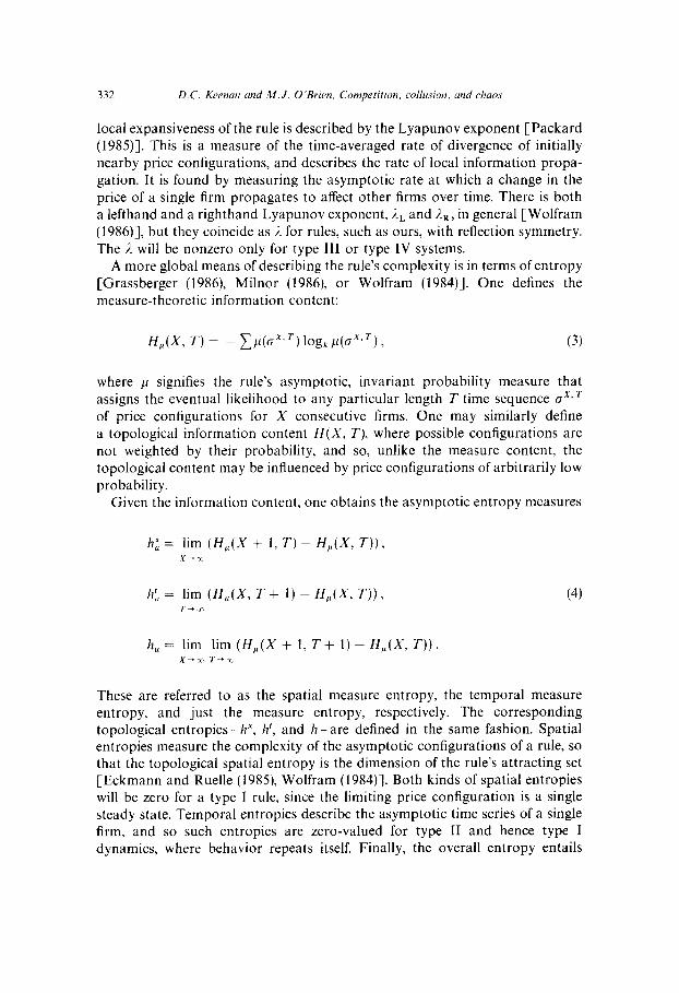
local expansiveness of the rule is described by the Lyapunov exponent [Packard (1985)]. This is a measure of the time-averaged rate of divergence of initially nearby price configurations, and describes the rate of local information propa- gation. It is found by measuring the asymptotic rate at which a change in the price of a single firm propagates to affect other firms over time. There is both a lefthand and a righthand Lyapunov exponent, iL and 2,) in general [Wolfram (1986)], but they coincide as /. for rules, such as ours, with reflection symmetry. The 1. will be nonzero only for type III or type IV systems.

A more global means of describing the rule’s complexity is in terms of entropy [Grassberger (1986), Milnor (1986), or Wolfram (1984)]. One defines the measure-theoretic information content:

H&f, 7-1 = - Cp(oXT log, p(O*,r) ) (3)

where ,U signifies the rule’s asymptotic, invariant probability measure that assigns the eventual likelihood to any particular length T time sequence c?,r of price configurations for X consecutive firms. One may similarly define a topological information content H(X, T), where possible configurations are not weighted by their probability, and so, unlike the measure content, the topological content may be influenced by price configurations of arbitrarily low probability.

Given the information content, one obtains the asymptotic entropy measures

h; = lim (H,(X + 1, T) - H,(X, T)), x-x

k: = lim (H,(X, T + 1) - H,(X, T)), T-;r

(4)

k, = lim lim (H,(X + 1, T+ 1) - H,(X, 7)). X-x T-x

These are referred to as the spatial measure entropy, the temporal measure entropy, and just the measure entropy, respectively. The corresponding topological entropies-h*, k’, and k-are defined in the same fashion. Spatial entropies measure the complexity of the asymptotic configurations of a rule, so that the topological spatial entropy is the dimension of the rule’s attracting set [Eckmann and Ruelle (1985) Wolfram (1984)]. Both kinds of spatial entropies will be zero for a type I rule, since the limiting price configuration is a single steady state. Temporal entropies describe the asymptotic time series of a single firm, and so such entropies are zero-valued for type II and hence type I dynamics, where behavior repeats itself. Finally, the overall entropy entails

D.C. Keens und M. J. O’Brien, Competiiion, collusion. and chaos 333

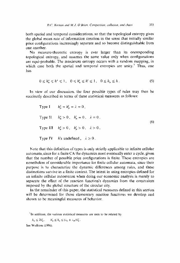
both spatial and temporal considerations, so that the topological entropy gives the global mean rate of information creation in the sense that initially similar price configurations increasingly separate and so become distinguishable from one another.

No measure-theoretic entropy is ever larger than its corresponding topological entropy, and assumes the same value only when configurations are equi-probable. The maximum entropy occurs with a random mapping, in which case both the spatial and temporal entropies are unity.7 Thus, one has

In view of our discussion, the four possible types of rules may then be succinctly described in terms of these statistical measures as follows:

Type I h; = h; = i. = 0,

Type 11 h;>O, h;=O, i=O,

(6) Type III h; > 0, h: > 0, i. > 0,

Type IV h’s undefined, i. 2 0.

Note that this definition of types is only strictly applicable to infinite cellular automata, since for a finite CA the dynamics must eventually enter a cycle, given that the number of possible price configurations is finite. These entropies are nonetheless of considerable importance for finite cellular automata, since their purpose is to characterize the dynamic differences among rules, and these distinctions survive in a finite context. The intent in using entropies defined for an infinite cellular automaton when doing our economic analysis is merely to separate the effect of the reaction function’s dynamics from the constraints imposed by the global structure of the circular city.

In the remainder of this paper, the statistical measures defined in this section will be determined for those elementary reaction functions we develop and shown to be meaningful measures of behavior.

‘In addition, the various statistical measures are seen to be related by

h, 5 2h:, hf, 5 h, s (i.,, + j.R)h;.

See Wolfram (1986).

4. Edgeworth dynamics

4.1. The role of increasing costs

In this section, we consider our framework in the simplest case of just two prices: a higher ‘cartel’ price d and a lower ‘competitive’ price @. Such a model, where each firm takes on one of but two (k = 2) states, is referred to as an elementary cellular automaton.

In addition to Bertrand-style consumers who always seek the lower price of the two firms in their neighborhood, there may also be consumers who do not regard the two firms’ goods as perfect substitutes. For definiteness, we suppose that such consumers behave exactly oppositely to the Bertrand consumers and so always purchase a fixed amount at the firm nearest to them. In contrast to this captured market, a firm gets the Bertrand consumers of one side only if its price is below that of the other firm to that side, and in the case of a tying price, the firms split the market. These two types of consumers, together with a specification of the firm’s cost function, provide sufficient flexibility to obtain the elementary CA reaction functions we consider.

An Edgeworth cycle in our context would have a firm reacting to neigh- boring low prices j by raising its price up to F. Note, however, that this may now occur entirely for demand reasons, without regard to the diseconomies of scale considered by Edgeworth. It may simply be that the revenue from charging one’s captured consumers the high price 3 exceeds getting the lower price fi from them together with half the Bertrand consumers on either side.

The other part of the Edgeworth process has the higher price d being lowered to the competitive price b, so that a price cycle is set up. Even were there only Bertrand consumers present, however, it would not follow with discrete prices that a firm need react to both its neighbors charging the cartel price $ by itself charging the competitive price p. For the case of discrete prices, the firm may prefer the higher price ; from half the Bertrand consumers together with whatever captured market it has to getting a lower price F from all the Bertrand consumers and the captured market.

Edgeworth proposed that the reaction of charging high price d when faced by low prices @ be explained by capacity constraints on the part of the rival firms. If such constraints could be present for rival firms, then they would certainly also be present for the given firm when it considers charging the low price p in reaction to the rival firms charging ;. This is, after all, the situation where this firm faces the greatest demand any firm will ever encounter. The same capacity constraints Edgeworth suggested to support the reaction d when neighboring firms both charge d also support reaction d when both neighbors charge F.

D.C. Keenan and M. J. O’Brien, Competition, collusion, and chaos 335

We examine the case where ; = f( 6, $) is indeed part of the firm’s reaction function8 This condition is obviously necessary if local high-price cartels are to arise. Further, as will now be seen, it is only with this reaction that Edgeworth economy of scale considerations need again play a role.

Given that neighboring firms both charging j? lead a firm to also charge 3, then if an Edgeworth cycle is to be set up, it is necessary that a high price ; on one side and a low price p on the other lead the firm to adopt the low price j?. This, however, can only be the case with diseconomies of scale. Indeed, if marginal cost is constant, then the assumption that neighbors both charging jj or both charging F lead the firm to charge ; logically requires that the firm also select F when neighbors charge opposite prices. This follows since, in terms of profit, the latter situation is but a convex combination of the first two situations, given that marginal costs are constant and the revenue function is additive. For the reaction function being considered to occur, the cost function must not also be additive. It must instead satisfy the condition

< tc(alP)) + m-wa) - C(ix(PlP) + f-WC)) 1 (7)

where, say, x(pIF) is the total demand from both sides for a firm charging fi when it faces firms both charging price j?. This condition requires some degree of convexity of cost, given that x is decreasing in its first argument.’

It is possible in our model for the reaction /? =f(fi, jj) to be explained entirely by demand elasticity considerations and for the reaction $ =f(b, F) to also be so explained. However, as we have seen, the only way to have both restrictions hold and yet have jj = f(b, 6), so that recurrent dynamics occur, is for increasing cost considerations to come into play. Because the reaction being discussed requires diseconomies of scale and because the rule yields unstable motion as envisioned by Edgeworth, we will refer to the reaction function

as the Edgeworth process.

‘Taking the simple quadratic cost function, one sees that the condition holds if x(6,$) - x(fi, p) > x(6. ;) - x($. J?), which one would expect to be the case. It will certainly hold for the situation with Bertrand-style as well as captured consumers, so long as their demand schedule is downward-sloping.

‘Notationally, by, say, d =f(@,;), we mean that when, say, pf-’ = p and p;+’ = b, then j f P,+, = P.

336 D.C. Keennn and M. J. O’Brien. Competition. collusion. and chaos

4.2. Obtaining Edgell,orth dynamics in the discrete price model

Rather than simply provide a parametrization for which our circular city model yields the Edgeworth process, we present a short description of the properties used to assure this outcome. Since it is sufficient for our purposes, we let the total demand .? of a firm’s captured consumers be fixed, as is the total demand .U of the Bertrand consumers to one side of a firm. We let marginal cost have the constant value c < p, up to some quantity to be discussed.”

When other firms charge j? there needs to be sufficient captured demand relative to the portion of Bertrand consumers that total demand is not very elastic going from price fi to 3. Since one obtains none of the Bertrand con- sumers when charging 3, the condition in terms of profit I7 in order that the higher price /? be chosen is that’ ’

> (9)

II(x(jljF)) = (jj - c)(< + 2).

On the other hand, when one of the rival firms charges p and the other charges J?, then one obtains half of the Bertrand consumers to one side when charging 5 and an additional half from each side when charging price $. We require that this larger portion of Bertrand consumers relative to captured demand causes total demand between J? and jj to become sufficiently elastic so that

This then assures that the lower price jj is chosen when the rival firms are charging opposite prices.

Let the marginal cost rise to C = jj near x = 2 + 3%; for definiteness, let the

rise occur exactly at this quantity. Going from the case where rival firms charge

“‘In the actual construction of reaction functions, we always have increasing costs occur as the jump at some quantity of marginal cost from a constant value c < fi to C = @. This has the advantage that a firm is always willing to absorb the demand it encounters, so that one does not need to account for spillover demand. It also helps to explain where the particular price 0 comes from.

1 ’ The reader may simply assume c = 0, so that profit comparisons become revenue comparisons. We maintain nonzero marginal cost c since in section 6 we will want to lessen costs in the lower output range in order to rationalize a second kind of reaction function.

D.C. Keenan and M. J. O’Brien, Competition, collusion, and chaos 337

opposing prices to where they both charge F, there will then be no change in profit for the given firm if it has chosen low price p, since the additional demand belongs in the high-cost range where the marginal cost coincides with price d. As a result, when the given firm instead charges high price F, the additional demand 4% that arises going from the case where neighboring firms charge opposing prices to where both charge 3 can easily prove large enough so that

n(x(;l;)) = ($ - C)(.% + X)

> (11)

despite n(ix(dld) + tx(;l~?)) < n(x(@ld)). In such a case, the firm will switch to also choosing high price $ whenever rival firms raise their prices to ;. It is here that increasing costs serve their role in limiting the profitability of dropping to the low price p when the other firms are keeping price high.

The conditions we have imposed can be satisfied for a range of parameter values of nontrivial size. Thus the Edgeworth process can be generated by our model in a robust way.

5. Analysis of Edgeworth dynamics

5.1. Injnite cellular automata

5.1. I. Formal dynamics

We consider the Edgeworth process, employing the techniques introduced to describe complex automaton rules. Using the reduction to alternate sites only, described in eq. (2), the Edgeworth process is found by a standard method of enumeration [Wolfram (1983)] to be ‘rule 90’ among elementary synchronous rules. This rule is the simplest example of a linear or additive rule, where the price reactions are specified to be the sum of the earlier neighboring states, modulus k [Martin et al. (1984)]. That is,

$tpi-2, pi,pi+2) = pi-2 + #+2 (mod 21, (12)

where in an entirely formal manner we reverse the natural labels of states, so that the cartel price is ; = 0 and the competitive price is ij = 1.

It can be shown that, for an infinite cellular automaton, additive rules act as surjective maps of configurations. This implies that all possible configurations continue to occur over time. Furthermore, configurations continue to occur

338 D.C. Keenun amI M.J. O’Brien, Competition, collusion. und clmos

with equal probability starting from a random initial configuration [Milnor (1986)]. It thus follows that

h; = hf, = 1 , (13)

with the corresponding topological entropies also being unity.” The Edgeworth rule is thus maximally chaotic both spatially and temporally, and in terms ofjust these statistics cannot be distinguished from a truly random mapping. Nonethe- less, inspection of a typical dynamic development (fig. 1) convinces one that the behavior is not truly random.’ 3

5.1.2. Curte1.c

The most prominent regularity of the Edgeworth process consists of the sequences of adjacent high-price firms that organize and persist in the fashion of a local cartel. These cartels, however, are unstable and unravel over time as competition at the fringes of the cartel cause the marginal firms to abandon the cartel. Thus, such cartels appear as triangles, as they spring up and then die off.

As we have just seen, such temporal-spatial behavior is not reflected in either the spatial or temporal entropies separately, though this lack of randomness is revealed by the Edgeworth process entropy

h,=2, (14)

which combines consideration of time and space. The topological entropy has this same value and indicates that, quite unlike a random mapping, it takes the history of but two adjacent sites to reconstruct the entire development of an infinite cellular automaton following the Edgeworth rule.

Given that it is the high-price sequences that are of interest in our analysis of cartels, we introduce some other measures that distinguish Edgeworth’s rule from random behavior. We define Q(i) as the density of high-price sequences of exact length i, so that the two firms bordering the sequence are of low price. Lind (1984) shows this distribution to be of the form

Q(i) = i(2))‘. (15)

lZIt is easily seen that the Lyapunov exponent i. for the Edgeworth process is unity, since by (12) a price change by one firm cannot help but change the prices of neighboring firms in the next period.

‘-‘Given an arbitrary initial price configuration, then, as described in the caption of fig. 1, the dynamic evolution of prices is obtained by successive application of rule 90 [eq. (12)] to each firm site.

D.C. Keenan and M. J. O’Brien, Competition, collusion, and chaos 339

Fig. 1. Edgeworth dynamics (leader-leader dynamics).

Evolution of the one-dimensional cellular automaton where alternate firms are allowed to change prices at alternate times according to Edgeworth dynamics [eq. (8)]. Firms charging the ‘competitive’ low prices p are represented as white rectangles; firms charging the ‘cartel’ high price 5 are represented as black rectangles. The configuration of the cellular automaton at successive time steps is shown on successive lines, going down the page. The prices of firms are initially uncorrelated with one another and are taken to be j or J? with probability l/2. The evolution is shown for 120 firm sites for 300 periods. Site I and 120 are treated as neighbors, producing a circular city of sites. While Edgeworth dynamics are maximally chaotic. it is nevertheless apparent that cartels persist over time (black triangles) more commonly than random chance would dictate. While an infinite chaotic cellular automaton does not cycle, the fact that a fixed number of sites (120) are used produces a cycle, as indicated by the fact that. for example, lines A and B

are identical.

As a spatial measure, this density is again identical to that of a random initial configuration, Q”(i) = (4)“‘. However, turning once more to both spatial and temporal considerations, it is clear for the Edgeworth process that the density T(i) of cartel triangles of length i is of the same basic form as Q(i), since

340 D.C. Kmwun und M. J. 0 ‘Brim, Competition, cohion, and chaos

a high-price sequence always persists over time as a triangle. More precisely, we obtain

T(i) = A(2)_‘. (16)

On the other hand, triangular configurations for random mappings must be of a far lower density, on the order of F(i) = ())pci), where p(i) is proportional to i’. (This follows since a high-price sequence at one moment of time would then indicate nothing about the next time step, and so a ‘cartel’ of i original firms is but the coincidental occurrence of high prices throughout a triangular region.) It is thus formally established that cartels persist under the Edgeworth process in a manner not accountable for by random occurrence and that this nonrandom behavior can be measured using the statistical measures of complexity we have introduced.

5.2. Finite cellulm uutomata

The preceding discussion precisely concerns infinite cellular automata, where the reaction function’s effect is isolated from that of the environment. The primary difference in the finite case is that, rather than remaining aperiodic, type III dynamics must eventually enter into cycles. Because the additivity property allows an algebraic analysis, precise results are available concerning these cycles and their transients in the case of an Edgeworth process [Martin et al. (1984)]. The upshot is that the maximum period of cycles as well as the number of these cycles grows on average exponentially with n, the number of pairs of firms. Most cycles have periods near their maximum. Transients, on the other hand, grow at most linearly with n. For all these reasons, most configurations appear on a cycle of near the maximum period. Thus, as the number of firms grows large, it becomes increasingly difficult in a set amount of time to distin- guish the finite case from the infinite aperiodic case, and the entropy measures of the infinite cellular forms become increasingly accurate descriptors of the finite case.

6. Leader-follower dynamics

While rather complete results are available for additive processes such as Edgeworth’s dynamics, additive CA are quite exceptional within the class of type III processes in that they exhibit maximum spatial entropy. Nonadditive cellular automata are almost always contractive maps that force greater self- organization than do the surjective maps of additive cellular automata. Thus,

D.C. Keenan and M.J. O’Brien, Competition. collusion, and chaos 341

with nonadditive reaction functions, cartels will arise more consistently than with the Edgeworth process.

Our framework can rationalize any number of nonadditive reactions when more than two prices are permitted, but to obtain reactions of this kind of behavior within the two-price formulation we need to relax the assumption of identical firms. The simplest way to do this is to let alternate firms differ from one another. We continue to assume that, say the odd firms, follow Edgeworth’s dynamics, but now the even ones have the reaction function

This can occur, for instance, if the even firms still face the same demand as the odd ones but their costs are less than those of Edgeworth firms at lower levels of output [less than X(J? 1 j?)]. Such a low-cost firm prefers to keep prices down, and so attract customers, in those situations where it has not reached its low-cost capacity.

6.2. The dynamics

When we look at the reduced dynamics for the odd firms,

Pf+2 =fklW23 P:,, 67(Pf, Pf+2)) 7 i odd, t odd, (18)

we find it is ‘rule 18’ among elementary cellular automata (fig. 2b). On the other hand, looking at the reduced dynamics of the even firms,

Pf+2 = sm-23 PfMPf, P:+2)) 1 i even, t even, (19)

it is found to be ‘rule 126’ (fig. 2~). Whether one examines the reduced dynamics in isolation or their conjunction

in the unreduced dynamics (fig. 2a), it is apparent that significant organization by firms into cartels is occurring. At the same time, however, forces of competi- tion are undermining the cartels, and the resulting dynamics are chaotic, rather than degenerating into either perfect competition or a global cartel (type I phenomena). This behavior is reflected in the statistical measures of rule 18 or rule 126 [Wolfram (1986)], which, as one would expect, yield identical results:

Rule 18 or 126

hz=$, hL=+, h,=l, j.=l. (20)

Entropies smaller than those of rule 90 indicate that possible configurations are being eliminated over time as the dynamics induce considerable cartel

formation. Nonetheless, these entropies do not vanish, indicating that the tension between competition and collusion persists over time.

6.3, LeaderTfdlott~er dynamics LT. leades-leuder Stackelberg ttwfure

Both the Edgeworth firms with reaction function (18) and their neighboring firms with reaction function (19) share the feature that they will support a cartel from within but will undercut it at the fringe, The Edgeworth firms differ from their neighbors in that the former will abandon a competitive regime and raise

Fig. Za. Leader-follower dynamics.

Evolution of the cellular automaton according to leader-follower dynamics: odd sites evolve according to eq. (X), even sites according to eq. (17), at alternate times. The initial configuration is identical to that used in fig. I. However. the degree of self-organization is much greater than with Edgeworth dynamics, as evidenced by the more frequent occurrence and large size of the cartels which persist over time (triangles). As in fig. I. due to its finite nature the cellular automaton has

begun cycling. as indicated by the identity of lines A and B.

D.C. Keenan and M. J. O’Brien, Competition, collusion, and chaos 343

The

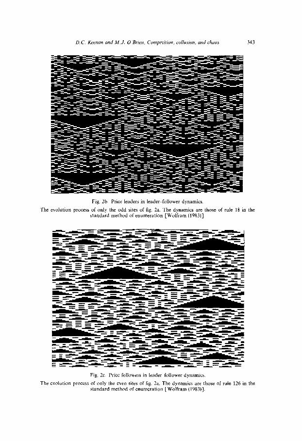
Fig. 2b. Price leaders in leader-follower dynamics.

evolution process of only the odd sites of fig. 2a. The dynamics are those of rule 18 in standard method of enumeration [Wolfram (1983)].

the

The

Fig. 2c. Price followers in leader-follower dynamics.

evolution process of only the even sites of fig. 2a. The dynamics are those of rule 126 in standard method of enumeration [Wolfram (1983)].

the

344 D.C. Keenun und M. J. O’Brien, Contpetirion. collusion, and chaos

price, whereas the latter will continue to support the competitive regime. In this sense, we refer to the Edgeworth firms as price leaders and the other firms as price followers.

With rule 90, all firms are price leaders and so it is not surprising that the outcome is maximally chaotic, in the form of Stackelberg (1934) warfare. On the other hand, when price leaders alternate with price followers (fig. 2a), then in contrast to the Stackelberg outcome, the result is one of more regular behavior, supporting extensive collusive activity.14

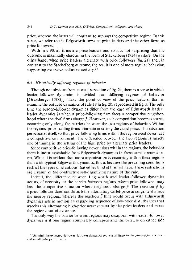
6.4. Historically d@ering regimes of behavior

Though not obvious from casual inspection of fig. 2a, there is a sense in which leader-follower dynamics is divided into differing regimes of behavior [Grassberger (1983)]. Take the point of view of the price leaders, that is, examine the reduced dynamics of rule 18 in fig. 2b, reproduced in fig. 3. The only time the leader-follower dynamics differ from the case of Edgeworth leader- leader dynamics is when a price-following firm faces a competitive neighbor- hood where the rival firms charge ii. However, such competition becomes scarce, occurring only along the barriers between the two regions of behavior. Within the regions, price-leading firms alternate in setting the cartel price. This situation perpetuates itself, so that price-following firms within the region need never face a competitive environment. The difference between the two regions is merely one of timing in the setting of the high price by alternate price leaders.

Since competitive price-following never arises within the regions, the behavior there is indistinguishable from Edgeworth dynamics in these same circumstan- ces. While it is evident that more organization is occurring within these regions than with typical Edgeworth dynamics, this is because the prevailing conditions restrict the types of situations that either kind of firm will face. These restrictions are a result of the contractive self-organizing nature of the rule.

Indeed, the difference between Edgeworth and leader-follower dynamics occurs, of necessity, at the barrier between regions, where price followers may face the competitive situation where neighbors charge @. The reaction j by a price follower does not disturb the alternating cartel-price arrangement inside the nearby regions, whereas the reaction p’ that would occur with Edgeworth dynamics sets in motion an expanding sequence of low-price disturbances that wrecks this alternating high-price arrangement by the price leaders and mixes the regions out of existence.

The only way the barrier between regions may disappear with leader-follower dynamics is if one region completely collapses and the barriers on either side

14As might be expected. follower-follower dynamics reduces all firms to the competitive low price and so all entropies to zero.

D.C. Keenan and M.J. O’Brien. Cornperition, collusion, und chaos 345

Fig. 3. Regions for price followers in leader-follower dynamics

This figure is identical to fig. 2b (i.e.. it represents evolution based on rule I#), except that in one of its two type regions rectangles corresponding to p are colored grey. This is done to show that, for rule IX evolution, it is only along the border of these two type regions that two price-following firms. both charging fi, will be neighbors. It is only when two such firms charging p are neighbors that leader-follower dynamics differ from leaderleader dynamics. The obviously more organized nature of the inside of the regions as compared to fig. 1 is solely a result of the reductton there in the number

of possible conditions faced by a firm.

annihilate one another, as occurs in the top portion of fig. 3. Such a collapse occurs only when an entire region cartelizes and then this cartel unravels under the pressure of the outside mode of behavior on either side. Only when there is a single region will its complete cartelization persist over time, in the form of a global cartel. Thus, large-scale cartelization of an entire region of behavior has an all-or-nothing aspect to it, in that the presence of any competing mode of behavior will instead result in the complete elimination of the cartelized regime. Nonetheless, the competitive outcome is even more unstable and so cartels continue to arise over time.

346 D.C. Ktwmn utd M. J. O’Brien, Conpririon. collusion, and clruos

Since barriers at each moment of time are being newly affected by the past actions of one additional firm to each side, their movement is a random walk with diffusion coefficient ) [Grassberger (1983)l.l’ Given only a finite number of firms, the wandering barriers would then tend to annihilate one another over time, so that a single pattern of behavior would emerge. This is limited only by the fact that the oligopoly may enter a price cycle before this need happen.

6.5. Dependence on new information and scale imariunce

It has been seen that while a rational firm’s reaction function must depend on neighboring firms’ previous, now fixed prices and not on its own previous, now variable price, the reduced reaction function can indeed involve the firm’s own past behavior. Nonetheless, in the case of Edgeworth dynamics, that is rule 90 [eq. (S)], it turns out that even the reduced dynamics do not depend on a firm’s own past behavior. By continuing the process of reduction, one sees that among all the firms whose past actions might be influencing a particular firm’s choice, only the outermost ones actually do. These firms’ prices constitute newly arriving relevant information.

The total dependence of the choice of price on new information and not on own past history represents an absence of inertia, which serves to explain the extreme variability and apparent randomness of Edgeworth dynamics. This complete dependence on newly arrived information shows in extreme form the distinction of type III chaotic dynamics from type I or II dynamics, where a firm’s state throughout time depends only on a limited neighborhood of firms. The newly arriving influence of increasingly distant firms allows type III dy- namics to have regions continually mix cooperative and competitive behavior, without ever completely settling into one or the other mode.

As just seen, Edgeworth dynamics appear the same for any uniformly spaced sampling of representative firms, no matter the scale. This indicates the self- similar, fractal nature [Mandelbrot (1983)] of these chaotic systems.16 For leader-follower dynamics there is still much self-similarity, though it is more

IsThe competitive low-price barrier persists until it is absorbed into a cartel containing an even number of price leaders (not to be absorbed is IO encounter a cartel of length zero). This cartel dwindles until the competitive low-price barrier reappears at its bottom. The original length of the cartel is dictated by those price leaders of the two neighboring regimes who are not of necessity charging a high price. Since these alternate price-leading firms satisfy Edgeworth dynamics, so that spatially their price configuration is random, it follows that the position of the barrier going into the cartel is random. Therefore the position at which the cartel dies and the barrier reappears is also random with respect to the barrier’s initial position. The distribution is clearly a binomial one, and so, for an infinite cellular automaton. the barrier follows a random walk.

“See the discussion of Mandelbrot (1983) in the context of cotton prices.

D.C. Keenun and M. J. O’Brien, Comprrition, collusion. and chaos 341

limited in the small due to the greater degree of local self-organization. That is, it takes an additional reduction of, say, rule 126, the price follower’s dynamics, before it appears self-similar, becoming, in fact, rule 90. Note that this invariance of scale only applies within a relevant range, limited in the small by firm size and in the large by the finiteness of the economic environment.”

7. Multiple price environments

Collusion is but one example of a standard of behavior, and interest naturally focuses on how different standards, which in our model have a regional charac- ter, can persist and interact over time. Besides cartels, we have considered the two out-of-phase regions of behavior that become apparent in the leader- follower model after a certain amount of transformation. When a firm is allowed more than two price levels, such coexistent regions of differing behavior can arise in striking fashion, which are quite apparent without having to first transform the patterns (see figs. 4 and 5).18 As the number of prices increases, however, the set of possible dynamic rules rapidly explodes in size. Therefore, the particular examples presented in this section are meant not so much to be important in and of themselves, as to display significant features characteristic of broad classes of chaotic rules when in multiple price environments.”

7.1. Stable sets

In their interpretation as standards of behavior, our dynamic regimes bear a certain resemblance to Von NeumannMorgenstern stable sets [Greenberg

“If the reductions are done on rule 18, the price leader’s dynamics. then, as indicated in earlier discussion, there will be two regions. one that appears as the Edgeworth dynamics and the other as a high-price cartel.

‘“The reaction function used to generate ftg. 4 is identical to that of fig. 1 when a is relabeled j?. with the addition of

The reaction function used to generate fig. 5 is identical to that of fig. 3 when fi is relabeled $ and d is relabeled [, with the addition of

jt;. j) = ii. .f(A fi) = $. .f(d.P)=P. (odd tirms) ,

H(E 0) = P 1 st8, P) = p, Y(D> P) = d 1 (even firms)

‘“Except for the Edgeworth cycle in reaction to the three possible combinations of two prices, all other combinations of reactions for any number of prices can be obtained from the demand side alone, when confining attention to discrete prices. Revenue values supporting the desired reactions can always be found, and upon selecting prices this gives demand values. Moreover, it is known that aggregate demand values can be arbitrary at a finite number of prices [Shafer and Sonnenschein (1982)]. Therefore, with the exception of the two-price Edgeworth cycles, whose rationalization requires nonlinearities in the cost function, any reaction function can be rationalized using the demand side only.

348 D.C. Keenun und hf. J. O’Brien, Comprtirion. collu.Mn, und chaos

(1986)]. Like stable sets, each regime consists of a set of possible configurations and there are in general several such regimes possible. Each regime displays internal stability in the sense that, beginning with a configuration within the regime, one obtains only further configurations within that regime. Furthermore. if the regime is not to be transient, they must also be externally stable in the sense that competing regimes must not collapse the given regime at its edges. While the cartels of chaotic dynamics display internal stability, they lack external stability. It is this failure that causes them to be only components of large regimes, rather than being themselves enduring standards of behavior.

If, on the other hand, there are to be several coexisting behavioral regimes, a particular pattern of conduct must not display too strong external domina- tion; that is, it must not consistently erode the neighboring regimes. This balance of power between regimes is rather delicate. Even if there is average balance, so that regions only expand and contract in an apparently random fashion, we have already seen that with sufficient time one arbitrary regime will come to dominate. Once again, however, such long-run behavior may be cut short by the cycle that must occur with a finite number of firms.

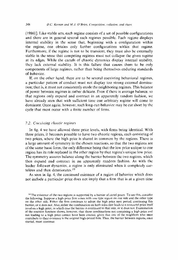
7.2. Coexisting clzuotic regimes

In fig. 4 we have allowed three price levels, with firms being identical. With three prices, it becomes possible to have two chaotic regions, each consisting of two prices, where the high price is shared in common by the regions. There is a large amount of symmetry in the chosen reactions, so that the two regions are of the same basic form, the only difference being that the low price unique to one region has its role replaced in the other region by that region’s unique low price. The symmetry assures balance along the barrier between the two regions, which then expand and contract in an apparently random fashion. As with the leader-follower dynamics, a region is only eliminated when it completely car- telizes and then deteriorates.”

As seen in fig. 4, the continued existence of a region of behavior which does not include a particular price does not imply that a firm that is at a given time

“The existence of the two regions is supported by a barrier of cartel prices. To see this, consider the following. Suppose a high-price firm arises with one type region on one side and the other type on the other side. Either the firm continues to adopt the high price next period, continuing this barrier, or it does not. Also, either the combination on both sides that leads to a noncartel price itself involves a high price, in which case the barrier is continued to that side, or it does not. Examination of the reaction function shows, however, that those combinations not containing a high price and not leading to a high price cannot have been created, given that one of the neighbors who must contribute to their existence is the original high-priced firm. Thus, the barrier between regions, once started, must continue.

D.C. Krenan nnd M. J. O’Brien, Cornpr/i/ion, collusion, und chaos 349

i-A

L B

Fig. 4. Differing chaotically collusive regimes,

This figure is the evolution for identical firms of a rule which is a combination of two different Edgeworth dynamics. The two types of Edgeworth regions have the same cartel price, but a different lower price, so that there are three prices in all. This figure illustrates the fact that the behavior of regions can be quite complex. For example, as can be seen in the upper right portion of the figure, a region can be eradicated by an opposing region which is itself eradicated at a later time by a region identical to the first one. Thts Implies that a given site can be a member of several regions at different times in the evolution, Since time periods A and B are identical. the figure exhibits a cycle having

both regions of behavior. The value of each site is initially uncorrelated and is taken as p, ii, or b with probability 13.

a member of the regime will never charge that price. This follows since the firm may at some time pass out of this regime. The persistence of a region does not imply the persistence of this standard of behavior by any particular firms, but rather that the behavior continues to be passed on to some collection of firms.

Fig. 5. Competltlvc and chaotically collusive regimes

The dynamics in this figure involve three prices and firms of alternating type. Now. white represents the intermediate priced, whereas the low price p is represented in prey. Firms act as either leaders or

followers with respect to the intermediate and high prices /? and f. This shows up as chaotic regions of the same type as fig. ?a. In addition. however. the low price p is stable. so that there are also regions of competitive behavior. While firms remain in one region or another for all time, their inclusion in any particular region is the result of the rules’ interaction with the initial conditions and not of differences in the firms themselves. The value of each site is initially uncorrelated and is taken

a5 p, J?. or $ with probability I :3.

In fig. 5 we also allow three prices, but now firms again differ from their neighbors. Thereby we can generate two regions of behavior, one of type I and one of type III.

The dynamics are those of the leader-follower type with regard to the two

higher prices 8 and ;. In the presence of the low price ,6, though, a leader will always raise the price to the greater value of his two neighbors, whereas

D.C. Keenan and M. J. O’Brien, Competition. collusion, und chaos 351

a follower will always adopt the low price. As a result, the low price is stable and so purely competitive regimes coexist with the leader-follower regimes of recurring collusive activity. Observe that the particular firms that constitute the competitive regime are fixed over time, though this results from inherited circumstances and not from any inherent behavior special to just these firms.

This figure is particularly useful for considering the effect of different size cities, since each chaotic region may be interpreted in this fashion. The only difference from a city proper is that there is a boundary of always competitive firms, rather than there being a circular city closing in on itself. As might be expected, the simulations show that narrower regimes lead to more rapid self-organization and cycling.2’

The external balance between the competitive and collusive regimes of fig. 4 is of a more subtle form than our general discussion of external stability might have indicated. The competitive price is not robust against both other prices, but it does not need to be since matters arrange themselves, due to the self-

organizing nature of the rule, so that cartelized firms charging d and the competitive firms charging J? never come into contact. They are, instead, separ- ated by a pair of firms charging the intermediate price F. Potentially price- following firms react to one neighbor charging d and the other d by themselves charging @, which provides the outer edge of the competitive regime. The adjacent, potentially price-leading firms react instead to the situation of one neighbor charging p and the other F by themselves charging d, which serves to set up the given reaction of their aforementioned competitive neighbors. Finally, these firms charging $ are in turn substantiated by their price-following neigh- bors to the other side who react to one firm charging a and the other not charging b by charging fi as well. Since the price b does not arise from the leader-follower environment on the outside, the annunciated scheme of reac- tions is self-supporting and secures a regime of competitive prices within. Thus, external stability does not require that a standard of behavior dominate all possible alternatives, but rather that on average it prevails over the alternatives that actually arise. Which alternatives actually arise can depend delicately on the overall character of the dynamics.

While all the transient cartels in our examples have been triangular, such precision is by no means necessary. With sufficient prices, cartels may grow and contract in complicated fashions. In particular, the steady decline of our triangu- lar cartels is due to their contact with a noncartel price that continually undercuts the cartel by causing fringe firms to abandon the cartel and adopt that noncartel price. Instead, a noncartel price in contact with a cartel might lead to

” Compared to a true circular city, though, this effect is attenuated by the boundary condition, which acts to continually inject newly competitive forces, rather than reflect the already processed information coming out of the other side of a self-enclosed city.

352 0.q. KW~UW stud M. J. O’Brien, Competition. collusion, and chaos

an advancing sequence of different noncartel prices at the edge of the unraveling cartel that eventually ends with the cartel price. At this point, the cartel will have ceased unraveling and will have expanded by a firm site. Depending on the price of the newly neighboring firm it then encounters, the cartel may expand further or begin another sequence of contractions. While this scenario would appear to allow for a wide variety of shapes of cartels, depending on the sequence of impinging prices, simulations show that highly organizing rules will arrange that cartels actually encounter a very small number of different sequences of prices. Typically then, after a short transient period due to the initial conditions, only a very small number of different shaped cartels will occur.

8. Conclusion

The classical Bertrand model of price competition by myopic firms does not permit collusive activity to arise. We have altered that model in a number of regards in order to weaken competitive forces. In particular, we have introduced spatial product differentiation, explicit dynamics, and increasing-cost considera- tions. On the other hand, we have maintained the assumption that firms are myopic. It is relaxation of this assumption which is typically the critical element in permitting game-theoretic explanations of collusion; so, in maintaining this assumption, it is established that the collusive activity observed in this paper is of a different nature, arising from spontaneous self-organization.

Given our changes, we have demonstrated that cartel formation can be supported by a variety of dynamic reactions obtainable from our model. We have also shown that a natural extension of Edgeworth dynamics to our model results in collusion and competition chaotically interacting throughout time. The formal analysis of the economic model has been shown to be identical to that of a cellular automaton. Measures of complex behavior developed for cellular automata have been shown to be meaningful measures of the self-organizing tendencies of our economic model. The reduction of conflict via the introduction of follower firms was reflected in the reduction of these entropy measures.

The leader-leader and leader-follower dynamics we have examined were obtained by introducing significant nonlinearity in tastes and technology. These nonlinearities are at the root of the chaotic dynamics that have been the focus of this analysis.

References

Bertrand, J., 1883, Theorie mathematique de la richesse sociale, Journal des Savanis, 499-508. Cournot, A., 1838, Recherches sur les principes mathematiques de la theorie des richesses; English

edition: N. Bacon, ed., Researches into the mathematical principles of the theory of wealth (MacMillan, New York, NY).

D.C. Keenan and M. J. O’Brien, Competition, collusion, and chaos 353

Cyert, R. and M. DeGroot, 1970, Multiperiod decision models with alternating choice as the solution of the duopoly problem, Quarterly Journal of Economics 84, 419-429.

Eckmann, J.P. and D. Ruelle, 1985, Ergodic theory of chaos and strange attractors, Review of Modern Physics 57, 617-656.

Edgeworth, F., 1897, La teoria pura de1 monopolio, Giornale degh Economisti 40, 13-31; English edition: The pure theory of monopoly, in: F. Edgeworth, ed., Papers relating to political economy, Vol. 1 (Macmillan, London).

Fudenberg, D. and J. Tirole, 1986, Dynamic models of oligopoly (Harwood, London). Crassberger, P., 1983, New mechanism for deterministic diffusion, Physical Review A 28366663667. Grassberger, P., 1986, Toward a quantitative theory of self-generated complexity, International

Journal of Theoretica! Physics 25, 907-938. Greenberg, J., 1986, Stable standards of behavior: A unifying approach to solution concepts, IMSS

technical report no. 484 (Stanford University, Stanford, CA). Hurley, M., 1990, Attractors in cellular automata, Ergodic Theory and Dynamical Systems 10,

131-140. Kreps, D. and A.M. Spence, 1984, Modelling the role of history in industrial organization and

competition, in: G. Feiwel, ed., Contemporary issues in modern microeconomics (Macmillan, London).

Kreps, D., J. Milgrom, J. Roberts, and R. Wilson, 1982, Rational cooperation in the finitely repeated prisoner’s dilemma, Journal of Economic Theory 27, 245-252.

Lind, D., 1984, Applications of ergodic theory and sofic systems to cellular automata, Physica 10 D, 36-44.

Mandelbrot, B., 1983, The fractal geometry of nature (W.H. Freeman and Co., New York, NY). Martin, O., A.M. Odlyzko, and S. Wolfram, 1984, Algebraic properties of cellular automata,

Communications in Mathematical Physics 93, 219-258; also in: Wolfram (1986). Maskin, E. and J. Tirole, 1988, A theory of dynamic oligopoly, II: Price competition, kinked demand

curves, and Edgeworth cycles, Econometrica 56, 571-599. Milnor, J., 1986, Directional entropies of cellular automaton-maps, in: E. Bienenstock, F. Fogelman

Soulie, and G. Weisbuch, eds., Disordered systems and biological organization (Springer, Berlin). Packard, N., 1985, Complexity of growing patterns in cellular automata, in: J. Demongeot, E. Gales,

and M. Tchvente, eds., Dynamical systems and cellular automata (Academic Press, New York, NY).

Shafer, W. and H. Sonnenschein, 1982, Market demand and excess demand functions, in: K.J. Arrow and M.D. Intriligator, eds., Handbook of mathematical economics, Vol. 3 (North-Holland, Amsterdam).

Von Neumann, J., 1966, Theory of self-reproducing automata, Completed and edited by A.W. Burks (University of Ihinois, Urbana-Champaign, IL).

Von Stackelberg, H., 1934, Marktform und Gleichgewicht (Julius Springer, Vienna). Wolfram, S., 1983, Statistical mechanics of cellular automata, Review of Modern Physics 55,

602-644; also in: Wolfram (1986). Wolfram, S., 1984, Universality and complexity in cellular automata, Physica 10 D, l-35; also in:

Wolfram (1986). Wolfram, S., 1986, Theory and applications of cellular automata (World Scientific, Singapore), Woodford, M., 1989, Imperfect financial intermediation and complex dynamics, in: W.A. Barnett, J.

Geweke, and K. Shell, eds., Economic complexity (Cambridge University Press, Cambridge).