0 0 M O N T H 2 0 1 7 | V O L 0 0 0 | N A T U R E | 1

LETTERdoi:10.1038/nature20780

Compensatory water effects link yearly global land CO2 sink changes to temperatureMartin Jung1, Markus Reichstein1,2, Christopher R. Schwalm3, Chris Huntingford4, Stephen Sitch5, Anders Ahlström6,7, Almut Arneth8, Gustau Camps-Valls9, Philippe Ciais10, Pierre Friedlingstein11, Fabian Gans1, Kazuhito Ichii12,13, Atul K. Jain14, Etsushi Kato15, Dario Papale16, Ben Poulter17, Botond Raduly16,18, Christian Rödenbeck19, Gianluca Tramontana16, Nicolas Viovy10, Ying-Ping Wang20, Ulrich Weber1, Sönke Zaehle1,2 & Ning Zeng21,22

Large interannual variations in the measured growth rate of atmospheric carbon dioxide (CO2) originate primarily from fluctuations in carbon uptake by land ecosystems1–3. It remains uncertain, however, to what extent temperature and water availability control the carbon balance of land ecosystems across spatial and temporal scales3–14. Here we use empirical models based on eddy covariance data15 and process-based models16,17 to investigate the effect of changes in temperature and water availability on gross primary productivity (GPP), terrestrial ecosystem respiration (TER) and net ecosystem exchange (NEE) at local and global scales. We find that water availability is the dominant driver of the local interannual variability in GPP and TER. To a lesser extent this is true also for NEE at the local scale, but when integrated globally, temporal NEE variability is mostly driven by temperature fluctuations. We suggest that this apparent paradox can be explained by two compensatory water effects. Temporal water-driven GPP and TER variations compensate locally, dampening water-driven NEE variability. Spatial water availability anomalies also compensate, leaving a dominant temperature signal in the year-to-year fluctuations of the land carbon sink. These findings help to reconcile seemingly contradictory reports regarding the importance of temperature and water in controlling the interannual variability of the terrestrial carbon balance3–6,9,11,12,14. Our study indicates that spatial climate covariation drives the global carbon cycle response.

Large interannual variations in recently measured atmospheric CO2 growth rates originate primarily from fluctuations in carbon uptake by land ecosystems, rather than from the oceans or variations in anthro-pogenic emissions1–3. There is a general consensus that the tropical regions contribute the most to terrestrial carbon variability1,8,18,19. The observed positive correlation between mean tropical land temperature and CO2 growth rate3,5,6,12,13 implies smaller land carbon uptake and enhanced atmospheric CO2 growth during warmer years, with a sensitivity of about 5 gigatonnes of carbon per year per K. There is a tight relationship between this sensitivity on interannual timescales and long-term changes in terrestrial carbon per degree of warming across multiple climate carbon-cycle models6.

Despite this strong emergent relationship with mean tropical land temperature, several studies suggest that variations in water availability

have an important8,10,11,14, even a dominant role4,9, in shaping the inter-annual variability (IAV) of the carbon balance of extensive semi-arid and sub-tropical systems. Furthermore, the recent doubling of the tropical carbon cycle sensitivity to interannual temperature variability has been linked to interactions with changing moisture regimes13. A full understanding of the processes governing the climatic controls of terrestrial carbon cycling on interannual timescales and across spatial scales is therefore still lacking. Here we show that the ‘temperature versus water’ debate can be resolved by simultaneously assessing the carbon-cycle response to fluctuations in both temperature and water availability at both local and global scales.

Using both machine learning algorithms and process-based global land models, we derived spatial and temporal patterns of the IAV of CO2 uptake by plants via photosynthesis (GPP) and of CO2 loss through respiration (TER). NEE equals TER minus GPP, thus allowing analysis of the IAV of NEE for CO2.

Machine learning algorithms were used to translate gridded inputs of daily air temperature, water availability and radiation, among others15, into time-varying 0.5° grids of TER and GPP for the 1980–2013 period (FLUXCOM; see Methods). Three machine learning algorithms were trained on FLUXNET20-based in situ TER and GPP flux estimates from two flux partitioning methods21,22. These three fitting algorithms combined with two partitioning methods provided six sets of GPP and TER estimates each, which combined yield 36 FLUXCOM NEE ensemble members.

In a complementary approach, we examined simulations of GPP and TER from an ensemble of seven global land surface or dynamic vegetation models16,17 (TRENDYv3, see Methods). These process-based model simulations follow a common protocol and used the same climate-forcing data set as the observation-based FLUXCOM models. Both sets of results are expected to be more uncertain in the tropics owing to the less reliable climate- and satellite-based inputs and a sparse coverage of flux measurements23.

We analysed FLUXCOM and TRENDYv3 simulations independently, but in a consistent manner. We derived NEE as the difference between TER and GPP, that is, a positive value of NEE indicates a flux of carbon from the land to the atmosphere. To isolate IAV we detrended GPP and TER for each grid cell and month (see Methods). We find that

1Department of Biogeochemical Integration, Max Planck Institute for Biogeochemistry, 07745 Jena, Germany. 2Michael-Stifel-Center Jena for Data-driven and Simulation Science, Friedrich- Schiller-Universität Jena, 07743 Jena, Germany. 3Woods Hole Research Center, 149 Woods Hole Road, Falmouth, Massachusetts 02540, USA. 4Centre for Ecology and Hydrology, Wallingford, Oxfordshire OX10 8BB, UK. 5College of Life and Environmental Sciences, University of Exeter, Exeter EX4 4QF, UK. 6Department of Earth System Science, School of Earth, Energy and Environmental Sciences, Stanford University, Stanford, California 94305, USA. 7Department of Physical Geography and Ecosystem Science, Lund University, 223 62 Lund, Sweden. 8Karlsruhe Institute of Technology, Institute of Meteorology and Climate Research, 82467 Garmisch-Partenkirchen, Germany. 9Image Processing Laboratory, Universitat de València, Catedrático José Beltrán, Paterna 46980, València, Spain. 10Laboratoire des Sciences du Climat et de l’Environnement, CEA CNRS UVSQ, 91191 Gif-sur-Yvette, France. 11College of Engineering, Mathematics and Physical Sciences, University of Exeter, Exeter EX4 4QE, UK. 12Department of Environment Geochemical Cycle Research, Japan Agency for Marine-Earth Science and Technology, 3173-25, Showa-machi, Kanazawa-ku, Yokohama 236-0001, Japan. 13Center for Global Environmental Research, National Institute for Environmental Studies, 16-2 Onogawa, Tsukuba, 305-8506, Japan. 14Department of Atmospheric Sciences, University of Illinois, Urbana, Illinois 61801, USA. 15Global Environment Program, The Institute of Applied Energy, Tokyo 105-0003, Japan. 16Department for Innovation in Biological, Agro-food and Forest systems, University of Tuscia, 01100 Viterbo, Italy. 17NASA Goddard Space Flight Center, Biospheric Science Laboratory, Greenbelt, Maryland 20771, USA. 18Department of Bioengineering, Sapientia Hungarian University of Transylvania, 530104 M-Ciuc, Romania. 19Max Planck Institute for Biogeochemistry, Department of Biogeochemical Systems, 07745 Jena, Germany. 20CSIRO Oceans and Atmosphere, PMB #1, Aspendale, Victoria 3195, Australia. 21Institute of Atmospheric Physics, Chinese Academy of Science, Beijing 100029, China. 22Department of Atmospheric and Oceanic Science, University of Maryland, College Park, Maryland 20742, USA.

© 2017 Macmillan Publishers Limited, part of Springer Nature. All rights reserved.

2 | N A T U R E | V O L 0 0 0 | 0 0 M O N T H 2 0 1 7

LETTERRESEARCH

FLUXCOM TRENDY

c d1980 1990 2000 2010 1980 1990 2000 2010

0 0.5 1.0 1.5 2.0 0 0.5 1.0 1.5 2.0

40

0

–40

80

1

0

–1

2

–2NE

E IA

V (n

orm

aliz

ed)

Latit

ude

(°)

R2 = 0 R2 = 0.89 R2 = 0.14 R2 = 0 R2 = 0.84 R2 = 0.19

NEE NEERAD NEETEMP NEEWAI

Mean grid-cell IAV (normalized) Mean grid-cell IAV (normalized)

a b

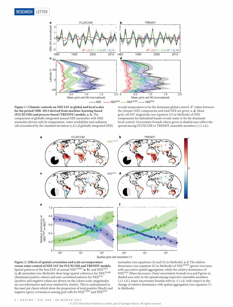
Figure 1 | Climatic controls on NEE IAV at global and local scales for the period 1980–2013 derived from machine-learning-based (FLUXCOM) and process-based (TRENDY) models. a, b, The comparison of globally integrated annual NEE anomalies with NEE anomalies driven only by temperature, water availability and radiation (all normalized by the standard deviation (s.d.) of globally integrated NEE)

reveals temperature to be the dominant global control. R2 values between the climatic NEE components and total NEE are given. c, d, Mean grid-cell IAV magnitude (see equation (3) in Methods) of NEE components for latitudinal bands reveals water to be the dominant local control. Uncertainty bounds where given as shaded area reflect the spread among FLUXCOM or TRENDY ensemble members (± 1 s.d.).

FLUXCOM TRENDY

Spatial grid-cell resolution (°)

a b

c d

e f

Rel

ativ

e d

omin

ance

of

NE

ETE

MP

or

NE

EW

AI

1.0

0.8

0.6

0.4

0.2

0100 101 102 100 101 102

NEETEMP

NEEWAI

+

0

–

Figure 2 | Effects of spatial covariation and scale on temperature versus water control of NEE IAV for FLUXCOM and TRENDY models. Spatial patterns of the first EOF of annual NEETEMP (a, b), and NEEWAI (c, d) anomalies (see Methods) show large spatial coherence for NEETEMP (dominant positive values) and anti-correlated patterns for NEEWAI (positive and negative values are shown on the colour scale; magnitudes are not informative and were omitted for clarity). This is underpinned in the inset pie charts which show the proportion of total positive (black) and negative (grey) covariances among grid cells for NEETEMP and NEEWAI

anomalies (see equations (4) and (5) in Methods). e, f, The relative dominance (see equation (6) in Methods) of NEETEMP (green) increases with successive spatial aggregation, while the relative dominance of NEEWAI (blue) decreases. Outer uncertainty bounds in e and f given as shaded area refer to the spread among respective ensemble members (± 1 s.d.); inner uncertainty bounds refer to ± 1 s.d. with respect to the change of relative dominance with spatial aggregation (see equation (7) in Methods).

© 2017 Macmillan Publishers Limited, part of Springer Nature. All rights reserved.

0 0 M O N T H 2 0 1 7 | V O L 0 0 0 | N A T U R E | 3

LETTER RESEARCH

global patterns of NEE IAV are consistent between FLUXCOM and TRENDYv3 (Extended Data Fig. 1 and Supplementary Information section 1). Both approaches reproduce (r ≈ 0.8) the globally integrated NEE IAV derived from atmospheric CO2 concentration measurements and transport24. Both approaches also show the largest IAV in the tropics (Extended Data Fig. 1). To obtain the contributions of different environmental variables to IAV, we decomposed carbon flux anomalies (Δ FLUX) of each year, month, and grid cell (subscripts y, m and s) into their additive components forced by detrended anomalies of temperature (Δ TEMP), shortwave incoming radiation (Δ RAD), and soil-moisture-related water availability (Δ WAI; see Methods):

ε

Δ = ×Δ + ×Δ

+ ×Δ +

Δ ≈Δ +Δ +Δ

a a

a

FLUX TEMP RAD

WAI

FLUX FLUX FLUX FLUX

(1)s,m,y s,m

TEMPs,m,y s,m

RADs,m,y

s,mWAI

s,m,y s,m,y

s,m,y s,m,yTEMP

s,m,yRAD

s,m,yWAI

Here as,m represents the estimated sensitivity of the flux anomaly, ΔFLUXs,m,y (GPP or TER) to each respective climate-forcing anomaly (Δ TEMP, Δ RAD, Δ WAI) for a given grid cell and month, and εs,m,y is the residual error term. The product of a given sensitivity (for example, aTEMP) and corresponding climate-forcing anomaly (for example, Δ TEMP) constitutes the flux anomaly component driven by this climate factor (for example, GPPTEMP). Thus, equation (1) estimates the contributions of temperature, radiation, and water availability anomalies to the carbon flux anomalies (see Supplementary Information section 2 for verification).

Our analysis reveals a contrasting pattern of NEE IAV controlled by temperature or moisture, depending on spatial scale. At the global scale, temperature drives spatially integrated NEE IAV (Fig. 1a and b, compare green and black curves), in line with previous findings based on correlations between anomalies in temperature and CO2 growth rate3,5,6,12,13. Globally integrated NEE anomalies due to variations in radiation (NEERAD) and water availability (NEEWAI) play only a minor part (compare red, blue and black curves in Fig. 1a and b). The domi-nant global influence of temperature is in contrast to the dominant local influence of water availability when analysing all grid cells indi-vidually (Fig. 1c and d; compare blue and black curves of zonal mean of grid-cell IAV).

Radiation causes the smallest NEE IAV at the grid-cell level (red curve in Fig. 1c and d) but there are indications based on other climate-forcing data that radiation could have a more important role than temperature locally (Supplementary Information section 3). Temperature variations are important for NEE IAV (green curve in Fig. 1c and d) in high latitudes and the inner tropics, but in general, the grid-cell average water-related NEE variability (NEEWAI, blue curve) is larger. Water-related NEE variability peaks at subtropical latitudes where semi-arid ecosystems dominate. This finding is consistent with studies emphasizing the role of water-limited semi-arid ecosystems on global NEE IAV4,9. We now assess how this can be reconciled with the emergent temperature control of globally integrated NEE IAV. Going from grid-cell to global scale shifts the emerging controls on NEE IAV from water availability (local) towards temperature (global).

NEE

Mean grid-cell IAV (normalized)0 1 2 0 1 2

50

0

–50

c dTER

FLUXCOM TRENDYa bGPP

50

0

–50

50

0

–50

e f

Latit

ude

(°)

WAITEMP

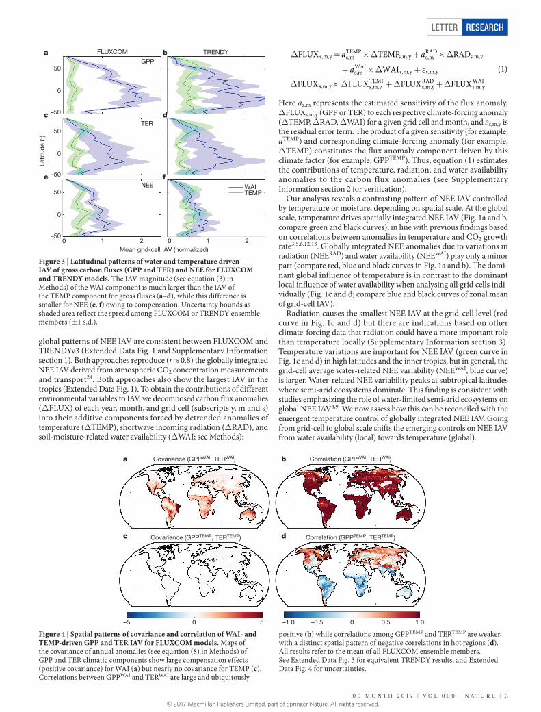
Figure 3 | Latitudinal patterns of water and temperature driven IAV of gross carbon fluxes (GPP and TER) and NEE for FLUXCOM and TRENDY models. The IAV magnitude (see equation (3) in Methods) of the WAI component is much larger than the IAV of the TEMP component for gross fluxes (a–d), while this difference is smaller for NEE (e, f) owing to compensation. Uncertainty bounds as shaded area reflect the spread among FLUXCOM or TRENDY ensemble members (± 1 s.d.).

a b

c d

Covariance (GPPWAI, TERWAI) Correlation (GPPWAI, TERWAI)

Covariance (GPPTEMP, TERTEMP) Correlation (GPPTEMP, TERTEMP)

–5 0 5 –1.0 0 1.0–0.5 0.5

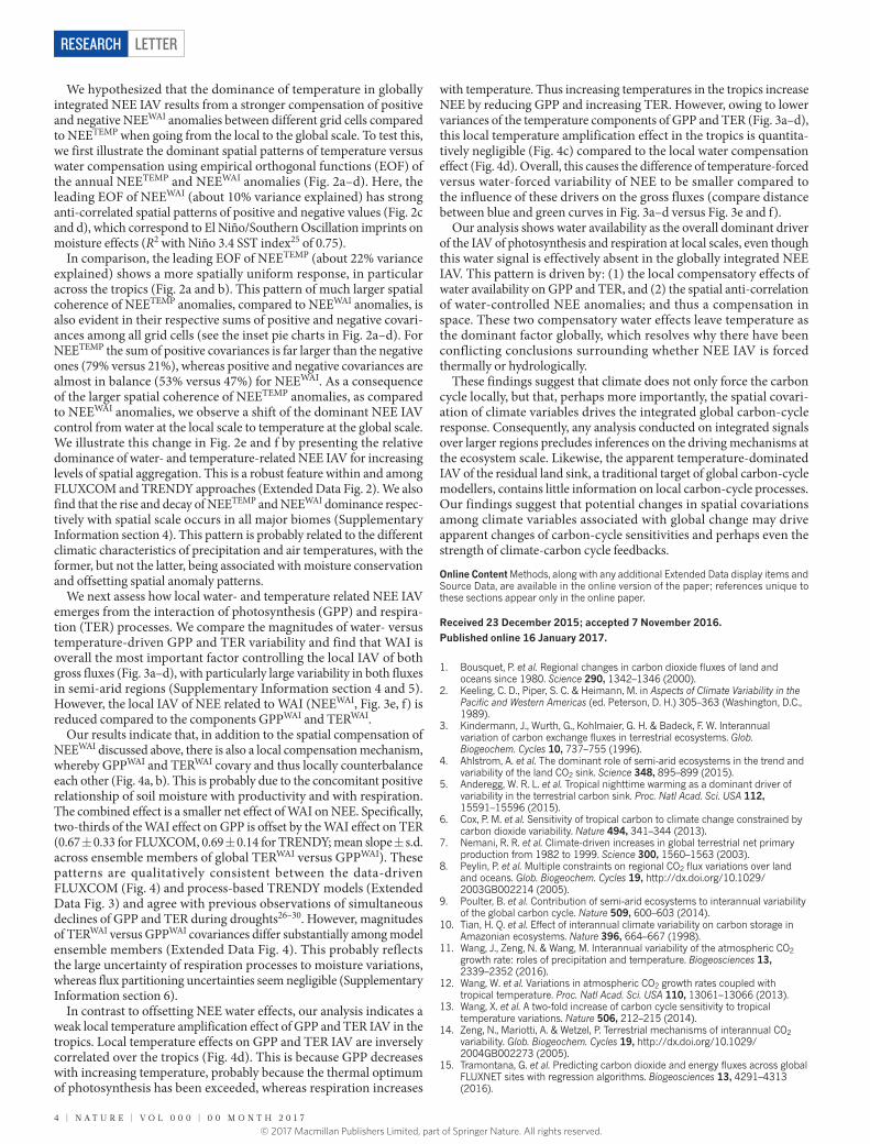
Figure 4 | Spatial patterns of covariance and correlation of WAI- and TEMP-driven GPP and TER IAV for FLUXCOM models. Maps of the covariance of annual anomalies (see equation (8) in Methods) of GPP and TER climatic components show large compensation effects (positive covariance) for WAI (a) but nearly no covariance for TEMP (c). Correlations between GPPWAI and TERWAI are large and ubiquitously

positive (b) while correlations among GPPTEMP and TERTEMP are weaker, with a distinct spatial pattern of negative correlations in hot regions (d). All results refer to the mean of all FLUXCOM ensemble members. See Extended Data Fig. 3 for equivalent TRENDY results, and Extended Data Fig. 4 for uncertainties.

© 2017 Macmillan Publishers Limited, part of Springer Nature. All rights reserved.

4 | N A T U R E | V O L 0 0 0 | 0 0 M O N T H 2 0 1 7

LETTERRESEARCH

We hypothesized that the dominance of temperature in globally integrated NEE IAV results from a stronger compensation of positive and negative NEEWAI anomalies between different grid cells compared to NEETEMP when going from the local to the global scale. To test this, we first illustrate the dominant spatial patterns of temperature versus water compensation using empirical orthogonal functions (EOF) of the annual NEETEMP and NEEWAI anomalies (Fig. 2a–d). Here, the leading EOF of NEEWAI (about 10% variance explained) has strong anti-correlated spatial patterns of positive and negative values (Fig. 2c and d), which correspond to El Niño/Southern Oscillation imprints on moisture effects (R2 with Niño 3.4 SST index25 of 0.75).

In comparison, the leading EOF of NEETEMP (about 22% variance explained) shows a more spatially uniform response, in particular across the tropics (Fig. 2a and b). This pattern of much larger spatial coherence of NEETEMP anomalies, compared to NEEWAI anomalies, is also evident in their respective sums of positive and negative covari-ances among all grid cells (see the inset pie charts in Fig. 2a–d). For NEETEMP the sum of positive covariances is far larger than the negative ones (79% versus 21%), whereas positive and negative covariances are almost in balance (53% versus 47%) for NEEWAI. As a consequence of the larger spatial coherence of NEETEMP anomalies, as compared to NEEWAI anomalies, we observe a shift of the dominant NEE IAV control from water at the local scale to temperature at the global scale. We illustrate this change in Fig. 2e and f by presenting the relative dominance of water- and temperature-related NEE IAV for increasing levels of spatial aggregation. This is a robust feature within and among FLUXCOM and TRENDY approaches (Extended Data Fig. 2). We also find that the rise and decay of NEETEMP and NEEWAI dominance respec-tively with spatial scale occurs in all major biomes (Supplementary Information section 4). This pattern is probably related to the different climatic characteristics of precipitation and air temperatures, with the former, but not the latter, being associated with moisture conservation and offsetting spatial anomaly patterns.

We next assess how local water- and temperature related NEE IAV emerges from the interaction of photosynthesis (GPP) and respira-tion (TER) processes. We compare the magnitudes of water- versus temperature-driven GPP and TER variability and find that WAI is overall the most important factor controlling the local IAV of both gross fluxes (Fig. 3a–d), with particularly large variability in both fluxes in semi-arid regions (Supplementary Information section 4 and 5). However, the local IAV of NEE related to WAI (NEEWAI, Fig. 3e, f) is reduced compared to the components GPPWAI and TERWAI.

Our results indicate that, in addition to the spatial compensation of NEEWAI discussed above, there is also a local compensation mechanism, whereby GPPWAI and TERWAI covary and thus locally counterbalance each other (Fig. 4a, b). This is probably due to the concomitant positive relationship of soil moisture with productivity and with respiration. The combined effect is a smaller net effect of WAI on NEE. Specifically, two-thirds of the WAI effect on GPP is offset by the WAI effect on TER (0.67 ± 0.33 for FLUXCOM, 0.69 ± 0.14 for TRENDY; mean slope ± s.d. across ensemble members of global TERWAI versus GPPWAI). These patterns are qualitatively consistent between the data-driven FLUXCOM (Fig. 4) and process-based TRENDY models (Extended Data Fig. 3) and agree with previous observations of simultaneous declines of GPP and TER during droughts26–30. However, magnitudes of TERWAI versus GPPWAI covariances differ substantially among model ensemble members (Extended Data Fig. 4). This probably reflects the large uncertainty of respiration processes to moisture variations, whereas flux partitioning uncertainties seem negligible (Supplementary Information section 6).

In contrast to offsetting NEE water effects, our analysis indicates a weak local temperature amplification effect of GPP and TER IAV in the tropics. Local temperature effects on GPP and TER IAV are inversely correlated over the tropics (Fig. 4d). This is because GPP decreases with increasing temperature, probably because the thermal optimum of photosynthesis has been exceeded, whereas respiration increases

with temperature. Thus increasing temperatures in the tropics increase NEE by reducing GPP and increasing TER. However, owing to lower variances of the temperature components of GPP and TER (Fig. 3a–d), this local temperature amplification effect in the tropics is quantita-tively negligible (Fig. 4c) compared to the local water compensation effect (Fig. 4d). Overall, this causes the difference of temperature-forced versus water-forced variability of NEE to be smaller compared to the influence of these drivers on the gross fluxes (compare distance between blue and green curves in Fig. 3a–d versus Fig. 3e and f).

Our analysis shows water availability as the overall dominant driver of the IAV of photosynthesis and respiration at local scales, even though this water signal is effectively absent in the globally integrated NEE IAV. This pattern is driven by: (1) the local compensatory effects of water availability on GPP and TER, and (2) the spatial anti- correlation of water-controlled NEE anomalies; and thus a compensation in space. These two compensatory water effects leave temperature as the dominant factor globally, which resolves why there have been conflicting conclusions surrounding whether NEE IAV is forced thermally or hydrologically.

These findings suggest that climate does not only force the carbon cycle locally, but that, perhaps more importantly, the spatial covari-ation of climate variables drives the integrated global carbon-cycle response. Consequently, any analysis conducted on integrated signals over larger regions precludes inferences on the driving mechanisms at the ecosystem scale. Likewise, the apparent temperature-dominated IAV of the residual land sink, a traditional target of global carbon-cycle modellers, contains little information on local carbon-cycle processes. Our findings suggest that potential changes in spatial covariations among climate variables associated with global change may drive apparent changes of carbon-cycle sensitivities and perhaps even the strength of climate-carbon cycle feedbacks.

Online Content Methods, along with any additional Extended Data display items and Source Data, are available in the online version of the paper; references unique to these sections appear only in the online paper.

Received 23 December 2015; accepted 7 November 2016.

Published online 16 January 2017.

1. Bousquet, P. et al. Regional changes in carbon dioxide fluxes of land and oceans since 1980. Science 290, 1342–1346 (2000).

2. Keeling, C. D., Piper, S. C. & Heimann, M. in Aspects of Climate Variability in the Pacific and Western Americas (ed. Peterson, D. H.) 305–363 (Washington, D.C., 1989).

3. Kindermann, J., Wurth, G., Kohlmaier, G. H. & Badeck, F. W. Interannual variation of carbon exchange fluxes in terrestrial ecosystems. Glob. Biogeochem. Cycles 10, 737–755 (1996).

4. Ahlstrom, A. et al. The dominant role of semi-arid ecosystems in the trend and variability of the land CO2 sink. Science 348, 895–899 (2015).

5. Anderegg, W. R. L. et al. Tropical nighttime warming as a dominant driver of variability in the terrestrial carbon sink. Proc. Natl Acad. Sci. USA 112, 15591–15596 (2015).

6. Cox, P. M. et al. Sensitivity of tropical carbon to climate change constrained by carbon dioxide variability. Nature 494, 341–344 (2013).

7. Nemani, R. R. et al. Climate-driven increases in global terrestrial net primary production from 1982 to 1999. Science 300, 1560–1563 (2003).

8. Peylin, P. et al. Multiple constraints on regional CO2 flux variations over land and oceans. Glob. Biogeochem. Cycles 19, http://dx.doi.org/10.1029/ 2003GB002214 (2005).

9. Poulter, B. et al. Contribution of semi-arid ecosystems to interannual variability of the global carbon cycle. Nature 509, 600–603 (2014).

10. Tian, H. Q. et al. Effect of interannual climate variability on carbon storage in Amazonian ecosystems. Nature 396, 664–667 (1998).

11. Wang, J., Zeng, N. & Wang, M. Interannual variability of the atmospheric CO2 growth rate: roles of precipitation and temperature. Biogeosciences 13, 2339–2352 (2016).

12. Wang, W. et al. Variations in atmospheric CO2 growth rates coupled with tropical temperature. Proc. Natl Acad. Sci. USA 110, 13061–13066 (2013).

13. Wang, X. et al. A two-fold increase of carbon cycle sensitivity to tropical temperature variations. Nature 506, 212–215 (2014).

14. Zeng, N., Mariotti, A. & Wetzel, P. Terrestrial mechanisms of interannual CO2 variability. Glob. Biogeochem. Cycles 19, http://dx.doi.org/10.1029/ 2004GB002273 (2005).

15. Tramontana, G. et al. Predicting carbon dioxide and energy fluxes across global FLUXNET sites with regression algorithms. Biogeosciences 13, 4291–4313 (2016).

© 2017 Macmillan Publishers Limited, part of Springer Nature. All rights reserved.

0 0 M O N T H 2 0 1 7 | V O L 0 0 0 | N A T U R E | 5

LETTER RESEARCH

16. Le Quéré, C. et al. Global carbon budget 2014. Earth Syst. Sci. Data Discuss. 7, 521–610 (2014).

17. Sitch, S. et al. Recent trends and drivers of regional sources and sinks of carbon dioxide. Biogeosciences 12, 653–679 (2015).

18. Gurney, K. R., Baker, D., Rayner, P. & Denning, S. Interannual variations in continental-scale net carbon exchange and sensitivity to observing networks estimated from atmospheric CO2 inversions for the period 1980 to 2005. Glob. Biogeochem. Cycles 22, http://dx.doi.org/10.1029/2007gb003082 (2008).

19. Peylin, P. et al. Global atmospheric carbon budget: results from an ensemble of atmospheric CO2 inversions. Biogeosciences 10, 6699–6720 (2013).

20. Baldocchi, D. Turner Review No. 15. ‘Breathing’ of the terrestrial biosphere: lessons learned from a global network of carbon dioxide flux measurement systems. Aust. J. Bot. 56, 1–26 (2008).

21. Lasslop, G. et al. Separation of net ecosystem exchange into assimilation and respiration using a light response curve approach: critical issues and global evaluation. Glob. Change Biol. 16, 187–208 (2010).

22. Reichstein, M. et al. On the separation of net ecosystem exchange into assimilation and ecosystem respiration: review and improved algorithm. Glob. Change Biol. 11, 1424–1439 (2005).

23. Schimel, D. et al. Observing terrestrial ecosystems and the carbon cycle from space. Glob. Change Biol. 21, 1762–1776 (2015).

24. Rödenbeck, C., Houweling, S., Gloor, M. & Heimann, M. CO2 flux history 1982–2001 inferred from atmospheric data using a global inversion of atmospheric transport. Atmos. Chem. Phys. 3, 1919–1964 (2003).

25. Rayner, N. A. et al. Global analyses of sea surface temperature, sea ice, and night marine air temperature since the late nineteenth century. J. Geophys. Res. D 108, http://dx.doi.org/10.1029/2002JD002670 (2003).

26. Biederman, J. A. et al. Terrestrial carbon balance in a drier world: the effects of water availability in southwestern North America. Glob. Change Biol. 22, 1867–1879 (2016).

27. Bonal, D., Burban, B., Stahl, C., Wagner, F. & Hérault, B. The response of tropical rainforests to drought—lessons from recent research and future prospects. Ann. For. Sci. 73, 27–44 (2016).

28. Ciais, P. et al. Europe-wide reduction in primary productivity caused by the heat and drought in 2003. Nature 437, 529–533 (2005).

29. Schwalm, C. R. et al. Assimilation exceeds respiration sensitivity to drought: a FLUXNET synthesis. Glob. Change Biol. 16, 657–670 (2010).

30. van der Molen, M. K. et al. Drought and ecosystem carbon cycling. Agric. For. Meteorol. 151, 765–773 (2011).

Supplementary Information is available in the online version of the paper.

Acknowledgements We thank P. Peylin for providing RECCAP inversion results. We also thank P. Bodesheim for help with the mathematical notations, J. Nelson for proofreading the Supplementary Information, S. Schott for help with artwork, and G. Boenisch, L. Maack and P. Koch for help archiving the FLUXCOM data. M.J., M.R. and D.P. acknowledge funding from the European Union (EU) FP7 project GEOCARBON (grant number 283080) and the EU H2020 BACI project (grant number 640176). F.G. and M.R. acknowledge the European Space Agency for funding the ‘Coupled Biosphere–Atmosphere virtual LABoratory’ (CAB-LAB). S.Z. acknowledges support from the European Research Council (ERC) under the EU’s Horizon 2020 research and innovation programme (QUINCY; grant number 647204). A. Arneth acknowledges support from the EU FP7 project LUC4C (grant number 603542). C.R.S. was supported by National Aeronautics and Space Administration (NASA) grants NNX12AK12G, NNX12AP74G, NNX10AG01A and NNX11AO08A. P.C. acknowledges support from the ERC Synergy grant ERC-2013-SyG-610028 IMBALANCE-P. K.I. acknowledges support from the Environment Research and Technology Development Funds (2-1401) from the Ministry of the Environment of Japan. S.S. acknowledges the support of the Natural Environment Research Council (NERC) South AMerican Biomass Burning Analysis (SAMBBA) project (grant code NE/J010057/1). C.H. is grateful for support from the NERC CEH National Capability fund. A. Ahlström acknowledges support from The Royal Physiographic Society in Lund (Birgit and Hellmuth Hertz’ Foundation) and the Swedish Research Council (637-2014-6895). G.C.-V. was supported by the EU under ERC consolidator grant SEDAL-647423.

Author Contributions M.J. and M.R. designed the analysis. M.J. carried out the analysis and wrote the manuscript with contributions from all authors. M.J., C.R.S., G.C.-V., F.G., K.I., D.P., B.R., G.T. and U.W. contributed to FLUXCOM results. S.S., P.F., C.H., A. Ahlström, A. Arneth, P.C., A.K.J., E.K., B.P., N.V., Y.-P.W. and N.Z. contributed to TRENDY results.

Author Information Reprints and permissions information is available at www.nature.com/reprints. The authors declare no competing financial interests. Readers are welcome to comment on the online version of the paper. Correspondence and requests for materials should be addressed to M.J. (mjung@bgc-jena.mpg.de).

Reviewer Information Nature thanks C. Funk and the other anonymous reviewer(s) for their contribution to the peer review of this work.

© 2017 Macmillan Publishers Limited, part of Springer Nature. All rights reserved.

LETTERRESEARCH

METHODSThe FLUXCOM global carbon flux data set. Three machine learning methods were trained on daily carbon flux estimates from 224 flux tower sites using meteorological measurements and satellite data as inputs15: Random Forests31, Artificial Neural Networks32, Multivariate Adaptive Regression Splines33. Models were trained separately for two variants of GPP and TER, derived from the flux partitioning methods of refs 22 and 21. Each method used the same 11 input driver data listed in Supplementary Information section 7. This set of driver data was obtained from an extensive variable selection analysis15,34. Details, along with extensive model evaluation based on cross-validation are given in ref. 15.

To produce spatio-temporal grids of carbon fluxes, the trained machine learning algorithms require only spatio-temporal grids of its input driver data35. We forced the models with grids of 0.5° spatial resolution and daily time step for the period 1980–201336. High-resolution satellite-based predictor variables (see Supplementary Information section 7) were tiled by plant functional type, that is, grids for each plant functional type containing the mean value per plant functional type and time step at 0.5° were created. The distribution of plant func-tional type originates from the majority class of annually resolved MODIS land cover product (collection 5)37 for each high-resolution pixel. Climatic predictor variables are based on CRUNCEPv6 (http://esgf.extra.cea.fr/thredds/catalog/store/p529viov/cruncep/V6_1901_2014/catalog.html) to be consistent with the TRENDY ensemble. CRUNCEPv6 is based on a merged product of Climate Research Unit observation-based monthly 0.5° climate variables38 (1901–2013) and the high temporal (6-hourly) resolution National Centers for Environmental Prediction (NCEP) reanalysis. The variables affected by the climate forcing data set are marked in Supplementary Information section 7. Of the 11 predictor variables, only temperature, radiation and water availability can generate IAV. The water availability index (WAI, see supplement 3 in ref. 15) is based on a simple dynamic soil water balance model, which was driven with daily precipitation and potential evapotranspiration by CRUNCEPv6 (see Supplementary Information section 8 for cross-consistency with TRENDY-based soil moisture). The machine learning models were run for each plant functional type separately, and a weighted mean over the fractions of plant functional type was obtained for each grid cell. The distribution of plant functional type is representative of the period 2001–2012; no land cover change was considered. Empirical models were run to spatially estimate GPP and TER. Then NEE was derived by the carbon mass balance approach (NEE = TER minus GPP), which allows us to decompose precisely how NEE IAV emerges from (co-)variations of TER and GPP. We verify that NEE IAV derived as ‘TER minus GPP’ is consistent with upscaling NEE directly (Supplementary Information section 6). Overall, 36 combinations of NEE were derived by considering all possible combinations of ‘TER minus GPP’ realizations, resulting from different machine learning approaches and flux partitioning variants. The individual model runs were finally aggregated to monthly means.The TRENDY global carbon flux data set. We used simulations of seven dynamic global vegetation models from the TRENDY v3 ensemble16,17 for the period 1980–2013, which have a spatial resolution of 0.5° (model simulations with coarser resolution were omitted): CABLE39, ISAM40, LPJ41, LPJ-GUESS42, ORCHIDEE43, VEGAS14, VISIT44. These models were forced by a common set of input data sets and experimental protocol (experiment ‘S2’)16,17. Climate forcing (CRUNCEPv6) is the same as for FLUXCOM. Global atmospheric CO2 was derived from ice core and NOAA monitoring station data, and provided at annual resolution over the period 1860–201316. The dynamic global vegetation models were run from preindustrial steady state (NEE = 0) with changing fields of climate and atmos-pheric CO2 concentration over the twentieth century. Land use and land cover changes were not considered. For consistency with FLUXCOM, NEE was derived as the difference between TER and GPP, that is, fire emissions available from some models were not included. TER was calculated as the sum of simulated autotrophic and heterotrophic respiration.Anomalies and decomposition. Detrended monthly anomalies were obtained by removing the linear trend over years for each pixel and month (least-squares fitting), which also centres the mean to zero for a given pixel and month. This procedure was applied consistently to GPP, TER, shortwave radiation (RAD), air temperature (TEMP) and water availability (WAI), in both FLUXCOM and TRENDY simulations. For TRENDY models the simulated soil moisture was used instead of WAI. The resulting IAV of GPP and TER was decomposed into the contributions forced by TEMP, RAD and WAI following equation (1) using a multiple linear (ordinary least-squares) regression with zero intercept for each pixel and month. NEE sensitivities and NEE components were derived from GPP and TER results, which is equivalent to decomposing NEE (= TER − GPP) directly. We validate and discuss the approximation of IAV contributions using equation (1) in Supplementary Information section 2.Notation. All analysis is based on detrended monthly anomalies (equation (1) aggregated to annual means). For simplicity, we omit the Δ notation for

‘anomaly’ in the following. Superscripts TEMP, WAI and RAD refer to surface air temperature, water availability, and incoming shortwave radiation of a respective carbon flux anomaly, respectively. Subscripts s, y and e refer to indexes of grid cell, year and ensemble member, respectively. The mean and standard deviation are denoted μ and σ respectively, where the subscripts of these operators tell whether the operation is done over grid cells (for example, μs is an average over all grid cells), years (for example, σy is the standard deviation over the years), or ensemble members. All main results refer to the mean of FLUXCOM or TRENDY ensemble members (μe) and the standard deviation (σe) is used as uncertainty estimate. Whenever we calculated a mean over 0.5° grid cells (μs) we accounted for different grid cell areas (area-weighted mean) and used a consistent mask of valid values between FLUXCOM and TRENDY. Because several analyses are referenced with respect to the sum of climatic components of NEE we denote NEE* as:

= + +∗NEE NEE NEE NEE (2)s,y s,yTEMP

s,yWAI

s,yRAD

Spatial patterns of IAV magnitude. (See, for example, Fig. 1c and d, and 3.) To describe spatial patterns of IAV magnitude M of climatic components of carbon fluxes (for example, GPPWAI) we computed the standard deviation of its annual values (σy) for each grid cell ‘s’. This standard deviation was then normalized by the mean (μs) temporal standard deviation (σy) of NEE* to provide a relative metric of IAV magnitude, where values above 1 indicate IAV magnitudes larger than average NEE* IAV. This scaling accounts for the known underestimation of IAV magnitude in the upscaling approach35 but does not change any patterns.

σ

μ σ=

∗( )( )

( )M

FLUX

NEE(3)s

y s,yCOMP

s y s,y

Figure 1c and d shows mean and standard deviations across ensemble members (μe and σe) for NEE components for latitudinal bins of 5°. The same holds for Fig. 3, which also shows GPP and TER components.EOFs and spatial covariances. (See Fig. 2a–d.) We first calculated mean spatio-temporal grids of NEE climatic components across ensemble members μ( )( )NEEe s,y,e

COMP . We then multiplied those with grid-cell areas to convert flux

densities into fluxes per grid cell, and normalized them by the standard deviation of NEE* across time and space, σ μ ∗( )( )NEEs,y e s,y,e . EOFs were then computed for each climatic component without additional scaling in MATLAB using the ‘pca’ function. The spatial pattern of first principal components (leading EOFs) of NEETEMP and NEEWAI was plotted with the same colour scale. The values on the colour bar themselves are not informative and were therefore omitted for clarity. The leading EOF explains about 22% of spatial NEETEMP variance and about 10% of spatial NEEWAI variance in both FLUXCOM and TRENDY ensemble means.

To quantify the degree of spatial covariance of NEE climatic components (inset pie charts in Fig. 2a–d) we calculated a large covariance matrix of all grid cells versus all grid cells for each NEE climatic component (annual anomalies multiplied with grid cell area), where the elements of this covariance matrix ( )ci j,

COMP were calculated according to equation (4):

=c cov (NEE , NEE ) (4)i j y i y j y,COMP

s ,COMP

s ,COMP

Here i and j index the two grid cells for which the covariance is calculated. By definition the variance of the globally integrated anomalies equals the sum of all terms in the covariance matrix. To determine the share of positive versus negative spatial covariance of the total variance, we summed positive and negative covariance terms respectively (equation (5)). The sum of variances (the diagonal of the covariance matrix where i = j) was omitted in the pie charts because they accounted for less than 1% of the total covariance (tcov) budget.

∑∑

∑∑

= >

= <

+= ≠

−= ≠

c c

c c

tcov 0

tcov 0(5)

i j ii j i j

i j ii j i j

COMP

1,

COMP,

COMP

COMP

1,

COMP,

COMP

Scale dependence of relative dominance of NEETEMP and NEEWAI. (See Fig. 2e and f.) We defined relative dominance D of a climatic component (COMP) of NEE (for example, NEETEMP) as the mean variance (μs) of annual anomalies (σy

2) of this component divided by the mean variance of NEE* :

μ σ

μ σ=

∗

( )( )

( )( )

DNEE

NEE(6)COMP s y

2s,yCOMP

s y2

s,y

© 2017 Macmillan Publishers Limited, part of Springer Nature. All rights reserved.

LETTER RESEARCH

To illustrate how this relative dominance changes systematically with spatial scale we aggregated NEE components successively to coarser spatial resolutions starting at 0.5° (around 54,000 grid cells) and ending with ‘global’(one grid cell at 360° resolution) and recomputed relative dominance for each spatial resolution. In total 24 levels of spatial resolution were used: 0.5°, 1°, 1.5°, 2.5°, 3°, 4°, 4.5°, 5°, 6°, 7.5°, 9°, 10°, 12°, 15°, 18°, 20°, 22.5°, 30°, 36°, 45°, 60°, 90°, 180° and 360°.

These computations were carried out for each ensemble member separately and the mean across ensemble members (μe) was plotted for each spatial resolution as dots connected with a line. The uncertainty reflected by the spread of ensemble members (σe) was plotted as light shaded area. This uncertainty is dominated by the uncertainty of the mean relative dominance and not by the uncertainty on the systematic change with spatial aggregation. To visualize that, we provided a dark-shaded area in the plots, representing the uncertainty on the shape of the curve (‘U’ in equation (7)). This is based on the standard deviation across ensemble members after subtracting the mean relative dominance over all spatial resolutions (l in equation (7) for each ensemble member (equation (7)). Figure 2e and f shows the effect of shifting the relative dominance of NEEWAI versus NEETEMP with spatial resolution considering the entire global vegetated area, but we repeated this analysis for different biomes (see Supplementary Information section 4) by considering only grid cells belonging to a specific biome.

σ μ= −U D D( ( )) (7)l e l e l l e, ,

Covariance of the TEMP and WAI components of GPP and TER. (See Fig. 4.) We computed the correlation coefficient and covariance between GPP and TER components (for example, GPPTEMP versus TERTEMP) for each grid cell and ensemble member. The covariance terms were normalized to the mean variance of NEE* (equation (8)). Figure 4 shows the mean across the ensemble members (μe) for FLUXCOM, and Extended Data Fig. 3 shows the mean for the TRENDY ensemble. Extended Data Fig.4 shows latitudinal patterns of the spread among ensemble members (σe) for FLUXCOM and TRENDY. The robustness of FLUXCOM results with respect to different NEE flux partitioning methods is assessed in Supplementary Information section 6. The normalized covariance of the temperature- and water-availability components of GPP and TER is as follows:

μ σ=

∗( ) ( )( )

COV GPP , TERCOV GPP , TER

(NEE )(8)s,norm s,y

COMPs,yCOMP y s,y

COMPs,yCOMP

s y2

s,y

Comparison with atmospherically based data. (See Extended Data Fig. 1.) We used three data sources of atmospherically based net CO2 flux exchange. The first is based on the annually resolved global carbon budget (GCP)13, which uses measure-ments of atmospheric CO2 growth rate and estimates of fossil-fuel emissions, ocean uptake, and land-use-change emissions to derive the global land flux as a residual. The second is based on the Jena CarboScope atmospheric transport inversion24 (Jena Inversion, version s81_3.7) covering the full time period of the study. The third is an ensemble of ten atmospheric inversions19 used for the REgional Carbon Cycle Assessment and Processes (RECCAP) activity covering the period 1990–2012, with each inversion covering a different time period. Four versions of the Jena Inversion have been removed from the original 14 member RECCAP ensemble to make it an independent assessment. We used globally integrated net

31. Breiman, L. Random forests. Mach. Learn. 45, 5–32 (2001).32. Haykin, S. Neural Networks: A Comprehensive Foundation (Prentice Hall, 1998).33. Friedman, J. H. Multivariate adaptive regression splines. Ann. Stat. 19, 1–67

(1991).34. Jung, M. & Zscheischler, J. A guided hybrid genetic algorithm for feature

selection with expensive cost functions. Procedia Comput. Sci. 18, 2337–2346 (2013).

35. Jung, M. et al. Global patterns of land-atmosphere fluxes of carbon dioxide, latent heat, and sensible heat derived from eddy covariance, satellite, and meteorological observations. J. Geophys. Res. Biogeosci. 116, G00J07 (2011).

36. Jung, M. & FLUXCOM team FLUXCOM (RS+ METEO) global land carbon fluxes using CRUNCEP climate data. FLUXCOM Data Portal http://dx.doi.org/ 10.17871/FLUXCOM_RS_METEO_CRUNCEPv6_1980_2013_v1 (2016).

37. Friedl, M. A. et al. MODIS collection 5 global land cover: algorithm refinements and characterization of new datasets. Remote Sens. Environ. 114, 168–182 (2010).

38. New, M., Hulme, M. & Jones, P. Representing twentieth-century space-time climate variability. Part II: Development of 1901-96 monthly grids of terrestrial surface climate. J. Clim. 13, 2217–2238 (2000).

39. Wang, Y. P., Law, R. M. & Pak, B. A global model of carbon, nitrogen and phosphorus cycles for the terrestrial biosphere. Biogeosciences 7, 2261–2282 (2010).

40. Jain, A. K., Meiyappan, P., Song, Y. & House, J. I. CO2 emissions from land-use change affected more by nitrogen cycle, than by the choice of land-cover data. Glob. Change Biol. 19, 2893–2906 (2013).

41. Sitch, S. et al. Evaluation of ecosystem dynamics, plant geography and terrestrial carbon cycling in the LPJ dynamic global vegetation model. Glob. Change Biol. 9, 161–185 (2003).

42. Smith, B., Prentice, I. C. & Sykes, M. T. Representation of vegetation dynamics in the modelling of terrestrial ecosystems: comparing two contrasting approaches within European climate space. Glob. Ecol. Biogeogr. 10, 621–637 (2001).

43. Krinner, G. et al. A dynamic global vegetation model for studies of the coupled atmosphere-biosphere system. Glob. Biogeochem. Cycles 19, GB1015, http://dx.doi.org/1010.1029/2003GB002199 (2005).

44. Kato, E., Kinoshita, T., Ito, A., Kawamiya, M. & Yamagata, Y. Evaluation of spatially explicit emission scenario of land-use change and biomass burning using a process-based biogeochemical model. J. Land Use Sci. 8, 104–122 (2013).

land CO2 flux estimates from the three data sources to assess globally integrated NEE IAV of FLUXCOM and TRENDY. For the Jena and RECCAP inversions, we additionally calculated the integrated net land CO2 flux for areas north and south of 30° N. All time series were detrended. For RECCAP inversions we calculated the median estimate of the available inversion estimates per year. All time series were normalized by the standard deviation of the respective globally integrated annual net land CO2 flux.Data availability. The FLUXCOM data that support the findings of this study are available from the Data Portal of the Max Planck Institute for Biogeochemistry (https://www.bgc-jena.mpg.de/geodb/projects/Home.php) with the identifier doi:10.17871/FLUXCOM_RS_METEO_CRUNCEPv6_1980_2013_v1. The TRENDY v3 data that support the findings of this study are available from S.S. (s.a.sitch@exeter.ac.uk) upon reasonable request. The source data for Fig. 1a–d, Fig. 2e and f, and Fig. 3a–f are additionally provided as Excel spreadsheets with the online version of the paper.

© 2017 Macmillan Publishers Limited, part of Springer Nature. All rights reserved.

LETTERRESEARCH

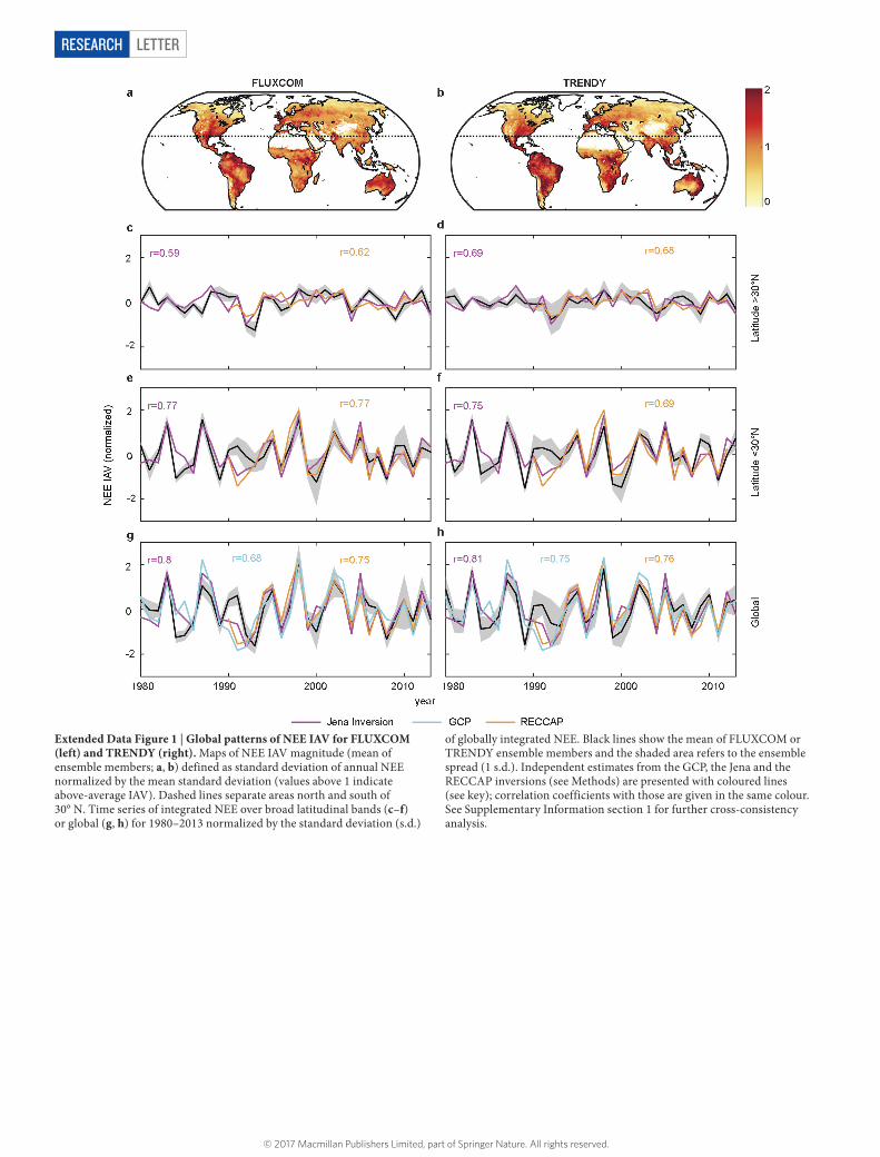
Extended Data Figure 1 | Global patterns of NEE IAV for FLUXCOM (left) and TRENDY (right). Maps of NEE IAV magnitude (mean of ensemble members; a, b) defined as standard deviation of annual NEE normalized by the mean standard deviation (values above 1 indicate above-average IAV). Dashed lines separate areas north and south of 30° N. Time series of integrated NEE over broad latitudinal bands (c–f) or global (g, h) for 1980–2013 normalized by the standard deviation (s.d.)

of globally integrated NEE. Black lines show the mean of FLUXCOM or TRENDY ensemble members and the shaded area refers to the ensemble spread (1 s.d.). Independent estimates from the GCP, the Jena and the RECCAP inversions (see Methods) are presented with coloured lines (see key); correlation coefficients with those are given in the same colour. See Supplementary Information section 1 for further cross-consistency analysis.

© 2017 Macmillan Publishers Limited, part of Springer Nature. All rights reserved.

LETTER RESEARCH

Extended Data Figure 2 | Local versus global dominance of NEETEMP versus NEEWAI for FLUXCOM and TRENDY ensemble members. Dots show individual ensemble members and the crosses show ensemble means with one standard deviation. Plotted is the difference of local NEEWAI and NEETEMP dominance (the difference of the leftmost blue and green data points in Fig. 2e and f) against the difference of global NEEWAI and NEETEMP dominance (the difference of the rightmost blue and green data points in Fig. 2e and f). The majority of ensemble members as well as ensemble means fall in the lower right quadrant, meaning an overall agreement that NEEWAI dominates at individual grid cells (local) but NEETEMP dominates the globally integrated flux anomaly (global).

© 2017 Macmillan Publishers Limited, part of Springer Nature. All rights reserved.

LETTERRESEARCH

Extended Data Figure 3 | Spatial patterns of covariance and correlation of WAI- and TEMP-driven GPP and TER IAV for TRENDY models. Maps of the covariance of annual anomalies (see equation (8) in Methods) of GPP and TER climatic components show large compensation effects (positive covariance) for WAI (a) but nearly no covariance for TEMP (c). Correlations between GPPWAI and TERWAI are large and everywhere

positive (b) while correlations among GPPTEMP and TERTEMP are weaker with a distinct spatial pattern of negative correlations in hot regions (d). All results refer to the mean of all TRENDY ensemble members. See Fig. 4 for equivalent FLUXCOM results, and Extended Data Fig. 4 for uncertainties.

© 2017 Macmillan Publishers Limited, part of Springer Nature. All rights reserved.

LETTER RESEARCH

Extended Data Figure 4 | Ensemble spread of covariation between TEMP and WAI components of GPP and TER for FLUXCOM and TRENDY. Plots show mean covariance (left) and correlation (right) between GPPTEMP and TERTEMP and GPPWAI and TERWAI for latitudinal bins of 5° for individual ensemble members (thin dotted lines) and ensemble mean (thick solid line with shaded area for 1 s.d.). Despite

uncertain magnitudes of GPPTEMP and TERTEMP correlation (large green-shaded area in right panels, b and d) their covariance is negligible (small green-shaded area in left panels, a and c). In comparison, there is large positive covariance of GPPWAI and TERWAI but its magnitude differs substantially among ensemble members (large blue-shaded area in left panels, a and c).

© 2017 Macmillan Publishers Limited, part of Springer Nature. All rights reserved.