Comparative Statics, Informativeness, and the - Northwestern
40
COMPARATIVE STATICS, INFORMATIVENESS, AND THE INTERVAL DOMINANCE ORDER By John K.-H. Quah and Bruno Strulovici Abstract: We identify a natural way of ordering functions, which we call the interval dominance order and develop a theory of monotone comparative statics based on this order. This way of ordering functions is weaker than the standard one based on the single crossing property (Milgrom and Shannon, 1994) and so our results apply in some settings where the single crossing property does not hold. For example, they are useful when examining the comparative statics of optimal stopping time prob- lems. We also show that certain basic results in statistical decision theory which are important in economics - specifically, the complete class theorem of Karlin and Rubin (1956) and the results connected with Lehmann’s (1988) concept of informativeness - generalize to payoff functions obeying the interval dominance order. Keywords: single crossing property, interval dominance order, supermodularity, comparative statics, optimal stopping time, complete class theorem, statistical de- cision theory, informativeness. JEL Classification Numbers: C61, D11, D21, F11, G11. Authors’ Emails: [email protected] [email protected] Acknowledgments: We would like to thank Ian Jewitt for many stimulating con- versations. 1
Transcript of Comparative Statics, Informativeness, and the - Northwestern

COMPARATIVE STATICS, INFORMATIVENESS, AND
THE INTERVAL DOMINANCE ORDER
By John K.-H. Quah and Bruno Strulovici
Abstract: We identify a natural way of ordering functions, which we call the interval
dominance order and develop a theory of monotone comparative statics based on this
order. This way of ordering functions is weaker than the standard one based on the
single crossing property (Milgrom and Shannon, 1994) and so our results apply in
some settings where the single crossing property does not hold. For example, they
are useful when examining the comparative statics of optimal stopping time prob-
lems. We also show that certain basic results in statistical decision theory which are
important in economics - specifically, the complete class theorem of Karlin and Rubin
(1956) and the results connected with Lehmann’s (1988) concept of informativeness
- generalize to payoff functions obeying the interval dominance order.
Keywords: single crossing property, interval dominance order, supermodularity,
comparative statics, optimal stopping time, complete class theorem, statistical de-
cision theory, informativeness.
JEL Classification Numbers: C61, D11, D21, F11, G11.
Authors’ Emails: [email protected] [email protected]
Acknowledgments: We would like to thank Ian Jewitt for many stimulating con-
versations.
1

1. Introduction
A central concept in the theory of monotone comparative statics is the single crossing
property.1 Let X be a subset of the real line R, and {f(·, s)}s∈S a family of functions
mapping X to R and parameterized by s in S ⊆ R. We say that this family is ordered
by the single crossing property if for all s′′ > s′ and x′′ > x′, the following holds:
f(x′′, s′)− f(x′, s′) ≥ (>) 0 =⇒ f(x′′, s′′)− f(x′, s′′) ≥ (>) 0. (1)
To keep our discussion simple, assume that f(·, s) has a unique maximum in X for
all s. The fundamental importance of the single crossing property (SCP) arises from
this result (Milgrom and Shannon (1994)): if the family {f(·, s)}s∈S is ordered by the
single crossing property, then argmaxx∈Xf(x, s) is increasing in s.
It is trivial to see that SCP is also necessary for comparative statics in the following
sense: if we require argmaxx∈Y f(x, s′′) ≥ argmaxx∈Y f(x, s′) for all Y ⊂ X whenever
s′′ > s′, then (1) must hold. (This is true since we could let Y be any set consisting
of two points in X.) In other words, SCP is necessary if we require the monotone
comparative statics conclusion to be robust to certain changes in the domain of the
objective functions.
However, SCP is not necessary for monotone comparative statics if we only require
argmaxx∈Y f(x, s′′) ≥ argmaxx∈Y f(x, s′) for Y = X or for Y belonging to a particular
subcollection of the subsets of X. To see this, consider Figures 1 and 2. In both cases,
we have argmaxx∈Xf(x, s′′) ≥ argmaxx∈Xf(x, s′); furthermore, argmaxx∈Y f(x, s′′) ≥
argmaxx∈Y f(x, s′) where Y is any closed interval contained in X. In Figure 1, SCP
is satisfied (specifically, (1) is satisfied) but this is not true in Figure 2. Consider
the points x′′ and x′ as depicted in Figure 2. We see that f(x′, s′) = f(x′′, s′) but
f(x′′, s′′) < f(x′, s′′), violating SCP.
1Early contributions to the literature on monotone comparative statics include Topkis (1978),
Milgrom and Roberts (1990), Vives (1990), and Milgrom and Shannon (1994). For a textbook
treatment see Topkis (1998).
2

The first objective of this paper is to develop a new way of ordering functions
that guarantees monotone comparative statics, whether the situation is like the one
depicted in Figure 1 or the one depicted in Figure 2. We call this new order the
interval dominance order. This order is more general than the one based on the
single crossing property. We show that it holds in some significant situations where
SCP does not hold; at the same time it retains many of the nice comparative statics
properties associated with SCP.
The second objective of this paper is to bridge the gap between the literature on
monotone comparative statics and the closely related literature in statistical decision
theory on informativeness. We refer in particular to Lehmann’s concept of informa-
tiveness (1988) which in turn builds on the complete class theorem of Karlin and
Rubin (1956).2 In that setting, the state of the world is unknown and the agent has
to take an action based on an observed signal, which conveys information on the true
state. Karlin and Rubin identify conditions under which optimal decision rules (in
some well-defined sense) must be monotone, i.e., the agent’s action is higher when
he receives a higher signal.3 Lehmann shows how we may compare the informative-
ness of two families of signals (or experiments) when the optimal decision rules are
monotone.
A crucial assumption in the Karlin-Rubin and Lehmann theorems is that the
agent’s payoff in state s when she takes action x, which we write as f(x, s), has
the following property: f(·, s) is a quasiconcave function of x, achieving a maximum
at x(s), with x increasing in s (like the situation depicted in Figure 2). However,
their results do not cover the case where {f(·, s)}s∈S is ordered by the single crossing
property. Amongst other things, SCP allows for non-quasiconcave payoff functions
(see Figure 2); indeed this feature is crucial to many of its economics applications.
2Economic applications of Lehmann’s concept of informativeness can be found in Persico (2000),
Athey and Levin (2001), Levin (2001), Bergemann and Valimaki (2002), and Jewitt (2006).3In other words, monotone decision rules form a complete class.
3

In short, the standard results on comparative informativeness accommodates the
situation depicted in Figure 2 but not that in Figure 1, whereas the standard results
on comparative statics accommodate the situation in Figure 1 but not that in Figure
2.
We generalize the Karlin-Rubin and Lehmann results by showing that their conclu-
sions hold even when the payoff functions {f(·, s)}s∈S satisfy the interval dominance
order. In this way, we obtain a single condition on the payoff functions that is use-
ful for both comparative statics and comparative informativeness, so results in one
category extend seamlessly into results in the other.
The rest of this paper is organized as follows. In Section 2, we define the interval
dominance order, explore its properties, and develop a comparative statics theorem.
Section 3 is devoted to applications. In Section 4 we show that the concept of IDO can
be easily extended to settings with uncertainty and that it is useful in that context.
Lehmann’s concept of informativeness is introduced in Section 5 and we demonstrate
its relevance for payoff functions obeying the interval dominance order. Finally, we
generalize Karlin and Rubin’s complete class theorem in Section 6.
2. The Interval Dominance Order
We begin by showing how a situation like that depicted in Figure 2, involving a
violation of SCP, can arise naturally in an economic setting.
Example 1. Consider a firm producing some good whose price we assume is fixed
at 1 (either because of market conditions or for some regulatory reason). It has
to decide on the production capacity (x) of its plant. Assume that a plant with
production capacity x costs Dx, where D is a positive scalar. Let s be the state of
the world, which we also identify with the demand for the good. The marginal cost
of producing the good in state s is c(s). We assume that, for all s, D + c(s) < 1.
The firm makes its capacity decision before the state of the world is realized and its
4

production decision after the state is revealed.
Suppose it chooses capacity x and the realized state of the world (and thus realized
demand) is s ≥ x. In this case, the firm should produce up to its capacity, so that its
profit Π(x, s) = x − c(s)x −Dx. On the other hand, if s < x, the firm will produce
(and sell) s units of the good, giving it a profit of Π(x, s) = s− c(s)s−Dx. It is easy
to see that Π(·, s) is increasing linearly for x ≤ s and thereafter declines, linearly with
a slope of −D. Its maximum is achieved at x = s, with Π(s, s) = (1 − c(s) − D)s.
Suppose s′′ > s′ and c(s′′) > c(s′). In other words, the state with higher demand also
has higher marginal cost. Then it is clear that the situation depicted in Figure 2 can
arise, with f(·, s′) = Π(·, s′) and f(·, s′′) = Π(·, s′′).
Let X be a subset of R and f and g two real-valued functions defined on X. We
say that g dominates f by the single crossing property (which we denote by g �SC f)
if for all x′′ and x′ such that x′′ > x′, the following holds:
f(x′′)− f(x′) ≥ (>) 0 =⇒ g(x′′)− g(x′) ≥ (>) 0. (2)
A family of real-valued functions {f(·, s)}s∈S, defined on X and parameterized by s
in S ⊂ R is referred to as an SCP family if the functions are ordered by SCP, i.e.,
whenever s′′ > s′, we have f(·, s′′) �SC f(·, s′).
In Figure 2, we have argmaxx∈R+f(x, s′′) > argmaxx∈R+
f(x, s′) even though
f(·, s′′) does not dominate f(·, s′) by SCP. Notice, however, that violations of (2)
can only occur if we compare points x′ and x′′ on opposite sides of the maximum
point of f(·, s′). This suggests that a possible way of weakening SCP, while retaining
comparative statics, is to require (2) to hold only for a certain collection of pairs
{x′, x′′}, rather than all possible pairs.
The set J is an interval of X if, whenever x′ and x′′ are in J , any element x in X
such that x′ ≤ x ≤ x′′ is also in J .4 Let f and g be two real-valued functions defined
4Note that X need not be an interval in the conventional sense, i.e., X need not be, using our
5
on X. We say that g dominates f by the interval dominance order (or, for short, g
I-dominates f , with the notation g �I f) if (2) holds for x′′ and x′ such that x′′ > x′
and f(x′′) ≥ f(x) for all x in the interval [x′, x′′] = {x ∈ X : x′ ≤ x ≤ x′′}.
Clearly, the interval dominance order (IDO) is weaker than ordering by SCP. For
example, in Figure 2, f(·, s′′) I-dominates f(·, s′) but f(·, s′′) does not dominate f(·, s′)
by SCP.
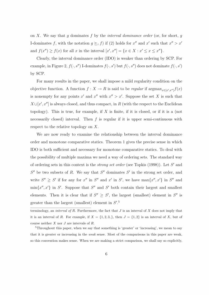
For many results in the paper, we shall impose a mild regularity condition on the
objective function. A function f : X → R is said to be regular if argmaxx∈[x′,x′′]f(x)
is nonempty for any points x′ and x′′ with x′′ > x′. Suppose the set X is such that
X∪[x′, x′′] is always closed, and thus compact, in R (with the respect to the Euclidean
topology). This is true, for example, if X is finite, if it is closed, or if it is a (not
necessarily closed) interval. Then f is regular if it is upper semi-continuous with
respect to the relative topology on X.
We are now ready to examine the relationship between the interval dominance
order and monotone comparative statics. Theorem 1 gives the precise sense in which
IDO is both sufficient and necessary for monotone comparative statics. To deal with
the possibility of multiple maxima we need a way of ordering sets. The standard way
of ordering sets in this context is the strong set order (see Topkis (1998)). Let S ′ and
S ′′ be two subsets of R. We say that S ′′ dominates S ′ in the strong set order, and
write S ′′ ≥ S ′ if for any for x′′ in S ′′ and x′ in S ′, we have max{x′′, x′} in S ′′ and
min{x′′, x′} in S ′. Suppose that S ′′ and S ′ both contain their largest and smallest
elements. Then it is clear that if S ′′ ≥ S ′, the largest (smallest) element in S ′′ is
greater than the largest (smallest) element in S ′.5
terminology, an interval of R. Furthermore, the fact that J is an interval of X does not imply that
it is an interval of R. For example, if X = {1, 2, 3, }, then J = {1, 2} is an interval of X, but of
course neither X nor J are intervals of R.5Throughout this paper, when we say that something is ‘greater’ or ‘increasing’, we mean to say
that it is greater or increasing in the weak sense. Most of the comparisons in this paper are weak,
so this convention makes sense. When we are making a strict comparison, we shall say so explicitly,
6

Theorem 1: Suppose that f and g are real-valued functions defined on X ⊂ R
and g �I f . Then the following property holds:
(?) argmaxx∈Jg(x) ≥ argmaxx∈Jf(x) for any interval J of X.
Furthermore, if property (?) holds and g is regular, then g �I f .
Proof: Assume that g I-dominates f and that x′′ is in argmaxx∈Jf(x) and x′ is
in argmaxx∈Jg(x). We need only consider the case where x′′ > x′. Since x′′ is in
argmaxx∈Jf(x), we have f(x′′) ≥ f(x) for all x in [x′, x′′] ⊆ J . Since g �I f , we also
have g(x′′) ≥ g(x′); thus x′′ is in argmaxx∈Jg(x). Furthermore, f(x′′) = f(x′) so that
x′ is in argmaxx∈Jf(x). If not, f(x′′) > f(x′) which implies (by the fact that g �I f)
that g(x′′) > g(x′), contradicting the assumption that g is maximized at x′.
To prove the other direction, we assume that there is an interval [x′, x′′] such that
f(x′′) ≥ f(x) for all x in [x′, x′′]. This means that x′′ is in argmaxx∈[x′,x′′]f(x). There
are two possible violations of IDO. One possibility is that g(x′) > g(x′′); in this case,
by the regularity of g, the set argmaxx∈[x′,x′′]g(x) is nonempty but does not contain
x′′, which violates (?). Another possible violation of IDO occurs if g(x′′) = g(x′)
but f(x′′) > f(x′). In this case, the set argmaxx∈[x′,x′′]g(x) either contains x′, which
violates (?) since argmaxx∈[x′,x′′]f(x) does not contain x′, or it contains some element
distinct from x′′, which also violates (?). QED
For the interval dominance order to be useful in applications, we need some simple
ways of checking that the property holds. For this purpose, the next result is crucial.
Proposition 1: Suppose that X is an interval of R and the functions f , g :
X → R are absolutely continuous on compact intervals in X (and thus f and g are
differentiable a.e.). If there is an increasing and positive function α : X → R such
that g′(x) ≥ α(x)f ′(x) a.e., then g �I f .
If the function α in Proposition 1 is a constant α, then we obtain g(x′′)− g(x′) ≥
α(f(x′′) − f(x′)), which implies g �SC f . When α is not a constant, the functions f
and g in Proposition 2 need not be related by SCP, as the following example shows.
as in ‘strictly higher’, ‘strictly increasing’, etc.
7

Let f : [0,M ] → R be a differentiable and quasiconcave function, with f(0) = 0
and a unique maximum at x∗ in (0,M). Let α : [0,M ] → R be given by α(x) = 1
for x ≤ x∗ and α(x) = 1 + (x − x∗) for x > x∗. Consider g : [0,M ] satisfying
g(0) = f(0) = 0 with g′(x) = α(x)f ′(x) (as in Proposition 1). Then it is clear
that g(x) = f(x) for x ≤ x∗ and g(x) < f(x) for x > x∗. The function g is also
quasiconcave with a unique maximum at x∗ and g I-dominates f , but g does not
dominate f by SCP.
Proposition 1 is a consequence of the following lemma.
Lemma 1: Suppose [x′, x′′] is a compact interval of R and α and h are real-valued
functions defined on [x′, x′′], with h integrable and α increasing (and thus integrable
as well). If∫ x′′
xh(t)dt ≥ 0 for all x in [x′, x′′], then∫ x′′
x′α(t)h(t)dt ≥ α(x′)
∫ x′′
x′h(t)dt. (3)
Proof: We confine ourselves to the case where α is an increasing and differentiable
function. If we can establish (3) for such functions, then we can extend it to all
increasing functions α since any such function can be approximated by an increasing
and differentiable function.
The function H(t) = α(t)∫ x′′
th(z)dz is absolutely continuous and thus differ-
entiable a.e.; by the fundamental theorem of calculus, we have H(x′′) − H(x′) =∫ x′
x′′ H′(t)dt. Note that H(x′′) = 0 and that by the product rule,
H ′(t) = α′(x)
∫ x′′
t
h(z)dz − α(t)h(t).
So
−H(x′) = −α(x′)
∫ x′′
x′h(t)dt =
∫ x′′
x′α′(x)
(∫ x′′
t
h(z)dz
)dt−
∫ x′′
x′α(t)h(t)dt.
Note that the first term on the right of this equation is always nonnegative by as-
sumption and so we obtain (3). QED
8

Proof of Proposition 1: Consider x′′ and x′ in X such that x′′ > x′ and assume
that f(x) ≤ f(x′′) for all x in [x′, x′′]. Since f is absolutely continuous on [x′, x′′],
f(x′′)− f(x) =∫ x∗
xf ′(t)dt (with an analogous expression for g). We then have∫ x′′
x
g′(t)dt ≥∫ x′′
x
α(t)f ′(t)dt ≥ α(x′)
∫ x′′
x′f ′(t)dt,
where the second inequality follows from Lemma 1. So
g(x′′)− g(x′) = α(x′)(f(x′′)− f(x′)) (4)
and g(x′′) ≥ (>)g(x′) if f(x′′) ≥ (>)f(x′). QED
Another familiar concept in the theory of monotone comparative statics, and one
which is stronger than SCP, is the concept of increasing differences (see Milgrom
and Shannon (1994) and Topkis (1998)). The function g dominates f by increasing
differences (see Milgrom and Shannon (1994) and Topkis (1998)) if for any x′′ and x′
in X, with x′′ > x′, we have
g(x′′)− g(x′) ≥ f(x′′)− f(x′). (5)
We say that a function g dominates f by conditional increasing differences (and
denote it by g �IN f) if (5) holds for all pairs x′ and x′′ in X such that f(x′′) ≥ f(x)
for x in [x′, x′′]. Clearly, if g dominates f by conditional increasing differences then
g I-dominates f . The next result gives sufficient conditions under which g and f can
be related in this manner.
Proposition 2: Suppose X is an interval of R and the functions f , g : X → R
are absolutely continuous on compact intervals in X (and thus f and g are differen-
tiable a.e.). If there is an increasing function α : X → R with α(x) ≥ 1 for all x in
X such that g′(x) ≥ α(x)f ′(x) a.e., then g �IN f .
Proof: Retrace the proof of Proposition 1; the result follows from (4). QED
9
Many problems in economic theory involves the maximization of the difference
between benefits and costs arising from some activity. The next result shows the
relevance of conditional increasing differences to problems of this sort.
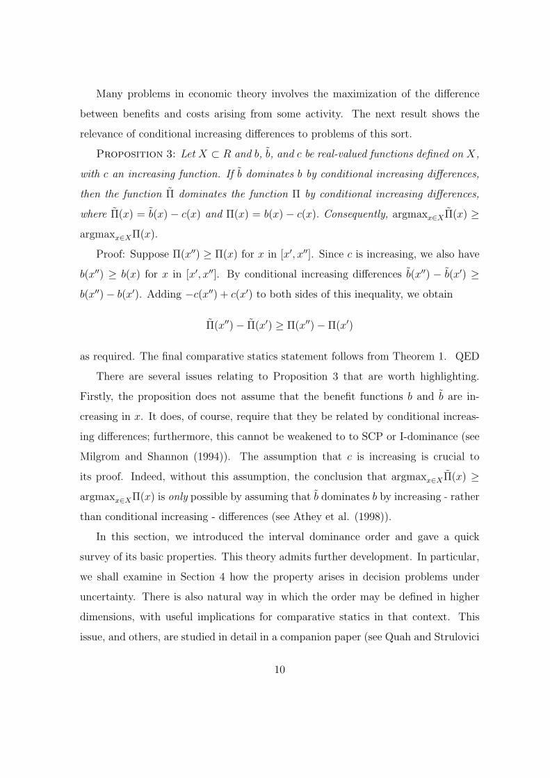
Proposition 3: Let X ⊂ R and b, b, and c be real-valued functions defined on X,
with c an increasing function. If b dominates b by conditional increasing differences,
then the function Π dominates the function Π by conditional increasing differences,
where Π(x) = b(x) − c(x) and Π(x) = b(x) − c(x). Consequently, argmaxx∈XΠ(x) ≥
argmaxx∈XΠ(x).
Proof: Suppose Π(x′′) ≥ Π(x) for x in [x′, x′′]. Since c is increasing, we also have
b(x′′) ≥ b(x) for x in [x′, x′′]. By conditional increasing differences b(x′′) − b(x′) ≥
b(x′′)− b(x′). Adding −c(x′′) + c(x′) to both sides of this inequality, we obtain
Π(x′′)− Π(x′) ≥ Π(x′′)− Π(x′)
as required. The final comparative statics statement follows from Theorem 1. QED
There are several issues relating to Proposition 3 that are worth highlighting.
Firstly, the proposition does not assume that the benefit functions b and b are in-
creasing in x. It does, of course, require that they be related by conditional increas-
ing differences; furthermore, this cannot be weakened to to SCP or I-dominance (see
Milgrom and Shannon (1994)). The assumption that c is increasing is crucial to
its proof. Indeed, without this assumption, the conclusion that argmaxx∈XΠ(x) ≥
argmaxx∈XΠ(x) is only possible by assuming that b dominates b by increasing - rather
than conditional increasing - differences (see Athey et al. (1998)).
In this section, we introduced the interval dominance order and gave a quick
survey of its basic properties. This theory admits further development. In particular,
we shall examine in Section 4 how the property arises in decision problems under
uncertainty. There is also natural way in which the order may be defined in higher
dimensions, with useful implications for comparative statics in that context. This
issue, and others, are studied in detail in a companion paper (see Quah and Strulovici
10
(2007)). The next section is devoted to applying the theoretical results obtained so
far; readers interested in a quick overview of the theory can skip the next section.
3. Applications of the IDO property
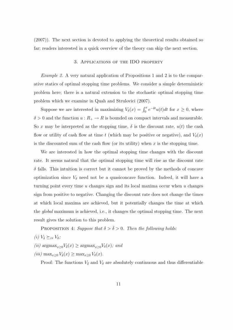
Example 2. A very natural application of Propositions 1 and 2 is to the compar-
ative statics of optimal stopping time problems. We consider a simple deterministic
problem here; there is a natural extension to the stochastic optimal stopping time
problem which we examine in Quah and Strulovici (2007).
Suppose we are interested in maximizing Vδ(x) =∫ x
0e−δtu(t)dt for x ≥ 0, where
δ > 0 and the function u : R+ → R is bounded on compact intervals and measurable.
So x may be interpreted as the stopping time, δ is the discount rate, u(t) the cash
flow or utility of cash flow at time t (which may be positive or negative), and Vδ(x)
is the discounted sum of the cash flow (or its utility) when x is the stopping time.
We are interested in how the optimal stopping time changes with the discount
rate. It seems natural that the optimal stopping time will rise as the discount rate
δ falls. This intuition is correct but it cannot be proved by the methods of concave
optimization since Vδ need not be a quasiconcave function. Indeed, it will have a
turning point every time u changes sign and its local maxima occur when u changes
sign from positive to negative. Changing the discount rate does not change the times
at which local maxima are achieved, but it potentially changes the time at which
the global maximum is achieved, i.e., it changes the optimal stopping time. The next
result gives the solution to this problem.
Proposition 4: Suppose that δ > δ > 0. Then the following holds:
(i) Vδ �IN Vδ;
(ii) argmaxx≥0Vδ(x) ≥ argmaxx≥0Vδ(x); and
(iii) maxx≥0 Vδ(x) ≥ maxx≥0 Vδ(x).
Proof: The functions Vδ and Vδ are absolutely continuous and thus differentiable
11

a.e.; moreover,
V ′δ (x) = e−δxu(x) = e(δ−δ)xV ′
δ (x).
Note that the function α(x) = e(δ−δ)x is increasing and greater than 1. So part (i)
follows from Proposition 2 and part (ii) from Theorem 1. For (iii), let us suppose
that Vδ(x) is maximized at x = x∗. Then for all x in [0, x∗], Vδ(x) ≤ Vδ(x∗). Since
Vδ(0) = Vδ(0) = 0, the fact that Vδ �IN Vδ now guarantees that Vδ(x∗) ≥ Vδ(x
∗).
Finally, note that maxx≥0 Vδ(x) ≥ Vδ(x∗). QED
Example 3. Consider a firm that chooses output x to maximize profit, given by
Π(x) = xP (x) − C(x), where P is the inverse demand function and C is the cost
function. Imagine that there is a change in market conditions, so that the both P
and C are changed to P and C respectively. When can we say that argmaxx≥0Π(x) ≥
argmaxx≥0Π(x)? By Theorem 1, this holds if Π I-dominates Π. Intuitively, we will
expect this to hold if the increase in the inverse demand is greater than any increase
in costs. This idea can be formalized in the following manner.
Assume that all the functions are differentiable, that P and P take strictly positive
values, and that the cost functions are strictly increasing. Define a(x) = Π(x)/Π(x).
Then
Π′(x) = a′(x)xP (x) + a(x)(xP (x))′ − C ′(x)
≥ a(x)(xP (x))′ −
[C ′(x)
C ′(x)
]C ′(x),
where the inequality follows since xP (x) > 0. Now suppose we make we assume that
a(x) =P (x)
P (x)≥ C ′(x)
C ′(x), (6)
then we obtain Π′(x) ≥ a(x)Π′(x). By Proposition 1, Π I-dominates Π if a is increasing
and (6) holds; in other words, the ratio of the inverse demand functions is increasing
in x and greater than the ratio of the marginal costs.6
6Note that our argument does not require that P be decreasing in x.
12

Example 4. The perceptive reader will notice that Proposition 1 and Lemma 1
when presented in a somewhat different context are in fact very familiar since they
are closely related to standard results on stochastic dominance. For example, recall
that a density function γ defined on some interval [a, b] in R is said to first order
stochastically dominate another density function β defined on the same interval if∫ x
aβ(t)dt ≥
∫ x
aγ(t)dt for all x in [a, b]. It is well known that this implies that for any
increasing and bounded utility function u defined on [a, b], we have∫ b
a
u(t)γ(t)dt ≥∫ b
a
u(t)β(t)dt ; (7)
in other words, the expected utility of γ is greater than that of β.
One could think of this basic result as an application of the theory developed
here. If γ first order stochastically dominates β then f : [a, b] → R defined by f(x) =∫ x
a(γ(t)− β(t)) dt has the following properties: f(a) = f(b) = 0 and f(x) ≤ 0 = f(b)
for all x in [a, b]. By Proposition 1, the function g defined by
g(x) =
∫ x
a
u(t) (γ(t)− β(t)) dt
I-dominates f since g′(x) = u(x)f ′(x). So g(b) ≥ g(a) = 0, which gives us (7).
4. The interval dominance order when the state is uncertain
Consider the following problem. Let {f(·, s)}s∈S be a family of functions parame-
terized by s in S, an interval of R, with each function f(·, s) mapping Y , an interval of
R, to R. Assume that all the functions are quasiconcave, with their peaks increasing
in s; by this we mean that argmaxx∈Y f(x, s′′) ≥ argmaxx∈Y f(x, s′) whenever s′′ > s′.
(Note that since each function f(·, s) is quasiconcave, it either has a unique maximizer
or they must form an interval.) We shall refer to such a family of functions as a QCIP
family, where QCIP stands for quasiconcave with increasing peaks. Interpreting s to
be the state of the world, an agent has to choose x under uncertainty, i.e., before
13

s is realized. We assume the agent maximizes the expected value of his objective;
formally, he maximizes
F (x, λ) =
∫s∈S
f(x, s)λ(s)ds,
where λ : S → R is the density function defined over the states of the world. It
is natural to think that if the agent considers the higher states to be more likely,
then his optimal value of x will increase. Is this true? More generally, we can ask
the same question if the functions {f(·, s)}s∈S form an IDO family, i.e., a family of
regular functions f(·, s) : X → R, with X ⊆ R, such that f(·, s′′) I-dominates f(·, s′)
whenever s′′ > s′.
One way of formalizing the notion that higher states are more likely is via the
monotone likelihood ratio (MLR) property. Let λ and γ be two density functions
defined on the interval S of R and assume that λ(s) > 0 for s in S. We call γ an
MLR shift of λ if γ(s)/λ(s) is increasing in s. For density changes of this kind, there
are two results that come close, though not quite, to addressing the problem we posed.
Ormiston and Schlee (1993) identify some conditions under which an upward
MLR shift in the density function will raise the agent’s optimal choice. Amongst
other conditions, they assume that F (·;λ) is quasiconcave. This will hold if all the
functions in the family {f(·, s)}s∈S are concave but will not generally hold if the
functions are just quasiconcave. Athey (2002) has a related result which says that an
upward MLR shift will lead to a higher optimal choice of x provided {f(·, s)}s∈S is
an SCP family. As we had already pointed out in Example 1, a QCIP family need
not be an SCP family.
The next result gives the solution to the problem we posed.
Theorem 2: Let S be an interval of R and {f(·, s)}s∈S be an IDO family. Then
F (·, γ) �I F (·, λ) if γ is an MLR shift of λ. Consequently, argmaxx∈XF (x, γ) ≥
argmaxx∈XF (x, λ).
Notice that since {f(·, s)}s∈S in Theorem 2 is assumed to be an IDO family, we
know (from Theorem 1) that argmaxx∈Xf(x, s′′) ≥ argmaxx∈Xf(x, s′). Thus Theorem
14

2 guarantees that the comparative statics which holds when s is known also holds
when s is unknown but experiences an MLR shift.7
The proof of Theorem 2 requires a lemma (stated below). Its motivation arises
from the observation that if g �SC f , then for any x′′ > x′ such that g(x′)− g(x′′) ≥
(>) 0, we must also have f(x′)− f(x′′) ≥ (>) 0. Lemma 2 is the (less trivial) analog
of this observation in the case when g �I f .
Lemma 2: Let X be a subset of R and f and g two regular functions defined on
X. Then g �I f if and only if the following property holds:
(M) if g(x′) ≥ g(x) for x in [x′, x′′] then
g(x′)− g(x′′) ≥ (>) 0 =⇒ f(x′)− f(x′′) ≥ (>) 0.
Proof: Suppose x′ < x′′ and g(x′) ≥ g(x) for x in [x′, x′′]. There are two possible
ways for property (M) to be violated. One possibility is that f(x′′) > f(x′). By
regularity, we know that argmaxx∈[x′,x′′]f(x) is nonempty; choosing x∗ in this set, we
have f(x∗) ≥ f(x) for all x in [x′, x∗], with f(x∗) ≥ f(x′′) > f(x′). Since g �I f , we
must have g(x∗) > g(x′), which is a contradiction.
The other possible violation of (M) occurs if g(x′) > g(x′′) but f(x′) = f(x′′). By
regularity, we know that argmaxx∈[x′,x′′]f(x) is nonempty, and if f is maximized at x∗
with f(x∗) > f(x′), then we are back to the case considered above. So assume that
x′ and x′′ are both in argmaxx∈[x′,x′′]f(x). Since f �I g, we must have g(x′′) ≥ g(x′),
contradicting our initial assumption.
So we have shown that (M) holds if g �I f . The proof that (M) implies g �I f is
similar. QED
Proof of Theorem 2: This consists of two parts. Firstly, we prove that if F (x′′, λ) ≥
F (x, λ) for all x in [x′, x′′], then, for any s in S,∫ s∗
s
(f(x′′, s)− f(x′, s))λ(s)ds ≥ 0 (8)
7We are echoing an observation that was also made by Athey (2002) in a similar context.
15
(where s∗ denotes the supremum of S). Assume instead that there is s such that∫ s∗
s
(f(x′′, s)− f(x′, s))λ(s)ds < 0. (9)
By the regularity of f(·, s), there is x that maximizes f in [x′, x′′]. In particular,
f(x, s) ≥ f(x, s) for all x in [x, x′′]. Since {f(·, s)}s∈S is an IDO family of regular
functions, we also have f(x, s) ≥ f(x′′, s) for all s ≤ s (using Lemma 2). Thus∫ s
s∗
(f(x, s)− f(x′′, s))λ(s)ds ≥ 0, (10)
where s∗ is the infimum of S. Notice also that f(x, s) ≥ f(x, s) for all x in [x′, x],
which implies that f(x, s) ≥ f(x′, s) for all s ≥ s. Aggregating across s we obtain∫ s∗
s
(f(x, s)− f(x′, s))λ(s)ds ≥ 0. (11)
It follows from (9) and (11) that∫ s∗
s
(f(x, s)− f(x′′, s))λ(s)ds =
∫ s∗
s
(f(x, s)− f(x′, s))λ(s)ds
+
∫ s∗
s
(f(x′, s)− f(x′′, s))λ(s)ds
> 0.
Combining this with (10), we obtain∫ s∗
s∗
(f(x, s)− f(x′′, s))λ(s)ds > 0 ;
in other words, F (x, λ) > F (x′′, λ) which is a contradiction.
Given (8), the function H(·, λ) : [s∗, s∗] → R defined by
H(s, λ) =
∫ s
s∗
(f(x′′, s)− f(x′, s)) γ(s)ds
satisfies H(s∗, λ) ≥ H(s, λ) for all s in [s∗, s∗]. Defining H(·, γ) in an analogous fash-
ion, we also have H ′(s, γ) = [γ(s)/λ(s)]H ′(s, λ) for s in S. Since γ is an upward MLR
shift of λ, the ratio γ(s)/λ(s) is increasing in s. By Proposition 1, H(·, γ) �I H(·, λ).
16

In particular, we have H(s∗, γ) ≥ (>)H(s∗, γ) = 0 if H(s∗, λ) ≥ (>)H(s∗, λ) = 0.
Re-writing this, we have F (x′′, γ) ≥ (>)F (x′, γ) if F (x′′, λ) ≥ (>)F (x′, λ). QED
Note that Theorem 2 remains true if S is not an interval; in Appendix A, we prove
Theorem 2 in the case where S is a finite set of states.
We turn now to two applications of Theorem 2.
Example 1 continued. Recall that in state s, the firm’s profit is Π(x, s). It achieves
its maximum at x∗(s) = s, with Π(s, s) = (1 − c(s) − D)s, which is strictly pos-
itive by assumption. The firm has to choose its capacity before the state of the
world is realized; we assume that s is drawn from S, an interval in R, and has
a distribution given by the density function λ : S → R. We can think of the
firm as maximizing its expected profit, which is∫
SΠ(x, s)λ(s)ds, or more generally,
let us assume that it maximizes the expected utility from profit, i.e., it maximizes
F (x, λ) =∫
Su(Π(x, s), s)λ(s)ds, where, for each s, the function u(·, s) : R → R is
strictly increasing. The family {u(Π(·, s), s)}s∈S consists of quasiconcave functions,
the peaks of which are increasing in s. By Theorem 2, we know that an upward MLR
shift of the density function will lead the firm to choose a greater capacity.
Example 5. Consider a firm that has to decide on when to launch a new product.
The more time the firm gives itself, the more it can improve the quality of the product
and its manufacturing process, but it also knows that there is a rival about to launch
a similar product. In formal terms, we assume that the firm’s profit (if it is not
anticipated by its rival) is an increasing function of time π : R+ → R+. If the
rival launches its product at time s, then the firm’s profit falls to w(s) (in R). In
other words, the firm’s profit in state s is π(t, s) = π(t) for t ≤ s and w(s) for
t > s, where w(s) < π(s). Clearly, each π(·, s) is a quasiconcave function and
{π(·, s)}s∈S is an IDO family. The firm decides on the launch date t by maximizing
F (t, λ) =∫
s∈Sπ(t, s)λ(s)ds, where λ : R+ → R is the density function over s. By
Theorem 2, if the firm thinks that it is less likely that the rival will launch early,
in the sense that there is an upward MLR shift in the density function, then it will
17
decide on a later launch date.
Note that we impose no restrictions on the function w : R+ → R, which gives
the firm’s profit should it be anticipated by its rival at time s. If w is an increasing
function of s, then one can check that {π(·, s)}s∈S is an SCP-ordered family, but
Theorem 2 gives us the desired conclusion without making this stronger assumption.
5. Comparing Information Structures8
Consider an agent who, as in the previous section, has to make a decision before
the state of the world (s) is realized, where the set of possible states S is a subset of
R. In this section we assume that the decision x is picked from a finite set X in R.
Suppose that, before he makes his decision, the agent observes a signal z. This signal
is potentially informative of the true state of the world; we refer to the collection
{H(·|s)}s∈S , where H(·|s) is the distribution of the signal z conditional on s, as the
information structure of the decision maker’s problem. (Whenever convenient, we
shall simply call this information structure H.) We assume that, for every s, H(·|s)
admits a density function and has the compact interval Z as its support. We say that
H is MLR-ordered if H(·|s′′) is an MLR shift of H(·|s′) whenever s′′ > s′.
We assume that the agent has a prior distribution λ on S. We allow either of the
following: (i) S is a compact interval and λ admits a density function with S as its
support or (ii) S is finite and λ has S as its support.
The agent’s decision rule (under H) is a map from Z to X. We denote his
posterior distribution (on S) upon observing z by λzH ; so the agent with a decision
rule φ : Z → X will have an ex ante utility given by
U(φ,H, λ) =
∫z∈Z
[∫s∈S
u(φ(z), s)dλzH
]dMH,λ =
∫Z×S
u(φ(z), s) dJH,λ
where MH,λ is the marginal distribution of z and JH,λ the joint distribution of (z, s)
given H and λ. A decision rule φ : Z → X that maximizes the agent’s (posterior)
8We are very grateful to Ian Jewitt for introducing us to the literature in this section and the
next and for extensive discussions.
18

expected utility at each realized signal is called anH-optimal decision rule. We denote
the agent’s ex ante utility using such a rule by V(H, λ, u).
Consider now an alternative information structure given by the collection {G(·|s)}s∈S;
we assume that G(·|s) admits a density function and has the compact interval Z as
its support. What conditions will guarantee that the information structure H is more
favorable than G in the sense of offering the agent a higher ex ante utility; in other
words, how can we guarantee that V(H, λ, u) ≥ V(G, λ, u)?
It is well known that this holds if H is more informative than G according to the
criterion developed by Blackwell (1953); furthermore, this criterion is also necessary if
one does not impose significant restrictions on u (see Blackwell (1953) or, for a recent
textbook treatment, Gollier (2001)). We wish instead to consider the case where a
significant restriction is imposed on u; specifically, we assume that {u(·, s)}s∈S is an
IDO family. We show that, in this context, a different notion of informativeness due
to Lehmann (1988) is the appropriate concept.9
Our assumptions on H guarantee that, for any s, H(·|s) admits a density function
with support Z; therefore, for any (z, s) in Z × S, there exists a unique element in
Z, which we denote by T (z, s), such that H(T (z, s)|s) = G(z|s). We say that H is
more accurate than G if T is an increasing function of s.10 Our goal in this section is
to prove the following result.
Theorem 3: Suppose {u(·, s)}s∈S is an IDO family, G is MLR-ordered, and λ is
the agent’s prior distribution on S. If H is more accurate than G, we obtain
V(H, λ, u) ≥ V(G, λ, u). (12)
9For a discussion of the advantages of Lehmann’s concept over Blackwell’s, see Lehmann (1988)
and Persico (2000). Some papers with economic applications of Lehmann’s concept of informative-
ness are Persico (2000), Athey and Levin (2001), Levin (2001), Bergemann and Valimaki (2002),
and Jewitt (2006). Athey and Levin’s paper also explores other related concepts of informativeness
and their relationship with the payoff functions.10The concept is Lehmann’s; the term accuracy follows Persico (2000).
19

This theorem generalizes a number of earlier results. Lehmann (1988) establishes
a special case of Theorem 3 in which {u(·, s)}s∈S is a QCIP family. Persico (1996)
has a version of Theorem 3 in which {u(·, s)}s∈S is an SCP family, but he requires the
optimal decision rule to vary smoothly with the signal, a property that is not generally
true without the sufficiency of the first order conditions for optimality. A proof of
Theorem 3 for the general SCP case can be found in Jewitt’s (2006) unpublished
notes.11
To prove Theorem 3, we first note that if G is MLR-ordered, then the family
of posterior distributions {λzH}z∈Z is also MLR-ordered, i.e., if z′′ > z′ then λz′′
H is
an MLR shift of λz′H .12 Since {u(·, s)}s∈S is an IDO family, Theorem 3 guarantees
that the G-optimal decision rule can be chosen to be increasing with z. Therefore,
Theorem 3 is valid if we can show that for any increasing decision rule ψ : Z → X
under G there is a rule φ : Z → X under H that gives a higher ex ante utility, i.e.,∫Z×S
u(φ(z), s)dJH,λ ≥∫
Z×S
u(ψ(z), s)dJG,λ.
This inequality in turn follows from aggregating (across s) the inequality (13) below.
Proposition 5: Suppose {u(·, s)}s∈S is an IDO family and H is more accurate
than G. Then for any increasing decision rule ψ : Z → X under G, there is an
increasing decision rule φ : Z → X under H such that, at each state s, the distribution
of utility induced by ψ and H(·|s) first order stochastically dominates the distribution
of utility induced by φ and G(·|s). Consequently, at each state s,∫z∈Z
u(φ(z), s)dH(z|s) ≥∫
z∈Z
u(ψ(z), s)dG(z|s). (13)
11However, there is at least one sense in which it is not correct to say that Theorem 3 generalizes
Lehmann’s result. The criterion employed by us here (and indeed by Persico (1996) and Jewitt
(2006) as well) - comparing information structures with the ex ante utility - is different from the
criterion Lehmann used. We return to this issue in the next section (specifically, Corollary 1), where
we compare information structures using precisely the same criterion as Lehmann’s.12This is not hard to prove; indeed, the two properties are equivalent.
20
(At a given state s, a decision rule ρ and a distribution on z induces a distribution
of utility in the following sense: for any measurable set U of R, the probability of
{u ∈ U} equals the probability of {z ∈ Z : u(ρ(z), s) ∈ U}. So it is meaningful to
refer, as this proposition does, to the distribution of utility at each s.)
Our proof of Proposition 5 requires the following lemma.
Lemma 3: Suppose {u(·, s)}s∈S is an IDO family and H is more accurate than
G. Then for any increasing decision rule ψ : Z → X under G, there is an increasing
decision rule φ : Z → X under H such that, for all (z, s),
u(φ(T (z, s)), s) ≥ u(ψ(z), s). (14)
Proof: We shall only demonstrate here the way in which we construct φ from
ψ; the fact that it is an increasing rule is proved in Appendix B. We shall confine
ourselves here to the case where S is a compact interval; the proof can be modified
in an obvious way to deal with the case where S is finite.
For every t in Z and s in S, there ia a unique z in Z such that t = T (z, s). This
follows from the fact that G(·|s) is a strictly increasing continuous function (since it
admits a density function with support Z). We write z = τ(t, s); note that because
T is increasing in both its arguments, the function τ : Z × S → Z is decreasing in s.
Note also that (14) is equivalent to
u(φ(t), s) ≥ u(ψ(τ(t, s)), s). (15)
We will now show φ(t) may be chosen to satisfy (15). We may partition S = [s∗, s∗∗]
into the sets S1, S2,..., SM , where M is odd, with the following properties: (i) if
m > n, then any element in Sm is greater than any element in Sn; (ii) whenever m is
odd, Sm is a singleton, with S1 = {s∗} and SM = {s∗∗}; (iii) when m is even, Sm is
an open interval; (iv) for any s′ and s′′ in Sm, we have ψ(τ(t, s′)) = ψ(τ(t, s′′)); and
(v) for s′′ in Sm and s′ in Sn such that m > n, ψ(τ(t, s′)) ≥ ψ(τ(t, s′′)).
21

In other words, we have partitioned S into finitely many sets, so that within each
set, the same action is taken under ψ and the actions are decreasing. This is possible
because X is finite, ψ is increasing in the signal and τ is decreasing in s. We denote
the action taken in Sm by ψm, with ψ1 ≥ ψ2 ≥ ψ3 ≥ ... ≥ ψM . Establishing (15)
involves finding φ(t) such that
u(φ(t), sm) ≥ u(ψm, sm) for any sm ∈ Sm; m = 1, 2, ...,M . (16)
In the interval [ψ2, ψ1], we pick the largest action φ2 that maximizes u(·, s∗) in
that interval. By the IDO property,
u(φ2, sm) ≥ u(ψm, sm) for any sm ∈ Sm; m = 1, 2. (17)
Recall that S3 is a singleton; we call that element s3. The action φ4 is chosen to be
the largest action in the interval [ψ4, φ2] that maximizes u(·, s3). Since ψ3 is in that
interval, we have u(φ4, s3) ≥ u(ψ3, s3). Since u(φ4, s3) ≥ u(ψ4, s3), the IDO property
guarantees that u(φ4, s4) ≥ u(ψ4, s4) for any s4 in S4. Using the IDO property again
(specifically, Lemma 2), we have u(φ4, sm) ≥ u(φ2, sm) for sm in Sm (m = 1, 2) since
u(φ4, s3) ≥ u(φ2, s3). Combining this with (17), we have found φ4 in [ψ4, φ2] such
that
u(φ4, sm) ≥ u(ψm, sm) for any sm ∈ Sm; m = 1, 2, 3, 4. (18)
We can repeat the procedure finitely many times, at each stage choosing φm+1 (for m
odd) as the largest element maximizing u(·, sm) in the interval [ψm+1, φm−1], and
finally, choosing φM+1 as the largest element maximizing u(·, s∗∗) in the interval
[ψM , φM−1]. It is clear that φ(t) = φM will satisfy (16). QED
Proof of Proposition 5: Let z denote the random signal received under information
structure G and let uG denote the (random) utility achieved when the decision rule ψ
is used. Correspondingly, we denote the random signal received under H by t, with
uH denoting the utility achieved by the rule φ, as constructed in Lemma 3. Observe
22
that for any fixed utility level u′ and at a given state s′,
Pr[uH ≤ u′|s = s′] = Pr[u(φ(t), s′) ≤ u′|s = s′]
= Pr[u(φ(T (z, s′)), s′) ≤ u′|s = s′]
≤ Pr[u(ψ(z), s′) ≤ u′|s = s′]
= Pr[uG ≤ u′|s = s′]
where the second equality comes from the fact that, conditional on s = s′, the dis-
tribution of t coincides with that of T (z, s′), and the inequality comes from the fact
that u(φ(T (z, s′)), s′) ≥ u(ψ(z), s′) for all z (by Lemma 3).
Finally, the fact that, given the state, the conditional distribution of uH first
order stochastically dominates uG means that the conditional mean of uH must also
be higher than that of uG. QED
As a simple application of Theorem 3, consider again Example 1, where a firm has
to decide on its production capacity before the state of the world is realized. Suppose
that before it makes its decision, the firm receives a signal z from the information
structure G. Provided G is MLR-ordered, we know that the posterior distributions
(on S) will also be MLR-ordered (in z). It follows from Theorem 2 that a higher
signal will cause the firm to decide on a higher capacity. Assuming the firm is risk
neutral, its ex ante expected profit is V(λ,G,Π), where λ is the firm’s prior on S.
Theorem 3 tells us that a more accurate information structure H will lead to a higher
ex ante expected profit; the difference V(λ, ,H,Π)−V(λ, ,G,Π) represents what the
firm is willing to spend for the more accurate information structure.
Our next example is a less straightforward application of Proposition 5.
Example 6. There are N investors, with investor i having wealth wi > 0 and the
strictly increasing Bernoulli utility function vi. These investors place their wealth
with a manager who has to decide on an investment policy; specifically, the manger
must allocate the total pool of funds W =∑N
i=1wi between a risky asset, with return
s in state s, and a safe asset with return r > 0. Denoting the fraction invested
23

in the risky asset by x, investor i’s utility (as a function of x and s) is given by
ui(x, s) = vi((xs + (1− x)r)wi). It is easy to see that {ui(·, s)}s∈S is an IDO family.
Indeed, we can say more: for s > r, ui(·, s) is strictly increasing in x; for s = r, ui(·, r)
is the constant vi(rwi); and for s < r, ui(·.s) is strictly decreasing in x.
Before she makes her portfolio decision, the manager receives a signal z from some
information structure G. She employs the decision rule ψ, where ψ(z) (in [0, 1]) is the
fraction of W invested in the risky asset. We assume that ψ is increasing in the signal.
(We shall justify this assumption in the next section.) Suppose that the manager
now has access to a superior information structure H. By Proposition 5, there is
an increasing decision rule φ under H such that, at any state s, the distribution of
investor k’s utility under H and φ first order stochastically dominates the distribution
of k’s utility under G and ψ. In particular, (13) holds for u = uk. Aggregating across
states we obtain Uk(φ,H, λk) ≥ Uk(ψ,G, λk), where λk is investor k’s (subjective)
prior; in other words, k’s ex ante utility is higher with the new information structure
and the new decision rule.
But even more can be said because, for any other investor i, ui(·, s) is a strictly
increasing transformation of uk(·, s), i.e., there is a strictly increasing function f such
that ui = f ◦uk. It follows from Proposition 5 that (13) is true, not just for u = uk but
for u = ui. Aggregating across states, we obtain Ui(φ,H, λi) ≥ Ui(ψ,G, λi), where λi
is investor i’s prior.
To summarize, we have shown the following: though different investors may have
different attitudes towards risk aversion and different priors, the greater accuracy of
H compared to G allows the manager to implement a new decision rule that gives
greater ex ante utility to every investor.
Finally, we turn to the following question: how important is the accuracy criterion
to the results in this section? For example, we may wonder if the conclusion in
Theorem 3 is, in a sense, too strong. Theorem 3 tells us that when H is more
24
accurate than G, it gives the agent a higher ex ante utility for any prior that he may
have on S. This raises the possibility that the accuracy criterion may be weakened if
we only wish H to give a higher ex ante utility than G for a particular prior. However,
this is not the case, as the next result shows.
Proposition 6: Let S be finite, and H and G two information structures on S.
If (12) holds at a given prior λ∗ which has S as its support and for any SCP family
{u(·, s)}s∈S, then (12) holds at any prior λ which has S as its support and for any
SCP family.
Proof: Given a prior λ with S as its support, and given the SCP family {u(·, s)}s∈S,
we define the family {u(·, s)}s∈S by u(x, s) = [λ(s)/λ∗(s)]u(x, s). The ex ante utility
of the decision rule φ under H, when the agent’s utility is u, may be written as
U(φ,H, λ∗) =∑s∈S
λ∗(s)
∫u(φ(z), s)dH(z|s).
Clearly,
U(φ,H, λ) ≡∑s∈S
λ(s)
∫u(φ(z), s)dH(z|s) = U(φ,H, λ∗).
From this, we conclude that
V(H, λ, u) = V(H, λ∗, u). (19)
Crucially, the fact that {u(·, s)}s∈S is an SCP family, guarantees that {u(·, s)}s∈S is
also an SCP family. By assumption, V(H, λ∗, u) ≥ V(G, λ∗, u). Applying (19) to both
sides of this inequality, we obtain V(H, λ, u) ≥ V(G, λ, u). QED
Loosely speaking, this result says that if we wish to have ex ante utility compa-
rability for any SCP family (or, even more strongly, any IDO family), then fixing the
prior does not lead to a weaker criterion of informativeness. A weaker criterion can
only be obtained if we fix the prior and require ex ante utility comparability for a
smaller class of utility families.13
13This possibility is explored in Athey and Levin (2001).
25

To construct a converse to Theorem 3, we assume that there are two states and
two actions and that the actions are non-ordered with respect to u in the sense that x1
is the better action in state s1 and x2 the better action in s2, i.e., u(x1, s1) > u(x2, s1)
and u(x1, s2) < u(x2, s2). This condition guarantees that information on the state
is potentially useful; if it does not hold, the decision problem is clearly trivial since
either x1 or x2 will be unambiguously superior to the other action. Note also that
the family {u(·, s1), u(·, s2)} is an IDO family. We have the following result.
Proposition 7: Suppose that S = {s1, s2}, X = {x1, x2}, and that the actions
are non-ordered with respect to u. If H is MLR-ordered and not more accurate than
G, then there is a prior λ on S such that V(H, λ, u) < V(G, λ, u).
Proof: Since H is not more accurate than G, there is z and t such that
G(z|s1) = H(t|s1) and G(z|s2) < H(t|s2). (20)
Given any prior λ, and with the information structure H, we may work out the
posterior distribution and the posterior expected utility of any action after receipt of
a signal.
We claim that there is a prior λ such that, action x1 maximizes the agent’s pos-
terior expected utility after he receives the signal z < t (under H), and action x2
maximizes the agent’s posterior expected utility after he receives the signal z ≥ t.
This result follows from the assumption that H is MLR-ordered and is proved in
Appendix B.
Therefore, the decision rule φ such that φ(z) = x1 for z < t and φ(z) = x2 for
z ≥ t maximizes the agent’s ex ante utility, i.e.
V(H, λ, u) = U(φ,H, λ)
= λ(s1) {u(x1|s1)H(t|s1) + u(x2|s1)[1−H(t|s1)] }
+ λ(s2) {u(x1|s2)H(t|s2) + u(x2|s2)[1−H(t|s2)] } .
Now consider the decision rule ψ under G given by ψ(z) = x1 for z < z and
26

ψ(z) = x2 for z ≥ z. We have
U(ψ,G, λ) = λ(s1) {u(x1|s1)G(z|s1) + u(x2|s1)[1−G(z|s1)] }
+ λ(s2) {u(x1|s2)G(z|s2) + u(x2|s2)[1−G(z|s2)] } .
Comparing the expressions for U(ψ,G, λ) and U(φ,H, λ), bearing in mind (20), and
the fact that x2 is the optimal action in state s2, we see that
U(ψ,G, λ) > U(φ,H, λ) = V(H, λ, u).
Therefore, V(G, λ, u) > V(H, λ, u). QED
6. Statistical Decision Theory
Much of what is known and used in economics on comparative information have
their origins in statistical decision theory, so it is appropriate for us to re-present and
further develop the results of the last section in that context.14 The main result in
this section is a complete class theorem, which says that, in a certain sense and under
certain conditions (which we will make precise), the statistician need only employ
increasing decision rules.
We assume that the statistician conducts an experiment in which she observes the
realization of a random variable (i.e., the outcome of the experiment) that takes values
in a compact interval Z in R. The distribution of this random variable depends on
the state s; we denote this distribution by H(·|s) and assume that it admits a density
function and has Z as its support. The state s is chosen by Nature from a set S, also
contained in R. As in the previous section, S may either be a compact interval or a
finite set of points. Unlike the last section, we now adopt the perspective of a classical
rather than Bayesian statistician, so we do not assume at the outset the existence of
a (prior) probability distribution on S.
14For an introduction to statistical decision theory, see Blackwell and Girshik (1954) or Berger
(1985).
27

Upon observing the experiment’s outcome, the statistician takes a decision from
a finite set X contained in R; formally, a decision function (or rule) is a measurable
map φ from Z to X. Associated to each action and state is a loss; the loss function
L maps X × S to R. Let D be the set of all decision functions. This experiment,
which we shall call H, has the risk function RH : D × S → R, given by
RH(φ, s) =
∫z∈Z
L(φ(z), s)dH(z|s).
For a classical statistician, the risk function RH is the central concept with which
decisions and experiments are compared. Note that our assumptions guarantee that
this function is well defined.
Comparison of Experiments
Suppose now that the statistician may conduct another experiment G that also
has outcomes in Z. At each state s, the distribution G(·|s) admits a density function
and has Z as its support. We denote G’s risk function by RG. Our first result of this
section is a re-statement of Proposition 5 in the context of statistical decisions.
Proposition 8: Suppose {−L(·, s)}s∈S is an IDO family and H is more accurate
than G. Then for any increasing decision rule ψ : Z → X under G, there is an
increasing decision rule φ : Z → X under H such that
RH(φ, s) ≤ RG(ψ, s) at each s ∈ S. (21)
This proposition considers the case when {−L(·, s)}s∈S is an IDO family. It says
that for any increasing decision rule employed in experiment G, there is a decision
rule under H which gives lower risk at every possible state. For this result to be
interesting, we must explain why allowing the statistician to employ other decision
rules under G (besides increasing rules) is of no use to her. If we can show this, then
experiment G is indeed superior to H (as measured by risk).
28

We have already implicitly given (in the previous section) the justification for the
focus on increasing decision rules in the case of a Bayesian statistician. The Bayesian
will have a prior on S, given by the probability distribution λ, and is interested in
decision rules ψ that minimize the expected or Bayes risk, which is∫s∈S
RG(ψ, s)dλ =
∫z∈Z
[∫s∈S
L(ψ(z), s)dλzG
]dMG,λ
where λzG is the posterior distribution of s given z and MH,λ is the marginal dis-
tribution of z. Since {G(·|z)}z∈Z - and thus {λzG}z∈Z - is MLR-ordered (in z) and
{−L(·, s)}s∈S is an IDO family, ψ can indeed be chosen to be increasing.15 Thus,
when presented with the alternative experiments H and G obeying the conditions
of Proposition 6, the Bayesian statistician will certainly prefer H since it follows
immediately from (21) that H gives a lower Bayes risk.
For the classical statistician who chooses not to use Bayes risk as her criterion, a
different justification must be given for the focus on increasing decision rules.
The completeness of increasing decision rules
We confine our attention to experiment G. The decision rule ψ is said to be at
least as good as another decision ψ, if RG(ψ, s) ≤ RG(ψ, s) for all s in S. A subset D′
of decision rules forms an essentially complete class if for any decision rule ψ, there
is a rule ψ in D′ that is at least as good as ψ. The following is the main result of this
section.
Theorem 4: Suppose {−L(·, s)}s∈S is an IDO family and G is MLR-ordered.
Then the increasing decision rules form an essentially complete class.
Theorem 4 is an example of a complete class theorem; it generalizes the complete
class theorem of Karlin and Rubin (1956), which in turn generalizes Blackwell and
Girshik (1954, Theorem 7.4.3). Karlin and Rubin (1956) establishes the essential
15This claim follows from Theorem 2. Note that our argument here is completely analogous to
the one we used to establish Theorem 3.
29

completeness of increasing decision rules under the assumption that {L(·, s)}s∈S is a
family of quasiconvex functions, with argminx∈XL(x, s) increasing with s. Clearly,
this is a special case of our assumption that {−L(·, s)}s∈S forms an IDO family.16
For the classical statistician, Theorem 4 provides the justification for the restric-
tion to increasing decision rules in Proposition 8. Combining these two results tells us
that when an experiment H is more accurate than G, then H is capable of achieving
lower risks at all states. So we have discovered something about the classical statis-
tician that we already know about her Bayesian counterpart: she too regards H as
superior to G.
Corollary 1: Suppose {−L(·, s)}s∈S is an IDO family, H is more accurate than
G, and G is MLR-ordered. Then for any decision rule ψ : Z → X under G, there is
an increasing decision rule φ : Z → X under H such that
RH(φ, s) ≤ RG(ψ, s) at each s ∈ S. (22)
Proof: If ψ is not increasing, then by Theorem 4, there is an increasing rule ψ
that is at least as good as ψ. Proposition 8 in turn guarantees that there is a decision
rule under H that is at least as good as ψ. QED
Corollary 1 is a generalization of Lehmann (1988) which establishes a version of
this result in the case where {−L(·, s)}s∈S is a QCIP family. Note that Corollary 1
is the classical analog to the Bayesian Theorem 3.
Proof of Theorem 4: The idea of the proof is to show that the statistician who
uses a strategy that is not increasing is in some sense debasing the information made
available to her by G.
Having assumed that Z is a compact interval, we can assume, without further
loss of generality, that Z = [0, 1]. Suppose that ψ is a decision rule (not necessarily
16It is worth pointing out that Theorem 4 is not known even for the case where {−L(·, s)}s∈S
forms an SCP family.
30

increasing) under G where the actions taken are exactly x1, x2,...xn (arranged in
increasing order). We construct a new experiment G along the following lines. For
each s, G(0|s) = 0 and G(k/n|s) = PrG[ψ(z) ≤ xk|s] for k = 1, 2, ..., n, where the
right side of the second equation refers to the probability of {z ∈ Z : ψ(z) ≤ xk}
under the distribution G(·|s). We define tk(s) as the unique element in Z that obeys
G(tk(s)|s) = G(k/n|s). (Note that t0(s) = 0 for all s.) Any z in ( (k − 1)/n, k/n )
may be written as z = θ [(k − 1)/n] + (1− θ) [k/n] for some θ in (0, 1); we define
G(z|s) = G(θtk−1(s) + (1− θ)tk(s)|s). (23)
This completely specifies the experiment G.
Define a new decision rule ψ by ψ(z) = x1 for z in [0, 1/n]; for k ≥ 2, we have
ψ(z) = xk for z in ( (k − 1)/n, k/n ]. This is an increasing decision rule under G. It
is also clear from our construction of G and ψ that, at each state s, the distribution
of utility induced by G and ψ equals the distribution of utility induced by G and ψ.
We claim that G is more accurate than G. Provided this is true, Proposition 5
says that there is an increasing decision rule φ under G that is at least as good as
ψ under G, i.e., at each s, the distribution of utility induced by G and φ first order
stochastically dominates that induced by G and ψ. Since the latter coincides with
the distribution of utility induced by G and ψ, the proof is complete.
That G is more accurate than G follows from the assumption that G is MLR-
ordered. We prove this in Appendix B. QED
It is clear from our proof of Theorem 4 that we can in fact give a sharper statement
of that result; we do so below.
Theorem 4?: Suppose {−L(·, s)}s∈S is an IDO family and G is MLR-ordered.
Then for any decision rule ψ : Z → X, there is increasing decision rule φ : Z →
X such that, at each s, the distribution of utility induced by G and φ first order
stochastically dominates the distribution of utility induced by G and ψ.
Example 6 continued. Recall that we assumed in this application that the man-
31

ager’s decision rule under G, which is ψ, is increasing in the signal. Provided G is
MLR-ordered, Theorem 4? provides a justification for this rule.
Let ψ be a (not necessarily increasing) decision rule. Theorem 4? tells us that for
some investor k, there is an increasing decision rule ψ : Z → X such that, at each
s, the distribution of uk induced by G and ψ first order stochastically dominates the
distribution of uk induced by G and ψ. This implies that∫z∈Z
uk(φ(z), s)dG(z|s) ≥∫
z∈Z
uk(ψ(z), s)dG(z|s). (24)
Aggregating this inequality across states, we obtain Uk(ψ,G, λk) ≥ Uk(ψ, G, λk), i.e.,
the increasing rule gives investor k a higher ex ante utility.
However, we can say more because, for any other investor i, ui(·, s) is just an
increasing transformation of uk(·, s), i.e., there is a strictly increasing function f such
that ui = f ◦ uk. Appealing to Theorem 4? again, we see that (24) is true if uk is
replaced with ui. Aggregating this inequality across states gives us Ui(ψ,G, λi) ≥
Ui(ψ, G, λi). In short, we have shown the following: any decision rule admits an
increasing decision rule that (weakly) raises the ex ante utility of every investor. This
justifies our assumption that the manager uses an increasing decision rule.
Appendix A
Our objective in this section is to prove Theorem 2 in the case where S is a finite
set. Suppose that S = {s1, s2, ..., sN} and the agent’s objective function is
F (x, λ) =N∑
i=1
f(x, si)λ(si)
where λ(si) is the probability of state si. We assume that λ(si) > 0 for all si. Let
γ be another distribution with support S. We say that γ is an MLR-shift of λ if
γ(si)/λ(si) is increasing in i.
Proof of Theorem 2 for the case of finite S: Suppose F (x′′, λ) ≥ F (x, λ) for x
in [x′, x′′]. We denote (f(x′′, si) − f(x′, si))λ(si) by ai and define Ak =∑N
i=k ai. By
32

assumption, A1 = F (x′′, λ)−F (x′, λ) ≥ 0; we claim that Ak ≥ 0 for any k (this claim
is analogous to (8) in the proof of Theorem 2).
Suppose instead that there is M ≥ 2 such that
AM =N∑
i=M
(f(x′′, si)− f(x′, si))λ(si) < 0.
As in the proof of Theorem 2 in the main part of the paper, we choose x that
maximizes f(·, sM) in [x′, x′′]. By the IDO property and Lemma 2, we have
f(x, si)− f(x′′, si) ≥ 0 for i ≤M and (25)
f(x, si)− f(x′, si) ≥ 0 for i ≥M . (26)
(These inequalities (25) and (26) are analogous to (10) and (11) respectively.) Fol-
lowing the argument used in Theorem 2, these inequalities lead to
A1 =N∑
i=1
(f(x′′, si)− f(x′, si))λ(si) < 0, (27)
which is a contradiction. Therefore AM ≥ 0.
Denoting γ(si)/λ(si) by bi, we have
F (x′′, γ)− F (x′, γ) =N∑
i=1
aibi.
It is not hard to check that17
A1b1 +N∑
i=2
Ai(bi − bi−1) =N∑
1=1
aibi. (28)
Since γ is an MLR shift of λ, bi − bi−1 ≥ 0 for all i and so∑N
i=2Ai(bi − bi−1) ≥ 0.
Thus (28) guarantees that∑N
1=1 aibi ≥ A1b1; in other words,
F (x′′, γ)− F (x′, γ) ≥ γ(s1)
λ(s1)[F (x′′, λ)− F (x′, λ)] . (29)
It follows that the left hand side is nonnegative (positive) if the right side is nonneg-
ative (positive), as required by the IDO property. QED
17This is just a discrete version of integration by parts.
33

Appendix B
Proof of Lemma 3 continued: It remains for us to show that φ is an increasing rule.
We wish to compare φ(t′) against φ(t) where t′ > t. Note that the construction of φ(t)
first involves partitioning S into subsets S1, S2, ...SM obeying properties (i) to (v). In
particular, (v) says that the actions (under ψ) associated to any two points in a set Sm
are the same; we denoted that action by ψm. To obtain φ(t′), we first partition S into
disjoints sets S ′1, S′2,..., S
′L, where L is odd, with the partition satisfying properties
(i) to (v). We denote the action associated to S ′k by ψ′k. Any s in S belongs to some
Sm and some S ′k. The important thing to note is that
ψ′k ≥ ψm. (30)
This follows immediately from that fact that t′ > t and ψ is increasing.
The construction of φ(t′) involves the construction of φ′2, φ′4, etc. The action φ′2
is the largest action maximizing u(·, s∗) in the interval [ψ′2, ψ′1]. Comparing this with
φ2, which is the largest action maximizing u(·, s∗) in the interval [ψ2, ψ1], we know
that φ′2 ≥ φ2 since (following from (30)) ψ′2 ≥ ψ2 and ψ′1 ≥ ψ1.
By definition, φ′4 is the largest action maximizing u(·, s′3) in [ψ′4, φ′2], where s′3 refers
to the unique element in S ′3. Let m be the largest odd number such that sm ≤ s′3.
(Recall that sm is the unique element in Sm.) By definition, φm+1 is the largest element
maximizing u(·, sm) in [ψm+1, φm−1]. We claim that φ′4 ≥ φm+1. This is an application
of Theorem 1. If follows from the following: (i) s′3 ≥ sm, so u(·, s′3) �I u(·, sm); (ii)
the manner in which m is defined, along with (30), guarantees that ψ′4 ≥ ψm+1; and
(iii) we know (from the previous paragraph) that φ′2 ≥ φ2 ≥ φm−1.
So we obtain φ′4 ≥ φm+1 ≥ φ(t). Repeating the argument finitely many times (on
φ′6 and so on), we obtain φ(t′) ≥ φ(t). QED
Proof of Proposition 6 continued: It remains for us to show how λ is constructed.
We denote the density function of H(·|s) by h(·|s). It is clear that since the actions
34

are non-ordered, we may choose λ(s1) and λ(s2) such that
λ(s1)h(t|s1) [u(x1, s1)− u(x2, s1)] = λ(s2)h(t|s2) [u(x2|s2)− u(x1, s2)]. (31)
Re-arranging this equation, we obtain
λ(s1)h(t|s1)u(x1|s1)+λ(s2)h(t|s2)u(x1|s2) = λ(s1)h(t|s1)u(x2|s1)+λ(s2)h(t|s2)u(x2|s2).
Therefore, given the prior λ, the posterior distribution after observing t is such that
the agent is indifferent between actions x1 and x2.
Suppose the agent receives the signal z < t. Since H is MLR-ordered, we have
h(z|s1)
h(t|s1)≥ h(z|s2)
h(t|s2).
This fact, together with (31) guarantee that
λ(s1)h(z|s1) [u(x1, s1)− u(x2, s1)] ≥ λ(s2)h(z|s2) [u(x2|s2)− u(x1, s2)].
Re-arranging this equation, we obtain
λ(s1)h(z|s1)u(x1|s1)+λ(s2)h(z|s2)u(x1|s2) ≥ λ(s1)h(z|s1)u(x2|s1)+λ(s2)h(z|s2)u(x2|s2).
So, after observing z < t, the (posterior) expected utility of action x1 is greater than
that of x2. In a similar way, we can show that x2 is the optimal action after observing
a signal z ≥ t. QED
Proof of Theorem 4 continued: We denote the density function associated to the
distribution G(·|s) by g(·|s). The probability of Zk = {z ∈ Z : ψ(z) ≤ xk} is given
by∫
1Zk(z)g(z|s)dz, where 1Zk
is the indicator function of Zk. By the definition of
G, we have
G(k/n|s) =
∫1Zk
(z)g(z|s)dz.
Recall that tk(s) is defined as the unique element that obeys G(tk(s)|s) = G(k/n);
equivalently,
G(k/n|s)−G(tk(s)|s) =
∫ [1Zk
(z)− 1[0,tk(s)](z)]g(z|s)dz = 0. (32)
35
The function W given by W (z) = 1Zk(z)−1[0,tk(s)](z) has the following single-crossing
type condition: z > tk(s), we have W (z) ≥ 0 and for z ≤ tk(s), we have W (z) ≤ 0.18
Let s′ > s; since G(·|s) is MLR-ordered, g(z|s′)/g(z|s) is an increasing function of z.
By a standard result (see, for example, Athey (2002, Lemma 5)), we have
G(k/n|s′)−G(tk(s)|s′) =
∫ [1Zk
(z)− 1[0,tk(s)](z)]g(z|s′)dz ≥ 0. (33)
This implies that tk(s′) ≥ tk(s).
To show that G is more accurate than G, we require T (z, s) to be increasing in
s, where T is defined by G(T (z, s)|s) = G(z|s). For z = k/n, T (z, s) = tk(s), which
we have shown is increasing in s. For z in the interval ( (k − 1)/n, k/n ), recall (see
(23)) that G(z) was defined such that T (z, s) = θtk−1(s) + (1 − θ)tk(s). Since both
tk−1 and tk are increasing in s, T (z, s) is also increasing in s. QED
REFERENCES
ATHEY, S (2002): “Monotone Comparative Statics under Uncertainty,” Quarterly
Journal of Economics, CXVII(1), 187-223.
ATHEY, S. AND J. LEVIN (2001): “The Value of Information in Monotone Decision
Problems,” Stanford Working Paper 01-003.
ATHEY, S., P. MILGROM, AND J. ROBERTS (1998): Robust Comparative Statics.
(Draft Chapters.) http://www.stanford.edu/ athey/draftmonograph98.pdf
BERGER, J. O. (1985): Statistical Decision Theory and Bayesian Analysis New
York: Springer-Verlag
BLACKWELL, D. (1953): “Equivalent Comparisons of Experiments,” The Annals
of Mathematical Statistics, 24(2), 265-272.
18This property is related to but not the same as the single crossing property we have defined in
this paper; Athey (2002) refers to this property as SC1 and the one we use as SC2.
36

BLACKWELL, D. AND M. A. GIRSHIK (1954): Theory of Games and Statistical
Decisions. New York: Dover Publications
GOLLIER, C. (2001): The Economics of Risk and Time. Cambridge: MIT Press.
JEWITT, I. (2006): “Information Order in Decision and Agency Problems,” Per-
sonal Manuscript.
KARLIN, S. AND H. RUBIN (1956): “The Theory of Decision Procedures for Dis-
tributions with Monotone Likelihood Ratio,” The Annals of Mathematical Sta-
tistics, 27(2), 272-299.
LEHMANN, E. L. (1988): “Comparing Location Experiments,” The Annals of Sta-
tistics, 16(2), 521-533.
LEVIN, J. (2001): “Information and the Market for Lemons,” Rand Journal of
Economics, 32(4), 657-666.
MILGROM, P. AND J. ROBERTS (1990): “Rationalizability, Learning, and Equi-
librium in Games with Strategic Complementarities,” Econometrica, 58(6),
1255-1277.
MILGROM, P. AND C. SHANNON (1994): “Monotone Comparative Statics,”
Econometrica, 62(1), 157-180.
ORMISTON, M. B. AND E. SCHLEE (1993): “Comparative Statics under uncer-
tainty for a class of economic agents,” Journal of Economic Theory, 61, 412-422.
PERSICO, N (1996): “Information Acquisition in Affiliated Decision Problems.”
Discussion Paper No. 1149, Department of Economics, Northwestern Univer-
sity.
PERSICO, N (2000): “Information Acquisition in Auctions,” Econometrica, 68(1),
135-148.
37

QUAH, J. K.-H. AND B. STRULOVICI (2007): “Comparative Statics with the
Interval Dominance Order II,” Personal Manuscript.
TOPKIS, D. M. (1978): “Minimizing a Submodular Function on a lattice,” Opera-
tions Research, 26, 305-321.
TOPKIS, D. M. (1998): Supermodularity and Complementarity. Princeton: Prince-
ton University Press.
VIVES, X. (1990): “Nash Equilibrium with Strategic Complementarities,” Journal
of Mathematical Economics, 19, 305-21.
38

x
y
Figure 1
x x
( , )f s
( , )f s

x x x
y
Figure 2
( , )f s
( , )f s


![Fuzzy Logic, Informativeness and Bayesian Decision-Making ... · arXiv:math/0610876v1 [math.GM] 28 Oct 2006 Fuzzy Logic, Informativeness and Bayesian Decision-Making Problems Peter](https://static.fdocuments.net/doc/165x107/5e3d445f624afc47794ef204/fuzzy-logic-informativeness-and-bayesian-decision-making-arxivmath0610876v1.jpg)