Comparative observer effects in 2D and 3Dlocalization tasks

Craig K. Abbey,* Miguel A. Lago , and Miguel P. EcksteinUniversity of California Santa Barbara, Department of Psychological and Brain Sciences,

Santa Barbara, United States

Abstract

Purpose: Three-dimensional “volumetric” imaging methods are now a common component ofmedical imaging across many imaging modalities. Relatively little is known about how humanobservers localize targets masked by noise and clutter as they scroll through a 3D image and howit compares to a similar task confined to a single 2D slice.

Approach: Gaussian random textures were used to represent noisy volumetric medical images.Subjects were able to freely inspect the images, including scrolling through 3D images as partof their search process. A total of eight experimental conditions were evaluated (2D versus 3Dimages, large versus small targets, power-law versus white noise). We analyze performance inthese experiments using task efficiency and the classification image technique.

Results: In 3D tasks, median response times were roughly nine times longer than 2D, with largerrelative differences for incorrect trials. The efficiency data show a dissociation in which subjectsperform with higher statistical efficiency in 2D tasks for large targets and higher efficiency in 3Dtasks with small targets. The classification images suggest that a critical mechanism behind thisdissociation is an inability to integrate across multiple slices to form a 3D localization response.The central slices of 3D classification images are remarkably similar to the corresponding 2Dclassification images.

Conclusions: 2D and 3D tasks show similar weighting patterns between 2D images and thecentral slice of 3D images. There is relatively little weighting across slices in the 3D tasks,leading to lower task efficiency with respect to the ideal observer.

© The Authors. Published by SPIE under a Creative Commons Attribution 4.0 Unported License.Distribution or reproduction of this work in whole or in part requires full attribution of the original pub-lication, including its DOI. [DOI: 10.1117/1.JMI.8.4.041206]

Keywords: observer templates; classification images; localization tasks; volumetric imaging.

Paper 20328SSR received Dec. 2, 2020; accepted for publication Feb. 22, 2021; published onlineMar. 18, 2021.

1 Introduction

Three-dimensional “volumetric” images are widely used in medical imaging for manypurposes and across various imaging modalities. Volumetric images are appealing at a funda-mental level because the 3D spatial relationships present in the body can be faithfully representedin the image up to the practical limits of contrast, resolution, and noise.1,2 However, even with thedevelopment of stereo and holographic display techniques,3–5 3D images are typically displayedon a 2D monitor, which necessitates some method of accommodating this dimensionality mis-match. Many techniques for image display have been developed, ranging from surface renderingand fly-through approaches, to simultaneous multiview display.6–8 Nonetheless, it is not uncom-mon for volumetric images to be read in a clinical setting by simply scrolling through a “stack”of 2D sections.

Scrolling replaces one of the spatial dimensions of a 3D image by mapping it into a temporalcomponent where the reader controls the scrolling rate and direction as they search a 3D imagefor some target of interest. This has many potential consequences. In this work, we are interested

*Address all correspondence to Craig K. Abbey, ckabbey@ucsb.edu

Journal of Medical Imaging 041206-1 Jul∕Aug 2021 • Vol. 8(4)

Downloaded From: https://www.spiedigitallibrary.org/journals/Journal-of-Medical-Imaging on 06 Feb 2022Terms of Use: https://www.spiedigitallibrary.org/terms-of-use

in what happens when the target of interest is spread across multiple sections of the 3D imagein the presence of masking noise. In principle, the most effective way to find such a target willinvolve integrating information across these 2D sections. It is of interest at a fundamental level toknow how human observers perform such an integration. At a more practical level, it is often thecase that task-based psychophysical assessments of image quality in volumetric imaging modal-ities replace a fully 3D task with a simpler (and faster) 2D task in a single slice (e.g., Refs. 9–12).Here, the question is whether the restriction to a single “slice” image fundamentally changes theway that human subjects perform the task, potentially biasing the results of such studies. Theexperiments reported here are intended to make contributions to both questions.

Since our motivation is not specific to any particular (3D) imaging modality, our approach isbased on generic simulated images. Simulated images have the advantage of being experimen-tally controllable and well characterized statistically. Both of these qualities are important for theanalyses we perform. Image simulations have a long history of use establishing observer effectsthat impact the fields of medical image perception and vision science. Some examples of this arecharacterizations of visual efficiency in noise,13–15 observer adaptation to image correlations,16–20

internal noise,21–23 and the effect of different types of tasks.24–27 All of these works have used2D simulated images to evaluate properties of human observers. There have been far fewer stud-ies comparing and modeling observer effects between 2D and 3D images, with some notableexamples28–33 nonetheless, which makes the simulated-image approach more appealing for thispurpose.

We investigate integration across multiple 2D sections of a volumetric image using a forced-localization task to evaluate and compare spatial weighting in noise-limited 2D and 3D images,where user-controlled scrolling is used to navigate the through the slices of 3D images. Thestimuli are constructed so that an ideal observer (IO) is theoretically and computationallytractable,27,34 which allows us to evaluate localization efficiency as a measure of how muchtask-relevant information is being accessed by the human observers. The classification-imagetechnique is used to evaluate spatial weighting used by observers to perform the tasks, whichshows how information in the images is being accessed. We believe that the approach taken inthis work, extending a preliminary conference report,35 is a novel application of efficiency andclassification images to compare 2D and 3D forced-localization tasks, which build on recentresults for 2D localization tasks.27,36 The noisy images we use are generated as Gaussian randomfields with either a white-noise texture, as an approximation of acquisition noise, or a power-lawtexture, as an approximation of anatomical variability.37–40 The targets to be localized are spheres(disks in 2D) of two different sizes that have been filtered and downsampled to approximate thespatial-resolution properties of modern volumetric imaging x-ray CT scanners.41–43

2 Methods

This study comprises a total of eight experimental conditions that explore localization perfor-mance across three factors: image dimension (2D and 3D), target size (large and small), andnoise texture (power-law noise and white noise). Image dimension is the primary focus of thestudy with target size and noise texture effects giving some sense of robustness of the findingsacross different kinds of images.

2.1 Image Stimuli

All of the images used in this study are simulations generated in 3D. The 2D condition is imple-mented in the image display code, which only allows viewing of the slice containing the targetcenter. The images are intended to roughly approximate a region of interest in high-resolutioncomputed tomography (CT) imaging, with a nominal isotropic voxel size of 0.5 mm3 and a total3D image size of 256 × 256 × 256.

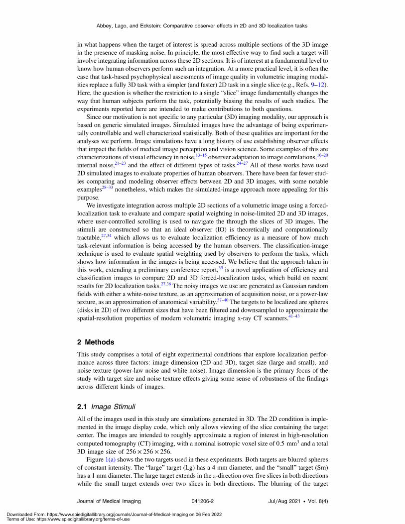
Figure 1(a) shows the two targets used in these experiments. Both targets are blurred spheresof constant intensity. The “large” target (Lg) has a 4 mm diameter, and the “small” target (Sm)has a 1 mm diameter. The large target extends in the z-direction over five slices in both directionswhile the small target extends over two slices in both directions. The blurring of the target

Abbey, Lago, and Eckstein: Comparative observer effects in 2D and 3D localization tasks

Journal of Medical Imaging 041206-2 Jul∕Aug 2021 • Vol. 8(4)

Downloaded From: https://www.spiedigitallibrary.org/journals/Journal-of-Medical-Imaging on 06 Feb 2022Terms of Use: https://www.spiedigitallibrary.org/terms-of-use

profiles is intended to roughly approximate a system transfer function in an imaging context.For simplicity, we use a rotationally symmetric blurring function implemented as a filter in

the FFT domain. For a radial frequency component defined as f ¼ffiffiffiffiffiffiffiffiffiffiffiffiffiffiffiffiffiffiffiffiffiffiffiffiffiffif2x þ f2y þ f2z

q, the transfer

function filter is given by a cosine roll-off function from DC (f ¼ 0) to Nyquist (fNyq ¼1.0 cyc∕mm):

EQ-TARGET;temp:intralink-;e001;116;264TðfÞ ¼�0.5þ 0.5 cosðπf∕fNyqÞ 0 ≤ f ≤ fNyq0 f > fNyq

: (1)

The transfer function falls off from 1 at f ¼ 0 to 0 at fNyq with a full-width at half-max at0.5 cyc∕mm, which is roughly consistent with the transfer properties of high-resolution CTscanners.43 Note that target amplitudes are defined in this work as the amplitude of the disksbefore filtering by the transfer function. This makes them analogous to the amplitude of lesionsin tissue for the medical-imaging context.

Figure 1(b) shows sample slices for the two Gaussian noise textures used as image back-grounds. The two textures consist of white-noise (WN), in which every voxel is an independentGaussian process, and a so-called “power-law” noise (PL) in which the power spectrum of thenoise fields obeys a power-law, 1∕ðf þ εÞ3, with a small offset (ε ¼ 0.0078 cyc∕mm) to avoidinstability near f ¼ 0. The power spectra of both processes are scaled so that the voxel standarddeviation is 20 gray levels, and a mean background of 100 gray levels is used, which keeps in theimages mostly well within the 8-bit display range (256 gray levels) of the monitor. Any voxelsoutside the 8-bit range are truncated to the nearest boundary (0 or 255).

Fig. 1 (a) Targets and noise. The 3D profile of the large target (upper row) and small target(lower row) are shown for �5 slices from the target center. For the 2D task, only the central slice(slice number 0) appears in the image. (b) Examples of the white noise (left) and power-law noise(right) textures used in the experiments. In the 3D tasks, these would be a single slice from avolumetric image.

Abbey, Lago, and Eckstein: Comparative observer effects in 2D and 3D localization tasks

Journal of Medical Imaging 041206-3 Jul∕Aug 2021 • Vol. 8(4)

Downloaded From: https://www.spiedigitallibrary.org/journals/Journal-of-Medical-Imaging on 06 Feb 2022Terms of Use: https://www.spiedigitallibrary.org/terms-of-use

Image backgrounds are generated by initially sampling from a standardized normal randomnumber generator, taking the 3D FFT, multiplying by the square root of the power spectrum,inverse transforming, and then adding the mean background level. A target profile at a specifiedtarget amplitude is then added to the image background at a random location in the central 128 ×128 × 128 region of the volume, and the result is truncated to the 8-bit gray-level range of themonitor. A set of five target amplitudes are mixed across the trials. The procedure for determin-ing these are described in the next section.

2.2 Forced Localization Task

Forced localization is a generalization of the multiple-alternative forced-choice paradigm. Thetarget is always present in the image at an unknown random location, and in each trial the subjectidentifies the location they believe is most likely to be the target center. The response is con-sidered correct if it falls within a distance of 6 pixels (3.6 mm radius on the display) of the actualtarget center.

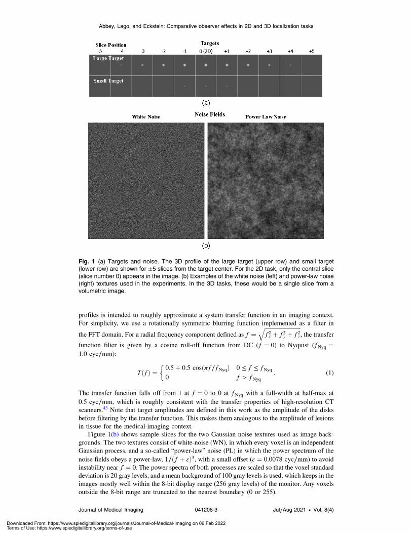
Figure 2 shows the forced-localization interface for the 2D and 3D tasks. For the 2D tasks, asingle slice is shown in the interface, as in Fig. 2(a). This slice is selected to pass through thecenter of the target in the z direction. The observer responds by double-clicking a mouse-drivenpointer on the selected location, which must be in the central 128 × 128 region of the image (i.e.,inside the hash marks at the edge of the image). Responses outside of this area are ignored, and atrial lasts until a valid response is obtained.

In the 3D task shown in Fig. 2(bB), the subjects need to navigate through the volume as partof the localization response. This is accomplished using a mouse click-and-drag, up or downthrough the z range of the 3D image. For fine tuning the slice selection, the up and down arrowson the keyboard can be used to move a single slice at a time. The scroll bar on the right side ofthe 3D interface is used to indicate the position of the current slice in the 3D stack. It also indi-cates the middle 128 slices of the z range (in green). Localization responses are only acceptedwithin this range.

In each experimental condition, the performance is assessed in two phases. In the first “train-ing” phase, an adaptive staircase is used to estimate the 80% correct target amplitude. We use athree-down one-up staircase in which three correct responses result in the next trial having a 15%reduced target amplitude and a single incorrect response leading to a 15% increased target ampli-tude. This staircase is known to oscillate around the 80% correct threshold.44 The staircase startsat high amplitude to give the observer the opportunity to get familiar with the task. It typically

Fig. 2 Localization displays. Display windows for (a) the 2D and (b) 3D stimuli are shown. Theexample images shown are for the large-target in power-law noise condition. A reference image ofthe noiseless target is displayed at the top of the window (in the box), and the trial number is shownin the upper left side of the window. The small hash marks on the edge of the image indicate theX -Y search region. On the 3D display, the scroll-bar on the right side shows the depth of thecurrent slice in the Z direction (blue) along with the depth range (green) of the 3D search region.

Abbey, Lago, and Eckstein: Comparative observer effects in 2D and 3D localization tasks

Journal of Medical Imaging 041206-4 Jul∕Aug 2021 • Vol. 8(4)

Downloaded From: https://www.spiedigitallibrary.org/journals/Journal-of-Medical-Imaging on 06 Feb 2022Terms of Use: https://www.spiedigitallibrary.org/terms-of-use

takes 20 to 30 trials for the first incorrect response to be made. The staircase is run for a totalof 12 reversals, in which the amplitude goes from decreasing to increasing or vice-versa. Thethreshold estimate is derived from the geometric mean of the target amplitude over the last eightreversals. The adaptive staircase procedure is run three times, with the final training thresholdestimate being the average of the three runs.

A total of 500 forced localization trials are used for the test set, which uses five differenttarget amplitudes that are randomly mixed throughout the trials (100 trials at each of the ampli-tudes). This includes the 80% correct threshold estimated from the training runs, as well as�10% of this threshold and �20% of this threshold. The range of amplitudes gives us someability to assess the subjects’ psychometric functions and also ensures that there will be a rea-sonable frequency of difficult cases leading to a sufficient number of incorrect responses forestimating a classification image. In each trial, the display software records the index of thestimulus, the target amplitude of the trial, the true location of the target, the localization responseof the subject, and the reaction time from stimulus display to the recording of a valid mouse click.The true target location is given as x, y, and z indices of the target center. The localizationresponse is coded as x, y, and z indices of the subject-selected image pixel. In the 2D task, thez index of the localization response is constrained to be the target z index. The proportion ofcorrect responses (PC) is used as the measure of performance for a given amplitude. It is com-puted for each of the five amplitudes tested.

The experimental data were collected using a clinical review monitor (Barco Inc.) calibratedto the DICOM standard over a measured luminance range of 0.04 to 165.7 cd∕m2. Images weremagnified by a factor of 2 for a displayed pixel size of 0.6 mm, given the native (isotropic) pixelsize of 0.3 mm. Subjects were encouraged to position themselves at a comfortable viewing dis-tance, which was typically between 50 and 100 cm from the monitor face. For a subject at thecenter of this range, 21.8 pixels subtend a visual angle of 1 deg.

A total of five subjects conducted the studies reported here under an IRB-approved humansubjects protocol at the authors’ institution. The four 2D experiments were completed in roughly30 to 45 min per condition, but the 3D experiments took considerably longer, requiring 3 to 4 hfor each condition. The total time to complete the study for each subject was roughly 20 h, spreadover multiple sessions at the workstation. Four of the subjects were naïve to the purpose of theresearch and compensated for their time, the other subject is the first author.

2.3 Ideal Observer

The Ideal Observer, described in a previous publication,27 was used in the computation of effi-ciency. We briefly review the computations involved in evaluating the IO on a given image here.The first step involves a convolution with the prewhitened matched filter,45 then exponentiationof the result (within the search region) to form a posterior distribution on target location. Asecond scanning operation with a 6-pixel radius disk (in 2D) or sphere (in 3D) is used to computethe posterior utility of each point in the search region. The point that maximizes this utilityfunction over all possible locations is the IO response for the trial.

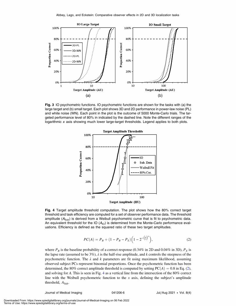
Monte-Carlo studies using many independent sample images at a given target amplitudeare used to assess the performance of the IO in terms of the proportion of correct localizations(PC). Evaluations at a range of target amplitudes can be used to obtain the ideal-observer psy-chometric function, which shows how target amplitude affects performance in each condition.Ideal-observer psychometric functions in all eight experimental conditions are plotted in Fig. 3using 5000 Monte-Carlo trials at each of the target amplitudes. These data are used to get ideal-observer amplitude thresholds for the efficiency computations described next.

2.4 Amplitude Thresholds and Efficiency

Figure 4 shows how subject data and an ideal-observer psychometric function are used to obtainan estimate of human-observer efficiency for a given experimental condition. As describedabove, the psychophysical experiments evaluate five different target amplitudes in each condi-tion from which five performance levels are estimated for each subject. These points are used tofit a Weibull psychometric function,46,47 PCðAÞ, defined as

Abbey, Lago, and Eckstein: Comparative observer effects in 2D and 3D localization tasks

Journal of Medical Imaging 041206-5 Jul∕Aug 2021 • Vol. 8(4)

Downloaded From: https://www.spiedigitallibrary.org/journals/Journal-of-Medical-Imaging on 06 Feb 2022Terms of Use: https://www.spiedigitallibrary.org/terms-of-use

EQ-TARGET;temp:intralink-;e002;116;186PCðAÞ ¼ PB þ ð1 − PB − PEÞ�1 − 2

−�Aλ

�k�; (2)

where PB is the baseline probability of a correct response (0.34% in 2D and 0.04% in 3D), PE isthe lapse rate (assumed to be 3%), λ is the half-rise amplitude, and k controls the steepness of thepsychometric function. The λ and k parameters are fit using maximum likelihood, assumingobserved subject PCs represent binomial proportions. Once the psychometric function has beendetermined, the 80% correct amplitude threshold is computed by setting PCðAÞ ¼ 0.8 in Eq. (2),and solving for A. This is seen in Fig. 4 as a vertical line from the intersection of the 80% correctline with the Weibull psychometric function to the x axis, defining the subject’s amplitudethreshold, ASub.

Fig. 4 Target amplitude threshold computation. The plot shows how the 80% correct targetthreshold and task efficiency are computed for a set of observer performance data. The thresholdamplitude (ASub) is derived from a Weibull psychometric curve that is fit to psychometric data.An equivalent threshold for the IO (AIO) is determined from the Monte-Carlo performance eval-uations. Efficiency is defined as the squared ratio of these two target amplitudes.

Fig. 3 IO psychometric functions. IO psychometric functions are shown for the tasks with (a) thelarge target and (b) small target. Each plot shows 3D and 2D performance in power-law noise (PL)and white noise (WN). Each point in the plot is the outcome of 5000 Monte-Carlo trials. The tar-geted performance level of 80% in indicated by the dashed line. Note the different ranges of thelogarithmic x axis showing much lower large-target thresholds. Legend applies to both plots.

Abbey, Lago, and Eckstein: Comparative observer effects in 2D and 3D localization tasks

Journal of Medical Imaging 041206-6 Jul∕Aug 2021 • Vol. 8(4)

Downloaded From: https://www.spiedigitallibrary.org/journals/Journal-of-Medical-Imaging on 06 Feb 2022Terms of Use: https://www.spiedigitallibrary.org/terms-of-use

The 80% correct amplitude threshold for the IO is computed by a similar process from the IOpsychometric data described above. Since these data are generated from many more trials thanthe human data (5000 trials per datum instead of 100), and a much finer sampling of amplitudes(50 instead of 5), the IO threshold is found by linear interpolation between the nearest two points,yielding AIO. Efficiency with respect to the IO is then defined as the ratio48–50

EQ-TARGET;temp:intralink-;e003;116;675η ¼�AIO

ASub

2

: (3)

2.5 Classification Images

Classification image analysis follows the technique described previously for forced-localizationtasks.27 The classification images are estimated from noise fields of the image stimuli in incorrecttrials.51,52 Within each condition and within each subject, these noise fields are all aligned to the(incorrect) response location and then filtered with the inverse-covariance matrix to disambig-uate the effects of noise correlations. Since the images are generated from a stationary Gaussianprocess, this step is implemented through finite Fourier transforms and the inverse noise powerspectrum. The resulting filtered noise fields are then averaged to obtain the raw classificationimage for each subject in each condition. For the 3D images, this process is implemented usingthe full 3D noise field and 3D inverse-covariance filtering. In the 2D conditions, we use the noisefield of the displayed 2D slice. In this case, inverse-covariance filtering is implemented usingthe slice power-spectrum, which is derived from the 3D power spectrum by integrating in z.The resulting classification images are averaged across subjects for evaluating group effects ofthe experimental conditions.

The raw classification images can be quite noisy themselves, particularly in the power-lawnoise condition where low power-spectral density at higher frequencies can amplify estimationerror. We use two methods to control for noise: smoothing and spatial windowing. The smooth-

ing operation is implemented by filtering in the 2D frequency domain, with f2D ¼ffiffiffiffiffiffiffiffiffiffiffiffiffiffiffif2x þ f2y

q.

For 3D classification images, smoothing is applied to each slice independently. We applysmoothing filters that are unity for f2D < 0.5 cyc∕mm, and roll off for 0.5 ≤ f2D ≤ 1.0 cyc∕mm

with a cosine-bell profile.

2.6 Scanning Models

Classification images are most readily interpreted as representing an estimate of the weights ofa linear template model. This has been demonstrated analytically for detection tasks at a fixedlocation53–55 and empirically for tasks that involve search such as the forced-localization tasksused here.27,56 In localization tasks, the linear template is assumed to scan the entire search regionby a convolution operation, much like the first step of the IO model described above. The locali-zation response of the model is typically generated by taking the maximum response of thetemplate within the search region.

When a classification image is used as the linear kernel of a scanning model, the estimationerror in the classification image can bias performance of the model. Since estimation error isunlikely to be well tuned to a target profile, this bias is typically toward lower performance. Tominimize this effect, we implement a number of steps to control noise in the classificationimages, including frequency filtering, spatial windowing, and radial averaging. These aredescribed in Sec. 4.3.

3 Results

The primary analyses of the experiments are presented here, averaged over subjects. Theseinclude the observed amplitude thresholds and efficiency, response times, and classificationimages in each of the experimental conditions.

Abbey, Lago, and Eckstein: Comparative observer effects in 2D and 3D localization tasks

Journal of Medical Imaging 041206-7 Jul∕Aug 2021 • Vol. 8(4)

Downloaded From: https://www.spiedigitallibrary.org/journals/Journal-of-Medical-Imaging on 06 Feb 2022Terms of Use: https://www.spiedigitallibrary.org/terms-of-use

3.1 Task Performance

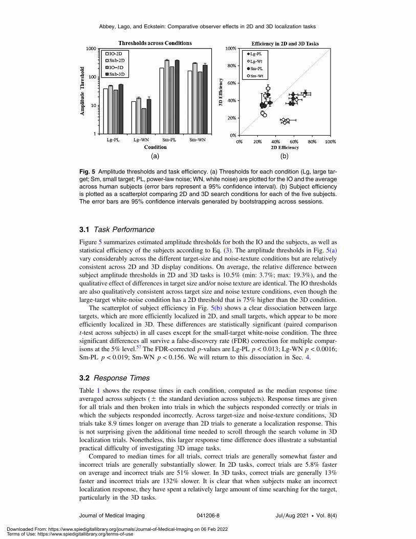
Figure 5 summarizes estimated amplitude thresholds for both the IO and the subjects, as well asstatistical efficiency of the subjects according to Eq. (3). The amplitude thresholds in Fig. 5(a)vary considerably across the different target-size and noise-texture conditions but are relativelyconsistent across 2D and 3D display conditions. On average, the relative difference betweensubject amplitude thresholds in 2D and 3D tasks is 10.5% (min: 3.7%; max: 19.3%), and thequalitative effect of differences in target size and/or noise texture are identical. The IO thresholdsare also qualitatively consistent across target size and noise texture conditions, even though thelarge-target white-noise condition has a 2D threshold that is 75% higher than the 3D condition.

The scatterplot of subject efficiency in Fig. 5(b) shows a clear dissociation between largetargets, which are more efficiently localized in 2D, and small targets, which appear to be moreefficiently localized in 3D. These differences are statistically significant (paired comparisont-test across subjects) in all cases except for the small-target white-noise condition. The threesignificant differences all survive a false-discovery rate (FDR) correction for multiple compar-isons at the 5% level.57 The FDR-corrected p-values are Lg-PL p < 0.013; Lg-WN p < 0.0016;Sm-PL p < 0.019; Sm-WN p < 0.156. We will return to this dissociation in Sec. 4.

3.2 Response Times

Table 1 shows the response times in each condition, computed as the median response timeaveraged across subjects (± the standard deviation across subjects). Response times are givenfor all trials and then broken into trials in which the subjects responded correctly or trials inwhich the subjects responded incorrectly. Across target-size and noise-texture conditions, 3Dtrials take 8.9 times longer on average than 2D trials to generate a localization response. Thisis not surprising given the additional time needed to scroll through the search volume in 3Dlocalization trials. Nonetheless, this larger response time difference does illustrate a substantialpractical difficulty of investigating 3D image tasks.

Compared to median times for all trials, correct trials are generally somewhat faster andincorrect trials are generally substantially slower. In 2D tasks, correct trials are 5.8% fasteron average and incorrect trials are 51% slower. In 3D tasks, correct trials are generally 13%faster and incorrect trials are 132% slower. It is clear that when subjects make an incorrectlocalization response, they have spent a relatively large amount of time searching for the target,particularly in the 3D tasks.

Fig. 5 Amplitude thresholds and task efficiency. (a) Thresholds for each condition (Lg, large tar-get; Sm, small target; PL, power-law noise; WN, white noise) are plotted for the IO and the averageacross human subjects (error bars represent a 95% confidence interval). (b) Subject efficiencyis plotted as a scatterplot comparing 2D and 3D search conditions for each of the five subjects.The error bars are 95% confidence intervals generated by bootstrapping across sessions.

Abbey, Lago, and Eckstein: Comparative observer effects in 2D and 3D localization tasks

Journal of Medical Imaging 041206-8 Jul∕Aug 2021 • Vol. 8(4)

Downloaded From: https://www.spiedigitallibrary.org/journals/Journal-of-Medical-Imaging on 06 Feb 2022Terms of Use: https://www.spiedigitallibrary.org/terms-of-use

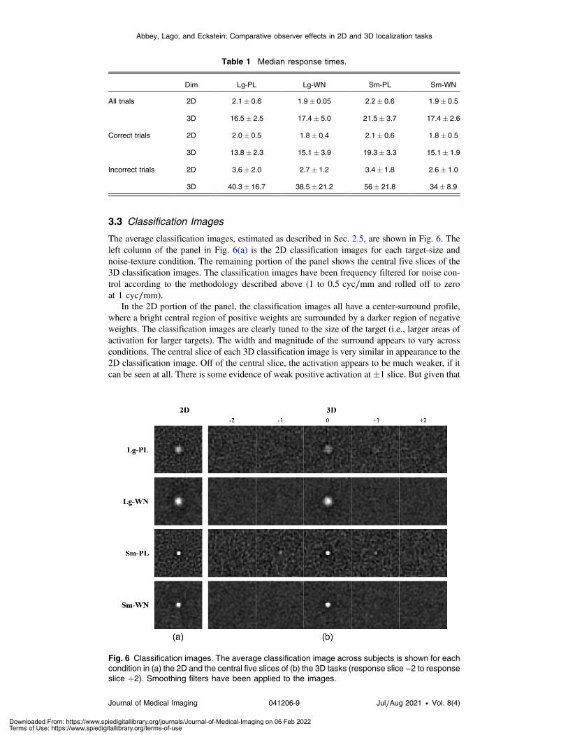
3.3 Classification Images

The average classification images, estimated as described in Sec. 2.5, are shown in Fig. 6. Theleft column of the panel in Fig. 6(a) is the 2D classification images for each target-size andnoise-texture condition. The remaining portion of the panel shows the central five slices of the3D classification images. The classification images have been frequency filtered for noise con-trol according to the methodology described above (1 to 0.5 cyc∕mm and rolled off to zeroat 1 cyc∕mm).

In the 2D portion of the panel, the classification images all have a center-surround profile,where a bright central region of positive weights are surrounded by a darker region of negativeweights. The classification images are clearly tuned to the size of the target (i.e., larger areas ofactivation for larger targets). The width and magnitude of the surround appears to vary acrossconditions. The central slice of each 3D classification image is very similar in appearance to the2D classification image. Off of the central slice, the activation appears to be much weaker, if itcan be seen at all. There is some evidence of weak positive activation at �1 slice. But given that

Fig. 6 Classification images. The average classification image across subjects is shown for eachcondition in (a) the 2D and the central five slices of (b) the 3D tasks (response slice −2 to responseslice þ2). Smoothing filters have been applied to the images.

Table 1 Median response times.

Dim Lg-PL Lg-WN Sm-PL Sm-WN

All trials 2D 2.1� 0.6 1.9� 0.05 2.2� 0.6 1.9� 0.5

3D 16.5� 2.5 17.4� 5.0 21.5� 3.7 17.4� 2.6

Correct trials 2D 2.0� 0.5 1.8� 0.4 2.1� 0.6 1.8� 0.5

3D 13.8� 2.3 15.1� 3.9 19.3� 3.3 15.1� 1.9

Incorrect trials 2D 3.6� 2.0 2.7� 1.2 3.4� 1.8 2.6� 1.0

3D 40.3� 16.7 38.5� 21.2 56� 21.8 34� 8.9

Abbey, Lago, and Eckstein: Comparative observer effects in 2D and 3D localization tasks

Journal of Medical Imaging 041206-9 Jul∕Aug 2021 • Vol. 8(4)

Downloaded From: https://www.spiedigitallibrary.org/journals/Journal-of-Medical-Imaging on 06 Feb 2022Terms of Use: https://www.spiedigitallibrary.org/terms-of-use

the small signal extends over a total of five slices, and the larger target extends over 11 slices,this represents very limited use of multiple slices.

4 Discussion

4.1 Comparisons with Prior Investigations

The results of our studies can be related to findings in some earlier studies. Reiser andNishikawa30 compared 2D and 3D images in a free search task with noise structures that arevery similar to what is used here (white noise and power-law noise) and targets that are closer insize to the large target in this work. They found a pronounced improvement in performance for3D images in the white noise backgrounds, and little—if any—improvement for the power lawnoise. Balta et al.32 also used a power-law background (with additional orientation parameters)with blurred disk targets in a signal-known-exactly task. In this case, a more realistic imageformation model was used that modeled the limited angular range of digital breast tomo-synthesis. They also found similar performance between 2D and 3D images, consistent withReiser and Nishikawa.

We find similar results in Fig. 5(a) for the ideal- and human-observer amplitude thresholddata, although our difference is somewhat less dramatic than the finding in Reiser andNishikawa. In white noise, the large-target amplitude thresholds drop in 3D relative to 2D,whereas in power-law noise they stay approximately the same. Thus, the absolute performanceeffects appear to have some robustness properties. However, Fig. 5(b) shows the importanceof considering task efficiency as well. While observer performance localizing the large targetis roughly equivalent in 3D and 2D images (the 3D amplitude threshold is 7% larger for power-law noise and 11% smaller for white noise), the subjects are considerably more efficient in the2D task than the 3D task (44% more efficient in power-law noise and 108% more efficient forwhite noise).

4.2 Dissociation between Large and Small Target Efficiency

If we consider these tasks from the perspective of the threshold amplitude, shown in Fig. 5(a),then it is clear that the small targets are substantially more difficult to localize accurately than thelarge targets in both 2D and 3D tasks with thresholds that are 7 to 17 times larger. There are twopossible reasons for this large discrepancy: (1) the tasks with small targets are inherently moredifficult or (2) human observers are less effective at localizing the small targets. The efficiencyvalues in Fig. 5(b) help disambiguate these two effects by correcting for task difficulty and there-fore isolating reader performance effects. In this context, the reader results show a dissociation inwhich large targets are more efficiently localized in the 2D tasks and the small targets are moreefficiently localized in the 3D tasks.

This finding would appear to be at odds with recent studies by Lago, Eckstein, and col-leagues,33,58–60 demonstrating substantial performance reductions for small targets in 3D searchtasks. However, it is important to note a fundamental difference between those experiments andthe results reported here. Their investigations examine the role of peripheral vision in modulatingsearch performance in 2D and 3D images. Their images can occupy a much larger portion of thevisual field than these studies (up to 30-deg visual angle). The search region used in these experi-ments can be mostly or entirely covered by central vision. Clinical ophthalmology texts definethe fovea (including the perifovea) as occupying the central 8 deg of the visual field.61 With thisdefinition and our display procedure described, the entire 128 × 128 search region fits in thefovea at a viewing distance of 76 cm or more. At a close viewing distance of 50 cm, 67% ofthe search region is covered by the fovea. Given the search region size and subject viewingdistance, it is perhaps not surprising that we do not see evidence of peripheral vision effects.

The classification images, on the other hand, suggest that a major source of inefficiency forlarge targets is the lack of spatial integration across multiple slices in the 3D images, whenviewed by scrolling. The spatial weights in the classification images are largely gone after thecentral slice. This can be seen in the off-center slices of the 3D classification images in Fig. 6.

Abbey, Lago, and Eckstein: Comparative observer effects in 2D and 3D localization tasks

Journal of Medical Imaging 041206-10 Jul∕Aug 2021 • Vol. 8(4)

Downloaded From: https://www.spiedigitallibrary.org/journals/Journal-of-Medical-Imaging on 06 Feb 2022Terms of Use: https://www.spiedigitallibrary.org/terms-of-use

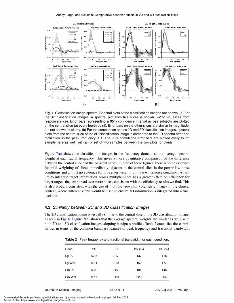
Figure 7(a) shows the classification images in the frequency domain as the average spectralweight at each radial frequency. This gives a more quantitative comparison of the differencebetween the central slice and the adjacent slices. In both of these figures, there is some evidencefor mild weighting of slices immediately adjacent to the central slice in the power-law noiseconditions and almost no evidence for off-center weighting in the white noise condition. A fail-ure to integrate target information across multiple slices has a greater effect on efficiency forlarger targets that are spread over more slices, consistent with the efficiency results we find. Thisis also broadly consistent with the use of multiple views for volumetric images in the clinicalcontext, where different views would be used to ensure 3D information is integrated into a finaldecision.

4.3 Similarity between 2D and 3D Classification Images

The 2D classification image is visually similar to the central slice of the 3D classification image,as seen in Fig. 6. Figure 7(b) shows that the average spectral weights are similar as well, withboth 2D and 3D classification images adopting bandpass profiles. Table 2 quantifies these simi-larities in terms of the common bandpass features of peak frequency and fractional bandwidth

Fig. 7 Classification-image spectra. Spectral plots of the classification images are shown. (a) Forthe 3D classification images, a spectral plot from five slices is shown (−2 to þ2 slices fromresponse slice). Error bars representing a 95% confidence interval across subjects are plottedon the central slice (at every fourth point). Error bars on the other slices are similar in magnitude,but not shown for clarity. (b) For the comparison across 2D and 3D classification images, spectralplots from the central slice of the 3D classification image is compared to the 2D spectra after nor-malization so the peak frequency is 1. The 95% confidence error bars are plotted every fourthsample here as well, with an offset of two samples between the two plots for clarity.

Table 2 Peak frequency and fractional bandwidth for each condition.

Cond 2D 3D 2D (%) 3D (%)

Lg-PL 0.15 0.17 137 118

Lg-WN 0.11 0.10 150 177

Sm-PL 0.28 0.27 181 146

Sm-WN 0.17 0.20 223 204

Abbey, Lago, and Eckstein: Comparative observer effects in 2D and 3D localization tasks

Journal of Medical Imaging 041206-11 Jul∕Aug 2021 • Vol. 8(4)

Downloaded From: https://www.spiedigitallibrary.org/journals/Journal-of-Medical-Imaging on 06 Feb 2022Terms of Use: https://www.spiedigitallibrary.org/terms-of-use

(FWHM relative to peak frequency). The average relative difference between 2D and 3D con-ditions is −4% for peak frequency and 8% for fractional bandwidth. For comparison, considerthe average relative difference between power-law and white noise, which is −34% for peakfrequency and 31% for fractional bandwidth. Alternatively, the average relative differencebetween the large target and the small targets is 75% for peak frequency and 30% for fractionalbandwidth. Thus, relative to other effects in these data, differences between 2D and the centralslice of the 3D classification images are small.

This similarity between 2D and 3D classification images, along with the lack of substantiveoff-center weighting in the 3D classification images, establishes a mechanistic similarity be-tween the 2D and 3D localization tasks. Despite the differences in image display and regardlessof the search procedure used, subjects appear to be localizing targets in the 3D images as if theywere looking mainly at that 2D slice. This lends some credence to the practice of evaluating 3Dimages using a single 2D slice, although there are many potential caveats and limitations to thisstatement as described below.

4.4 Classification Images as Kernels of a Scanning Localization Model

The classification image can be interpreted as an estimate of the filter kernel27,36 in the context ofscanning models of localization performance. In fact, validation of classification-image estima-tion for localization tasks is based on generating responses from a scanning linear model andshowing that the classification image accurately estimates the kernel of this model. This class ofmodel has been used to understand search in medical images previously,62–65 although the recentresults of Lago et al.59,60 serve as a caution when peripheral vision effects may be present.Nonetheless, the classification images can be used to understand how much of the subject’sefficiency is due to the spatial weighting implemented in the scanning kernel and how muchis due to other processes in the localization tasks (e.g., inefficient search or internal noise).

Estimation error is an important issue for implementing the classification images in scan-ning models. Noise in the classification image estimate will tend to reduce performance (andtherefore the localization efficiency) of the model since it is unlikely that estimation error willbe well tuned to a target profile. To mitigate the effects of estimation error, we use relativelyaggressive filtering of the classification images based on the frequency profiles shown in Fig. 7.For the large targets, the smoothing filter extends to 0.3 cyc∕mm before rolling off to zero witha cosine profile at 0.6 cyc∕mm. For the small targets (which extend further into the frequencydomain), the smoothing filter is constant to a frequency of 0.6 cyc∕mm and rolls off to zero at1 cyc∕mm (which is identical to the filtering used in Fig. 6). In addition, radial averaging isused to smooth radial bands in the spatial domain, under the assumption of approximate rota-tional symmetry, and a spatial window is applied under the assumption of a relatively compactfilter kernel. This spatial window is also tuned to the size of the targets. For the large targets, thespatial window is constant out to a radius of 4 mm and rolls off to zero at 6 mm with a cosineprofile. For the small targets, the spatial window is constant out to a radius of 2 mm and rolls offto zero at 4 mm.

Figure 8(a) shows an example of the effects of different filtering procedures on the classi-fication image. A raw classification image for a given subject in one of the tasks (PL-Sm) isshown along with the “display processed” version that has been frequency-filtered as in Fig. 6,and a “kernel processed” version that has been processed as described above. The kernel proc-essed image is seen to be largely devoid of visible estimation error. For the 3D classificationimages, kernel processing is applied to the central three slices, with slices outside this range set tozero. Figure 8(b) shows the real component of the frequency spectrum for the various versions ofthe classification image. The display processed classification image is seen to have frequenciesmodulated starting at 0.5 cyc∕mm and completely eliminated at 1 cyc∕mm, consistent with thefilter used to smooth the image data. The spectrum of the kernel-processed classification image isseen to have a spectrum that is generally consistent with the others, but substantially smoother.

Figure 9 shows the average subject efficiency as a function of the average efficiency of theclassification-image-derived scanning models. In previous work,36 task efficiency has been rea-sonably well modeled as kernel efficiency minus 12.6% points with a coefficient of determi-nation (R2) of 0.86. While that relationship seems to hold reasonably well on average in

Abbey, Lago, and Eckstein: Comparative observer effects in 2D and 3D localization tasks

Journal of Medical Imaging 041206-12 Jul∕Aug 2021 • Vol. 8(4)

Downloaded From: https://www.spiedigitallibrary.org/journals/Journal-of-Medical-Imaging on 06 Feb 2022Terms of Use: https://www.spiedigitallibrary.org/terms-of-use

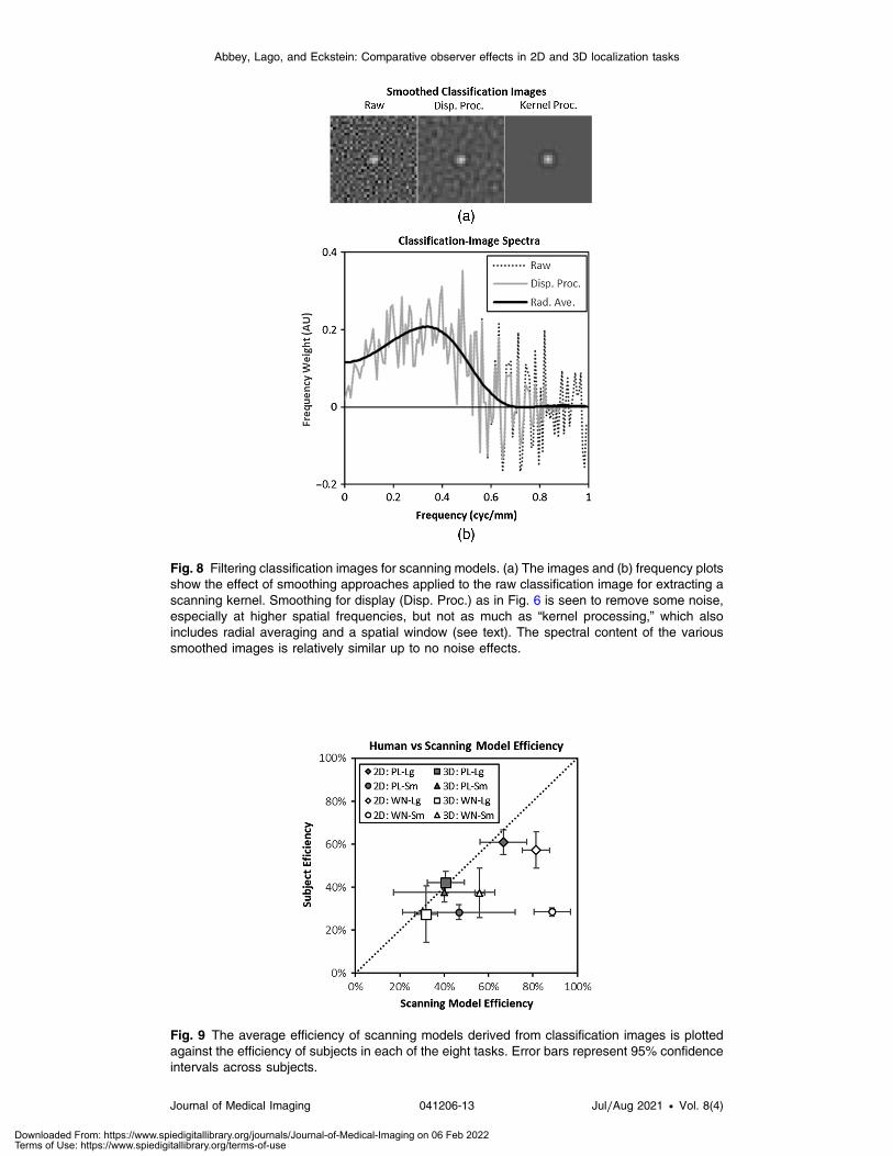
Fig. 8 Filtering classification images for scanning models. (a) The images and (b) frequency plotsshow the effect of smoothing approaches applied to the raw classification image for extracting ascanning kernel. Smoothing for display (Disp. Proc.) as in Fig. 6 is seen to remove some noise,especially at higher spatial frequencies, but not as much as “kernel processing,” which alsoincludes radial averaging and a spatial window (see text). The spectral content of the varioussmoothed images is relatively similar up to no noise effects.

Fig. 9 The average efficiency of scanning models derived from classification images is plottedagainst the efficiency of subjects in each of the eight tasks. Error bars represent 95% confidenceintervals across subjects.

Abbey, Lago, and Eckstein: Comparative observer effects in 2D and 3D localization tasks

Journal of Medical Imaging 041206-13 Jul∕Aug 2021 • Vol. 8(4)

Downloaded From: https://www.spiedigitallibrary.org/journals/Journal-of-Medical-Imaging on 06 Feb 2022Terms of Use: https://www.spiedigitallibrary.org/terms-of-use

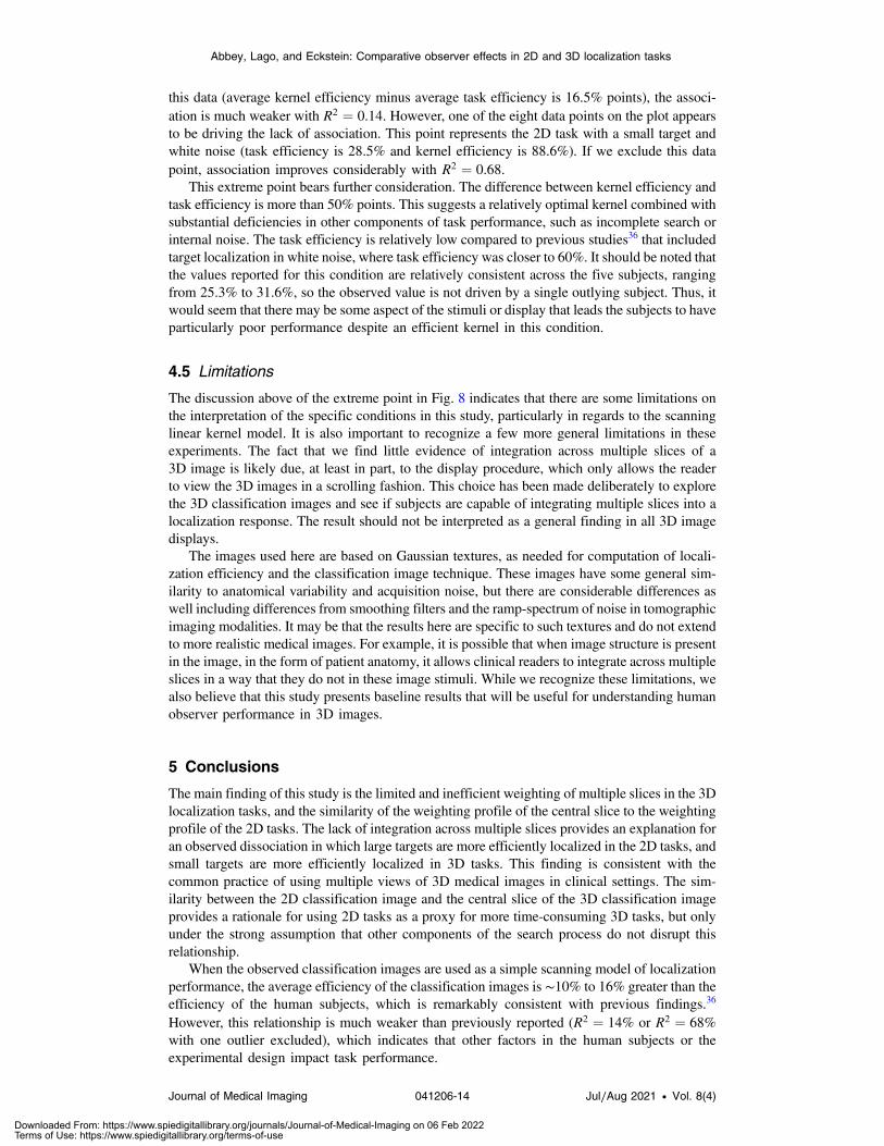
this data (average kernel efficiency minus average task efficiency is 16.5% points), the associ-ation is much weaker with R2 ¼ 0.14. However, one of the eight data points on the plot appearsto be driving the lack of association. This point represents the 2D task with a small target andwhite noise (task efficiency is 28.5% and kernel efficiency is 88.6%). If we exclude this datapoint, association improves considerably with R2 ¼ 0.68.

This extreme point bears further consideration. The difference between kernel efficiency andtask efficiency is more than 50% points. This suggests a relatively optimal kernel combined withsubstantial deficiencies in other components of task performance, such as incomplete search orinternal noise. The task efficiency is relatively low compared to previous studies36 that includedtarget localization in white noise, where task efficiency was closer to 60%. It should be noted thatthe values reported for this condition are relatively consistent across the five subjects, rangingfrom 25.3% to 31.6%, so the observed value is not driven by a single outlying subject. Thus, itwould seem that there may be some aspect of the stimuli or display that leads the subjects to haveparticularly poor performance despite an efficient kernel in this condition.

4.5 Limitations

The discussion above of the extreme point in Fig. 8 indicates that there are some limitations onthe interpretation of the specific conditions in this study, particularly in regards to the scanninglinear kernel model. It is also important to recognize a few more general limitations in theseexperiments. The fact that we find little evidence of integration across multiple slices of a3D image is likely due, at least in part, to the display procedure, which only allows the readerto view the 3D images in a scrolling fashion. This choice has been made deliberately to explorethe 3D classification images and see if subjects are capable of integrating multiple slices into alocalization response. The result should not be interpreted as a general finding in all 3D imagedisplays.

The images used here are based on Gaussian textures, as needed for computation of locali-zation efficiency and the classification image technique. These images have some general sim-ilarity to anatomical variability and acquisition noise, but there are considerable differences aswell including differences from smoothing filters and the ramp-spectrum of noise in tomographicimaging modalities. It may be that the results here are specific to such textures and do not extendto more realistic medical images. For example, it is possible that when image structure is presentin the image, in the form of patient anatomy, it allows clinical readers to integrate across multipleslices in a way that they do not in these image stimuli. While we recognize these limitations, wealso believe that this study presents baseline results that will be useful for understanding humanobserver performance in 3D images.

5 Conclusions

The main finding of this study is the limited and inefficient weighting of multiple slices in the 3Dlocalization tasks, and the similarity of the weighting profile of the central slice to the weightingprofile of the 2D tasks. The lack of integration across multiple slices provides an explanation foran observed dissociation in which large targets are more efficiently localized in the 2D tasks, andsmall targets are more efficiently localized in 3D tasks. This finding is consistent with thecommon practice of using multiple views of 3D medical images in clinical settings. The sim-ilarity between the 2D classification image and the central slice of the 3D classification imageprovides a rationale for using 2D tasks as a proxy for more time-consuming 3D tasks, but onlyunder the strong assumption that other components of the search process do not disrupt thisrelationship.

When the observed classification images are used as a simple scanning model of localizationperformance, the average efficiency of the classification images is ∼10% to 16% greater than theefficiency of the human subjects, which is remarkably consistent with previous findings.36

However, this relationship is much weaker than previously reported (R2 ¼ 14% or R2 ¼ 68%

with one outlier excluded), which indicates that other factors in the human subjects or theexperimental design impact task performance.

Abbey, Lago, and Eckstein: Comparative observer effects in 2D and 3D localization tasks

Journal of Medical Imaging 041206-14 Jul∕Aug 2021 • Vol. 8(4)

Downloaded From: https://www.spiedigitallibrary.org/journals/Journal-of-Medical-Imaging on 06 Feb 2022Terms of Use: https://www.spiedigitallibrary.org/terms-of-use

Disclosures

The authors have no conflicts of interest to declare.

Acknowledgments

This work was supported by funding from the National Institutes of Health (NIH) (R01-EB026427 and R01-EB025829) and was based partly on scientific content previously reportedin the SPIE Medical Imaging meeting.35

References

1. H. H. Barrett and K. J. Myers, Foundations of Image Science, Wiley Series in Pure andApplied Optics, pp. xli, 1540, Wiley-Interscience, Hoboken, New Jersey (2004).

2. J. T. Bushberg et al., The Essential Physics of Medical Imaging, 4th ed., Wolters Kluwer,Philaelphia, Pennsylvania (2021).

3. D. Maupu et al., “3D stereo interactive medical visualization,” IEEE Comput. GraphicsAppl. 25(5), 67–71 (2005).

4. D. J. Getty and P. J. Green, “Clinical applications for stereoscopic 3D displays,” J. Soc. Inf.Disp. 15(6), 377–384 (2007).

5. Z. Lu and Y. Sakamoto, “Holographic display methods for volume data: polygon-basedand MIP-based methods,” Appl. Opt. 57(1), A142–A149 (2018).

6. P. S. Calhoun et al., “Three-dimensional volume rendering of spiral CT data: theory andmethod,” Radiographics 19(3), 745–764 (1999).

7. M. Smelyanskiy et al., “Mapping high-fidelity volume rendering for medical imaging toCPU, GPU and many-core architectures,” IEEE Trans. Visualization Comput. Graphics15(6), 1563–1570 (2009).

8. G. D. Rubin et al., “Perspective volume rendering of CT and MR images: applications forendoscopic imaging,” Radiology 199(2), 321–330 (1996).

9. D. J. Kadrmas et al., “Impact of time-of-flight on PET tumor detection,” J. Nucl. Med. 50(8),1315–1323 (2009).

10. N. J. Packard et al., “Effect of slice thickness on detectability in breast CT using a pre-whitened matched filter and simulated mass lesions,” Med. Phys. 39(4), 1818–1830(2012).

11. H. W. Tseng et al., “Assessing image quality and dose reduction of a new x-ray computedtomography iterative reconstruction algorithm using model observers,” Med. Phys. 41(7),071910 (2014).

12. D. Racine et al., “Task-based quantification of image quality using a model observer inabdominal CT: a multicentre study,” Eur. Radiol. 28(12), 5203–5210 (2018).

13. A. E. Burgess et al., “Efficiency of human visual signal discrimination,” Science 214(4516),93–94 (1981).

14. A. Burgess and H. Ghandeharian, “Visual signal detection. I. Ability to use phase informa-tion,” J. Opt. Soc. Am. A 1(8), 900–5 (1984).

15. A. E. Burgess and H. Ghandeharian, “Visual signal detection. II. Signal-location identifi-cation,” J. Opt. Soc. Am. A 1(8), 906–910 (1984).

16. K. J. Myers et al., “Effect of noise correlation on detectability of disk signals in medicalimaging,” J. Opt. Soc. Am. A 2(10), 1752–1759 (1985).

17. K. J. Myers and H. H. Barrett, “Addition of a channel mechanism to the ideal-observermodel,” J. Opt. Soc. Am. A 4(12), 2447–2457 (1987).

18. J. P. Rolland and H. H. Barrett, “Effect of random background inhomogeneity on observerdetection performance,” J. Opt. Soc. Am. A 9(5), 649–658 (1992).

19. A. E. Burgess, X. Li, and C. K. Abbey, “Visual signal detectability with two noisecomponents: anomalous masking effects,” J. Opt. Soc. Am. A 14(9), 2420–2442 (1997).

20. C. K. Abbey and M. P. Eckstein, “Classification images for simple detection and discrimi-nation tasks in correlated noise,” J. Opt. Soc. Am. A 24(12), B110–B124 (2007).

Abbey, Lago, and Eckstein: Comparative observer effects in 2D and 3D localization tasks

Journal of Medical Imaging 041206-15 Jul∕Aug 2021 • Vol. 8(4)

Downloaded From: https://www.spiedigitallibrary.org/journals/Journal-of-Medical-Imaging on 06 Feb 2022Terms of Use: https://www.spiedigitallibrary.org/terms-of-use

21. A. J. Ahumada, “Putting the visual system noise back in the picture,” J. Opt. Soc. Am. A4(12), 2372–2378 (1987).

22. A. Burgess and B. Colborne, “Visual signal detection. IV. Observer inconsistency,” J. Opt.Soc. Am. A 5(4), 617–627 (1988).

23. Z.-L. Lu and B. A. Dosher, “Characterizing human perceptual inefficiencies with equivalentinternal noise,” J. Opt. Soc. Am. A 16(3), 764–778 (1999).

24. A. Ahumada and A. Watson, “Equivalent-noise model for contrast detection and discrimi-nation,” J. Opt. Soc. Am. A 2(7), 1133–1139 (1985).

25. G. E. Legge, D. Kersten, and A. E. Burgess, “Contrast discrimination in noise,” J. Opt. Soc.Am. A 4(2), 391–404 (1987).

26. C. K. Abbey and M. P. Eckstein, “Classification images for detection, contrast discri-mination, and identification tasks with a common ideal observer,” J. Vision 6(4), 4–55(2006).

27. C. K. Abbey and M. P. Eckstein, “Observer efficiency in free-localization tasks with corre-lated noise,” Front. Psychol. 5, 1–13 (2014).

28. C. Lartizien, P. E. Kinahan, and C. Comtat, “A lesion detection observer study comparing2-dimensional versus fully 3-dimensional whole-body PET imaging protocols,” J. Nucl.Med. 45(4), 714–723 (2004).

29. J.-S. Kim et al., “A comparison of planar versus volumetric numerical observers for detec-tion task performance in whole-body PET imaging,” IEEE Trans. Nucl. Sci. 51(1), 34–40(2004).

30. I. Reiser and R. M. Nishikawa, “Human observer performance in a single slice or a volume:effect of background correlation,” Lect. Notes Comput. Sci. 6136, 327–333 (2010).

31. L. Platisa et al., “Channelized Hotelling observers for the assessment of volumetric imagingdata sets,” J. Opt. Soc. Am. A 28(6), 1145–1163 (2011).

32. C. Balta et al., “2D single-slice vs. 3D viewing of simulated tomosynthesis images of asmall-scale breast tissue model,” Proc. SPIE 10952, 109520V (2019).

33. M. A. Lago et al., “Under-exploration of three-dimensional images leads to search errors forsmall salient targets,” Curr. Biol. 31 In Press (2021).

34. P. Khurd and G. Gindi, “Decision strategies that maximize the area under the LROC curve,”IEEE Trans. Med. Imaging 24(12), 1626–1636 (2005).

35. C. K. Abbey, M. A. Lago, and M. P. Eckstein, “Observer templates in 2D and 3D locali-zation tasks,” Proc. SPIE 10577, 105770T (2018).

36. C. K. Abbey et al., “Classification images for localization performance in ramp-spectrumnoise,” Med. Phys. 45(5), 1970–1984 (2018).

37. A. E. Burgess, F. L. Jacobson, and P. F. Judy, “Human observer detection experiments withmammograms and power-law noise,” Med. Phys. 28(4), 419–437 (2001).

38. K. G. Metheany et al., “Characterizing anatomical variability in breast CT images,” Med.Phys. 35(10), 4685–4694 (2008).

39. L. Chen et al., “Anatomical complexity in breast parenchyma and its implications for opti-mal breast imaging strategies,” Med. Phys. 39(3), 1435–1441 (2012).

40. E. Engstrom, I. Reiser, and R. Nishikawa, “Comparison of power spectra for tomosynthesisprojections and reconstructed images,” Med. Phys. 36(5), 1753–1758 (2009).

41. H. Onishi et al., “Phantom study of in-stent restenosis at high-spatial-resolution CT,”Radiology 289(1), 255–260 (2018).

42. L. J. Oostveen et al., “Physical evaluation of an ultra-high-resolution CT scanner,” Eur.Radiol. 30, 2552–2560 (2020).

43. A. M. Hernandez et al., “Validation of synthesized normal-resolution image data generatedfrom high-resolution acquisitions on a commercial CT scanner,” Med. Phys. 47(10),4775–4785 (2020).

44. M. A. García-Pérez, “Forced-choice staircases with fixed step sizes: asymptotic and small-sample properties,” Vision Res. 38(12), 1861–1881 (1998).

45. R. F. Wagner and G. G. Brown, “Unified SNR analysis of medical imaging systems,” Phys.Med. Biol. 30(6), 489–518 (1985).

46. A. B. Watson and D. G. Pelli, “QUEST: a Bayesian adaptive psychometric method,”Percept. Psychophys. 33(2), 113–120 (1983).

Abbey, Lago, and Eckstein: Comparative observer effects in 2D and 3D localization tasks

Journal of Medical Imaging 041206-16 Jul∕Aug 2021 • Vol. 8(4)

Downloaded From: https://www.spiedigitallibrary.org/journals/Journal-of-Medical-Imaging on 06 Feb 2022Terms of Use: https://www.spiedigitallibrary.org/terms-of-use

47. S. A. Klein, “Measuring, estimating, and understanding the psychometric function: acommentary,” Percept. Psychophys. 63(8), 1421–1455 (2001).

48. D. G. Pelli, “Uncertainty explains many aspects of visual contrast detection and discrimi-nation,” J. Opt. Soc. Am. A 2(9), 1508–1532 (1985).

49. D. Kersten, “Statistical efficiency for the detection of visual noise,” Vision Res. 27(6),1029–1040 (1987).

50. D. Kersten, “Spatial summation in visual noise,” Vision Res. 24(12), 1977–1990 (1984).51. A. J. Ahumada and J. Lovell, “Stimulus features in signal detection,” J. Acoust. Soc. Am.

49(6B), 1751–1756 (1971).52. R. F. Murray, “Classification images: a review,” J. Vision 11(5), 2 (2011).53. C. K. Abbey and M. P. Eckstein, “Classification image analysis: estimation and statistical

inference for two-alternative forced-choice experiments,” J. Vision 2(1), 5 (2002).54. R. F. Murray, P. J. Bennett, and A. B. Sekuler, “Optimal methods for calculating classifi-

cation images: weighted sums,” J. Vision 2(1), 6 (2002).55. C. K. Abbey and M. P. Eckstein, “Optimal shifted estimates of human-observer templates

in two-alternative forced-choice experiments,” IEEE Trans. Med. Imaging 21(5), 429–440(2002).

56. C. K. Abbey et al., “Approximate maximum likelihood estimation of scanning observertemplates,” Proc. SPIE 9416, 94160O (2015).

57. Y. Benjamini and Y. Hochberg, “Controlling the false discovery rate: a practical and power-ful approach to multiple testing,” J. R. Stat. Soc. Ser. B 57(1), 289–300 (1995).

58. M. P. Eckstein, M. A. Lago, and C. K. Abbey, “The role of extra-foveal processing in 3Dimaging,” Proc. SPIE 10136, 101360E (2017).

59. M. A. Lago et al., “Interactions of lesion detectability and size across single-slice DBT and3D DBT,” Proc. SPIE 10577, 105770X (2018).

60. M. A. Lago et al., “Measurement of the useful field of view for single slices of differentimaging modalities and targets,” J. Med. Imaging 7(2), 022411 (2020).

61. L. A. Remington, Clinical Anatomy and Physiology of the Visual System, 3rd ed., ElsevierHealth Sciences, St. Louis, Missouri (2011).

62. R. G. Swensson and P. F. Judy, “Detection of noisy visual targets: models for the effects ofspatial uncertainty and signal-to-noise ratio,” Percept. Psychophys. 29(6), 521–534 (1981).

63. R. G. Swensson, “Unified measurement of observer performance in detecting and localizingtarget objects on images,” Med. Phys. 23(10), 1709–1725 (1996).

64. H. C. Gifford et al., “A comparison of human and model observers in multislice LROCstudies,” IEEE Trans. Med. Imaging 24(2), 160–169 (2005).

65. H. C. Gifford, Z. Liang, and M. Das, “Visual-search observers for assessing tomographicx-ray image quality,” Med. Phys. 43(3), 1563–1575 (2016).

Craig K. Abbey is a researcher in the Department of Psychological & Brain Sciences at UCSanta Barbara. His training is in the field of applied mathematics, and his research focuseson assessment of medical imaging devices and image processing in terms of performance indiagnostic and quantitative tasks.

Miguel A. Lago was a postdoctoral scholar in the Department of Psychological and BrainSciences at the University of California Santa Barbara. He has recently moved to the Food andDrug Administration as a visiting scientist. His background is in computer engineering and hisresearch studies how visual search in 3D medical image modalities affect observer performanceand efficiency in radiology.

Miguel P. Eckstein is a professor in the Department of Psychological and Brain Sciences andaffiliate faculty in the Department of Electrical and Computer Engineering at the Universityof California Santa Barbara. His research uses a variety of tools including behavioral psycho-physics, eye tracking, electro-encephalography, functional magnetic resonance imaging, andcomputational modeling to study how humans see. His findings are applied to problems in medi-cal imaging, computer vision, and interactions between robots/computer systems and humans.

Abbey, Lago, and Eckstein: Comparative observer effects in 2D and 3D localization tasks

Journal of Medical Imaging 041206-17 Jul∕Aug 2021 • Vol. 8(4)

Downloaded From: https://www.spiedigitallibrary.org/journals/Journal-of-Medical-Imaging on 06 Feb 2022Terms of Use: https://www.spiedigitallibrary.org/terms-of-use